Computing the CEV option pricing formula using
the semiclassical approximation of path integral

Abstract

The Constant Elasticity of Variance (CEV) model significantly outperforms the Black-Scholes (BS) model in forecasting both prices and options. Furthermore, the CEV model has a marked advantage in capturing basic empirical regularities such as: heteroscedasticity, the leverage effect, and the volatility smile. In fact, the performance of the CEV model is comparable to most stochastic volatility models, but it is considerable easier to implement and calibrate. Nevertheless, the standard CEV model solution, using the non-central chi-square approach, still presents high computational times, specially when: i) the maturity is small, ii) the volatility is low, or iii) the elasticity of the variance tends to zero. In this paper, a new numerical method for computing the CEV model is developed. This new approach is based on the semiclassical approximation of Feynman’s path integral. Our simulations show that the method is efficient and accurate compared to the standard CEV solution considering the pricing of European call options.

Keywords: Option pricing, constant elasticity of variance model, path integral, numerical methods.

1 Introduction

One of the most significant limitations of the Black-Scholes (BS) [1] model is the assumption of constant volatility, which ignores some well-known empirical regularities such as: the leverage effect [2, 3], and the volatility smile [4, 5]. These shortcomings have inspired several non-constant volatility models in continuous time, considering ‘stochastic volatility’ or ‘level-dependent volatility’ models [10]. In the former, both the asset and the volatility have their own diffusion processes. In the level-dependent volatility models only the asset is governed by a diffusion process, and its volatility is modeled in function of the asset level. In this paper, the analysis will be focused on the the constant elasticity of variance (CEV) model, proposed by J. Cox, the most known level-dependent volatility approach [11, 12].

Furthermore, the CEV model has a marked advantage in capturing basic empirical regularities such as: heteroscedasticity, the leverage effect, and the volatility smile[13, 14, 15, 16]. As a consequence, the CEV model significantly outperforms the Black-Scholes (BS) model in forecasting both prices and options [17, 18, 19, 20, 21]. Furthermore, the performance of the CEV model is comparable to most stochastic volatility models, but it is considerable easier to implement and calibrate [22].

In terms of the option pricing using the CEV model, the exact formula for a vanilla European option involves a complex computation of an infinite series of incomplete gamma functions [11]. Subsequently, [14] matched the Cox pricing formula with the non-central chi-square distribution. Schroder also provides a simple approximated method for its computation, see [23] for a detailed derivation of the two methodologies. Since then, the use of the non-central chi-square distribution becomes the most widely used method of pricing for options under the CEV model. Besides, several alternative methods for its implementation have been developed [24].

Nevertheless, the standard CEV model solutions, using the non-central chi-square approach, still presents considerably high computational times, specially when: i) the maturity is small, ii) the volatility is low, or iii) the elasticity of the variance tends to zero[14, 25, 26]. In order to deal with these problems, many approaches have been reported for the European-vanilla type option pricing. These approaches include numerical schemes [27, 25, 28, 29], Montecarlo simulations [30], perturbation theory model [31], and analytical approximations to the transition density [32] or to the hedging strategy [33], among others.

In this paper, a new numerical method for computing the CEV model is developed. This new approach is based on the semiclassical approximation of Feynman’s path integral model. In financial literature, path integral techniques have already been used in the option pricing problem, see [34, 35, 36, 37, 38, 39]. Nevertheless, the main focus has been in theoretical issues rather than in practical applications. On the other hand, the application of the semiclassical approximation of Feynman’s path integral technique on financial problems is rather limited, see for example [40, 41, 42].

[42] points out that, just as in the case of quantum mechanics, the path integral approach in finance is neither a panacea, nor is it intended to yield fundamentally new results, but in some cases it provides clarity and insight into old problems. In this paper, we analyze the possibility that the path integral approach could also be an interesting computational tool to solve complex problems in quantitative finance. In this context, this research could be important not only because it develops a novel and efficient technique for the solution of the renowned CEV model, but also because it could open the door to computational applications of such methods of quantum mechanics. Indeed, our simulations show that computing the CEV option pricing formula using the semiclassical approximation of path integral is efficient and accurate compared to the standard CEV solution considering the pricing of European call options. Additionally, the proposed approximation reduces execution times importantly and keep the simplicity of the traditional solution.

Thus, the main idea of the paper is twofold, firstly to use ideas from quantum mechanics to deal with applied finance problems, and secondly, to develop practical methodologies and to test them numerically in specific case studies, while discussing their practical advantage and limitations. The structure of the paper is the following. Firstly, Feynman’s path integral formulation is revisited. Secondly, the path integral approximation is applied to the basic BS model. Thirdly, the path integral approximation is applied to the CEV model. Later, a numerical solution to the CEV model is developed. In the next section, several numerical simulations are carried out in order to measure the performance of the new method, comparing the path integral approximation with the traditional non-central chi-squared approach for the pricing of European call options. Finally, some conclusions and future research avenues are outlined.

2 The Feynman path integral approach

The path integral formalism was developed by Richard P. Feynman [43], introducing the action principle from classical mechanics to quantum mechanics. Nowadays Feynman’s path integral is a well-known tool in quantum mechanics, and statistical and mathematical physics, with applications in many branches of physics such as: optics, thermodynamics, nuclear physics, atomic and molecular physics, cosmology, polymer science and other interdisciplinary areas [44, 45].

In the following lines, we describe the fundamentals of the path integral methodology. The starting point is the Schrödinger equation:

$$i\hbar\frac{\partial\Psi}{\partial\tilde{t}}=\mathrm{\hat{H}}_{BS}\Psi$$ (1)

where $\Psi$ is the wave function and $\hat{\mathrm{H}}$ the Hamiltonian quantum operator (for this instance we consider a time independent Hamiltonian).

Considering $\Psi_{0}(x)$ as the initial value of $\Psi$ (i.e., $\Psi(x,t=0)=\Psi_{0}(x)$), the general solution of 20 is given in term of the unitary evolution operator:

$$\Psi(x,t) = e^{\nicefrac{{-i\hat{\text{H}}t}}{{\hbar}}}\Psi_{0}(x)$$ (2)

Equivalently, using convolution properties, the value at time $t$ of the wave function is represented by:

$$\Psi(x,t) = \int_{-\infty}^{\infty}\text{e}^{-i\hat{\text{H}}t/\hbar}\delta\left(x-x_{0}\right)\Psi_{0}\left(x_{0}\right)\mathrm{d}x_{0}$$ (3)

$$= \int_{-\infty}^{\infty}K\left(x,t\,|\,x_{0},0\right)\Psi_{0}\left(x_{0}\right)\mathrm{d}x_{0}$$

where $K\left(x,t|x_{0},0\right)=<x_{0}|e^{-i\mathrm{t\hat{H}/\hbar}}|x>$ is called the propagator.

Feynman concentrated on a previous work of Dirac [46], related with the proportionality between the exponential of the action over the classical path (which come from the Lagrangian formalism) and the propagator in quantum mechanics:

$$K\left(x,t\,|\,x_{0},0\right)\propto\text{e}^{(i/\hbar)A\left[x_{cl}\right]}$$

where $A$ is the action functional, defined as the time integral Lagrangian:

$$A[x(t)]=\int_{0}^{t}\mathcal{L}(x,\dot{x},t^{\prime})\text{d}t^{\prime}$$

$A\left[x_{cl}\right]$ indicates that the action is evaluated over the classical trajectory from $x_{0}$ to $x$.

Feynman reformulated Dirac formulation and described the propagator as the contributions of the all virtual paths, not only the classical ones:

$$K\left(x,t\,|\,x_{0},0\right)=\sum_{\begin{array}[]{c}\text{All Paths}\\ \text{from $x_{0}$ to $x$}\end{array}}\tilde{\mathcal{N}}\text{$\text{e}^{(i/\hbar)A\left[x(t)\right]}$}$$

where $\tilde{\mathcal{N}}$ is an appropriated normalization for $K$.

Thus, using the Riemann integral for each path (see ref. [44]), the propagator is defined as:

$$K\left(x,t\,|\,x_{0},0\right)=\int\text{$\mathcal{D}$$\left[x(t)\right]$}\text{$\text{e}^{(i/\hbar)A\left[x(t)\right]}$}$$ (4)

The functional integral of the right-hand side of the Eq. 4 is defined as a ‘Path Integral’, and the measure of the integration is given by $\mathcal{D}\left[x(t)\right]$ which means the integrations over all trajectories.

The computation of the path integral is done via the time slicing scheme [43, 44], which is not a straightforward procedure. Nevertheless, there is an alternative and popular method used in physics called the ‘semiclassical approximation’, which approximates the argument of the path integral into a Gaussian function, arriving this way to a solution in terms of the classical path, see [47, 48, 42]. Since the aim of the paper is to find a more efficient numerical solution to a complex problem, this avenue seems plausible and attractive, see [42] for a presentation of the semiclassical approximation to option pricing. The general procedure is explained below.

First, we write the path that links the points $x(t_{0})=x_{0}$ with $x(t_{1})=x_{1}$ as the classical trajectories as the main contribution plus the fluctuations around it:

$$x(t)=x(t)_{cl}+\delta x(t)$$ (5)

with the fixed conditions (extremality condition):

$$\delta x(t_{0})=\delta x(t_{1})=0$$ (6)

Later, we can expand the action around to $x_{cl}(t)$ using a functional Taylor series [49]:

$$A\left[x(t)_{cl}+\delta x\right] = A\left[x(t)\right]\biggr{|}_{x_{cl}(t)}+\int_{t_{0}}^{t_{1}}\text{d}t\frac{\delta A\left[x(t)\right]}{\delta x(t)}\biggr{|}_{x_{cl}(t)}\delta x(t)$$ (9)

$$+\frac{1}{2}\int_{t_{0}}^{t_{1}}\text{d}t\text{d}t^{\prime}\frac{\delta^{2}A}{\delta x(t)\delta x(t^{\prime})}\delta x(t)\delta x(t^{\prime})\biggr{|}_{x_{cl}(t)}$$

$$+\frac{1}{3!}\int_{t_{0}}^{t_{1}}\text{d}t\text{d}t^{\prime}\text{d}t^{\prime\prime}\frac{\delta^{2}A}{\delta x(t)\delta x(t^{\prime})\delta x(t^{\prime\prime})}\delta x(t)\delta x(t^{\prime})\delta x(t^{\prime\prime})\biggr{|}_{x_{cl}(t)}+\mathcal{O}(4)$$

The semiclassical approximation consist in truncated up to the quadratic terms the expansion 9:

$$A\left[x(t)\right]\approx A\left[x_{cl}(t)\right]+\frac{1}{2}\int_{t_{0}}^{t_{1}}\frac{\delta^{2}A}{\delta x(t)\delta x(t^{\prime})}\delta x(t)\delta x(t^{\prime})\biggr{|}_{x_{cl}(t)}$$

where the linear term is vanished due to the extremality condition.

Thus, the propagator in the semiclassical limit becomes:

$$K^{SC}\left(x_{1},t_{1}|x_{0},t_{0}\right) = \text{e}^{(i/\hbar)A\left[x_{cl}(t)\right]}\int_{x_{T}}^{x}\mathcal{D}\left[\chi(t)\right]\text{e}^{(i/\hbar)\frac{1}{2}\int_{t_{0}}^{t_{1}}\frac{\delta^{2}A}{\delta x(t)\delta x(t^{\prime})}\delta x(t)\delta x(t^{\prime})\biggr{|}_{x_{cl}(t)}}$$ (10)

$$= \text{e}^{(i/\hbar)A\left[x_{cl}(t)\right]}\mathcal{N}$$

where $\mathcal{N}$ is a normalization constant which incorporates the contribution of the second order term, defined by a Gaussian path integral . An analytical expression was developed for it in ref. [50] as the necessary condition to maintain the unitary measure of the probability amplitudes [51], and it’s equal to:

$$\mathcal{N}=\sqrt{-\frac{\mathcal{M}}{2\pi}}$$ (11)

where $\mathcal{\mathcal{M}}$ is the the van Vleck-Pauli-Morette determinant [50, 53], computed as:

$$\mathcal{M} = \frac{\partial^{2}A_{class}}{\partial y_{0}\partial y_{T}}$$ (12)

Finally, in the semiclassical regime, the propagator becomes:

$$K\left(x,t\,|\,x_{0},0\right)=\sqrt{-\frac{\mathcal{M}}{2\pi}}\text{e}^{\frac{i}{\hbar}A[x_{cl}]}$$ (13)

The only necessary condition to get a solution for Eq. 13 is to have an analytical expression for the action over the classical path. This can be achieved via the Hamilton equations (or Euler-Lagrange equation) using the classical Hamiltonian related to the quantum Hamiltonian defined in 1.

Finally, two important notes must be considered in relation to the semiclassical approximation [45]:

1. It is exact if the Lagrangian is quadratic.

2. It satisfy the Schrödinger equation up to terms of order $\hbar^{2}$.

In the next section, we apply the semiclassical approximation of path integral to the European-vanilla type option pricing, arriving to the famous Black-Scholes model.

3 A semiclassical approximation of the path integral approach to the Black-Scholes model

We assume stochastic spot prices $S_{t}$, governing by a standard geometric Brownian motion under the physical $\mathbb{P}$-measure of the form:

$$\frac{\mathrm{d}S_{t}}{S_{t}}=u\mathrm{d}t+\sigma\mathrm{d}\tilde{W}_{t}$$ (14)

where $W_{t}$ is a standard Gauss-Wiener process with variance $t$. The parameters $u$ and $\sigma$ are the drift and the volatility of the return, respectively. At this stage, we set these parameters as constants.

Given the risk-free rate $r$, and defining the market price of risk:

$$\lambda=\frac{\mu-r}{\sigma}$$

we can describe the diffusion process under the unique risk-neutral measure ($\mathbb{Q}$-measure) instead of the physical measure ($\mathbb{P}$-measure) using the Girsanov’s theorem (see [54] for a detail explanation). In short, we define a new Brownian motion under the Martingale measure of the form:

$$\mathrm{d}W_{t}=\lambda\mathrm{d}t+\mathrm{d}\tilde{W}_{t}$$

and replacing into Eq. 14, the price dynamics is described under the risk neutral measure, and it is given by:

$$\frac{\mathrm{d}S_{t}}{S_{t}}=r\mathrm{d}t+\sigma\mathrm{d}\tilde{W}_{t}$$ (15)

By Itô’s calculus, is possible to rewrite the Eq. 14 into:

$$\mathrm{d}\left(\ln S_{t}\right)=\left(r-\frac{\sigma^{2}}{2}\right)\mathrm{d}t+\sigma\mathrm{d}W_{t}$$ (16)

and labeling $x_{t}=\ln S_{t}$:

$$\mathrm{d}x_{t}=\left(r-\frac{\sigma^{2}}{2}\right)\mathrm{d}t+\sigma\mathrm{d}W_{t}$$ (17)

The probability density $P(x_{t},t,x^{\prime},t^{\prime})$ for the random variable $x_{t}$ evolves according to the Fokker-Planck (or forward Kolmogorov) equation [55]:

$$\frac{\partial P}{\partial t} = -\frac{\partial}{\partial x}\left[\left(r-\frac{\sigma^{2}}{2}\right)P\right]+\frac{1}{2}\frac{\partial^{2}}{\partial x^{2}}\left(\sigma^{2}P\right)$$ (18)

$$= \frac{1}{2}\sigma^{2}\frac{\partial^{2}P}{\partial x^{2}}-\left(r-\frac{\sigma^{2}}{2}\right)\frac{\partial P}{\partial x}$$

with initial condition:

$$P\left(x_{t},t=0\right)=\delta(x)$$

Using the following simple transformation:

$$c=e^{-rt}P$$

and rewriting $x$ in terms of $S$ $(x=\ln S)$, the Eq. 18 yields to the Black-Scholes equation in it standard form [1]:

$$\frac{\partial c}{\partial t}=\frac{1}{2}\sigma^{2}S^{2}\frac{\partial^{2}c}{\partial S^{2}}+rs\frac{\partial c}{\partial x}-rc$$ (19)

Using the wick rotation ($\tilde{t}=it$), the evolution of the probability density $P$ (Eq. 18) can be mapped to the Schödringer equation:

$$i\hbar\frac{\partial\Psi}{\partial\tilde{t}}=\mathrm{\hat{H}}_{BS}\Psi$$ (20)

where the wave function $\Psi$ represents the probability $P$, and the quantum Hamiltonian $\hat{\mathrm{H}}_{BS}$, namely for this instance the Black-Scholes Hamiltonian, is given by [56]:

$$\hat{\mathrm{H}}_{BS}=\frac{1}{2}\sigma^{2}\frac{\partial^{2}}{\partial x^{2}}-\left(r-\frac{\sigma^{2}}{2}\right)\frac{\partial}{\partial x}$$

In order to ensure the compatibility between the Eqs. 18 and 20, we need to set $\hbar=1$.

Given the momentum operator ${\displaystyle\mathrm{\hat{p}}=-i\hbar\frac{\partial}{\partial x}=-i\frac{\partial}{\partial x}}$, the Hamiltonian can be expressed as :

$$\hat{\mathrm{H}}_{BS}=-\frac{1}{2}\sigma^{2}\mathrm{\hat{p}}^{2}-i\left(r-\frac{\sigma^{2}}{2}\right)\mathrm{\hat{p}}$$

Considering $\Psi_{0}(x)$ as the initial value of $\Psi$ (i.e., $\Psi(x,t=0)=\Psi_{0}(x)$), the general solution of 20 is given by (see [37]):

$$\Psi(x,t) = e^{-i\hat{H}_{BS}\tilde{t}}\Psi_{0}(x)$$

$$= e^{\hat{H}_{BS}t}\Psi_{0}(x)$$

However, the known conditions in the option pricing context (i.e., contract function) is set at time $T$. Thus, defining the backward time $\tau=T-t$ and considering a final term value of the wave function $\Psi(x,T)=\Psi_{T}(x_{T})$, the solution becomes:

$$\Psi(x,t)=e^{-\hat{H}_{BS}\tau}\Psi_{T}(x)$$ (21)

Equivalently, using the convolution properties, the value at time $t$ of the wave function is represented by:

$$\Psi(x,t) = \int_{-\infty}^{\infty}e^{-\hat{H}_{BS}\tau}\delta\left(x-x_{T}\right)\Psi_{T}\left(x_{T}\right)\mathrm{d}x_{T}$$

$$= \int_{-\infty}^{\infty}K_{BS}\left(x,\tau|x_{T},0\right)\Psi_{T}\left(x_{T}\right)\mathrm{d}x_{T}$$

where $K_{BS}\left(x,\tau|x^{\prime},0\right)$ is the propagator, which admits the following path integral representation in euclidean time [44]:

$$K_{BS}\left(x,\tau|x_{T},0\right)=\int\mathcal{D}x(\tau)e^{-S_{BS}\left[x(\tau)\right]}$$

being $S_{BS}\left[x(\tau)\right]$ the euclidean classical action along all the paths $x\left(t\right)$ which link the points $x\left(T\right)=x_{T}$ and $x(t)=x$; defined by:

$$S\left[x(t)\right]=\int_{t}^{T}\mathcal{L}_{BS}d\tau^{\prime}$$

with $\mathcal{L}_{BS}$ the Lagrangian.

In order to obtain an expression for the propagator (Eqs. 10-13) we request the classical action evaluated over the classical path. This can be obtained using the classical Hamiltonian mechanics.

The classical Hamiltonian $\mathcal{H}_{BS}$ associated to the operator $\hat{\mathrm{H}}_{BS}$ is:

$$\mathcal{H}_{BS}=-\frac{1}{2}\sigma^{2}p^{2}-i\left(r-\frac{\sigma^{2}}{2}\right)p$$

with its related classical Hamilton’s equations in euclidean time:

$$-i\dot{x} = \frac{\partial\mathcal{H}_{BS}}{\partial p}$$

$$-i\dot{p} =- \frac{\partial\mathcal{H}_{BS}}{\partial x}$$

or explicitly:

$$p = \frac{i}{\sigma^{2}}\left[\dot{x}-\left(r-\frac{\sigma^{2}}{2}\right)\right]$$ (22)

$$\dot{p} = 0$$ (23)

Then, the Lagrangian is given via the Legendre transformation:

$$\mathcal{L}_{BS} = -ip\dot{x}-\mathcal{H}_{BS}$$

$$= -ip\dot{x}+\frac{1}{2}\sigma^{2}p^{2}+i\left(r-\frac{\sigma^{2}}{2}\right)p$$

$$= \frac{p}{2}\left[\sigma^{2}p-2i\left(\dot{x}-r+\frac{\sigma^{2}}{2}\right)\right]$$

Using the values that solves the Hamilton’s equation (Eqs. 22-23), the Lagrangian is:

$$\mathcal{L}_{BS}=\frac{1}{2\sigma^{2}}\left[\dot{x}-\left(r-\frac{\sigma^{2}}{2}\right)\right]^{2}$$ (24)

Later, the Euler-Lagrange equation:

$$\frac{\mathrm{d}}{\mathrm{d}t}\left(\frac{\partial\mathcal{L}_{BS}}{\partial\dot{x}}\right)-\frac{\partial\mathcal{L}_{BS}}{\partial x}=0$$ (25)

yields to the free particle Newton equation:

$$\ddot{x}=0$$ (26)

which leads to:

$$\dot{x} = C$$ (27)

$$x = Ct+D$$ (28)

The values for $C$ and $D$ are obtained using the border conditions (fixed values) for $x$:

$$x(0) = x_{T}$$

$$x(\tau) = x_{0}$$

Thus, the classical path, with $0\leq\tau^{\prime}\leq T$, is described by:

$$\dot{x}(t) = \frac{x_{T}-x_{0}}{\tau}$$ (29)

$$x(t) = \frac{x_{T}-x_{0}}{\tau}\tau^{\prime}+x_{0}$$ (30)

Then, using 29 and 30, the corresponding classical action over the classical path:

$$A\left[x_{class}\left(t\right)\right] = \int_{0}^{\tau}\frac{1}{2\sigma^{2}}\left[\dot{x}\left(\tau^{\prime}\right)-\left(r-\frac{\sigma^{2}}{2}\right)\right]^{2}\mathrm{d}\left(\tau^{\prime}\right)$$ (31)

$$= \frac{1}{2\sigma^{2}\tau}\left[x_{T}-x_{0}-\tau\left(r-\frac{\sigma^{2}}{2}\right)\right]^{2}$$

Now, we are in conditions to compute the propagator. According to Eqs. 11 and 12, for this case:

$$\mathcal{N}=\frac{1}{\sqrt{2\pi\sigma^{2}\left(T-t\right)}}$$

and the semiclassical approximation for the propagator becomes:

$$K_{BS}^{SC}\left(x,\tau|x_{T},0\right) = \frac{e^{-S_{BS}\left[x_{class}(\tau)\right]}}{\sqrt{2\pi\sigma^{2}\left(T-t\right)}}$$

$$= \frac{1}{\sqrt{2\pi\sigma^{2}\tau}}e^{-\frac{1}{2\sigma^{2}\tau}\left[x_{T}-x_{0}-\tau\left(r-\frac{\sigma^{2}}{2}\right)\right]^{2}}$$

Then, the wave function solution is reduced to:

$$\Psi(x,t) = \frac{1}{\sqrt{2\pi\sigma^{2}\left(T-t\right)}}\int_{-\infty}^{\infty}e^{-S_{BS}\left[x_{class}(\tau)\right]}\Psi_{T}\left(x_{T}\right)\mathrm{d}x_{T}$$ (32)

$$= \frac{1}{\sqrt{2\pi\sigma^{2}\tau}}\int_{-\infty}^{\infty}e^{-\frac{1}{2\sigma^{2}\left(T-t\right)}\left[x_{T}-x_{0}-\left(T-t\right)\left(r-\frac{\sigma^{2}}{2}\right)\right]^{2}}\Psi_{T}\left(x_{T}\right)\mathrm{d}x_{T}$$ (33)

which is equal to the convolution between the propagator and the contract function:

$$\Psi\left(x,t\right)=K_{SC}^{BS}\ast\Psi_{T}\left(x_{T}\right)$$

The solution of Eq. 32 depends on the border condition $\Psi_{T}$ (contract function). We analyze the case of an European call option, i.e.,:

$$\Psi_{T}\left(x_{T}\right) = e^{-r\tau}\max\left\{S_{T}-E,0\right\}$$

$$= e^{-r\tau}\max\left\{e^{x_{T}}-E,0\right\}$$

being $E$ the strike price.

Then, the wave function for this case is:

$$\Psi(x,t) = \frac{e^{-r\tau}}{\sqrt{2\pi\sigma^{2}\tau}}\int_{\ln K}^{\infty}e^{-\frac{1}{2\sigma^{2}\tau}\left[x_{T}-x_{0}-\tau\left(r-\frac{\sigma^{2}}{2}\right)\right]^{2}}\left(e^{x_{T}}-E\right)\mathrm{d}x_{T}$$

$$= \frac{e^{-r\tau}}{\sqrt{2\pi\sigma^{2}\tau}}\int_{\ln E}^{\infty}e^{x_{T}}e^{-\frac{1}{2\sigma^{2}\tau}\left[x_{T}-x_{0}-\tau\left(r-\frac{\sigma^{2}}{2}\right)\right]^{2}}\mathrm{d}x_{T}$$

$$-\frac{Ee^{-r\tau}}{\sqrt{2\pi\sigma^{2}\tau}}\int_{\ln E}^{\infty}e^{-\frac{1}{2\sigma^{2}\tau}\left[x_{T}-x_{0}-\tau\left(r-\frac{\sigma^{2}}{2}\right)\right]^{2}}\mathrm{d}x_{T}$$

$$= I_{1}-I_{2}$$

Developing $I_{1},$ we have:

$$I_{1} = \frac{e^{-r\tau}}{\sqrt{2\pi\sigma^{2}\tau}}\int_{\ln E}^{\infty}e^{-\frac{1}{2\sigma^{2}\tau}\left[x_{T}^{2}-2x_{T}\left(x_{0}+\tau\left(r-\frac{\sigma^{2}}{2}\right)\right)+\left(x_{0}+\tau\left(r-\frac{\sigma^{2}}{2}\right)\right)^{2}\right]+x_{T}}\mathrm{d}x_{T}$$

$$= \frac{e^{x_{0}}}{\sqrt{2\pi\sigma^{2}\tau}}\int_{\ln E}^{\infty}e^{-\frac{1}{2\sigma^{2}\tau}\left[x_{T}-\left(x_{0}+\tau\left(r+\frac{\sigma^{2}}{2}\right)\right)\right]^{2}}\mathrm{d}x_{T}$$

Carrying out the change of variable $u=\left[-x_{T}+x_{0}+\tau\left(r+\frac{\sigma^{2}}{2}\right)\right]/\sqrt{\sigma^{2}\tau}$, and replacing $x_{0}=\ln S_{0}$, we have:

$$I_{1} =- S_{0}\left[\int_{x_{0}-\ln E+\tau\left(r+\frac{\sigma^{2}}{2}\right)}^{-\infty}e^{-\frac{1}{2}v^{2}}\mathrm{d}u\right]$$

$$= S_{0}N\left(d_{1}\right)$$

where $N\left(\cdot\right)$ is the standard normal cumulative function and $d_{1}=\frac{\ln\left(\frac{S_{0}}{E}\right)+\tau\left(r+\frac{\sigma^{2}}{2}\right)}{\sqrt{\sigma^{2}\text{$\tau$}}}$ .

For to solve $I_{2}$ we use the change of variable $v=-\left[x_{T}-x_{0}-\tau\left(r-\frac{\sigma^{2}}{2}\right)\right]/\sqrt{\sigma^{2}\tau}$, so:

$$I_{2} = -\frac{Ee^{-r\tau}}{\sqrt{2\pi}}\int_{x_{0}-\ln E+\tau\left(r-\frac{\sigma^{2}}{2}\right)}^{-\infty}e^{-\frac{1}{2}v^{2}}\mathrm{d}u$$

$$= Ke^{-r\tau}N\left(d_{2}\right)$$

being $d_{2}=\frac{\ln\left(\frac{S_{0}}{E}\right)+\tau\left(r-\frac{\sigma^{2}}{2}\right)}{\sqrt{\sigma^{2}\text{$\tau$}}}=d_{1}-\sqrt{\sigma^{2}\text{$\tau$}}$ .

Finally, the price of a call option at time $t$, using the path integral formulæis given by:

$$\Psi\left(S_{0},t\right)=S_{0}N\left(d_{1}\right)-Ke^{-r\tau}N\left(d_{2}\right)$$

which is exactly the same value obtained by Black-Scholes [1] for an European call option.

4 A semiclassical approximation of the path integral approach to the CEV model

In the CEV model, under the risk-neutral measure, the asset is governed by the following stochastic differential equation [11, 12]:

$$\mathrm{d}S\left(S,t\right)=rS\mathrm{d}t+\sigma S^{\frac{\alpha}{2}}\mathrm{d}W$$ (34)

being $r$ the constant risk-free of interest, $\sigma$and $\alpha$ taking constant values and $W$ a standard Wiener process, whit d$W\sim N\left(0,\mathrm{d}t\right)$. In its paper, Cox imposed the domain for $\alpha$ in the range $[0,2[$. In this interval the negative relationship between the asset level and volatility is observed (leverage effect). For values greater than two, the process described in the Eq. 34 is not a martingale [57, 58] (i.e, there are not a unique risk-neutral measure). For $\alpha<0$, the volatility unrealistically goes to zero as $S$ increases [59]. Then, the same Cox’s condition for $\alpha$ is assumed in this paper.

The process described by the Eq. 34 can be interpreted as a generalization of the standard geometric Brownian motion used in the Black-Scholes model [1], but considering a non-constant local volatility function equals to $\sigma S^{\frac{\alpha-2}{2}}$. In fact, for the limit case $\alpha=2$, the Eq. 34 is degenerated to the BS case. Also, the CEV model has correspondence with other approaches: For $\alpha=1$, it becomes a square root process, addressed by Cox and Ross [60]; and for $\alpha=0$ , $S$ follows an Ornstein-Uhlenbeck type process [61].

The CEV model described in Eq. 34 owes its name to the fact that the variance of the return is given by:

$$v = \mathrm{var}\left(\frac{\mathrm{d}S}{S}\right)$$

$$= \mathrm{var}\left(r\mathrm{d}t+\sigma S^{\frac{\alpha-2}{2}}\mathrm{d}W\right)$$

$$= \sigma^{2}S^{\alpha-2}\mathrm{d}t$$

and then, the elasticity of the variance with respect to the spot:

$$\frac{\mathrm{d}v/v}{\mathrm{d}S/S}=\alpha-2$$

is constant.

The strategy to get an option pricing formula will be the same that it was developed in section 3. That is: i) we arrive to the Fokker-Planck equation; ii) we rewrite it as a Schrödinger equation; iii) later, we find the classical path through the Hamilton or Euler-Lagrange equations, working with the propagator as path integral, iv) we evaluate the classical path using semiclassical arguments; and v) finally, we compute the convolution between the propagator and the contract function in the integral form.

Firstly, we use the following transformation:

$$y(S,t)=S^{2-\alpha}$$

and by the Itô’s Lemma, Eq. 34 can be rewrite as:

$$\mathrm{d}y=\left(2-\alpha\right)\left[ry+\frac{1}{2}\left(1-\alpha\right)\sigma^{2}\right]\mathrm{d}t+\left(2-\alpha\right)\sigma\sqrt{y}\mathrm{d}W$$

The Fokker-Planck equation rules the transition probability $P(Y,t)$ of the variable $Y$. Thus:

$$\frac{\partial P}{\partial t} = \frac{1}{2}\frac{\partial^{2}}{\partial y^{2}}\left[\left(2-\alpha\right)^{2}\sigma^{2}yP\right]-\frac{\partial}{\partial y}\left[\left(2-\alpha\right)\left(ry+\frac{1}{2}\left(1-\alpha\right)\sigma^{2}\right)P\right]$$ (35)

$$= \frac{1}{2}\beta^{2}\sigma^{2}y\frac{\partial^{2}P}{\partial y^{2}}+\beta r\left[\gamma-y\right]\frac{\partial P}{\partial y}-\beta rP$$

being $\beta$ and $\gamma$ constant values (parameters), defined as:

$$\beta=2-\alpha$$

$$\gamma=\frac{3-\alpha}{2r}\sigma^{2}$$

The relationship 35 can be interpreted as the Schrödinger equation in Euclidean (Wick-rotated) time, with $\hbar=1$:

$$\frac{\partial\Psi}{\partial t}=\hat{\text{H}}\Psi$$

where the wave function $\Psi$ is equivalent to the probability $P$ and the Hamiltonian operator $\hat{\text{H}}$ is given by:

$$\hat{\text{H}}=\frac{1}{2}\beta^{2}\sigma^{2}y\frac{\partial^{2}}{\partial y^{2}}+\beta r\left[\gamma-y\right]\frac{\partial}{\partial y}-\beta r$$

Using the quantum momentum operator, $\hat{p}=-i\frac{\partial}{\partial Y}$, the Hamiltonian goes to:

$$\hat{\text{H}}=-\frac{1}{2}\beta^{2}\sigma^{2}y\hat{p}^{2}+i\beta r\left[\gamma-y\right]\hat{p}-\beta r$$

Later, we consider a final term condition (contract function) of the form:

$$\Psi(y,t=T)=\Psi(y_{T})$$

The wave function $\Psi$, can be written in terms of it propagator $K$:

$$\Psi\left(y,t\right)=\int_{-\infty}^{\infty}K\left(y,\tau|y_{T},0\right)\text{$\Psi$}(y_{T})\mathrm{d}y_{T}$$

where $\text{$\tau$}=T-t$, is the backward time and:

$$K\left(y,\tau|y_{T},0\right)=<y|e^{-\mathrm{\tau\hat{H}}}|y_{T}>=e^{-\hat{H}\tau}\delta\left(y-y_{T}\right)$$

On the other hand, the propagator can be estimated using the path integral:

$$K\left(y_{T},T|y_{0},0\right)=\int\mathcal{D}\left[y(t)\right]e^{-S\left[y(t)\right]}$$

being $\mathcal{D}\left[y(\tau)\right]$ the infinitesimal contribution of all the paths $y(\tau)$ that satisfies the boundary conditions $y(t=T)=y_{T}$ and $y(t=0)=y_{0}$; and $S$ the euclidean classical action functional over $y\left(t\right)$.

Using semiclassical arguments the propagator becomes:

$$K\left(y_{T},0|y_{0},\tau\right)=e^{-A\left[y_{class}\left(t\right)\right]}\sqrt{\frac{1}{2\pi}\mathcal{M}}$$

The classical path is obtained as the solution of the Hamilton equations. The classical Hamiltonian $\mathcal{H}$ related to $\hat{\mathrm{H}}$ is:

$$\mathcal{H}=-\frac{1}{2}\beta^{2}\sigma^{2}yp^{2}+i\beta r\left[\gamma-y\right]p-\beta r$$

where $p$ represents the classical momentum. Considering the Hamilton equation in Euclidean time, the momentum can be written in terms of $y$ and $\dot{y}$:

$$p=i\frac{\dot{y}+\beta r\left[\gamma-y\right]}{\beta^{2}\sigma^{2}y}$$ (36)

So, using Eq. 36, the Lagrangian takes the form:

$$\mathcal{L} = -i\dot{y}p-\mathcal{H}$$

$$= \frac{\left\{\dot{y}+\beta r\left[\gamma-y\right]\right\}^{2}}{2\mathbf{\beta}^{2}\sigma^{2}y}+Ar$$

The unique classical trajectory is which obeys the Euler-Lagrange equation:

$$\frac{\text{d}}{\text{d}t}\left(\frac{\partial\mathcal{L}}{\partial\dot{y}}\right)-\frac{\partial\mathcal{L}}{\partial y}=0$$ (38)

Computing the derivatives:

$$\frac{\partial\mathcal{L}}{\partial\dot{y}} = \frac{\dot{y}+\beta r\left(\gamma-y\right)}{\beta^{2}\sigma^{2}y}$$

$$\frac{\text{d}}{\text{d}t}\left(\frac{\partial\mathcal{L}}{\partial\dot{y}}\right) = \frac{\ddot{y}y-\dot{y}^{2}-\beta\gamma r\dot{y}}{\beta^{2}\sigma^{2}y^{2}}$$

$$\frac{\partial\mathcal{L}}{\partial y} = -\frac{\left[\dot{y}+\beta r\left(\gamma+y\right)\right]\left[\dot{y}+\mathbf{\beta}r\left(\gamma-y\right)\right]}{2\beta^{2}\sigma^{2}y^{2}}$$

and replacing into the Eq. 38, we have a second order differential equation that rules the classical behavior of $y(t)$:

$$2y\ddot{y}-\dot{y}^{2}+\beta^{2}r^{2}\left(\gamma^{2}-y^{2}\right)=0$$ (39)

Then, solving the Eq. 39, the classical path is given by:

$$y_{class}\left(t\right)=\frac{\left(C_{1}+2C_{2}e^{-rt\beta}\right)^{2}-\gamma^{2}}{4C_{2}e^{-rt\beta}}$$ (40)

being $C_{1}$ and $C_{2}$ constants given by the fixed values of the path at time $t=0$ and $t=T$:

$$\begin{array}[]{c}y(T)=y_{T}\\ y(t_{0})=y_{0}\end{array}$$

which yields to:

$$C_{1}=\frac{\left(e^{r\tau\beta}+1\right)\sqrt{\gamma^{2}\left(e^{r\tau\beta}-1\right)^{2}+4y_{0}y_{T}e^{r\tau\beta}}-2e^{r\tau\beta}\left(y_{0}+y_{T}\right)}{\left(e^{r\tau\beta}-1\right)^{2}}$$ (41)

$$C_{2}=\frac{\left[y_{T}e^{r\tau\beta}+y_{0}-\sqrt{\gamma^{2}\left(e^{r\tau\beta}-1\right)^{2}+4y_{0}y_{T}e^{r\tau\beta}}\right]}{\left(e^{r\tau\beta}-1\right)^{2}}$$ (42)

Later, using Eq. 40, the Lagrangian over the classical path is:

$$\mathcal{L}_{class} = \mathcal{L}\left[y_{class}\right]$$ (43)

$$= \frac{r^{2}\left(C_{1}+2C_{2}e^{rt\beta}+\gamma\right)\left(\gamma-C_{1}\right)^{2}}{2\sigma^{2}C_{2}e^{rt\beta}\left(C_{1}+2C_{2}e^{rt\beta}-\gamma\right)}+\beta r$$

Thus the classical action is obtained by time integration of the Eq. 43 :

$$A_{class} = \intop_{t=t_{0}}^{t=T}\mathcal{L}_{class}dt$$ (44)

$$= \left.\frac{r}{\sigma^{2}}\left\{\beta\sigma^{2}t-2\gamma rt+\frac{2\gamma}{\beta}\ln\left[\gamma-\left(C_{1}+2C_{2}\text{e}^{rt\beta}\right)\right]+\frac{\left(\gamma^{2}-C_{1}^{2}\right)}{2A\beta\text{e}^{rt\beta}}\right\}\right|_{t=0}^{t=T}$$

$$= \beta r\tau-\frac{2\gamma r^{2}}{\sigma^{2}}\tau+\frac{2\gamma r}{\beta\sigma^{2}}\ln\left[\frac{\gamma-\left(C_{1}+2C_{2}\text{e}^{r\tau\beta}\right)}{\gamma-\left(C_{1}+2C_{2}\right)}\right]$$

$$+\frac{\left(\gamma^{2}-C_{1}^{2}\right)}{2\beta C_{2}\text{e}^{r\tau\beta}}\left(1-\text{e}^{r\tau\beta}\right)$$

So, using the Eq. 44, the van Vleck determinant (Eq. 12) is computed as:

$$\mathcal{M} = \frac{2\gamma r\left[\gamma-\left(C_{1}+2C_{2}\right)\right]}{\beta\sigma^{2}\left[\gamma-\left(C_{1}+2C_{2}\text{e}^{r\tau\beta}\right)\right]}\Biggr{\{}\frac{-\frac{\partial^{2}}{\partial x_{0}\partial x_{T}}\left(C_{1}+2C_{2}\text{e}^{r\tau\beta}\right)}{\gamma-\left(C_{1}+2C_{2}\right)}$$

$$-\frac{\left[\frac{\partial}{\partial x_{0}}\left(C_{1}+2C_{2}\right)\right]\left[\frac{\partial}{\partial x_{T}}\left(C_{1}+2C_{2}\text{e}^{r\tau\beta}\right)\right]+\left[\frac{\partial}{\partial x_{T}}\left(C_{1}+2C_{2}\right)\right]\left[\frac{\partial}{\partial x_{0}}\left(C_{1}+2C_{2}\text{e}^{r\tau\beta}\right)\right]}{\left[\gamma-\left(C_{1}+2C_{2}\right)\right]^{2}}$$

$$+\frac{2\left[\gamma-\left(C_{1}+2C_{2}\text{e}^{r\tau\beta}\right)\right]\left[\frac{\partial}{\partial x_{T}}\left(C_{1}+2C_{2}\right)\right]\left[\frac{\partial}{\partial x_{0}}\left(C_{1}+2C_{2}\right)\right]}{\left[\gamma-\left(C_{1}+2C_{2}\right)\right]^{3}}$$

$$+\frac{\left[\gamma-\left(C_{1}+2C_{2}\text{e}^{r\tau\beta}\right)\right]\left[\frac{\partial^{2}}{\partial x_{0}\partial x_{T}}\left(C_{1}+2C_{2}\right)\right]}{\left[\gamma-\left(C_{1}+2C_{2}\right)\right]^{2}}\Biggr{\}}$$

$$-\Biggl{\{}\frac{2\gamma r\left[\gamma-\left(C_{1}+2C_{2}\right)\right]\left[-\frac{\partial}{\partial x_{0}}\left(C_{1}+2C_{2}\text{e}^{r\tau\beta}\right)\right]}{\beta\sigma^{2}\left[\gamma-\left(C_{1}+2C_{2}\text{e}^{r\tau\beta}\right)\right]^{2}}$$

$$\times\left[\frac{-\frac{\partial}{\partial x_{T}}\left(C_{1}+2C_{2}\text{e}^{r\tau\beta}\right)}{\gamma-\left(C_{1}+2C_{2}\right)}+\frac{\left[\gamma-\left(C_{1}+2C_{2}\text{e}^{r\tau\beta}\right)\right]\left[\frac{\partial}{\partial x_{T}}\left(C_{1}+2C_{2}\right)\right]}{\left[\gamma-\left(C_{1}+2C_{2}\right)\right]^{2}}\right]\Biggr{\}}$$

$$+\frac{2\gamma r\left[-\frac{\partial}{\partial x_{0}}\left(C_{1}+2C_{2}\right)\right]}{\beta\sigma^{2}\left[\gamma-\left(C_{1}+2C_{2}\text{e}^{r\tau\beta}\right)\right]}\Biggl{\{}\frac{\left[\gamma-\left(C_{1}+2C_{2}\text{e}^{r\tau\beta}\right)\right]\left[\frac{\partial}{\partial x_{T}}\left(C_{1}+2C_{2}\right)\right]}{\left[\gamma-\left(C_{1}+2C_{2}\right)\right]^{2}}$$

$$\frac{-\frac{\partial}{\partial x_{T}}\left(C_{1}+2C_{2}\text{e}^{r\tau\beta}\right)}{\gamma-\left(C_{1}+2C_{2}\right)}\Biggr{\}}+\frac{r\left(\text{e}^{\beta r\tau}-1\right)\left[\left(\frac{\partial C_{1}}{\partial x_{0}}\right)\left(\frac{\partial C_{1}}{\partial x_{T}}\right)+\frac{\partial^{2}C_{1}}{\partial x_{0}\partial x_{T}}\right]}{\beta\sigma^{2}C_{2}\text{e}^{r\tau\beta}}$$

$$-\frac{r\left(\text{e}^{\beta r\tau}-1\right)\left[\left(\frac{\partial C_{1}}{\partial x_{T}}\right)\left(\frac{\partial C_{2}}{\partial x_{0}}\right)+\left(\frac{\partial C_{1}}{\partial x_{0}}\right)\left(\frac{\partial C_{2}}{\partial x_{T}}\right)-\frac{1}{2}\left(\gamma^{2}-C_{1}^{2}\right)\left(\frac{\partial^{2}C_{2}}{\partial x_{0}\partial x_{T}}\right)\right]}{\beta\sigma^{2}C_{2}^{2}\text{e}^{r\tau\beta}}$$

$$-\frac{r\left(\text{e}^{\beta r\tau}-1\right)\left(\gamma^{2}-C_{1}^{2}\right)\left(\frac{\partial C_{2}}{\partial x_{T}}\right)\left(\frac{\partial C_{2}}{\partial x_{0}}\right)}{\beta\sigma^{2}C_{2}^{3}\text{e}^{r\tau\beta}}$$

Then is possible to compute the semiclassical propagator, through the Euclidean form of the Pauli’s formula (Eq. 13):

$$K=e^{-A\left[y_{class}\left(t\right)\right]}\sqrt{\frac{1}{2\pi}\mathcal{M}}$$

Finally, the value of the wave function at time $t$, is given by:

$$\Psi\left(y,t\right)=\sqrt{\frac{1}{2\pi}}\int_{-\infty}^{\infty}\sqrt{\mathcal{M}}e^{-A_{class}}\text{$\Psi$}(y_{T})\mathrm{d}y_{T}$$

Coming back to the option pricing problem, if we consider an European call option, with strike $E$ and maturity $T$, the value of the option at time $t$ under the CEV model will be:

$$C\left(S,t\right)=\sqrt{\frac{1}{2\pi}}\int_{E^{1/(2-\alpha)}}^{\infty}\sqrt{\mathcal{M}}e^{-A\left[y_{class}\left(t\right)\right]}\left(y_{T}^{2-\alpha}-E\right)\mathrm{d}y_{T}$$ (45)

which unfortunately is not possible to evaluate analytically, but it can be easily computed numerically for any conventional integration method.

5 Numerical Simulations

We compute numerically, using an standard method (global adaptive quadrature [62]), the integral defined in Eq. 45. We also compute the pricing for the same European call option using the Schroder approach [14] that consider the non-central chi-square distribution, and set it as the benchmark.

We examine the results of both models, in terms of the pricing and the running time of each computation; considering several volatilities and elasticities of variances. Besides we test our results for short-time maturities ($T=\{0.25,0.5\}$) and long time maturities ($T=\{2,4\}$). In all the experiments we assume $r=0.05$, $S_{0}=100$ and $E=110$ ,

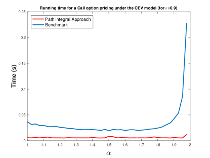
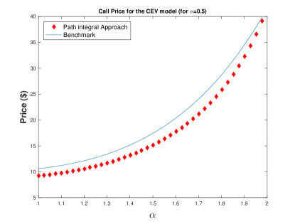
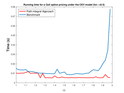
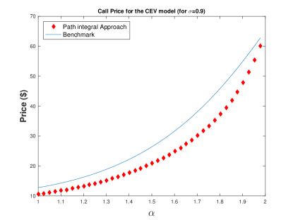
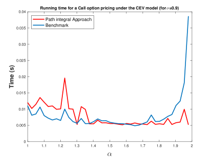
Firstly, we consider a maturity equal to six months. In Table 1 both the pricing and computational time are reported. We can see that the path integral method has similar pricing values but with a clear advantage in the running time. The times observed in the Table 1 for the proposed method of path integral are always lower to 0.008 seconds; however for the non-central chi-square approach the times are at least greater in one order of magnitude with a increase when the elasticity parameter is higher.

$\sigma$	$\alpha$	Path Integral		Benchmark
		Pricing ($\$$)	Running Time (s)	Pricing $(\$)$	Running Time (s)
$20\%$	1	4.4289e-08	0.0079	4.6567e-08	0.1595
	1.45	0.0580	0.0064	0.0600	0.0886
	1.9	1.8505	0.0060	1.8706	0.2101
$50\%$	1	0.0259	0.0078	0.0583	0.0275
	1.45	1.3437	0.0079	1.4181	0.0480
	1.9	8.0777	0.0059	8.2636	0.0603
$90\%$	1	0.3847	0.0059	0.4148	0.0307
	1.45	3.9003	0.0077	4.2358	0.0236
	1.9	16.4965	0.0074	17.1870	0.0413

Table 1: Comparison of pricing and computational time for a Call option for some values of $\sigma$ and $\alpha$, using $T=0.5$, $S_{0}=100$ and $E=110$

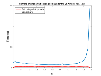
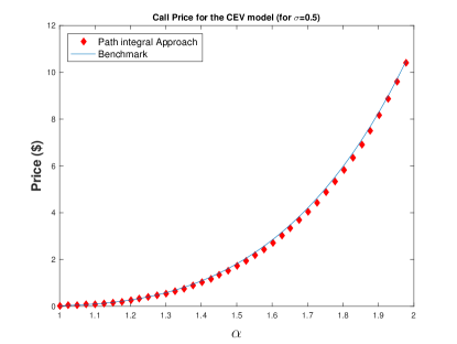
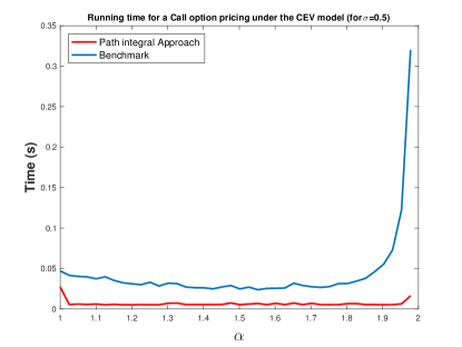
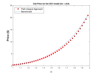
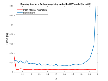
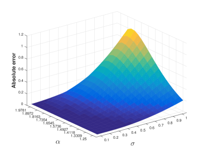
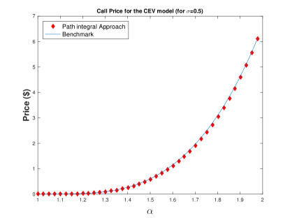
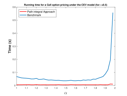
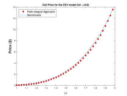
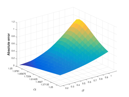
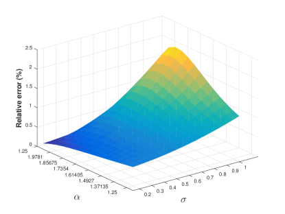
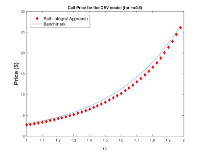
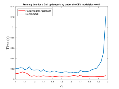
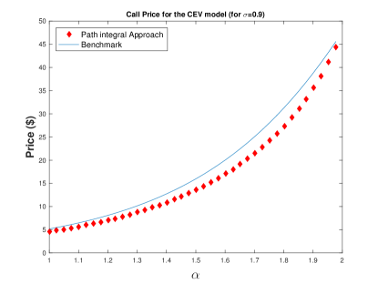
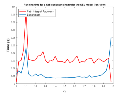
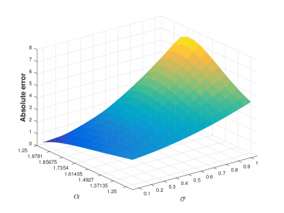
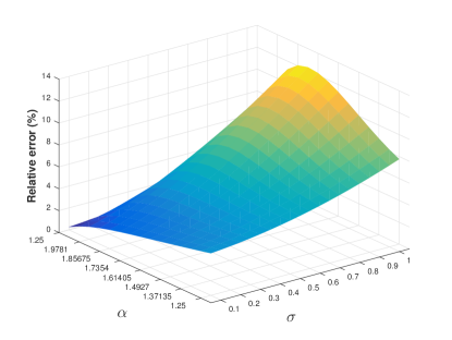
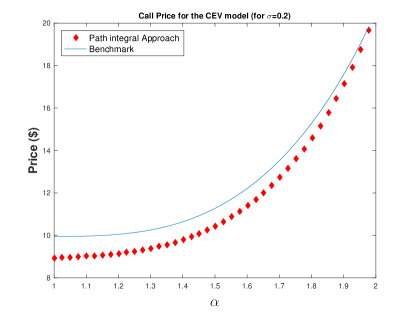
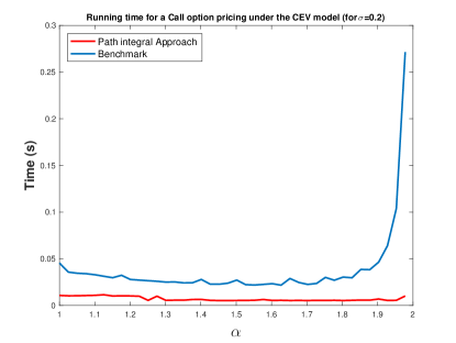
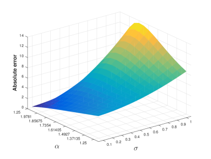
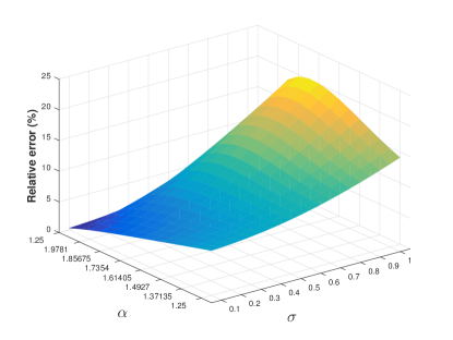
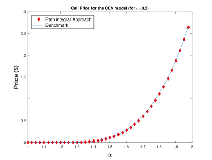
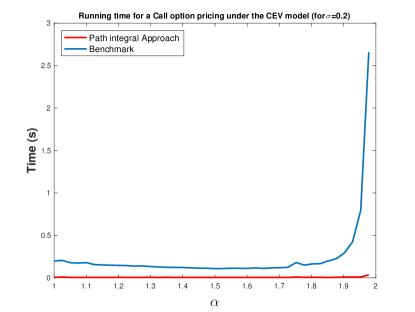
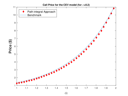
For a clearer and complete view, we present the continuous results in Figs. 1, 2 and 3 The pricing and the running time are showed for both models sweeping on values of $\alpha$. The figures confirm the observed concussions in Table 1 in the sense that the running times of the proposed method of path integral are significantly lower (right-hand side figures) than the traditional solution methodology for the CEV model, especially when $\alpha$ tends to 2 where the time of the benchmark method rises considerably. In terms of the accuracy, we can see that the path integral method fits very well in all cases. In order to have an estimation of the path integral approach, in the Fig. 4 the absolute and relative errors are shown for several values of $\alpha$ and $\sigma$. Always, the relative relative error is no longer that 10% for the assumed parameters.

(a) Option Pricing

(b) Running time

Figure 1: Pricing and computational time for a Call option using $\sigma=$20%, $T=0.5$, $r=0.05$, $S_{0}=100$ and $E=110$

(a) Option Pricing

(b) Running time

Figure 2: Pricing and computational time for a Call option using $\sigma=$50%, $T=0.5$, $r=0.05$, $S_{0}=100$ and $E=110$

(a) Option Pricing

(b) Running time

Figure 3: Pricing and computational time for a Call option using $\sigma=$90%, $T=0.5$, $r=0.05$, $S_{0}=100$ and $E=110$

(a) Absolute error

(b) Relative error

Figure 4: Absolute and relative error of of the path integral approach with $T=0.5$, $r=0.05$, $S_{0}=100$ and $E=110$

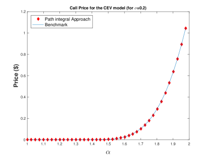
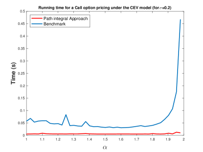
If we use a lower time to maturity (three months) the results in terms of computational time are very similar to the case $T=0.5$, and the fit is still good too. In fact, for lower maturity the path integral method performs better because the error is no greater than 2%. This is showed from Fig. 5 to Fig. 8.

(a) Option Pricing

(b) Running time

Figure 5: Pricing and computational time for a Call option using $\sigma=$20%, $T=0.25$, $r=0.05$, $S_{0}=100$ and $E=110$

(a) Option Pricing

(b) Running time

Figure 6: Pricing and computational time for a Call option using $\sigma=$50%, $T=0.25$, $r=0.05$, $S_{0}=100$ and $E=110$

(a) Option Pricing

(b) Running time

Figure 7: Pricing and computational time for a Call option using $\sigma=$90%, $T=0.25$, $r=0.05$, $S_{0}=100$ and $E=110$

(a) Absolute error

(b) Relative error

Figure 8: Absolute and relative error of of the path integral approach with $T=0.25$, $r=0.05$, $S_{0}=100$ and $E=110$

For greater times to maturity, we have a change in the results, indicating the limits of the semiclassical approximation. For a two years maturity Figs. 9-12 we find results very similar to that of the previous cases, but with a more deviation in the pricing (absolute error). Still, the relative error remains lower than 12%. However the figures show an increase in the running time, being comparable the times of both approaches, specially when the volatility rises and the elasticity is low. This fact is confirmed when we use a maturity equals to 4 years. Indeed, the computational cost increase, being the proposed method still competitive for higher $\alpha$. In the same way, the pricing error goes up, despite the fact that the relative error remains under 20%.

(a) Option Pricing

(b) Running time

Figure 9: Pricing and computational time for a Call option using $\sigma=$20%, $T=2$, $r=0.05$, $S_{0}=100$ and $E=110$

(a) Option Pricing

(b) Running time

Figure 10: Pricing and computational time for a Call option using $\sigma=$50%, $T=2$, $r=0.05$, $S_{0}=100$ and $E=110$

(a) Option Pricing

(b) Running time

Figure 11: Pricing and computational time for a Call option using $\sigma=$90%, $T=2$, $r=0.05$, $S_{0}=100$ and $E=110$

(a) Absolute error

(b) Relative error

Figure 12: Absolute and relative error of of the path integral approach with $T=2$, $r=0.05$, $S_{0}=100$ and $E=110$

(a) Option Pricing

(b) Running time

Figure 13: Pricing and computational time for a Call option using $\sigma=$20%, $T=4$, $r=0.05$, $S_{0}=100$ and $E=110$

(a) Option Pricing

(b) Running time

Figure 14: Pricing and computational time for a Call option using $\sigma=$50%, $T=4$, $r=0.05$, $S_{0}=100$ and $E=110$

(a) Option Pricing

(b) Running time

Figure 15: Pricing and computational time for a Call option using $\sigma=$90%, $T=4$, $r=0.05$, $S_{0}=100$ and $E=110$

(a) Absolute error

(b) Relative error

Figure 16: Absolute and relative error of the path integral approach with $T=4$, $r=0.05$, $S_{0}=100$ and $E=110$

6 Summary and further research

In this paper, a new numerical method for computing the CEV model was developed. In particular, this new approach was based on the semiclassical approximation of Feynman’s path integral model. This formulation dealt with some of the limitations of the conventional approach based on the non-central chi-squared distribution.

The experimental results showed a good fit between the new proposed method and the traditional methodology (setting the former as benchmark), and also a lower computational cost, measured as the running time of each model.

We analyze several hypothetical scenarios, using different maturities, volatilities and elasticities. In most cases, the running time is one order of magnitude lower than the benchmark, but if the elasticity tends to one, this difference is higher. As an accuracy measure the absolute and relative error are computed. For the range $10\%<\sigma<100\%$ and $1.25<\alpha<1.97$ the relative error is below than 20% in all the cases. Nevertheless, for short maturities and lower volatilities, the error decreases considerably, coming to be less than 10% for small maturities (under 2% for T=0.25!) and for $\sigma<50$.

The main remark is that this novel methodology allow to evaluate an European contract under the CEV model computing only an integral without any complex numerically method. The accuracy and efficiency of this method, positions it as a great competitor for the conventional method based on the non-central chi-squared distribution.

In terms of future research, a natural first extension of the paper is to adapt the proposed methodology to American options. Also, the pricing of exotic options would be a good target. Another interesting research line is to apply the semiclassical approximation of Feynman’s path integral model to more sophisticated stochastic volatility models such as: Heston, SABR or GARCH type models, where the traditional current solutions are much more complicated than that of the CEV model, and hence the potential value added of this methodology could be greater.

References

• [1] Fischer Black and Myron Scholes. The pricing of options and corporate liabilities. Journal of Political Economy, 81(3):637–654, 1973.
• [2] Geert Bekaert and Guojun Wu. Asymmetric volatility and risk in equity markets. The review of financial studies, 13(1):1–42, 2000.
• [3] Tim Bollerslev, Julia Litvinova, and George Tauchen. Leverage and volatility feedback effects in high-frequency data. Journal of Financial Econometrics, 4(3):353–384, 2006.
• [4] Mark Rubinstein. Nonparametric tests of alternative option pricing models using all reported trades and quotes on the 30 most active cboe option classes from august 23, 1976 through august 31, 1978. The Journal of Finance, 40(2):455–480, 1985.
• [5] Jens Carsten Jackwerth and Mark Rubinstein. Recovering probability distributions from option prices. The Journal of Finance, 51(5):1611–1631, 1996.
• [6] Robert F Engle. Autoregressive conditional heteroscedasticity with estimates of the variance of united kingdom inflation. Econometrica: Journal of the Econometric Society, pages 987–1007, 1982.
• [7] Tim Bollerslev, Ray Y Chou, and Kenneth F Kroner. Arch modeling in finance: A review of the theory and empirical evidence. Journal of econometrics, 52(1-2):5–59, 1992.
• [8] Eric Ghysels, Andrew C. Harvey, and Eric Renault. Stochastic volatility. In G.S. Maddala and C.R. Rao, editors, Statistical Methods in Finance, volume 14 of Handbook of Statistics, chapter 5, pages 119 – 191. Elsevier, 1996.
• [9] Neil Shephard and Torben G Andersen. Stochastic volatility: origins and overview. In Thomas Mikosch, Jens-Peter Kreiß, Richard A. Davis, and Torben Gustav Andersen, editors, Handbook of Financial Time Series, pages 233–254. Springer, Berlin, Heidelberg, 2009.
• [10] David G Hobson and Leonard CG Rogers. Complete models with stochastic volatility. Mathematical Finance, 8(1):27–48, 1998.
• [11] John C Cox. Notes on option pricing i: Constant elasticity of variance diffusions. Working paper, Stanford University, 1975.
• [12] John C Cox. The constant elasticity of variance option pricing model. The Journal of Portfolio Management, 23(5):15–17, 1996.
• [13] Stan Beckers. The constant elasticity of variance model and its implications for option pricing. The Journal of Finance, 35(3):661–673, 1980.
• [14] Mark Schroder. Computing the constant elasticity of variance option pricing formula. the Journal of Finance, 44(1):211–219, 1989.
• [15] Dmitry Davydov and Vadim Linetsky. Pricing and hedging path-dependent options under the cev process. Management science, 47(7):949–965, 2001.
• [16] Min Chen. Equity volatility smile and skew under a cev-based structural leverage model. Applied Mathematics & Information Sciences, 9(3):1095–1104, 2015.
• [17] James D MacBeth and Larry J Merville. Tests of the black-scholes and cox call option valuation models. The Journal of Finance, 35(2):285–301, 1980.
• [18] David C Emanuel and James D MacBeth. Further results on the constant elasticity of variance call option pricing model. Journal of Financial and Quantitative Analysis, 17(4):533–554, 1982.
• [19] Alan L Tucker, David R Peterson, and Elton Scott. Tests of the black-scholes and constant elasticity of variance currency call option valuation models. Journal of Financial Research, 11(3):201–214, 1988.
• [20] Beni Lauterbach and Paul Schultz. Pricing warrants: An empirical study of the black-scholes model and its alternatives. The Journal of Finance, 45(4):1181–1209, 1990.
• [21] VK Singh and N Ahmad. Forecasting performance of constant elasticity of variance model: Empirical evidence from india. International Journal of Applied Economics and Finance, 5(1):87–96, 2011.
• [22] KC Yuen, H Yang, and KL Chu. Estimation in the constant elasticity of variance model. British Actuarial Journal, 7(2):275–292, 2001.
• [23] Ying-Lin Hsu, TI Lin, and CF Lee. Constant elasticity of variance (cev) option pricing model: Integration and detailed derivation. Mathematics and Computers in Simulation, 79(1):60–71, 2008.
• [24] Manuela Larguinho, José Carlos Dias, and Carlos A Braumann. On the computation of option prices and greeks under the cev model. Quantitative Finance, 13(6):907–917, 2013.
• [25] Nawdha Thakoor, Désiré Yannick Tangman, and Muddun Bhuruth. A new fourth-order numerical scheme for option pricing under the cev model. Applied Mathematics Letters, 26(1):160–164, 2013.
• [26] Nawdha Thakoor, Désiré Yannick Tangman, and Muddun Bhuruth. Fast valuation of cev american options. Wilmott, 2015(75):54–61, 2015.
• [27] Richard Lu and Yi-Hwa Hsu. Valuation of standard options under the constant elasticity of variance model. International Journal of Business and Economics, 4(2):157, 2005.
• [28] Rajae Aboulaich, Abdelilah Jraifi, and Ibtissam Medarhri. Stochastic runge kutta methods with the constant elasticity of variance (cev) diffusion model for pricing option. International journal of mathematical analysis, 8(18):849–856, 2014.
• [29] Aricson Cruz and José Carlos Dias. The binomial cev model and the greeks. Journal of Futures Markets, 37(1):90–104, 2017.
• [30] AE Lindsay and DR Brecher. Simulation of the cev process and the local martingale property. Mathematics and Computers in Simulation, 82(5):868–878, 2012.
• [31] Sang-Hyeon Park and Jeong-Hoon Kim. Asymptotic option pricing under the cev diffusion. Journal of Mathematical Analysis and Applications, 375(2):490–501, 2011.
• [32] Stefano Pagliarani and Andrea Pascucci. Analytical approximation of the transition density in a local volatility model. Central European Journal of Mathematics, 10(1):250–270, 2012.
• [33] Vladislav Krasin, Ivan Smirnov, and Alexander Melnikov. Approximate option pricing and hedging in the cev model via path-wise comparison of stochastic processes. Annals of Finance, pages 1–15, 2017.
• [34] Vadim Linetsky. The path integral approach to financial modeling and options pricing. Computational Economics, 11(1):129–163, 1997.
• [35] Guido Montagna, Oreste Nicrosini, and Nicola Moreni. A path integral way to option pricing. Physica A: Statistical Mechanics and its Applications, 310(3):450–466, 2002.
• [36] G Bormetti, Guido Montagna, N Moreni, and Oreste Nicrosini. Pricing exotic options in a path integral approach. Quantitative Finance, 6(1):55–66, 2006.
• [37] Belal E Baaquie. Quantum finance: Path integrals and Hamiltonians for options and interest rates. Cambridge University Press, 2007.
• [38] D Lemmens, M Wouters, J Tempere, and S Foulon. Path integral approach to closed-form option pricing formulas with applications to stochastic volatility and interest rate models. Physical Review E, 78(1):016101, 2008.
• [39] Jeroen PA Devreese, Damiaan Lemmens, and Jacques Tempere. Path integral approach to asian options in the black–scholes model. Physica A: Statistical Mechanics and its Applications, 389(4):780–788, 2010.
• [40] Mauricio Contreras, Rely Pellicer, Marcelo Villena, and Aaron Ruiz. A quantum model of option pricing: When black–scholes meets schrödinger and its semi-classical limit. Physica A: Statistical Mechanics and its Applications, 389(23):5447–5459, 2010.
• [41] Mauricio Contreras. Stochastic volatility models at ρ𝜌\rho=±plus-or-minus\pm1 as second class constrained hamiltonian systems. Physica A: Statistical Mechanics and its Applications, 405:289–302, 2014.
• [42] Zura Kakushadze. Path integral and asset pricing. Quantitative Finance, 15(11):1759–1771, 2015.
• [43] Richard Phillips Feynman. Space-time approach to non-relativistic quantum mechanics. Reviews of Modern Physics, 20(2):367, 1948.
• [44] Richard P Feynman and Albert R Hibbs. Quantum mechanics and path integrals. Courier Corporation, Mineola, NY, 2010.
• [45] Christian Grosche and Frank Steiner. Handbook of Feynman Path Integrals, volume 145 of Springer Tracts in Modern Physics. Springer, 1998.
• [46] Paul A. M. Dirac. The lagrangian in quantum mechanics. Phys. Z. Sowjetunion, 3(64):64–72, 1933.
• [47] Rf Rajaraman. Some non-perturbative semi-classical methods in quantum field theory (a pedagogical review). Physics Reports, 21(5):227–313, 1975.
• [48] Thijs Koeling and RA Malfliet. Semi-classical approximations to heavy ion scattering based on the feynman path-integral method. Physics Reports, 22(4):181–213, 1975.
• [49] Masud Chaichian and A Demichev. Path Integrals in Physics: Stochastic Processes and Quantum Mechanics. Institute of Physics, 2001.
• [50] Cécile Morette. On the definition and approximation of feynman’s path integrals. Physical Review, 81(5):848, 1951.
• [51] Cécile DeWitt-Morette. Feynman path integrals. Communications in Mathematical Physics, 37(1):63–81, 1974.
• [52] Ph Choquard and F Steiner. The story of van vleck’s and morette van hove’s determinants. Helvetica Physica Acta, 69(5-6):636–654, 1996.
• [53] John H Van Vleck. The correspondence principle in the statistical interpretation of quantum mechanics. Proceedings of the National Academy of Sciences, 14(2):178–188, 1928.
• [54] Rangarajan K Sundaram. Equivalent martingale measures and risk-neutral pricing: An expository note. The Journal of Derivatives, 5(1):85–98, 1997.
• [55] Hannen Risken. The Fokker–Planck equation, volume 18 of Springer series in synergetics. Springer, first edition, 1984.
• [56] Belal E Baaquie, Claudio Coriano, and Marakani Srikant. Hamiltonian and potentials in derivative pricing models: exact results and lattice simulations. Physica A: Statistical Mechanics and its Applications, 334(3):531–557, 2004.
• [57] Dirk Veestraeten. On the multiplicity of option prices under cev with positive elasticity of variance. Review of Derivatives Research, 20(1):1–13, 2017.
• [58] Freddy Delbaen and Hiroshi Shirakawa. A note on option pricing for the constant elasticity of variance model. Asia-Pacific Financial Markets, 9(2):85–99, 2002.
• [59] Matthew Lorig. The exact smile of certain local volatility models. Quantitative Finance, 13(6):897–905, 2013.
• [60] John C Cox and Stephen A Ross. The valuation of options for alternative stochastic processes. Journal of financial economics, 3(1-2):145–166, 1976.
• [61] George E Uhlenbeck and Leonard S Ornstein. On the theory of the brownian motion. Physical review, 36(5):823, 1930.
• [62] Lawrence F Shampine. Vectorized adaptive quadrature in matlab. Journal of Computational and Applied Mathematics, 211(2):131–140, 2008.