Sobolev spaces with non-Muckenhoupt weights, fractional elliptic operators, and applications

Abstract

We propose a new variational model in weighted Sobolev spaces with non-standard weights and applications to image processing. We show that these weights are, in general, not of Muckenhoupt type and therefore the classical analysis tools may not apply. For special cases of the weights, the resulting variational problem is known to be equivalent to the fractional Poisson problem. The trace space for the weighted Sobolev space is identified to be embedded in a weighted $L^{2}$ space. We propose a finite element scheme to solve the Euler-Lagrange equations, and for the image denoising application we propose an algorithm to identify the unknown weights. The approach is illustrated on several test problems and it yields better results when compared to the existing total variation techniques.

35S15, 26A33, 65R20, 65N30

1 Introduction

In this paper we consider weighted Sobolev spaces where the weight $w$ is not necessarely of Muckenhoupt type, and an associated variational model with concrete applications to image processing that shows advantageous features of such weights. The particular weights $w$ that we consider in this paper are closely related to fractional Sobolev spaces of differentiability order $s\in(0,1)$ and the fractional spectral Laplacian $(-\Delta)^{s}$, and are further motivated by considering a spatially dependent order $x\mapsto s(x)$.

Weighted Sobolev spaces have been a topic of intensive study for around 60 years with a variety of focuses; we refer the readers to the monographs [17, 15, 25] and references within, and further [28, 11, 27, 16, 20] for an introduction to the subject. In particular, a source of interest for such spaces is that they represent the correct solution space for several degenerate elliptic partial differential equations ([17]) and problems in potential theory ([25]). Recently, the topic has received a new impulse mainly associated with the extension result of Caffarelli-Silvestre; [5] (Stinga-Torrea; [24]) for fractional elliptic partial differential operators. In this setting, for example, the solution to $(-\Delta)^{s}u=f$ in the fractional Sobolev space $H^{s}(\Omega)$ endowed with zero boundary conditions, can be equivalently obtained as (the restriction to $\Omega$ of) the solution of a PDE with a non-fractional elliptic operator in a weighted Sobolev space with weight $w(x,y)=y^{1-2s}$ in the extended domain $\mathcal{C}=\{(x,y)\in\Omega\times(0,+\infty)\}$.

The type of weights $w$ that have been more thoroughly studied correspond to two main classes: 1) weights belonging to some Muckenhoupt class; see [11, 27] and 2) composition of functions (mainly power functions) with the distance function to a particular set; see [15, 20]. In these cases, several important questions like density of smooth functions and characterization of traces have been, at least partially, answered; see [28, 11, 15, 20]. In this paper we consider weights of the type $w(x,y)=y^{1-2s(x)}$ on $\mathcal{C}=\{(x,y)\in\Omega\times(0,+\infty)\}$, which are, in general, neither of 1) or 2) type.

The variational problem of interest in this paper is closely related to fractional elliptic operators. The spike of research interest on problems with this type of operators is mainly due to the results from Caffarelli and collaborators; see [24, 5, 6]. Following the renowned results in [5], a large number of contributions on modeling, numerical methods, applications, regularity results, different boundary conditions, and control problems, among others have been considered.

Recently, for image denoising a model was proposed in [1]. The variational problem can be formulated in our setting as

(1.1) $$\min_{u}\frac{1}{2}\|(-\Delta)^{\frac{s}{2}}v\|_{L^{2}(\Omega)}^{2}+\frac{\zeta}{2}\|v-f\|^{2}_{L^{2}(\Omega)},$$

where $(-\Delta)^{s}$ denotes the fractional power of the Laplacian with zero Neumann boundary conditions and $s\in(0,1)$; see [6, 2]. Additionally, $\zeta>0$ is a given constant, and $f=u_{\mathrm{true}}+\mathrm{noise}$ where $u_{\mathrm{true}}$ is the desired target of the optimization procedure. The choice of $s$ has a direct consequence on the global regularity of the solution to problem (1.1). However, it is desirable, from the reconstruction point of view, that the regularity of the solution to (1.1) is low in places in $\Omega$ where edges or discontinuities are present in $u_{\mathrm{true}}$, and that is high in places where $u_{\mathrm{true}}$ is smooth or contains homogeneous features. Hence, it is of interest to consider (1.1) where $s\mathrel{\mathop{\mathchar 58\relax}}\Omega\to[0,1]$ is not a constant. The first main roadblock in letting $s$ to be spatially dependent is the fact that there is no obvious way to define $(-\Delta)^{s(x)}$. In fact we will not attempt to do so in this paper, we leave this as an open question. Instead of (1.1) we consider the following variational problem:

(1.2) $$\min_{u}\frac{1}{2}\int_{\mathcal{C}}y^{1-2s(x)}\left(\theta|u|^{2}+|\nabla u|^{2}\right)\>\mathrm{d}x\>\mathrm{d}y+\frac{\mu}{2}\int_{\Omega}s(x)^{2}|u(x,0)-f|^{2}\>\mathrm{d}x,$$

where $\mathcal{C}=\{(x,y)\in\Omega\times(0,+\infty)\}$, $0<\theta\ll 1$, $\mu>0$ is a given constant, and $u(x,0)$ stands for the trace of $u$ at $\Omega\times\{0\}$. For the solution $u$ of this optimization problem, we expect that $u(\cdot,0)\simeq u_{\mathrm{true}}$. This problem is the focus of the present paper and the full motivational link between the problems (1.1) and (1.2), is given in the following section.

We next summarize the main contributions of this paper and discuss how the paper is organized in what follows.

In section 1.1, we provide a rigorous motivation for the study of problem (1.2) by showing that (1.2) represents a generalization of (1.1), after using the Caffarelli-Silvestre extension, in the case of $s$ non-constant. For a constant $s\in(0,1)$ the definition of fractional Laplacian in terms of the Caffarelli-Silvestre or the Stinga-Torrea extension is by now well-known. However such a result remains open when $s(x)\in[0,1]$ for $x\in\Omega$. Towards this end we emphasize that we have formulated our problem (1.2) on an unbounded domain $\mathcal{C}=\Omega\times(0,+\infty)$, and not directly over $\Omega$.

In order to handle varying $s$ in space, for almost all (f.a.a) $x\in\Omega$ we assume $s(x)\in[0,1]$, and consider weighted Sobolev with weights $w(x,y)=y^{1-2s(x)}$ on $\mathcal{C}$. This class of Sobolev spaces is studied in section 2 and we establish also two fundamental results. The first one is that since we allow $s(x)=0$, for some $x\in\Omega$, the weight $y^{1-2s(x)}$ is not, in general, in the Muckenhoupt class $A_{2}$ (cf. Proposition 2.1). Due to the lack of this $A_{2}$ property we cannot use some of the existing machinery on weighted Sobolev spaces. In particular, the density of smooth functions is not always given in weighted spaces in the absence of the properties inherited by the Muckenhoupt class. The second important result of section 2 characterizes the trace space for this class of weighted Sobolev spaces, this is given in Theorem 2.3, and it is established that the trace space embeds continuously on the $s$-weighted $L^{2}$ space. In addition, we give examples of functions with discontinuous traces in Example 2.

In section 3, we establish properties for the variational problem of interest (1.2), and a procedure for the selection of the function $s$. We finalize the paper with section 4, where we develop a discretization scheme, and provide numerical tests that positively compared with other methods for image reconstruction. In particular, in section 4.1 we introduce a finite element method for (1.6) on a bounded domain $\mathcal{C}_{\tau}\mathrel{\mathop{\mathchar 58\relax}}=\mathcal{C}\times(0,\tau)$. Since our targeted application is image denosing so we first state an Algorithm to determine $s$ in Algorithm 1. We apply this approach to several prototypical examples in section 5. In all cases we obtain better results when compared to the Total Variation (TV) approach.

1.1 Motivation and some notation

Our point of departure for motivation to study the proposed variational model (and associated function space properties) is Figure 1

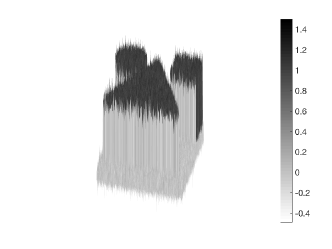
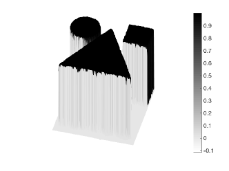
Figure 1: Example 1. Left panel: noisy image. Middle panel: reconstruction using Total Variation (TV) approach [8]. Right panel: reconstruction using the approach introduced in this paper.

where the left panel shows a noisy image, the middle panel shows the reconstruction using the Total Variation (TV) model, explained in what follows, (we use piecewise linear finite element discretization for the TV model and we stop the algorithm when the relative error between the consecutive iterates is smaller than $1e$-8.), and the rightmost panel shows the reconstruction using the new framework introduced in this paper and briefly explained in this section. The Rudin-Osher-Fatemi (ROF) model, also called the TV model, was introduced in [23] and is given by

(1.3) $$\min_{u\in{\rm BV}(\Omega)}\int_{\Omega}|Du|+\frac{\zeta}{2}\|u-f\|^{2}_{L^{2}(\Omega)},$$

where $\Omega\subset\mathbb{R}^{N}$ with $N\geq 1$ is a open bounded Lipschitz domain, and $f\in L^{2}(\Omega)$ is given by $f=u_{\mathrm{true}}+\xi$, where $\xi$ is the “noise”. Moreover, $\zeta>0$ is the regularization parameter, and $\int_{\Omega}|Du|$ denotes the total variation seminorm of $u$ on $\Omega$ ; see [4]. The parameter $\zeta>0$ in Figure 1 is chosen so that it maximizes a weighted sum of the Peak Signal to Noise Ratio (PSNR) and the Structural Similarity index (SSIM); as in [14]. These two indexes measure with different criteria how close the solution $u_{\rm tv}$ to (1.3) is to $u_{\mathrm{true}}$; see [26]. The fundamental question in such applications is: Is it possible to capture the sharp transitions (edges) across the interfaces while removing the undesirable noise from remainder of the domain. Such a question is not limited to image denoising but is fundamental to many applications in science and engineering. For instance multiphase flows (diffuse interface models), fracture mechanics, image segmentation etc. Even though the ROF model has been extremely successful in practice, two main drawbacks are observed in reconstructions: 1) loss of contrast is always present 2) some corners tend to be rounded (cf. Figure 1, middle panel).

The problem (1.1) proposed in [1] is obtained if $\int_{\Omega}|D\cdot|$ is replaced by $\frac{1}{2}\|(-\Delta)^{\frac{s}{2}}\cdot\|_{L^{2}(\Omega)}^{2}$ where $(-\Delta)^{s}$ denotes the fractional powers of the Laplacian with zero Neumann boundary conditions, for $s\in(0,1)$. Solutions to (1.1) are given in $H^{s}(\Omega)$, the fractional Sobolev space given by

$$H^{s}(\Omega)=\left\{v\in L^{2}(\Omega)\mathrel{\mathop{\mathchar 58\relax}}\int_{\Omega}\int_{\Omega}\frac{|v(x)-v(y)|^{2}}{|x-y|^{n+2s}}\>\mathrm{d}x\>\mathrm{d}y<+\infty\right\}.$$

The minimization problem (1.1) is appealing, in contrast to (1.3), as the Euler-Lagrange equations are linear in $u$, i.e., if $u$ solves (1.1), then equivalently it solves

(1.4) $$\langle(-\Delta)^{s}u,v\rangle+\zeta(u-f,v)=0,$$

for all $v\in H^{s}(\Omega)$. Both (1.1) and hence (1.4) have unique solutions in $H^{s}(\Omega)$. This can be easily deduced from the definition of Neumann fractional Laplacian and the equivalence between the spectral and $H^{s}(\Omega)$-norms (cf. [2, Remark 2.5] and [6]). The $H^{s}(\Omega)$ space further provides flexibility in terms of the regularity by choosing $s$ appropriately.

The Caffarelli-Silvestre (or Stinga-Torrea) extension technique establishes that if $u\in H^{s}(\Omega)$ solves (1.4), then there exists $\mathcal{U}\in H(\mathcal{C};y^{1-2s})$ where $H(\mathcal{C};y^{1-2s})$ is the weighted $H^{1}$ Sobolev space on $\mathcal{C}\mathrel{\mathop{\mathchar 58\relax}}=\Omega\times(0,\infty)$ with weight $w(x,y)=y^{1-2s}$, $(x,y)\in\mathcal{C}$ (see the following section for more details), such that $\mathrm{tr}_{\Omega}\>\mathcal{U}=u$, where $\mathrm{tr}_{\Omega}\>$ operator is the restriction of the trace map to $\Omega$, and $\mathcal{U}$ solves

(1.5) $$\begin{aligned} \int_{\mathcal{C}}y^{1-2s}\nabla\mathcal{U}\cdot\nabla\mathcal{W}&\>\mathrm{d}x\>\mathrm{d}y+d_{s}\zeta\int_{\Omega}(\mathrm{tr}_{\Omega}\>\mathcal{U}-f)\>\mathrm{tr}_{\Omega}\>\mathcal{W}\>\>\mathrm{d}x=0,\end{aligned}$$

for all $\mathcal{W}\in H(\mathcal{C};y^{1-2s})$, where $d_{s}=2^{1-2s}\frac{\Gamma(1-s)}{\Gamma(s)}$. Therefore, for $s$ a constant such that $s(x)=s\in(0,1)$ for all $x\in\Omega$, $\theta=0$ and $\zeta\mathrel{\mathop{\mathchar 58\relax}}=\mu s^{2}d_{s}^{-1}$, if $\mathcal{U}$ solves (1.2), then it equivalently solves (1.5). This establishes the connection of (1.2) with (1.4), and hence with (1.1).

Further, if $s(\cdot)$ is not a constant and $s\mathrel{\mathop{\mathchar 58\relax}}\Omega\to[0,1]$ (with some additional assumptions made explicit in the following section), and if $\mathcal{U}\in H(\mathcal{C};y^{1-2s(x)})$ solves (1.2), then

(1.6) $$\begin{aligned} \int_{\mathcal{C}}y^{1-2s(x)}\left(\nabla\mathcal{U}\cdot\nabla\mathcal{W}+\theta\mathcal{U}\mathcal{W}\right)&\>\mathrm{d}x\>\mathrm{d}y+\mu\int_{\Omega}s(x)^{2}(\mathrm{tr}_{\Omega}\>\mathcal{U}-f)\>\mathrm{tr}_{\Omega}\>\mathcal{W}\>\>\mathrm{d}x=0,\end{aligned}$$

for all $\mathcal{W}\in H(\mathcal{C};y^{1-2s(x)})$; this is rigorously done in section 3 where the key ingredient is the characterization of $\mathrm{tr}_{\Omega}\>$ of $H(\mathcal{C};y^{1-2s(x)})$. It is clear that for $\theta\ll 1$, the above problem (whenever well-posed) represents a generalization of (1.5) and hence of (1.1).

Now we are in shape to explain Figure 1. First, note that for $s\simeq 0$, we expect low regularity of solutions, and for $s\simeq 1$ we expect higher regularity of solutions: In fact, for constant $0<s_{1}<s_{2}<1$, we observe $H^{s_{2}}(\Omega)\subset H^{s_{1}}(\Omega)$. Then, after a rough identification of edges, we choose $s$ small on edges, and large on other regions; the exact procedure is provided in section 4.2. The right image in Figure 1, is obtained via this procedure.

2 Weighted Sobolev space with variable $s$ and their traces

Let $\Omega\subset\mathbb{R}^{N}$ with $N\geq 1$ be a non-empty, open, bounded domain with Lipschitz boundary $\partial\Omega$. We denote by $\mathcal{C}\mathrel{\mathop{\mathchar 58\relax}}=\Omega\times(0,\infty)$ a semi-infinite cylinder with boundary $\partial_{L}\mathcal{C}\mathrel{\mathop{\mathchar 58\relax}}=\partial\Omega\times[0,\infty)$. With $s\mathrel{\mathop{\mathchar 58\relax}}\Omega\to\mathbb{R}$ measurable and $s(x)\in[0,1]$ for almost all $x\in\Omega$, we define

$$\delta(x)\mathrel{\mathop{\mathchar 58\relax}}=1-2s(x)\in[-1,1],\qquad\text{ and }\qquad w(x,y)\mathrel{\mathop{\mathchar 58\relax}}=y^{\delta(x)},$$

so that

(2.1) $$w,w^{-1}\in L^{1}_{\mathrm{loc}}(\mathcal{C}).$$

We denote $L^{2}(\mathcal{C};y^{\delta(x)})\mathrel{\mathop{\mathchar 58\relax}}=L^{2}(\mathcal{C};w)$, where

$$L^{2}(\mathcal{C};y^{\delta(x)})\mathrel{\mathop{\mathchar 58\relax}}=\left\{v\mathrel{\mathop{\mathchar 58\relax}}\mathcal{C}\to\mathbb{R}\mathrel{\mathop{\mathchar 58\relax}}v\text{ is measurable and }\int_{\mathcal{C}}y^{\delta(x)}|v|^{2}\>\mathrm{d}x\>\mathrm{d}y<+\infty\right\},$$

which is a well-defined weighted Lebesgue space.

For $u$ smooth, define the (extended real-valued) functional $\|\cdot\|_{H}$ as

(2.2) $$\|u\|_{H}\mathrel{\mathop{\mathchar 58\relax}}=\left(\int_{\mathcal{C}}y^{\delta(x)}\left(|u|^{2}+|\nabla u|^{2}\right)\>\mathrm{d}x\>\mathrm{d}y\right)^{\frac{1}{2}}.$$

Note that if $\|u\|_{H}<+\infty$, the value of $s$ controls how singular the function $u$ is in the neighborhood of $\Omega\times\{0\}$. Define $\mathcal{A}_{\alpha}(s)\mathrel{\mathop{\mathchar 58\relax}}=\{x\in\Omega\mathrel{\mathop{\mathchar 58\relax}}s(x)=\alpha,\>\>\text{a.e.}\}$, suppose that for $\alpha=1$ its Lebesgue measure satisfies $|\mathcal{A}_{1}(s)|>0$, and that $u$ is a constant in $\mathcal{A}_{1}(s)\times(0,h)$, then

$$\|u\|^{2}_{H}\geq|u|^{2}|\mathcal{A}_{1}(s)|\int_{0}^{h}y^{-1}\>\mathrm{d}y,$$

so that $u$ is zero in $\Omega\times(0,h)$. On the other hand, $u$ is allowed to have a more singular behaviour on $\mathcal{A}_{0}(s)$.

Consider the set

$$\mathcal{C}_{\Omega}=(\Omega\times\{0\})\cup\mathcal{C},$$

that is, $\mathcal{C}_{\Omega}$ is the open cylinder $\mathcal{C}$ together with the $\Omega$ cap, and denote by $H$, $H_{0}$, and $W$, or equivalently by $H(\mathcal{C};y^{\delta(x)})$, $H_{0}(\mathcal{C};y^{\delta(x)})$, and $W(\mathcal{C};y^{\delta(x)})$, the spaces $H(\mathcal{C};w)$, $H_{0}(\mathcal{C};w)$ and $W(\mathcal{C};w)$ which are defined as

$H(\mathcal{C};w)$ is the closure of the set $K\mathrel{\mathop{\mathchar 58\relax}}=\{w\in C^{\infty}(\overline{\mathcal{C}})\mathrel{\mathop{\mathchar 58\relax}}\|w\|_{H}<+\infty\}$ with respect to the $\|\cdot\|_{H}$ norm.

$H_{0}(\mathcal{C};w)$ is the closure of the set $K_{0}\mathrel{\mathop{\mathchar 58\relax}}=\{w\in C_{c}^{\infty}(\mathcal{C}_{\Omega})\mathrel{\mathop{\mathchar 58\relax}}\|w\|_{H}<+\infty\}$ with respect to the $\|\cdot\|_{H}$ norm.

$W(\mathcal{C};w)$ is the space of maps $u\in L^{2}(\mathcal{C};y^{\delta(x)})\cap L_{\mathrm{loc}}^{1}(\mathcal{C})$ with distributional gradients $\nabla u$ that satisfy $|\nabla u|\in L^{2}(\mathcal{C};y^{\delta(x)})\cap L_{\mathrm{loc}}^{1}(\mathcal{C})$.

A few words are in order concerning the definition of $H$ given the slight difference from the existing literature: Usually, the definition of $H$ is given over the completion (of finite energy functions) of $C^{\infty}(\mathcal{C})$, in contrast to $C^{\infty}(\overline{\mathcal{C}})$, with respect to the $H$ norm; see [27]. Provided that $\partial\mathcal{C}$ is regular enough, $\mathcal{C}$ is bounded, and $w,w^{-1}$ are bounded above and below ($\epsilon>0$ away from zero) on a neighborhood of $\partial\mathcal{C}$, then the closure in the definition of $H$ can be equivalently taken with $C^{\infty}(\mathcal{C})$ or $C^{\infty}(\overline{\mathcal{C}})$, indistinctly. Since in our case the two last conditions are not satisfied, we consider $H$ the way it is defined here.

First note that since $K_{0}\subset K$, which follows from $C_{c}^{\infty}(\mathcal{C}_{\Omega})\subset C^{\infty}(\overline{\mathcal{C}})$, we have that $H_{0}\subset H$. The notation of “$H_{0}$” comes from the following: If $v\in K_{0}$, then $v|_{\partial\Omega\times\{0\}}=0$, so that restrictions of elements of $H_{0}$ to $\Omega$ have “zero boundary conditions”. In particular, in the case $s\in(0,1)$ is constant, the latter remark can be taken out of quotation marks and considered in the sense of the trace; see [7]. The condition (2.1) implies (see [27, 16]) that the space $W$ is a proper weighted Sobolev space endowed with the $H$-norm. While it holds that $H(\tilde{\mathcal{C}};\tilde{w})\subset W(\tilde{\mathcal{C}};\tilde{w})$, for general weights $\tilde{w}$ and domains $\tilde{\mathcal{C}}$, it does not necessarily hold that $H(\tilde{\mathcal{C}};\tilde{w})=W(\tilde{\mathcal{C}};\tilde{w})$. For $\tilde{w}=1$, the equality holds provided conditions on $\tilde{\mathcal{C}}$ are given, e.g., if $\tilde{\mathcal{C}}$ is bounded and has a Lipschitz boundary. A sufficient condition for $H(\tilde{\mathcal{C}};\tilde{w})=W(\tilde{\mathcal{C}};\tilde{w})$, when $\tilde{w}$ and $\tilde{\mathcal{C}}$ are benign enough, is that $\tilde{w}$ belongs to the $A_{2}(\tilde{\mathcal{C}})$ Muckenhoupt class, that is

(2.3) $$\left(\frac{1}{Q}\int_{Q}\tilde{w}\>\mathrm{d}x\>\mathrm{d}y\right)\left(\frac{1}{Q}\int_{Q}\tilde{w}^{-1}\>\mathrm{d}x\>\mathrm{d}y\right)\leq M,$$

for some $M>0$ and all open cubes $Q\subset\tilde{\mathcal{C}}$, see [25, 10]. Further, note that (2.1), does not imply (2.3). Additionally, if $0<\epsilon\leq s\leq 1-\epsilon$ a.e., then $(x,y)\mapsto y^{1-2s}$ is a Muckenhoupt $A_{2}(\mathcal{C})$ weight. However, we are particularly interested in cases where $s$ satisfies

(2.4) $$\mathrm{ess\>inf}_{x\in\Omega}s(x)=0,$$

as this will allow almost perfect approximation of functions with jump discontinuities. Remarkably enough condition (2.4) prevents $w$ to be a Muckenhoupt weight in general as we show next.

Proposition 2.1.

Suppose that for $x_{0}\in\Omega$, $s(x)\simeq|x-x_{0}|^{q}$ (locally) on $x_{0}$ for some $q>0$, that is, there exists positive constants $R_{0},M_{0},m_{0}$ such that

(2.5) $$m_{0}|x-x_{0}|^{q}\leq s(x)\leq M_{0}|x-x_{0}|^{q},$$

for all $x$ such that $|x-x_{0}|\leq R_{0}$. Then, $w\notin A_{2}(\mathcal{C})$ where $w(x,y)\mathrel{\mathop{\mathchar 58\relax}}=y^{1-2s(x)}$.

Proof 2.2.

First step. Suppose first that $x_{0}=0\in\Omega$, $s(x)=|x|^{q}$ for $x\in B_{R_{0}}(0)$, and let $Q_{R}=B_{R}(0)\times(0,y_{0})$ for $0<R\leq R_{0}<1$ and $0<y_{0}<1$.

Using cylindrical coordinates we observe

$$\int_{Q_{R}}w\>\mathrm{d}x\>\mathrm{d}y \geq C_{1}\int_{0}^{R}\int_{0}^{y_{0}}r^{N-1}y^{1-2r^{q}}\>\mathrm{d}y\>\mathrm{d}r\geq C_{2}\int_{0}^{R}r^{N-1}y_{0}^{2-2r^{q}}\>\mathrm{d}r$$

$$\geq C_{3}R^{N}y_{0}^{2},$$

where $C_{1},C_{2}$, and $C_{3}$ are positive and independent of $R$ and $y_{0}$. Similarly,

$$\int_{Q_{R}}w^{-1}\>\mathrm{d}x\>\mathrm{d}y \geq C_{1}\int_{0}^{R}\int_{0}^{y_{0}}r^{N-1}y^{-(1-2r^{q})}\>\mathrm{d}y\>\mathrm{d}r\geq C_{4}\int_{0}^{R}r^{N-1-q}y_{0}^{2r^{q}}\>\mathrm{d}r$$

$$\geq C_{5}R^{N-q}y_{0}^{2R^{q}},$$

where also $C_{4}$, and $C_{5}$ are positive and independent of $R$ and $y_{0}$. Since $|Q_{R}|\simeq R^{N}y_{0}$, we have

$$\left(\frac{1}{|Q_{R}|}\int_{Q_{R}}w\>\mathrm{d}x\>\mathrm{d}y\right)\left(\frac{1}{|Q_{R}|}\int_{Q_{R}}w^{-1}\>\mathrm{d}x\>\mathrm{d}y\right)\geq C_{6}\frac{y_{0}^{2R^{q}}}{R^{q}},$$

for some $C_{6}>0$ independent of $R$. Taking $R\downarrow 0$, we have that the L.H.S. expression is unbounded.

Second step: Consider $x_{0}\neq 0$, $s(x)\neq|x|^{q}$, and show that the above inequality holds similarly for a family of cubes $R\mapsto\tilde{Q}_{R}$.

If $x_{0}\neq 0$ and $s(x)=|x|^{q}$, then a linear change of coordinates can be performed and the proof above still holds, so the choice of $x_{0}=0$ is without loss of generality.

Additionally, let $\tilde{Q}_{R}\supset Q_{R}$ be defined as $\tilde{Q}_{R}=S_{R}(0)\times(0,y_{0})$ where $S_{R}(0)$ is the smallest square that contains $B_{R}(0)$. Hence, the quotient $|S_{R}(0)|/|B_{R}(0)|$ is independent of $R$ and for $c\mathrel{\mathop{\mathchar 58\relax}}=|\tilde{Q}_{R}|/|Q_{R}|$ we observe

$$\left(\frac{1}{|\tilde{Q}_{R}|}\int_{\tilde{Q}_{R}}w\>\mathrm{d}x\>\mathrm{d}y\right)\left(\frac{1}{|\tilde{Q}_{R}|}\int_{\tilde{Q}_{R}}w^{-1}\>\mathrm{d}x\>\mathrm{d}y\right)$$

$$\qquad\qquad\geq\frac{1}{c^{2}}\left(\frac{1}{|Q_{R}|}\int_{Q_{R}}w\>\mathrm{d}x\>\mathrm{d}y\right)\left(\frac{1}{|Q_{R}|}\int_{Q_{R}}w^{-1}\>\mathrm{d}x\>\mathrm{d}y\right).$$

Hence, by taking $R\downarrow 0$, we have that $(x,y)\mapsto y^{1-2|x|^{q}}$ is not in $A_{2}(\mathcal{C})$.

Finally, for $s(x)\neq|x|^{q}$ but when (2.5) holds true, we similarly have

$$\left(\frac{1}{|Q|}\int_{Q}w\>\mathrm{d}x\>\mathrm{d}y\right)\left(\frac{1}{|Q|}\int_{Q}w^{-1}\>\mathrm{d}x\>\mathrm{d}y\right)$$

$$\qquad\qquad\geq\tilde{c}\left(\frac{1}{|Q|}\int_{Q}\tilde{w}\>\mathrm{d}x\>\mathrm{d}y\right)\left(\frac{1}{|Q|}\int_{Q}\tilde{w}^{-1}\>\mathrm{d}x\>\mathrm{d}y\right),$$

for some $\tilde{c}>0$, where $\tilde{w}(x,y)\mathrel{\mathop{\mathchar 58\relax}}=y^{1-2|x|^{q}}$ and $w(x,y)\mathrel{\mathop{\mathchar 58\relax}}=y^{1-2s(x)}$, i.e., $w\notin A_{2}(\mathcal{C})$.

Remark 1.

Although the above result is quite general with respect of the rate of decrease of $s$, at this point, we do not know if there are continuous functions $s$ with zeros within the domain $\Omega$, for which $(x,y)\mapsto y^{1-2s(x)}$ is an element of $A_{2}(\mathcal{C})$.

The study of the trace space of $H$ is of utmost importance in what follows. In particular, we are interested in the restriction of the trace operator to $\Omega$. The paper [7] studies the trace of $H$ when $s$ is independent of $x$ and away from 0. However, that approach which is based on [18] cannot be applied here. We next prove a trace characterization result, the proof is inspired by [20] where the authors consider bounded domains and weights of distance to the boundary type.

Theorem 2.3.

Let $s$ be such that its zero set $\mathcal{A}_{0}(s)\mathrel{\mathop{\mathchar 58\relax}}=\{x\in\Omega\mathrel{\mathop{\mathchar 58\relax}}s(x)=0,\>\>\text{a.e.}\}$ has zero measure. Then, there exist a unique bounded linear trace operator

$$\mathrm{tr}_{\Omega}\>\mathrel{\mathop{\mathchar 58\relax}}H,H_{0}\rightarrow L^{2}(\Omega;(1-\delta(x))^{2})=L^{2}(\Omega;s(x)^{2})$$

such that $\mathrm{tr}_{\Omega}\>(u)=u|_{\Omega\times\{0\}}$, for all $u\in H\cap C^{\infty}(\overline{\mathcal{C}})$, and hence also for all $u\in H_{0}\cap C_{c}^{\infty}(\mathcal{C}_{\Omega})$.

Proof 2.4.

Consider $u\in H$ such that $u\in C^{\infty}(\overline{\mathcal{C}})$. Let $(x,y)\in\overline{\mathcal{C}}$ and $x\notin\mathcal{A}_{0}(s)$, then it follows that

$$u(x,y)=u(x,0)+\int_{0}^{1}yD_{N+1}u(x,ty)\>\mathrm{d}t,$$

where $D_{N+1}$ corresponds to the partial derivative with respect to the $N+1$ coordinate. Then, multiplication by $y^{\delta(x)/2}$ and integrating from $0$ to $\sigma>0$ with respect to $y$ leads to

$$|u(x,0)|\int_{0}^{\sigma}y^{\delta(x)/2}\>\mathrm{d}y\leq\int_{0}^{\sigma}|u(x,y)|y^{\delta(x)/2}\>\mathrm{d}y+\int_{0}^{\sigma}\int_{0}^{1}y|D_{N+1}u(x,ty)|y^{\delta(x)/2}\>\mathrm{d}y\>\mathrm{d}t.$$

Note that $\delta(x)/2\leq 1/2$ and suppose without loss of generality $0<\sigma\leq 1$, then $y^{1/2}\leq y^{\delta(x)/2}$ for all $y\in(0,\sigma)$. Therefore,

$$\frac{2}{3}\sigma^{3/2}\leq\int_{0}^{\sigma}y^{\delta(x)/2}\>\mathrm{d}y,$$

and hence,

(2.6) $$|u(x,0)|\leq I_{1}+I_{2},$$

for

$$I_{1}\mathrel{\mathop{\mathchar 58\relax}}=\frac{3}{2}\sigma^{-3/2}\int_{0}^{\sigma}|u(x,y)|y^{\delta(x)/2}\>\mathrm{d}y,\;\;I_{2}=\frac{3}{2}\sigma^{-3/2}\int_{0}^{1}\int_{0}^{\sigma}y|D_{N+1}u(x,ty)|y^{\delta(x)/2}\>\mathrm{d}y\>\mathrm{d}t,$$

and where we have used Tonelli’s theorem to switch the order of integration in the expression that orginates $I_{2}$.

Hölder’s inequality implies that, for $I_{1}$, we have

$$I_{1} \leq\frac{3}{2}\sigma^{-\frac{3}{2}}\left(\int_{0}^{\sigma}\>\mathrm{d}y\right)^{\frac{1}{2}}\left(\int_{0}^{\sigma}|u(x,y)|^{2}y^{\delta(x)}\>\mathrm{d}y\right)^{\frac{1}{2}}\leq\frac{3}{2}\sigma^{-1}\left(\int_{0}^{R}|u(x,y)|^{2}y^{\delta(x)}\>\mathrm{d}y\right)^{\frac{1}{2}},$$

for any $R\geq\sigma$.

Further, for $I_{2}$ consider the change of variable $z=ty$ and again by Hölder’s inequality we observe:

$$I_{2}\leq\frac{3}{2}\sigma^{-\frac{1}{2}}\int_{0}^{1}\int_{0}^{\sigma t}|D_{N+1}u(x,z)|z^{\frac{\delta(x)}{2}}t^{-1-\frac{\delta(x)}{2}}\>\mathrm{d}z\>\mathrm{d}t$$

$$\leq\frac{3\sigma^{-\frac{1}{2}}}{2}\left(\int_{0}^{1}\left(t^{-\frac{1+\delta(x)}{4}}\right)^{2}\>\mathrm{d}t\right)^{\frac{1}{2}}\left(\int_{0}^{1}\left(\int_{0}^{\sigma t}|D_{N+1}u(x,z)|z^{\frac{\delta(x)}{2}}t^{\frac{1+\delta(x)}{4}-1-\frac{\delta(x)}{2}}\>\mathrm{d}z\right)^{2}\>\mathrm{d}t\right)^{\frac{1}{2}}$$

$$\leq\frac{3}{2}\sigma^{-\frac{1}{2}}\left(\frac{2}{1-\delta(x)}\right)^{\frac{1}{2}}\left(\int_{0}^{1}t^{-\frac{3+\delta(x)}{2}}\left(\int_{0}^{\sigma t}|D_{N+1}u(x,z)|z^{\frac{\delta(x)}{2}}\>\mathrm{d}z\right)^{2}\>\mathrm{d}t\right)^{\frac{1}{2}}$$

$$\leq\frac{3}{2}\left(\frac{2}{1-\delta(x)}\right)^{\frac{1}{2}}\left(\int_{0}^{1}t^{-\frac{1+\delta(x)}{2}}\left(\int_{0}^{\sigma t}|D_{N+1}u(x,z)|^{2}z^{\delta(x)}\>\mathrm{d}z\right)\>\mathrm{d}t\right)^{\frac{1}{2}}.$$

Then, for any $R\geq\sigma$, we have

$$I_{2} \leq\frac{3}{2}\left(\frac{2}{1-\delta(x)}\right)^{1/2}\left(\int_{0}^{1}t^{-\frac{1+\delta(x)}{2}}\>\mathrm{d}t\right)^{1/2}\left(\int_{0}^{R}|D_{N+1}u(x,z)|^{2}z^{\delta(x)}\>\mathrm{d}z\right)^{1/2}$$

$$\leq\frac{3}{1-\delta(x)}\left(\int_{0}^{R}|D_{N+1}u(x,z)|^{2}z^{\delta(x)}\>\mathrm{d}z\right)^{1/2}.$$

Therefore, from (2.6), we obtain that for any $R\geq\sigma$

$$|u(x,0)|(1-\delta(x))$$

$$\quad\leq\frac{3}{2}\sigma^{-1}(1-\delta(x))\left(\int_{0}^{R}|u(x,y)|^{2}y^{\delta(x)}\>\mathrm{d}y\right)^{\frac{1}{2}}+3\left(\int_{0}^{R}|D_{N+1}u(x,z)|^{2}z^{\delta(x)}\>\mathrm{d}z\right)^{\frac{1}{2}}$$

$$\quad\leq 3\sigma^{-1}\left(\int_{0}^{R}|u(x,y)|^{2}y^{\delta(x)}\>\mathrm{d}y\right)^{\frac{1}{2}}+3\left(\int_{0}^{R}|D_{N+1}u(x,z)|^{2}z^{\delta(x)}\>\mathrm{d}z\right)^{\frac{1}{2}}$$

$$\quad\leq 6\sigma^{-1}\left(\int_{0}^{R}|u(x,y)|^{2}y^{\delta(x)}\>\mathrm{d}y+\int_{0}^{R}|D_{N+1}u(x,z)|^{2}z^{\delta(x)}\>\mathrm{d}z\right)^{\frac{1}{2}}.$$

Integration over $\Omega$ with respect to $x$ of the above squared inequality leads to

$$\int_{\Omega}|u(x,0)|^{2}(1-\delta(x))^{2}\>\mathrm{d}x$$

$$\qquad\qquad\leq M_{\sigma}^{2}\left(\int_{\Omega}\int_{0}^{R}|u(x,y)|^{2}y^{\delta(x)}\>\mathrm{d}y+\int_{\Omega}\int_{0}^{R}|D_{N+1}u(x,z)|^{2}z^{\delta(x)}\>\mathrm{d}z\right)$$

$$\qquad\qquad\leq M_{\sigma}^{2}\left(\int_{\Omega}\int_{0}^{R}|u(x,y)|^{2}y^{\delta(x)}\>\mathrm{d}y+\int_{\Omega}\int_{0}^{R}|\nabla u(x,z)|^{2}z^{\delta(x)}\>\mathrm{d}z\right),$$

where $M_{\sigma}=6\sigma^{-1}$, $R\geq\sigma$, with $\sigma\in(0,1]$ and for an arbitrary $u\in H$ such that $u\in C^{\infty}(\overline{\mathcal{C}})$.

Since $R\geq\sigma$ is arbitrary, we have that for an arbitrary $u\in H\cap C^{\infty}(\overline{\mathcal{C}})$, we have

$$\|u(\cdot,0)\|_{L^{2}(\Omega;(1-\delta(x))^{2})}\leq M_{\sigma}\|u\|_{H}.$$

The operator $\mathrm{tr}_{\Omega}\>$ is the above extension to $H$: Since $H$ is the closure of $C^{\infty}(\overline{\mathcal{C}})$ with respect to the energy norm, we can take $\sigma=1$ with $M_{\sigma}=6$, and obtain

$$\|\mathrm{tr}_{\Omega}\>u\|_{L^{2}(\Omega;(1-\delta(x))^{2})}\leq 6\|u\|_{H},$$

which completes the proof, since $(1-\delta(x))^{2}=4s(x)^{2}$. The result for $H_{0}$ is analogous.

The behavior of $s$ controls the local regularity on space $\mathrm{tr}_{\Omega}\>H$, in particular, $\mathrm{tr}_{\Omega}\>H$ contains piecewise constants in any dimension for appropriate choices of $s$ as we see in the following example.

Example 2.

There exists non-constant $s\mathrel{\mathop{\mathchar 58\relax}}\Omega\to\mathbb{R}$ maps such that $\mathrm{tr}_{\Omega}\>H$ contains piecewise smooth functions. For the sake of simplicity, let $\Omega=B_{1/2}(0)$, define $s(x)=\hat{s}(x_{1})$, where $x=(x_{1},x_{2},\dots,x_{N})$, and such that $0<\delta\leq\hat{s}(x_{1})\leq\kappa<1/4$ for all $|x_{1}|<\epsilon$, and $0<\delta\leq\hat{s}(x_{1})$ for all $x_{1}$. Let

$$w(x,y)\mathrel{\mathop{\mathchar 58\relax}}=\left\{\begin{array}[]{ll}0,&\hbox{$x_{1}<-\sqrt{y}$ ;}\\ \frac{1}{2\sqrt{y}}(x_{1}+\sqrt{y}),&\hbox{$\sqrt{y}\leq x_{1}\leq-\sqrt{y}$ ;}\\ 1,&\hbox{ $\sqrt{y}<x_{1}$.}\end{array}\right.$$

so that

$$|\nabla w(x,y)|^{2}=\left\{\begin{array}[]{ll}0,&\hbox{$x_{1}<-\sqrt{y}$ ;}\\ \frac{1}{4y}+\frac{x_{1}^{2}}{16y^{3}},&\hbox{$\sqrt{y}\leq x_{1}\leq-\sqrt{y}$ ;}\\ 0,&\hbox{ $\sqrt{y}<x_{1}$.}\end{array}\right.$$

Define $u(x,y)\mathrel{\mathop{\mathchar 58\relax}}=\eta(y)w(x,y)$ for $(x,y)\in\mathcal{C}$, with $\eta\in C^{\infty}_{c}(\mathbb{R})$, such that $\eta(y)=1$ if $y\in[0,R^{*}]$ for some $R^{*}$, and therefore,

$$\int_{B_{\epsilon}(0)}\int_{0}^{1}y^{1-2s}|\nabla w(x,y)|^{2}\>\mathrm{d}x\>\mathrm{d}y\leq\int_{B_{\epsilon}(0)}\int_{0}^{1}y^{1-2\kappa}|\nabla w(x,y)|^{2}\>\mathrm{d}x\>\mathrm{d}y<+\infty.$$

Then, $u\in W$ and smoothing argument involving mollification shows that $u\in H$, and $\mathrm{tr}_{\Omega}\>u=\chi_{\{x_{1}\geq 0\}}$.

3 The Optimization Problem

Throughout this section we suppose that $f\in L^{2}(\Omega;s(x)^{2})$, $s(x)\in[0,1]$ for almost all $x\in\Omega$, and that $\mathcal{A}_{0}(s)\mathrel{\mathop{\mathchar 58\relax}}=\{x\in\Omega\mathrel{\mathop{\mathchar 58\relax}}s(x)=0,\>\>\text{a.e.}\}$ has zero measure.

Given a regularization parameter $\mu>0$, and parameter $\theta>0$ we consider the following variational problem

(3.1) $$\min_{u\in H(\mathcal{C};y^{1-2s(x)})}J(u,s)\mathrel{\mathop{\mathchar 58\relax}}=\int_{\mathcal{C}}y^{1-2s(x)}\left(\theta|u|^{2}+|\nabla u|^{2}\right)\>\mathrm{d}x\>\mathrm{d}y+\frac{\mu}{2}\int_{\Omega}s(x)^{2}|\mathrm{tr}_{\Omega}\>u-f|^{2}\>\mathrm{d}x.$$

Remark 3 (Parameter $\theta$).

In case the weights $w$ are of class $A_{2}$, we can set $\theta=0$, given that the Poincaré type inequalities are available in this case. However, the weights $y^{1-2s(x)}$ in our case are not in $A_{2}$ since we allow $s(x)=0$ for some $x\in\Omega$. Such Poincaré type inequalities on $H(\mathcal{C};y^{1-2s(x)})$ are not known yet.

The model (3.1) provides a completely new approach to approximate nonsmooth functions $f$ with $\mathrm{tr}_{\Omega}\>u$. Such a situation often occurs in inverse problems where given $f$ one is interested in a reconstruction $\mathrm{tr}_{\Omega}\>u$ which is close to $f$. For instance in image denoising problems where $f$ represents a noisy image, given by $f=u_{\mathrm{true}}+\xi$ where $u_{\mathrm{true}}$ is the true target to recover, $\int_{\Omega}\xi=0$, and $\int_{\Omega}|\xi|^{2}=\sigma^{2}$ for a known $\sigma>0$. The first term in (3.1) is the regularization and the second term is the so-called data fidelity, together they ensure that the reconstruction $\mathrm{tr}_{\Omega}\>u$ is close to $u_{\mathrm{true}}$ on $\Omega$.

For a fixed $s$ and given $f$ we next state existence and uniqueness of solution to (3.1). This follows immediately from Theorem 2.3.

Theorem 3.1 (existence and uniqueness).

There exist a unique solution to (3.1).

Proof 3.2.

Existence follows from application of direct methods of calculus of variations, the norm definition on $H$ and the Theorem 2.3. Uniqueness follows directly from convexity arguments.

The first order necessary and sufficient optimality conditions for the minimization problem (3.1) are given by:

(3.2) $$\begin{aligned} \int_{\mathcal{C}}y^{1-2s(x)}\left(\nabla u\cdot\nabla w+\theta uw\right)\>\mathrm{d}x\>\mathrm{d}y+&\mu\int_{\Omega}\mathrm{tr}_{\Omega}\>u\>\mathrm{tr}_{\Omega}\>w\>s(x)^{2}\>\mathrm{d}x\\ &=\mu\int_{\Omega}f\mathrm{tr}_{\Omega}\>w\>s(x)^{2}\>\mathrm{d}x,\quad\mbox{for all }w\in H.\end{aligned}$$

The first step for computational implementation of the problem above requires to solve the problem in a bounded domain. Notice that all results above are valid if we replace the unbounded domain $\mathcal{C}$ with boundary $\partial_{L}\mathcal{C}$ by a bounded domain $\mathcal{C}_{\tau}=\Omega\times(0,\tau)$ with $0<\tau<\infty$ and boundary $\partial_{L}\mathcal{C}_{\tau}=(\partial\Omega\times[0,\tau])\cup\Omega\times\{\tau\}$. In that case the problem (3.2) becomes: find $v\in H^{\tau}\mathrel{\mathop{\mathchar 58\relax}}=H(\mathcal{C}_{\tau};y^{\delta(x)})$

(3.3) $$\begin{aligned} \int_{\mathcal{C}_{\tau}}y^{1-2s(x)}\left(\nabla v\cdot\nabla w+\theta vw\right)\>\mathrm{d}x\>\mathrm{d}y+&\mu\int_{\Omega}\mathrm{tr}_{\Omega}\>v\>\mathrm{tr}_{\Omega}\>w\>s(x)^{2}\>\mathrm{d}x\\ &=\mu\int_{\Omega}f\mathrm{tr}_{\Omega}\>w\>s(x)^{2}\>\mathrm{d}x,\quad\mbox{for all }w\in H^{\tau}.\end{aligned}$$

It is known that for a constant $s\in(0,1)$ the solution $v$ to (3.3) converges to $u$ solving (3.2) exponentially with respect to $\tau>1$, see [21]. Such exponential approximation is also expected in the case of a non-constant $s$. Indeed, as we discussed earlier, a constant $s$ implies that $\mathrm{tr}_{\Omega}\>u$ solves the fractional equation (1.4). A relation between (3.2) and fractional PDE of type (1.4) with $s(x)$ instead of $s$ is an open question. We expect that studying (3.2) or equivalently (3.1) is a first step in establishing the definition of fractional $(-\Delta)^{s(x)}$ for $x\in\Omega$.

For given $s$ and $f$, Theorem 3.1 shows existence of a unique solution to (3.1) and equivalently (3.2). Nevertheless for our model (3.1) to be useful in practice we need to determine the function $s$. For this matter, consider the following important points that will lead to the selection procedure for $s$.

1. Precise edge recovery. In example 2, a family of $s$ functions is identified so that $u\in H(\mathcal{C};y^{1-2s(x)})$, and $\mathrm{tr}_{\Omega}\>u=\chi_{\{x_{1}\geq 0\}}$. This suggests that for the optimization problem (3.1) to recover edges, or more precisely for $\mathrm{tr}_{\Omega}\>u$ to have discontinuities in the same places where $u_{\mathrm{true}}$ has them (for $f=u_{\mathrm{true}}+\mathrm{noise}$) the function $s$ needs to be close to or equal to zero in these regions. This suggest to utilize a rough edge detection at first and then force $s$ to be close zero on neighborhoods of these regions.

2. Homogeneous/flat regions recovery. We proceed rather formally first. Suppose first that $\theta=0$, and that problem (3.1) is posed not on $H(\mathcal{C};y^{1-2s(x)})$, but on the Banach space of equivalence classes generated by the seminorm $\int_{\mathcal{C}}y^{1-2s(x)}|\nabla u|^{2}\>\mathrm{d}x\>\mathrm{d}y$. Consider $s(x)=1$ on a certain region $\Omega_{0}$. Suppose that $|\nabla u|\geq e>0$ on $\Omega_{0}\times(0,y_{0})$, then

   $$\int_{\mathcal{C}}y^{1-2s(x)}|\nabla u|^{2}\>\mathrm{d}x\>\mathrm{d}y\geq\epsilon\int_{\Omega_{0}\times(0,y_{0})}y^{-1}\>\mathrm{d}x\>\mathrm{d}y=+\infty.$$

   Hence, the solution to (3.1), needs to satisfy $|\nabla u|\simeq 0$ near $\Omega\times\{0\}$. This suggest that flat regions would be recovered if $s=1$ on that same region. However, if $\theta>0$, then analogously, solutions to problem (3.1), would be forced to satisfy $|u|\simeq 0$ near $\Omega\times\{0\}$. Hence, we consider $0<\theta\ll 1$ and $s(x)\simeq 1$, but $s(x)<1$, on regions where homogeneous features are present so that $u$ is not forced to be identically zero but $|\nabla u|\simeq 0$ is enforced there.

We provide an algorithm based on the two points above in what follows. A more detailed bilevel optimization framework (where both $u$ and $s$ are optimization variables) will be considered in a forthcoming publication.

4 Numerical Method

We now focus on the discretization of the truncated problem (3.3) and the selection of an appropriate $s$ function.

4.1 Discretization of (3.3)

From hereon we will assume that $\Omega$ is polygonal/polyhedral Lipschitz. We recall that the results of previous sections remains valid if we replace the unbounded domain $\mathcal{C}$ with boundary $\partial_{L}\mathcal{C}$ by $\mathcal{C}_{\tau}=\Omega\times(0,\tau)$ with $\tau>0$ and boundary $\partial_{L}\mathcal{C}=(\partial\Omega\times[0,\tau])\cup\Omega\times\{\tau\}$. The Euler-Lagrange equations for the resulting problem on $\mathcal{C}_{\tau}$ are given by (3.3).

We begin by introducing a discretization for (3.3). We will follow the notation from [3]. For a constant $s$ such a discretization for $v$ was first considered in [21]. Let $\mathscr{T}_{\Omega}=\{E\}$ be a conforming and quasi-uniform triangulation of $\Omega$, where $E\in\mathbb{R}^{N}$ is an element that is isoparametrically equivalent to either to the unit cube or to the unit simplex in $\mathbb{R}^{N}$. We assume $\#\mathscr{T}_{\Omega}\propto M^{N}$. Thus, the element size $h_{\mathscr{T}_{\Omega}}$ fulfills $h_{\mathscr{T}_{\Omega}}\propto M^{-1}$.

Furthermore, let $\mathcal{I}_{\tau}=\{I_{k}\}_{k=0}^{K-1}$, where $I_{k}=[y_{k},y_{k+1}]$, is anisotropic mesh in $[0,\tau]$ in the sense that $[0,\tau]=\bigcup_{k=0}^{K-1}I_{k}$. For a constant $s\in(0,1)$ we define the anisotropic mesh in $y$-direction as

(4.1) $$y_{k}=\left(\frac{k}{K}\right)^{\gamma},\quad k=0,\dots,K,\quad\gamma>\frac{1}{s}.$$

This choice is motivated by the singular behavior of the solution towards the boundary $\Omega$ for a constant $s$. In that case anisotropically refined meshes are preferable as these can be used to compensate the singular effects [19, 21]. In all our implementations we will choose a fixed constant $s$ in (4.1).

We construct the triangulations $\mathscr{T}_{\tau}$ of the cylinder $\mathcal{C}_{\tau}$ as tensor product triangulations by using $\mathscr{T}_{\Omega}$ and $\mathcal{I}_{\tau}$. Let $\mathbb{T}$ denotes the collection of such anisotropic meshes $\mathscr{T}_{\tau}$. For each $\mathscr{T}_{\tau}\in\mathbb{T}$ we define the finite element space $\mathbb{V}(\mathscr{T}_{\tau})$ as

$$\mathbb{V}(\mathscr{T}_{\tau})\mathrel{\mathop{\mathchar 58\relax}}=\{V\in C^{0}(\overline{\mathcal{C}_{\tau}})\mathrel{\mathop{\mathchar 58\relax}}V|_{T}\in\mathcal{P}_{1}(E)\oplus\mathbb{P}_{1}(I)\ \forall T=E\times I\in\mathscr{T}_{\tau}\}.$$

In case $\partial\Omega$ has Dirichlet boundary conditions we define our finite element space as $\mathbb{V}_{0}(\mathscr{T}_{\tau})=\mathbb{V}(\mathscr{T}_{\tau})\cap\{V\mathrel{\mathop{\mathchar 58\relax}}V|_{\partial\mathcal{C}_{\tau}}=0\}$, i.e., functions with zero boundary conditions. In case $E$ is a simplex then $\mathcal{P}_{1}(E)=\mathbb{P}_{1}(E)$, the set of polynomials of degree at most $1$. If $E$ is a cube then $\mathcal{P}_{1}(E)$ equals $\mathbb{Q}_{1}(E)$, the set of polynomials of degree at most 1 in each variable. In our numerical illustrations we shall work with simplices.

We define the finite element space for $s$ as

$$\mathbb{S}(\mathscr{T}_{\Omega})\mathrel{\mathop{\mathchar 58\relax}}=\{S\in L^{\infty}(\Omega)\mathrel{\mathop{\mathchar 58\relax}}S|_{E}\in\mathbb{P}_{0}(K)\quad\mbox{for all }E\in\mathscr{T}_{\Omega}\}$$

which is a space of piecewise constant functions defined on $\mathscr{T}_{\Omega}$. The discrete version of (3.3) is then given by: Find $V\in\mathbb{V}(\mathscr{T}_{\tau})$

(4.2) $$\begin{aligned} \int_{\mathcal{C}_{\tau}}y^{1-2S(x)}&\left(\nabla V\cdot\nabla W+\theta VW\right)\>\mathrm{d}x\>\mathrm{d}y+\mu\int_{\Omega}\mathrm{tr}_{\Omega}\>V\>\mathrm{tr}_{\Omega}\>W\>S(x)^{2}\>\mathrm{d}x\\ &=\mu\int_{\Omega}f\mathrm{tr}_{\Omega}\>W\>S(x)^{2}\>\mathrm{d}x,\quad\mbox{for all }W\in\mathbb{V}(\mathscr{T}_{\tau}),\end{aligned}$$

for $S\in\mathbb{S}(\mathscr{T}_{\Omega})$. We compute the stiffness and mass matrices in (4.2) exactly. The corresponding forcing boundary term is computed by a quadrature formula which is exact for polynomials up to degree 5. For a given $S$ the resulting discrete linear system (4.2) is solved using the Preconditioned Conjugate Gradient (PCG) method with a block diagonal preconditioner.

4.2 Parameter selection

In view of what was stated about $\theta$ in section 3, we have set $\theta=10e$-10 in all our examples. We let $\tau=1+\frac{1}{3}(\#\mathscr{T}_{\Omega}),$ this choice is motivated by the fact that for a constant $s$ such a $\tau$ balances the finite element approximation on $\mathcal{C}_{\tau}$ and the truncation error from $\mathcal{C}$ to $\mathcal{C}_{\tau}$ [21, Remark 5.5]. The number of points in the $y$-direction is taken to be $K=20$. We use a moderately anisotropic mesh in the $y$-direction by setting $s=0.32$ in (4.1). Our experiments suggest that the results are stable under reducing $\theta$ or $s$ or increasing $K$ further.

It then remains to specify the constant $\mu$ and the function $S$ in order to realize (4.2). We have observed that $\mu$ only affects the “contrast” or magnitude of $\mathrm{tr}_{\Omega}\>V$. Nevertheless one can determine $\mu$ using the well established techniques such as L-curve method [12]. In our case we choose a fixed $\mu$ for each example (no optimization was carried to select $\mu$). On the other hand selecting $S$ which is a function is much more delicate. One option is to use a bilevel strategy as in [13, 14] to determine both $S$ and $V$ in an optimization framework. This is a part of our future work. In this paper we propose a different approach in Algorithm 1.

Even though our targeted application is image denoising the approach we present is general enough to be applicable to a wider range of applications. We first notice that a typical image is given on a rectangular grid (pixels). Since for (4.2) we are working on simplices we first need to interpolate the given image from the rectangular grid to a simplicial mesh. This is a delicate question especially given the fact that typically we only have access to a noisy image. Before we interpolate the noisy image onto a simplicial mesh we perform an intermediate step.

We solve ROF model (1.3) using [8] and $\zeta>0$ chosen to a fixed value for all examples. We stop the algorithm when the relative difference between two consecutive iterates is smaller than the given tolerance ${\rm tol_{tv}}$. We select a mild tolerance ${\rm tol_{tv}}$ in this step as we want to preserve the sharp features but still remove a certain noise. We call the resulting solution as $u_{\rm tv}$. We then generate a piecewise linear Lagrange interpolant $I_{\mathscr{T}_{\Omega}}u_{\rm tv}$ of $u_{\rm tv}$.

We next evaluate $I_{\mathscr{T}_{\Omega}}u_{\rm tu}$ on the simplicial mesh. In order to reduce the computational cost we use Adaptive Finite Element Method (AFEM) to generate the appropriate mesh. In the nutshell, we start with a coarse mesh $\mathscr{T}_{\Omega}=\{E\}$ where $E$ is an element in $\mathscr{T}_{\Omega}$. For each $E\in\mathscr{T}_{\Omega}$ we then evaluate gradient of $I_{\mathscr{T}_{\Omega}}u_{\rm tv}$ on $E$ and we denote this gradient by $\nabla I_{\mathscr{T}_{\Omega}}u_{\rm tv}|_{E}$. We use this gradient to define an edge indicator function, we call this edge indicator function as the estimator on $E$. Based on a marking strategy we then mark a subset of elements in $\mathscr{T}_{\Omega}$. Subsequently we perform the mesh refinements. We execute this loop $N_{\rm refine}$ times.

Finally we set $S$ so that it is close to 0 at the sharp edges (large gradient) in the image and close to 1 away from sharp edges. Intuitively smaller the $S$ the lesser the smoothness and otherwise.

Algorithm 1 Selection of $S$

Data: $f\in L^{2}(\Omega,s(x)^{2})$, $\zeta$, ${\rm tol_{tv}}$, $N_{\rm refine}$, $\lambda$, $\beta$, $\nu$

1: Solve total variation minimization problem (1.3) with regularization parameter $\zeta$ and tolerance ${\rm tol_{tv}}$ using for instance [8]. Generate a piecewise linear Lagrange interpolant $I_{\mathscr{T}_{\Omega}}u_{\rm tv}$ of $u_{\rm tv}$.

2: Construct an Adaptive Finite Element Method (AFEM) based on the following iterative loop with $N_{\rm refine}$ iterations:

$$\textrm{\bf Solve}\rightarrow\textrm{\bf Estimate}\rightarrow\textrm{\bf Mark}\rightarrow\textrm{\bf Refine}$$

We describe each of these modules next:

1. Solve: For a given triangulation $\mathscr{T}_{\Omega}=\{E\}$ evaluate the elementwise gradient of $I_{\mathscr{T}_{\Omega}}u_{\rm tv}$. We denote the gradient on each element $E$ by $\nabla I_{\mathscr{T}_{\Omega}}u_{\rm tv}|_{E}$.

2. Estimate: Use the edge indicator function

   $$\mathcal{E}(E;\lambda)=1-\left(1+\lambda^{-2}|\nabla I_{\mathscr{T}_{\Omega}}u_{\rm tv}|_{E}|^{2}\right)^{-1}\quad\forall E\in\mathscr{T}_{\Omega}$$

   as an estimator. Here, $\lambda>0$ is a given parameter.

3. Mark: Use the Dörfler marking strategy [9] (bulk chasing criterion) with parameter $\beta\in(0,1]$. Select a set $\mathcal{M}\subset\mathscr{T}_{\Omega}$ fulfilling

   $$\sum_{E\in\mathcal{M}}\mathcal{E}(E;\lambda)^{2}\geq\beta\sum_{E\in\mathscr{T}_{\Omega}}\mathcal{E}(E;\lambda)^{2}.$$

4. Refine: Generate a new mesh $\mathscr{T}_{\Omega}^{\prime}=\{E^{\prime}\}$ by bisecting all the elements contained in $\mathcal{M}$ using the newest-vertex bisection algorithm [22].

3: On each element $E^{\prime}\in\mathscr{T}_{\Omega}^{\prime}$, set $S(E^{\prime})=1-\mathcal{E}(E^{\prime};\nu)$.

Once we have $S$ then we can immediately solve the linear equation (4.2) for $V$.

5 Numerical Examples

In this section we illustrate the proposed scheme with the help of several examples. We consider $f$ given by $f=u_{\mathrm{true}}+\xi$ where $u_{\mathrm{true}}$ is the true image, and $\xi$ is noise with the following properties: $\int_{\Omega}\xi=0$, and $\int_{\Omega}|\xi|^{2}=\sigma^{2}$ for a known $\sigma>0$. In all cases we find $S$ by using Algorithm 1 and then solve the resulting linear equation (4.2) for $V$. We call $\mathrm{tr}_{\Omega}\>V$ as the reconstruction. We also compare our reconstruction $\mathrm{tr}_{\Omega}\>V$ with the reconstruction we obtain by solving (1.3) with ${\rm tol}^{*}_{\rm tv}=10e$-8. In this case we choose the parameter $\zeta$ so that a normalized weighted sum of Peak Signal to Noise Ratio (PSNR) and the Structural Similarity (SSIM) index is maximized, as in section 4.2 of [14]. That is, we compare our results to the ones of the TV model with an optimized parameter $\zeta>0$. Note that this parameter is not the one used in step 1 from algorithm 1.

5.1 Example 1: circle, triangle and square

In our first example we consider an image with a circle, triangle and a square as shown in Figure 2 (top row left). Notice that in this case the right pointing edge of the triangle does not align with the grid. We consider two different noise levels. In both cases the noise is normally distributed with mean 0 and standard deviations 0.10 and 0.15 respectively. The results are shown in Figures 2 and 3 for standard deviations $0.10$ and $0.15$, respectively. In both cases we first compute $S$ by using Algorithm 1 where we have set: $\zeta=0.2$, ${\rm tol}_{\rm tv}=10e$-4, $N_{\rm refine}=8$, $\lambda=300$, $\beta=0.99$, $\nu=200$ in Algorithm 1. We further set $\mu=8050$ in (4.2). We then solve for $V$ using PCG. We call $\mathrm{tr}_{\Omega}\>V$ as our reconstruction.

The top row of Figure 2 shows the original and noisy images (left to right). The middle row shows $u_{\rm tv}$ and $S$ obtained using Algorithm 1. In the bottom row we compare the results using the TV approach (left) and $\mathrm{tr}_{\Omega}\>V$ (right) computed using our approach by solving (4.2). Notice that Figure 1 is simply obtained by viewing Figure 2, in particular, the noisy, reconstruction using TV and $\mathrm{tr}_{\Omega}\>V$ panels, from a different angle. Similar description holds for Figure 3. Figure 4 is again viewing Figure 3 from a different angle.

As we can notice TV tends to round up the corners (cf. Figure 1 (middle)). On the other hand as our theory predicted we can truly capture the edges in $\mathrm{tr}_{\Omega}\>V$ (cf. Figure 1 (right)). This is further corroborated by Table 1 where we have shown a comparison between PSNR and SSIM for these two approaches for two different standard deviations.

$\sigma$	PSNR (TV)	PSNR (New)	SSIM (TV)	SSIM (New)
0.1	3.7299e+01	4.8147e+01	9.4016e-01	9.5710e-01
0.15	3.5712e+01	4.0451e+01	9.3439e-01	9.4890e-01

Table 1: Example 1: PSNR and SSIM using two different standard deviations ($\sigma=0.1$ and $\sigma=0.15$) using TV and proposed scheme (New).

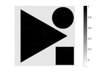
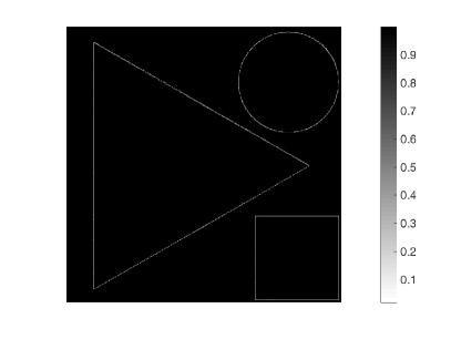
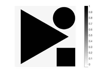
Figure 2: Example 1 ($\sigma=0.1$). Top row (from left to right): original and noisy images, respectively. Middle row: $u_{\rm tv}$ (left) from Step 1 in Algorithm 1 and the corresponding $s$ (right) from Step 3. Bottom row: reconstruction using total variation with optimized $\zeta>0$ (left) and our approach (right), respectively.

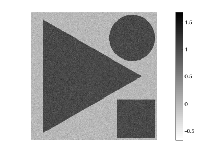
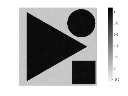
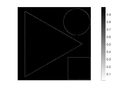
Figure 3: Example 1 ($\sigma=0.15$). Top row (from left to right): original and noisy images, respectively. Middle row: $u_{\rm tv}$ (left) from Step 1 in Algorithm 1 and the corresponding $s$ (right) from Step 3. Bottom row: reconstruction using total variation with optimized $\zeta>0$ (left) and our approach (right), respectively.

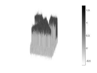
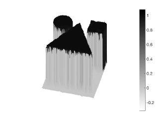
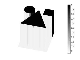
Figure 4: Example 1 ($\sigma=0.15$). Left panel: noisy image. Middle panel: reconstruction using Total Variation (TV) approach with optimal $\zeta>0$. Right panel: reconstruction using the our approach. TV tends to smooth out the edges and corners that are not aligned with the grid. On the other hand it is possible to have perfect recovery using our approach.

5.2 Example 2: stripes

In our second example we consider 6 stripes with intensities equal to 0.8, 0.7, 0.6, 0.5, 0.4 and 0.35 (from left to right), respectively (cf. Figure 5 (top row left)). As in the previous example we again consider two additive noise levels with mean 0 standard deviations $0.1$ and $0.15$ respectively. Our results are shown in Figures 5 and 6 respectively. Here again we first find $S$ by using Algorithm 1 using the parameters $\zeta=0.2$, ${\rm tol}_{\rm tv}=10e$-4, $N_{\rm refine}=8$, $\lambda=15$, $\beta=0.99$, $\nu=100$. We further set $\mu=2900$ in (4.2). We then solve for $V$. We call $\mathrm{tr}_{\Omega}\>V$ as our reconstruction. A comparison between PSNR and SSIM is shown in Table 2. As we noticed in the previous example we again obtain visually almost perfect reconstruction using our approach.

$\sigma$	PSNR (TV)	PSNR (New)	SSIM (TV)	SSIM (New)
0.1	3.6253e+01	2.7917e+01	9.0799e-01	9.4789e-01
0.15	3.3616e+01	2.7419e+01	8.7028-01	9.3000e-01

Table 2: Example 2: PSNR and SSIM using two different standard deviations ($\sigma=0.1$ and $\sigma=0.15$) using TV and proposed scheme (New).

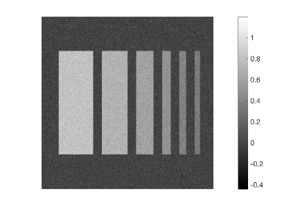
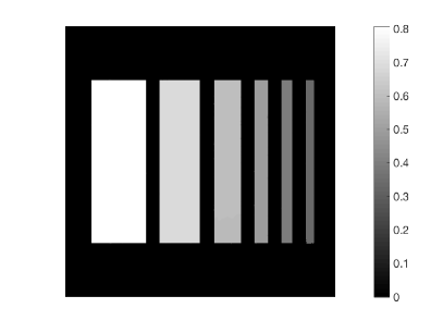
Figure 5: Example 2 ($\sigma=0.1$). Top row (from left to right): original and noisy images, respectively. Middle row: $u_{\rm tv}$ (left) from Step 1 in Algorithm 1 and the corresponding $s$ (right) from Step 3. Bottom row: reconstruction using total variation with optimized $\zeta>0$ (left) and our approach (right), respectively.

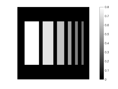
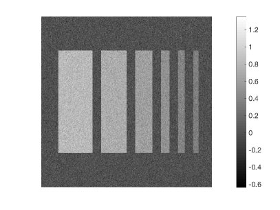
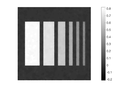
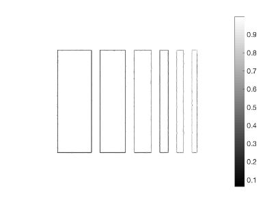
Figure 6: Example 2 ($\sigma=0.15$). Top row (from left to right): original and noisy images, respectively. Middle row: $u_{\rm tv}$ (left) from Step 1 in Algorithm 1 and the corresponding $s$ (right) from Step 3. Bottom row: reconstruction using total variation with optimized $\zeta>0$ (left) and our approach (right), respectively.

5.3 Example 3: cameraman

In the first two examples we considered synthetic images. In our final example we consider a more realistic situation. We consider a prototypical image of the cameraman (cf. Figure 7). As in the previous examples we again consider two additive noise levels with standard deviations $0.1$ and $0.15$ respectively. Our results are shown in Figures 7 and 8, respectively

At first we apply the Algorithm 1 to find $S$. Here we have set the underlying parameters as $\zeta=0.2$, ${\rm tol}_{\rm tv}=10e$-4, $N_{\rm refine}=8$, $\lambda=0.7$, $\beta=0.99$, $\nu=20$. We further set $\mu=10^{4}$ in (4.2). We then solve for $V$ and we call $\mathrm{tr}_{\Omega}\>V$ as our reconstruction. A comparison between PSNR and SSIM is shown in Table 3. As we noticed in the previous examples we again obtain better reconstructions using our approach.

6 Conclusion and further directions

A new variational model associated to the fractional Laplacian was introduced. In particular, we have identified a weighted Sobolev space with respect to the weight $w=y^{1-2s(x)}$ appropriate for the treatment of the problem. We have shown that in general these weights are not of Muckenhoupt type, and have established that the trace space embeds in an $s-$weighted Lebesgue space. We have provided a discretization method for the full problem, and an algorithm for its resolution that also builds a selection procedure for $s$. The full scheme is advantageous when it comes to recovery of discontinuous features, details, homogeneous regions, and also for contrast preservation, in data perturbed by additive noise.

Future research directions are multiple, we enumerate some of them.

1) The study of the optimization problem (3.1), seems to be the first step for the identification of a possible definition for $(-\Delta)^{s(x)}$. Such a task does not seem directly approachable via spectral or functional calculus points of view.

2) Full characterization of the trace space for $H$ and $H_{0}$. We have identified the embedding of $\mathrm{tr}_{\Omega}\>H$ into $L^{2}(\Omega;s(x)^{2})$, but it would be of interest to understand the Sobolev regularity of $\mathrm{tr}_{\Omega}\>H$.

3) Differentiability and stability properties of the solution to (3.1) with respect to $s$. For the optimal selection of $s$, it is required to identify a topology over an admissible set for $s$, so that solutions to (3.1), are stable with respect to perturbations. This seems like a complex task where the usual obstacles from homogenization and convergence of differential operators are present. In addition, difficulty is increased as the solutions to (3.1) belong to a state space depending on $s$ as well. The differentiability issue is further more complex, but such a study will be the first step in establishing stationarity systems useful for implementation in the optimal selection of $s$.

4) The extension of the presented methods to a general class of inverse problems. Problem (3.1), admits the following generalization

$$\min_{u\in H(\mathcal{C};y^{1-2s(x)})}\int_{\mathcal{C}}y^{1-2s(x)}\left(\theta|u|^{2}+|\nabla u|^{2}\right)\>\mathrm{d}x\>\mathrm{d}y+\frac{\mu}{2}\int_{\Omega}s(x)^{2}|K(\mathrm{tr}_{\Omega}\>u)-f|^{2}\>\mathrm{d}x,$$

where $K$ is a bounded linear operator on $L^{2}(\Omega;s(x)^{2})$. This would allow to deal with the problem of finding $y$ such that $Ky=f$. In this case, the choice of $s$ could be simply associated with regions of the domain $\Omega$ where it is more important to recover $y$ more accurately.

$\sigma$	PSNR (TV)	PSNR (New)	SSIM (TV)	SSIM (New)
0.1	2.7054e+01	2.9640e+01	8.0475e-01	8.3653e-01
0.15	2.4376e+01	2.6884e+01	7.4340e-01	7.9335e-01

Table 3: Example 3:PSNR and SSIM using two different standard deviations ($\sigma=0.1$ and $\sigma=0.15$) using TV and proposed scheme (New).

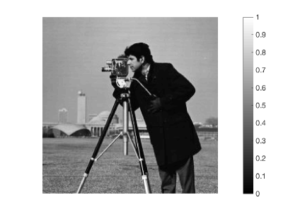
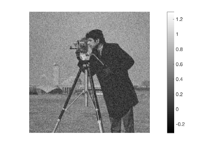
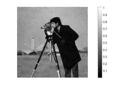
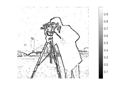
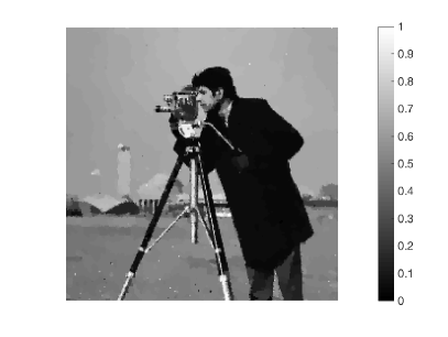
Figure 7: Example 3 ($\sigma=0.1$). Top row (from left to right): original and noisy images, respectively. Middle row: $u_{\rm tv}$ (left) from Step 1 in Algorithm 1 and the corresponding $s$ (right) from Step 3. Bottom row: reconstruction using total variation with optimized $\zeta>0$ (left) and our approach (right), respectively.

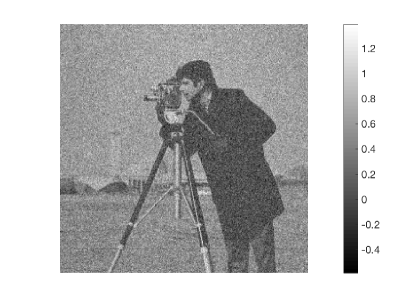
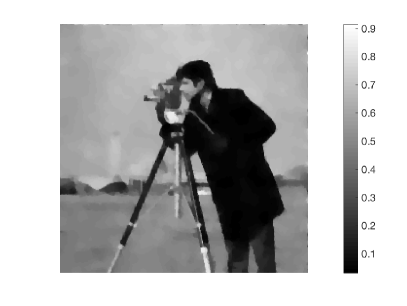
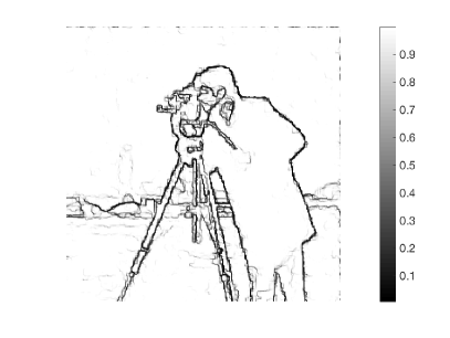
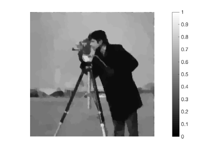
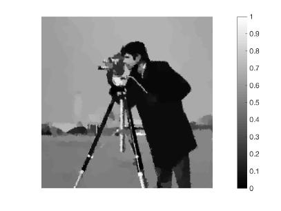
Figure 8: Example 3 ($\sigma=0.15$). Top row (from left to right): original and noisy images, respectively. Middle row: $u_{\rm tv}$ (left) from Step 1 in Algorithm 1 and the corresponding $s$ (right) from Step 3. Bottom row: reconstruction using total variation with optimized $\zeta>0$ (left) and our approach (right), respectively.

References

- [1] H. Antil and S. Bartels. Spectral Approximation of Fractional PDEs in Image Processing and Phase Field Modeling. Comput. Methods Appl. Math., 17(4):661–678, 2017.
- [2] H. Antil, J. Pfefferer, and S. Rogovs. Fractional operators with inhomogeneous boundary conditions: Analysis, control, and discretization. arXiv preprint arXiv:1703.05256, 2017.
- [3] H. Antil and C.N. Rautenberg. Fractional elliptic quasi-variational inequalities: theory and numerics. Accepted in Interfaces and Free Boundaries. Available in https://arxiv.org/pdf/1712.07001.pdf, 2018.
- [4] H. Attouch, G. Buttazzo, and G. Michaille. Variational analysis in Sobolev and BV spaces, volume 17 of MOS-SIAM Series on Optimization. Society for Industrial and Applied Mathematics (SIAM), Philadelphia, PA; Mathematical Optimization Society, Philadelphia, PA, second edition, 2014. Applications to PDEs and optimization.
- [5] L. Caffarelli and L. Silvestre. An extension problem related to the fractional Laplacian. Comm. Part. Diff. Eqs., 32(7-9):1245–1260, 2007.
- [6] L.A. Caffarelli and P.R. Stinga. Fractional elliptic equations, Caccioppoli estimates and regularity. Ann. Inst. H. Poincaré Anal. Non Linéaire, 33(3):767–807, 2016.
- [7] A. Capella, J. Dávila, L. Dupaigne, and Y. Sire. Regularity of radial extremal solutions for some non-local semilinear equations. Comm. Part. Diff. Eqs., 36(8):1353–1384, 2011.
- [8] A. Chambolle. An algorithm for total variation minimization and applications. J. Math. Imaging Vision, 20(1-2):89–97, 2004. Special issue on mathematics and image analysis.
- [9] W. Dörfler. A convergent adaptive algorithm for Poisson’s equation. SIAM J. Numer. Anal., 33(3):1106–1124, 1996.
- [10] J. Duoandikoetxea. Fourier analysis, volume 29 of Graduate Studies in Mathematics. American Mathematical Society, Providence, RI, 2001.
- [11] V. Gol’dshtein and A. Ukhlov. Weighted Sobolev spaces and embedding theorems. Trans. Amer. Math. Soc., 361(7):3829–3850, 2009.
- [12] P.C. Hansen and D.P. O’Leary. The use of the -curve in the regularization of discrete ill-posed problems. SIAM J. Sci. Comput., 14(6):1487–1503, 1993.
- [13] M. Hintermüller and C.N. Rautenberg. Optimal selection of the regularization function in a weighted total variation model. Part I: Modelling and theory. J. Math. Imaging Vision, 59(3):498–514, 2017.
- [14] M. Hintermüller, C.N. Rautenberg, T. Wu, and A. Langer. Optimal selection of the regularization function in a weighted total variation model. Part II: Algorithm, its analysis and numerical tests. J. Math. Imaging Vision, 59(3):515–533, 2017.
- [15] A. Kufner. Weighted Sobolev spaces. A Wiley-Interscience Publication. John Wiley & Sons, Inc., New York, 1985. Translated from the Czech.
- [16] A. Kufner and B. Opic. How to define reasonably weighted Sobolev spaces. Comment. Math. Univ. Carolin., 25(3):537–554, 1984.
- [17] A. Kufner and A.-M. Sändig. Some applications of weighted Sobolev spaces, volume 100 of Teubner-Texte zur Mathematik [Teubner Texts in Mathematics]. BSB B. G. Teubner Verlagsgesellschaft, Leipzig, 1987. With German, French and Russian summaries.
- [18] J.L. Lions. Théorèmes de trace et d’interpolation. Annali della Scuola Normale Superiore di Pisa-Classe di Scienze, 13(4):389–403, 1959.
- [19] D. Meidner, J. Pfefferer, K. Schürholz, and B. Vexler. -finite elements for fractional diffusion. arXiv preprint arXiv:1706.04066, 2017.
- [20] A. Nekvinda. Characterization of traces of the weighted Sobolev space on . Czechoslovak Math. J., 43(118)(4):695–711, 1993.
- [21] R.H. Nochetto, E. Otárola, and A.J. Salgado. A PDE approach to fractional diffusion in general domains: A priori error analysis. Found. Comput. Math., 15(3):733–791, 2015.
- [22] R.H. Nochetto, K.G. Siebert, and A. Veeser. Theory of adaptive finite element methods: an introduction. In Multiscale, nonlinear and adaptive approximation, pages 409–542. Springer, Berlin, 2009.
- [23] L.I. Rudin, S. Osher, and E. Fatemi. Nonlinear total variation based noise removal algorithms. Phys. D, 60(1-4):259–268, 1992. Experimental mathematics: computational issues in nonlinear science (Los Alamos, NM, 1991).
- [24] P.R. Stinga and J.L. Torrea. Extension problem and Harnack’s inequality for some fractional operators. Comm. Part. Diff. Eqs., 35(11):2092–2122, 2010.
- [25] B.O. Turesson. Nonlinear potential theory and weighted Sobolev spaces. Springer, 2000.
- [26] Z. Wang, A.C. Bovik, H.R. Sheikh, and E.P. Simoncelli. Image quality assessment: from error visibility to structural similarity. IEEE transactions on image processing, 13(4):600–612, 2004.
- [27] V. V. Zhikov. On weighted Sobolev spaces. Mat. Sb., 189(8):27–58, 1998.
- [28] V. V. Zhikov. On the density of smooth functions in a weighted Sobolev space. Dokl. Akad. Nauk, 453(3):247–251, 2013.