Theoretical uncertainties of the elastic nucleon-deuteron scattering observables

Abstract

Theoretical uncertainties of various types are discussed for the nucleon-deuteron elastic scattering observables at the incoming nucleon laboratory energies up to 200 MeV. We are especially interested in the statistical errors arising from uncertainties of parameters of a nucleon-nucleon interaction. The obtained uncertainties of the differential cross section and numerous scattering observables are in general small, grow with the reaction energy and amount up to a few percent at 200 MeV. We compare these uncertainties with the other types of theoretical errors like truncation errors, numerical uncertainties and uncertainties arising from using the various models of nuclear interaction. We find the latter ones to be dominant source of uncertainties of modern predictions for the three-nucleon scattering observables. To perform above mentioned studies we use the One-Pion-Exchange Gaussian potential derived by the Granada group, for which the covariance matrix of its parameters is known, and solve the Faddeev equation for the nucleon-deuteron elastic scattering. Thus beside studying theoretical uncertainties we also show a description of the nucleon-deuteron elastic scattering data by the One-Pion-Exchange Gaussian model and compare it with results obtained with other nucleon-nucleon potentials, including chiral N⁴LO forces from the Bochum-Bonn and Moscow(Idaho)-Salamanca groups. In this way we confirm the usefulness and high quality of the One-Pion-Exchange Gaussian force.

I Introduction

One of the main goals of nuclear physics is to establish properties of the nuclear interactions. After many years of investigations we are now in position to study details of the nuclear forces both from the theoretical as well as the experimental sides. It has been found that the three-nucleon (3$N$) system, which allows to probe also the off-energy-shell properties of the nuclear potential, is especially important for such studies. Moreover, to obtain a precise description of the 3$N$ data one has to supplement the two-nucleon (2$N$) interaction by a 3$N$ force acting in this system. Currently the structure of 3$N$ force is still unclear and many efforts are directed to fix 3$N$ force properties. However, in order to obtain trustable and precise information from a comparison of 3$N$ data with predictions based on theoretical models it is necessary to take into account, or at least to estimate, in addition to the uncertainties of data also the errors of theoretical predictions.

The precision of the experimental data has significantly increased and achieved in recent measurements a high level, see e.g. Refs. Sekiguchi ; Weisel ; Przewoski ; Kistryn ; Howell for examples of state-of-the-art experimental studies in the three-nucleon sector. Precision of these and other experiments has become so high that the question about the uncertainties of the theoretical predictions is very timely PRA_Editors_remark . In the past the theoretical uncertainties for observables in three-nucleon reactions were estimated by comparing predictions based on various models of nuclear interactions Witala2001 or by performing benchmark calculations using the same interaction but various theoretical approaches benchmarks ; COR90 ; HUB95 ; FRI90b ; FRI95 . Such a strategy was dictated by a) a common belief that a poor knowledge about the nuclear forces, reflected by the existence of very different models of nuclear interaction, is a dominant source of the theoretical uncertainty, b) lack of knowledge about the correlations between nucleon-nucleon ($NN$) potential parameters, c) using inconsistent models of 2$N$ and 3$N$ forces, and last but not least d) a magnitude of uncertainties of experimental data available at the time. Nowadays these arguments, at least partially, are no longer valid due to the above mentioned progress in experimental techniques, progress in the derivation of consistent 2$N$ and 3$N$ interactions, e.g. within the Chiral Effective Field Theory ($\chi$EFT)  Epelbaum_review ; Bernard1 ; Bernard2 ; Machleidt-review ; Machleidt2017 and due to availability of new models of nuclear forces, where free parameters are fixing by performing a careful statistical analysis Navarro_Corase ; Navarro_OPE . As a consequence, the estimation of theoretical uncertainties has become again an important issue in theoretical studies.

An extensive introduction to an error estimation for theoretical models was given in Ref. Dobaczewski , followed by a special issue of J. Phys. G: Nucl. Part. Phys. SpecialIssue . In the latter reference many applications of the error estimation to nuclear systems and processes are discussed. However, omitting the few-nucleon reactions, the authors focus mainly on models used in direct fitting to data or on models used in nuclear structure studies. Among the other papers focused on the estimation of theoretical uncertainties of $NN$ interaction we refer the reader to works by A.Ekström et al. Ekstrom , R.Navarro Pérez et al. Navarro_OPE ; Navarro_TPE ; Navarro-review and to a recent work by P.Reinert et al. Reinert . Simultaneously, the Bayesian approach to estimate uncertainties in the 2$N$ system was derived in Ref. Furnstahl with some applications shown again in Ref. SpecialIssue . Beyond the 2$N$ system, the uncertainty of theoretical models has been recently studied in the context of nuclear structure calculations for which such an evaluation is important also from a practical point of view. Namely, predictions for many-nucleon systems require not only a huge amount of advanced computations but also rely, e.g. in the case of the No-Core shell model NCSM , on extrapolations to large model spaces. A knowledge of precision of the theoretical models is important for efficient use of available computer resources.

Studies of theoretical uncertainties in few-nucleon reactions are less advanced. Beside the above mentioned attempts to estimate their magnitudes by means of benchmark calculations most efforts in the field were orientated to estimate uncertainties present in the $\chi$EFT approach Epelbaum-review . In this case three sources of theoretical uncertainties have been investigated: the truncation of the chiral expansion at a finite order (what results in the so-called truncation errors), the introduction of regulator functions (what results in a cut-off dependence), and the procedure of fixing values of low-energy constants. A simple prescription how to estimate the truncation errors was proposed by E.Epelbaum and collaborators for the 2$N$ system imp1 and adopted also for 3$N$ systems, for the case where predictions were based on a two-body interaction Binder only. It was found that both for pure nuclear systems Binder , as well as for electroweak processes Skibinski_electroweak the magnitude of truncation errors strongly decreases with the order of chiral expansion and at the fifth order (N⁴LO) it becomes relatively small. The prescription of Ref. imp1 is in agreement with the Bayesian approach Furnstahl , see also the recent work Melendez for a discussion of the Bayesian truncation errors for the $NN$ observables. The dependence of the chiral predictions on used regulator functions and their parameters has been studied since the first applications of chiral potentials to the 2$N$ and 3$N$ systems Epelbaum_start ; Epelbaum_3N ; Machleidt_force . The regulator dependence of chiral forces was broadly discussed in the past, see e.g. Machleidt_regul and various regulator functions were proposed. The non-local regularization in the momentum space was initially used and estimations of the theoretical uncertainties of the 2$N$ and many-body observables related to regulators were made by comparing predictions obtained with various values of regularization parameters. It was found that the non-local regularization leads to an unwanted dependence of observables on the parameters used. This dependence was especially strong for predictions for the nucleon-deuteron ($Nd$) elastic scattering based on 2$N$ and 3$N$ forces at the next-to-next-to-next-to leading order (N³LO) of chiral expansion Witala_lenpic1 and for the electromagnetic processes in the 3$N$ systems when also the leading meson-exchange currents were taken into account Rozpedzik ; Skibinski_chiral_elmag_mec . These results were one of the reasons for introducing another, the so-called ”semi-local” method of regularization of chiral forces. Such an improved method was presented and applied to the $NN$ system in Refs. imp1 ; imp2 , leading to weak cut-off dependence of predictions in two-body system at chiral orders above the leading order. Similar picture of weak dependence of predictions based on the chiral forces of Refs. imp1 ; imp2 was found for $Nd$ elastic scattering Binder and for various electroweak processes Skibinski_electroweak . Also the nuclear structure calculations confirmed this observation improved_in_structure ; lenpic_long_paper .

The estimation of the theoretical uncertainties arising from an uncertainty of the potential parameters (which we will call in the following also a statistical error) has not been studied yet, to the best of our knowledge, in $Nd$ scattering. Within this paper we investigate how such statistical uncertainties propagate from the $NN$ potential parameters to the $Nd$ scattering observables. We also compare them with the remaining theoretical uncertainties for the same observables. To this end we use, for the first time in $Nd$ scattering, the One-Pion-Exchange (OPE) Gaussian $NN$ interaction derived recently by the Granada group Navarro_OPE . The knowledge of the covariance matrix of the OPE-Gaussian potential parameters is a distinguishing feature of this interaction. This is also crucial for our investigations as we use a statistical approach to estimate theoretical uncertainties. Namely, given the covariance matrix for the potential parameters, we sample 50 sets of the potential parameters and, after calculating for each set the 3$N$ observables, we study statistical properties of the obtained predictions. The OPE-Gaussian interaction is described briefly in Sec. II and our method to obtain statistical errors is discussed step by step in Sec. III. The OPE-Gaussian force has been already used, within the same method, to estimate the statistical uncertainty of the ³H binding energy Perez_CONF which was found to be around 15 keV ($\approx 0.16\%$).

The paper is organized as follows: in Sec. II we show the essential elements of our formalism, describe its numerical realization and give some more information on the OPE-Gaussian potential and the chiral models used. In Sec. III we present predictions for the $Nd$ elastic scattering observables obtained with the OPE-Gaussian force and compare them with predictions based on the AV18 $NN$ potential AV18 . We also discuss various estimators of uncertainties in hand for the 3$N$ scattering observables. In Sec. IV we compare, for a few chosen observables, the theoretical uncertainties arising from various sources, including the truncation errors and the regulator dependence. Here, beside the OPE-Gaussian potential and other semi-phenomenological $NN$ forces, we also use the chiral interaction of Ref. imp1 ; imp2 and, for the first time in the $Nd$ scattering, the chiral N⁴LO interaction recently derived by the Moscow(Idaho)-Salamanca group Machleidt2017 . Finally, we summarize in Sec. V.

II Formalism

The formalism of the momentum space Faddeev equation is one of the standard techniques to investigate 3$N$ reactions and has been described in detail many times, see e.g. Glockle-raport ; Glockle-book . Thus we only briefly remind the reader of its key elements.

For a given $NN$ interaction $V$ we solve the Lippmann-Schwinger equation $t=V+V\tilde{G_{0}}t$ to obtain matrix elements of the 2$N$ $t$ operator, with $\tilde{G_{0}}$ being the 2$N$ free propagator. These matrix elements enter the 3$N$ Faddeev scattering equation which, neglecting the 3$N$ force, takes the following form

$$T|\phi\rangle=tP|\phi\rangle+tPG_{0}T|\phi\rangle.$$ (1)

The initial state $|\phi\rangle$ is composed of a deuteron and a momentum eigenstate of the projectile nucleon, $G_{0}$ is the free 3$N$ propagator and $P$ is a permutation operator.

The transition amplitude for the elastic $Nd$ scattering process $\langle\phi^{\prime}|U|\phi\rangle$ contains the final channel state $|\phi^{\prime}\rangle$ and is obtained as

$$\langle\phi^{\prime}|U|\phi\rangle=\langle\phi^{\prime}|PG_{0}^{-1}|\phi\rangle+\langle\phi^{\prime}|PT|\phi\rangle\;,$$ (2)

from which observables can be obtained in the standard way Glockle-raport .

Equation (1) is solved in the partial wave basis comprising all 3$N$ states with the two-body subsystem total angular momentum $j\leq 5$ and the total 3$N$ angular momentum $J\leq\frac{25}{2}$.

Since we obtained the bulk of our results with the OPE-Gaussian interaction Navarro_OPE , we briefly remind now the reader of a structure of this potential. A basic concept at the heart of this force is analogous to the one stated behind the well-known AV18 interaction AV18 . The OPE-Gaussian potential $V(\vec{r})$ is composed of the long-range $V_{long}(\vec{r})$ and the short-range $V_{short}(\vec{r})$ parts

$$V(\vec{r})=V_{short}(\vec{r})\theta(r_{c}-r)+V_{long}(\vec{r})\theta(r-r_{c}),$$ (3)

where $r_{c}$=3 fm and the $V_{long}(\vec{r})$ part contains the OPE force and the electromagnetic corrections. The $V_{short}(\vec{r})$ component is built from 18 operators $\hat{O}_{n}$, among which 16 are the same as in the AV18 model. Each of them is multiplied by a linear combination of the Gaussian functions $F_{k}(r)=\exp{(-r^{2}/(2a_{k}^{2}))}$, with $a_{k}=\frac{a}{1+k}$, and the strength coefficients $V_{k,n}$:

$$V_{short}(\vec{r})=\sum\limits_{n=1}^{18}\hat{O}_{n}\left[\sum\limits_{k=1}^{4}V_{k,n}F_{k}(r)\right].$$ (4)

The free parameter $a$ present in the $F_{k}(r)$ functions together with the parameters $V_{k,n}$ have been fixed from the data. It is worth noting that to this end the ”3$\sigma$ self-consistent database” Navarro_Corase was used. It incorporates 6713 proton-proton and neutron-proton data, gathered within the years 1950 to 2013, in the laboratory energy range $E_{lab}$ up to 350 MeV. The careful statistical revision of data and the fitting procedure allowed the authors of Ref. Navarro_OPE to confirm good statistical properties of their $\chi^{2}$ fit, e.g. by checking the normality of residuals. The $\chi^{2}/data$ for the OPE-Gaussian force is 1.06 as fitted to data enumerated in Ref. Navarro_Corase . We have been equipped by the authors of Ref. Navarro_OPE with 50 sets of parameters $\{V_{k,n},a\}$ obtained by a correlated sampling from the multivariate normal distribution with a known covariance matrix (see Navarro_sampling for details). The OPE-Gaussian model, as having a similar structure to the AV18 force, but being fitted to the newer data can be regarded as a refreshed version of the standard AV18 model. In the $NN$ sector these two potentials lead to a slightly different description of phase shifts, especially at energies above 150 MeV in the ${}^{3}F_{2}$ and ${}^{3}D_{3}$ partial waves Navarro_OPE . Thus it seems to be interesting to compare predictions for $Nd$ scattering given by both potentials.

Beside the OPE-Gaussian and the AV18 models we show in Sec. IV predictions based on two chiral forces at N⁴LO, derived by R.Machleidt and collaborators Machleidt2017 and by E.Epelbaum and collaborators imp1 ; imp2 . In the case of the first of these forces the non-local regularization, applied directly in momentum space, has been used. The regulator function is taken as $f(p^{\prime},p)=\exp{(\,\rm{-}\,(\frac{p^{\prime}}{\Lambda})^{2n}\,\rm{-}\,(\frac{p}{\Lambda})^{2n})}$, where $n$ depends on regarded operators (e.g. $n=4$ for the one-pion exchange potential). Three values of the cutoff parameter $\Lambda$ (450, 500 and 550 MeV) were suggested for this potential and are also used in this paper. In the case of the N⁴LO potential and $\Lambda=500$ MeV the $\chi^{2}/{\rm data}=1.15$ for the combined neutron-proton and proton-proton data in the energy range 0-290 MeV Machleidt2017 . In this paper we show for the first time the predictions of this new chiral potential at N⁴LO for the $Nd$ elastic scattering observables. As mentioned above, in the approach of Refs. imp1 ; imp2 the semi-local regularization of nuclear forces is performed in coordinate space with the regulator function $f(r)=[1-\exp{(\,\rm{-}\,(\frac{r}{R})^{2})}]^{6}$, where $r$ is the distance between nucleons and $R$ is the regulator parameter. The authors of Ref. imp1 suggested five values of the regulator $R=$0.8, 0.9, 1.0, 1.1, and 1.2 fm. The best description of the $NN$ observables is achieved with $R$=0.9 fm and $R$=1.0 fm, and leads to the $\chi^{2}/{\rm data}\approx 1.14$ at $R$=0.9 fm for the N⁴LO force Reinert when using the “3$\sigma$-self-consistent database” from Ref. Navarro_Corase . This value is comparable with the ones obtained for the semi-phenomenological potentials.

III The OPE-Gaussian predictions for Nd scattering and their statistical errors

III.1 Determination of statistical uncertainty in 3N system

To determine the theoretical uncertainty arising from the 2$N$ potential parameters we took the following steps:

1. We prepared various sets of the potential parameters.

   Actually, this step had been already taken by the Granada group as a part of their study of the statistical uncertainty of the ³H binding energy. They provided us with fifty sets ($S_{i}$ with $i=1,\dots,50$) of 42 potential parameters (drawn from the multivariate normal distribution with known expectation values and covariance matrix) and one set of expectation values of potential parameters ($S_{0}$). Such a relatively big sample of fifty-one sets allows us to obtain statistically meaningful conclusions.

2. For each set $S_{i}$ ($i=0,1,\dots,50$) we calculated the deuteron wave function and the $t$ matrix, solved, at each considered energy, the Faddeev equation (1), calculated the scattering amplitude (Eq. (2)) and finally computed observables. As a result the angular dependence of various scattering observables is known for each set of parameters $S_{i}$.

The predictions obtained in such a way allow us to study:

1. for a given energy $E$, an observable $O$, and a scattering angle $\theta$, the empirical probability density function of the observable $O(E,\theta)$ resulting when various sets $S_{i},(i=1,\dots,50)$ are used;

2. for a given observable $O$, both the angular and energy dependencies of results based on various sets $S_{i}$.

Based on these studies we can conclude on the measure of statistical uncertainties and quality of elastic $Nd$ scattering data description. This is a content of the next two subsections.

III.2 Measure of statistical uncertainty

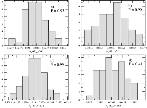
Figure 2: The histograms and the P-values for the Shapiro-Wilk test for the nucleon analyzing power A_y in $Nd$ elastic scattering at the incoming nucleon laboratory energy $E$=13 MeV and the scattering angle: a) $\theta_{\rm{c.m.}}=30^{\circ}$, b) $\theta_{\rm{c.m.}}=75^{\circ}$, c) $\theta_{\rm{c.m.}}=120^{\circ}$, and d) $\theta_{\rm{c.m.}}=165^{\circ}$, obtained with 50 sets of the OPE-Gaussian potential parameters.

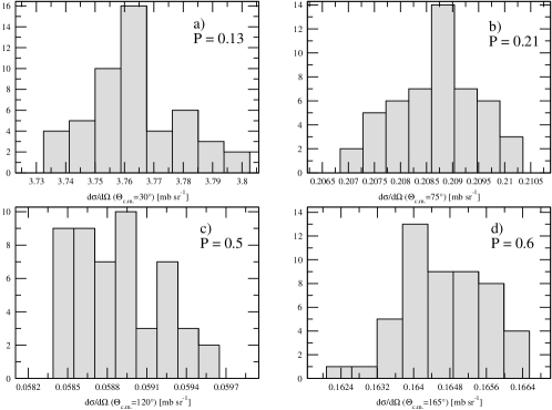
Figure 3: The same as in Fig. 1 but at $E$=200 MeV.

Our first task is to choose an estimator of the theoretical uncertainties in question. Due to a big complexity of calculations required to obtain the 3$N$ scattering observables we are not able a priori to determine analytically the probability distribution function of the resulting 3$N$ predictions and consequently to choose the best estimator to describe the dispersion of results. In Figs. 1 and 2 we show the empirical distributions (histograms) of the cross section $d\sigma/d\Omega$ and the nucleon analyzing power A_y at the nucleon laboratory energy $E$=13 MeV and at four c.m. scattering angles: $\theta_{\rm{c.m.}}$ = 30^∘, 75 ^∘, 120^∘ and 165^∘. The same observables at the same $\theta_{\rm{c.m.}}$ angles but at $E$=200 MeV are shown in Figs. 3 and 4, respectively. It is clear that the distribution of the predictions cannot be regarded as the normal distribution. To obtain quantitative information on the distribution we have performed the Shapiro-Wilk test Shapiro-Wilk-Test , which belongs to the strongest statistical tests of normality. As is seen from the obtained P-values (the smaller P-value the more unlikely the predictions are normally distributed) given in Figs. 1-4, in many cases the resulting distributions of the cross section and the nucleon analyzing power cannot be regarded with high confidence as normal distributions. This restricts a choice of the dispersion estimators - neither the commonly used confidence interval nor the usual estimators for the standard deviation can be used directly as they are tailored to the normal distribution. Thus we considered the following estimators for the statistical error of the observable $O(E,\theta)$ (at a given energy and a scattering angle):

1. $\frac{1}{2}\Delta_{100\%}\equiv\frac{1}{2}(max_{i}(O_{i})-min_{i}(O_{i})\,)$, where the minimum and maximum are taken over all predictions based on different sets of the $NN$ potential parameters $S_{i}$, $i=1,2,\dots,50$;

2. $\frac{1}{2}\Delta_{68\%}\equiv\frac{1}{2}(max_{i}(O_{i})-min_{i}(O_{i})\,)$, where the minimum and maximum are taken over 34 (68% of 50) predictions based on different sets of the $NN$ potential parameters; The set of 34 observables is constructed by disposing of the 8 smallest and the 8 biggest predictions for the observable $O(E,\theta)$;

3. $\frac{1}{2}$IQR – the half of standard estimator of the interquartile range being the difference between the third and the first quartile $IQR=Q_{3}-Q_{1}$. For the sample of size 50 this corresponds to taking the half of difference between the predictions on 37th and 13th position in a sample sorted in the ascending order. The flexibility in applying this measure to the non-normal distribution is a great asset to the IQR;

4. $\sigma(O)$ – the sample standard deviation $\sigma(O)=\sqrt{\frac{1}{n-1}\sum_{i=1}^{n}(x_{i}-\bar{x})^{2}}$, where $\bar{x}$ is the usual mean value. The disadvantage of this estimator is that on formal grounds it cannot be applied to samples from an arbitrary probability distribution.

The $\frac{1}{2}\Delta_{100\%}$ and the $\sigma(O)$ are sensitive to the possible outliers in the sample and thus taking them as estimators of dispersion can lead to overestimation of the statistical error. On the other hand the IQR is calculated using only half of the elements in the sample and thus can lead to underestimation of the theoretical uncertainty. Thus we decided to adapt the $\frac{1}{2}\Delta_{68\%}$ as an optimal measure of predictions’ dispersion and consequently as an estimator of the theoretical uncertainty in question. The same choice has been made in a study of the statistical error of the ${}^{3}H$ binding energy in Ref. Navarro_sampling . The similarity to the standard deviation is one more advantage of $\frac{1}{2}\Delta_{68\%}$ since the comparison of the theoretical errors with the experimental (statistical) uncertainties, delivered usually in the form of standard deviations, is finally unavoidable.

However, in Tab. 1 we compare values of the above mentioned estimators for the $Nd$ elastic scattering differential cross section at three energies of the incoming nucleon and at four c.m. scattering angles. By definition $\frac{1}{2}{\rm IQR}\leq\frac{1}{2}\Delta_{68\%}\leq\frac{1}{2}\Delta_{100\%}$ and indeed this is observed in Tab. 1. The magnitudes of the $\frac{1}{2}\Delta_{68\%}$ is very close to the measure based on the sample standard deviation $\sigma(d\sigma/d\Omega)$ and in practice it does not matter which of these estimators is used. The relative uncertainty (exemplified in the Tab. 1 for the sample standard deviation) remains below 1% for all scattering angles at $E=13$ MeV and $E=65$ MeV, and only slightly exceeds it at $E=200$ MeV. In Tab. 1 we also show values of the differential cross section obtained with the central values of the OPE-Gaussian potential parameters and mean values of predictions calculated separately for the 50 ($M_{100\%}$) or 34 ($M_{68\%}$) sets of parameters $S_{i}$. Also here in most of the cases $d\sigma/d\Omega(S_{0})\approx M_{100\%}\approx M_{68\%}$, what shows, that the predictions based on sets $S_{i}$ for $i\neq 0$ cluster around $d\sigma/d\Omega(S_{0})$ evenly. The other observables behave in a similar way.

E [MeV]	$\theta_{\rm{c.m.}}$ [deg]	d$\sigma$/d$\Omega$(S0)	$\frac{1}{2}\Delta_{100\%}$	$\frac{1}{2}\Delta_{68\%}$	$\frac{1}{2}$IQR	$\sigma(d\sigma/d\Omega)$	$M_{100\%}$	$M_{68\%}$
	30	134.9970	0.1780	0.1025	0.0635	0.0954 (0.132%)	135.0040	135.0100
13.0	75	51.3274	0.0315	0.0153	0.0110	0.0149 (0.061%)	51.3283	51.3295
	120	9.7437	0.0347	0.0181	0.0118	0.0179 (0.356%)	9.7421	9.7420
	165	103.1210	0.1085	0.0420	0.0230	0.0462 (0.105%)	103.1190	103.1190
	30	23.7000	0.1785	0.0812	0.0569	0.0824 (0.753%)	23.7137	23.7092
65.0	75	2.3630	0.0134	0.0060	0.0040	0.0057 (0.568%)	2.3630	2.3630
	120	0.7787	0.0035	0.0015	0.0011	0.0016 (0.451%)	0.7786	0.7785
	165	4.7537	0.0174	0.0076	0.0060	0.0075 (0.366%)	4.7532	4.7535
	30	3.7626	0.0351	0.0164	0.0097	0.0162 (0.325%)	3.7634	3.7625
200.0	75	0.2088	0.0018	0.0008	0.0005	0.0008 (0.839%)	0.2087	0.2087
	120	0.0585	0.0006	0.0004	0.0003	0.0003 (1.069%)	0.0589	0.0589
	165	0.1645	0.0022	0.0009	0.0007	0.0009 (1.356%)	0.1647	0.1647

Table 1: The differential cross section d$\sigma$/d$\Omega$ obtained with the expectation values of the OPE-Gaussian potential parameters (set $S_{0}$), various estimators of its dispersion (see text) and mean values taken from 50 ($M_{100\%}$) or 34 ($M_{68\%}$) predictions. In case of the sample standard deviation $\sigma(d\sigma/d\Omega)$ also the relative magnitude $\sigma(d\sigma/d\Omega)\;/\;(d\sigma/d\Omega(S_{0}))*100\%$ is shown in brackets. All predictions are given in [mb sr^-1].

Figure 1: The histograms and the P-values for the Shapiro-Wilk test for the elastic $Nd$ scattering differential cross section d$\sigma$/d$\Omega$ [mb sr^-1] at the incoming nucleon laboratory energy $E$=13 MeV and the scattering angle: a) $\theta_{\rm{c.m.}}=30^{\circ}$, b) $\theta_{\rm{c.m.}}=75^{\circ}$, c) $\theta_{\rm{c.m.}}=120^{\circ}$, and d) $\theta_{\rm{c.m.}}=165^{\circ}$, obtained with 50 sets of the OPE-Gaussian potential parameters.

Figure 4: The same as in Fig. 2 but at $E$=200 MeV.

III.3 Nucleon-deuteron elastic scattering observables from the OPE-Gaussian model

In the following we present predictions obtained with the OPE-Gaussian $NN$ interaction for various observables in the elastic neutron-deuteron scattering process at incoming nucleon laboratory energies $E=13$ MeV, 65 MeV, and 200 MeV. We will focus on the elastic scattering cross section d$\sigma$/d$\Omega$, the nucleon vector analyzing power A_y, the nucleon to nucleon spin transfer coefficients K${}_{\rm{y}}^{\rm{y^{\prime}}}$, and the spin correlation coefficients C_y,y. However, we will also give examples for other observables.

The $Nd$ cross section is shown in Fig. 5. Apart from the solid line which represents predictions based on the OPE-Gaussian force when the expectation values of its parameters (set $S_{0}$) are used, we also show the red band representing the range of predictions obtained with the same 34 sets $S_{i}$ as used to calculate $\frac{1}{2}\Delta_{68\%}$, and the blue dashed curve showing results obtained with the AV18 interaction. The nucleon-deuteron data (at the same or nearby energies) are also added for the sake of comparison. The predictions based on the OPE-Gaussian force are in agreement with the predictions based on the AV18 potential. Only small, ($\approx 3.9$% at $E$=13 MeV and $\approx$ 3.5% at $E$=200 MeV), differences are seen in the minimum of the cross section. Similarly to the AV18, the OPE-Gaussian model clearly underestimates the data at two higher energies reflecting the known fact of growing importance of a 3$N$ force WitalaPRL ; Kuros . The statistical error arising from the uncertainty of the $NN$ force parameters is in all cases very small and red bands are hardly visible in Fig. 5.

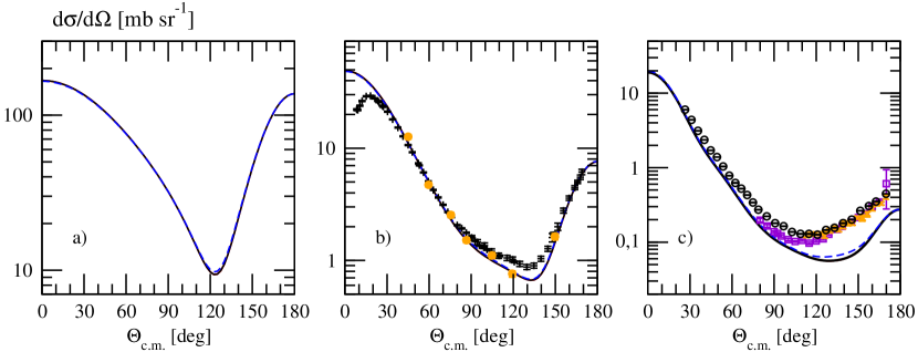
Figure 5: The $Nd$ elastic scattering cross section d$\sigma$/d$\Omega$ [mb sr^-1] at the incoming nucleon laboratory energy a) $E$=13 MeV, b) $E$=65 MeV, and c) $E$=200 MeV as a function of the c.m. scattering angle $\theta_{\rm{c.m.}}$. The black curve represents predictions obtained with the central values of the OPE-Gaussian parameters, the red band reflects statistical uncertainty discussed in this subsection, and the blue dashed curve represents predictions based on the AV18 force. The data are in b) from Ref. Shimizu ($pd$ black pluses) and Ruhl ($nd$ orange circles) and in c) from Ref. Adelberg ($pd$, $E=198$ MeV, violet squares), Ref. Igo ($pd$, $E=180$ MeV, orange x’s), and Ref. Ermisch ($pd$, $E=198$ MeV, black circles).

The OPE-Gaussian force delivers predictions which are very close to the AV18 results also for the most of the polarization observables at the energies studied here. Likewise the dispersion of predictions remains small for most of the polarization observables. Below we discuss a few of them, choosing mainly ones with the largest statistical uncertainties.

Let us start, however, with the nucleon analyzing power A_y, shown in Fig. 6. Here the uncertainties remain negligible at all energies and also the differences between predictions based on the OPE-Gaussian force and the ones obtained with the AV18 potential are tiny. Thus we see that the OPE-Gaussian model does not deliver any hint on the nature of the A_y puzzle at $E=13$ MeV.

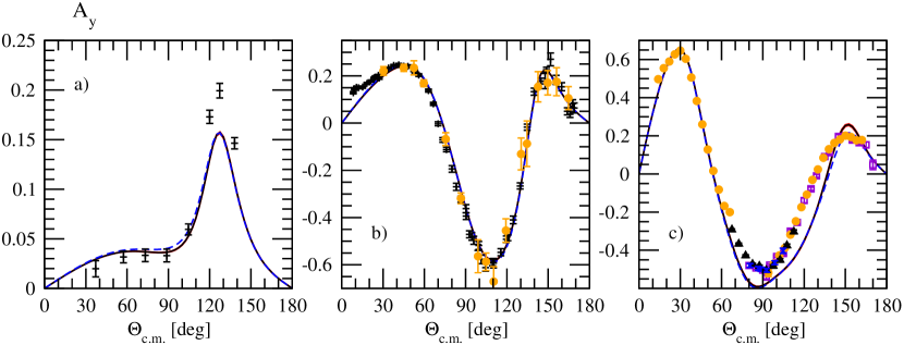
Figure 6: The nucleon analyzing power A_y for $Nd$ elastic scattering at the same energies as used in Fig. 5 as a function of the c.m. scattering angle $\theta_{\rm{c.m.}}$. Curves and band as in Fig. 5. The data in a) are from Ref. Cub-ayn13 ($nd$ black pluses), in b) are from Ref. Shimizu ($pd$ black pluses) and Ref. Ruhl ($nd$ orange circles), and in c) are from Ref. Adelberg ($pd$ violet squares), Ref. Przewoski ($pd$ $E=200$ MeV orange circles), Ref. Cadman ($pd$ $E=197$ MeV black triangles up), and Ref. Wells ($pd$ blue x’s).

We have chosen the nucleon to nucleon spin transfer coefficient K${}_{\rm{y}}^{\rm{y^{\prime}}}$ and the spin correlation coefficient C_y,y to demonstrate, in Figs. 7 and 8, respectively, changes of the statistical errors when increasing the reaction energy. For both observables dispersion of the results grows with energy, and while at lowest energy $E$=13 MeV it is negligible, at $E$=200 MeV its size is bigger, although it remains small ( $\frac{1}{2}\Delta_{68\%}<0.5\%$). In the case of C_y,y comparison with the data reveals that the spread of the OPE-Gaussian results is still smaller than uncertainties of experimental results.

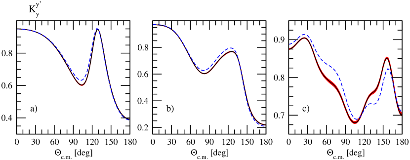
Figure 7: The nucleon to nucleon spin transfer coefficient K${}_{\rm{y}}^{\rm{y^{\prime}}}$ at the incoming nucleon laboratory energy a) $E$=13 MeV, b) $E$=65 MeV and c) $E$= 200 MeV as a function of the c.m. scattering angle $\theta_{\rm{c.m.}}$. See Fig.5 for a description of band and curves.

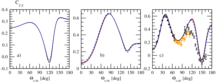
Figure 8: The spin correlation coefficient C_y,y at the incoming nucleon laboratory energy a) $E$=13 MeV, b) $E$=65 MeV and c) $E$=200 MeV as a function of the c.m. scattering angle $\theta_{\rm{c.m.}}$. See Fig.5 for a description of band and curves. In c) data are from Ref. Cadman ($pd$ $E=197$ MeV, orange circles) and Ref. Przewoski ($pd$ $E=200$ MeV, black pluses).

In Fig. 9 we show two observables for which the difference between the AV18 predictions and the OPE-Gaussian results is especially big already at the two lower energies. They are the spin correlation coefficient C_xx,y-C_yy,y at $E$=13 MeV and the deuteron to nucleon spin transfer coefficient K${}_{\rm{yz}}^{\rm{x^{\prime}}}$ at $E$=65 MeV. The difference between both predictions amounts to $\approx 19$% at the minimum of C_xx,y-C_yy,y, while the statistical error of the OPE-Gaussian results is only $\approx 2$%. For K${}_{\rm{yz}}^{\rm{x^{\prime}}}$ these differences amount to $\approx 23$% and $\approx 3$%, respectively. We see that even in these two cases the statistical uncertainty remains much smaller than uncertainty related to using various models of the $NN$ interaction.

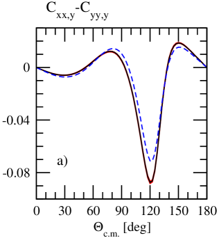
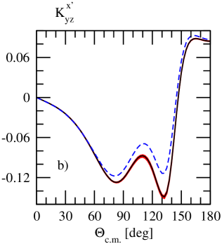
Figure 9: The spin correlation coefficient C_xx,y-C_yy,y at the incoming nucleon laboratory energy $E$=13 MeV (a) and the deuteron to nucleon spin transfer coefficient K${}_{\rm{yz}}^{\rm{x^{\prime}}}$ at the incoming nucleon laboratory energy $E$=65 MeV (b) as a function of the c.m. scattering angle $\theta_{\rm{c.m.}}$. Curves and band are as in Fig.5.

The statistical errors grow with the reaction energy. Thus in Fig. 10 we show for $E=200$ MeV a few observables with the largest uncertainties. Beside the spin transfer coefficient K${}_{\rm{y}}^{\rm{y^{\prime}}}$ already shown in Fig. 7 they are the deuteron tensor analyzing powers T₂₁ and T₂₂ and the nucleon to deuteron spin transfer coefficient K${}_{\rm{y}}^{\rm{x^{\prime}x^{\prime}}}$-K${}_{\rm{y}}^{\rm{y^{\prime}y^{\prime}}}$. While the bands representing the theoretical uncertainties are clearly visible, they still remain small compared to the experimental errors for both analyzing powers. The differences between predictions based on the AV18 potential and the OPE-Gaussian force are small. This is true also for the other Nd elastic scattering observables both at $E=200$ MeV and at the lower energies, so we conclude that the OPE-Gaussian force yields a similar description of this process compared with the AV18 potential.

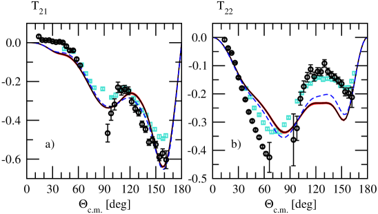
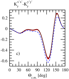
Figure 10: The deuteron tensor analyzing powers T₂₁ (a) and T₂₂ (b) and the nucleon to deuteron spin transfer coefficient K${}_{\rm{y}}^{\rm{x^{\prime}x^{\prime}}}$-K${}_{\rm{y}}^{\rm{y^{\prime}y^{\prime}}}$ (c) for $E=200$ MeV as a function of the center of mass scattering angle $\theta_{\rm{c.m.}}$. See Fig.5 for description of bands and curves. The T₂₁ and T₂₂ data are from Ref. Sekiguchi ($pd$ $E=186.6$ MeV turquoise squares) and Ref. Przewoski ($pd$ $E=200$ MeV black circles)

IV Comparison of various theoretical uncertainties in Nd scattering

It is interesting to compare the statistical error $\frac{1}{2}\Delta_{68\%}$ obtained in the previous section with the other uncertainties (like the uncertainty arising from using the various models of nuclear interaction, the uncertainty introduced by the partial wave decomposition approach, the truncation errors of chiral predictions and the uncertainties originating in the cut-off dependence of chiral forces) present in the elastic $Nd$ scattering studies and specifically in our approach.

The accuracy of predictions arising from the algorithms used in our numerical scheme, which comprises, among others, numerical integrations, interpolations and series summations, is well under control. This has been tested, e.g. by using various grids of mesh points, or more generally by benchmark calculations involving different methods to treat $Nd$ scattering COR90 ; HUB95 ; FRI90b ; FRI95 . The main contribution to theoretical uncertainties comes in our numerical realization from using a truncated set of partial waves. Typically we restrict ourselves to partial waves with the two-body total orbital momentum $j\leq 5$. Predictions for observables converge with increasing $j$, as was documented e.g. in Glockle-raport . In the following we compare the OPE-Gaussian predictions, shown in the previous section, based on all two-body channels up to $j=5$ with the predictions based on all channels up to $j=4$ only to remind the reader some facts about the convergence of our approach. However, since the differences between (not shown here) predictions based on all channels up to $j=6$ and those with $j_{max}=5$ are, based on results with other NN potentials, smaller than this for $j_{max}=5$ and $j_{max}=4$ predictions, the latter difference very likely overestimates the uncertainty arising from our computational scheme. A recent work Topolnicki compares predictions for the elastic $Nd$ scattering, based however only on the driving term of Eq. (1), obtained within the partial wave formalism with the ones from the ”three-dimensional” approach, i.e. the approach which totally avoids the partial wave decomposition and uses momentum vectors. A very good agreement between the partial waves based results and the ”three-dimensional” ones confirms that neglecting the higher partial waves in the calculations presented here practically does not affect our predictions.

Next, we would like to focus on the truncation errors and the cut-off dependence present in the chiral calculations and last but not least on the differences between predictions based on various models of the nuclear two-body interaction.

To estimate two types of theoretical uncertainties present when chiral potentials are used we calculated the elastic $Nd$ scattering observables using two $NN$ interactions at the N⁴LO: one delivered by E.Epelbaum et al. imp2 (E-K-M force) and the other derived by D.R.Entem et al. Machleidt2017 (E-M-N force). In the case of the E-K-M model the semi-local regularization with the cut-off parameter $R$ in the range between 0.8 fm and 1.2 fm is used and the breakdown scale of the $\chi$EFT is 0.4-0.6 GeV imp2 . The E-M-N model uses the chiral breaking scale of 1 GeV and the cut-off parameter $\Lambda$ for non-local regularization lies between 450 MeV and 550 MeV Machleidt2017 .

The truncation errors $\delta(O)^{(i)}$ of an observable $O$ at $i$-th order of the chiral expansion, with $i=0,2,3,\dots$, when only two-body interaction is used, can be estimated as Binder :

$$\delta(O)^{(0)} \geq max\left(Q^{2}|O^{(0)}|\,,|O^{(i\geq 0)}-O^{(j\geq 0)}|\right)\,,$$

$$\delta(O)^{(2)} = max\left(Q^{3}|O^{(0)}|\,,Q|\Delta O^{(2)}|\,,|O^{(i\geq 2)}-O^{(j\geq 2)}|\right)\,,$$

$$\delta(O)^{(i)} = max\left(Q^{i+1}|O^{(0)}|\,,Q^{i-1}|\Delta O^{(2)}|\,,Q^{i-2}|\Delta O^{(3)}|\right)\,{\rm for}\,i\geq 3\;,$$ (5)

where $Q$ denotes the chiral expansion parameter, $\Delta O^{(2)}\equiv O^{(2)}-O^{(0)}$ and $\Delta O^{(i)}\equiv O^{(i)}-O^{(i-1)}$ for $i\geq 3$. In addition conditions: $\delta(O)^{(2)}\geq Q\delta(O)^{(0)}$ and $\delta(O)^{(i)}\geq Q\delta(O)^{(i-1)}$ for $i\geq 3$ are imposed on the truncation errors $\delta(O)^{(i)}$ in case when at higher orders 3N force is not included into calculations Binder .

The uncertainty arising from the cut-off dependence can be easily quantified - we just take the difference between the minimal and the maximal prediction, separately for the E-K-M force and for the E-M-N model. However, one has to be aware that in the case of the E-K-M force the cut-off values between $R=0.9$ fm and $R=1.0$ fm are preferred in the 2$N$ system. Thus in the following we separately discuss the whole range of regulator values ($0.8$ fm $\leq R\leq 1.2$ fm) and the range restricted to $0.9$ fm $\leq R\leq 1.0$ fm only.

To estimate the uncertainty arising from using various models of nuclear forces we do not introduce any separate measure but just show the differences between predictions obtained with various interactions. Admittedly, the authors of Ref. Dobaczewski suggest in such a case to calculate the estimator of standard deviations, but it is valid only under assumptions of the same quality of all interaction models, what is not clear in the case of the presented here calculations.

The systematical review of various uncertainties for the differential cross section d$\sigma$/d$\Omega$, the nucleon analyzing power A_y, the deuteron tensor analyzing power T₂₂, and the spin correlation coefficient C_y,y is given in Figs. 11-14, respectively. In these figures, in each subplot, the predicted value of the observable is given at the bottom horizontal axis and the vertical lines are used to mark predictions based on different $NN$ forces and length of these lines has no meaning. The top horizontal axis shows the percentage relative difference $N(O)$ with respect to the OPE-Gaussian prediction and its ticks are calculated as $\tilde{x}=(\frac{x-O_{\rm{OPE-Gaussian}}}{O_{\rm{OPE-Gaussian}}})*100*sign(O_{\rm{OPE-Gaussian}})$ where $x$ are the ticks values shown at the bottom axis. In addition, for the sake of figures’ clarity, the $\tilde{x}$’s are rounded to the two digits only. Note, that the magnitude of such a relative difference depends on the magnitude of the OPE-Gaussian prediction and can increase to infinity as the OPE-Gaussian prediction approaches zero. The OPE-Gaussian results (at the central values of the parameters) are represented by vertical red lines, the AV18 ones by the black line, the CD-Bonn predictions by the blue line, the E-K-M N⁴LO $R=0.9$ fm results by the magenta solid line, the E-K-M N⁴LO $R=1.0$ fm ones by the magenta dashed line, and the E-M-N N⁴LO $\Lambda$=500 MeV ones by the green line. Horizontal lines represent magnitudes of various theoretical uncertainties and starting from the bottom they are: statistical error for the OPE-Gaussian model (the red line), difference between OPE-Gaussian predictions based on the $j_{max}=5$ and $j_{max}=4$ calculations (the orange line), regulator dependence for the E-K-M N⁴LO force in range $R$=0.8-1.2 fm (the solid magenta line), the truncation error for the E-K-M N⁴LO $R=0.9$ fm model (the dashed magenta line), regulator dependence for the E-M-N N⁴LO force in range $\Lambda$=450-550 MeV (the solid green line), and truncation error for the E-M-N N⁴LO $\Lambda$=500 MeV potential (the dashed green line). Further, subplots in various rows in Figs. 11-14 show predictions at different incoming nucleon lab. energies, which are $E=13$ MeV (top), $E=65$ MeV (middle) and $E=200$ MeV (bottom). Finally, the various columns show predictions at different scattering angles: 30^∘, 75^∘, 120^∘, and 165^∘ moving from the left to the right.

An analysis of Figs. 11-14 leads to the following conclusions:

1. In general, all models investigated here provide similar results, which differ only by a few percent at lower energies but differences between predictions grow with the increasing energy. There is no single model which gives systematically the smallest or the biggest value. There are also no two models, whose predictions for all the cases lie close to each other. Note, the above statements describe general trends but exceptions from this pattern for specific observables and angles are possible.

2. At all energies the dominant theoretical uncertainty is the one arising from using various models of the nuclear interaction.

3. The statistical errors for the OPE-Gaussian predictions are small (and with no practical importance) for all the considered observables and energies.

4. The difference between $j_{max}=5$ and $j_{max}=4$ predictions, as expected, grows with energy, however, it remains small, when compared to other uncertainties, even at $E=200$ MeV (with the only exceptions of the T₂₂ at 200 MeV and C_y,y at 65 MeV). Thus the uncertainty bound with partial wave decomposition and numerical performance is also negligible.

5. The OPE-Gaussian predictions based on the central values are always inside the range given by the statistical errors. The E-K-M results show monotonic behaviour of the predicted observables with the regulator value. In the case of the E-M-N force the middle value of regulator ($\Lambda=500$ MeV) delivers extreme (among the E-M-N ones) predictions in many cases.

6. The difference between predictions based on the two chiral N⁴LO models used (E-K-M and E-M-N) is not smaller than the difference between any other pair of predictions based on different $NN$ potentials. This suggests that there are substantial differences in the construction each of these models. Thus it seems mandatory to regard these models independently, as two different models of nuclear forces.

7. In numerous cases the two chiral approaches deliver results separated from each other by more than the estimated uncertainty for their predictions. This again points to differences between both chiral potentials (and/or to an underestimation of the corresponding total theoretical uncertainties).

8. In the case of both chiral models, the dominant uncertainty at lower energies arises from the cut-off dependence. This uncertainty is much bigger than the remaining types of errors, except for differences between various models. At higher energies the truncation errors are also important in some specific cases, e.g. the differential cross section at $\theta_{\rm{c.m.}}=120^{\circ}$ at $E=200$ MeV. In the case of A_y at $E$=200 MeV and smaller angles, the truncation errors exceed the regulator dependence for the E-K-M potential.

9. In the case of the N⁴LO E-K-M potential, the difference between predictions for $R=0.9$ fm and $R=1.0$ fm (so at the two preferred values of the regulator in the $NN$ system) is of the same size as the typical difference between any other pair of predictions, what shows strong sensitivity of the observables to the regulator parameter.

10. Comparing the cutoff dependence of both chiral models we can conclude, that the dispersion of their predictions behaves for both models in a correlated way, i.e. a big cutoff dependence for the E-M-N force usually appears together with a big cutoff dependence for the E-K-M potential.

11. The truncation errors for the E-M-N force are smaller than these for the E-K-M interaction. The reason for this is the bigger value of the chiral breaking scale in the E-M-N approach, which results in different values of $Q$ parameter in Eq. (5).

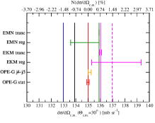
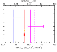
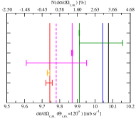
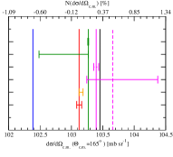
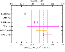
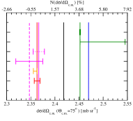
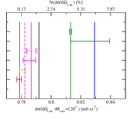
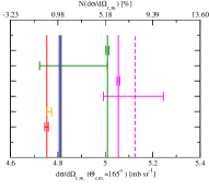
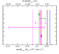
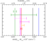
Figure 11: The $Nd$ elastic scattering differential cross section and various theoretical uncertainties at four scattering angles: $\theta_{\rm{c.m.}}=30^{\circ}$ (1st column), 75^∘ (2nd column), 120^∘ (3rd column), and 165^∘ (4th column) and at three scattering energies: $E=13$ MeV (the upper row), $E=65$ MeV (the middle row), and $E=200$ MeV (the bottom row). The x-axis at the bottom shows the values of the cross section, the x-axis at the top shows the relative difference of predictions with respect to the OPE-Gaussian results. The vertical lines show the position of the cross section obtained with the AV18 force (black line), the OPE-Gaussian force (red line), the E-M-N N⁴LO $\Lambda=500$ MeV force (green line), the CD-Bonn (blue line), the E-K-M N⁴LO $R$=0.9 fm force (magenta solid line), and the E-K-M N⁴LO $R$=1.0 fm force (magenta dashed line). The horizontal lines represent (from the bottom) the statistical error (red line), the difference between the OPE-Gaussian predictions with $j_{max}=5$ and $j_{max}=4$ (orange line) , the regulator dependence for the E-K-M force (magenta solid line), the truncation error for the E-K-M force (magenta dashed line), the regulator dependence for the E-M-N force (green solid line), and, at the top, the truncation error for the E-M-N potential (green dashed line), see text for details.

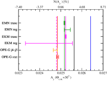
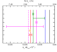
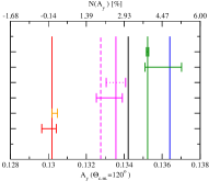
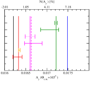
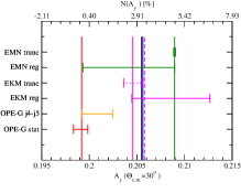
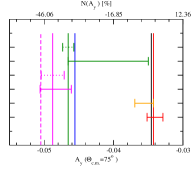
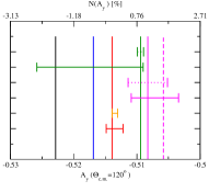
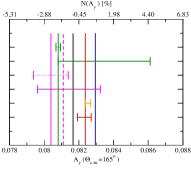
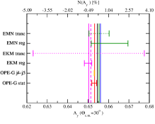
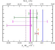
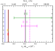
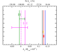
Figure 12: The same as in Fig. 11 but for the nucleon analyzing power A_y.

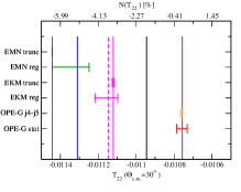
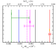
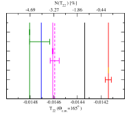
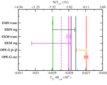
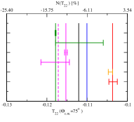
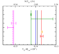
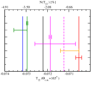
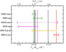
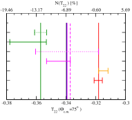
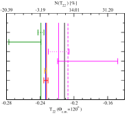
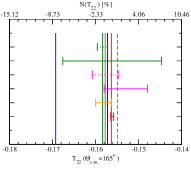
Figure 13: The same as in Fig. 11 but for the deuteron tensor analyzing power T₂₂.

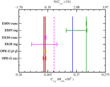
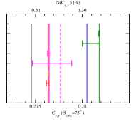
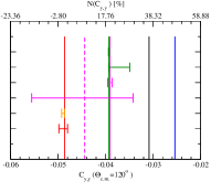
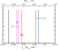
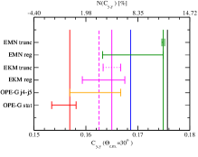
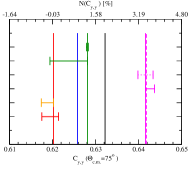
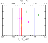
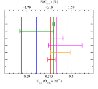
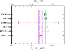
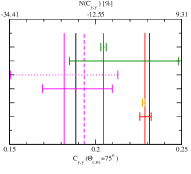
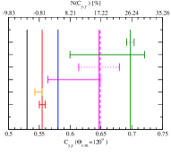
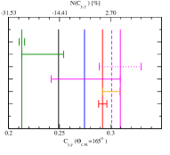
Figure 14: The same as in Fig. 11 but for the spin correlation coefficient C_y,y.

Next, it is interesting to compare the size of the theoretical errors presented in Figs. 11-14 to experimental errors of available data. In order not to leave the reader with the impression that the modern theoretical models of nuclear interactions yield a chaotic description of the $Nd$ scattering observables, in Fig. 15 we compare, in a few examples, previously presented predictions with the experimental results. This establishes an absolute scale in which one has to peer at the problem of discrepancies between various theoretical models.

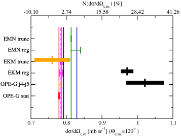
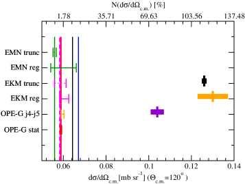
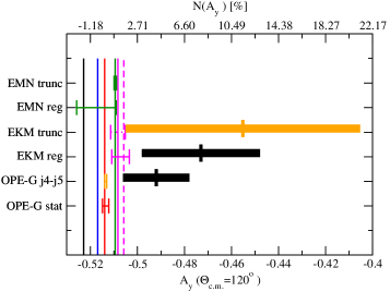
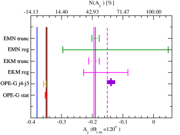
Figure 15: The same as in Fig. 11 ($d\sigma/d\Omega$, the upper row) and Fig. 12 (A_y, the bottom row) at $\theta_{\rm{c.m.}}=120^{\circ}$ for $E$=65 MeV (left) and $E$=200 MeV (right) but supplemented by the experimental points at angles near $\theta_{\rm{c.m.}}=120^{\circ}$. Vertical and thin horizontal lines are as in Fig. 11, and filled rectangles represent experimental data and their statistical errors, as in Figs. 5 and 6.

Examples given in Fig. 15 show various possible locations of theoretical predictions and data. The differential cross section at $E=65$ MeV and $E=200$ MeV at the scattering angle $\theta_{\rm{c.m.}}=120^{\circ}$ is shown in the upper row and the analyzing power A_y for the same angle and energies is displayed below. In the case of the cross section we see that at $E=65$ MeV there are discrepancies between various theoretical predictions and the data of different measurements. While the theoretical predictions are close one to each other, the data are scattered. One experimental point overlaps within its statistical error with some of the predictions, another one would be in agreement with predictions within 3$\sigma$ distance and the remaining experimental point is further from the data by more than its 3$\sigma$ uncertainty. At $E=200$ MeV a clear discrepancy between all predictions, which again are close together, and all data is observed. This discrepancy can be traced back to action of 3$N$ force at higher energies WitalaPRL ; Kuros . The picture is more complex for the analyzing power. Here, at $E=65$ MeV the experimental data and predictions differ by more than experimental error but they already agree within the 2$\sigma$ range. At $E=200$ the experimental statistical error is much smaller than the distances between various theoretical predictions and the uncertainties related to the chiral forces. Such a mixed pattern clearly calls for further work on reducing both the theoretical and experimental uncertainties to avoid misleading conclusions about the properties of the nuclear interactions. The presented here examples at one scattering angle only show that it is much more reliable to draw conclusions based on a comparison of predictions with data in a wider range of scattering angles and at different energies. Especially, these examples do not contradict strong effects of the 3$N$ force in the minimum of the differential cross section at higher energies WitalaPRL ; Kuros . Such conclusions are based on a systematic comparison of predictions with the data at numerous scattering angles and energies.

V Summary

We have employed the OPE-Gaussian potential of the Granada group to describe the elastic $Nd$ scattering at energies up to 200 MeV. The OPE-Gaussian potential is one of the first models of nuclear forces for which the covariance matrix of its free parameters is known. This gives an excellent opportunity to study the propagation of uncertainties from the 2$N$ potential parameters to 3$N$ observables. Therefore, for the same process, we also studied the statistical errors of our predictions.

The description of data delivered by the OPE-Gaussian force is in quantitative agreement with picture obtained using other $NN$ potentials, especially the AV18 model, which resembles by construction the OPE-Gaussian potential. We found only small discrepancies between predictions of these forces, especially at the highest energy investigated here, $E=200$ MeV, which can very probably originate from a slightly different behaviour of the phase shifts for the AV18 and the OPE-Gaussian potentials at energies above $\approx 150$ MeV. It should be noted that the procedure of fixing free parameters for the OPE-Gaussian force has been performed with big care for statistical correctness and covers new 2$N$ data not included when fixing the AV18’s parameters.

In order to obtain the theoretical uncertainty of our predictions arising from the uncertainty of the $NN$ potential parameters, we employed the statistical approach: we computed the $Nd$ scattering observables using fifty sets of the OPE-Gaussian potential parameters obtained from a suitable multivariate probability distribution. Next, we investigated a distribution of our results and adopted one of estimators of their dispersion, the $\frac{1}{2}\Delta_{68\%}$, as a measure of the theoretical statistical uncertainty. We also compared such statistical uncertainties for different observables with various types of theoretical errors, including the truncation errors and a dispersion due to using various models of the nuclear interaction. A comparison of uncertainties for the $Nd$ elastic scattering cross section and a few polarization observables for the OPE-Gaussian model with other types of theoretical uncertainties leads to important conclusions about currently used models of 2$N$ forces. First, all models of the $NN$ interaction considered here deliver qualitatively and quantitatively similar predictions for the $Nd$ elastic scattering observables. None of the interactions yields predictions systematically different from others and also no systematic grouping of predictions is observed. Secondly, we have found that in the case of the chiral forces, at small and medium energies, which are their natural domain of applicability, the dependence of predictions on the values of regulators dominates over another types of theoretical errors. At the highest investigated energy $E=200$ MeV which is at the limit of applicability of chiral forces, the truncation errors become important. It follows that during a derivation of the chiral models a constant attention should be paid to the regularization methods applied. Current attempts to solve this problem result in a range of regulator parameters too broad to make the chiral forces such a precise tool in studies of nuclear reactions as desired and expected. It would be very interesting to check if this conclusion remains valid after taking into account also consistent 3$N$ interaction at the investigated here order (N⁴LO) of chiral expansion.

Altogether the presented results clearly show that the modern nuclear experiments and theoretical approaches for the $Nd$ scattering achieved similar precision. Having in mind that many investigations are currently focused on studying subtle details of underlying phenomena, there is a need to further improve precision both in theoretical as well as in experimental studies. From the theoretical side a continuous progress in deriving consistent $NN$ and 3$N$ forces from the $\chi$EFT gives hope that this goal will be achieved.

- (1) K. Sekiguchi et al., Phys. Rev. C 96, 064001 (2017).
- (2) G. J. Weisel et al., Phys. Rev. C 89, 054001 (2014).
- (3) B. von Przewoski et al., Phys. Rev. C 74, 064003 (2006).
- (4) St. Kistryn et al., Phys. Rev. C 72, 044006 (2005).
- (5) C. R. Howell et al., Few-Body Syst. 16, 127 (1994).
- (6) The Editors, Phys. Rev. A 83, 040001 (2011).
- (7) H. Witała et al., Phys. Rev. C 63, 024007 (2001).
- (8) A. Kievsky et al., Phys. Rev. C 58, 3085 (1998).
- (9) Th. Cornelius et al., Phys. Rev. C 41, 2538 (1990).
- (10) D. Hüber et al., Phys. Rev. C 51, 1100 (1995).
- (11) J. L. Friar et al., Phys. Rev. C 42, 1838 (1990).
- (12) J. L. Friar, G. L. Payne, W. Glöckle, D. Hüber, and H. Witała, Phys. Rev. C 51, 2356 (1995).
- (13) E. Epelbaum, H. W. Hammer, and Ulf-G. Meißner, Rev. Mod. Phys. 81, 1773 (2009).
- (14) V. Bernard, E. Epelbaum, H. Krebs, and U. G. Meißner, Phys. Rev. C 77, 064004 (2008).
- (15) V. Bernard, E. Epelbaum, H. Krebs, and U. G. Meißner, Phys. Rev. C 84, 054001 (2011).
- (16) R. Machleidt and D. R. Entem, Phys. Rep. 503, 1 (2011).
- (17) D. R. Entem, R. Machleidt, and Y. Nosyk, Phys. Rev. C 96, 024004 (2017).
- (18) R. Navarro Pérez, J. E. Amaro, and E. Ruiz Arriola, Phys. Rev. C 88, 064002 (2013).
- (19) R. Navarro Pérez, J. E. Amaro, and E. Ruiz Arriola, Phys. Rev. C 89, 064006 (2014).
- (20) J. Dobaczewski et al., J. Phys. G: Nucl. Part. Phys. 41, 074001 (2014).
- (21) Focus issue Focus on Enhancing the Interaction Between Nuclear Experiment and Theory Through Information and Statistics of J. Phys. G: Nucl. Part. Phys. 42, 030301-034033 (2015), Editors: D. G. Ireland and W. Nazarewicz.
- (22) A. Ekström et al., Phys. Rev. Lett. 110, 192502 (2013).
- (23) R. Navarro Pérez, J. E. Amaro, and E. Ruiz Arriola, Phys. Rev. C 91, 054002 (2015).
- (24) R. Navarro Pérez, J. E. Amaro, and E. Ruiz Arriola, J. Phys. G: Nucl. Part. Phys. 43, 114001 (2016).
- (25) P. Reinert, H. Krebs, and E. Epelbaum, arXiv:1711.08821 [nucl-th].
- (26) R. J. Furnstahl, N. Klco, D. R. Phillips, and S. Wesolowski, Phys. Rev. C 92, 024005 (2015).
- (27) B. R. Barrett, P. Navratil, and J. P. Vary, Prog. Part. Nucl. Phys. 69, 131 (2013).
- (28) E. Epelbaum, H. W. Hammer, and Ulf-G. Meißner, Rev. Mod. Phys. 81, 1773 (2009).
- (29) E. Epelbaum, H. Krebs, and Ulf-G. Meißner, Eur. Phys. J. A 51, 26 (2015).
- (30) S. Binder et al., Phys. Rev. C 93, 044002 (2016).
- (31) R. Skibiński et al., Phys. Rev. C 93, 064002 (2016).
- (32) J. A. Melendez, S. Wesolowski, and R. J. Furnstahl, Phys. Rev. C 96, 024003 (2017).
- (33) E. Epelbaum, W. Glöckle, and Ulf-G. Meißner, Nucl. Phys. A 637, 107 (1998); 671, 295 (2000).
- (34) E. Epelbaum et al., Phys. Rev. C 66, 064001 (2002).
- (35) D. R. Entem and R. Machleidt, Phys. Rev. C 68, 041001(R), (2003).
- (36) E. Marji et al., Phys. Rev. C 88, 054002 (2013).
- (37) H. Witała, J. Golak, R. Skibiński, and K. Topolnicki, J. Phys. G: Nucl. Part. Phys. 41, 094011 (2014).
- (38) D. Rozpȩdzik et al., Phys. Rev. C 83, 064004 (2011).
- (39) R. Skibiński, J. Golak, D. Rozpȩdzik, K. Topolnicki, and H. Witała, Acta. Phys. Polon. B 46, 159 (2015).
- (40) E. Epelbaum, H. Krebs, and Ulf-G. Meißner, Phys. Rev. Lett. 115, 122301 (2015).
- (41) P. Maris et al., EPJ Web of Conf. 113, 04015 (2016).
- (42) S. Binder et al., arXiv:1802.08584 [nucl-th]
- (43) R. Navarro Pérez, A. Nogga, J. E. Amaro and E. Ruiz Arriola, J.Phys.Conf.Ser. 742, 012001 (2016).
- (44) R. B. Wiringa, V. G. J. Stoks, and R. Schiavilla, Phys. Rev. C 51, 38 (1995).
- (45) W. Glöckle et al., Phys. Rept. 274, 107 (1996).
- (46) W. Glöckle, The Quantum-Mechanical Few-Body Problem (Springer-Verlag, Berlin, 1983).
- (47) R. Navarro Pérez, E. Garrido, J. E. Amaro, and E. Ruiz Arriola, Phys. Rev. C 90, 047001 (2014).
- (48) S. S. Shapiro, M. B. Wilk, Biometrika 52, 591 (1965).
- (49) H. Witała, W. Glöckle, D. Hüber, J. Golak, and H. Kamada, Phys. Rev. Lett. 81, 1183 (1998).
- (50) J. Kuroś-Żołnierczuk et al., Phys. Rev. C 66, 024003 (2002).
- (51) S. Shimizu et al., Phys. Rev. C 52, 1193 (1995).
- (52) H. Rühl et al., Nucl. Phys. A 524, 377 (1991).
- (53) R. E. Adelberg, C. N. Brown, Phys. Rev. D 5, 2139 (1972).
- (54) G. Igo et al., Nucl. Phys. A 195, 33 (1972).
- (55) K. Ermisch et al., Phys. Rev. C 71, 064004 (2005).
- (56) J. Cub et al., Few-Body Syst. 6, 151 (1989).
- (57) R. V. Cadman et al., Phys. Rev. Lett. 86, 967 (2001).
- (58) S. P. Wells et al., Nucl. Instrum. Methods Phys. Res., Sect. A 325, 205 (1993).
- (59) K. Topolnicki, J. Golak, R. Skibiński, and H. Witała, Phys. Rev. C 96, 014611 (2017).