Variable blurred reflection in the narrow-line Seyfert 1 galaxy Mrk 493

Abstract

We examine a 200 ks XMM-Newton observation of the narrow-line Seyfert 1 galaxy Mrk 493. The active galaxy was half as bright as in a previous 2003 snapshot observation and the current lower flux enables a study of the putative reflection component in detail. We determine the characteristics of the 2015 X-ray continuum by first analyzing the short-term variability using model-independent techniques. We then continue with a time-resolve analysis including spectral fitting and modelling the fractional variability. We determine that the variability arises from changes in the amount of primary flux striking the accretion disk, which induces changes in the ionization parameter and flux of the blurred reflection component. The observations seem consistent with the picture that the primary source is of roughly constant brightness and that variations arise from changes in the degree of light bending happening in the vicinity of the supermassive black hole.

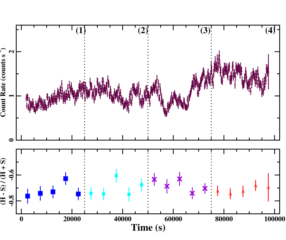
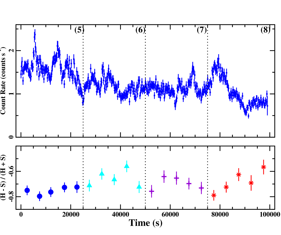
Figure 1: The 0.2-8.0 keV merged-MOS light curves for XMM15a (top left; maroon triangles) and XMM15b (top right; blue squares). The observations are separated by about $5$ days. The time segments adopted in the time-resolved analyses in Section 5 are shown. The XMM15 spectra were extracted every 25 ks for a total of four time bins per epoch. The divisions also serve as a rough flux-resolved analysis. Time-resolved hardness ratios compare the soft (0.35-0.5 keV) and hard (5-8 keV) bands (lower panels). The hardness ratios were derived with light curves binned by 5 ks. The symbols in Bin 1 (squares), Bin 2 (hourglasses), Bin 3 (crosses), Bin 4 (three-pointed stars), Bin 5 (circles), Bin 6 (triangles), Bin 7 (pluses), and Bin 8 (stars) will be used in the time-resolved analysis.

1 Introduction

Narrow-line Seyfert 1 (NLS1) galaxies are a class of active galactic nuclei (AGN) that are known for being exceptional at all wavelengths. On average, they have higher star formation rates (e.g. Sani et al. 2010) than the broad line Seyfert 1 galaxies. Some objects have even been identified with strong jet and $\gamma$-ray emission (e.g. Foschini et al. 2012, 2015). In X-rays, many objects possess spectra that are dominated by General relativistic effects (e.g. Fabian et al. 2009, 2013; Ponti et al. 2010) and exhibit extreme variability on various timescales (e.g. Grupe et al. 2007, 2012; Gallo et al. 2004). It is generally believed NLS1s possess smaller supermassive black holes than normal Seyfert 1s and are accreting at high Eddington rates.

Below about $2{\rm\thinspace keV}$, the X-ray spectra of Type 1 AGN show a soft-excess above the power law continuum, which is often enhanced in NLS1s. The nature of the soft excess is often debated (e.g. Ross & Fabian 2005, Crummy et al. 2006, Done et al. 2007, Done et al. 2012, Boissay et al. 2016) and one possibility is that the emission arises from blurred reflection of the primary source off the inner accretion disk (e.g. Ross & Fabian 2005). Measurements of reverberation lags lend support to this interpretation (e.g. Zoghbi et al. 2010).

The soft excess contains information on composition and the ionization of the inner disk. Modelling the soft excess and observing how the component various in conjunction to the primary source reveals information on the nature of the disk (e.g. densities) and the geometry (sizes) of the inner environment. The strong soft excess associated with NLS1s makes it possible to accurately study the inner disc properties and behaviour.

At low X-ray flux levels, the opportunity to study the nature of the accretion disk is improved as the continuum flux from the power law component is diminished and the reflection spectrum is enhanced (e.g. Miniutti & Fabian 2004). NLS1s are ideal to study AGN at low X-ray flux levels (specifically X-ray weak states) because they show strong variations from their nominal X-ray brightness. When they are X-ray bright, NLS1 tend to display simple, power law dominated spectra compared to when they are X-ray weak and exhibit more complex behaviour (e.g. Gallo 2006).

The NLS1 Mrk 493 is a local (z = 0.031) and bright AGN that is well studied at various wavelengths. However, detailed studies of the NLS1 in the X-rays are few. Mrk 493  has been viewed by Swift  every few years since 2005 (e.g. Grupe et al. 2010). On average, the source is about twice as bright as 1H 0707$-$495 and IRAS 13224$-$3809, but only various by a factor of about three over yearly timescales. There has been no detection of Mrk 493 in the 105-month BAT survey (Oh et al. 2018). A pointed 13.7 ks XMM-Newton observation in 2003 revealed an X-ray spectrum with a prominent soft-excess and Fe K$\alpha$ emission line. The source was categorized as a simple source by Gallo (2006) in that it did not exhibit significant spectral complexity.

A deep $190{\rm\thinspace ks}$ observation in 2015 with XMM-Newton  caught the source in a low X-ray flux state, which we report here. This work is organized as follows: Section 2 summarizes the data collection and reduction. Section 3 introduces the model-independent techniques first utilized to characterize the behaviour of Mrk 493 in the X-ray. A preliminary examination of the X-ray spectrum is completed in Section 4. The blurred reflection model is tested on the X-ray spectrum and used to describe the variability in Section 5. Discussion and conclusions follow in Section 6 and Section 7, respectively.

2 Observations and data reduction

The 2003 XMM-Newton observation (ObsID 0112600801; hereafter XMM03) was during revolution 0568 starting on 16 January 2003 and spanned 19 ks. The pn camera (Strüder et al. 2001) operated in large window mode and the two MOS detectors (Turner et al. 2001) operated in small window mode, all three detectors used a medium filter.

The first 2015 XMM-Newton observation (ObsID 0744290201; hereafter XMM15a) was during revolution 2786 starting on 24 February 2015 and spanned 97 ks. The second observation (ObsID 0744290101; hereafter XMM15b) was during revolution 2789 starting on 2 March 2015 and spanned 100.4 ks. The EPIC detectors all operated in small window mode with a medium filter for both 2015 observations. A log of the XMM-Newton  observations is presented in Table 1.

Table 1: Mrk 493 XMM-Newton data log for the single 2003 and two 2015 observations. Some background flaring was evident in XMM15b.

(1)	(2)	(3)	(4)	(5)
ObsID	Start Date	Duration	Instrument	GTI
(Designation)		(ks)		(ks)
0112600801	16/01/2003	19	pn	13
(XMM03)			MOS 1	18
			MOS 2	18
0744290201	24/02/2015	97	pn	66
(XMM15a)			MOS 1	92
			MOS 2	92
0744290101	02/03/2015	100	pn	69
(XMM15b)			MOS 1	87
			MOS 2	86

The Optical Monitor (OM; Mason et al. 2001) and Reflection Grating Spectrometers (RGS1 and RGS2; den Herder et al. 2001) observed simultaneously with the EPIC instruments during the 2015 epochs. The RGS were of low signal-to-noise and did not exhibit significant features. These data will not be discussed further. The OM data contain significant host-galaxy contribution and will be discussed elsewhere.

Data files from all epochs were processed to produce calibrated event lists using the XMM-Newton Science Analysis System (SAS) version 15.0.0 and latest calibration files at the time of writing. The data were examined for background flaring and pileup. Moderate flaring was seen throughout XMM15b and those time periods were ignored. No pileup was detected in either of the 2015 observations. Pileup was present in the 2003 pn data and this was corrected for. Source photons were extracted from a circular region 35 arcsec in radius and centred on the object. The background photons were extracted from an area 50 arcsec in radius close to the object and then scaled appropriately.

Single to quadruple events were selected for the MOS data while single and double events were selected for the pn. Events next to a bad pixel or the CCD edge were omitted (i.e. data quality flag set to zero). The MOS spectra from the 2015 data were limited to the 0.3 – 8.0 keV range because of high background at $E>$ 8 keV. The pn spectra of XMM15a were source dominated only between 0.3 – 6.5 keV, due to high background. The resulting mean count rates in the $0.3-10{\rm\thinspace keV}$ band for XMM03 were: 5.86${\rm\thinspace count}{\rm\thinspace s}^{-1}\,$ (pn), 1.41${\rm\thinspace count}{\rm\thinspace s}^{-1}\,$ (MOS 1), and 1.43${\rm\thinspace count}{\rm\thinspace s}^{-1}\,$ (MOS 2). For XMM15a mean count rates were: 1.88${\rm\thinspace count}{\rm\thinspace s}^{-1}\,$  (pn), 0.45${\rm\thinspace count}{\rm\thinspace s}^{-1}\,$  (MOS 1), and 0.45${\rm\thinspace count}{\rm\thinspace s}^{-1}\,$  (MOS 2) in the 0.3 – 8.0 keV band. For XMM15b the mean count rates were: 2.03${\rm\thinspace count}{\rm\thinspace s}^{-1}\,$  (pn), 0.50${\rm\thinspace count}{\rm\thinspace s}^{-1}\,$  (MOS 1), and 0.49${\rm\thinspace count}{\rm\thinspace s}^{-1}\,$  (MOS 2) in the same energy band as XMM15a.

In 2015, the MOS instruments provided good data over a wider bandpass than the pn because of higher background levels. The pn data were analysed throughout this work to examine for consistency between the instruments, but only the MOS data are reported.

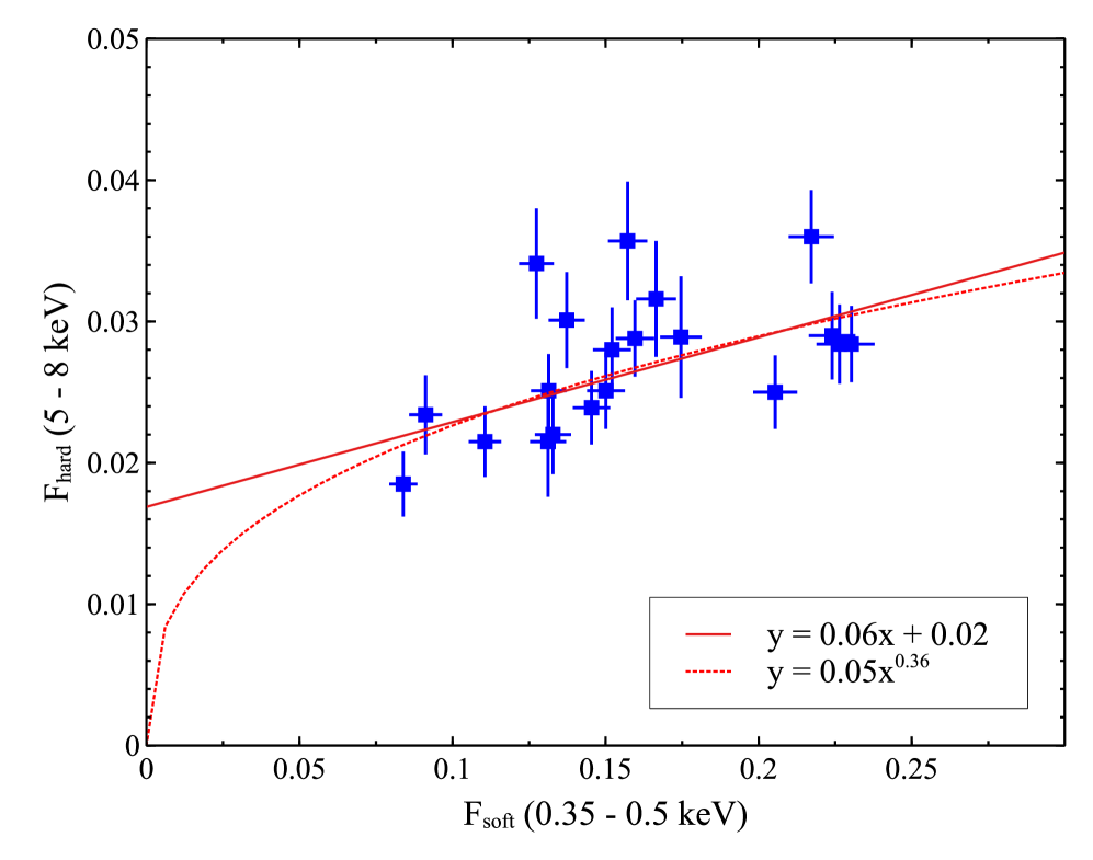
Figure 2: Flux-flux plots for XMM15a (top panel, maroon triangles) and XMM15b (lower panel, blue squares). Both curves were fit with linear (solid red line) and power law (dotted red line) models. A linear fit is sufficient to describe XMM15a (top panel), whereas neither model describes XMM15b well.

3 Model-Independent Analysis

Before delving into detailed multi-epoch spectroscopy, the 2015 Mrk 493 data are examined in a model-independent fashion. It is very common for several physical scenarios to describe spectra equally well (e.g. Bonson et al. 2015, Gallo et al. 2013, 2015) and so we hope to gather preliminary clues from the X-ray variability in Mrk 493 that may aid in later spectral analysis.

Source photons were extracted to create light curves in various energy bands between 0.2 – 10 keV for XMM03 and 0.2 – 8 keV for XMM15. At each epoch, the light curves from all EPIC instruments agree, therefore the MOS 1 and 2 light curves were combined, taking care to match the start and stop times.

The 2015, $0.2-8{\rm\thinspace keV}$ merged-MOS light curves are shown in Fig. 1. A simple visual inspection of the 2015 light curves show that the source varies by about 50 per cent and on timescales as short as $\sim$ 5 ks. Similar behaviour is found in 2003, though the duration of the observation was much shorter than in 2015.

Hardness ratios between the soft (0.35 – 0.5 keV) and hard (5 – 8 keV) bands in each observation were plotted with respect to time and reveal evidence of spectral variability (Fig. 1). No significant correlation is found between hardness ratio and count rate.

3.1 Flux-flux plots

To investigate the spectral variability, flux-flux plots comparing the $0.35-0.5{\rm\thinspace keV}$ and $5-8{\rm\thinspace keV}$ bands were created following Taylor et al. (2003) (Fig. 2). The light curves were binned by 5 ks.

The XMM15a flux-flux plot could be well fit with a linear model and a positive y-intercept ($\chi^{2}_{\nu}$= 0.93). This behaviour is consistent with a two-component continuum model where changes in the flux of a soft component (with constant shape) occur over a relatively constant hard component. In the case of MCG–6-30-15, the hard constant component was interpreted as blurred reflection (e.g. Taylor et al. 2003).

On the other hand, the XMM15b flux-flux plot is fit poorly with both a linear ($\chi^{2}_{\nu}$= 1.59) and power-law ($\chi^{2}_{\nu}$= 1.50) model. This suggests the variability is more complex, perhaps requiring multiple components to vary in shape and flux at the same time. The transition from the simple behaviour in XMM15a and the more complicated behaviour in XMM15b occurs in less than $\sim 5$ days (i.e. the time between epochs).

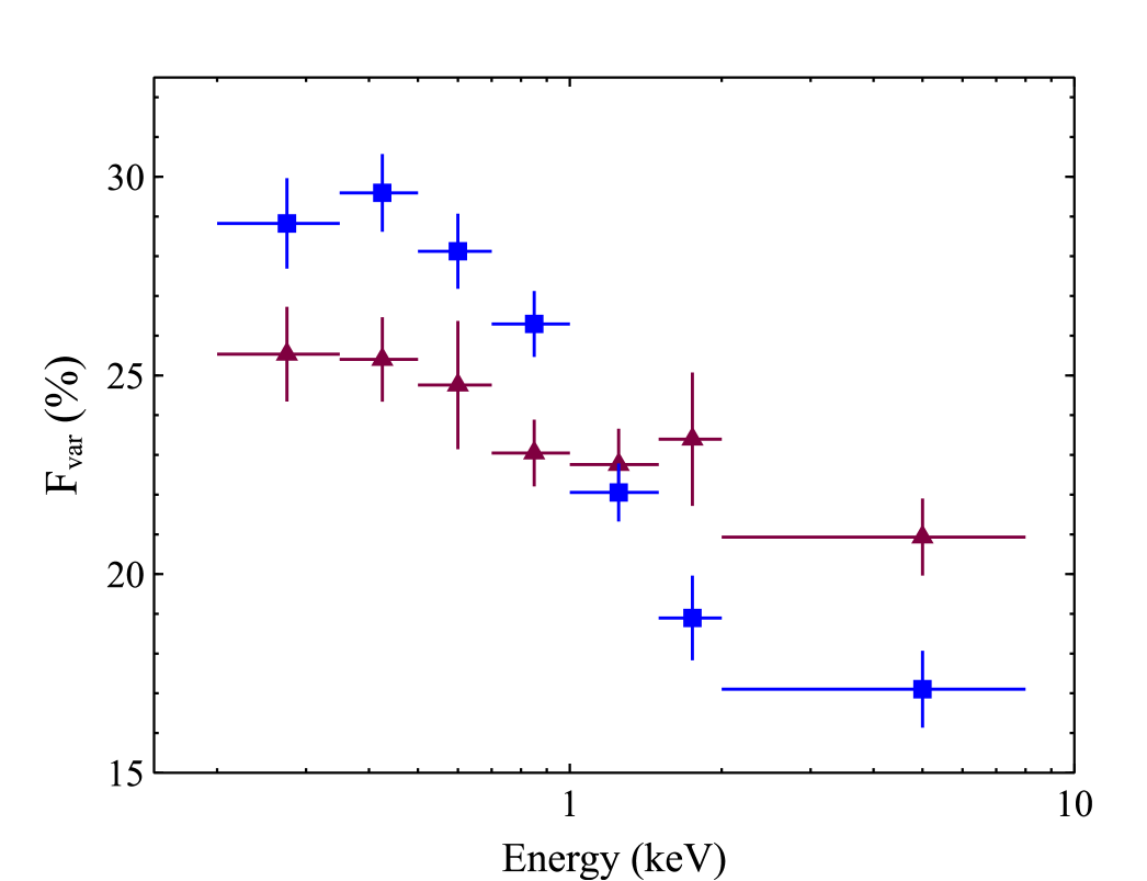
Figure 3: Fractional variability ($F_{\rm{var}}$) of the merged-MOS broad band light curves. Both epochs show increased spectral variability in the soft ($<$1 keV) band, with the variability in XMM15b being far more significant. As in Fig. 1, maroon triangles and blue squares represent XMM15a and XMM15b, respectively.

3.2 Fractional Variability

Root-mean-squared fractional variability ($F_{\rm{var}}$) analysis is used to quantify the variability intrinsic to a light curve while accounting for uncertainty (Edelson et al. 2002, Ponti et al. 2004). Mathematically,

$$F_{\rm{var}}=\frac{1}{\langle X\rangle}\sqrt{S^{2}-\langle\sigma^{2}_{\rm{err}}\rangle}$$ (1)

where $\langle X\rangle$ is the mean count rate, the total variance of the light curve is $S^{2}$, and $\langle\sigma^{2}_{\rm{err}}\rangle$ is the mean error squared. Calculating the $F_{\rm{var}}$ as a function of energy portrays the amplitude of the variations in different energy bands, therefore revealing spectral variability. The uncertainties are determined following Ponti et al. (2004).

The 2015 light curves were binned by $200{\rm\thinspace s}$ and a total of seven energy bins between $0.2-8.0{\rm\thinspace keV}$ were used to calculate the $F_{\rm{var}}$ spectrum. The $F_{\rm{var}}$ spectrum in XMM15a (Fig. 3, maroon triangles) shows a gentle increase in $F_{\rm{var}}$  toward lower energies. The trend is similar for XMM15b (Fig. 3, blue squares), but the changes between the soft and hard energy bands is more striking.

Similar $F_{\rm{var}}$ spectra are seen in other Type I Seyferts, which can often be attributed to changes in photon index of a varying power law or changes in the ionization parameter of a reflector (e.g. Gallo et al. 2013, Fabian et al. 2013, Bonson et al. 2015).

3.3 Principal Component Analysis

A powerful tool used in many scientific fields for multi-variable statistical analysis is Principal Component Analysis (hereafter PCA). PCA performs an eigenvalue decomposition in which a data set is modelled by a number of linear relationships that minimize low or redundant information. These linear relationships are the principal components and are made up of an eigenvalue or coefficient (also called a ‘loading’) along with its corresponding eigenvector. The principal components are not correlated by definition (see Feigelson & Babu 1992 for review). In other words, PCA looks for a collection of related variables in a data set that explains most of the variance and clumps them together into a single principal component. It then repeats the process, finding the second most influential variables (giving the second principal component), and so on until a data set is reduced to a few principal components that best model variance in the data.

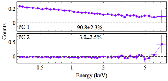
Figure 4: PCA normalized spectra using all the MOS data from 2003 and 2015. Data were binned by 10 ks.

PCA is a powerful technique as it is model-independent and has the ability to reduce a data set with hundreds of parameters down to a much more manageable size while retaining information. In the case of AGN timing analysis, PCA can be applied to isolate the uncorrelated variable components in an X-ray spectrum and quantify their variability. A PCA spectrum can then be created in order to identify which of the original spectral component(s) may be responsible for the majority of the variability (e.g. Parker et al. 2014a, Parker et al. 2014b, 2015).

Using the pca_public code, PCA was completed with data from all three XMM-Newton observations: the 2003 and both 2015 epochs. Observations were divided in $10{\rm\thinspace ks}$ intervals and a spectrum was created for each interval. PCA was conducted with data from: (i) the individual epochs, (ii) the 2015 epochs combined, and (iii) all three epochs combined. The PCA from each MOS camera at each epoch was consistent so the data were merged into a single spectrum.

Error bars were calculated by randomly perturbing the input spectra, recalculating the PCA, and finding the variance in the PCs themselves (Miller et al. 2007). The significance of individual components was assessed via log-eigenvalue (LEV) diagrams: the data were plotted by fractional variability as a function of eigenvector number. The data asymptotically approach a geometric series and components that fall above the trend outlined by the majority of points were considered significant (see Fig. 2 of Parker et al. 2014 as an example).

The PCA for the 2003 data was not informative given the short duration of the observation ($\sim 20{\rm\thinspace ks}$). The PCA of the individual 2015 data sets were found to be significant and comparable, therefore the data from XMM15a and XMM15b were combined. In the combined 2015 analysis the first three principal components were significant in the LEV diagram; however PC 2 and PC 3 only showed variations above $\sim 6{\rm\thinspace keV}$ and may be attributed to high background. PC1 accounted for 52.1$\pm$4.5 percent fractional variability and shows some sloping in the spectrum that decreases with increasing energy.

Finally, the high-flux state 2003 data are included with the low-flux 2015 data, and the PCA is calculated. The results are comparable with that of the 2015 PCA except that PC 1 is more significant accounting for 90.8$\pm$2.3 per cent of the spectral variability (Fig. 4). PC 2 is accounting for far less of the fractional variability in this case, $3.0\pm$2.5 per cent, with most of the variability at $>5{\rm\thinspace keV}$. This could be intrinsic as some curvature is seen in the spectra (Fig. 5) or it could be due to increased background emission.

Comparing Figure 4 to simulations in Parker et al. (2015), it seems as though the primary source of both short-term (hours) and long-term (years) variability in Mrk 493 is a change in normalization of some kind. The increased variability in the soft band is consistent with the results of the $F_{\rm{var}}$ analysis (Section 3.2) and in the difference spectrum that will be discussed in Section 4 (Fig. 5).

4 Preliminary examination of the mean spectra

We examine the average properties of the XMM03, XMM15a, and XMM15b spectra in a phenomenological manner. All spectral model fitting was performed using the X-ray spectral fitting package xspec v. 12.9.0. Model parameters are reported in the rest frame of the AGN ($z=0.03$) and a cosmology of $H_{\rm{0}}$ = 70$\hbox{${\rm\thinspace km}{\rm\thinspace s^{-1}}\,$}{\rm\thinspace Mpc}^{-1}\,$, $q_{\rm{0}}$ = 0, and $\Lambda_{\rm{0}}$ = 0.73 is assumed. All fits include a Galactic column density of $N_{\rm{H}}$ = 2.11$\times$$10^{20}$ $\rm{cm^{-2}}$ as determined from the LAB Survey (Kalberla et al. 2005) and modelled using the interstellar medium absorption model tbabs and abundances from Wilms et al. (2000). Errors on model parameters correspond to a 90 per cent confidence level.

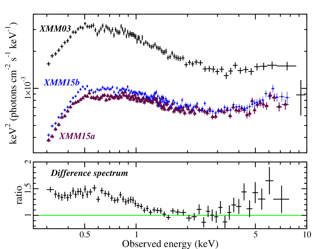
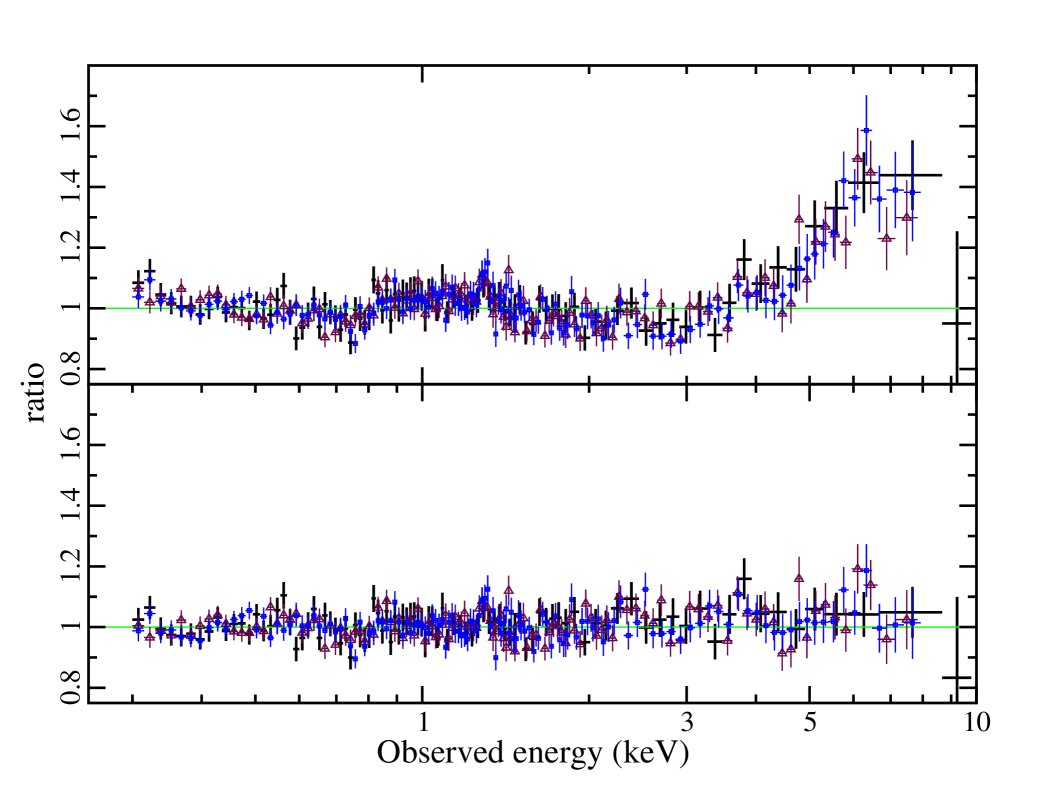
Figure 5: The unfolded spectra relative to a flat power law ($\Gamma=0$) are shown in the top panel. The 2015 observations (maroon triangles and blue squares) catch Mrk 493 in a dimmer state than in 2003 (black crosses). The spectra are steep and a soft excess below $\sim 1.5{\rm\thinspace keV}$ is prevalent at all epochs. The ratio of a difference spectrum (XMM03 – XMM15b) fitted with an absorbed power law between $1.5-4.5{\rm\thinspace keV}$ and extrapolated to higher and lower energies is shown in the second panel from the top. The ratio from fitting the three spectra with a black body plus power law model shows excess residuals between $5-8{\rm\thinspace keV}$ in all three epochs (second panel from bottom). The lowest panel depicts the ratio from fitting the spectra with a broad Gaussian profile in addition to the black body plus power law continuum.

In the top panel of Fig. 5, the three unfolded spectra relative to a flat power law ($\Gamma=0$) are shown to demonstrate changes between the epochs. At all three epochs the spectrum is rather steep and a strong soft excess is clearly present. The dimmer 2015 spectra show curvature with increasing energy peaking between $6-7{\rm\thinspace keV}$. Even though the 2015 spectra are obtained only 5 days apart, there are obvious changes in the soft excess during that time.

A difference spectrum is created between the 2003 bright state and one of the 2015 spectra (XMM15b). The difference spectrum is fitted with an absorbed power law ($\Gamma=2.7$) between $1.5-4.5{\rm\thinspace keV}$ and extrapolated to lower and higher energies. The ratio of this fit is shown in Fig. 5 (second panel from top), clearly portraying changes in the soft excess and above $5{\rm\thinspace keV}$ in the Fe K$\alpha$ band.

Each of the three spectra is fitted independently with a black body plus power law model. The ratios of the fit are shown in Fig. 5 (second panel from bottom). Clear residuals exist in the Fe K$\alpha$ band that are improved when a broad Gaussian profile is added to each model (Fig. 5, lower panel). Overall, the black body plus power law continuum with a broad Gaussian profile fits the three spectra well ($\chi^{2}_{\nu}$ $\sim 1.05$). The parameters are typical of most NLS1s fitted in this manner. The temperature of the black body component is $\approx 110{\rm\thinspace eV}$. The power law component is steep and changes significantly from $\Gamma\sim 2.68$ in 2003 to $\sim 2.45$ in 2015. The Gaussian profile is centred at $\sim 5{\rm\thinspace keV}$ and is broad ($\sigma>1{\rm\thinspace keV}$) in all three spectra.

Based on the best-fit model above the corresponding, unabsorbed fluxes in the $2-10{\rm\thinspace keV}$ ($0.3-10{\rm\thinspace keV}$) band are $3.57\rm(15.2)$, $1.72\rm(5.16)$ and $1.89\rm(5.75)\times 10^{-12}\hbox{${\rm\thinspace erg}{\rm\thinspace cm}^{-2}{\rm\thinspace s}^{-1}\,$}$ for XMM03, XMM15a, and XMM15b, respectively. The $2-10{\rm\thinspace keV}$ luminosity is approximately $3.6$ and $1.8\times 10^{42}\hbox{${\rm\thinspace erg}{\rm\thinspace s}^{-1}\,$}$ in 2003 and 2015, respectively.

Notably, in 2015 the primary differences in the spectra lie in the soft excess. While the flux of the broad Gaussian profile remains comparable in both 2015 spectra the soft excess (black body component) is about three-times brighter in XMM15b than it is in XMM15a. The results from this simple examination of the spectra seems consistent with the the light curve analysis in Sect. 3 that show spectra variability is more significant at lower energies.

While differences are present between 2003 and 2015 (e.g. $\Gamma$ and normalization), from this point, the focus of the work will be on understanding the rapid spectral variability in the high quality 2015 data.

Table 2: The blurred reflection model for the simultaneous fit to the 2015 spectra. The merged-MOS data were fit between 0.3-8 keV. Parameters that are linked between epochs are shown with dots in column (4). The reflection fraction ($R$) is the ratio of total fluxes (reflection/continuum) between $0.1-100{\rm\thinspace keV}$. The reported unabsorbed flux is in the $2-10{\rm\thinspace keV}$ band.

(1)	(2)	(3)	(4)
Model	Model	XMM15a	XMM15b
Component	Parameter
Power	$\Gamma$	2.14$\pm$0.03	…
Law	model flux	5.96$\times 10^{-4}$	…
	($\rm{ph}{\rm\thinspace cm}^{-2}{\rm\thinspace s}^{-1}\,$)
Blurred	$q_{1}$	7.50$\pm$1.50	$6.62^{+1.11}_{-2.88}$
Reflector	$R_{\rm{in}}$ ( $R_{\rm g}$)	$1.25^{+0.34}_{-0.02}$	…
	$\theta$ (deg)	$53^{+6}_{-23}$	…
	$A_{\rm{Fe}}$ (solar)	$0.53^{+0.09}_{-0.07}$	…
	$\Gamma$	$2.14$	…
	$\xi$ (${\rm\thinspace erg}{\rm\thinspace cm}{\rm\thinspace s}^{-1}\,$)	$1005^{+119}_{-242}$	$800^{+228}_{-128}$
	model flux	2.53$\times 10^{-3}$	2.94$\times 10^{-3}$
	($\rm{ph}{\rm\thinspace cm}^{-2}{\rm\thinspace s}^{-1}\,$)
	$R$ ($F_{\rm{ref}}$ / $F_{\rm{pl}}$)	2.58$\pm$0.09	3.63$\pm$0.07
Flux	$2-10{\rm\thinspace keV}$	$1.70\times 10^{-12}$	$1.83\times 10^{-12}$
	(${\rm\thinspace erg}{\rm\thinspace cm}^{-2}{\rm\thinspace s}^{-1}\,$)
Fit Statistic	$\chi^{2}_{\nu}$ /dof = 1.05 / 786

5 The Blurred Reflection Scenario for 2015

The analysis in the previous sections suggests the variability in 2015 is mainly driven by changes in normalization of a primary continuum component (e.g. Fig. 2 and 4), though the flux-flux plot in XMM15b indicate other factors are at work as well. The X-ray spectra in the low-flux 2015 epochs is typical of most NLS1 and well described by a power law plus black body and a broad Gaussian profile at $\sim 6{\rm\thinspace keV}$ that resembles a relativistic iron line profile. The predominant difference between the 2015 spectra is the strength of the soft excess. Here, we consider if the blurred reflection model (e.g. Ross & Fabian 2005) can describe the spectra and spectral changes seen in 2015.

5.1 Fitting the 2015 average spectra

Relativistic blurred reflection is expected to be seen in objects in which there is an unobstructed view of the AGN central engine: namely, Type I sources. In essence, the primary, non-thermal X-rays from the corona are reprocessed in the accretion disk via a combination of processes including fluorescence, Compton scattering, and bremsstrahlung. This reflected emission is blurred due to the Doppler effects in the disk and relativistic effects close to the black hole. In addition, the extreme gravitational forces close to the supermassive black hole can enhance emission from the inner regions by light bending (e.g. Miniutti & Fabian 2004). This boosted and smoothed reflection from the inner disk region forms the observed soft-excess emission below $\sim$ 1 keV seen in most Type I sources.

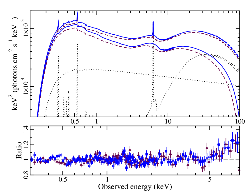
Figure 6: Top: The best blurred reflection model, shown between $0.1-100{\rm\thinspace keV}$, was simultaneously fit to the merged-MOS data of both 2015 observations. The model components corresponding to XMM15a are shown as maroon, dashed curves and those corresponding to XMM15b are shown as solid, blue curves. The distant reflector and power law are shown as dotted, black curves. These are non-variable and common to both epochs. Bottom: The model residuals (data / model) between $0.3-8{\rm\thinspace keV}$. Maroon triangles and blue squares correspond to XMM15a and XMM15b data, respectively. Note the different energy scales used in the two panels.

Initially, spectra from XMM15a and XMM15b were examined separately to search for gross inconsistencies before fitting both spectra simultaneously. The disk reflection model reflionx (Ross & Fabian 2005) was utilized. The reflection spectrum was modified for motions in the disc close to the black hole with the blurring kernel kdblur2, which incorporates a broken power law for the emissivity profile. The following parameters were linked between the epochs: inner disk radius ($R_{\rm{in}}$), inclination angle ($\theta$), and iron abundance ($A_{\rm{Fe}}$). The blurring parameters were also linked and the break radius ($R_{\rm{br}}$) and outer emissivity index ($q_{2}$), which were not well constrained when allowed to vary freely, were fixed to 10 $R_{\rm g}$ ($R_{g}=GM/c^{2}$) and 3, respectively.

In addition, both spectra seemed to require a narrow core at $\sim 6.4{\rm\thinspace keV}$ that is modelled as distant, un-blurred reflection (e.g. from a torus). The components of the distant reflector are identical for both 2015 spectra. To describe a neutral, distant reflector, such as that from a cold torus, the ionization parameter was fixed at $\xi$ = 1${\rm\thinspace erg}{\rm\thinspace cm}{\rm\thinspace s}^{-1}\,$ and the iron abundance was set to solar. The photon index of the power law source illuminating the distant reflector was fixed at $\Gamma$ = 1.9, the canonical value for AGN (e.g. Nandra & Pounds 1994). There is no reason to assume that the radiation incident on the distant reflector will be the same as that from the primary component, but allowing $\Gamma$ to be linked to the power law continuum did not noticeably alter the fit. The normalization was the only model component allowed to vary and it was linked between the epochs.

Both spectra in 2015 are well-described with the single blurred reflector model ($\chi^{2}$ / dof = 825 / 784). Slight positive residuals remained at $E>6{\rm\thinspace keV}$, which may be due to the onset of significant background emission or true spectral variability. A variable component above $6{\rm\thinspace keV}$ is seen in the PCA (Fig. 4). We also note the spectrum above $6{\rm\thinspace keV}$ is better fit when we consider time-resolved spectroscopy in Section 5.2, suggesting the difficulty fitting the average spectrum may be from rapid spectral variability.

If the primary components ($\Gamma$ and normalization) were linked between XMM15a and XMM15b, the fit quality was comparable ($\chi^{2}$ / dof = 826 / 786) and the residuals are unchanged. Therefore, in the final model the power law component is linked between the epochs (Fig. 6; Table LABEL:BR+DR_fit).

The parameters for the best-fit blurred reflector model are listed in Table LABEL:BR+DR_fit. Based on the fits to the two average spectra, Mrk 493 is reflection dominated in 2015 when it is at a relatively low-flux interval. The difference between XMM15a and XMM15b can be explained primarily with changes in the flux and ionization parameter of the blurred reflector. We examine this in further detail in the following sections.

The model-predicted $14-195{\rm\thinspace keV}$ flux is approximately $2.4\times 10^{-12}\hbox{${\rm\thinspace erg}{\rm\thinspace cm}^{-2}{\rm\thinspace s}^{-1}\,$}$, which is consistent with the null-detection in the 105-month Swift -BAT survey (Oh et al. 2018).

5.2 Time-Resolved Spectroscopy

Time-resolved spectra are created for the consecutive $25{\rm\thinspace ks}$ segments that are shown in Fig. 1. There are four spectra created for XMM15a (numbered $1-4$) and four spectra for XMM15b (numbered $5-8$) (see Fig. 1 and 7).

An absorbed power law is fit to each time-resolved spectrum between $2-8{\rm\thinspace keV}$. The photon index is linked between the time bins at each epoch, while the normalization is allowed to vary. The fit is then extrapolated to $0.3{\rm\thinspace keV}$. The residuals from this fit are displayed in Fig. 7, showing the spectral changes as a progression from one bin to the subsequent bin. In addition to changes in power law flux, Fig. 7 demonstrates there are also difference in the soft-excess (e.g. Bin 1 - 2 and Bin 4 - 5) and in the Fe K$\alpha$ band (e.g. Bin 5 - 6 and Bin 6 - 7). Interestingly, there is some indication that changes in the soft-excess may precipitate changes in the Fe K$\alpha$ band. For example, increased soft-excess emission in Bin 5 is followed by enhance emission between $5-6{\rm\thinspace keV}$ in Bin 6.

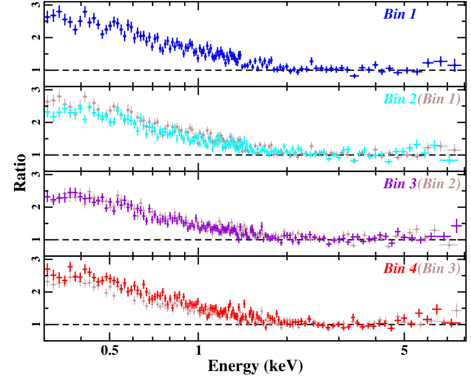
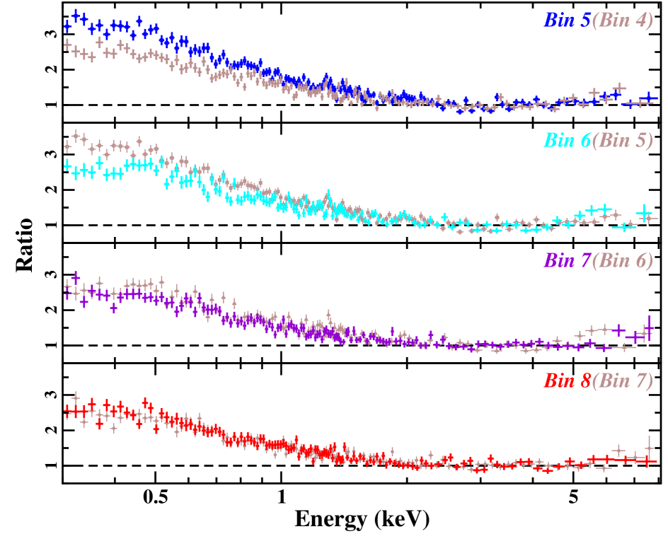
Figure 7: A power law model is fit between $2-8{\rm\thinspace keV}$ to all time-resolved spectra while keeping the photon index linked and the normalisation free to vary. The model is extrapolated to $0.3{\rm\thinspace keV}$ and the residuals (ratios) are shown for the time bins in XMM15a (left panel) and XMM15b (right panel). The residuals in each bin are compared to those in the preceding time segment (faded brown data) to highlight changes from one spectrum to the next.

The blurred reflection model is used to fit the eight time-resolved spectra. Considering the parameters that changed in fitting the 2015 average spectra (Sect. 5.1), the power law normalization, inner emissivity index, disk ionization, and reflector normalization are permitted to vary between time bins. Allowing the photon index to be free also improves the fit, though the value of the parameter did not change significantly from one spectrum to the next. The model reasonable fit all eight time-resolved spectra ($\chi^{2}$/dof = 1945 / 1899).

A Markov Chain Monte Carlo (MCMC) method was used to estimate the uncertainties for the time-resolved spectral model via an open-source algorithm developed by Foreman-Mackey et al. (2013) utilizing the original Goodman & Weare (2010) method. The xspec-friendly program, xspec_emcee, was developed by Jeremy Sanders and is publicly available. The MCMC fitting was run with 76 walkers and 10,000 iterations. The best-fit parameter values were used as the peak of the MCMC probability distributions and the errors were the widths of those distributions. The first 1000 steps were burned to ensure truly random initial conditions. Only the photon index, power law normalization, blurred reflection ionization, and the inner emissivity index were allowed to vary. The inclination angle and iron abundance were linked between all the spectra, but allowed to vary. The flux of the power law and that of the blurred reflector were calculated between 0.1 – 100 keV to track reflection fraction ($R$) as well.

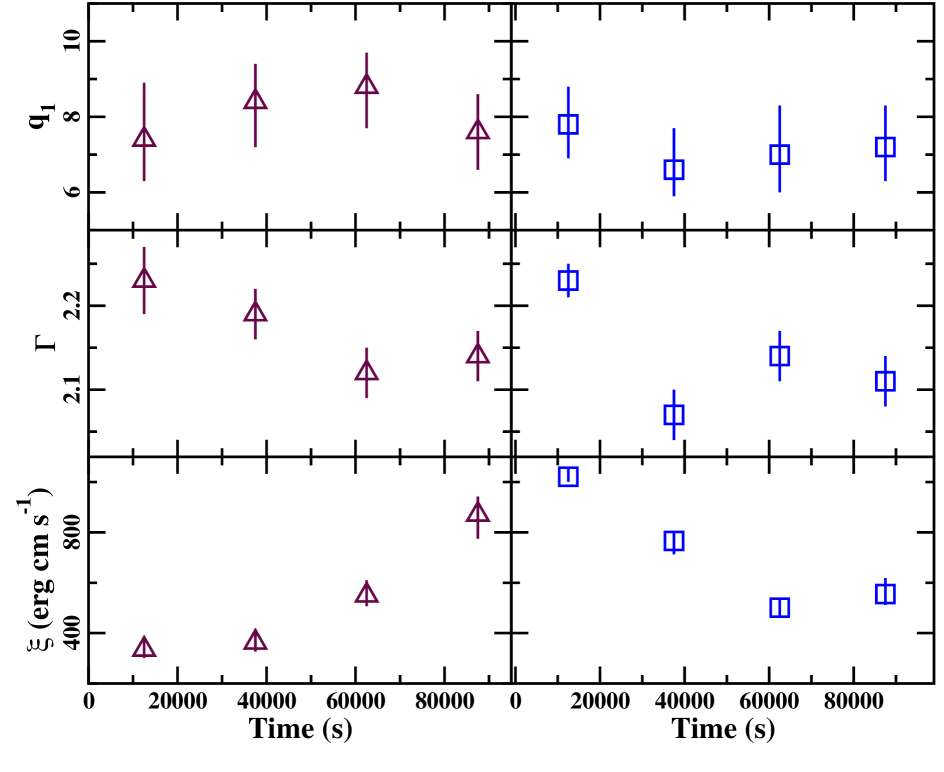
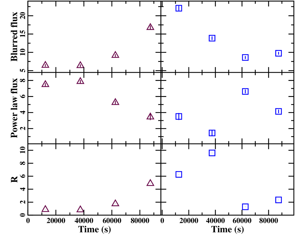
Figure 8: Trends extracted from the simultaneous fitting of time-resolved spectra with the blurred reflection model. Data from XMM15a (maroon triangles) and XMM15b (blue squares) are binned in approximately $25{\rm\thinspace ks}$ bins as shown in Fig. 1. Power law and blurred reflector fluxes are given in units of $10^{-4}$ and $10^{-3}$ ph cm^-2 s^-1, respectively.

A time series was created for each fit parameter to track changes from one bin to the next (Fig. 8). We see that while the inner emissivity index remains relatively constant within uncertainties, the other three parameters show significant variability across the 25 ks time bins. The power law photon index does vary, but by only about $\pm 5$ per cent. Disk ionization more than doubles between the start of XMM15a and the start of XMM15b, before dropping again to nearly its starting values. Power law normalization shows an opposite trend to that of disk ionization: dropping from its starting value to a minimal value in Bin 2, before climbing once again.

The most variable parameters in Fig. 8 are compared to each other to search for correlations (Fig. 9). There is a clear inverse trend between the flux of the power law component and the flux of the blurred reflector (lower panel of Fig. 9) and a tight correlation between the ionization parameter and the blurred reflector flux (upper panel of Fig. 9). The trends are consistent with the light bending interpretation (e.g. Miniutti & Fabian 2004). If photons from power law component are directed toward the disk due to the curve space-time around the black hole, the direct power law flux reaching the observer drops as more photons strike the inner disk, increasing the flux from the reflection component. Since more photons are striking the inner disk, the ionisation parameter will consequently increase as well. The trend is also apparent in the reflection fraction ($R$), which is highest during moments of low power law flux. On average, $R>1$ indicating Mrk 493 is reflection dominated.

The described light bending scenario could occur in a simple lamp-post geometry where the source (power law emitter) height above the disk is changing. We considered this possibility by modelling the spectra of Bin 1 and Bin 5, which have diverse blurred reflection parameters, with the xspec model relxilllp (Garcia et al. 2014). The source height is a free parameter in the relxilllp model. Unfortunately, the model could not significantly distinguish different source heights in Bin 1 and 5. While the resulting values are consistent with the scenario above (i.e. lower source height in Bin 5) the measurements are comparable within uncertainties.

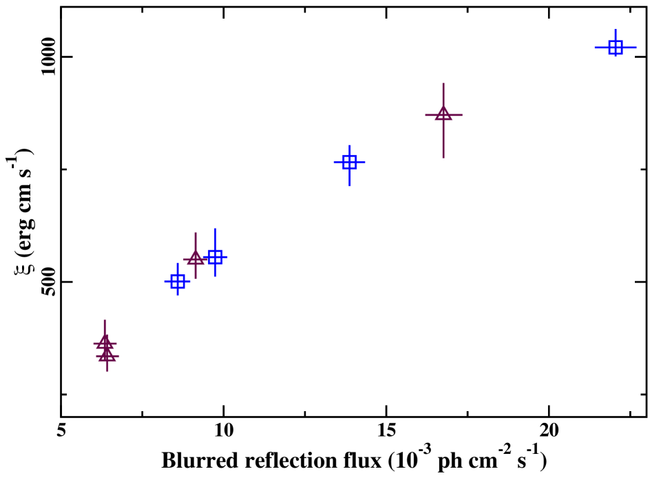
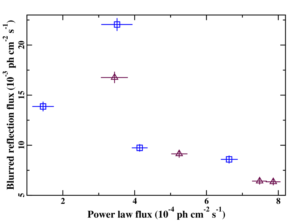
Figure 9: Comparison between measured parameters in the time-resolved spectral analysis. The disk ionization parameter is compared to the flux from the blurred reflector in the top panel. The blurred reflector flux and power law flux are compared in the lower panel. Data from XMM15a and XMM15b are shown as maroon triangles and blue squares, respectively.

5.3 Time-Resolved $F_{\rm{var}}$ Modelling

Fractional variability spectra were created for each of the eight time segments to investigate how the $F_{\rm{var}}$  changes over the 2015 observations. These time-resolved $F_{\rm{var}}$ spectra are shown in Fig. 10 using the same symbols and colours as defined in Fig. 1 to identify data in different time segments. The combination of the time-resolved spectra appear generally consistent with the average $F_{\rm{var}}$ spectra in Fig 3.

The time-resolved $F_{\rm{var}}$ spectra are approximately flat during all time segments, but the most significant spectral variability and largest amplitude variations are seen in Bin 3 and Bin 8. The segments correspond to periods when Mrk 493 was at its lowest average flux. During these more active segments, the amplitude of the variations are enhanced at all energies, but the majority of the variability is in the soft excess below $\sim$ 1 keV.

To investigate possible scenarios that could produce the different time-resolved $F_{\rm{var}}$ spectra, we simulate one hundred spectra based on the best-fit blurred reflection model (Sect. 5.1) allowing only one parameter to vary randomly. The parameters tested were the photon index ($\Gamma$), power law normalization ($PL_{\rm{n}}$), and the disk ionization parameter ($\xi$). From these simulated spectra, theoretical $F_{\rm{var}}$ spectra were calculated and overplotted on the time-resolved $F_{\rm{var}}$ spectra of Mrk 493 (Fig. 10).

It is not possible to reproduce the flat $F_{\rm{var}}$ spectra seen during most of the time segments by allowing only one parameter to vary at a time. Most likely, multiple parameters need to vary together in some manner to reproduce the constant variations across the entire energy band. For example, Fig. 8 shows how the blurred reflection and power law flux (i.e. normalization) are anti-correlated during the observation.

The enhanced variability at lower energies is most likely achieved by changing the ionization parameter. Varying the photon index can not reproduce the large amplitude changes at low energies since the soft component (i.e. blurred reflection in our model) would dampen the variations. Again, the mostly likely scenario is that multiple components need to change simultaneously to accurate recreate the $F_{\rm{var}}$ spectra.

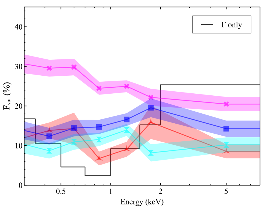
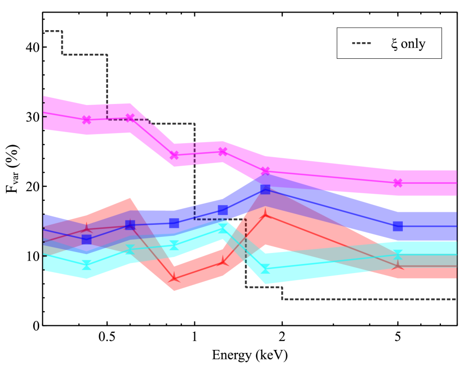
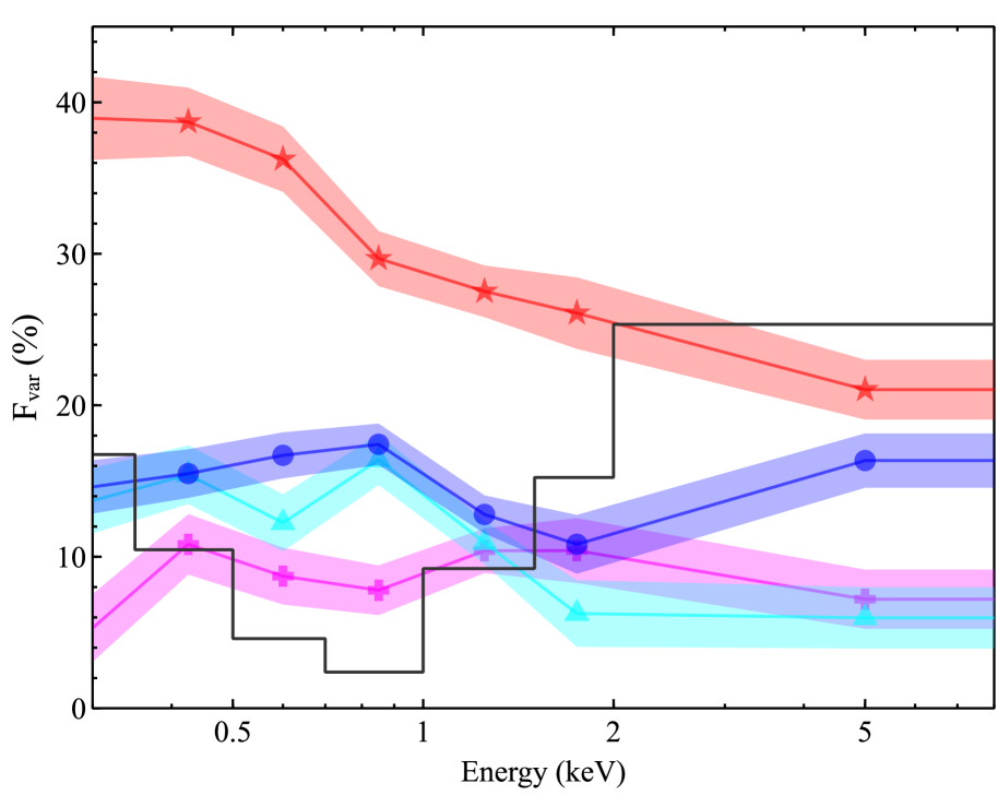
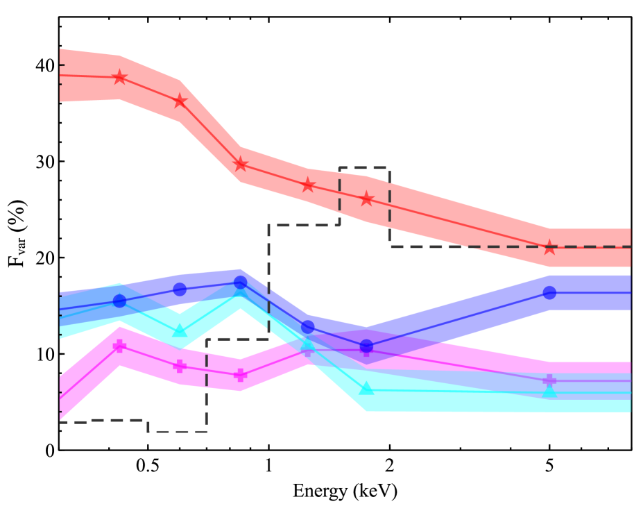
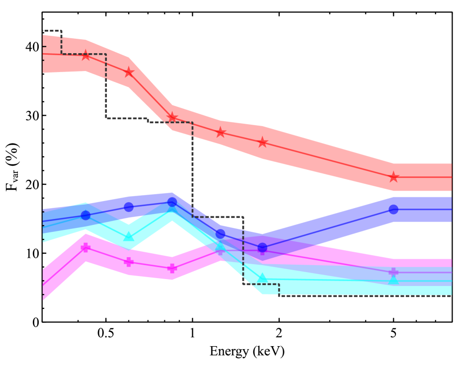
Figure 10: Time-resolved $F_{\rm{var}}$ spectra for each time segment shown in Fig. 1. Data of XMM15a and XMM15b are shown in the top and lower panels, respectively. Symbols and colours correspond to the segments as shown in Fig. 1. The most variable segments correspond to Bin 3 (purple crosses) during XMM15a and Bin 8 (red stars) during XMM15b. Theoretical $F_{\rm{var}}$ spectra are overplotted as black curves in each panel. The inset in the top panels identifies the parameters that are assumed to vary to created the simulated $F_{\rm{var}}$ for that column. From left-to-right, the variable parameters are the photon index ($\Gamma$, solid), power law normalization ($PL_{\rm{n}}$, dashed), and disk ionization ($\xi$, dotted). A simple scenario in which only one model parameter changes at a time does not reproduce the spectral variability in Mrk 493.

6 Discussion

This is the first in-depth examination of the NLS1 galaxy, Mrk 493, with XMM-Newton . Two, approximately $100{\rm\thinspace ks}$ observations separated by $\sim 5$ days, show the source to have a typical NLS1 X-ray spectrum with a strong soft excess and broad excess emission in the Fe K$\alpha$ band. The average spectra are well-described by a blurred reflection model that indicates the AGN is reflection dominated, like many NLS1s (e.g. Fabian et al. 2009, 2013; Gallo et al. 2004).

The AGN appears to be in a low flux interval, which would be consistent with the reflection dominated scenario (e.g. Gallo 2006). For example, the 2015 data of Mrk 493 were compared to a 2003 snap-shot observation when the AGN was more than twice as bright (Fig. 5). The PCA utilizing 2003 and 2015 data (Fig. 4) is compared to models generated by Parker et al. (2015) and suggest the primary changes are in the normalization and pivot of the power law component.

Time-resolved spectroscopy, PCA, flux-flux plots, and $F_{\rm{var}}$ modelling indicate the short-term variability during the 2015 XMM-Newton  observations can not be described by variability in a single component. Changes in the normalization of the power law and blurred reflector are necessary, but strong changes in the soft excess emission suggests the ionization parameter of the blurred reflector fluctuates as well.

Interestingly, changes are also seen in the Fe K$\alpha$ band. For example, in Bin 6 of the time-resolved spectroscopy (Fig. 7), enhanced emission is seen between $5-6{\rm\thinspace keV}$ that succeeds changes in the soft excess in Bin 5. These changes in the Fe K$\alpha$ emission could originate along with overall changes in the continuum, but could also arise from spots or annuli on the disk that momentarily brighten or infalling material (e.g. Bonson 2017, Yaqoob et al. 2003, Giustini et al. 2017).

The time-resolved spectroscopy shows the varying model parameters are the blurred reflector and power law flux, and the ionization parameter. Comparing the parameters, we find a strong correlation between the ionization parameter and the flux of the blurred reflector as well as a negative trend between the flux of the reflector and power law (Fig. 9). These trends seem consistent with the light bending scenario (e.g. Miniutti & Fabian 2004). If we consider a standard lamp-post geometry where the primary source is an isotropic emitter of roughly constant luminosity situated above the black hole, but allowed to vary in height, then when it is in the strong gravity environment close to the black hole, most of the power law photons will be directed toward the inner accretion disk. The primary (power law) source will appear dimmer to the distant observed while the reflected emission will appear relatively enhanced. As more continuum photons are striking the inner accretion disk, the ionization parameter of the reflector will increase producing the correlations we observe in Fig. 9.

The described scenario predicts changes in the inner emissivity index ($q_{1}$) of the disk that are not clearly observed in the time-resolved spectra (Fig. 9). However, this could be a data quality issue. The parameter $q_{1}$ is poorly constrained with the current data. Values in the time-resolved analysis are uncertain at about $\pm 20$ per cent and best-fit values range from $q_{1}\sim 6-9$. In addition, the break radius was not well constrained when it was free to vary so it was fixed at $10$ $R_{\rm g}$. The break radius and emissivity index are coupled in the lamp-post scenario and the break radius will become smaller when $q_{1}$ increases.

Though the primary source is treated as a point in this lamp-post scenario, it could equivalently be described as a compact spherical corona or the base of a jet. Both structures could be rather dynamic generating the power law variability (e.g. Wilkins et al. 2014, 2015; Wilkins & Gallo 2015) driving the changes in the blurred reflector. Distinguishing these origins is possible (Wilkins & Fabian 2012; Gonzalez et al. 2017) and should be attempted with higher quality data in the $2-10{\rm\thinspace keV}$ band.

7 Conclusions

We examined the characteristics of the X-ray continuum of the NLS1 galaxy, Mrk 493, by considering both the long- and short-term variability. Data from XMM-Newton merged-MOS instruments were primarily utilized due to high background in the pn, however the pn data were processed alongside all investigations to confirm results.

The 2015, low-flux spectra of Mrk 493 are well-fit with a blurred reflection model that is reflection dominated. However, the variability within the 2015 observation is complex and can not be described by fluctuation in a single component. In addition to changes in brightness of the power law and reflector, variations in the ionisation parameter of the blurred reflector are needed to fit the soft excess.

The behaviour displayed by Mrk 493 in 2015 suggests the X-ray source is compact and that the NLS1 will be a useful source for studying the inner accretion disk around supermassive black holes.

References

- [1] Boissay R., Ricci C., Paltani S., 2016, A&A 588, 19.
- [2] Bonson K. A critical examination of Seyfert 1 X-ray spectroscopy, 2017, Thesis (PhD.), Saint Mary’s University
- [3] Bonson K., Gallo L. C., Vasudevan R., 2015, MNRAS 450, 857.
- [4] Crummy J., Fabian A. C., Gallo L., Ross R. R., 2006, MNRAS 365, 1067
- [5] den Herder J. W. et al. 2001, A&A, 365, 7.
- [6] Done C. & Nayakshin S. 2007, MNRAS 377, L59.
- [7] Done C., Davis S. W., Jin C., Blaes O., Ward M., 2012, MNRAS 420, 1848.
- [8] Edelson R. et al. 2002, ApJ 568, 610.
- [9] Fabian A. C. et al. 2009, Nature 459, 540.
- [10] Fabian A. C. et al. 2013, MNRAS 429, 2917.
- [11] Feigelson E. D. & Babu G. J. 1992, ApJ 397, 55
- [12] Foreman-Mackey D., Hogg D. W., Lang D., Goodman J., 2013, ASP 125, 306.
- [13] Foschini L. et al. 2012, A&A 548, 106
- [14] Foschini L. et al. 2015, A&A 575, 13
- [15] Gallo L. C., Boller Th., Brandt W. N., Fabian A. C., Grupe D., 2004, MNRAS 352, 744.
- [16] Gallo L. C. et al. 2013, MNRAS 428, 1191.
- [17] Gallo L. C., 2006, MNRAS 368, 479.
- [18] Gallo L. C. et al., 2015, MNRAS 446, 633.
- [19] García J. et al., 2014, ApJ, 782, 76
- [20] Gonzalez A. G., Wilkins D. R., Gallo L. C., 2017 MNRAS, 472, 1932
- [21] Goodman J. & Weare J. 2010, Comm. App. Math. Comp. Sci., 5, 65.
- [] Grupe D., Komossa S., Gallo L.C., 2007, ApJ, 668, L111
- [22] Grupe D., Komossa S., Leighly K. M., Page K. L., 2010, ApJS 187, 64.
- [23] Grupe D., Komossa S., Gallo L.C., Longinotti A.L., Fabian A.C., Pradhan A.K., Gruberbauer M., Xu D. 2012, ApJS, 199, 28
- [24] Giustini M. et al. 2017, A&A 597, 13.
- [25] Kalberla P. M. W., Burton W. B., Hartmann D., Arnal E. M., Bajaja E., Morras R., Pöppel W. G. L. 2005, A&A 440, 775.
- [26] Mason K. O. et al. 2001, A&A 365, L36.
- [27] Miller L., Turner T. J., Reeves J. N., George I. M., Kraemer S. B., Wingert B., 2007, A&A 463, 131.
- [28] Miniutti G., & Fabian A. C., 2004, 349, 1435
- [29] Nandra K. & Pounds K. A. 1994, MNRAS 268, 405.
- [30] Oh K. et al. , 2018, submitted ApJS (arXiv:1801.01882)
- [31] Parker M. L., Marinucci A., Brenneman L., Fabian A. C., Kara E., Matt G., Walton D. J., 2014, MNRAS 437, 721. (Parker et al. 2014a)
- [32] Parker M. L., Walton D. J., Fabian A. C., Risaliti G., 2014, MNRAS 441, 1817. (Parker et al. 2014b)
- [33] Parker M. L. et al. 2015, MNRAS 447, 72.
- [34] Ponti G., Cappi M., Dadina M., Malaguti G. 2004, A&A 417, 451.
- [35] Ponti G. et al. , 2010, MNRAS, 406, 2591
- [36] Ross R. R. & Fabian A. C. 2005, MNRAS 358, 211.
- [37] Sani E. et al. 2010, MNRAS, 403, 1246.
- [38] Strüder L. et al. 2001, A&A 365, L18.
- [39] Taylor R. D., Uttley P., McHardy I. M., 2003, MNRAS 342, L31.
- [40] Turner M. J. L. et al. 2001, A&A 365, L27.
- [41] Wilkins D. R. & Fabian A. C.,2012, MNRAS 424, 1284
- [42] Wilkins D. R., Kara E., Fabian A. C., Gallo L. C., 2014, MNRAS 443, 2746.
- [43] Wilkins D. R. & Gallo L. C., 2015, MNRAS 449, 129.
- [44] Wilkins D. R., Gallo L. C., Grupe D., Bonson K., Komossa S., Fabian A. C., 2015, MNRAS, 454, 4440
- [45] Wilms J., Allen A., McCray R., 2000, ApJ, 542, 914
- [46] Yaqoob T., George I. M., Kallman T. R., Padmanabhan U., Weaver K. A., Turner T. J., 2003, ApJ 596, 85.
- [47] Zoghbi A., Fabian A. C., Uttley P., Miniutti G., Gallo L. C., Reynolds C. S., Miller J. M., Ponti G., 2010, MNRAS 401, 2419.