An approach to large-scale Quasi-Bayesian inference with spike-and-slab priors

Abstract.

We propose a general framework using spike-and-slab prior distributions to aid with the development of high-dimensional Bayesian inference. Our framework allows inference with a general quasi-likelihood function. We show that highly efficient and scalable Markov Chain Monte Carlo (MCMC) algorithms can be easily constructed to sample from the resulting quasi-posterior distributions.

We study the large scale behavior of the resulting quasi-posterior distributions as the dimension of the parameter space grows, and we establish several convergence results. In large-scale applications where computational speed is important, variational approximation methods are often used to approximate posterior distributions. We show that the contraction behaviors of the quasi-posterior distributions can be exploited to provide theoretical guarantees for their variational approximations. We illustrate the theory with some simulation results from Gaussian graphical models, and sparse principal component analysis.

(Aug. 2019)

1. Introduction

We consider the problem of estimating a $p$-dimensional parameter using a dataset $z\in\mathcal{Z}$, and a likelihood or quasi-likelihood function $\ell:\;\mathbb{R}^{p}\times\mathcal{Z}\to\mathbb{R}$, where $\mathcal{Z}$ denote a sample space equipped with a reference sigma-finite measure $\mathrm{d}z$. We assume that the quasi-likelihood function $(\theta,z)\mapsto\ell(\theta,z)$ is a jointly measurable function on $\mathbb{R}^{p}\times\mathcal{Z}$, and thrice differentiable in the parameter $\theta$ for any $z\in\mathcal{Z}$. We take a Bayesian approach with a spike-and-slab prior for $\theta$. The prior requires the introduction of a new parameter $\delta\in\Delta\stackrel{{\scriptstyle\mathrm{def}}}{{=}}\{0,1\}^{p}$ with prior distribution $\{\omega(\delta),\;\delta\in\Delta\}$ which can be used for variable selection. The components of $\theta$ are then assumed to be conditionally independent given $\delta$, and $\theta_{j}|\delta$ has a mean zero Gaussian distribution with precision parameter $\rho_{1}>0$ if $\delta_{j}=1$ (slab prior), or a mean zero Gaussian distribution with precision parameter $\rho_{0}>0$ if $\delta_{j}=0$ (spike prior). Spike-and-slab priors have been popularized by the seminal works Mitchell and Beauchamp (1988); George and McCulloch (1997) among others. Versions with a point-mass at the origin are known to have several optimality properties in high-dimensional problems (Johnstone and Silverman (2004); Castillo and van der Vaart (2012); Castillo et al. (2015); Atchade (2017)), but are computationally difficult to work with. In this work we follow George and McCulloch (1997); Narisetty and He (2014) and others, and replace the point-mass at the origin by a small-variance Gaussian distribution. We then propose to study the following quasi-posterior distribution on $\Delta\times\mathbb{R}^{p}$,

$$\Pi(\delta,\mathrm{d}\theta|z)\propto e^{\ell(\theta_{\delta},z)}\omega(\delta)\left(\frac{\rho_{1}}{2\pi}\right)^{\frac{\|\delta\|_{0}}{2}}\left(\frac{\rho_{0}}{2\pi}\right)^{\frac{p-\|\delta\|_{0}}{2}}e^{-\frac{\rho_{1}}{2}\|\theta_{\delta}\|_{2}^{2}}e^{-\frac{\rho_{0}}{2}\|\theta-\theta_{\delta}\|_{2}^{2}}\mathrm{d}\theta,$$ (1)

assuming that it is well-defined, where for $\theta\in\mathbb{R}^{p}$, and $\delta\in\Delta$, $\theta_{\delta}$ denote their componentwise product. A distinctive feature of (1) is that we have also replaced the quasi-likelihood $\ell(\theta;z)$ by a sparsified version $\ell(\theta_{\delta};z)$. In other words, even if $\ell$ is a standard log-likelihood, (1) would still be different from the Gaussian-Gaussian spike-and-slab posterior distribution of George and McCulloch (1997); Narisetty and He (2014). To the best of our knowledge this sparsification trick has not been explored in the literature. It has the effect of bringing (1) closer to the point-mass spike-and-slab posterior distribution in terms of statistical performance, while at the same time providing tremendous computational speed as we will see.

By working with a general quasi-likelihood function this work also contributes to a growing Bayesian literature where non-likelihood functions are combined with prior distributions for the sake of tractability and scalability (Chernozhukov and Hong (2003); Jiang and Tanner (2008); Liao and Jiang (2011); Yang and He (2012); Kato (2013); Li and Jiang (2014); Atchade (2017); Atchadé (2019)). Non-likelihood functions (also known as quasi-likelihood, pseudo-likelihood or composite likelihood functions) are routine in frequentist statistics, particular to deal with large scale problems (Meinshausen and Buhlmann (2006); Zou et al. (2006); Shen and Huang (2008); Ravikumar et al. (2010); Varin et al. (2011); Lei and Vu (2015)). In semi/non-parametric statistics and econometrics, the idea is closely related to moments restrictions inference (Ichimura (1993); Chernozhukov et al. (2007); Atchadé (2019)).

At a high-level, our main contribution can be described as follows: given a log-quasi-likelihood function $\ell$ and a random sample $Z$ such that $\ell(\cdot;Z)$ is (locally) strongly concave with maximizer located near some parameter value of interest $\theta_{\star}\in\mathbb{R}^{p}$, we show that the distribution (1) puts most of its probability mass around $(\delta_{\star},\theta_{\star})$, where $\delta_{\star}$ is the support of $\theta_{\star}$. Precise statements can be found in Theorem 1 and Theorem 2. The parameter value $\theta_{\star}$ is typically (but not necessarily) defined as the maximizer of the population version of the log-quasi-likelihood function:

$$\theta_{\star}=\operatorname*{{\mathsf{Argmax}}}_{\theta\in\mathbb{R}^{p}}\;\mathbb{E}_{\star}\left[\ell(\theta;Z)\right].$$

We use Theorem 1 to argue in Section 2.1 that the sparcification trick used in (1) significantly speeds up MCMC computation compared to the state of the art.

For sufficiently strong signal $\theta_{\star}$, we show that $\Pi$ actually behaves like a product of a point mass at $\delta_{\star}$ and the Gaussian approximation of the conditional distribution of $\theta$ given $\delta=\delta_{\star}$ in $\Pi$ (Bernstein-von Mises approximation). Precise statements can be found in Theorem 4. The results have implications for variational approximation methods, and as an application of the main results, we derive some sufficient conditions under which variational approximations of $\Pi$ are consistent. We illustrate the theory with examples from Gaussian graphical models (Section 5.1), and sparse principal component analysis (Section 5.2).

The paper is organized as follows. We study the sparsity and statistical properties of $\Pi$ in Section 2 and 3 respectively. The Bernstein-von Mises theorem and the behavior of their variational approximations are considered in Section 4. We illustrate these results by considering the problem of inferring Gaussian graphical models in Section 5.1, and sparse principal component estimation in Section 5.2. All the proofs are collected in the appendix.

1.1. Notation

Throughout we equip the Euclidean space $\mathbb{R}^{p}$ ($p\geq 1$ integer) with its usual Euclidean inner product $\left\langle\cdot,\cdot\right\rangle$ and norm $\|\cdot\|_{2}$, its Borel sigma-algebra, and its Lebesgue measure. All vectors $u\in\mathbb{R}^{p}$ are column-vectors unless stated otherwise. We also use the following norms on $\mathbb{R}^{p}$: $\|\theta\|_{1}\stackrel{{\scriptstyle\mathrm{def}}}{{=}}\sum_{j=1}^{p}|\theta_{j}|$, $\|\theta\|_{0}\stackrel{{\scriptstyle\mathrm{def}}}{{=}}\sum_{j=1}^{p}\textbf{1}_{\{|\theta_{j}|>0\}}$, and $\|\theta\|_{\infty}\stackrel{{\scriptstyle\mathrm{def}}}{{=}}\max_{1\leq j\leq p}|\theta_{j}|$.

We set $\Delta\stackrel{{\scriptstyle\mathrm{def}}}{{=}}\{0,1\}^{p}$. For $\theta,\theta^{\prime}\in\mathbb{R}^{p}$, $\theta\cdot\theta^{\prime}\in\mathbb{R}^{p}$ denotes the component-wise product of $\theta$ and $\theta^{\prime}$. For $\delta\in\Delta$, we set $\mathbb{R}^{p}_{\delta}\stackrel{{\scriptstyle\mathrm{def}}}{{=}}\{\theta\cdot\delta:\,\theta\in\mathbb{R}^{p}\}$, and we write $\theta_{\delta}$ as a short for $\theta\cdot\delta$. For $\delta,\delta^{\prime}\in\Delta$, we write $\delta\supseteq\delta^{\prime}$ to mean that for any $j\in\{1,\ldots,p\}$, whenever $\delta_{j}^{\prime}=1$, we have $\delta_{j}=1$. Given $\theta\in\mathbb{R}^{p}$, and $\delta\in\Delta\setminus\{0\}$, we write $[\theta]_{\delta}$ to denote the $\delta$-selected components of $\theta$ listed in their order of appearance: $[\theta]_{\delta}=(\theta_{j},\;j\in\{1\leq k\leq p:\;\delta_{k}=1\})\in\mathbb{R}^{\|\delta\|_{0}}$. Conversely, if $u\in\mathbb{R}^{\|\delta\|_{0}}$, we write $(u,0)_{\delta}$ to denote the element of $\mathbb{R}^{p}_{\delta}$ such that $[(u,0)_{\delta}]_{\delta}=u$.

If $f(\theta,x)$ is a real-valued function that depends on the parameter $\theta$ and some other argument $x$, the notation $\nabla^{(k)}f(\theta,x)$, where $k$ is an integer, denotes the $k$-th partial derivative with respect to $\theta$ of the map $(\theta,x)\mapsto f(\theta,x)$, evaluated at $(\theta,x)$. For $k=1$, we write $\nabla f(\theta,x)$ instead of $\nabla^{(1)}f(\theta,x)$.

A continuous function $\textsf{r}:\;[0,+\infty)\to[0,+\infty)$ is called a rate function if $\textsf{r}(0)=0$, r is increasing and $\lim_{x\downarrow 0}\textsf{r}(x)/x=0$.

All constructs and other constants in the paper (including the sample size $n$) depend a priori on the dimension $p$. And we carry the asymptotics by letting $p$ grow to infinity. We say that a term $x\in\mathbb{R}$ is an absolute constant if $x$ does not depend on $p$. Throughout the paper $C_{0}$ denotes some generic absolute constant whose actual value may change from one appearance to the next.

2. Main assumptions and Posterior sparsity

We introduce here our two main assumptions. We set

$$\mathcal{L}_{\theta_{1}}(\theta;z)\stackrel{{\scriptstyle\mathrm{def}}}{{=}}\ell(\theta;z)-\ell(\theta_{1};z)-\left\langle\nabla\ell(\theta_{1};z),\theta-\theta_{1}\right\rangle,\;\;\theta\in\mathbb{R}^{p},$$

and we assume that the following holds.

H 1.

We observe a $\mathcal{Z}$-valued random variable $Z\sim f_{\star}$, for some probability density $f_{\star}$ on $\mathcal{Z}$. Furthermore there exists $\delta_{\star}\in\Delta$, $\theta_{\star}\in\mathbb{R}^{p}_{\delta_{\star}}$, $\theta_{\star}\neq\textbf{0}_{p}$, finite positive constants $\bar{\rho},\bar{\kappa}$, such that $\mathbb{P}_{\star}(Z\in\mathcal{E}_{0})>0$, where

$$\mathcal{E}_{0}\stackrel{{\scriptstyle\mathrm{def}}}{{=}}\left\{z\in\mathcal{Z}:\;\Pi(\cdot|z)\mbox{ is well-defined, }\;\;\|\nabla\ell(\theta_{\star};z)\|_{\infty}\leq\frac{\bar{\rho}}{2},\;\mbox{ and }\;\;\right.\\ \left.\mathcal{L}_{\theta_{\star}}(\theta;z)\geq-\frac{\bar{\kappa}}{2}\|\theta-\theta_{\star}\|_{2}^{2},\;\mbox{ for all }\theta\in\mathbb{R}^{p}_{\delta_{\star}}\right\}.$$

Furthermore, we assume that the prior parameter $\rho_{1}$ satisfies $32\rho_{1}\|\theta_{\star}\|_{\infty}\leq\bar{\rho}$, and we write $\mathbb{P}_{\star}$ and $\mathbb{E}_{\star}$ to denote probability and expectation operator under $f_{\star}$.

Remark .

H1 is very mild. Its main purpose is to introduce the data generating process, the true value of the parameter, and their relationship to the quasi-likelihood function. Specifically, since $\nabla\ell(\cdot;z)$ is null at the maximizer of $\ell(\cdot;z)$, having $z\in\mathcal{E}_{0}$ implies that the maximizer of $\ell(\cdot;z)$ is close to $\theta_{\star}$ in some sense, and the largest restricted (restricted to $\mathbb{R}^{p}_{\delta_{\star}}$) eigenvalue of the second derivative of $-\ell(\cdot;z)$ is bounded from above by $\bar{\kappa}$. The assumption that $\theta_{\star}\neq{\bf 0}_{p}$ is made only out of mathematical convenience. All the results below continue to hold when $\theta_{\star}={\bf 0}_{p}$ albeit with minor adjustments.

$\square$

For convenience we will write $s_{\star}\stackrel{{\scriptstyle\mathrm{def}}}{{=}}\|\theta_{\star}\|_{0}$ to denote the number of non-zero components of the elements of $\theta_{\star}$. We assume next that the prior on $\delta$ is a product of independent Bernoulli distribution with small probability of success.

H 2.

We assume that

$$\omega(\delta)=\textsf{q}^{\|\delta\|_{0}}(1-\textsf{q})^{p-\|\delta\|_{0}},\;\;\;\delta\in\Delta,$$

where $\mathsf{q}\in(0,1)$ is such that $\frac{\mathsf{q}}{1-\mathsf{q}}=\frac{1}{p^{u+1}}$, for some absolute constant $u>0$. Furthermore we will assume that $p\geq 9$, $p^{u/2}\geq 2e^{2\rho_{1}}$.

Discrete priors as in H2 and generalizations were introduced by Castillo and van der Vaart (2012). This is a very strong prior distribution that is well-suited for high-dimensional problems with limited sample where the signal is believed to be very sparse. It should be noted that this prior can perform poorly if these conditions are not met. We show next that the resulting posterior distribution is also typically sparse.

Theorem 1.

Assume H1-H2. Suppose that there exists a rate function $\textsf{r}_{0}$ such that for all $\delta\in\Delta$,

$$\log\mathbb{E}_{\star}\left[\textbf{1}_{\mathcal{E}}(Z)e^{\mathcal{L}_{\theta_{\star}}(u;Z)+\left(1-\frac{\rho_{1}}{\bar{\rho}}\right)\left\langle\nabla\ell(\theta_{\star};Z),u-\theta_{\star}\right\rangle}\right]\\ \leq\left\{\begin{array}[]{ll}-\frac{1}{2}\textsf{r}_{0}(\|\delta_{\star}\cdot(u-\theta_{\star})\|_{2})&\mbox{ if }\;\|\delta_{\star}^{c}\cdot(u-\theta_{\star})\|_{1}\leq 7\|\delta_{\star}\cdot(u-\theta_{\star})\|_{1}\\ 0&\mbox{ otherwise}\end{array}\right.,$$ (2)

for some measurable subset $\mathcal{E}\subseteq\mathcal{E}_{0}$. Let $\mathsf{a}_{0}\stackrel{{\scriptstyle\mathrm{def}}}{{=}}-\min_{x>0}\left[\textsf{r}_{0}(x)-4\rho_{1}s_{\star}^{1/2}x\right]$. If for some absolute constant $c_{0}$ we have

$$s_{\star}\left(\frac{1}{2}+2\rho_{1}\right)+\frac{s_{\star}}{2}\log\left(1+\frac{\bar{\kappa}}{\rho_{1}}\right)+\frac{\mathsf{a_{0}}}{2}+2\rho_{1}\|\theta_{\star}\|_{2}^{2}\leq c_{0}s_{\star}\log(p),$$ (3)

then it holds that for all $j\geq 1$

$$\mathbb{E}_{\star}\left[\textbf{1}_{\mathcal{E}}(Z)\Pi\left(\|\delta\|_{0}\geq s_{\star}\left(1+\frac{2(1+c_{0})}{u}\right)+j\;|Z\right)\right]\leq\frac{2}{p^{\frac{uj}{2}}}.$$

Proof.

See Section A.2. ∎

Theorem 1 is analogous to Theorem 1 of Castillo et al. (2015), and Theorem 3 of Atchade (2017), and says that the quasi-posterior distribution $\Pi$ is automatically sparse in $\delta$ (of course $\theta$ is never sparse). The main contribution here is the fact that this behavior holds with Gaussian slab priors. The condition in (3) implies that the precision parameter of the slab density (that is $\rho_{1}$) should be of order $\log(p)$ or smaller. Simulation results (not reported here) show indeed that the method performs poorly if $\rho_{1}$ is taken too large.

Roughly speaking, the condition (2) is expected to hold if

$$\textbf{1}_{\mathcal{E}_{0}}(Z)\mathcal{L}_{\theta_{\star}}(u;Z)\leq-\log\mathbb{E}_{\star}\left[e^{\left(1-\frac{\rho_{1}}{\bar{\rho}}\right)\left\langle\nabla\ell(\theta_{\star};Z),u-\theta_{\star}\right\rangle}\right],$$

for all $u$ in the cone $\mathcal{C}=\{u\in\mathbb{R}^{p}:\;\|\delta_{\star}^{c}\cdot(u-\theta_{\star})\|_{1}\leq 7\|\delta_{\star}\cdot(u-\theta_{\star})\|_{1}\}$. If the quasi-score $\nabla\ell(\theta_{\star};Z)$ is sub-Gaussian, then the right-hand side of the last display is lower bounded by $-c_{0}(1-\rho_{1}/\bar{\rho})^{2}\|u-\theta_{\star}\|_{2}^{2}$, for some positive constant $c_{0}$. In this case (2) will hold if

$$\textbf{1}_{\mathcal{E}_{0}}(Z)\mathcal{L}_{\theta_{\star}}(u;Z)\leq-c_{0}(1-\rho_{1}/\bar{\rho})^{2}\|u-\theta_{\star}\|_{2}^{2},$$

for all $u\in\mathcal{C}$. Hence (2) is a form restricted strong concavity of $\ell$ over $\mathcal{C}$. We refer the reader to Negahban et al. (2012) for more details on restricted strong concavity.

2.1. Implications for Markov Chain Monte Carlo sampling

Theorem 1 has implications for Markov Chain Monte Carlo (MCMC) sampling. To show this we consider a Metropolized-Gibbs strategy to sample from $\Pi$ whereby we update $\theta$ keeping $\delta$ fixed, and then update $\delta$ keeping $\theta$ fixed – we refer the reader to (Robert and Casella (2004)) for an introduction to basic MCMC algorithms. Note that given $\delta$, $[\theta]_{\delta}$ and $[\theta]_{\delta^{c}}$ are conditionally independent, and $[\theta]_{\delta^{c}}\stackrel{{\scriptstyle i.i.d.}}{{\sim}}\textbf{N}(0,\rho_{0}^{-1})$, whereas $[\theta]_{\delta}$ can be updated using either its full conditional distribution when available, or using an extra MCMC update. For each $j$, given $\theta$ and $\delta_{-j}$, the variable $\delta_{j}$ has a closed-form Bernoulli distribution. However, we choose to update $\delta_{j}$ using an Independent Metropolis-Hastings kernel with a $\textsf{Ber}(0.5)$ proposal. Putting these steps together yields the following algorithm.

Algorithm 1.

Draw $(\delta^{(0)},\theta^{(0)})\in\Delta\times\mathbb{R}^{p}$ from some initial distribution. For $k=0,\ldots,$ repeat the following. Given $(\delta^{(k)},\theta^{(k)})=(\delta,\theta)\in\Delta\times\mathbb{R}^{p}$:

(STEP 1):

For all $j$ such that $\delta_{j}=0$, draw $\theta_{j}^{(k+1)}\sim\textbf{N}(0,\rho_{0}^{-1})$. Using $[\theta]_{\delta}$, draw jointly $[\theta^{(k+1)}]_{\delta}$ from some appropriate MCMC kernel on $\mathbb{R}^{\|\delta\|_{0}}$ with invariant distribution proportional to

$$u\mapsto e^{\ell\left((u,0)_{\delta};z\right)-\frac{\rho_{1}}{2}\|u\|_{2}^{2}}.$$

(STEP 2):

Given $\theta^{(k+1)}=\bar{\theta}$, set $\delta^{(k+1)}=\delta^{(k)}$ and do the following for $j=1,\ldots,p$. Draw $\iota\sim\textbf{Ber}(0.5)$. If $\delta^{(k+1)}_{j}=0$, and $\iota=1$, with probability $\min(1,A_{j})/2$ change $\delta^{(k+1)}_{j}$ to $\iota$. If $\delta^{(k+1)}_{j}=1$, and $\iota=0$, with probability $\min(1,A_{j}^{-1})/2$, change $\delta^{(k+1)}_{j}$ to $\iota$; where

$$A_{j}\stackrel{{\scriptstyle\mathrm{def}}}{{=}}\frac{\mathsf{q}}{1-\mathsf{q}}\sqrt{\frac{\rho_{1}}{\rho_{0}}}e^{-\left(\rho_{1}-\rho_{0}\right)\frac{\bar{\theta}_{j}^{2}}{2}}e^{\ell(\bar{\theta}_{\delta}^{(j,1)};z)-\ell(\bar{\theta}_{\delta}^{(j,0)};z)},$$ (4)

where $\bar{\theta}_{\delta}^{(j,1)},\bar{\theta}_{\delta}^{(j,0)}\in\mathbb{R}^{p}$ are defined as $(\bar{\theta}_{\delta}^{(j,1)})_{k}=(\bar{\theta}_{\delta}^{(j,0)})_{k}=(\bar{\theta}_{\delta})_{k}$, for all $k\neq j$, and $(\bar{\theta}_{\delta}^{(j,1)})_{j}=\bar{\theta}_{j}$, $(\bar{\theta}_{\delta}^{(j,0)})_{j}=0$.

$\square$

We have left unspecified the MCMC kernel on $\mathbb{R}^{\|\delta\|_{0}}$ used in STEP 1, since it can be set up in many ways. Let us call $C_{1}(\delta^{(k)})$ the computational cost of that part of STEP 1, and let $C_{2}(\delta)$ denote the cost of computing the quasi-likelihood $\ell(\theta_{\delta};z)$ which is the dominant term in (4). Then as $p$ grows, the total per-iteration cost of Algorithm 1 is of order

$$O\left(C_{1}(\delta^{(k)})+pC_{2}(\delta^{(k)})\right).$$

Since Theorem 1 implies that a typical draw $\delta^{(k)}$ from the quasi-posterior distribution is sparse and satisfies $\|\delta^{(k)}\|_{0}=O(s_{\star})$, we can conclude that the per-iteration cost of the algorithm is accordingly reduced in problems where the sparsity of $\delta$ reduces the cost of the MCMC update in STEP 1, and the cost of computing the sparsified pseudo-likelihood $\ell(\theta_{\delta};z)$. For instance, in a linear regression model (see Algorithm 2 in Appendix C for a detailed presentation), if the Gram matrix $X^{\prime}X$ is pre-computed then $C_{1}(\delta^{(k)})=O(\|\delta^{(k)}\|_{0}^{3})=O(s_{\star}^{3})$ (the cost of Cholesky decomposition), and $C_{2}(\delta^{(k)})=O(\|\delta^{(k)}\|_{0})=O(s_{\star})$. As a result the per-iteration cost of Algorithm 2 grows with $p$ as $O(s_{\star}^{3}+s_{\star}p)=O(s_{\star}p)$, which is substantially faster than $O(\min(n,p)p^{2})$ as needed by most MCMC algorithms for high-dimensional linear regression (Bhattacharya et al. (2016)). We refer the reader to Section 5.1 for a numerical illustration.

3. Contraction rate and model selection consistency

If in addition to the assumptions above, the restrictions of $\ell$ to the sparse subsets $\mathbb{R}^{p}_{\delta}$ are strongly concave then one can show that a draw $\theta$ from $\Pi$ is typically close to $\theta_{\star}$. To elaborate on this, let $\bar{s}\geq s_{\star}$ be some arbitrary integer and set $\Delta_{\bar{s}}\stackrel{{\scriptstyle\mathrm{def}}}{{=}}\{\delta\in\Delta:\;\|\delta\|_{0}\leq\bar{s}\}$, and

$$\mathcal{E}_{1}(\bar{s})\stackrel{{\scriptstyle\mathrm{def}}}{{=}}\mathcal{E}_{0}\cap\left\{z\in\mathcal{Z}:\;\mathcal{L}_{\theta_{\star}}(\theta;z)\leq-\frac{1}{2}\textsf{r}(\|\theta-\theta_{\star}\|_{2}),\;\;\mbox{ for all }\delta\in\Delta_{\bar{s}},\;\theta\in\mathbb{R}^{p}_{\delta}\right\},$$

for some rate function r. Hence $z\in\mathcal{E}_{1}(\bar{s})$ implies that the function $u\mapsto\ell(u;z)$ behaves like a strongly concave function when restricted to $\mathbb{R}^{p}_{\delta}$, for all $\delta\in\Delta_{\bar{s}}$, but with a general rate function r. Here also, checking that $Z\in\mathcal{E}_{1}(\bar{s})$ boils down to checking a strong restricted concavity of $\ell$, which can be done using similar methods as in Negahban et al. (2012). The use of a general rate function r allows to handle problems that are not strongly convex in the usual sense (as for instance with logistic regression). Our main result in this section states that when $z\in\mathcal{E}_{1}(\bar{s})$, we are automatically guaranteed a minimum rate of contraction for $\Pi$ given by

$$\epsilon\stackrel{{\scriptstyle\mathrm{def}}}{{=}}\inf\left\{z>0:\;\textsf{r}(x)-2(s_{\star}+\bar{s})^{1/2}\bar{\rho}x\geq 0,\;\mbox{ for all }x\geq z\right\}.$$ (5)

To gain some intuition on $\epsilon$, consider a linear regression model where $\ell(\theta;z)=-\|z-X\theta\|_{2}^{2}/(2\sigma^{2})$. Then we have

$$\mathcal{L}_{\theta_{\star}}(\theta;z)=-\frac{n}{2\sigma^{2}}(\theta-\theta_{\star})^{\prime}\left(\frac{X^{\prime}X}{n}\right)(\theta-\theta_{\star}).$$

If $\theta\in\mathbb{R}^{p}_{\delta}$ for some $\delta\in\Delta_{\bar{s}}$, then $\mathcal{L}_{\theta_{\star}}(\theta;z)\leq-n\underline{v}(\bar{s}+s_{\star})\|\theta-\theta_{\star}\|_{2}^{2}/(2\sigma^{2})$, where $\underline{v}(\bar{s}+s_{\star})$ is the restricted smallest eigenvalue of $X^{\prime}X/n$ over $(\bar{s}+s_{\star})$-sparse vectors. Hence, we can take the rate function $\textsf{r}(x)=n\underline{v}(\bar{s}+s_{\star})x^{2}/\sigma^{2}$, In that case the contraction rate in (5) gives $\epsilon=2\sigma^{2}(\bar{s}+s_{\star})^{1/2}\bar{\rho}/(n\underline{v}(\bar{s}+s_{\star}))$. The final form of the rate depends on $\bar{\rho}$ (in H1) which is determined by the tail behavior of the quasi-score $\nabla\ell(\theta_{\star};Z)$. In the sub-Gaussian case $\bar{\rho}\propto\sqrt{n\log(p)}$, and this gives $\epsilon\propto\sqrt{(\bar{s}+s_{\star})\log(p)/n}$. We refer the reader to the proof of Corollary 5.1 for more details.

We set

$$\mathsf{B}\stackrel{{\scriptstyle\mathrm{def}}}{{=}}\bigcup_{\delta\in\Delta_{\bar{s}}}\;\{\delta\}\times\mathsf{B}^{(\delta)},\;$$ (6)

where

$$\mathsf{B}^{(\delta)}\stackrel{{\scriptstyle\mathrm{def}}}{{=}}\left\{\theta\in\mathbb{R}^{p}:\;\|\theta_{\delta}-\theta_{\star}\|_{2}\leq C\epsilon,\;\|\theta-\theta_{\delta}\|_{2}\leq\sqrt{(1+C_{1})\rho_{0}^{-1}p},\right\},$$ (7)

for some absolute constants $C,C_{1}\geq 3$, where $\epsilon$ is as defined in (5). Our next result says that if $(\delta,\theta)\sim\Pi(\cdot|Z)$ and $Z\in\mathcal{E}_{1}(\bar{s})$, then with high probability we have $\theta\in\mathsf{B}^{(\delta)}$ for some $\delta\in\Delta_{\bar{s}}$: $\theta_{\delta}$ is close to $\theta_{\star}$, and $\theta-\theta_{\delta}$ is small.

Theorem 2.

Assume H1-H2. Let $\bar{s}\geq s_{\star}$ be some arbitrary integer, and take $\mathcal{E}\subseteq\mathcal{E}_{1}(\bar{s})$. If

$$C\bar{\rho}(s_{\star}+\bar{s})^{1/2}\epsilon\geq 32\max\left[\bar{s}\log(p),\;(1+u)s_{\star}\log\left(p+\frac{p\bar{\kappa}}{\rho_{1}}\right)\right],$$ (8)

then for all $p$ large enough,

$$\mathbb{E}_{\star}\left[\textbf{1}_{\mathcal{E}}(Z)\Pi\left(\mathsf{B}^{c}|Z\right)\right]\leq\mathbb{E}_{\star}\left[\textbf{1}_{\mathcal{E}}(Z)\Pi\left(\|\delta\|_{0}>\bar{s}\;|Z\right)\right]+8e^{-\frac{C}{32}\bar{\rho}(s_{\star}+\bar{s})^{1/2}\epsilon}+2e^{-p}$$ (9)

where $\mathsf{B}^{c}\stackrel{{\scriptstyle\mathrm{def}}}{{=}}(\Delta\times\mathbb{R}^{p})\setminus\mathsf{B}$.

Proof.

See Section A.3. ∎

Remark .

The result implies that for $j$ such that $\delta_{j}=0$, $|\theta_{j}|=O(\sqrt{\rho_{0}^{-1}})$ under $\Pi$. As a result we recommend scaling $\rho_{0}^{-1}$ in practice as

$$\rho_{0}^{-1}=\frac{C_{0}}{n},\;\;\mbox{ or }\;\;\rho_{0}^{-1}=\frac{C_{0}}{p}.$$

When the posterior distribution is known to be sparse one can choose $\bar{s}$ appropriately to make the first term on the right hand side of (9) small. For instance under the assumptions of Theorem 1, we can take

$$\bar{s}=s_{\star}\left(1+\frac{2(1+c_{0})}{u}\right)+k.$$

If in addition $\mathbb{P}_{\star}(Z\notin\mathcal{E}_{1}(\bar{s}))\to 0$ as $p\to\infty$, we can deduce from (9) that $\mathbb{E}_{\star}[\Pi(\mathsf{B}^{c}|Z)]\to 0$, as $p\to\infty$. If Theorem 1 does not apply, one can modify H2 to impose the sparsity constraint $\|\delta\|_{0}\leq\bar{s}$ directly in the prior distribution. In this case the first term on the right hand side of (9) automatically vanishes. The main drawback in this approach is that an a priori knowledge of $\bar{s}\geq s_{\star}$ is needed in order to use the quasi-posterior distribution with a possible risk of misspecification.

$\square$

We now show that when the non-zero components of $\theta_{\star}$ are sufficiently large, $\Pi$ achieves perfect model selection. Given $\delta\in\Delta_{\bar{s}}$ we define the function $\ell^{[\delta]}(\cdot;z):\;\mathbb{R}^{\|\delta\|_{0}}\to\mathbb{R}$ by $\ell^{[\delta]}(u;z)\stackrel{{\scriptstyle\mathrm{def}}}{{=}}\ell((u,0)_{\delta};z)$. We then introduce the estimators

$$\hat{\theta}_{\delta}(z)\stackrel{{\scriptstyle\mathrm{def}}}{{=}}\operatorname*{{\mathsf{Argmax}}}_{u\in\mathbb{R}^{\|\delta\|_{0}}}\;\ell^{[\delta]}(u;z),\;\;\;z\in\mathcal{Z}.$$ (10)

When $\delta=\delta_{\star}$ we write $\hat{\theta}_{\star}(z)$. At times, to shorten the notation we will omit the data $z$ and write $\hat{\theta}_{\delta}$ instead of $\hat{\theta}_{\delta}(z)$. Recall for $z\in\mathcal{E}_{1}(\bar{s})$ the functions $\ell^{[\delta]}(\cdot;z)$ are strongly concave. Therefore for $z\in\mathcal{E}_{1}(\bar{s})$, the estimators $\hat{\theta}_{\delta}$ are well-defined for all $\delta\in\Delta_{\bar{s}}$. Omitting the data $z$, we will write $\mathcal{I}_{\delta}\in\mathbb{R}^{\|\delta\|_{0}\times\|\delta\|_{0}}$ to denote the negative of the matrix of second derivatives of $u\mapsto\ell^{[\delta]}(u;z)$ evaluated at $\hat{\theta}_{\delta}(z)$. That is

$$\mathcal{I}_{\delta}\stackrel{{\scriptstyle\mathrm{def}}}{{=}}-\nabla^{(2)}\ell^{[\delta]}(\hat{\theta}_{\delta};z)\in\mathbb{R}^{\|\delta\|_{0}\times\|\delta\|_{0}}.$$

Note that $\mathcal{I}_{\delta}$ is simply the sub-matrix of $\nabla^{(2)}\ell((\hat{\theta}_{\delta},0)_{\delta};z)$ obtained by taking the rows and columns for which $\delta_{j}=1$. When $\delta=\delta_{\star}$, we will write $\mathcal{I}$ instead of $\mathcal{I}_{\delta_{\star}}$. For $a>0$, and $\delta\in\Delta\setminus\{0\}$, we define

$$\varpi(\delta,a;z)\stackrel{{\scriptstyle\mathrm{def}}}{{=}}\;\;\sup_{u\in\mathbb{R}^{\|\delta\|_{0}}:\;\|u-\hat{\theta}_{\delta}\|_{2}\leq a}\;\;\max_{1\leq i,j,k\leq\|\delta\|_{0}}\left|\frac{\partial^{3}\ell^{[\delta]}(u;z)}{\partial u_{i}\partial u_{j}\partial u_{k}}\right|.$$

$\varpi(\delta,a;z)$ measures the deviation of the log-quasi-likelihood from its quadratic approximation around $\hat{\theta}_{\delta}$. With the rate $\epsilon$ as in (5), we will make the assumption that

$$\min_{j:\;\delta_{\star j}=1}|\theta_{\star j}|>C\epsilon.$$ (11)

Clearly this assumption is unverifiable in practice since $\theta_{\star}$ is typically not known. However a strong signal assumption such as (11) is needed in one form or the other for exact model selection (Narisetty and He (2014); Castillo et al. (2015); Yang et al. (2016)). Furthermore as we show in Section 5.1, in specific models (11) translates into a condition on the sample size $n$, which in some cases can help the user evaluates in practice whether (11) seems reasonable or not. An understanding of the behavior of $\Pi$ when (11) does not hold remains an interesting problem for future research.

One can readily observe that when (11) holds, then the set $\mathsf{B}^{(\delta)}$ introduced above is necessarily empty when $\delta$ does not contain the true model $\delta_{\star}$. In other words, when (11) holds, the set $\mathsf{B}$ defined in (6) can be written as

$$\mathsf{B}=\bigcup_{\delta\in\mathcal{A}_{\bar{s}}}\{\delta\}\times\mathsf{B}^{(\delta)},$$

where

$$\mathcal{A}_{\bar{s}}\stackrel{{\scriptstyle\mathrm{def}}}{{=}}\{\delta\in\Delta:\;\|\delta\|_{0}\leq\bar{s},\;\mbox{ and }\delta\supseteq\delta_{\star}\},$$

and we recall that the notation $\delta\supseteq\delta^{\prime}$ means that $\delta_{j}=1$ whenever $\delta_{j}^{\prime}=1$ for all $j$. More generally, for $j\geq 0$, we set

$$\mathcal{A}_{s_{\star}+j}\stackrel{{\scriptstyle\mathrm{def}}}{{=}}\{\delta\in\Delta:\;\|\delta\|_{0}\leq s_{\star}+j,\;\delta\supseteq\delta_{\star}\},\;\mbox{ and }\;\;\mathsf{B}_{j}=\bigcup_{\delta\in\mathcal{A}_{s_{\star}+j}}\{\delta\}\times\mathsf{B}^{(\delta)}.$$

In particular $\mathsf{B}_{0}=\{\delta_{\star}\}\times\mathsf{B}^{(\delta_{\star})}$, and $(\delta,\theta)\in\mathsf{B}_{j}$ implies that $\delta$ has at most $j$ false-positive (and no false-negative). We set

$$\mathcal{E}_{2}(\bar{s})\stackrel{{\scriptstyle\mathrm{def}}}{{=}}\mathcal{E}_{1}(\bar{s})\cap\bigcap_{j=1}^{\bar{s}-s_{\star}}\left\{z\in\mathcal{Z}:\;\max_{\delta\in\mathcal{A}_{\bar{s}}:\;\|\delta\|_{0}=s_{\star}+j}\ell^{[\delta]}(\hat{\theta}_{\delta};z)-\ell^{[\delta_{\star}]}(\hat{\theta}_{\star};z)\leq\frac{ju}{2}\log(p)\right\},$$

which imposes a growth condition on the log-quasi-likelihood ratios of sparse sub-models.

Theorem 3.

Assume H1-H2, and (11). Let $\bar{s}\geq s_{\star}$ be some arbitrary integer, and take $\mathcal{E}\subseteq\mathcal{E}_{2}(\bar{s})$. For some constant $\underline{\kappa}>0$, suppose that for all $z\in\mathcal{E}$,

$$\min_{\delta\in\mathcal{A}_{\bar{s}}}\;\inf_{u\in\mathbb{R}^{\|\delta\|_{0}}:\;\|u-\hat{\theta}_{\delta}\|_{2}\leq 2\epsilon}\;\inf\left\{\frac{v^{\prime}\left(-\nabla^{(2)}\ell^{[\delta]}(u;z)\right)v}{\|v\|_{2}^{2}},\;v\in\mathbb{R}^{\|\delta\|_{0}},\;v\neq 0\right\}\geq\underline{\kappa},$$ (12)

and

$$\max_{\delta\in\mathcal{A}_{\bar{s}}}\;\sup_{u\in\mathbb{R}^{\|\delta\|_{0}}}\;\sup\left\{\frac{v^{\prime}\left(-\nabla^{(2)}\ell^{[\delta]}(u;z)\right)v}{\|v\|_{2}^{2}},\;v\in\mathbb{R}^{\|\delta\|_{0}},\;v\neq 0\right\}\leq\bar{\kappa},$$ (13)

where $\bar{\kappa}$ is as in H1. Then it holds that for any $j\geq 1$

$$\textbf{1}_{\mathcal{E}}(z)\left(1-\Pi\left(\mathsf{B}_{j}|z\right)\right)\\ \leq 8e^{C_{0}(\rho_{1}\|\theta_{\star}\|_{\infty}\bar{s}^{1/2}\epsilon+\mathsf{a}_{2}\bar{s}^{3/2}\epsilon^{3})}e^{\frac{2\mathsf{a}_{2}\bar{s}^{3}\epsilon}{\underline{\kappa}}}\left(\sqrt{\frac{\rho_{1}}{\underline{\kappa}}}\frac{1}{p^{\frac{u}{2}}}\right)^{j+1}+\textbf{1}_{\mathcal{E}}(z)\Pi(\mathsf{B}^{c}|z),$$ (14)

provided that $\underline{\kappa}p^{u}\geq 4\rho_{1}$, and $(C-1)\epsilon\underline{\kappa}^{1/2}\geq 2(s_{\star}^{1/2}+1)$, where $\mathsf{a}_{2}\stackrel{{\scriptstyle\mathrm{def}}}{{=}}\max_{\delta\in\mathcal{A}_{\bar{s}}}\;\varpi(\delta,(C+1)\epsilon;z)$, and $C_{0}$ some absolute constant.

Proof.

See Section A.4. ∎

We note that $\mathsf{B}_{0}=\{\delta_{\star}\}\times\mathsf{B}^{(\delta_{\star})}\subset\{\delta_{\star}\}\times\mathbb{R}^{p}$. Hence by choosing $j=0$, (14) provides a lower bound on the probability of perfect model selection $\Pi(\delta_{\star}|z)$.

Remark .

The left hand sides of (12) and (13) are restricted eigenvalues. We note that the infimum on $u$ in (12) is taken over a small neighborhood of $\hat{\theta}_{\delta}$, which is an important detail that facilitates the application of the result. The main challenge in using this result is bounding the probability of the event $\mathcal{E}_{2}(\bar{s})$ (which deals with the behavior of the quasi-likelihood ratio statistics). For linear regression problems, this boils down to deviation bounds for projected Gaussian distributions as we show in Section 5.1. An extension to generalized linear models via the Hanson-Wright inequality seems plausible although not pursed here.

$\square$

4. Posterior approximations

We show here that a Bernstein-von Mises approximation holds in the KL-divergence sense. We consider the distribution

$$\Pi^{(\infty)}_{\star}(\delta,\mathrm{d}\theta|z)\propto\textbf{1}_{\delta_{\star}}(\delta)e^{-\frac{1}{2}([\theta]_{\delta_{\star}}-\hat{\theta}_{\star})^{\prime}\mathcal{I}([\theta]_{\delta_{\star}}-\hat{\theta}_{\star})-\frac{\rho_{0}}{2}\|\theta-\theta_{\delta_{\star}}\|_{2}^{2}}\mathrm{d}\theta,$$ (15)

which puts probability one on $\delta_{\star}$, and draws independently $[\theta]_{\delta_{\star}}\sim\textbf{N}(\hat{\theta}_{\star},\mathcal{I}^{-1})$, and $[\theta]_{\delta_{\star}^{c}}\stackrel{{\scriptstyle i.i.d.}}{{\sim}}\textbf{N}(0,\rho_{0}^{-1})$. Our version of the Bernstein-von Mises theorem says that $\Pi$ behaves like $\Pi_{\star}^{(\infty)}$. If $\mu,\nu$ are two probability measures on some measurable space we define the Kulback-Leibler divergence (KL-divergence) of $\mu$ respect to $\nu$ as

$$\mathsf{KL}\left(\mu|\nu\right)\stackrel{{\scriptstyle\mathrm{def}}}{{=}}\left\{\begin{array}[]{ll}\int\log\left(\frac{\mathrm{d}\mu}{\mathrm{d}\nu}\right)\mathrm{d}\mu,&\mbox{ if }\mu\ll\nu\\ +\infty&\mbox{ otherwise}.\end{array}\right.$$

A Bernstein-von Mises approximation in the KL-divergence sense – unlike the analogous result in the total variation metric – requires a control of the tails of the log-quasi-likelihood. To limit the technical details we will focus on the case where those tails are quadratic.

Theorem 4.

Assume H1-H2. For some integer $\bar{s}\geq s_{\star}$, and some constant $\underline{\kappa}>0$, let $\mathcal{E}$ be some measurable subset of $\mathcal{Z}$ such that for all $z\in\mathcal{E}$, $\Pi(\delta_{\star}|z)\geq 1/2$, (13) holds with $\bar{\kappa}$ as in H1, and

$$\min_{\delta\in\mathcal{A}_{\bar{s}}}\;\inf_{u\in\mathbb{R}^{\|\delta\|_{0}}}\;\inf\left\{\frac{v^{\prime}\left(-\nabla^{(2)}\ell^{[\delta]}(u;z)\right)v}{\|v\|_{2}^{2}},\;v\in\mathbb{R}^{\|\delta\|_{0}},\;v\neq 0\right\}\geq\underline{\kappa}.$$ (16)

Then there exists an absolute constants $C_{0}$ such that

$$\textbf{1}_{\mathcal{E}}(z)\mathsf{KL}\left(\Pi_{\star}^{(\infty)}|\Pi\right)\leq C_{0}\left(\rho_{1}\bar{s}^{1/2}\epsilon+\mathsf{a}_{2}\bar{s}^{3/2}\epsilon^{3}\right)+\frac{3\rho_{1}^{2}(\epsilon+\|\theta_{\star}\|_{2})^{2}}{2(\rho_{1}+\bar{\kappa})}\\ +C_{0}(\rho_{1}+\bar{\kappa})\epsilon^{2}\left(\frac{\bar{\kappa}}{\underline{\kappa}}\right)^{\frac{s_{\star}}{2}}e^{-\frac{(C-1)^{2}\epsilon^{2}\underline{\kappa}}{32}}+C_{0}(\rho_{1}+\bar{\kappa})e^{-p}+2\textbf{1}_{\mathcal{E}}(z)(1-\Pi(\delta_{\star}|z)),$$ (17)

provided that $\underline{\kappa}(C-1)\epsilon\geq 4\max(\sqrt{s_{\star}\underline{\kappa}},\rho_{1}(\epsilon+s_{\star}^{1/2}\|\theta_{\star}\|_{\infty}))$, where $C$ is as in Theorem 2.

Proof.

See Section A.5. ∎

Remark .

The upper bound in (17) implies an upper bound on the total variation distance between $\Pi$ and $\Pi_{\star}^{(\infty)}$ via Pinsker’s inequality (see e.g. Boucheron et al. (2013) Theorem 4.19). The leading term in (17) is typically $C_{0}(\rho\bar{s}^{1/2}\epsilon+\mathsf{a}_{2}\bar{s}^{3/2}\epsilon^{3})$ which gives a non-trivial convergence rate in the Bernstein-von Mises approximation.

$\square$

4.1. Implications for variational approximations

When dealing with very large scale problems, practitioners often turn to variational approximation methods to obtain fast approximations of $\Pi$. We explore some implications of Theorem 4 on the behavior of variational approximation methods in the high-dimensional setting. Let $\mathcal{S}\in\{0,1\}^{p\times p}$ be a symmetric matrix, and let $\mathcal{M}^{+}_{p}(\mathcal{S})$ be the set of all $p\times p$ symmetric positive definite (spd) matrices with sparsity pattern $\mathcal{S}$ (that is $M\in\mathcal{M}_{p}^{+}(\mathcal{S})$ means that $\mathcal{S}\cdot M=M$, where $A\cdot B$ is the component-wise product of $A,B$). We assume in addition that $\mathcal{S}$ is such that if $M$ is spd then $\mathcal{S}\cdot M$ is also spd. We consider the family $\mathcal{Q}\stackrel{{\scriptstyle\mathrm{def}}}{{=}}\{Q_{\Psi},\;\Psi\}$ of probability measures on $\Delta\times\mathbb{R}^{p}$, indexed by $\Psi=(q,\mu,C)\in(0,1)^{p}\times\mathbb{R}^{p}\times\mathcal{M}_{p}^{+}(\mathcal{S})$, where

$$Q_{\Psi}(\mathrm{d}\delta,\mathrm{d}\theta)=\prod_{j=1}^{p}\textbf{Ber}(q_{j})(\mathrm{d}\delta_{j})\textbf{N}_{p}(\mu,C)(\theta)\mathrm{d}\theta,$$ (18)

In these definitions $\textbf{Ber}(\alpha)(\mathrm{d}x)$ is the probability measure on $\{0,1\}$ that assigns probability $\alpha$ to $1$, and $\textbf{N}_{p}(m,V)(\cdot)$ is the density of $p$-dimensional Gaussian distribution $\textbf{N}_{p}(m,V)$. Let $Q$ be the minimizer of the KL-divergence $\mathsf{KL}\left(Q|\Pi\right)$ over the family $\mathcal{Q}$:

$$Q\stackrel{{\scriptstyle\mathrm{def}}}{{=}}\operatorname*{{\mathsf{Argmin}}}_{Q\in\mathcal{Q}}\;\mathsf{KL}\left(Q|\Pi\right).$$ (19)

We call $Q$ the variational approximation of $\Pi$ over the family $\mathcal{Q}$. Although not shown in the notation, $Q$ depends on the data $z$. We will consider the following examples.

Example (Skinny variational approximation).

If $\mathcal{S}=I_{p}$, then $Q$ corresponds to a mean-field variational approximation of $\Pi$. We will refer to this approximation below as the skinny variational approximation (skinny-VA) of $\Pi$.

Example (full and midsize variational approximations).

If $\mathcal{S}$ is taken as the full matrix with all entries equal to $1$, we will refer to $Q$ as the full variational approximation (full-VA) of $\Pi$. More generally let $\delta^{(\textsf{i})}$ be some element of $\{0,1\}^{p}$ that we call a template. Ideally we want $\delta^{(i)}$ to be sparse and to contain the true model, but this needs not be assumed. We then define $\mathcal{S}$ as follows: $\mathcal{S}_{ij}=1$ if $i=j$, and $\mathcal{S}_{ij}=\delta^{(\textsf{i})}_{i}\delta^{(\textsf{i})}_{j}$ if $i\neq j$. If $\delta^{(\textsf{i})}$ is sparse, matrices $M\in\mathcal{M}_{p}^{+}(\mathcal{S})$ are also sparse. In that case we call $Q$ a midsize variational approximation (midsize-VA) of $\Pi$. We note that we also recover the skinny-VA by taking $\delta^{(\textsf{i})}={\bf 0}_{p}$, and we recover the full-VA by taking $\delta^{(\textsf{i})}$ as the vector with components equal to $1$.

The appeal of variational approximation methods is that $Q$ can be approximated using algorithms that are order of magnitude faster than MCMC. We note however that the optimization problem in (19) is non-convex in general. Hence, convergence guarantees for these algorithms are difficult to establish. We do not address these issues here. Instead we would like to explore the behavior of $Q$ in view of Theorem 4. Let us rewrite the distribution $\Pi^{(\infty)}_{\star}$ in (15) as

$$\Pi^{(\infty)}_{\star}(\delta,\mathrm{d}\theta|z)\propto\textbf{1}_{\delta_{\star}}(\delta)e^{-\frac{1}{2}(\theta-\hat{\theta}_{\star})^{\prime}\bar{\mathcal{I}}_{\gamma}(\theta-\hat{\theta}_{\star})}\mathrm{d}\theta,$$

where we abuse notation to write $(\hat{\theta}_{\star},0)_{\delta_{\star}}$ as $\hat{\theta}_{\star}$, and $\bar{\mathcal{I}}_{\gamma}\in\mathbb{R}^{p\times p}$ is such that $[\bar{\mathcal{I}}_{\gamma}]_{\delta_{\star},\delta_{\star}}=\mathcal{I}$, $[\bar{\mathcal{I}}_{\gamma}]_{\delta_{\star},\delta_{\star}^{c}}=[\bar{\mathcal{I}}_{\gamma}]_{\delta_{\star}^{c},\delta_{\star}}^{\prime}=0$, and $[\bar{\mathcal{I}}_{\gamma}]_{\delta_{\star}^{c},\delta_{\star}^{c}}=(1/\gamma)I_{p-s_{\star}}$. Then we set

$$\tilde{\Pi}^{(\infty)}_{\star}(\delta,\mathrm{d}\theta|z)\propto\textbf{1}_{\delta_{\star}}(\delta)e^{-\frac{1}{2}(\theta-\hat{\theta}_{\star})^{\prime}\left(\mathcal{S}\cdot\bar{\mathcal{I}}_{\gamma}\right)(\theta-\hat{\theta}_{\star})}\mathrm{d}\theta.$$ (20)

The total variation metric between two probability measure is defined as

$$\|\mu-\nu\|_{\mathrm{tv}}\stackrel{{\scriptstyle\mathrm{def}}}{{=}}\sup_{A\;\mbox{ meas.}}\;\left(\mu(A)-\nu(A)\right).$$

Theorem 5.

Assume H1-H2. For all $z\in\mathcal{Z}$ such that $\Pi(\cdot|z)$ and $\Pi_{\star}^{(\infty)}(\cdot|z)$ are well-defined we have

$$\|Q-\tilde{\Pi}_{\star}^{(\infty)}\|_{\mathrm{tv}}^{2}\leq 8\zeta+16\int_{\delta_{\star}\times\mathbb{R}^{p}}\log\left(\frac{\mathrm{d}\Pi^{(\infty)}_{\star}}{\mathrm{d}\Pi}\right)\mathrm{d}\tilde{\Pi}_{\star}^{(\infty)},$$ (21)

where

$$\zeta=\log\left(\frac{\det(\bar{\mathcal{I}}_{\gamma})}{\det(\mathcal{S}\cdot\bar{\mathcal{I}}_{\gamma})}\right)+\textsf{Tr}\left(\bar{\mathcal{I}}_{\gamma}^{-1}(\mathcal{S}\cdot\bar{\mathcal{I}}_{\gamma})\right)-p.$$ (22)

Proof.

See Section A.6. ∎

Remark .

As we show below in the proof of Theorem 4, the integral on the right size of (21) behaves like $\mathsf{KL}\left(\Pi_{\star}^{(\infty)}|\Pi\right)$, which can be shown to vanish using the Bernstein-von Mises theorem (Theorem 4) under appropriate regularity conditions. In this case, whether $Q$ behaves like $\tilde{\Pi}_{\star}^{(\infty)}$ can be deduced from the behavior of $\zeta$, a term that is easier to analyze. For instance for the full-VA $\zeta=0$. More generally for any midsize-VA such that $\delta^{(\textsf{i})}\supseteq\delta_{\star}$, we have $\zeta=0$. In the case of the skinny-VA (mean field variational approximation), $\zeta>0$ in general, but $\zeta=o(1)$ when the off-diagonal elements of the information matrix $\mathcal{I}$ are $o(1)$.

$\square$

Remark .

Theorem 5 gives an approximation (in total variation sense) of the variational approximation. To the exception of (Wang and Blei (2018)) most of the theoretical work on variational approximation methods have focused on concentration: whether the variational approximation put most of its probability mass around the true value (see e.g. Alquier and Ridgway (2017) for some recent results, and Wang and Blei (2018) for an overview of the literature), without addressing whether other aspects of the distribution are recovered well. One important limitation of Wang and Blei (2018) which makes the extension of their approach to high-dimension problematic is their reliance on a) local asymptotic normality assumptions, and b) the assumption that the variational family can be viewed as a re-scaled version of some sample-size independent family.

$\square$

5. Examples

5.1. Gaussian graphical models via Linear regressions

Fitting large sparse graphical models in the Bayesian framework is computationally challenging (Dobra et al. (2011); Lenkoski and Dobra (2011); Khondker et al. (2013); Peterson et al. (2015); Banerjee and Ghosal (2013)). A quasi-Bayesian approach based on the neighborhood selection of Meinshausen and Buhlmann (2006) offers a simple, yet effective alternative. The idea was explored in Atchadé (2019) using point-mass spike and slab priors. The approach proposed in this paper yields a highly scalable quasi-posterior distribution with equally strong theoretical backing. We make the following data generating assumption.

B 1.

$Z\in\mathbb{R}^{n\times(p+1)}$ is a random matrix with i.i.d. rows from $\textbf{N}_{p+1}(0,\vartheta_{\star}^{-1})$ for some positive definite matrix $\vartheta_{\star}$. We set $\Sigma\stackrel{{\scriptstyle\mathrm{def}}}{{=}}\vartheta^{-1}_{\star}$ and also assume that as $p\to\infty$,

$$\frac{1}{\lambda_{\textsf{min}}(\Sigma)}+\lambda_{\textsf{max}}(\Sigma)=O(1).$$ (23)

Remark .

The assumption in (23) restricts our focus to problems that in some sense do not become intrinsically harder as $p$ increases. It can be relaxed by tracking more carefully the constants in the proofs.

$\square$

Given the data matrix $Z\in\mathbb{R}^{n\times(p+1)}$, we wish to estimate the precision matrix $\vartheta_{\star}$. Instead of a full likelihood approach (explored in the references cited above), we consider a pseudo-likelihood approach that estimates each column of $\vartheta_{\star}$ separately. Given $1\leq j\leq p+1$, we partition the data matrix $Z$ as $Z=[Y^{(j)},X^{(j)}]$, where $Y^{(j)}\in\mathbb{R}^{n}$ denotes the $j$-th column of $Z$, and $X^{(j)}\in\mathbb{R}^{n\times p}$ collects the remaining columns. In that case the conditional distribution of $Y^{(j)}$ given $X^{(j)}$ is

$$\textbf{N}_{n}\left(X^{(j)}\theta_{\star}^{(j)},\frac{1}{[\vartheta_{\star}]_{jj}}I_{n}\right),$$

where $\theta_{\star}^{(j)}\stackrel{{\scriptstyle\mathrm{def}}}{{=}}(-1/[\vartheta_{\star}]_{jj})[\vartheta_{\star}]_{-j,j}\in\mathbb{R}^{p}$. Therefore, for some user-defined parameters $\sigma_{j}>0$, $\rho_{0,j}>0$, and $\rho_{1,j}$ the quasi-posterior distribution on $\Delta\times\mathbb{R}^{p}$ given by

$$\Pi^{(j)}(\delta,\mathrm{d}\theta|Z)\propto\\ e^{-\frac{1}{2\sigma_{j}^{2}}\|Y^{(j)}-X^{(j)}\theta_{\delta}\|_{2}^{2}}\omega(\delta)\left(\frac{\rho_{1,j}}{2\pi}\right)^{\frac{\|\delta\|_{0}}{2}}\left(\frac{\rho_{0,j}}{2\pi}\right)^{\frac{p-\|\delta\|_{0}}{2}}e^{-\frac{\rho_{1,j}}{2}\|\theta_{\delta}\|_{2}^{2}}e^{-\frac{\rho_{0,j}}{2}\|\theta-\theta_{\delta}\|_{2}^{2}}\mathrm{d}\theta,$$ (24)

can be used to estimate $\theta_{\star}^{(j)}$, and hence the $j$-th column of $\vartheta_{\star}$, if an estimate of $[\vartheta_{\star}]_{jj}$ is available. This is basically the quasi-Bayesian analog of the neighborhood selection of Meinshausen and Buhlmann (2006). The same procedure can be repeated – possibly in parallel – to recover the entire matrix $\vartheta_{\star}$. We use the theory of Section 2-4 to describe the behavior of this approach to infer $\vartheta_{\star}$. We focus on the case where $n=o(p)$, and we recall that $C_{0}$ is an absolute constant whose value may be different from one expression to the other. Let $\Pi_{\star}^{(j,\infty)}$ be the corresponding limiting distribution of $\Pi^{(j)}$ as defined in (15), and let $\tilde{\Pi}_{\star}^{(j,\infty)}$ be the corresponding approximation given in (20). In this particular case, $\Pi_{\star}^{(j,\infty)}$ is the probability measure on $\Delta\times\mathbb{R}^{p}$ that puts probability one on $\delta_{\star}^{(j)}$ (the support of $\theta_{\star}^{(j)}$), draws $[\theta]_{\delta_{\star}^{(j)}}\sim\textbf{N}\left(\hat{\theta}_{\star}^{(j)},\sigma_{j}^{2}(X_{\delta_{\star}^{(j)}}^{\prime}X_{\delta_{\star}^{(j)}})^{-1}\right)$, and draws independently all other components i.i.d. from $\textbf{N}(0,\rho_{0}^{-1})$, where $\hat{\theta}_{\star}^{(j)}$ is the OLS estimator $(X_{\delta_{\star}^{(j)}}X_{\delta_{\star}^{(j)}})^{-1}X_{\delta_{\star}^{(j)}}^{\prime}Y^{(j)}$. We set $s_{\star}^{(j)}\stackrel{{\scriptstyle\mathrm{def}}}{{=}}\|\theta_{\star}^{(j)}\|_{0}$. Let $Q^{(j)}$ denote the variational approximation of $\Pi^{(j)}$ based on the family (18) with sparsity pattern $\mathcal{S}^{(j)}$, and let $\zeta_{j}$ denote the corresponding term in (22).

Corollary .

Assume H2, B1, and suppose that $s_{\star}^{(j)}>0$, $\max_{j}\|\theta_{\star}^{(j)}\|_{\infty}=O(1)$, and $\max_{j}s_{\star}^{(j)}=O(\log(p))$ as $p\to\infty$. Suppose also that $u>2$, and $u\sigma_{j}^{2}[\vartheta_{\star}]_{jj}\geq 16$. Choose the prior parameter $\rho_{1,j}$ as

$$\rho_{1,j}=\sqrt{\frac{\log(p)}{n}}.$$

Set

$$\bar{s}^{(j)}\stackrel{{\scriptstyle\mathrm{def}}}{{=}}s_{\star}^{(j)}\left(1+\frac{6}{u}\right)+\frac{u}{4},\;\;\;\epsilon^{(j)}\stackrel{{\scriptstyle\mathrm{def}}}{{=}}C_{0}\sqrt{\frac{(\bar{s}^{(j)}+s_{\star}^{(j)})\log(p)}{[\vartheta_{\star}]_{jj}\;n}},\;\;\mbox{ and }\;\;\;\bar{s}=\max_{j}\bar{s}^{(j)}.$$

Suppose that the sample size $n$ satisfies $n=o(p)$, as $p\to\infty$, and

$$n\geq C_{0}\bar{s}\log(p),$$

and the strong signal assumption

$$\min_{k:\;|\theta^{(j)}_{\star,k}|>0}|\theta^{(j)}_{\star,k}|>C_{0}\epsilon^{(j)}$$ (25)

holds. Then there exists a measurable set $\mathcal{G}$ with $\mathbb{P}_{\star}(Z\notin\mathcal{G})\to 0$ as $p\to\infty$ such that

$$\mathbb{E}_{\star}\left[\textbf{1}_{\mathcal{G}}(Z)\max_{1\leq j\leq p+1}\mathsf{KL}\left(\Pi_{\star}^{(j,\infty)}|\Pi^{(j)}\right)\right]\leq\frac{C_{0}\max_{j}(\bar{s}^{(j)}+s_{\star}^{(j)})}{\min_{j}[\vartheta_{\star}]_{jj}}\frac{\log(p)}{n}+\frac{C_{0}}{p^{1\wedge\left(\frac{u}{2}-1\right)}}.$$ (26)

Furthermore the variational approximation $Q^{(j)}$ satisfies

$$\mathbb{E}_{\star}\left[\textbf{1}_{\mathcal{G}}(Z)\max_{1\leq j\leq p+1}\|Q^{(j)}-\tilde{\Pi}_{\star}^{(j,\infty)}\|_{\mathrm{tv}}^{2}\right]\leq 8\mathbb{E}_{\star}\left[\textbf{1}_{\mathcal{G}}(Z)\max_{1\leq j\leq p+1}\zeta^{(j)}\right]\\ +\frac{C_{0}\max_{j}(\bar{s}^{(j)}+s_{\star}^{(j)})}{\min_{j}[\vartheta_{\star}]_{jj}}\frac{\log(p)}{n}+\frac{C_{0}}{p^{1\wedge\left(\frac{u}{2}-1\right)}}.$$ (27)

Proof.

See Section A.7. ∎

Remark .

1. We have focused in the Corollary on the Bernstein-von Mises approximation and the behavior of the VA approximation. Other results, and generally more precise results are given in the proof. In particular we show that the rate of contraction of $\Pi^{(j)}$ is $\epsilon^{(j)}$, and that $\Pi^{(j)}$ achieves perfect model selection.

2. One cannot easily remove the indicator $\textbf{1}_{\mathcal{G}}$ from (26). However by Pinsker’s inequality we get

   $$2\mathbb{E}_{\star}\left[\max_{1\leq j\leq p+1}\|\Pi_{\star}^{(j,\infty)}-\Pi^{(j)}\|_{\mathrm{tv}}^{2}\right]\leq 2\mathbb{P}_{\star}[Z\notin\mathcal{G}]\\ +\frac{C_{0}\max_{j}(\bar{s}^{(j)}+s_{\star}^{(j)})}{\min_{j}[\vartheta_{\star}]_{jj}}\frac{\log(p)}{n}+\frac{C_{0}}{p^{1\wedge\left(\frac{u}{2}-1\right)}}.$$

3. If the variational approximation $Q^{(j)}$ is constructed from some template $\delta^{(\textsf{i},j)}$, then the remainder $\zeta^{(j)}$ is zero if $\delta^{(\textsf{i},j)}\supseteq\delta_{\star}^{(j)}$. When this is the case we also have $\tilde{\Pi}_{\star}^{(j,\infty)}=\Pi_{\star}^{(j,\infty)}$. This holds for instance if $\delta^{(\textsf{i},j)}$ is the vector with all components equal to $1$ (full-VA). However the full-VA is expensive to compute. In fact, as we illustrate below the full-VA is more expensive to compute than direct MCMC sampling from $\Pi^{(j)}$. However if $\delta^{(\textsf{i},j)}$ is sparse, for instance if $\delta^{(\textsf{i},j)}$ is the support of the lasso solution – or some equally well-behaved frequentist estimate – then the scaling of the computational cost of $Q^{(j)}$ can be extremely favorable. Hence Corollary implies that extremely fast variational approximation of $\Pi^{(j)}$ with strong theoretical guarantees can be computed in large scale Gaussian graphical models.

$\square$

5.1.1. Numerical illustration

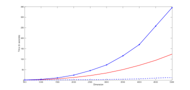
Figure 1. Costs of: $p$ iterations of Metropolized Gibbs sampler (red solid line); 50 iterations of full-VA (blue+ line); and 50 iterations of midsize-VA with $\|\delta^{(\textsf{i})}\|_{0}=100$ (blue-dashed line), as functions of the dimension $p$.

We perform a simulation study to assess the behavior of the posterior distribution and its variational approximations as described in Corollary 5.1. For simplicity we focus on only one of the regression problems. We set $p=1000$, $n\in\{100,500\}$, and we generate $Z=[Y,X]\in\mathbb{R}^{n\times(p+1)}$ as follows. We first generate the matrix $X$ by simulating the rows of $X$ independently from a Gaussian distribution with correlation $\psi^{|j-i|}$ between components $i$ and $j$, where $\psi\in\{0,0.8\}$. When $\psi=0$, the resulting matrix $X$ has a low coherence, but the coherence increases when $\psi=0.8$. Using $X$, we general $Y=X\theta_{\star}+\epsilon/\vartheta_{\star,11}$, with $\vartheta_{\star,11}=1$ that we assume known. We build $\theta_{\star}$ with $s_{\star}=10$ non-zeros components that we fill with draws from the uniform distribution $\pm\mathbf{U}(a,a+1)$, where $a=4\sqrt{s_{\star}\log(p)/n}$.

We build $\Pi$ with $\sigma^{2}=1$, $u=2$, $\rho_{1}=\sqrt{\log(p)/n}$, and $\rho_{0}^{-1}=1/(4n)$. We sample from $\Pi$ using Algorithm 2. We consider two variational approximation. The full-VA, and a mid-size VA with template $\delta^{(\textsf{i})}$ that contains the support of $\theta_{\star}$, and such that $\|\delta^{(\textsf{i})}\|_{0}=100$. We approximate the variational approximations by coordinate ascent variational inference (see e.g. Blei et al. (2017)). The details of these algorithms are given in Appendix C. We initialize all three algorithms from the lasso solution. In Figure 1 we plot the computational cost of the three algorithms as $p$ increases. It shows that the full-VA is actually more expensive than the MCMC sampler. This is due to the need to form the Cholesky decomposition of a large $p\times p$ matrix at each iteration of the full-VA. In contrast, and as explained in Section 2.1 the per-iteration cost of Algorithm 2 is of order $O(s_{\star}p)$. On the other hand, for $p=5,000$ the midsize VA is more than 10 times faster than the MCMC sampler.

Figure 2 shows the (estimated) posterior distributions for the parameters $\theta_{1},\theta_{2}$ and $\theta_{3}$ from one MCMC run of $5,000$ iterations and single CAVI-runs of 50 iterations. Here we are comparing the skinny-VA, and the midsize-VA with $\|\delta^{(\textsf{i})}\|_{0}=100$, for a template $\delta^{(\textsf{i})}$ that contains the support of $\theta_{\star}$. Since we are working in a high signal-to-noise ratio setting the results are fairly consistent across replications. The true signal $\theta_{\star}$ is such that $\theta_{\star,1}\neq 0$ and $\theta_{\star,2}\neq 0$ while $\theta_{\star,3}=0$. Figure 2 shows that as $n$ increases both VA approximations approximate well the quasi-posterior distribution in the low coherence regime. However in presence of correlation, the skinny-VA systematically underestimates the marginal posterior variances when there is correlation between the relevant variables. However, as suggested by Corollary 5.1, the midsize-VA approximates the whole distribution well.

Linear regression with low coherent design matrix. $p=1000$, $n=100$.

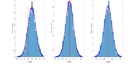
Linear regression with low coherent design matrix. $p=1000$, $n=500$.

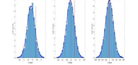
Linear regression with high design matrix . $p=1000$, $n=100$.

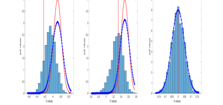
Linear regression with high design matrix. $p=1000$, $n=500$.

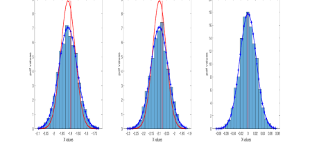
Figure 2. Posterior inference for $\beta_{1}$ (first column), $\beta_{2}$ (second column) and $\beta_{3}$ in the linear regression example based on one MCMC run (histogram), one skinny-VA run (continuous red line), and one midesize-VA run ($+$ blue line). Vertical lines locate the true values of the parameters.

5.2. Sparse principal component estimation

We give another illustration of the quasi-Bayesian framework with a non-standard example from sparse PCA. Principal component analysis is a widely used technique for data exploration and data reduction (Jolliffe (1986)). In order to deal with high-dimensional datasets, several works have introduced recently various versions of PCA that estimate sparse principal components (Jolliffe et al. (2003); Zou et al. (2006); Shen and Huang (2008); Lei and Vu (2015)). Extension of these ideas to a full Bayesian setting has been considered in the literature but is computationally challenging (Pati et al. (2014); Gao and Zhou (2015); Xie et al. (2018)). Using the quasi-Bayesian framework we explore here a fast regression-based approach to sparse PCA that we show works well when the sample size $n$ is close to $p$ and/or the spectral gap is sufficiently large. We consider the following data generating process.

C 1.

The matrix $X\in\mathbb{R}^{n\times p}$ is such that the rows of $X$ are i.i.d. from the Gaussian distribution $\textbf{N}_{p}(0,\Sigma)$ on $\mathbb{R}^{p}$, with a covariance matrix $\Sigma$ of the form

$$\Sigma=\vartheta\theta_{\star}\theta_{\star}^{\prime}+I_{p},$$

for some sparse unit-vector $\theta_{\star}\in\mathbb{R}^{p}$, and some absolute constant $\vartheta>0$. We set $s_{\star}\stackrel{{\scriptstyle\mathrm{def}}}{{=}}\|\theta_{\star}\|_{0}$.

Let $X=U\Lambda V^{\prime}$ be the singular value decomposition (SVD) of $X$. Let $V_{1}$ be the first column of $V$. It was noted by Zou et al. (2006) that setting $y=\Lambda_{11}U_{1}$, it holds for all $\lambda>0$ that

$$V_{1}=\frac{\hat{b}}{\|\hat{b}\|_{2}},\;\;\mbox{ where }\;\;\hat{b}\stackrel{{\scriptstyle\mathrm{def}}}{{=}}\operatorname*{{\mathsf{Argmin}}}_{\beta\in\mathbb{R}^{p}}\|y-X\beta\|_{2}^{2}+\lambda\|\beta\|_{2}^{2}.$$

This result suggests that one can recover the first principal component $V_{1}$ by sparse regression of $y=\Lambda_{11}U_{1}$ on $X$. To implement this idea in a Bayesian framework we are naturally led to the quasi-likelihood function

$$\ell(\theta;X)=-\frac{1}{2\sigma^{2}}\|y-X\theta\|_{2}^{2},\;\;\theta\in\mathbb{R}^{p},$$

for some constant $\sigma^{2}>0$. The resulting quasi-posterior distribution on $\Delta\times\mathbb{R}^{p}$ is the same as in (24):

$$\Pi(\delta,\mathrm{d}\theta|Z)\propto e^{-\frac{1}{2\sigma^{2}}\|y-X\theta_{\delta}\|_{2}^{2}}\omega(\delta)\left(\frac{\rho_{1}}{2\pi}\right)^{\frac{\|\delta\|_{0}}{2}}\left(\frac{\rho_{0}}{2\pi}\right)^{\frac{p-\|\delta\|_{0}}{2}}e^{-\frac{\rho_{1}}{2}\|\theta_{\delta}\|_{2}^{2}}e^{-\frac{\rho_{0}}{2}\|\theta-\theta_{\delta}\|_{2}^{2}}\mathrm{d}\theta.$$

We analyze this quasi-posterior distribution. One challenge here is that we do not possess a good understanding of the distribution of the quasi-score function $X^{\prime}(\Lambda_{11}U_{1}-X\theta_{\star})/\sigma^{2}$ due to the intricate nature of the SVD decomposition. Hence Theorem 1 cannot be applied, and thus we do not know whether the quasi-posterior distribution is automatically sparse under the prior H2. We work around this issue by hard-coding sparsity directly in the prior as follows.

C 2.

We assume that

$$\omega(\delta)\propto\textsf{q}^{\|\delta\|_{0}}(1-\textsf{q})^{p-\|\delta\|_{0}}\textbf{1}_{\Delta_{\bar{s}}}(\delta),\;\;\;\delta\in\Delta,$$

for some integer $\bar{s}\geq s_{\star}$, where $\mathsf{q}\in(0,1)$ is such that $\frac{\mathsf{q}}{1-\mathsf{q}}=\frac{1}{p^{u+1}}$, for some absolute constant $u>0$. Furthermore we will assume that $p\geq 9$, $p^{u/2}\geq 2e^{2\rho}$.

Since $s_{\star}$ is not known, how to find $\bar{s}$ in practice that satisfies $\bar{s}\geq s_{\star}$ is not obvious, and would require some judgment from the researcher. However in terms of computations, using C2 instead of H2 implies only a minor change to the MCMC sampler in Algorithm 2. For $a\in\mathbb{R}$, $\textsf{sign}(a)=1$ if $a\geq 0$, and $-1$ otherwise.

Corollary .

Assume C1, C2, and choose $\sigma^{2}=\vartheta$, $\rho=\sqrt{\log(p)/n}$. Suppose that $\|\theta_{\star}\|_{\infty}=O(1)$, as $p\to\infty$. There exist absolute constants $C_{0},C$ such that for $n\geq C_{0}(\frac{p}{\vartheta}+\bar{s}\log(p))$, we have

$$\lim_{p\to\infty}\mathbb{E}_{\star}\left[\textbf{1}_{\{\textsf{sign}(\left\langle V_{1},\theta_{\star}\right\rangle)=1\}}\Pi\left(\mathsf{B}_{\theta_{\star}}|X\right)+\textbf{1}_{\{\textsf{sign}(\left\langle V_{1},\theta_{\star}\right\rangle)=-1\}}\Pi\left(\mathsf{B}_{-\theta_{\star}}|X\right)\right]=1,$$

where for $\theta_{0}\in\{\theta_{\star},-\theta_{\star}\}$,

$$\mathsf{B}_{\theta_{0}}\stackrel{{\scriptstyle\mathrm{def}}}{{=}}\bigcup_{\delta\in\Delta_{\bar{s}}}\{\delta\}\times\left\{\theta\in\mathbb{R}^{p}:\;\|\theta_{\delta}-\theta_{0}\|_{2}\leq C\vartheta\sqrt{\frac{\left(\frac{p}{\vartheta}+\log(p)\right)(\bar{s}+s_{\star})}{n}},\;\|\theta-\theta_{\delta}\|_{2}\leq 3\sqrt{\gamma p}\right\}.$$

Proof.

See Section A.8. ∎

It is well-known that the principal component is identified only up to a sign, which is reflected in Corollary 5.2. The assumption $\sigma^{2}=\vartheta$ is made for simplicity, since $\vartheta$ is typically unknown. To a certain extent the procedure is robust to a misspecification of $\sigma^{2}$.

The contraction rate suggests that the method would perform poorly if the sample size and the spectral gap are both small, which is confirmed in the simulations. One important limitation of Corollary 5.2 is that the convergence rate does not have the correct dependence on the spectral gap. This is most certainly an artifact of our method of proof.

5.2.1. Numerical illustration

We generate a random matrix $X\in\mathbb{R}^{n\times p}$ according C1 with $p=1000$, and $n\in\{100,1000\}$, where $\beta_{\star}=(0.5,0.5,0,0.5,0.5,0,\ldots,0)^{\prime}$. We consider two levels of the spectral gap $\vartheta\in\{5,20\}$. As above we set up the prior distribution with $u=2$, $\rho_{1}=\sqrt{log(p)/n}$, and $\rho_{0}^{-1}=1/(4n)$. We use the same MCMC sampler as in the Gaussian graphical model of Section 5.1, that we initialize from the lasso solution, and run the $2000$ iterations. We normalize the MCMC output to have unit-norm (at each iteration). We repeat all computations $100$ times and use the replications to approximate the distribution of the posterior means and posterior variances of the first three components of $\theta$ ($\theta_{1},\theta_{2}$ and $\theta_{3}$). Using the $100$ replications we also approximate the distribution of the error

$$\int\left\|\frac{\theta\theta^{\prime}}{\|\theta\|_{2}^{2}}-\theta_{\star}\theta_{\star}^{\prime}\right\|_{2}\Pi(\mathrm{d}\theta|X),$$

that we call projection approximation error. To assess the quasi-likelihood method advocated here we compare its performance to that of the frequentist estimator of (Zou et al. (2006)) as implemented in the Matlab package SpaSM (Sjöstrand et al. (2018)). We present the results on Figure 3 and 4. The results supports very well the conclusions of Corollary 5.2.

Sparse PCA with $\vartheta=5$, $p=1000$, $n=100$.

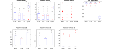
Sparse PCA with $\vartheta=5$, $p=1000$, $n=1000$.

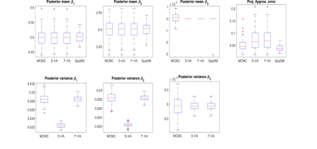
Figure 3. Distributions of posterior means and variances for $\beta_{1},\beta_{2},\beta_{3}$, and distribution of the projection approx. error. Estimated from $100$ replications. S-VA is skinny-VA, F-VA is full-VA. We also report similar distributions for the frequentist estimator computed by SpaSM.

Sparse PCA with $\vartheta=20$, $p=1000$, $n=100$.

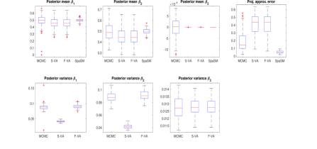
Sparse PCA with $\vartheta=20$, $p=1000$, $n=1000$.

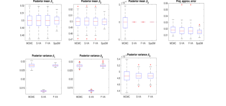
Figure 4. Distributions of posterior means and variances for $\beta_{1},\beta_{2},\beta_{3}$, and distribution of the projection approx. error. Estimated from $100$ replications. S-VA is skinny-VA, F-VA is full-VA. We also report similar distributions for the frequentist estimator computed by SpaSM.

Appendix A Proofs of the main results

A.1. Some preliminary lemmas

Let $\mu_{\delta}(\mathrm{d}\theta)$ denote the product measure on $\mathbb{R}^{p}$ given by

$$\mu_{\delta}(\mathrm{d}\theta)\stackrel{{\scriptstyle\mathrm{def}}}{{=}}\prod_{j=1}^{p}\mu_{\delta_{j}}(\mathrm{d}\theta_{j}),$$

where $\mu_{0}(\mathrm{d}x)$ is the Dirac mass at $0$, and $\mu_{1}(\mathrm{d}x)$ is the Lebesgue measure on $\mathbb{R}$. We start with a useful lower bound on the normalizing constant.

Lemma .

Assume H1-H2. For $z\in\mathcal{Z}$, let $C(z)$ denote the normalizing constant of $\Pi(\cdot|z)$. For $z\in\mathcal{E}_{0}$, we have

$$C(z)\geq\omega(\delta_{\star})e^{\ell(\theta_{\star};z)}e^{-\frac{\rho_{1}}{2}\|\theta_{\star}\|_{2}^{2}}\left(\frac{\rho_{1}}{\bar{\kappa}+\rho_{1}}\right)^{\frac{\|\theta_{\star}\|_{0}}{2}}.$$ (28)

Proof.

The proof is very similar to the proof of Lemma 11 of Atchade (2017). We set

$$\bar{\omega}(\delta)\stackrel{{\scriptstyle\mathrm{def}}}{{=}}\omega(\delta)\left(\frac{\rho_{1}}{2\pi}\right)^{\frac{\|\delta\|_{0}}{2}}\left(\frac{\rho_{0}}{2\pi}\right)^{\frac{p-\|\delta\|_{0}}{2}}.$$

Fix $z\in\mathcal{E}_{0}$. Then $\Pi$ is well-defined, and we have

$$C(z) = \sum_{\delta\in\Delta}\bar{\omega}(\delta)\int_{\mathbb{R}^{p}}e^{-\ell(\theta_{\delta};z)-\frac{\rho_{1}}{2}\|\theta_{\delta}\|_{2}^{2}-\frac{\rho_{0}}{2}\|\theta-\theta_{\delta}\|_{2}^{2}}\mathrm{d}\theta$$

$$\geq \bar{\omega}(\delta_{\star})\int_{\mathbb{R}^{p}}e^{-\ell(\theta_{\delta_{\star}};z)-\frac{\rho_{1}}{2}\|\theta_{\delta_{\star}}\|_{2}^{2}-\frac{\rho_{0}}{2}\|\theta-\theta_{\delta_{\star}}\|_{2}^{2}}\mathrm{d}\theta$$

$$= \bar{\omega}(\delta_{\star})(2\pi\rho_{0}^{-1})^{\frac{p-\|\delta_{\star}\|_{0}}{2}}\int_{\mathbb{R}^{p}}e^{\ell(u;z)-\frac{\rho_{1}}{2}\|u\|_{2}^{2}}\mu_{\delta_{\star}}(\mathrm{d}u).$$

Setting $G\stackrel{{\scriptstyle\mathrm{def}}}{{=}}\nabla\ell(\theta_{\star};z)$, we have for all $u\in\mathbb{R}^{p}_{\delta_{\star}}$ and $z\in\mathcal{E}_{0}$,

$$\ell(u;z)-\ell(\theta_{\star};z)-\left\langle G,u-\theta_{\star}\right\rangle\geq-\frac{\bar{\kappa}}{2}\|u-\theta_{\star}\|_{2}^{2},$$

which implies that

$$C(z)\geq\omega(\delta_{\star})\left(\frac{\rho_{1}}{2\pi}\right)^{s_{\star}/2}e^{\ell(\theta_{\star};z)-\frac{\rho}{2}\|\theta_{\star}\|_{2}^{2}}\int_{\mathbb{R}^{p}}e^{\left\langle G,u-\theta_{\star}\right\rangle-\frac{\bar{\kappa}}{2}\|u-\theta_{\star}\|_{2}^{2}+\frac{\rho_{1}}{2}\|\theta_{\star}\|_{2}^{2}-\frac{\rho_{1}}{2}\|u\|_{2}^{2}}\mu_{\delta_{\star}}(\mathrm{d}u).$$

For all $u\in\mathbb{R}^{p}_{\delta_{\star}}$, $(1/2)(\|\theta_{\star}\|_{2}^{2}-\|u\|_{2}^{2})=-\frac{1}{2}\|u-\theta_{\star}\|_{2}^{2}-\left\langle\theta_{\star},u-\theta_{\star}\right\rangle$. Therefore,

$$\int_{\mathbb{R}^{p}}e^{\left\langle G,u-\theta_{\star}\right\rangle-\frac{\bar{\kappa}}{2}\|u-\theta_{\star}\|_{2}^{2}+\frac{\rho_{1}}{2}\|\theta_{\star}\|_{2}^{2}-\frac{\rho_{1}}{2}\|u\|_{2}^{2}}\mu_{\delta_{\star}}(\mathrm{d}u)\\ =\int_{\mathbb{R}^{p}}e^{\left\langle G-\rho_{1}\theta_{\star},u-\theta_{\star}\right\rangle-\frac{\bar{\kappa}+\rho_{1}}{2}\|u-\theta_{\star}\|_{2}^{2}}\mu_{\delta_{\star}}(\mathrm{d}u)=\left(\frac{2\pi}{\bar{\kappa}+\rho_{1}}\right)^{\frac{s_{\star}}{2}}e^{\frac{\bar{\kappa}+\rho_{1}}{2}\|G-\rho_{1}\theta_{\star}\|_{2}^{2}},$$

and (28) follows easily.

∎

Our proofs rely on the existence of some generalized testing procedures that we develop next, following ideas from Atchade (2017). More specifically we will make use of the following result which follows by combining Lemma 6.1 and Equation (6.1) of Kleijn and van der Vaart (2006).

Lemma (Kleijn-Van der Vaart (2006)).

Let $(\mathcal{X},\mathcal{B},\lambda)$ be a measure space with a sigma-finite measure $\lambda$. Let $p$ be a density on $\mathcal{X}$, and $\mathcal{Q}$ a family of integrable real-valued functions on $\mathcal{X}$. There exists a measurable $\phi:\;\mathcal{X}\to[0,1]$ such that

$$\sup_{q\in\mathcal{Q}}\left[\int\phi p\mathrm{d}\lambda+\int(1-\phi)q\mathrm{d}\lambda\right]\leq\sup_{q\in\textsf{conv}(\mathcal{Q})}\mathcal{H}(p,q),$$

where $\textsf{conv}(\mathcal{Q})$ is the convex hull of $\mathcal{Q}$, and $\mathcal{H}(q_{1},q_{2})\stackrel{{\scriptstyle\mathrm{def}}}{{=}}\int\sqrt{q_{1}q_{2}}\mathrm{d}\lambda$.

We introduce the quasi-likelihood

$$f_{\theta}(z)\stackrel{{\scriptstyle\mathrm{def}}}{{=}}e^{\ell(\theta;z)},\;\;\theta\in\mathbb{R}^{p},\;z\in\mathcal{Z}.$$

For $\theta_{1}\in\mathbb{R}^{p}$, we recall that

$$\mathcal{L}_{\theta_{1}}(\theta;z)\stackrel{{\scriptstyle\mathrm{def}}}{{=}}\ell(\theta;z)-\ell(\theta_{1};z)-\left\langle\nabla\ell(\theta_{1};z),\theta-\theta_{1}\right\rangle,\;\theta\in\mathbb{R}^{p}.$$

We develop the test in a slightly more general setting. More specifically , in order to handle the PCA example we will allow the mode of $\ell(\cdot;z)$ to depend on $z$.

Let $\delta_{\star}$ be some sparse element $\Delta$. Let $\Theta_{\star}$ be a finite nonempty subset of $\mathbb{R}^{p}_{\delta_{\star}}$ (the set of possible contraction points). Let $\bar{\rho}>0$ be a constant, $\bar{s}\geq 1$ an integer, and r a rate function. For each $\theta_{\star}\in\Theta_{\star}$, we define

$$\mathcal{E}_{\textsf{t},\theta_{\star}}\stackrel{{\scriptstyle\mathrm{def}}}{{=}}\left\{z\in\mathcal{Z}:\;\|\nabla\log f_{\theta_{\star}}(z)\|_{\infty}\leq\frac{\bar{\rho}}{2},\;\;\right.\\ \left.\mbox{ and for all }\delta\in\Delta_{\bar{s}},\;\theta\in\mathbb{R}^{p}_{\delta},\;\mathcal{L}_{\theta_{\star}}(\theta;z)\leq-\frac{1}{2}\textsf{r}(\|\theta-\theta_{\star}\|_{2})\right\},$$

which roughly represents the set of data points for which $\Pi(\cdot|z)$ could contract towards $\theta_{\star}$.

Lemma .

Set $s_{\star}\stackrel{{\scriptstyle\mathrm{def}}}{{=}}\|\delta_{\star}\|_{0}$, and

$$\epsilon\stackrel{{\scriptstyle\mathrm{def}}}{{=}}\inf\left\{z>0:\;\textsf{r}(x)-2\bar{\rho}(s_{\star}+\bar{s})^{1/2}x\geq 0,\;\mbox{ for all }x\geq z\right\}.$$

Let $f_{\star}$ be a density on $\mathcal{Z}$, and $M>2$ a constant. There exists a measurable function $\phi:\mathcal{Z}\to[0,1]$ such that

$$\int_{\mathcal{Z}}\phi(z)f_{\star}(z)\mathrm{d}z\leq\frac{2|\Theta_{\star}|(9p)^{\bar{s}}e^{-\frac{M}{8}\bar{\rho}(s_{\star}+\bar{s})^{1/2}\epsilon}}{1-e^{-\frac{M}{8}\bar{\rho}(s_{\star}+\bar{s})^{1/2}\epsilon}},$$

where $|\Theta_{\star}|$ denotes the cardinality of $\Theta_{\star}$. Furthermore, for any $\delta\in\Delta_{\bar{s}}$, any $\theta\in\mathbb{R}^{p}_{\delta}$ such that $\|\theta-\theta_{\star}\|_{2}>jM\epsilon$ for some $j\geq 1$, and some $\theta_{\star}\in\Theta_{\star}$, we have

$$\int_{\mathcal{E}_{\textsf{t},\theta_{\star}}}(1-\phi(z))\frac{f_{\theta}(z)}{f_{\theta_{\star}}(z)}f_{\star}(z)\mathrm{d}z\leq e^{-\frac{1}{8}\textsf{r}\left(\frac{jM\epsilon}{2}\right)}.$$

Proof.

Define

$$\bar{q}_{\theta_{\star},u}(z)\stackrel{{\scriptstyle\mathrm{def}}}{{=}}\frac{f_{u}(z)}{f_{\theta_{\star}}(z)}f_{\star}(z)\textbf{1}_{\mathcal{E}_{\textsf{t},\theta_{\star}}}(z),\;\;\;\theta_{\star}\in\Theta_{\star},\;\;u\in\mathbb{R}^{p},\;\;z\in\mathcal{Z}.$$

Using the properties of the event $\mathcal{E}_{\textsf{t},\theta_{\star}}$, we note that for $\delta\in\Delta_{\bar{s}}$, and $u\in\mathbb{R}^{p}_{\delta}$ we have

$$\int_{\mathcal{Z}}\bar{q}_{\theta_{\star},u}(z)\mathrm{d}z=\int_{\mathcal{E}_{\textsf{t},\theta_{\star}}}e^{\left\langle\nabla\ell(\theta_{\star};z),u-\theta_{\star}\right\rangle+\mathcal{L}_{\theta_{\star}}(u;z)}f_{\star}(z)\mathrm{d}z\leq e^{\frac{\bar{\rho}}{2}\|u-\theta_{\star}\|_{1}}<\infty.$$ (29)

Fix $\eta\geq 2\epsilon$ arbitrary. Fix $\theta_{\star}\in\Theta_{\star}$, $\delta\in\Delta_{\bar{s}}$, and fix $\theta\in\mathbb{R}^{p}_{\delta}$ such that $\|\theta-\theta_{\star}\|_{2}>\eta$. Let

$$\mathcal{P}=\mathcal{P}_{\theta_{\star},\delta,\theta}\stackrel{{\scriptstyle\mathrm{def}}}{{=}}\left\{\bar{q}_{\theta_{\star},u}:\;u\in\mathbb{R}^{p}_{\delta},\;\|u-\theta\|_{2}\leq\frac{\eta}{2}\right\}.$$

According to Lemma A.1, applied with $p=f_{\star}$, and $\mathcal{Q}=\mathcal{P}$, there exists a test function $\phi_{\theta_{\star},\delta,\theta}$ (that we will write simply as $\phi$ for convenience) such that

$$\sup_{q\in\mathcal{P}}\left[\int\phi f_{\star}+\int(1-\phi)q\right]\leq\sup_{q\in\textsf{conv}(\mathcal{P})}\int_{\mathcal{Z}}\sqrt{f_{\star}(z)q(z)}\mathrm{d}z.$$ (30)

Any $q\in\textsf{conv}(\mathcal{P})$ can be written as $q=\sum_{j}\alpha_{j}\bar{q}_{\theta_{\star},u_{j}}$, where $\sum_{j}\alpha_{j}=1$, $u_{j}\in\mathbb{R}^{p}_{\delta}$, $\|u_{j}-\theta\|_{2}\leq\eta/2$. Notice that this implies that $\|u_{j}-\theta_{\star}\|_{2}>\eta/2\geq\epsilon$. Therefore, by Jensen’s inequality, the first inequality of (29), and the properties of the set $\mathcal{E}_{\textsf{t},\theta_{\star}}$, we get

$$\int_{\mathcal{Z}}\sqrt{f_{\star}(z)q(z)}\mathrm{d}z \leq \sqrt{\sum_{j}\alpha_{j}\int_{\mathcal{E}_{\textsf{t},\theta_{\star}}}\frac{f_{u_{j}}(z)}{f_{\theta_{\star}}(z)}f_{\star}(z)\mathrm{d}z}$$

$$\leq \sqrt{\sum_{j}\alpha_{j}e^{\frac{\bar{\rho}}{2}\|u_{j}-\theta_{\star}\|_{1}-\frac{1}{2}\textsf{r}(\|u_{j}-\theta_{\star}\|_{2})}},$$

$$\leq \sqrt{\sum_{j}\alpha_{j}e^{-\frac{1}{4}\textsf{r}(\|u_{j}-\theta_{\star}\|_{2})}}$$

$$\leq e^{-\frac{1}{8}\textsf{r}\left(\frac{\eta}{2}\right)}.$$

Consequently, (30) yields

$$\sup_{q\in\mathcal{P}}\left[\int\phi f_{\star}+\int(1-\phi)q\right]\leq e^{-\frac{1}{8}\textsf{r}\left(\frac{\eta}{2}\right)}.$$ (31)

For $M>2$, write $\cup_{\theta_{\star}}\cup_{\delta}\{\theta\in\mathbb{R}^{p}_{\delta}:\;\|\theta-\theta_{\star}\|_{2}>M\epsilon\}$ as $\cup_{\theta_{\star}}\cup_{\delta}\cup_{j\geq 1}\mathcal{A}_{\epsilon}(\theta_{\star},\delta,j)$, where the unions in $\delta$ are taken over all $\delta$ such that $\|\delta\|_{0}\leq\bar{s}$, and

$$\mathcal{A}_{\epsilon}(\theta_{\star},\delta,j)\stackrel{{\scriptstyle\mathrm{def}}}{{=}}\left\{\theta\in\mathbb{R}^{p}_{\delta}:\;jM\epsilon<\|\theta-\theta_{\star}\|_{2}\leq(j+1)M\epsilon\right\}.$$

For $\mathcal{A}_{\epsilon}(\theta_{\star},\delta,j)\neq\emptyset$, let $\mathcal{S}(\theta_{\star},\delta,j)$ be a maximally $(jM\epsilon/2)$-separated point in $\mathcal{A}_{\epsilon}(\theta_{\star},\delta,j)$. It is easily checked that the cardinality of $\mathcal{S}(\theta_{\star},\delta,j)$ is upper bounded by $9^{\|\delta\|_{0}}\leq 9^{\bar{s}}$ (see for instance Ghosal et al. (2000) Example 7.1 for the arguments). For $\theta\in\mathcal{S}(\theta_{\star},\delta,j)$, let $\phi$ denote the test function obtained above with $\eta=jM\epsilon$. From (31), this test satisfies

$$\sup_{u\in\mathbb{R}^{p}_{\delta},\;\|u-\theta\|_{2}\leq\frac{jM\epsilon}{2}}\left[\int_{\mathcal{Z}}\phi(z)f_{\star}(z)\mathrm{d}z+\int_{\mathcal{Z}}(1-\phi(z))\bar{q}_{\theta_{\star},u}(z)\mathrm{d}z\right]\leq e^{-\frac{1}{8}\textsf{r}\left(\frac{jM\epsilon}{2}\right)}.$$ (32)

We then set

$$\bar{\phi}=\max_{\theta_{\star}\in\Theta_{\star}}\;\max_{\delta:\;\|\delta\|_{0}\leq\bar{s}}\;\;\sup_{j\geq 1}\;\max_{\theta\in\mathcal{S}(\theta_{\star},\delta,j)}\;\phi.$$

It then follows that

$$\int_{\mathcal{Z}}\bar{\phi}(z)f_{\star}(z)\mathrm{d}z\leq\sum_{\theta_{\star}}\sum_{k=0}^{\bar{s}}\;\sum_{\delta:\;\|\delta\|_{0}=k}\;\sum_{j\geq 1}\;\sum_{\theta\in\mathcal{S}(\theta_{\star},\delta,j)}\int_{\mathcal{Z}}\phi(z)f_{\star}(z)\mathrm{d}z\\ \leq|\Theta_{\star}|\sum_{k=0}^{\bar{s}}{p\choose k}9^{k}\sum_{j\geq 1}e^{-\frac{1}{8}\textsf{r}\left(\frac{jM\epsilon}{2}\right)}\leq 2|\Theta_{\star}|(9p)^{\bar{s}}\sum_{j\geq 1}e^{-\frac{1}{8}\textsf{r}\left(\frac{jM\epsilon}{2}\right)}.$$

Since $jM\epsilon/2\geq\epsilon$, we can say that $\textsf{r}(jM\epsilon/2)\geq 2\bar{\rho}(s_{\star}+\bar{s})^{1/2}(jM\epsilon/2)$. Hence

$$\sum_{j\geq 1}e^{-\frac{1}{8}\textsf{r}\left(\frac{jM\epsilon}{2}\right)}\leq\frac{e^{-\frac{M}{8}\bar{\rho}(s_{\star}+\bar{s})^{1/2}\epsilon}}{1-e^{-\frac{M}{8}\bar{\rho}(s_{\star}+\bar{s})^{1/2}\epsilon}}.$$

And if for some $\delta$, such that $\|\delta\|_{0}\leq\bar{s}$, some $\theta_{\star}\in\Theta_{\star}$, and some $\theta\in\mathbb{R}^{p}_{\delta}$ we have $\|\theta-\theta_{\star}\|_{2}>jM\epsilon$, then $\theta$ resides within $(iM\epsilon)/2$ of some point $\theta_{0}\in\mathcal{S}(\theta_{\star},\delta,i)$ for some $i\geq j$. Hence, by (32),

$$\int_{\mathcal{Z}}(1-\bar{\phi}(z))\bar{q}_{\theta_{\star},\theta}(z)\mathrm{d}z\leq\int_{\mathcal{Z}}(1-\phi(z))\bar{q}_{\theta_{\star},\theta}(z)\mathrm{d}z\leq e^{-\frac{1}{8}\textsf{r}\left(\frac{iM\epsilon}{2}\right)}\leq e^{-\frac{1}{8}\textsf{r}\left(\frac{jM\epsilon}{2}\right)}.$$

This ends the proof. ∎

A.2. Proof Theorem 1

Let $f:\;\Delta\times\mathbb{R}^{p}\to[0,\infty)$ be some arbitrary measurable function. Take $\mathcal{E}\subseteq\mathcal{E}_{0}$. By the control on the normalizing constant obtained in Lemma A.1, we have

$$\textbf{1}_{\mathcal{E}}(z)\int f\mathrm{d}\Pi(\cdot|z)\leq\left(1+\frac{\bar{\kappa}}{\rho_{1}}\right)^{\frac{s_{\star}}{2}}\\ \times\sum_{\delta\in\Delta}\;\frac{\omega(\delta)}{\omega(\delta_{\star})}\left(\frac{\rho_{1}}{2\pi}\right)^{\frac{\|\delta\|_{0}}{2}}\textbf{1}_{\mathcal{E}}(z)\int_{\mathbb{R}^{p}}f(\delta,u)\frac{e^{\ell(u;z)-\frac{\rho_{1}}{2}\|u\|_{2}^{2}}}{e^{\ell(\theta_{\star};z)-\frac{\rho_{1}}{2}\|\theta_{\star}\|_{2}^{2}}}\mu_{\delta}(\mathrm{d}u).$$

We write

$$\ell(u;z)-\ell(\theta_{\star};z)=\mathcal{L}_{\theta_{\star}}(u;z)+\left\langle\nabla\ell(\theta_{\star};z),u-\theta_{\star}\right\rangle.$$

Therefore, since for $z\in\mathcal{E}\subseteq\mathcal{E}_{0}$, $\|\nabla\ell(\theta_{\star};z)\|_{\infty}\leq\bar{\rho}/2$, it follows that for $z\in\mathcal{E}$

$$\ell(u;z)-\ell(\theta_{\star};z)\leq\mathcal{L}_{\theta_{\star}}(u;z)+\left(1-\frac{\rho_{1}}{\bar{\rho}}\right)\left\langle\nabla\ell(\theta_{\star};z),u-\theta_{\star}\right\rangle+\frac{\rho_{1}}{2}\|u-\theta_{\star}\|_{1}.$$

We deduce from the above and Fubini’s theorem that

$$\mathbb{E}_{\star}\left[\textbf{1}_{\mathcal{E}}(Z)\int f\mathrm{d}\Pi(\cdot|Z)\right]\leq\left(1+\frac{\bar{\kappa}}{\rho_{1}}\right)^{\frac{s_{\star}}{2}}\sum_{\delta\in\Delta}\;\frac{\omega(\delta)}{\omega(\delta_{\star})}\left(\frac{\rho_{1}}{2\pi}\right)^{\frac{\|\delta\|_{0}}{2}}\\ \times\int_{\mathbb{R}^{p}}f(\delta,u)e^{\frac{\rho_{1}}{2}\left(\|\theta_{\star}\|_{2}^{2}-\|u\|_{2}^{2}\right)+\frac{\rho_{1}}{2}\|u-\theta_{\star}\|_{1}}\mathbb{E}_{\star}\left[\textbf{1}_{\mathcal{E}}(Z)e^{\mathcal{L}(u;Z)+\left(1-\frac{\rho_{1}}{\bar{\rho}}\right)\left\langle\nabla\ell(\theta_{\star};Z),u-\theta_{\star}\right\rangle}\right]\mu_{\delta}(\mathrm{d}u).$$ (33)

Set $\textsf{d}(u)\stackrel{{\scriptstyle\mathrm{def}}}{{=}}-\rho_{1}\|u\|_{1}+\rho_{1}\|\theta_{\star}\|_{1}+(\rho_{1}/2)\|u-\theta_{\star}\|_{1}$, $u\in\mathbb{R}^{p}$. Given (2), we claim that

$$e^{\textsf{d}(u)}\mathbb{E}_{\star}\left[\textbf{1}_{\mathcal{E}}(Z)e^{\mathcal{L}(u;Z)+\left(1-\frac{\rho_{1}}{\bar{\rho}}\right)\left\langle\nabla\ell(\theta_{\star};Z),u-\theta_{\star}\right\rangle}\right]\leq e^{\frac{\mathsf{a}_{0}}{2}}e^{-\frac{\rho_{1}}{4}\|u-\theta_{\star}\|_{1}},\;\;\;u\in\mathbb{R}^{p},$$ (34)

where $\mathsf{a}_{0}=-\min_{x>0}[\textsf{r}_{0}(x)-4\rho_{1}s_{\star}^{1/2}]$. The proof of this statement is essentially the same as in Castillo et al. (2015) Theorem 1. We give the details for completeness. Indeed,

$$\textsf{d}(u) = \frac{\rho_{1}}{2}\|\delta_{\star}\cdot(u-\theta_{\star})\|_{1}+\frac{\rho_{1}}{2}\|\delta_{\star}^{c}\cdot u\|_{1}-\rho_{1}\|\delta_{\star}\cdot u\|_{1}-\rho_{1}\|\delta_{\star}^{c}\cdot u\|_{1}+\rho_{1}\|\theta_{\star}\|_{1}$$

$$\leq -\frac{\rho_{1}}{2}\|\delta_{\star}^{c}\cdot(u-\theta_{\star})\|_{1}+\frac{3\rho_{1}}{2}\|\delta_{\star}\cdot(u-\theta_{\star})\|_{1}.$$

If $\|\delta_{\star}^{c}\cdot(u-\theta_{\star})\|_{1}>7\|\delta_{\star}\cdot(u-\theta_{\star})\|_{1}$, we easily deduce that $\textsf{d}(u)\leq-\frac{\rho_{1}}{4}\|u-\theta_{\star}\|_{1}$. This bound together with (2) shows that the claim holds true when $\|\delta_{\star}^{c}\cdot(u-\theta_{\star})\|_{1}>7\|\delta_{\star}\cdot(u-\theta_{\star})\|_{1}$. If $\|\delta_{\star}^{c}\cdot(u-\theta_{\star})\|_{1}\leq 7\|\delta_{\star}\cdot(u-\theta_{\star})\|_{1}$, then again by (2), and the bound on $\textsf{d}(u)$ obtained above, we deduce that the logarithm of the left-hand side of (34) is upper bounded by

$$-\frac{\rho_{1}}{2}\|\delta_{\star}^{c}\cdot(u-\theta_{\star})\|_{1}+\frac{3\rho_{1}}{2}\|\delta_{\star}\cdot(u-\theta_{\star})\|_{1}-\frac{1}{2}\textsf{r}_{0}(\|\delta_{\star}\cdot(u-\theta_{\star})\|_{2})\\ \leq-\frac{\rho_{1}}{2}\|u-\theta_{\star}\|_{1}+2\rho_{1}s_{\star}^{1/2}\|\delta_{\star}\cdot(u-\theta_{\star})\|_{2}-\frac{1}{2}\textsf{r}_{0}(\|\delta_{\star}\cdot(u-\theta_{\star})\|_{2})\\ \leq-\frac{\rho_{1}}{2}\|u-\theta_{\star}\|_{1}-\frac{1}{2}\left[\textsf{r}_{0}(\|\delta_{\star}\cdot(u-\theta_{\star})\|_{2})-4\rho_{1}s_{\star}^{1/2}\|\delta_{\star}\cdot(u-\theta_{\star})\|_{2}\right]\\ \leq-\frac{\rho_{1}}{2}\|u-\theta_{\star}\|_{1}+\frac{\mathsf{a_{0}}}{2},$$

which also gives the stated claim. Hence (33) becomes

$$\mathbb{E}_{\star}\left[\textbf{1}_{\mathcal{E}}(Z)\int f\mathrm{d}\Pi(\cdot|Z)\right]\leq\left(1+\frac{\bar{\kappa}}{\rho_{1}}\right)^{\frac{s_{\star}}{2}}e^{\frac{\mathsf{a_{0}}}{2}}\sum_{\delta\in\Delta}\;\frac{\omega(\delta)}{\omega(\delta_{\star})}\left(\frac{\rho_{1}}{2\pi}\right)^{\frac{\|\delta\|_{0}}{2}}\\ \times\int_{\mathbb{R}^{p}}f(\delta,u)e^{\frac{\rho_{1}}{2}\left(\|\theta_{\star}\|_{2}^{2}-\|u\|_{2}^{2}\right)-\rho_{1}\left(\|\theta_{\star}\|_{1}-\|u\|_{1}\right)}e^{-\frac{\rho_{1}}{4}\|u-\theta_{\star}\|_{1}}\mu_{\delta}(\mathrm{d}u).$$ (35)

The integral in the last display is bounded from above by

$$\int_{\mathbb{R}^{p}}f(\delta,u)e^{-\frac{\rho_{1}}{2}\|u-\theta_{\star}\|_{2}^{2}+\rho_{1}\|\theta_{\star}\|_{2}\|u-\theta_{\star}\|_{2}+\frac{3\rho_{1}}{4}\|u-\theta_{\star}\|_{1}}\mu_{\delta}(\mathrm{d}u)\\ \leq e^{2\rho_{1}\|\theta_{\star}\|_{2}^{2}}e^{2\rho_{1}\|\delta\|_{0}}\int_{\mathbb{R}^{p}}f(\delta,u)e^{-\frac{\rho_{1}}{4}\|u-\theta_{\star}\|_{2}^{2}}\mu_{\delta}(\mathrm{d}u),$$

using some simple algebraic majoration. Then (35) becomes

$$\mathbb{E}_{\star}\left[\textbf{1}_{\mathcal{E}}(Z)\int f\mathrm{d}\Pi(\cdot|Z)\right]\leq\left(1+\frac{\bar{\kappa}}{\rho_{1}}\right)^{\frac{s_{\star}}{2}}e^{\frac{\mathsf{a_{0}}}{2}+2\rho_{1}\|\theta_{\star}\|_{2}^{2}}\\ \times\sum_{\delta\in\Delta}\;\frac{\omega(\delta)}{\omega(\delta_{\star})}(\sqrt{2}e^{2\rho_{1}})^{\|\delta\|_{0}}\left(\frac{\rho_{1}}{4\pi}\right)^{\frac{\|\delta\|_{0}}{2}}\int_{\mathbb{R}^{p}}f(\delta,u)e^{-\frac{\rho_{1}}{4}\|u-\theta_{\star}\|_{2}^{2}}\mu_{\delta}(\mathrm{d}u).$$ (36)

In the special case where $f(\delta,u)=\textbf{1}_{\{\|\delta\|_{0}\geq s_{\star}+k\}}$ for some $k\geq 0$, we have

$$\mathbb{E}_{\star}\left[\textbf{1}_{\mathcal{E}}(Z)\Pi(\|\delta\|_{0}\geq s_{\star}+k|Z)\right]\leq\left(1+\frac{\bar{\kappa}}{\rho_{1}}\right)^{\frac{s_{\star}}{2}}e^{\frac{\mathsf{a_{0}}}{2}+2\rho_{1}\|\theta_{\star}\|_{2}^{2}}\sum_{\delta:\;\|\delta\|_{0}\geq s_{\star}+k}\frac{\omega(\delta)}{\omega_{\delta_{\star}}}\left(\sqrt{2}e^{2\rho_{1}}\right)^{\|\delta\|_{0}}.$$

By H2, we have

$$\sum_{\delta:\;\|\delta\|_{0}\geq s_{\star}+k}\frac{\omega(\delta)}{\omega(\delta_{\star})}\left(\sqrt{2}e^{2\rho_{1}}\right)^{\|\delta\|_{0}}=\sum_{j=s_{\star}+k}^{p}{p\choose j}\left(\frac{\textsf{q}}{1-\textsf{q}}\right)^{j-s_{\star}}\left(\sqrt{2}e^{2\rho_{1}}\right)^{j}\\ \leq{p\choose s_{\star}}\left(\sqrt{2}e^{2\rho_{1}}\right)^{s_{\star}}\sum_{j=s_{\star}+k}^{p}\left(\frac{\sqrt{2}e^{2\rho_{1}}}{p^{u}}\right)^{j-s_{\star}},$$

using the fact that $\frac{\textsf{q}}{1-\textsf{q}}=\frac{1}{p^{u+1}}$, and ${p\choose j}\leq p^{j-s_{\star}}{p\choose s_{\star}}$. Hence for $p^{u/2}\geq 2e^{2\rho_{1}}$ we get

$$\sum_{\delta:\;\|\delta\|_{0}\geq s_{\star}+k}\frac{\omega(\delta)}{\omega(\delta_{\star})}\left(\sqrt{2}e^{2\rho_{1}}\right)^{\|\delta\|_{0}}\leq 2{p\choose s_{\star}}\left(\sqrt{2}e^{2\rho_{1}}\right)^{s_{\star}}\frac{1}{p^{\frac{uk}{2}}}\leq 2e^{s_{\star}(\frac{1}{2}+2\rho_{1})+s_{\star}\log(p)-\frac{uk}{2}\log(p)}.$$

Hence we conclude that

$$\mathbb{E}_{\star}\left[\textbf{1}_{\mathcal{E}}(Z)\Pi(\|\delta\|_{0}\geq s_{\star}+k|Z)\right]\\ \leq 2e^{s_{\star}\left(\frac{1}{2}+2\rho_{1}+\log(p)\right)+\frac{s_{\star}}{2}\log\left(1+\frac{\bar{\kappa}}{\rho_{1}}\right)}e^{\frac{\mathsf{a_{0}}}{2}+2\rho_{1}\|\theta_{\star}\|_{2}^{2}}e^{-\frac{uk}{2}\log(p)}\\ \leq 2e^{(1+c_{0})s_{\star}\log(p)}e^{-\frac{uk}{2}\log(p)},$$

using (3). Setting $k=(2/u)(1+c_{0})s_{\star}+j$ for some $j\geq 1$ yields the stated result. This completes the proof.

$\square$

A.3. Proof of Theorem 2

We write $\mathcal{E}_{1}$ instead of $\mathcal{E}_{1}(\bar{s})$, and take $\mathcal{E}\subseteq\mathcal{E}_{1}$. We note that $\mathsf{B}^{c}=\{\delta\in\Delta:\;\|\delta\|_{0}>\bar{s}\}\cup\mathcal{F}_{1}\cup\mathcal{F}_{2}$, where

$$\mathcal{F}_{1}\stackrel{{\scriptstyle\mathrm{def}}}{{=}}\bigcup_{\delta\in\Delta_{\bar{s}}}\{\delta\}\times\left\{\theta\in\mathbb{R}^{p}:\;\|\theta_{\delta}-\theta_{\star}\|_{2}>C\epsilon\right\},$$

$$\;\;\;\mathcal{F}_{2}\stackrel{{\scriptstyle\mathrm{def}}}{{=}}\bigcup_{\delta\in\Delta_{\bar{s}}}\{\delta\}\times\left\{\theta\in\mathbb{R}^{p}:\;\|\theta_{\delta}-\theta_{\star}\|_{2}\leq C\epsilon,\;\;\mbox{ and }\;\;\|\theta-\theta_{\delta}\|_{2}>\epsilon_{1}\right\},$$

where $\epsilon_{1}=\sqrt{(1+C_{1})\rho_{0}^{-1}p}$. Therefore we have

$$\textbf{1}_{\mathcal{E}}(Z)\Pi(\mathsf{B}^{c}|Z)=\textbf{1}_{\mathcal{E}}(Z)\Pi(\|\delta\|_{0}>\bar{s}|Z)+\textbf{1}_{\mathcal{E}}(Z)\Pi(\mathcal{F}_{1}|Z)+\textbf{1}_{\mathcal{E}}(Z)\Pi(\mathcal{F}_{2}|Z).$$ (37)

Let $\phi$ denote the test function asserted by Lemma A.1 with $M\leftarrow C$, $\Theta_{\star}=\{\theta_{\star}\}$. We can then write

$$\mathbb{E}_{\star}\left[\textbf{1}_{\mathcal{E}}(Z)\Pi(\mathcal{F}_{1}|Z)\right]\leq\mathbb{E}_{\star}\left(\phi(Z)\right)+\mathbb{E}_{\star}\left[\textbf{1}_{\mathcal{E}}(Z)\left(1-\phi(Z)\right)\Pi(\mathcal{F}_{1}|Z)\right].$$ (38)

Lemma A.1 gives

$$\mathbb{E}_{\star}\left(\phi(Z)\right)\leq\frac{2(9p)^{\bar{s}}e^{-\frac{C}{8}\bar{\rho}_{1}(s_{\star}+\bar{s})^{1/2}\epsilon}}{1-e^{-\frac{C}{8}\bar{\rho}_{1}(s_{\star}+\bar{s})^{1/2}\epsilon}}\leq 4e^{-\frac{C}{32}\bar{\rho}_{1}(s_{\star}+\bar{s})^{1/2}\epsilon},$$ (39)

for $(C/16)\bar{\rho}(\bar{s}+s_{\star})^{1/2}\epsilon\geq 2\bar{s}\log(p)$. By Lemma A.1, we have

$$\textbf{1}_{\mathcal{E}}(Z)\Pi(\mathcal{F}_{1}|Z) \leq \textbf{1}_{\mathcal{E}}(Z)\left(1+\frac{\bar{\kappa}}{\rho_{1}}\right)^{s_{\star}/2}$$

$$\times\sum_{\delta\in\Delta_{\bar{s}}}\frac{\omega(\delta)}{\omega(\delta_{\star})}\left(\frac{\rho_{1}}{2\pi}\right)^{\|\delta\|_{0}/2}\int_{\mathcal{F}_{\epsilon}^{(\delta)}}\frac{e^{\ell(\theta;Z)-\frac{\rho_{1}}{2}\|\theta\|_{2}^{2}}}{e^{\ell(\theta_{\star};Z)-\frac{\rho_{1}}{2}\|\theta_{\star}\|_{2}^{2}}}\mu_{\delta}(\mathrm{d}\theta),$$

where $\mathcal{F}_{\epsilon}^{(\delta)}\stackrel{{\scriptstyle\mathrm{def}}}{{=}}\{\theta\in\mathbb{R}^{p}:\;\|\theta_{\delta}-\theta_{\star}\|_{2}>C\epsilon\}$. We use this last display together with Fubini’s theorem, to conclude that

$$\mathbb{E}_{\star}\left[\textbf{1}_{\mathcal{E}}(Z)\left(1-\phi(Z)\right)\Pi(\mathcal{F}_{1}|Z)\right]\\ \left(1+\frac{\bar{\kappa}}{\rho_{1}}\right)^{s_{\star}/2}\sum_{\delta\in\Delta_{\bar{s}}}\frac{\omega(\delta)}{\omega(\delta_{\star})}\left(\frac{\rho_{1}}{2\pi}\right)^{\|\delta\|_{0}/2}\\ \times\int_{\mathcal{F}_{\epsilon}^{(\delta)}}\mathbb{E}_{\star}\left[(1-\phi(Z))\frac{e^{\ell(\theta;Z)}}{e^{\ell(\theta_{\star};Z)}}\textbf{1}_{\mathcal{E}}(Z)\right]\frac{e^{-\frac{\rho_{1}}{2}\|\theta\|_{2}^{2}}}{e^{-\frac{\rho_{1}}{2}\|\theta_{\star}\|_{2}^{2}}}\mu_{\delta}(\mathrm{d}\theta).$$ (40)

We write $\mathcal{F}_{\epsilon}^{(\delta)}=\cup_{j\geq 1}\mathcal{F}^{(\delta)}_{j,\epsilon}$, where $\mathcal{F}_{j,\epsilon}^{(\delta)}\stackrel{{\scriptstyle\mathrm{def}}}{{=}}\{\theta\in\mathbb{R}^{p}:\;jC\epsilon<\|\theta_{\delta}-\theta_{\star}\|_{2}\leq(j+1)C\epsilon\}$. Using this and Lemma A.1, we have

$$\int_{\mathcal{F}_{j,\epsilon}^{(\delta)}}\mathbb{E}_{\star}\left[(1-\phi(Z))\frac{e^{\ell(\theta;Z)}}{e^{\ell(\theta_{\star};Z)}}\textbf{1}_{\mathcal{E}}(Z)\right]\frac{e^{-\frac{\rho_{1}}{2}\|\theta\|_{2}^{2}}}{e^{-\frac{\rho_{1}}{2}\|\theta_{\star}\|_{2}^{2}}}\mu_{\delta}(\mathrm{d}\theta)\\ \leq e^{-\frac{1}{8}\textsf{r}\left(\frac{jC\epsilon}{2}\right)}\int_{\mathcal{F}_{j,\epsilon}^{(\delta)}}\frac{e^{-\frac{\rho_{1}}{2}\|\theta\|_{2}^{2}}}{e^{-\frac{\rho_{1}}{2}\|\theta_{\star}\|_{2}^{2}}}\mu_{\delta}(\mathrm{d}\theta).$$ (41)

We note that $\rho_{1}\|\theta_{\star}\|_{2}^{2}-\rho_{1}\|\theta\|_{2}^{2}=-\rho_{1}\|\theta-\theta_{\star}\|_{2}^{2}-2\rho_{1}\left\langle\theta_{\star},\theta-\theta_{\star}\right\rangle\leq-\rho_{1}\|\theta-\theta_{\star}\|_{2}^{2}+2\rho_{1}\|\theta_{\star}\|_{\infty}\|\theta-\theta_{\star}\|_{1}$. Therefore, for $\theta\in\mathbb{R}^{p}_{\delta}\cap\mathcal{F}_{j,\epsilon}^{(\delta)}$, $\rho_{1}\|\theta_{\star}\|_{2}^{2}-\rho_{1}\|\theta\|_{2}^{2}\leq-\rho_{1}\|\theta-\theta_{\star}\|_{2}^{2}+2\rho_{1}\|\theta_{\star}\|_{\infty}(\bar{s}+s_{\star})^{1/2}(j+1)C\epsilon$. We deduce that the right-hand size of (41) is upper-bounded by

$$e^{-\frac{1}{8}\textsf{r}\left(\frac{jC\epsilon}{2}\right)}e^{4\rho_{1}\|\theta_{\star}\|_{\infty}(\bar{s}+s_{\star})^{1/2}\left(\frac{jC\epsilon}{2}\right)}\left(\frac{2\pi}{\rho_{1}}\right)^{\|\delta\|_{0}/2}\leq e^{-\frac{1}{16}\textsf{r}\left(\frac{jC\epsilon}{2}\right)}\left(\frac{2\pi}{\rho_{1}}\right)^{\|\delta\|_{0}/2},$$

using the condition $\bar{\rho}\geq 32\rho\|\theta_{\star}\|_{\infty}$. Combined with (41) and (40) the last inequality implies that

$$\mathbb{E}_{\star}\left[\textbf{1}_{\mathcal{E}}(Z)\left(1-\phi(Z)\right)\Pi(\mathcal{F}_{1}|Z)\right]\leq\left(1+\frac{\bar{\kappa}}{\rho_{1}}\right)^{s_{\star}/2}\left(\sum_{\delta\in\Delta_{\bar{s}}}\frac{\omega(\delta)}{\omega(\delta_{\star})}\right)\sum_{j\geq 1}e^{-\frac{1}{16}\textsf{r}\left(\frac{jC\epsilon}{2}\right)}\\ \leq\left(1+\frac{\bar{\kappa}}{\rho_{1}}\right)^{s_{\star}/2}\left(\sum_{\delta\in\Delta_{\bar{s}}}\frac{\omega(\delta)}{\omega(\delta_{\star})}\right)\frac{e^{-\frac{C}{16}\bar{\rho}_{1}(s_{\star}+\bar{s})^{1/2}\epsilon}}{1-e^{-\frac{C}{16}\bar{\rho}_{1}(s_{\star}+\bar{s})^{1/2}\epsilon}}.$$ (42)

We note ${p\choose s}\leq p^{s}$, so that

$$\sum_{\delta\in\Delta_{\bar{s}}}\frac{\omega(\delta)}{\omega(\delta_{\star})}=\left(\frac{1-\textsf{q}}{\textsf{q}}\right)^{s_{\star}}\sum_{\delta\in\Delta_{\bar{s}}}\left(\frac{\textsf{q}}{1-\textsf{q}}\right)^{\|\delta\|_{0}}=p^{s_{\star}(1+u)}\sum_{s=0}^{\bar{s}}{p\choose s}\left(\frac{1}{p^{1+u}}\right)^{s}\leq 2p^{s_{\star}(1+u)},$$

provided that $p^{u}\geq 2$. It follows that

$$\mathbb{E}_{\star}\left[\textbf{1}_{\mathcal{E}}(Z)(1-\phi(Z))\Pi(\mathcal{F}_{1}|Z)\right]\\ \leq 2p^{s_{\star}(1+u)}e^{\frac{s_{\star}}{2}\log\left(1+\frac{\bar{\kappa}}{\rho_{1}}\right)}\frac{e^{-\frac{C}{16}\bar{\rho}_{1}(s_{\star}+\bar{s})^{1/2}\epsilon}}{1-e^{-\frac{C}{16}\bar{\rho}_{1}(s_{\star}+\bar{s})^{1/2}\epsilon}}\leq 4e^{-\frac{C}{32}\bar{\rho}_{1}(s_{\star}+\bar{s})^{1/2}\epsilon},$$ (43)

provided that $(C/32)\bar{\rho}(s_{\star}+\bar{s})^{1/2}\epsilon\geq s_{\star}(1+u)\log\left(p+\frac{p\bar{\kappa}}{\rho_{1}}\right)$.

Let $\mathcal{F}_{2}^{(\delta)}\stackrel{{\scriptstyle\mathrm{def}}}{{=}}\{\theta\in\mathbb{R}^{p}:\;\|\theta_{\delta}-\theta_{\star}\|_{2}\leq C\epsilon,\;\mbox{ and }\|\theta-\theta_{\delta}\|_{2}>\epsilon_{1}\}$, so that

$$\textbf{1}_{\mathcal{E}}(Z)\Pi(\mathcal{F}_{2}|Z)=\textbf{1}_{\mathcal{E}}(Z)\sum_{\delta\in\Delta_{\bar{s}}}\Pi(\delta|Z)\Pi(\mathcal{F}_{2}^{(\delta)}|\delta,Z),$$

and $\Pi(\mathcal{F}_{2}^{(\delta)}|\delta,Z)\leq\mathbb{P}[\|V_{\delta}\|_{2}>\epsilon_{1}]$, where $V_{\delta}=(V_{1},\ldots,V_{p-\|\delta\|_{0}})\stackrel{{\scriptstyle i.i.d.}}{{\sim}}\textbf{N}(0,\rho_{0}^{-1})$. By Gaussian tails bounds we get $\Pi(\mathcal{F}_{2}^{(\delta)}|\delta,Z)\leq 2e^{-p}$, for any constant $C_{1}\geq 3$. We conclude that

$$\textbf{1}_{\mathcal{E}}(Z)\Pi(\mathcal{F}_{2}|Z)\leq\frac{1}{p^{\bar{s}}},$$ (44)

for all $p$ large enough. The theorem follows by collecting the bounds (44), (43), (39), (38), and (37).

$\square$

A.4. Proof of Theorem 3

We write $\mathcal{E}_{1}$ (resp. $\mathcal{E}_{2}$) instead of $\mathcal{E}_{1}(\bar{s})$ (resp. $\mathcal{E}_{2}(\bar{s})$), and we fix $\mathcal{E}\subseteq\mathcal{E}_{2}$. First we derive a contraction rate for the frequentist estimator $\hat{\theta}_{\delta}$. To that end we note that for $\delta\in\mathcal{A}_{\bar{s}}$, and $z\in\mathcal{E}_{0}$, $\|\nabla\ell^{[\delta]}([\theta_{\star}]_{\delta};z)\|_{\infty}\leq\bar{\rho}/2$. Furthermore, the curvature assumption on $\ell$ in $\mathcal{E}_{1}$ implies that

$$0\geq-\ell^{([\delta]}(\hat{\theta}_{\delta};z)+\ell^{([\delta]}([\theta_{\star}]_{\delta};z)\geq\left\langle-\nabla\ell^{[\delta]}([\theta_{\star}]_{\delta};z),\hat{\theta}_{\delta}-[\theta_{\star}]_{\delta}\right\rangle+\frac{1}{2}\textsf{r}(\|\hat{\theta}_{\delta}-[\theta_{\star}]_{\delta}\|_{2}).$$

Using this and the definition of $\epsilon$, it follows that for $\delta\in\mathcal{A}_{\bar{s}}$,

$$\textbf{1}_{\mathcal{E}_{1}}(z)\|\hat{\theta}_{\delta}-[\theta_{\star}]_{\delta}\|_{2}\leq\epsilon.$$ (45)

Set $\mathcal{A}_{+}\stackrel{{\scriptstyle\mathrm{def}}}{{=}}\mathcal{A}_{\bar{s}}\setminus\mathcal{A}_{s_{\star}+j}$, and recall that $\mathsf{B}_{j}=\cup_{\delta\in\mathcal{A}_{s_{\star}+j}}\{\delta\}\times\mathsf{B}^{(\delta)}$. Therefore we have

$$\Pi(\mathsf{B}_{j}|z)+\Pi\left(\cup_{\delta\in\mathcal{A}_{+}}\{\delta\}\times\mathsf{B}^{(\delta)}|z\right)+\Pi(\mathsf{B}^{c}|z)=1,$$

so that

$$\textbf{1}_{\mathcal{E}}(z)\left(1-\Pi(\mathsf{B}_{j}|z)\right)=\textbf{1}_{\mathcal{E}}(z)\Pi(\mathsf{B}^{c}|z)+\textbf{1}_{\mathcal{E}}(z)\Pi\left(\cup_{\delta\in\mathcal{A}_{+}}\{\delta\}\times\mathsf{B}^{(\delta)}|z\right).$$ (46)

Hence it remains only to upper bound the last term on the right-hand side of the last display. By definition we have

$$\Pi\left(\cup_{\delta\in\mathcal{A}_{+}}\{\delta\}\times\mathsf{B}^{(\delta)}|z\right)=\Pi(\delta_{\star}\times\mathsf{B}^{(\delta_{\star})}|z)\sum_{\delta\in\mathcal{A}_{+}}\frac{\Pi(\delta\times\mathsf{B}^{(\delta)}|z)}{\Pi(\delta_{\star}\times\mathsf{B}^{(\delta_{\star})}|z)},$$

and

$$\frac{\Pi(\delta\times\mathsf{B}^{(\delta)}|z)}{\Pi(\delta_{\star}\times\mathsf{B}^{(\delta_{\star})}|z)}=\frac{\omega(\delta)}{\omega(\delta_{\star})}\left(\frac{\rho_{1}}{\rho_{0}}\right)^{\frac{\|\delta\|_{0}-s_{\star}}{2}}\frac{\int_{\mathsf{B}^{(\delta)}}e^{\ell(\theta_{\delta};z)-\frac{\rho_{1}}{2}\|\theta_{\delta}\|_{2}^{2}-\frac{\rho_{0}}{2}\|\theta-\theta_{\delta}\|_{2}^{2}}\mathrm{d}\theta}{\int_{\mathsf{B}^{(\delta_{\star})}}e^{\ell(\theta_{\delta_{\star}};z)-\frac{\rho_{1}}{2}\|\theta_{\delta_{\star}}\|_{2}^{2}-\frac{\rho_{0}}{2}\|\theta-\theta_{\delta_{\star}}\|_{2}^{2}}\mathrm{d}\theta}.$$ (47)

By integrating out the non-selected components ($\theta-\theta_{\delta}$), we note that the integral in the numerator of the last display is bounded from above by

$$(2\pi\rho_{0}^{-1})^{(p-\|\delta\|_{0})/2}\int_{\{\theta\in\mathbb{R}^{p}:\;\|\theta-\theta_{\star}\|_{2}\leq C\epsilon\}}e^{\ell(\theta;z)-\frac{\rho_{1}}{2}\|\theta\|_{2}^{2}}\mu_{\delta}(\mathrm{d}\theta),$$

whereas the integral in the denominator is lower bounded by

$$(2\pi\rho_{0}^{-1})^{(p-s_{\star})/2}\mathbb{P}\left(\sqrt{\rho_{0}^{-1}}\|V\|_{2}\leq C_{1}\epsilon_{1}\right)\int_{\{\theta\in\mathbb{R}^{p}:\;\|\theta-\theta_{\star}\|_{2}\leq C\epsilon\}}e^{\ell(\theta;z)-\frac{\rho_{1}}{2}\|\theta\|_{2}^{2}}\mu_{\delta_{\star}}(\mathrm{d}\theta)\\ \geq\frac{1}{2}(2\pi\rho_{0}^{-1})^{(p-s_{\star})/2}\int_{\{\theta\in\mathbb{R}^{p}:\;\|\theta-\theta_{\star}\|_{2}\leq C\epsilon\}}e^{\ell(\theta;z)-\frac{\rho_{1}}{2}\|\theta\|_{2}^{2}}\mu_{\delta_{\star}}(\mathrm{d}\theta),$$

where $V=(V_{1},\ldots,V_{p-s_{\star}})$ is a random vector with i.i.d. standard normal components. These observations together with (47) lead to

$$\frac{\Pi(\delta\times\mathsf{B}^{(\delta)}|z)}{\Pi(\delta_{\star}\times\mathsf{B}^{(\delta_{\star})}|z)}\leq\frac{2\omega(\delta)}{\omega(\delta_{\star})}\left(\frac{\rho_{1}}{2\pi}\right)^{\frac{\|\delta\|_{0}-s_{\star}}{2}}\frac{\int_{\{\theta\in\mathbb{R}^{p}:\;\|\theta-\theta_{\star}\|_{2}\leq C\epsilon\}}e^{\ell(\theta;z)-\frac{\rho_{1}}{2}\|\theta\|_{2}^{2}}\mu_{\delta}(\mathrm{d}\theta)}{\int_{\{\theta\in\mathbb{R}^{p}:\;\|\theta-\theta_{\star}\|_{2}\leq C\epsilon\}}e^{\ell(\theta;z)-\frac{\rho_{1}}{2}\|\theta\|_{2}^{2}}\mu_{\delta_{\star}}(\mathrm{d}\theta)}.$$

For $\theta\in\mathbb{R}^{p}_{\delta}$, $\delta\in\mathcal{A}_{\bar{s}}$, and $\|\theta-\theta_{\star}\|_{2}\leq C\epsilon$, it is easily checked that

$$-C\|\theta_{\star}\|_{\infty}\rho_{1}\bar{s}^{1/2}\epsilon\leq\frac{\rho_{1}}{2}\left(\|\theta_{\star}\|_{2}^{2}-\|\theta\|_{2}^{2}\right)\leq C\|\theta_{\star}\|_{\infty}\rho_{1}\bar{s}^{1/2}\epsilon,$$

and by the definition of $\varpi$, and noting from (45) that $\|[\theta]_{\delta}-\hat{\theta}_{\delta}\|_{2}\leq\|[\theta]_{\delta}-[\theta_{\star}]_{\delta}\|_{2}+\|\hat{\theta}_{\delta}-[\theta_{\star}]_{\delta}\|_{2}\leq(C+1)\epsilon$, we have

$$\left|\ell^{[\delta]}(\theta;z)-\ell^{[\delta]}(\hat{\theta}_{\delta};z)-\underbrace{\left\langle\nabla\ell^{[\delta]}(\hat{\theta}_{\delta};z),[\theta]_{\delta}-\hat{\theta}_{\delta}\right\rangle}_{=0}+\frac{1}{2}([\theta]_{\delta}-\hat{\theta}_{\delta})^{\prime}\mathcal{I}_{\delta}([\theta]_{\delta}-\hat{\theta}_{\delta})\right|\\ \leq\frac{\varpi(\delta,(C+1)\epsilon;z)}{6}\bar{s}^{3/2}\|[\theta]_{\delta}-\hat{\theta}_{\delta}\|_{2}^{3}\leq\bar{s}^{3/2}\frac{\mathsf{a}_{2}}{6}((C+1)\epsilon)^{3}.$$

We conclude that

$$\frac{\Pi(\delta\times\mathsf{B}^{(\delta)}|z)}{\Pi(\delta_{\star}\times\mathsf{B}^{(\delta_{\star})}|z)}\leq 2e^{C_{0}(\rho_{1}\|\theta_{\star}\|_{\infty}\bar{s}^{1/2}\epsilon+\mathsf{a}_{2}\bar{s}^{3/2}\epsilon^{3})}\\ \times\frac{\omega(\delta)}{\omega(\delta_{\star})}\left(\frac{\rho_{1}}{2\pi}\right)^{\frac{\|\delta\|_{0}-s_{\star}}{2}}\frac{e^{\ell^{[\delta]}(\hat{\theta}_{\delta};z)}}{e^{\ell^{[\delta_{\star}]}(\hat{\theta}_{\delta_{\star}};z)}}\frac{\sqrt{\det\left(2\pi\mathcal{I}_{\delta}^{-1}\right)}}{\sqrt{\det\left(2\pi\mathcal{I}_{\delta_{\star}}^{-1}\right)}\mathbf{N}(\hat{\theta}_{\delta_{\star}};\mathcal{I}_{\delta_{\star}}^{-1})(\mathsf{B}_{\delta_{\star}})},$$

for some absolute constant $C_{0}$, where $\mathsf{B}_{\delta}=\{u\in\mathbb{R}^{\|\delta\|}:\;\|u-[\theta_{\star}]_{\delta}\|_{2}\leq C\epsilon\}$, and $\mathbf{N}(\hat{\theta}_{\delta};\mathcal{I}^{-1}_{\delta})(A)$ denotes the probability of $A$ under the Gaussian distribution $\mathbf{N}(\hat{\theta}_{\delta};\mathcal{I}^{-1}_{\delta})$. For $z\in\mathcal{E}_{1}$, using the assumption $(C-1)\epsilon\underline{\kappa}^{1/2}\geq 2(s_{\star}^{1/2}+1)$, and for $z\in\mathcal{E}_{1}$, we have $\mathbf{N}(\hat{\theta}_{\delta_{\star}};\mathcal{I}_{\delta_{\star}}^{-1})(\mathsf{B}_{\delta_{\star}})\geq 1/2$. We conclude that

$$\textbf{1}_{\mathcal{E}_{1}}(z)\frac{\Pi(\delta\times\mathsf{B}^{(\delta)}|z)}{\Pi(\delta_{\star}\times\mathsf{B}^{(\delta_{\star})}|z)}\leq 4e^{C_{0}(\rho_{1}\|\theta_{\star}\|_{\infty}\bar{s}^{1/2}\epsilon+\mathsf{a}_{2}\bar{s}^{3/2}\epsilon^{3})}\frac{\omega(\delta)}{\omega(\delta_{\star})}\left(\rho_{1}\right)^{\frac{\|\delta\|_{0}-s_{\star}}{2}}\frac{e^{\ell(\hat{\theta}_{\delta};z)}}{e^{\ell(\hat{\theta}_{\delta_{\star}};z)}}\sqrt{\frac{\det(\mathcal{I}_{\delta_{\star}})}{\det(\mathcal{I}_{\delta})}}.$$ (48)

For $z\in\mathcal{E}_{2}$, and $\|\delta\|_{0}=s_{\star}+j$, we have

$$\ell(\hat{\theta}_{\delta};z)-\ell(\hat{\theta}_{\delta_{\star}};z)\leq\frac{ju}{2}\log(p).$$

Recall that $\mathcal{I}_{\delta}=-\nabla^{(2)}\ell^{[\delta]}(\hat{\theta}_{\delta};z)$. Hence we can write

$$\frac{\det(\mathcal{I}_{\delta_{\star}})}{\det(\mathcal{I}_{\delta})}=\frac{\det\left(-\nabla^{(2)}\ell^{[\delta_{\star}]}(\hat{\theta}_{\delta_{\star}};z)\right)}{\det\left(-\nabla^{(2)}\ell^{[\delta]}(\hat{\theta}_{\delta_{\star}};z)\right)}\times\frac{\det\left(-\nabla^{(2)}\ell^{[\delta]}(\hat{\theta}_{\delta_{\star}};z)\right)}{\det\left(-\nabla^{(2)}\ell^{[\delta]}(\hat{\theta}_{\delta};z)\right)}.$$

The Cauchy interlacing property (Lemma B) implies that the first term on the right hand side of the last display is upper bounded by $(1/\underline{\kappa})^{j}$. To bound the second term, we first note that by convexity of the function $-\log\det$, for any pair of symmetric positive definite matrices $A,B$ of same size, it holds $|\log\det(A)-\log\det(B)|\leq\max(\|A^{-1}\|_{\textsf{F}},\|B^{-1}\|_{\textsf{F}})\|A-B\|_{\textsf{F}}$, where $\|M\|_{\textsf{F}}$ denotes the Frobenius norm of $M$. Hence, if a symmetric positive definite matrix $A(\theta)$ depends smoothly on a parameter $\theta$, then we have $|\log\det(A(\theta))-\log\det(A(\theta_{0}))|\leq\sup_{u\in\Theta}\|A(u)^{-1}\|_{\textsf{F}}\;\|\nabla A(\bar{\theta})\cdot(\theta-\theta_{0})\|_{\textsf{F}}$, for some $\bar{\theta}$ on the segment between $\theta$ and $\theta_{0}$. We use this together with the definition of $\mathsf{a}_{2}$, to conclude that the second term on the right hand of the last equation is upper bounded by $e^{\frac{2\mathsf{a}_{2}\bar{s}^{3}\epsilon}{\underline{\kappa}}}$. Hence

$$\frac{\det(\mathcal{I}_{\delta_{\star}})}{\det(\mathcal{I}_{\delta})}\leq\left(\frac{1}{\underline{\kappa}}\right)^{j}e^{\frac{2\mathsf{a}_{2}\bar{s}^{3}\epsilon}{\underline{\kappa}}}.$$

Using these bounds, we obtain from (48),

$$\textbf{1}_{\mathcal{E}}(z)\frac{\Pi(\delta\times\mathsf{B}^{(\delta)}|z)}{\Pi(\delta_{\star}\times\mathsf{B}^{(\delta_{\star})}|z)}\leq 4e^{C_{0}(\rho_{1}\|\theta_{\star}\|_{\infty}\bar{s}^{1/2}\epsilon+\mathsf{a}_{2}\bar{s}^{3/2}(\epsilon^{3}+\frac{\bar{s}^{1/2}\epsilon}{\underline{\kappa}}))}\left(\sqrt{\frac{\rho_{1}}{\underline{\kappa}}}\frac{1}{p^{1+\frac{u}{2}}}\right)^{j}.$$ (49)

Using (49) and summing over $\delta\in\mathcal{A}_{+}$, it follows that

$$\textbf{1}_{\mathcal{E}}(z)\Pi\left(\cup_{\delta\in\mathcal{A}_{+}}\{\delta\}\times\mathsf{B}^{(\delta)}|z\right)\\ \leq 4e^{C_{0}(\rho_{1}\|\theta_{\star}\|_{\infty}\bar{s}^{1/2}\epsilon+\mathsf{a}_{2}\bar{s}^{3/2}(\epsilon^{3}+\frac{\bar{s}^{1/2}\epsilon}{\underline{\kappa}}))}\sum_{j=k+1}^{\bar{s}-s_{\star}}\;\;\sum_{\delta\supseteq\delta_{\star},\;\|\delta\|_{0}=s_{\star}+j}\left(\sqrt{\frac{\rho_{1}}{\underline{\kappa}}}\frac{1}{p^{1+\frac{u}{2}}}\right)^{j},\\ \leq 8e^{C_{0}(\rho_{1}\|\theta_{\star}\|_{\infty}\bar{s}^{1/2}\epsilon+\mathsf{a}_{2}\bar{s}^{3/2}(\epsilon^{3}+\frac{\bar{s}^{1/2}\epsilon}{\underline{\kappa}}))}\left(\sqrt{\frac{\rho_{1}}{\underline{\kappa}}}\frac{1}{p^{\frac{u}{2}}}\right)^{k+1},$$

provided that $p^{u/2}\sqrt{\underline{\kappa}/\rho_{1}}\geq 2$. This bound and (46) yields the stated bound.

Remark .

By tracing the steps in the proof of (49), it can be checked that the following lower bound also holds.

$$\textbf{1}_{\mathcal{E}_{1}}(z)\frac{\Pi(\delta\times\mathsf{B}^{(\delta)}|z)}{\Pi(\delta_{\star}\times\mathsf{B}^{(\delta_{\star})}|z)}\geq\frac{1}{4}e^{-C_{0}(\rho_{1}\|\theta_{\star}\|_{\infty}\bar{s}^{1/2}\epsilon+\mathsf{a}_{2}\bar{s}^{3/2}(\epsilon^{3}+\frac{\bar{s}^{1/2}\epsilon}{\underline{\kappa}}))}\left(\sqrt{\frac{\rho_{1}}{\bar{\kappa}}}\frac{1}{p^{u+1}}\right)^{j}.$$ (50)

$\square$

A.5. Proof of Theorem 4

We start with the following general observation. Let $\pi$, $q$, and $\mu$ be three probability measures on some measurable space such that $\mu(\mathrm{d}x)=\frac{e^{f(x)}\pi(\mathrm{d}x)\textbf{1}_{A}(x)}{\int_{A}e^{f(u)}\pi(\mathrm{d}u)}$ for some measurable $\mathbb{R}$-valued function $f$, and a measurable set $A$ such that $\pi(A)\geq 1/2$. Furthermore, suppose that the support of $q$ is $A$. Then

$$\int\log\left(\frac{\mathrm{d}\mu}{\mathrm{d}\pi}\right)\mathrm{d}q=\int_{A}f\mathrm{d}q-\log\left(\int_{A}e^{f}\mathrm{d}\pi\right).$$

By Jensen’s inequality we have

$$-\log\left(\int_{A}e^{f}\mathrm{d}\pi\right)\leq-\log(\pi(A))-\int_{A}f\frac{\mathrm{d}\pi}{\pi(A)}.$$

Since $-\log(1-x)\leq 2x$ for $x\in[0,1/2]$, we have $-\log(\pi(A))\leq 2\pi(A^{c})$, and we conclude that

$$\int\log\left(\frac{\mathrm{d}\mu}{\mathrm{d}\pi}\right)\mathrm{d}q \leq \left|\int_{A}f\mathrm{d}q-\int_{A}f\mathrm{d}\pi\right|+2\pi(A^{c})\left(1+\int_{A}|f|\mathrm{d}\pi\right)$$ (51)

$$\leq \int_{A}|f|\mathrm{d}q+2\int_{A}|f|\mathrm{d}\pi+2\pi(A^{c}).$$

When $q=\mu$, (51) writes

$$\mathsf{KL}\left(\mu|\pi\right)\leq\int_{A}|f|\mathrm{d}\mu+2\int_{A}|f|\mathrm{d}\pi+2\pi(A^{c}).$$ (52)

Let us now apply (51) and (52). Fix $z\in\mathcal{E}$. In order to use these bounds, we first note that the density of $\Pi_{\star}^{(\infty)}$ with respect to $\Pi$ that can be written as

$$\frac{\mathrm{d}\Pi^{(\infty)}_{\star}}{\mathrm{d}\Pi}(\delta,\theta|z)=\frac{e^{-R(\delta,\theta;z)}\textbf{1}_{\{\delta_{\star}\}\times\mathbb{R}^{p}}(\delta,\theta)}{\int_{\{\delta_{\star}\}\times\mathbb{R}^{p}}e^{-R(\delta,\theta;z)}\Pi(\mathrm{d}\delta,\mathrm{d}\theta|z)},$$ (53)

where

$$R(\delta,\theta;z) \stackrel{{\scriptstyle\mathrm{def}}}{{=}} \ell(\theta_{\delta};z)-\frac{\rho_{1}}{2}\|\theta_{\delta}\|_{2}^{2}-\ell(\hat{\theta}_{\delta};z)+\frac{\rho_{1}}{2}\|\hat{\theta}_{\delta}\|_{2}^{2}+\frac{1}{2}([\theta]_{\delta}-\hat{\theta}_{\delta})^{\prime}\mathcal{I}_{\delta}([\theta]_{\delta}-\hat{\theta}_{\delta}),$$

$$= -\frac{\rho_{1}}{2}\|\theta_{\delta}\|_{2}^{2}+\frac{\rho_{1}}{2}\|\hat{\theta}_{\delta}\|_{2}^{2}+\frac{1}{6}\nabla^{(3)}\ell^{[\delta]}(\bar{\theta}_{\delta};z)\cdot\left([\theta]_{\delta}-\hat{\theta}_{\delta},[\theta]_{\delta}-\hat{\theta}_{\delta},[\theta]_{\delta}-\hat{\theta}_{\delta}\right),$$

for some element $\bar{\theta}_{\delta}$ on the segment between $[\theta]_{\delta}$ and $\hat{\theta}_{\delta}$. The second equality follows from Taylor expansion and $\nabla\ell^{[\delta]}(\hat{\theta}_{\delta};z)=0$. That second expression of $R$ shows that for $z\in\mathcal{E}$, $\delta\in\mathcal{A}_{\bar{s}}$, and $\theta\in\mathsf{B}^{(\delta)}$,

$$\left|R(\delta,\theta)\right|\leq C_{0}\rho_{1}\bar{s}^{1/2}\epsilon+C_{0}\mathsf{a}_{2}\bar{s}^{3/2}\epsilon^{3},$$ (54)

for some absolute constant $C_{0}$. However, in general when $\theta\notin\mathsf{B}^{(\delta)}$, $R(\delta,\theta)$ is quadratic in $\theta$ under the assumptions of the theorem. Indeed, using $\nabla\ell^{[\delta]}(\hat{\theta}_{\delta};z)=0$, we can write that $\ell(\theta_{\delta};z)-\ell^{[\delta]}(\hat{\theta}_{\delta};z)=-(1/2)([\theta]_{\delta}-\hat{\theta}_{\delta})^{\prime}[-\nabla^{(2)}\ell^{[\delta]}(\bar{\theta}_{\delta};z)]([\theta]_{\delta}-\hat{\theta}_{\delta})$, for some element $\bar{\theta}_{\delta}$ on the segment between $[\theta]_{\delta}$ and $\hat{\theta}_{\delta}$. Hence, for $\theta\in\mathbb{R}^{p}$

$$|R(\delta,\theta)|\leq\frac{\rho_{1}}{2}\left|\|\theta_{\delta}\|_{2}^{2}-\|\hat{\theta}_{\delta}\|_{2}^{2}\right|\\ +\frac{1}{2}\left|([\theta]_{\delta}-\hat{\theta}_{\delta})^{\prime}[-\nabla^{(2)}\ell^{[\delta]}(\bar{\theta}_{\delta};z)([\theta]_{\delta}-\hat{\theta}_{\delta})-([\theta]_{\delta}-\hat{\theta}_{\delta})^{\prime}\mathcal{I}_{\delta}([\theta]_{\delta}-\hat{\theta}_{\delta})\right|\\ \leq\frac{\rho_{1}+\bar{\kappa}}{2}\|[\theta]_{\delta}-\hat{\theta}_{\delta}\|_{2}^{2}+\rho_{1}\|\hat{\theta}_{\delta}\|_{2}\|[\theta]_{\delta}-\hat{\theta}_{\delta}\|_{2}\\ \leq(\rho_{1}+\bar{\kappa})\|[\theta]_{\delta}-\hat{\theta}_{\delta}\|_{2}^{2}+\frac{\rho_{1}^{2}(\epsilon+\|\theta_{\star}\|_{2})^{2}}{2(\rho_{1}+\bar{\kappa})},$$ (55)

where the second inequality uses (13), and the third inequality follows from some basic algebra, and (45).

Let $R$ be some arbitrary probability measure on $\Delta\times\mathbb{R}^{p}$ with support $\{\delta_{\star}\}\times\mathbb{R}^{p}$. We make use of (51) with $q=R$, $\mu=\Pi_{\star}^{(\infty)}$, $\pi=\Pi$, and $A=\{\delta_{\star}\}\times\mathbb{R}^{p}$. We then split the integrals over $\{\delta_{\star}\}\times\mathbb{R}^{p}$ into $\{\delta_{\star}\}\times\mathsf{B}^{(\delta_{\star})}$ and $\{\delta_{\star}\}\times(\mathbb{R}^{p}\setminus\mathsf{B}^{(\delta_{\star})})$, together with (54) and (55) to get

$$\textbf{1}_{\mathcal{E}}(z)\int\log\left(\frac{\mathrm{d}\Pi_{\star}^{(\infty)}}{\mathrm{d}\Pi}\right)\mathrm{d}R\leq 2\textbf{1}_{\mathcal{E}}(z)\left(1-\Pi(\delta_{\star}|z)\right)\\ +C_{0}\left(\rho_{1}\bar{s}^{1/2}\epsilon+\mathsf{a}_{2}\bar{s}^{3/2}\epsilon^{3}\right)+\frac{3\rho_{1}^{2}(\epsilon+\|\theta_{\star}\|_{2})^{2}}{2(\rho_{1}+\bar{\kappa})}\\ +(\rho_{1}+\bar{\kappa})\textbf{1}_{\mathcal{E}}(z)\int_{\{\delta_{\star}\}\times\mathbb{R}^{p}\setminus\mathsf{B}^{(\delta_{\star})}}\|[\theta]_{\delta}-\hat{\theta}_{\delta}\|_{2}^{2}R(\mathrm{d}\delta,\mathrm{d}\theta)\\ +2(\rho_{1}+\bar{\kappa})\textbf{1}_{\mathcal{E}}(z)\int_{\{\delta_{\star}\}\times\mathbb{R}^{p}\setminus\mathsf{B}^{(\delta_{\star})}}\|[\theta]_{\delta}-\hat{\theta}_{\delta}\|_{2}^{2}\Pi(\mathrm{d}\delta,\mathrm{d}\theta|Z).$$ (56)

By (16), (13) and Lemma B, the last integral in the last display is bounded from above by

$$(C-1)^{2}\epsilon^{2}\left(\frac{\rho_{1}+\bar{\kappa}}{\rho_{1}+\underline{\kappa}}\right)^{\frac{s_{\star}}{2}}e^{-\frac{(C-1)^{2}\epsilon^{2}\underline{\kappa}}{32}}+2e^{-p},$$

provided that $\underline{\kappa}(C-1)\epsilon\geq 4\max(\sqrt{s_{\star}\underline{\kappa}},\rho_{1}(\epsilon+s_{\star}^{1/2}\|\theta_{\star}\|_{\infty}))$. We conclude that

$$\textbf{1}_{\mathcal{E}}(z)\int\log\left(\frac{\mathrm{d}\Pi_{\star}^{(\infty)}}{\mathrm{d}\Pi}\right)\mathrm{d}R\leq C_{0}\left(\rho_{1}\bar{s}^{1/2}\epsilon+\mathsf{a}_{2}\bar{s}^{3/2}\epsilon^{3}\right)+\frac{3\rho^{2}(\epsilon+\|\theta_{\star}\|_{2})^{2}}{2(\rho_{1}+\bar{\kappa})}\\ +C_{0}(\rho_{1}+\bar{\kappa})\epsilon^{2}\left(\frac{\rho_{1}+\bar{\kappa}}{\rho_{1}+\underline{\kappa}}\right)^{\frac{s_{\star}}{2}}e^{-\frac{(C-1)^{2}\epsilon^{2}\underline{\kappa}}{32}}+2(\rho_{1}+\bar{\kappa})e^{-p}+2\textbf{1}_{\mathcal{E}}(z)(1-\Pi(\delta_{\star}|z))\\ +(\rho_{1}+\bar{\kappa})\textbf{1}_{\mathcal{E}}(z)\int_{\{\delta_{\star}\}\times\mathbb{R}^{p}\setminus\mathsf{B}^{(\delta_{\star})}}\|[\theta]_{\delta}-\hat{\theta}_{\delta}\|_{2}^{2}R(\mathrm{d}\delta,\mathrm{d}\theta).$$ (57)

In the particular case where $R=\Pi_{\star}^{(\infty)}$, Lemma B gives

$$\int_{\{\delta_{\star}\}\times\mathbb{R}^{p}\setminus\mathsf{B}^{(\delta_{\star})}}\|[\theta]_{\delta}-\hat{\theta}_{\delta}\|_{2}^{2}R(\mathrm{d}\delta,\mathrm{d}\theta)\leq(C-1)^{2}\epsilon^{2}\left(\frac{\bar{\kappa}}{\underline{\kappa}}\right)^{\frac{s_{\star}}{2}}e^{-\frac{(C-1)^{2}\epsilon^{2}\underline{\kappa}}{32}}.$$ (58)

The result follows by plugging the last inequality in (57). We note that the last display also holds true if $R=\tilde{\Pi}_{\star}^{(\infty)}$.

$\square$

A.6. Proof of Theorem 5

We introduce

$$\tilde{Q}(\delta,\mathrm{d}\theta)\propto\tilde{Q}(\delta)e^{-\frac{1}{2}(\theta-\hat{\theta}_{\star})^{\prime}\left(\mathcal{S}\cdot\bar{\mathcal{I}}\right)(\theta-\hat{\theta}_{\star})}\mathrm{d}\theta,$$

for some arbitrary distribution $\tilde{Q}$ on $\Delta$ of the form $\tilde{Q}(\delta)=\prod_{j=1}^{p}\alpha_{j}^{\delta_{j}}(1-\alpha_{j})^{1-\delta_{j}}$, where $\alpha_{j}=\alpha$ if $\delta_{\star j}=1$, and $\alpha_{j}=1-\alpha$ otherwise, for some $\alpha\in(0,1)$. Note that $\tilde{Q}\in\mathcal{Q}$, and $\|\tilde{Q}-\tilde{\Pi}^{(\infty)}_{\star}\|_{\mathrm{tv}}\to 0$, as $\alpha\to 1$.

The strong convexity of the KL-divergence (Lemma B) allows us to write, for any $t\in(0,1)$,

$$t\mathsf{KL}\left(Q|\Pi\right)+(1-t)\mathsf{KL}\left(\tilde{Q}|\Pi\right)\geq\mathsf{KL}\left(tQ+(1-t)\tilde{Q}|\Pi\right)+\frac{t(1-t)}{2}\|\tilde{Q}-Q\|_{\mathrm{tv}}^{2}.$$

This implies that

$$\frac{t(1-t)}{2}\|\tilde{Q}-Q\|_{\mathrm{tv}}^{2}\leq\mathsf{KL}\left(\tilde{Q}|\Pi\right)+t\left(\mathsf{KL}\left(Q|\Pi\right)-\mathsf{KL}\left(\tilde{Q}|\Pi\right)\right)\leq\mathsf{KL}\left(\tilde{Q}|\Pi\right),$$

where the second inequality uses the fact that $\tilde{Q}\in\mathcal{Q}$, and $Q$ is the minimizer of the KL-divergence over that family. Hence with $t=1/2$ we have

$$\|Q-\tilde{\Pi}_{\star}^{(\infty)}\|_{\mathrm{tv}}^{2} \leq 2\|Q-\tilde{Q}\|_{\mathrm{tv}}^{2}+2\|\tilde{Q}-\tilde{\Pi}_{\star}^{(\infty)}\|_{\mathrm{tv}}^{2}$$

$$\leq 16\mathsf{KL}\left(\tilde{Q}|\Pi\right)+2\|\tilde{Q}-\tilde{\Pi}_{\star}^{(\infty)}\|_{\mathrm{tv}}^{2},$$

where the second inequality uses the bound on $\|\tilde{Q}-Q\|_{\mathrm{tv}}^{2}$ obtained above.

$$\mathsf{KL}\left(\tilde{Q}|\Pi\right)=\int\log\left(\frac{\mathrm{d}\tilde{Q}}{\mathrm{d}\Pi}\right)\mathrm{d}\tilde{Q}\\ =\int_{(\delta_{\star}\times\mathbb{R}^{p})^{c}}\log\left(\frac{\mathrm{d}\tilde{Q}}{\mathrm{d}\Pi}\right)\mathrm{d}\tilde{Q}+\int_{\delta_{\star}\times\mathbb{R}^{p}}\log\left(\frac{\mathrm{d}\tilde{Q}}{\mathrm{d}\Pi}\right)\mathrm{d}\tilde{Q}.$$

We note that $\tilde{\Pi}_{\star}^{(\infty)}$ is precisely the restriction of $\tilde{Q}$ on $\{\delta_{\star}\}\times\mathbb{R}^{p}$. Therefore, on $\{\delta_{\star}\}\times\mathbb{R}^{p}$, the density $\frac{\mathrm{d}\tilde{Q}}{\mathrm{d}\Pi}$ can be written as

$$\frac{\mathrm{d}\tilde{Q}}{\mathrm{d}\Pi}=\tilde{Q}(\{\delta_{\star}\}\times\mathbb{R}^{p})\frac{\mathrm{d}\tilde{\Pi}_{\star}^{(\infty)}}{\mathrm{d}\Pi_{\star}^{(\infty)}}\frac{\mathrm{d}\Pi_{\star}^{(\infty)}}{\mathrm{d}\Pi}.$$

Hence

$$\int_{\delta_{\star}\times\mathbb{R}^{p}}\log\left(\frac{\mathrm{d}\tilde{Q}}{\mathrm{d}\Pi}\right)\mathrm{d}\tilde{Q}\leq\mathsf{KL}\left(\tilde{\Pi}_{\star}^{(\infty)}|\Pi_{\star}^{(\infty)}\right)+\tilde{Q}(\delta_{\star})\int_{\delta_{\star}\times\mathbb{R}^{p}}\log\left(\frac{\mathrm{d}\Pi^{(\infty)}_{\star}}{\mathrm{d}\Pi}\right)\mathrm{d}\tilde{\Pi}_{\star}^{(\infty)}.$$

On the other hand,

$$\int_{(\delta_{\star}\times\mathbb{R}^{p})^{c}}\log\left(\frac{\mathrm{d}\tilde{Q}}{\mathrm{d}\Pi}\right)\mathrm{d}\tilde{Q}\\ =\sum_{\delta\neq\delta_{\star}}\tilde{Q}(\delta)\left[\log\left(\frac{\tilde{Q}(\delta)}{\Pi(\delta|z)}\right)+\int\log\left(\frac{\tilde{Q}(\theta)}{\Pi(\theta|\delta,z)}\right)\tilde{Q}(\theta)\mathrm{d}\theta\right]\\ \leq\left(1-\tilde{Q}(\delta_{\star})\right)\max_{\delta\in\Delta}\left[-\log(\Pi(\delta|z))+\int\log\left(\frac{\tilde{Q}(\theta)}{\Pi(\theta|\delta,z)}\right)\tilde{Q}(\theta)\mathrm{d}\theta\right].$$ (59)

Collecting all the terms we obtain

$$\|Q-\tilde{\Pi}_{\star}^{(\infty)}\|_{\mathrm{tv}}^{2}\leq 16\mathsf{KL}\left(\tilde{\Pi}_{\star}^{(\infty)}|\Pi_{\star}^{(\infty)}\right)+2\|\tilde{Q}-\tilde{\Pi}_{\star}^{(\infty)}\|_{\mathrm{tv}}^{2}\\ +16\tilde{Q}(\delta_{\star})\int_{\delta_{\star}\times\mathbb{R}^{p}}\log\left(\frac{\mathrm{d}\Pi^{(\infty)}_{\star}}{\mathrm{d}\Pi}\right)\mathrm{d}\tilde{\Pi}_{\star}^{(\infty)}\\ +16\left(1-\tilde{Q}(\delta_{\star})\right)\max_{\delta\in\Delta}\left[-\log(\Pi(\delta|z))+\int\log\left(\frac{\tilde{Q}(\theta)}{\Pi(\theta|\delta,z)}\right)\tilde{Q}(\theta)\mathrm{d}\theta\right].$$

Letting $\alpha\to 1$ on both sides yields

$$\|Q-\Pi_{\star}^{(\infty)}\|_{\mathrm{tv}}^{2}\leq 16\mathsf{KL}\left(\tilde{\Pi}_{\star}^{(\infty)}|\Pi_{\star}^{(\infty)}\right)+16\int_{\delta_{\star}\times\mathbb{R}^{p}}\log\left(\frac{\mathrm{d}\Pi^{(\infty)}_{\star}}{\mathrm{d}\Pi}\right)\mathrm{d}\tilde{\Pi}_{\star}^{(\infty)}.$$

Using Lemma B, we have

$$\mathsf{KL}\left(\tilde{\Pi}_{\star}^{(\infty)}|\Pi_{\star}^{(\infty)}\right)=\frac{\zeta}{2},$$

where $\zeta=\log\left(\frac{\det(\bar{\mathcal{I}})}{\det(\mathcal{S}\cdot\bar{\mathcal{I}})}\right)+\textsf{Tr}\left(\bar{\mathcal{I}}^{-1}(\mathcal{S}\cdot\bar{\mathcal{I}})\right)-p$. Hence the theorem.

$\square$

A.7. Proof of Corollary 5.1

On the event $\mathcal{G}$

We first constructed the event $\mathcal{G}$. Let $\tau_{\Sigma}\stackrel{{\scriptstyle\mathrm{def}}}{{=}}\max_{j}\Sigma_{jj}$. For $c_{1}=5$, $c_{2}=1/4$, and $c_{3}=9$, for $j=1,\ldots,p+1$, we set $\mathcal{G}\stackrel{{\scriptstyle\mathrm{def}}}{{=}}\bigcap_{j=1}^{p+1}\mathcal{H}^{(j)}$, where

$$\mathcal{H}^{(j)}\stackrel{{\scriptstyle\mathrm{def}}}{{=}}\left\{Z\in\mathbb{R}^{n\times(p+1)}:\;\max_{1\leq k\leq p,\;k\neq j}\left|\frac{\|Z_{k}\|_{2}^{2}}{n}-\Sigma_{jj}\right|\leq c_{1}\tau_{\Sigma}\right.\\ \left.\mbox{ for all }v\in\mathbb{R}^{p}:\;\frac{\|X^{(j)}v\|_{2}}{\sqrt{n}}\geq c_{2}\|\Sigma^{1/2}v\|_{2}-c_{3}\tau_{\Sigma}\sqrt{\frac{\log(p)}{n}}\|v\|_{1}\right\}.$$

When B1 holds, by Theorem 1 of Raskutti et al. (2010) and Lemma 1 of Ravikumar et al. (2011) there exist absolute positive constant $c_{4},c_{5}$ such that

$$\mathbb{P}(Z\notin\mathcal{G})\leq 4(p+1)e^{-n/128}+c_{4}(p+1)e^{-c_{5}n}\to 0,$$

as $p\to\infty$, provided that $n\geq(256/\min(1,128c_{5}))\log(p)$. In what follows we will assume that $n$ satisfies

$$n\geq\frac{256}{\min(1,128c_{5})}\log(p),\;\;\mbox{ and }n\geq\left(\frac{16c_{3}\tau_{\Sigma}}{c_{2}\lambda_{\textsf{min}}^{1/2}(\Sigma)}\right)^{2}\left[\max_{j}2s^{(j)}_{\star}\left(1+\frac{6}{u}\right)+\frac{4}{u}\right]\log(p).$$ (60)

Problem set up and posterior sparsity

For any $j$ we can partition $Z$ as $Z=[Y^{(j)},X^{(j)}]$, and under B1,

$$Y^{(j)}=X^{(j)}\theta_{\star}^{(j)}+\frac{1}{\sqrt{[\vartheta_{\star}]_{jj}}}V^{(j)},\;\;\mbox{ where }V^{(j)}|X^{(j)}\sim\textbf{N}_{n}(0,I_{n}).$$ (61)

The quasi-likelihood of the $j$-th regression is $\ell^{(j)}(u;z)=(1/2\sigma_{j}^{2})\|Y^{(j)}-X^{(j)}u\|_{2}^{2}$. The resulting quasi-posterior distribution $\Pi^{(j)}(\cdot|Z)$ on $\Delta\times\mathbb{R}^{p}$ fits squarely in the framework developed in the paper, and we will successively apply to it the different general theorems obtained above. However to keep the notation simple, and when there is no risk of confusion, we shall omit the index $j$ from the various quantities. For instance we will $Y$ instead of $Y^{(j)}$, $X$ instead of $X^{(j)}$, etc…

From the expression of the quasi-likelihood, we have

$$\nabla\ell(\theta_{\star};Z)=\frac{1}{\sigma^{2}}X^{\prime}(Y-X\theta_{\star}),$$

and

$$\mathcal{L}_{\theta_{\star}}(u;Z)=-\frac{n}{2\sigma^{2}}(u-\theta_{\star})^{\prime}\left(\frac{X^{\prime}X}{n}\right)(u-\theta_{\star}),\;\;u\in\mathbb{R}^{p},$$

which does not depend on $Y$. Let us first apply Theorem 1. We set

$$\mathcal{G}_{1}\stackrel{{\scriptstyle\mathrm{def}}}{{=}}\mathcal{H}\bigcap\left\{Z=[Y^{(j)},X^{(j)}]\in\mathbb{R}^{n\times(p+1)}:\;\right.\\ \left.\max_{1\leq k\leq p,\;k\neq j}\left|\left\langle X_{k},Y^{(j)}-X^{(j)}\theta^{(j)}_{\star}\right\rangle\right|\leq\sqrt{\frac{6\tau_{\Sigma}}{[\vartheta_{\star}]_{jj}}(1+c_{1})n\log(p)}\right\}.$$

We set

$$\bar{\rho}=\frac{2}{\sigma^{2}_{j}}\sqrt{\frac{6\tau_{\Sigma}}{[\vartheta_{\star}]_{jj}}(1+c_{1})n\log(p)},\;\;\;\bar{\kappa}=(n/\sigma^{2})(1+c_{1})s_{\star}^{(j)}\tau_{\Sigma}.$$

We stress again that these quantities and events are specific to the $j$-th regression. From the expressions of $\nabla\ell(\theta_{\star};z)$, and $\mathcal{L}_{\theta_{\star}}(\theta;z)$, it is straightforward to check that $\mathcal{G}_{1}\subseteq\mathcal{E}_{0}$ if we define $\mathcal{E}_{0}$ in H1 by taking $\bar{\rho}$ and $\bar{\kappa}$ as above. We also note that by the choice of $\rho_{1}$ and the conditions $\|\theta_{\star}\|_{\infty}=O(1)$, we have $32\|\theta_{\star}\|_{\infty}\rho_{1}\leq\bar{\rho}$ for all $p$ large enough. To apply Theorem 1, it only remains to check (2). With $\mathcal{G}_{1}$ and $\mathcal{L}_{\theta_{\star}}$ as defined above, we have

$$\mathbb{E}_{\star}\left[\textbf{1}_{\mathcal{G}_{1}}(Z)e^{\mathcal{L}_{\theta_{\star}}(u;Z)+\left(1-\frac{\rho_{1}}{\bar{\rho}}\right)\left\langle\nabla\ell(\theta_{\star};Z),u-\theta_{\star}\right\rangle}\right]\\ \leq\mathbb{E}_{\star}\left[\textbf{1}_{\mathcal{H}}(X)e^{-\frac{n}{2\sigma^{2}}(u-\theta_{\star})^{\prime}\left(\frac{X^{\prime}X}{n}\right)(u-\theta_{\star})}\mathbb{E}_{\star}\left(e^{\frac{1}{\sigma^{2}}\left(1-\frac{\rho_{1}}{\bar{\rho}}\right)(Y-X\theta_{\star})^{\prime}X(u-\theta_{\star})}|X\right)\right]\\ =\mathbb{E}_{\star}\left[\textbf{1}_{\mathcal{H}}(X)e^{-\frac{n}{2\sigma^{2}}\left(1-\frac{\left(1-\frac{\rho_{1}}{\bar{\rho}}\right)^{2}}{\sigma^{2}\vartheta_{\star,11}}\right)(u-\theta_{\star})^{\prime}\left(\frac{X^{\prime}X}{n}\right)(u-\theta_{\star})}\right],$$ (62)

where the equality uses the moment generating function of the conditionally Gaussian random variable $V$. For $u\in\mathbb{R}^{p}$ such that $\|\delta_{\star}^{c}\cdot(u-\theta_{\star})\|_{1}\leq 7\|\delta_{\star}\cdot(u-\theta_{\star})\|_{1}$, and for $Z\in\mathcal{G}$, we have

$$\frac{1}{\sqrt{n}}\|X(u-\theta_{\star})\|_{2}\geq c_{2}\lambda_{\textsf{min}}(\Sigma)^{1/2}\|u-\theta_{\star}\|_{2}-8c_{3}s_{\star}^{1/2}\tau_{\Sigma}\sqrt{\frac{\log(p)}{n}}\|(\delta_{\star}\cdot(u-\theta_{\star})\|_{2}.$$

It follows that

$$(u-\theta_{\star})^{\prime}\left(\frac{X^{\prime}X}{n}\right)(u-\theta_{\star})\geq\frac{c_{2}^{2}}{4}\lambda_{\textsf{min}}(\Sigma)\|\delta_{\star}\cdot(u-\theta_{\star})\|_{2}^{2},$$

if the sample size $n$ satisfies

$$n\geq\left(\frac{16c_{3}\tau_{\Sigma}}{c_{2}\lambda_{\textsf{min}}^{1/2}(\Sigma)}\right)^{2}s_{\star}\log(p).$$

Therefore, Since $\sigma^{2}[\vartheta_{\star}]_{jj}\geq 1$, we conclude from (62) that (2) holds with

$$r_{0}(x)=\frac{nc_{2}^{2}\lambda_{\textsf{min}}(\Sigma)}{4\sigma^{2}}\left(1-\left(1-\frac{\rho_{1}}{\bar{\rho}}\right)^{2}\right)x^{2}\geq\frac{nc_{2}^{2}\lambda_{\textsf{min}}(\Sigma)}{4\sigma^{2}}\frac{\rho_{1}}{\bar{\rho}}x^{2},$$

and hence

$$\mathsf{a}_{0}=\frac{64s_{\star}\sigma^{2}\rho_{1}\bar{\rho}}{nc_{2}^{2}\lambda_{\textsf{min}}(\Sigma)}\leq C_{0},$$

for some absolute constant $C_{0}$, as $p\to\infty$, given the choice of $n$, $\rho_{1}$ and $\bar{\rho}$. The condition (3) is easily seen to hold for $c_{0}=2$. Theorem 1 then gives

$$\mathbb{E}_{\star}\left[\textbf{1}_{\mathcal{G}_{1}}(Z)\Pi\left(\|\delta\|_{0}>s_{\star}\left(1+\frac{6}{u}\right)+\frac{4}{u}|Z\right)\right]\leq\frac{2}{p^{2}}.$$ (63)

Since $Y=X\theta_{\star}+\frac{1}{\sqrt{[\vartheta_{\star}]_{jj}}}V$, where $V|X\sim\textbf{N}(0,I_{n})$, by a standard union bound argument, and Gaussian tail bounds

$$\textbf{1}_{\mathcal{H}}(X)\mathbb{P}(Z\notin\mathcal{G}_{1}|X)\\ =\textbf{1}_{\mathcal{H}}(X)\mathbb{P}\left(\max_{1\leq k\leq p+1,\;k\neq j}\;|\left\langle X_{k},V\right\rangle|>\sqrt{6\tau_{\Sigma}(1+c_{1})n\log(p)}\;|X\right)\leq\frac{2}{p^{2}}.$$

Therefore, (63) becomes

$$\mathbb{E}_{\star}\left[\textbf{1}_{\mathcal{H}}(X)\Pi\left(\|\delta\|_{0}>s_{\star}\left(1+\frac{6}{u}\right)+\frac{4}{u}|Z\right)\right]\leq\frac{4}{p^{2}}.$$ (64)

Contraction and rate

Set $\bar{s}=s_{\star}\left(1+\frac{6}{u}\right)+\frac{4}{u}$. We now apply Theorem 2 to $\Pi^{(j)}$. With similar calculations as above, for $\|\delta\|_{0}\leq\bar{s}$, and $u\in\mathbb{R}^{p}_{\delta}$,

$$\mathcal{L}_{\theta_{\star}}(u;z)\leq-\frac{nc_{2}^{2}\lambda_{\textsf{min}}(\Sigma)}{8\sigma^{2}}\|u-\theta_{\star}\|_{2}^{2},$$

provided that the sample size $n$ satisfies (60) which shows that $\mathcal{G}_{1}\subseteq\mathcal{E}_{1}(\bar{s})$ with the rate function $\textsf{r}(x)=x^{2}nc_{2}^{2}\lambda_{\textsf{min}}(\Sigma)/(4\sigma^{2})$. The contraction rate $\epsilon$ then becomes

$$\epsilon=\frac{4\sigma^{2}\bar{\rho}(\bar{s}+s_{\star})^{1/2}}{nc_{2}^{2}\lambda_{\textsf{min}}(\Sigma)}=\frac{8\sqrt{2(1+c_{1})}}{c_{2}^{2}}\frac{\tau_{\Sigma}^{1/2}}{\lambda_{\textsf{min}}(\Sigma)[\vartheta_{\star}]_{jj}^{1/2}}\sqrt{\frac{(\bar{s}+s_{\star})\log(p)}{n}}.$$

The condition (8) holds by choosing the absolute constant $C\geq 3$ large enough so that $C(1+c_{1})\tau_{\Sigma}\geq(1+u)c_{2}^{2}\lambda_{\textsf{min}}(\Sigma)\sigma^{2}[\vartheta_{\star}]_{jj}$. Theorem 2 then gives

$$\mathbb{E}_{\star}\left[\textbf{1}_{\mathcal{H}}(X)\Pi\left(\mathsf{B}^{c}|Z\right)\right]\leq\mathbb{E}_{\star}\left[\textbf{1}_{\mathcal{G}_{1}}(Z)\Pi\left(\mathsf{B}^{c}|Z\right)\right]+\mathbb{E}_{\star}\left[\textbf{1}_{\mathcal{H}}(X)\mathbb{P}(Z\notin\mathcal{G}_{1}|X)\right]\leq\frac{C_{0}}{p^{2}}.$$ (65)

Model selection consistency

We now apply Theorem 3 to $\Pi^{(j)}$ With $\bar{s}=\bar{s}^{(j)}$ as above, set

$$\mathcal{G}_{2}\stackrel{{\scriptstyle\mathrm{def}}}{{=}}\mathcal{G}_{1}\ \bigcap_{k=1}^{\bar{s}-s_{\star}}\left\{Z=[Y,X]\in\mathbb{R}^{n\times(p+1)}:\;\right.\\ \left.\max_{\delta\supseteq\delta_{\star},\;\|\delta\|_{0}=s_{\star}+k}\;(Y-X\theta_{\star})^{\prime}\mathcal{P}_{\delta\setminus\delta_{\star}}(Y-X\theta_{\star})\leq\sigma^{2}ku\log(p)\right\},$$

where for $\delta\supseteq\delta_{\star}$, $\mathcal{P}_{\delta\setminus\delta_{\star}}$ is the orthogonal projector on the sub-space of $\textsf{span}(X_{\delta})$ that is orthogonal to $\textsf{span}(X_{\delta_{\star}})$, where the notation $\textsf{span}(X_{\delta})$ denotes the linear space spanned by the columns of $X_{\delta}$. We note that $\mathcal{G}_{2}\subseteq\mathcal{E}_{2}(\bar{s})$. Indeed, for $\delta\in\mathcal{A}_{\bar{s}}$, and $X\in\mathcal{H}$, the matrix $X_{\delta}$ is full-rank column. Hence if $X_{\delta}=Q_{(\delta)}R_{(\delta)}$ is the QR decomposition of $X_{\delta}$, then

$$\ell^{[\delta]}(\hat{\theta}_{\delta};Z)-\ell^{[\delta_{\star}]}(\hat{\theta}_{\star};Z)=\frac{1}{2\sigma^{2}}\|Q_{(\delta\setminus\delta_{\star})}^{\prime}(Y-X\theta_{\star})\|_{2}^{2}=\frac{1}{2\sigma^{2}}(Y-X\theta_{\star})^{\prime}\mathcal{P}_{\delta\setminus\delta_{\star}}(Y-X\theta_{\star}).$$

It then follows that $\mathcal{G}_{2}\subseteq\mathcal{E}_{2}(\bar{s})$. Furthermore, since $\ell$ is quadratic, (12) holds with $\underline{\kappa}=nc_{2}^{2}\lambda_{\textsf{min}}(\Sigma)/(4\sigma^{2})$, and (13) holds with $\bar{\kappa}=(n/\sigma^{2})(1+c_{1})s_{\star}^{(j)}\tau_{\Sigma}$, provided that the sample size condition (60) holds. Theorem 3 (applied $\mathsf{a}_{2}=0$), and (65) give for all $k\geq 0$,

$$\mathbb{E}_{\star}\left[\textbf{1}_{\mathcal{G}_{2}}(Z)\Pi\left(\mathsf{B}_{k}^{c}|Z\right)\right]\leq C_{0}\left(\sqrt{\frac{\rho_{1}}{\underline{\kappa}}}\frac{1}{p^{u/2}}\right)^{k+1}+\mathbb{E}_{\star}\left[\textsf{1}_{\mathcal{G}_{1}}(Z)\Pi(\mathsf{B}^{c}|Z)\right]\\ \leq C_{0}\left(\sqrt{\frac{\rho_{1}}{\underline{\kappa}}}\frac{1}{p^{u/2}}\right)^{k+1}+\frac{C_{0}}{p^{2}}.$$ (66)

To replace $\mathcal{G}_{2}$ by $\mathcal{H}$, we write

$$\mathbb{E}_{\star}\left[\textbf{1}_{\mathcal{H}}(X)\Pi\left(\mathsf{B}_{k}^{c}|Z\right)\right]\leq\mathbb{E}_{\star}\left[\textbf{1}_{\mathcal{G}_{2}}(Z)\Pi\left(\mathsf{B}_{k}^{c}|Z\right)\right]+\mathbb{P}_{\star}\left[X\in\mathcal{H},Z\notin\mathcal{G}_{2}\right].$$

Given $\delta\in\mathcal{A}_{s_{\star}+k}$, by the Hanson-Wright inequality (Lemma B),

$$\textbf{1}_{\mathcal{H}}(X)\mathbb{P}\left((Y-X\theta_{\star})^{\prime}\mathcal{P}_{\delta\setminus\delta_{\star}}(Y-X\theta_{\star})>\sigma^{2}ku\log(p)|X\right)\\ =\textbf{1}_{\mathcal{H}}(X)\mathbb{P}\left(V^{\prime}\mathcal{P}_{\delta\setminus\delta_{\star}}V>\sigma^{2}[\vartheta_{\star}]_{jj}ku\log(p)|X\right)\leq\frac{1}{p^{\frac{\sigma^{2}[\vartheta_{\star}]_{jj}uk}{4}}},$$

for all $p$ large enough. Hence by union bound, for $\sigma^{2}[\vartheta_{\star}]_{jj}u\geq 8$,

$$\textbf{1}_{\mathcal{H}}(X)\mathbb{P}(Z\notin\mathcal{G}_{2}|X)\leq\textbf{1}_{\mathcal{H}}(X)\mathbb{P}(Z\notin\mathcal{G}_{1}|X)+\sum_{k\geq 1}\frac{1}{p^{\frac{\sigma^{2}[\vartheta_{\star}]_{jj}uk}{4}}}\leq\frac{4}{p^{2}}.$$

We conclude that for all $k\geq 0$,

$$\mathbb{E}_{\star}\left[\textbf{1}_{\mathcal{H}}(X)\Pi\left(\mathsf{B}_{k}^{c}|Z\right)\right]\leq C_{0}\left(\sqrt{\frac{\rho_{1}}{\underline{\kappa}}}\frac{1}{p^{u/2}}\right)^{k+1}+\frac{C_{0}}{p^{2}}.$$ (67)

Bernstein-von Mises approximation and variational approximations

Taking $k=0$ in (67) together with Theorem 4 gives

$$\mathbb{E}_{\star}\left[\textbf{1}_{\mathcal{G}}(Z)\max_{1\leq j\leq p+1}\mathsf{KL}\left(\Pi_{\star}^{(j,\infty)}|\Pi^{(j)}\right)\right]\leq\frac{C_{0}\max_{j}(\bar{s}^{(j)}+s_{\star}^{(j)})}{\min_{j}[\vartheta_{\star}]_{jj}}\frac{\log(p)}{n}+\frac{C_{0}}{p^{\frac{u}{2}-1}}+\frac{C_{0}}{p},$$

for some absolute constant $C_{0}$, assuming that $\sigma^{2}[\vartheta_{\star}]_{jj}u\geq 16$, and $u>2$. Finally we apply (21) and (58) applied with $R=\tilde{\Pi}_{\star}^{(\infty)}$ to get the stated controls on the variational approximations. This ends the proof.

$\square$

A.8. Proof of Corollary 5.2

The proof follows the same steps as in the proof of Theorem 2. Let

$$\bar{\rho}=\frac{8C_{0}\vartheta}{\sigma^{2}}\sqrt{n\left(\frac{p}{\vartheta}+\log(p)\right)},\;\ \bar{\kappa}=\frac{c_{1}n}{\sigma^{2}},\;\;\textsf{r}(x)=\frac{c_{2}n}{\sigma^{2}}x^{2},\;\;\\ \mbox{ and }\;\;\epsilon=\frac{8C_{0}\vartheta}{c_{2}}\sqrt{\frac{\frac{p}{\vartheta}+\log(p)}{n}\left(\bar{s}+s_{\star}\right)},$$

for some absolute constants $C_{0},c_{1},c_{2}$, that we specify later. For $\theta_{0}\in\{\theta_{\star},-\theta_{\star}\}$, let $\mathsf{B}_{\theta_{0}}$ be the set $\mathsf{B}$ defined in (6) but with $\theta_{\star}$ replaced by $\theta_{0}$, $\epsilon$ as above, and for some absolute constant $C,C_{1}$. Similarly let $\mathcal{E}_{0,\theta_{0}}$ (resp. $\mathcal{E}_{1,\theta_{0}}(\bar{s})$) be the set $\mathcal{E}_{0}$ (resp. $\mathcal{E}_{1}(\bar{s})$) but with $\theta_{\star}$ replaced by $\theta_{0}$, and $\bar{\kappa},\bar{\rho}$ as above and the rate function r as above. Also for absolute constant $C\geq 3$, set

$$\mathcal{F}_{1,\theta_{0}}\stackrel{{\scriptstyle\mathrm{def}}}{{=}}\bigcup_{\delta\in\Delta_{\bar{s}}}\{\delta\}\times\left\{\theta\in\mathbb{R}^{p}:\;\|\theta_{\delta}-\theta_{0}\|_{2}>C\epsilon\right\},\;\;\;\\ \mathcal{F}_{2,\theta_{0}}\stackrel{{\scriptstyle\mathrm{def}}}{{=}}\bigcup_{\delta\in\Delta_{\bar{s}}}\{\delta\}\times\left\{\theta\in\mathbb{R}^{p}:\;\|\theta_{\delta}-\theta_{0}\|_{2}\leq C\epsilon,\;\;\mbox{ and }\;\;\|\theta-\theta_{\delta}\|_{2}>\epsilon_{1}\right\}.$$

From the definitions we can write $\Delta\times\mathbb{R}^{p}=\{\delta:\;\|\delta\|_{0}>\bar{s}\}\cup\mathcal{F}_{1,\theta_{0}}\cup\mathcal{F}_{2,\theta_{0}}\cup\mathsf{B}_{\theta_{0}}$. Using this and $\Pi(\|\delta\|_{0}>\bar{s}|X)=0$, it follows that

$$\Pi\left(\mathsf{B}_{\theta_{0}}|X\right)=1-\Pi\left(\mathcal{F}_{1,\theta_{0}}|X\right)-\Pi\left(\mathcal{F}_{2,\theta_{0}}|X\right).$$

Hence it suffices to show that for $\varepsilon\in\{-1,1\}$,

$$\lim_{p\to\infty}\mathbb{E}_{\star}\left[\textbf{1}_{\{\textsf{sign}(\left\langle V_{1},\theta_{\star}\right\rangle)=\varepsilon\}}\left(\Pi\left(\mathcal{F}_{1,\varepsilon\theta_{\star}}|X\right)+\Pi\left(\mathcal{F}_{2,\varepsilon\theta_{\star}}|X\right)\right)\right]=0.$$

We have

$$\mathbb{E}_{\star}\left[\textbf{1}_{\{\textsf{sign}(\left\langle V_{1},\theta_{\star}\right\rangle)=\varepsilon\}}\left(\Pi\left(\mathcal{F}_{1,\varepsilon\theta_{\star}}|X\right)+\Pi\left(\mathcal{F}_{2,\varepsilon\theta_{\star}}|X\right)\right)\right]\\ \leq\mathbb{P}_{\star}\left(X\notin\mathcal{E}_{1,\varepsilon\theta_{\star}}(\bar{s}),\textsf{sign}(\left\langle V_{1},\theta_{\star}\right\rangle)=\varepsilon\right)\\ +\mathbb{E}_{\star}\left[\textbf{1}_{\mathcal{E}_{1,\varepsilon\theta_{\star}}(\bar{s})}(X)\left(\Pi\left(\mathcal{F}_{1,\varepsilon\theta_{\star}}|X\right)+\Pi\left(\mathcal{F}_{2,\varepsilon\theta_{\star}}|X\right)\right)\right].$$ (68)

With the same argument as in the proof of Theorem 2, we have

$$\mathbb{E}_{\star}\left[\textbf{1}_{\mathcal{E}_{1,\varepsilon\theta_{\star}}(\bar{s})}(X)\Pi\left(\mathcal{F}_{2,\varepsilon\theta_{\star}}|X\right)\right]\leq 4e^{-p}.$$

We use the test constructed in Lemma A.1 with $\Theta_{\star}=\{\theta_{\star},-\theta_{\star}\}$, and $M=C$ to write

$$\mathbb{E}_{\star}\left[\textbf{1}_{\mathcal{E}_{1,\varepsilon\theta_{\star}}(\bar{s})}(X)\Pi\left(\mathcal{F}_{1,\varepsilon\theta_{\star}}|X\right)\right]\leq\mathbb{E}_{\star}[\phi(X)]\\ +\mathbb{E}_{\star}\left[\textbf{1}_{\mathcal{E}_{1,\varepsilon\theta_{\star}}(\bar{s})}(X)\left(1-\phi(X)\right)\Pi\left(\mathcal{F}_{1,\varepsilon\theta_{\star}}|X\right)\right],$$

and

$$\mathbb{E}_{\star}[\phi(X)]\leq\frac{4(9p)^{\bar{s}}e^{-\frac{C}{8}\bar{\rho}_{1}(\bar{s}+s_{\star})^{1/2}\epsilon}}{1-e^{-\frac{C}{8}\bar{\rho}_{1}(\bar{s}+s_{\star})^{1/2}\epsilon}}\to 0,$$

as $p\to\infty$, by appropriately choosing the absolute constant $C$. The same argument leading to (43) applies to the second term on the right hand side of the last display, and we deduce that

$$\lim_{p\to\infty}\mathbb{E}_{\star}\left[\textbf{1}_{\mathcal{E}_{1,\varepsilon\theta_{\star}}(\bar{s})}(X)\left(1-\phi(X)\right)\Pi\left(\mathcal{F}_{1,\varepsilon\theta_{\star}}|X\right)\right]=0.$$

Collecting these limiting behaviors we conclude from (68) that

$$\lim_{p\to\infty}\mathbb{E}_{\star}\left[\textbf{1}_{\{\textsf{sign}(\left\langle V_{1},\theta_{\star}\right\rangle)=\varepsilon\}}\left(\Pi\left(\mathcal{F}_{1,\varepsilon\theta_{\star}}|X\right)+\Pi\left(\mathcal{F}_{2,\varepsilon\theta_{\star}}|X\right)\right)\right]\\ \leq\lim_{p\to\infty}\mathbb{P}_{\star}\left(X\notin\mathcal{E}_{1,\varepsilon\theta_{\star}}(\bar{s}),\textsf{sign}(\left\langle V_{1},\theta_{\star}\right\rangle)=\varepsilon\right).$$

Hence it suffices to show that with $\bar{\kappa}$, $\bar{\rho}$, and the rate function r as above we have $\mathbb{P}_{\star}\left(X\notin\mathcal{E}_{1,\varepsilon\theta_{\star}}(\bar{s})|\textsf{sign}(\left\langle V_{1},\theta_{\star}\right\rangle)=\varepsilon\right)\to 0$, as $p\to\infty$.

For $\theta_{0}\in\{\theta_{\star},-\theta_{\star}\}$, and $\theta\in\mathbb{R}^{p}_{\delta}$, for any $\delta\in\Delta_{\bar{s}}$,

$$\mathcal{L}_{\theta_{0}}(\theta;X)=-\frac{n}{\sigma^{2}}(\theta-\theta_{0})^{\prime}\left(\frac{X^{\prime}X}{n}\right)(\theta-\theta_{0}).$$

Lemma 1 of Ravikumar et al. (2011), and Theorem 1 of Raskutti et al. (2010) then show that the function $\theta\mapsto\mathcal{L}_{\theta_{0}}(\theta;X)$ satisfies the requirements of $\mathcal{E}_{1,\varepsilon\theta_{\star}}(\bar{s})$ with high probability, provided that the sample size $n$ satisfies $n\geq C_{0}(\bar{s}+s_{\star})\log(p)$, for some absolute constant $C_{0}$. Hence it remains only to show that

$$\lim_{p\to\infty}\mathbb{P}_{\star}\left(\|\nabla\ell(\varepsilon\theta_{\star};X)\|_{\infty}>\frac{\bar{\rho}}{2},\textsf{sign}(\left\langle V_{1},\theta_{\star}\right\rangle)=\varepsilon\right)=0,$$ (69)

where $\bar{\rho}$ is as defined at the beginning of the proof. The largest eigenvalue of $\Sigma$ is $1+\vartheta$ with corresponding eigenvector $\theta_{\star}$. Hence, by the Davis-Kahan’s theorem (Corollary 1 Yu et al. (2014)), on $\{\textsf{sign}(\left\langle V_{1},\theta_{\star}\right\rangle)=\varepsilon\}$,

$$\|V_{1}-\varepsilon\theta_{\star}\|_{2}\leq\frac{4}{\vartheta}\left\|\frac{X^{\prime}X}{n}-\Sigma\right\|_{2}.$$ (70)

Noting that $y=\Lambda_{11}U_{1}=XV_{1}$, we have for $\theta_{0}\in\{\theta_{\star},-\theta_{\star}\}$,

$$\nabla\ell(\theta_{0};X)=\frac{1}{\sigma^{2}}X^{\prime}(y-X\theta_{0})=\frac{1}{\sigma^{2}}X^{\prime}X(V_{1}-\theta_{0})\\ =\frac{1}{\sigma^{2}}(X^{\prime}X-n\Sigma)(V_{1}-\theta_{0})+\frac{n}{\sigma^{2}}\Sigma(V_{1}-\theta_{0}).$$

Hence

$$\|\nabla\ell(\theta_{0};X)\|_{\infty}\leq\frac{n}{\sigma^{2}}\left(\left\|\frac{X^{\prime}X}{n}-\Sigma\right\|_{2}+\left(1+\|\theta_{\star}\|_{\infty}\vartheta\right)\right)\|V_{1}-\theta_{0}\|_{2}.$$

This bound together with the Davis-Kahan’s theorem (70) yields that on $\{\textsf{sign}(\left\langle V_{1},\theta_{\star}\right\rangle)=\varepsilon\}$, we have

$$\|\nabla\ell(\varepsilon\theta_{\star};X)\|_{\infty}\leq\frac{4n}{\sigma^{2}\vartheta}\left[\left\|\frac{X^{\prime}X}{n}-\Sigma\right\|_{2}+\left(1+\|\theta_{\star}\|_{\infty}\vartheta\right)\right]\left\|\frac{X^{\prime}X}{n}-\Sigma\right\|_{2}.$$ (71)

Note then that if the covariance $X^{\prime}X/n$ satisfies

$$\left\|\frac{X^{\prime}X}{n}-\Sigma\right\|_{2}\leq C_{0}\left[\sqrt{\frac{\frac{p}{\vartheta}+\log(p)}{n}}+\frac{\frac{p}{\vartheta}+\log(p)}{n}\right](\vartheta+1),$$ (72)

for some absolute constant $C_{0}$, then for $n\geq C_{0}(\frac{p}{\vartheta}+\log(p))$, we get $\|(X^{\prime}X)/n-\Sigma\|_{2}\leq C_{0}\vartheta$, and in that case (71) gives

$$\|\nabla\ell(\varepsilon\theta_{\star};X)\|_{\infty}\leq\frac{4nC_{0}}{\sigma^{2}}\left\|\frac{X^{\prime}X}{n}-\Sigma\right\|_{2}\leq\frac{4C_{0}\vartheta}{\sigma^{2}}\sqrt{n\left(\frac{p}{\vartheta}+\log(p)\right)}=\frac{\bar{\rho}_{1}}{2},$$

for some absolute constant $C_{0}$. This means that the probability on the right hand side of (69) is upper bounded by the probability that (72) fails. The matrix $\Sigma$ has the property that $\textsf{Tr}(\Sigma)/\|\Sigma\|_{2}=(p+\vartheta)/(1+\vartheta)\leq 1+(p/\vartheta)$. Using this and by deviation bound for Gaussian distribution with covariance matrix with low intrinsic dimension (see e.g. Vershynin (2018) Theorem 9.2.4), (72) holds that with probability at least $1-1/p$. Hence the results.

$\square$

Appendix B Some technical results

We make use of the following expression of the KL-divergence between two Gaussian distributions.

Lemma .

For $i=1,2$ let $\pi_{i}$ denote the probability distribution of the Gaussian distribution $\textbf{N}(\mu_{i},\Sigma_{i})$. We have

$$\mathsf{KL}\left(\pi_{1}|\pi_{2}\right)=\frac{1}{2}(\mu_{2}-\mu_{1})^{\prime}\Sigma_{2}^{-1}(\mu_{2}-\mu_{1})+\frac{1}{2}\log\left(\frac{\det(\Sigma_{2})}{\det(\Sigma_{1})}\right)+\frac{1}{2}\textsf{Tr}(\Sigma_{2}^{-1}\Sigma_{1})-\frac{p}{2}.$$

The following lemma follows readily from standard Gaussian deviation bounds. We omit the details.

Lemma .

Suppose that a $\mathbb{R}^{p}$-valued random variable $X$ has density $f(x)\propto e^{-\ell(x)-\rho\|x\|_{2}^{2}/2}$, for a twice differentiable function $\ell$ such that $mI_{p}\preceq\nabla^{(2)}\ell\preceq MI_{p}$, for some constants $0<m\leq M$, and $\rho>0$. Let $\mu$ denote the mode of $\ell$. For all $t\geq 4\max\left(\frac{\rho}{\rho+m}\|\mu\|_{2},\sqrt{\frac{p}{\rho+m}}\right)$ we have

$$\mathbb{P}\left(\|X-\mu\|_{2}>t\right)\leq\left(\frac{M+\rho}{m+\rho}\right)^{\frac{p}{2}}e^{-\frac{t^{2}(m+\rho)}{16}},\;\\ \mbox{ and }\;\;\mathbb{E}\left(\|X-\mu\|_{2}^{2}\textbf{1}_{\{\|X-\mu\|_{2}>t\}}\right)\leq t^{2}\left(\frac{M+\rho}{m+\rho}\right)^{\frac{p}{2}}e^{-\frac{t^{2}(m+\rho)}{32}}.$$

Proof.

By Taylor expansion of $\ell$ around $\mu$:

$$-\frac{M}{2}\|x-\mu\|_{2}^{2}-\frac{\rho}{2}\|x\|_{2}^{2}\leq\ell(\mu)-\ell(x)-\frac{\rho}{2}\|x\|_{2}^{2}\leq-\frac{m}{2}\|x-\mu\|_{2}^{2}-\frac{\rho}{2}\|x\|_{2}^{2},\;\;\;x\in\mathbb{R}^{p}.$$

This implies that

$$\int_{\mathbb{R}^{p}}e^{\ell(\mu)-\ell(x)-\frac{\rho}{2}\|x\|_{2}^{2}}\mathrm{d}x\geq e^{-\frac{M\rho}{2(M+\rho)}\|\mu\|_{2}^{2}}\left(\frac{2\pi}{\rho+M}\right)^{p/2}.$$

Therefore, for any $t>0$,

$$\mathbb{P}\left(\|X-\mu\|_{2}>t\right) \leq e^{\frac{M\rho}{2(M+\rho)}\|\mu\|_{2}^{2}}\left(\frac{\rho+M}{\rho+m}\right)^{p/2}\mathbb{P}\left(\left\|\frac{Z}{\sqrt{\rho+m}}-\frac{\rho\mu}{\rho+m}\right\|_{2}>t\right),$$

$$\leq e^{\frac{\rho}{2}\|\mu\|_{2}^{2}}\left(\frac{\rho+M}{\rho+m}\right)^{p/2}e^{-\frac{1}{2}\left(t\sqrt{m+\rho}-\frac{\rho\|\mu\|_{2}}{\sqrt{m+\rho}}-\sqrt{p}\right)^{2}}.$$

where $Z\sim\textbf{N}_{p}(0,I_{p})$. For $t\geq 4\max(\rho\|\mu\|_{2}/(\rho+m),\sqrt{\frac{p}{m+\rho}})$, this yields

$$\mathbb{P}\left(\|X-\mu\|_{2}>t\right)\leq\left(\frac{\rho+M}{\rho+m}\right)^{p/2}e^{-\frac{t^{2}(m+\rho)}{16}}.$$

By Holder’s inequality

$$\mathbb{E}\left(\|X-\mu\|_{2}^{2}\textbf{1}_{\{\|X-\mu\|_{2}>t\}}\right)\leq\mathbb{E}^{1/2}(\|X-\mu\|_{2}^{4})\mathbb{P}^{1/2}\left(\|X-\mu\|_{2}>t\right).$$

With the same calculations as above,

$$\mathbb{E}(\|X-\mu\|_{2}^{4}) \leq e^{\frac{\rho}{2}\|\mu\|_{2}^{2}}\left(\frac{\rho+M}{\rho+m}\right)^{p/2}\mathbb{E}\left(\left\|\frac{Z}{\sqrt{\rho+m}}-\frac{\rho\mu}{\rho+m}\right\|_{2}^{4}\right),$$

$$\leq 8e^{\frac{\rho}{2}\|\mu\|_{2}^{2}}\left(\frac{\rho+M}{\rho+m}\right)^{p/2}\left(\frac{3p^{2}}{(m+\rho)^{2}}+\frac{\rho^{4}\|\mu\|_{2}^{4}}{(m+\rho)^{4}}\right)$$

$$\leq e^{\frac{\rho}{2}\|\mu\|_{2}^{2}}\left(\frac{\rho+M}{\rho+m}\right)^{p/2}\frac{t^{4}}{8},$$

using the assumption $t\geq 4\max(\frac{\rho}{\rho+m}\|\mu\|_{2},\sqrt{\frac{p}{m+\rho}})$, which implies the second inequality. ∎

The next results establishes the strong convexity of the KL divergence. The proof is due to I. Pinelis (Pinelis (2018)). We reproduce it here for completeness.

Lemma .

Let $P_{0},P_{1}$ be two probability measures that are absolutely continuous with respect to a probability measure $Q$, on some measure space $\mathcal{X}$. For any $t\in(0,1)$, we have

$$t\mathsf{KL}\left(P_{1}|Q\right)+(1-t)\mathsf{KL}\left(P_{0}|Q\right)\geq\mathsf{KL}\left(tP_{1}+(1-t)P_{0}|Q\right)+\frac{t(1-t)}{2}\|P_{1}-P_{0}\|_{\mathrm{tv}}^{2}.$$

Proof.

For $j=0,1$, set $f_{j}=\mathrm{d}P_{j}/\mathrm{d}Q$. For $t\in[0,1]$, set $f_{t}=tf_{1}+(1-t)f_{0}$, and $P_{t}(\mathrm{d}u)=f_{t}(u)Q(\mathrm{d}u)$. Set $h(x)=x\log(x)$, $x\geq 0$. By Taylor expansion with integral remainder, for $j\in\{0,1\}$, $t\in[0,1]$, and $x\in\mathcal{X}$, we have

$$h(f_{j}(u))=h(f_{t}(u))+\left(f_{j}(u)-f_{t}(u)\right)h^{\prime}(f_{t}(u))\\ +\left(f_{j}(u)-f_{t}(u)\right)^{2}\int_{0}^{1}h^{{}^{\prime\prime}}\left((1-\alpha)f_{t}(u)+\alpha f_{j}(u)\right)(1-\alpha)\mathrm{d}\alpha.$$

$h^{\prime}(x)=\log(x)-1$, and $h^{{}^{\prime\prime}}(x)=1/x$, so that

$$th(f_{1}(u))+(1-t)h(f_{0}(u))-h(f_{t}(u)=t(1-t)\left(f_{1}(u)-f_{0}(u)\right)^{2}\\ \times\int_{0}^{1}\left[\frac{t}{(1-\alpha)f_{t}(u)+\alpha f_{0}(u)}+\frac{1-t}{(1-\alpha)f_{t}(u)+\alpha f_{1}(u)}\right](1-\alpha)\mathrm{d}\alpha.$$ (73)

We can write $(1-\alpha)f_{t}(u)+\alpha f_{0}(u)=f_{s_{0}(\alpha,t)}(u)$, where $s_{0}(\alpha,t)=(1-\alpha)t$. Similarly, $(1-\alpha)f_{t}(u)+\alpha f_{1}(u)=f_{s_{1}(\alpha,t)}$, where $s_{1}(\alpha,t)=\alpha+t(1-\alpha)$. Using these expressions, and integrating both sides of (73) gives

$$t\mathsf{KL}\left(P_{1}|Q\right)+(1-t)\mathsf{KL}\left(P_{0}|Q\right)-\mathsf{KL}\left(P_{t}|Q\right)\\ =t(1-t)\int_{0}^{1}(1-\alpha)\left[t\int\frac{(f_{1}(u)-f_{0}(u))^{2}}{f_{s_{0}(\alpha,t)}(u)}Q(\mathrm{d}u)+(1-t)\int\frac{(f_{1}(u)-f_{0}(u))^{2}}{f_{s_{1}(\alpha,t)}(u)}Q(\mathrm{d}u)\right]\mathrm{d}\alpha.$$

For any $s\in(0,1)$,

$$\int\frac{(f_{1}(u)-f_{0}(u))^{2}}{f_{s}(u)}Q(\mathrm{d}u)=\frac{1}{(1-s)^{2}}\int\frac{(f_{1}(u)-f_{s}(u))^{2}}{f_{s}(u)}Q(\mathrm{d}u)\\ =\frac{1}{(1-s)^{2}}\int\left(\frac{f_{1}(u)}{f_{s}(u)}-1\right)^{2}f_{s}(u)Q(\mathrm{d}u)\geq\frac{1}{(1-s)^{2}}\left[\int\left|\frac{f_{1}(u)}{f_{s}(u)}-1\right|Q_{s}(\mathrm{d}u)\right]^{2}\\ =\frac{1}{(1-s)^{2}}\|P_{s}-P_{1}\|_{\mathrm{tv}}^{2}=\|P_{1}-P_{0}\|_{\mathrm{tv}}^{2}.$$

We conclude that

$$t\mathsf{KL}\left(P_{1}|Q\right)+(1-t)\mathsf{KL}\left(P_{0}|Q\right)-\mathsf{KL}\left(P_{t}|Q\right)\\ \geq t(1-t)\|P_{1}-P_{0}\|_{\mathrm{tv}}^{2}\int_{0}^{1}\alpha(1-\alpha)\mathrm{d}\alpha=\frac{t(1-t)}{2}\|P_{1}-P_{0}\|_{\mathrm{tv}}^{2},$$

as claimed. ∎

The following deviation bound is known as the Hanson-Wright inequality. This version is taken from (Vershynin (2018)).

Lemma .

Let $X=(X_{1},\ldots,X_{n})$ be a random vector with independent mean zero components. Suppose that there exists $\sigma>0$ such that for all unit-vector $u\in\mathbb{R}^{n}$, and all $t\geq 0$, $\mathbb{P}(|\left\langle u,X\right\rangle|>t)\leq 2e^{-t^{2}/(2\sigma^{2})}$. Then for all $t\geq 6$, it holds

$$\mathbb{P}\left[X^{\prime}AX>(4+t)\sigma^{2}n\lambda_{\textsf{max}}(A)\right]\leq e^{-\frac{ctn}{6}},$$ (74)

for some absolute constant $c$. In the particular case where $X\sim\textbf{N}_{n}(0,I_{n})$, $\sigma=1$, and we can take $c=3$.

We will also need the following lemma on determinants of sub-matrices.

Lemma .

If symmetric positive definite matrices $A,M$ and $D\in\mathbb{R}^{q\times q}$ are such that $M=\left(\begin{array}[]{cc}A&B\\ B^{\prime}&D\end{array}\right)$, then

$$\det(A)\lambda_{\textsf{min}}(M)^{q}\leq\det(M)\leq\det(A)\lambda_{\textsf{max}}(M)^{q}.$$

Proof.

This follows from Cauchy’s interlacing property for eigenvalues. See for instance Horn and Johnson (2012) Theorem 4.3.17. ∎

Appendix C Algorithms for linear regression models

Both algorithms are initialized from the lasso solution and its support. The VA also needs an initial value of the matrix $C$ which we take as $(c/n)I_{p}$, with $c=0.001$.

Algorithm 2 (Gibbs sampler for (24)).

At the $k$-th iteration, given $(\delta^{(k)},\theta^{(k)})$:

1. For all $j$ such that $\delta^{(k)}_{j}=0$, draw $\theta_{j}^{(k+1)}\sim\textbf{N}(0,\rho_{0}^{-1})$. Then draw jointly $[\theta^{(k+1)}]_{\delta}\sim\textbf{N}(m^{(k)},\Sigma^{(k)})$, where

   $$m^{(k)}=\left(X_{\delta^{(k)}}^{\prime}X_{\delta^{(k)}}+\sigma^{2}\rho_{1}I_{\|\delta^{(k)}\|_{0}}\right)^{-1}X_{\delta^{(k)}}^{\prime}z,\;\;\Sigma^{(k)}=\sigma^{2}\left(X_{\delta^{(k)}}^{\prime}X_{\delta^{(k)}}+\sigma^{2}\rho_{1}I_{\|\delta^{(k)}\|_{0}}\right)^{-1}.$$

2. 1. Given $\theta^{(k+1)}=\theta$, set $\delta^{(k+1)}=\delta^{(k)}$, and repeat for $j=1,\ldots,p$. Draw $\iota\sim\textbf{Ber}(0.5)$. If $\delta^{(k)}_{j}=0$, and $\iota=1$, with probability $\min(1,A_{j})/2$ change $\delta^{(k+1)}_{j}$ to $\iota$. If $\delta^{(k)}_{j}=1$, and $\iota=0$, with probability $\min(1,A_{j}^{-1})/2$, change $\delta^{(k+1)}_{j}$ to $\iota$; where

      $$A_{j}=\frac{\textsf{q}}{1-\textsf{q}}\sqrt{\frac{\rho_{1}}{\rho_{0}}}e^{-\left(\rho_{1}-\rho_{0}\right)\frac{\theta_{j}^{2}}{2}}e^{-\frac{\theta_{j}^{2}}{2\sigma^{2}}\|X_{j}\|_{2}^{2}+\frac{\theta_{j}}{\sigma^{2}}\left(\left\langle X_{j},Y\right\rangle-\sum_{i:\;\delta^{(k+1)}_{i}=1,\;i\neq j}\theta_{i}\left\langle X_{j},X_{i}\right\rangle\right)}.$$

Algorithm 3 (Midsize VA approximation for (24) using template $\delta^{(\textsf{i})}$).

Given $\alpha^{(k)},\mu^{(k)}$, and $C^{(k)}$

1. 1. Set $\bar{\alpha}=\alpha^{(k)}$. For $j=1,\ldots,p$ update $\bar{\alpha}_{j}$ as $\bar{\alpha}_{j}=\frac{1}{1+R_{j}}$, where

      $$R_{j}=\frac{1-\textsf{q}}{\textsf{q}}\sqrt{\frac{\rho_{0}}{\rho_{1}}}e^{\left(\rho_{1}-\rho_{0}\right)\frac{\widehat{\theta_{j}^{2}}}{2}}e^{\frac{1}{2\sigma^{2}}\left[\widehat{\theta_{j}^{2}}\|X_{j}\|_{2}^{2}-2\mu_{j}^{(k)}\left\langle X_{j},y-\sum_{i\neq j}\mu^{(k)}_{i}\bar{\alpha}_{i}X_{i}\right\rangle+S_{j}\right]},$$

      where $\widehat{\theta_{j}^{2}}=(\mu_{j}^{(k)})^{2}+C_{jj}^{(k)}$, and $S_{j}=2\sum_{i\neq j}\bar{\alpha}_{i}C_{ij}\left\langle X_{j},X_{i}\right\rangle$.

   2. Set $\alpha^{(k+1)}=\bar{\alpha}$.

2. 1. For each $j$ such that $\delta^{(\textsf{i})}_{j}=0$, set

      $$C_{jj}^{(k+1)}=\frac{1}{\left(\rho_{1}+\frac{\|X_{j}\|_{2}^{2}}{\sigma^{2}}\right)\alpha_{j}^{(k+1)}+\rho_{0}(1-\alpha_{j}^{(k+1)})},$$

      and

      $$\mu_{j}=\frac{C_{jj}^{(k+1)}}{\sigma^{2}}\alpha_{j}^{(k+1)}\left\langle X_{j},y-\sum_{i\neq j}\alpha_{i}^{(k+1)}\bar{\mu}_{i}X_{i}\right\rangle.$$

   2. If $\|\delta^{(\textsf{i})}\|_{0}>0$ do the following. Set $\tilde{y}=y-\sum_{j:\delta^{(\textsf{i})}_{j}=0}\alpha^{(k+1)}_{j}\mu^{(k+1)}_{j}X_{j}$. Form the matrix $M\in\mathbb{R}^{p\times p}$ such that $M_{ij}=\alpha_{i}^{(k+1)}\|X_{i}\|_{2}^{2}$, if $i=j$, and $M_{ij}=\alpha_{i}^{(k+1)}\alpha_{j}^{(k+1)}\left\langle X_{i},X_{j}\right\rangle$ if $i\neq j$. Let $\Lambda\in\mathbb{R}^{p\times p}$ be the diagonal matrix such that $\Lambda_{jj}=\alpha_{j}^{(k+1)}\rho_{1}+\rho_{0}(1-\alpha_{j}^{(k+1)})$. Then we update $C^{(k)}$ to

      $$[C^{(k+1)}]_{\delta^{(\textsf{i})},\delta^{(\textsf{i})}}=\left(\left[\Lambda+\frac{1}{\sigma^{2}}M\right]_{\delta^{(\textsf{i})},\delta^{(\textsf{i})}}\right)^{-1},$$

      and we update $\mu^{(k)}$ to

      $$[\mu^{(k+1)}]_{\delta^{(\textsf{i})}}=\left([C^{(k+1)}]_{\delta^{(\textsf{i})},\delta^{(\textsf{i})}}\right)\left[\mathsf{diag}(\alpha^{(k+1)})\right]_{\delta^{(\textsf{i})},\delta^{(\textsf{i})}}X_{\delta^{(\textsf{i})}}^{\prime}\tilde{y},$$

      where $\mathsf{diag}(\alpha^{(k+1)})$ is the diagonal matrix with diagonal given by $\alpha^{(k+1)}$.

Remark .

Setting $\delta^{(\textsf{i})}={\bf 0}_{p}$ in the algorithm above yields the mean field variational approximation (skinny-VA). And taking $\delta^{(\textsf{i})}$ as the vector will all components equal to $1$ yields the full variational approximation (full-VA).

References

- Alquier and Ridgway (2017) Alquier, P. and Ridgway, J. (2017). Concentration of tempered posteriors and of their variational approximations. arXiv e-prints arXiv:1706.09293.
- Atchade (2017) Atchade, Y. A. (2017). On the contraction properties of some high-dimensional quasi-posterior distributions. Ann. Statist. 45 2248–2273.
- Atchadé (2019) Atchadé, Y. F. (2019). Quasi-bayesian estimation of large gaussian graphical models. Journal of Multivariate Analysis 173 656 – 671.
- Banerjee and Ghosal (2013) Banerjee, S. and Ghosal, S. (2013). Posterior convergence rates for estimating large precision matrices using graphical models. ArXiv e-prints .
- Bhattacharya et al. (2016) Bhattacharya, A., Chakraborty, A. and Mallick, B. (2016). Fast sampling with gaussian scale mixture priors in high-dimensional regression. Biometrika 103 985 – 991.
- Blei et al. (2017) Blei, D. M., Kucukelbir, A. and McAuliffe, J. D. (2017). Variational inference: A review for statisticians. Journal of the American Statistical Association 112 859–877.
- Boucheron et al. (2013) Boucheron, S., Lugosi, G. and Massart, P. (2013). Concentration inequalities: a nonasymptotic theory of independence. Springer Series in Statistics, Oxford University Press, Oxford.
- Castillo et al. (2015) Castillo, I., Schmidt-Hieber, J. and van der Vaart, A. (2015). Bayesian linear regression with sparse priors. Ann. Statist. 43 1986–2018.
- Castillo and van der Vaart (2012) Castillo, I. and van der Vaart, A. (2012). Needles and straw in a haystack: Posterior concentration for possibly sparse sequences. Ann. Statist. 40 2069–2101.
- Chernozhukov and Hong (2003) Chernozhukov, V. and Hong, H. (2003). An MCMC approach to classical estimation. J. Econometrics 115 293–346.
- Chernozhukov et al. (2007) Chernozhukov, V., Imbens, G. W. and Newey, W. K. (2007). Instrumental variable estimation of nonseparable models. Journal of Econometrics 139 4 – 14.
- Dobra et al. (2011) Dobra, A., Lenkoski, A. and Rodriguez, A. (2011). Bayesian inference for general Gaussian graphical models with application to multivariate lattice data. J. Amer. Statist. Assoc. 106 1418–1433.
- Gao and Zhou (2015) Gao, C. and Zhou, H. H. (2015). Rate-optimal posterior contraction for sparse pca. Ann. Statist. 43 785–818.
- George and McCulloch (1997) George, E. I. and McCulloch, R. E. (1997). Approaches to bayesian variable selection. Statist. Sinica 7 339–373.
- Ghosal et al. (2000) Ghosal, S., Ghosh, J. K. and van der Vaart, A. W. (2000). Convergence rates of posterior distributions. Ann. Statist. 28 500–531.
- Horn and Johnson (2012) Horn, R. A. and Johnson, C. R. (2012). Matrix Analysis. 2nd ed. Cambridge University Press, New York, NY, USA.
- Ichimura (1993) Ichimura, H. (1993). Semiparametric least squares (sls) and weighted sls estimation of single-index models. Journal of Econometrics 58 71 – 120.
- Jiang and Tanner (2008) Jiang, W. and Tanner, M. A. (2008). Gibbs posterior for variable selection in high-dimensional classification and data mining. Ann. Statist. 36 2207–2231.
- Johnstone and Silverman (2004) Johnstone, I. M. and Silverman, B. W. (2004). Needles and straw in haystacks: Empirical bayes estimates of possibly sparse sequences. Ann. Statist. 32 1594–1649.
- Jolliffe (1986) Jolliffe, I. (1986). Principal Component Analysis. Springer Verlag.
- Jolliffe et al. (2003) Jolliffe, I. T., Trendafilov, N. T. and Uddin, M. (2003). A modified principal component technique based on the lasso. Journal of Computational and Graphical Statistics 12 531–547.
- Kato (2013) Kato, K. (2013). Quasi-Bayesian analysis of nonparametric instrumental variables models. Ann. Statist. 41 2359–2390.
- Khondker et al. (2013) Khondker, Z. S., Zhu, H., Chu, H., Lin, W. and Ibrahim, J. G. (2013). The Bayesian covariance lasso. Stat. Interface 6 243–259.
- Kleijn and van der Vaart (2006) Kleijn, B. J. K. and van der Vaart, A. W. (2006). Misspecification in infinite-dimensional Bayesian statistics. Ann. Statist. 34 837–877.
- Lei and Vu (2015) Lei, J. and Vu, V. Q. (2015). Sparsistency and agnostic inference in sparse pca. Ann. Statist. 43 299–322.
- Lenkoski and Dobra (2011) Lenkoski, A. and Dobra, A. (2011). Computational aspects related to inference in Gaussian graphical models with the G-Wishart prior. J. Comput. Graph. Statist. 20 140–157. Supplementary material available online.
- Li and Jiang (2014) Li, C. and Jiang, W. (2014). Model Selection for Likelihood-free Bayesian Methods Based on Moment Conditions: Theory and Numerical Examples. ArXiv e-prints .
- Liao and Jiang (2011) Liao, Y. and Jiang, W. (2011). Posterior consistency of nonparametric conditional moment restricted models. Ann. Statist. 39 3003–3031.
- Meinshausen and Buhlmann (2006) Meinshausen, N. and Buhlmann, P. (2006). High-dimensional graphs with the lasso. Annals of Stat. 34 1436–1462.
- Mitchell and Beauchamp (1988) Mitchell, T. J. and Beauchamp, J. J. (1988). Bayesian variable selection in linear regression. JASA 83 1023–1032.
- Narisetty and He (2014) Narisetty, N. and He, X. (2014). Bayesian variable selection with shrinking and diffusing priors. Ann. Statist. 42 789–817.
- Negahban et al. (2012) Negahban, S. N., Ravikumar, P., Wainwright, M. J. and Yu, B. (2012). A unified framework for high-dimensional analysis of -estimators with decomposable regularizers. Statistical Science 27 538–557.
-
Pati et al. (2014)
Pati, D., Bhattacharya, A., Pillai, N. S. and
Dunson, D. (2014).
Posterior contraction in sparse bayesian factor models for massive
covariance matrices.
Ann. Statist. 42 1102–1130.
URL https://doi.org/10.1214/14-AOS1215 - Peterson et al. (2015) Peterson, C., Stingo, F. C. and Vannucci, M. (2015). Bayesian inference of multiple gaussian graphical models. Journal of the American Statistical Association 110 159–174.
-
Pinelis (2018)
Pinelis, I. (2018).
Is -divergence strongly convex over in
infinite dimension?
URL https://mathoverflow.net/q/307251 - Raskutti et al. (2010) Raskutti, G., Wainwright, M. J. and Yu, B. (2010). Restricted eigenvalue properties for correlated gaussian designs. J. Mach. Learn. Res. 11 2241–2259.
- Ravikumar et al. (2010) Ravikumar, P., Wainwright, M. J. and Lafferty, J. D. (2010). High-dimensional Ising model selection using -regularized logistic regression. Ann. Statist. 38 1287–1319.
- Ravikumar et al. (2011) Ravikumar, P., Wainwright, M. J., Raskutti, G. and Yu, B. (2011). High-dimensional covariance estimation by minimizing -penalized log-determinant divergence. Electron. J. Stat. 5 935–980.
- Robert and Casella (2004) Robert, C. P. and Casella, G. (2004). Monte Carlo statistical methods. 2nd ed. Springer Texts in Statistics, Springer-Verlag, New York.
- Shen and Huang (2008) Shen, H. and Huang, J. Z. (2008). Sparse principal component analysis via regularized low rank matrix approximation. Journal of Multivariate Analysis 99 1015 – 1034.
- Sjöstrand et al. (2018) Sjöstrand, K., Clemmensen, L., Larsen, R., Einarsson, G. and ErsbÃc ll, B. (2018). Spasm: A matlab toolbox for sparse statistical modeling. Journal of Statistical Software, Articles 84 1–37.
- Varin et al. (2011) Varin, C., Reid, N. and Firth, D. (2011). An overview of composite likelihood methods. Statistica Sinica 21 5–42.
- Vershynin (2018) Vershynin, R. (2018). High-Dimensional Probability: An Introduction with Applications in Data Science. Cambridge Series in Statistical and Probabilistic Mathematics, Cambridge University Press.
- Wang and Blei (2018) Wang, Y. and Blei, D. M. (2018). Frequentist consistency of variational bayes. Journal of the American Statistical Association 0 1–15.
- Xie et al. (2018) Xie, F., Xu, Y., Priebe, C. E. and Cape, J. (2018). Bayesian Estimation of Sparse Spiked Covariance Matrices in High Dimensions. arXiv e-prints arXiv:1808.07433.
- Yang and He (2012) Yang, W. and He, X. (2012). Bayesian empirical likelihood for quantile regression. Ann. Statist. 40 1102–1131.
- Yang et al. (2016) Yang, Y., Wainwright, M. J. and Jordan, M. I. (2016). On the computational complexity of high-dimensional bayesian variable selection. Ann. Statist. 44 2497–2532.
- Yu et al. (2014) Yu, Y., Wang, T. and Samworth, R. J. (2014). A useful variant of the Davis-Kahan theorem for statisticians. Biometrika 102 315–323.
- Zou et al. (2006) Zou, H., Hastie, T. and Tibshirani, R. (2006). Sparse principal component analysis. Journal of Computational and Graphical Statistics 15 265–286.