A Study of Clustering Techniques and Hierarchical Matrix Formats
for Kernel Ridge Regression

Abstract

We present memory-efficient and scalable algorithms for kernel methods used in machine learning. Using hierarchical matrix approximations for the kernel matrix the memory requirements, the number of floating point operations, and the execution time are drastically reduced compared to standard dense linear algebra routines. We consider both the general $\mathcal{H}$ matrix hierarchical format as well as Hierarchically Semi-Separable (HSS) matrices. Furthermore, we investigate the impact of several preprocessing and clustering techniques on the hierarchical matrix compression. Effective clustering of the input leads to a ten-fold increase in efficiency of the compression. The algorithms are implemented using the STRUMPACK solver library. These results confirm that — with correct tuning of the hyperparameters — classification using kernel ridge regression with the compressed matrix does not lose prediction accuracy compared to the exact — not compressed — kernel matrix and that our approach can be extended to $\mathcal{O}(1M)$ datasets, for which computation with the full kernel matrix becomes prohibitively expensive. We present numerical experiments in a distributed memory environment up to 1,024 processors of the NERSC’s Cori supercomputer using well-known datasets to the machine learning community that range from dimension 8 up to 784.

1 Introduction

Kernel methods play an important role in a variety of applications in scientific computing and machine learning (see, for example, [8]). The idea is to implicitly map a set of data to a high-dimensional feature space via a kernel function, which allows performing a more sensitive training procedure. Given $n$ data points $x_{1},\ldots,x_{n}\in\mathbb{R}^{d}$ and a kernel function $\mathcal{K}:\mathbb{R}^{d}\times\mathbb{R}^{d}\to\mathbb{R}$, the corresponding kernel matrix $K\in\mathbb{R}^{n\times n}$ is defined as $K_{ij}=\mathcal{K}(x_{i},x_{j})$. Solving linear systems with kernel matrices is an algebraic procedure required by many kernel methods. One of the simplest examples is kernel ridge regression in which one solves a system with the matrix $K+\lambda I$, with $\lambda$ a regularization parameter and $I$ the identity matrix. The limitation of this approach is in the lack of scalability. The number of data-points, $n$, is typically very large, and a direct solve would require $\mathcal{O}(n^{3})$ operations, even requiring $\mathcal{O}(n^{2})$ complexity just to construct the full kernel matrix.

Acceleration of kernel methods has been studied extensively in scientific computing research, e. g. [6, 2, 1], mostly using low-rank matrix approximations for $K$. This is, however, based on an assumption which is not valid in general. Consider for example one of the kernel matrices, defined by the Gaussian radial basis function:

$$K_{ij}:=\exp\left(-\frac{1}{2}\frac{\|x_{i}-x_{j}\|^{2}}{h^{2}}\right).$$ (1.1)

Note that for $h\to 0$, $K$ approaches the identity matrix, while for $h\to\infty$ it is nearly a rank one matrix (all elements $K_{ij}\sim 1$). Intermediate values of $h$ interpolate between these “easy” cases. The value of $h$ is determined by the expected accuracy of the machine learning algorithm on a certain dataset (e.g. by cross-validation). Therefore, we cannot simply assume the “easy” structure of the matrix. However, the off-diagonal part of the kernel matrix typically has a fast singular value decay, which means kernel matrices are good candidates for hierarchical low-rank solvers like STRUMPACK [32, 14, 18].

For a discussion on the existence of efficient far-field compression of the off-diagonal blocks we refer the reader to [35] and the references therein. To empirically confirm the off-diagonal low-rank property, we examine one dataset, GAS1K, whose kernel matrix $K$ has dimension $N=1000$. In Figure 1(a), we plot the singular values of the off-diagonal block $K(1,2)$ of size 500, with $h$ values varying from small to large. Figure 1(b) plots the singular values of the entire kernel matrix. We use both the natural ordering of the rows/columns as well as a reordering of the rows/columns based on a recursive two-means (2MN) clustering algorithm applied to the input data (see Section 4). For the same $K(1,2)$ block, Table 1 lists the number of singular values larger than 0.01; we call this the effective rank. As can be seen from both Figure 1(a) and Table 1, The 2MN preprocessing leads to much faster decay for $h\sim 1$, significantly improves the potential benefits of a solvers that exploits the off-diagonal low-rank property. Reordering of the input data is the main subject of this paper.

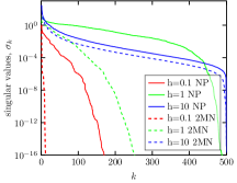
(a) off-diagonal $500\times 500$ block of the kernel matrix

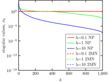
(b) full kernel matrix

Figure 1: GAS1K: singular values with and without two-means (2MN) preprocessing.

h	0.01	0.1	1	10	100
effective rank N/P	1	23	338	129	14
effective rank 2MN	1	1	78	76	12

Table 1: GAS1K: effective rank = number of singular values of the off-diagonal $500\times 500$ $K(1,2)$ block that are $>0.01$, with and without 2MN clustering. Effective rank gets small when $h\to 0$ or $h\to\infty$.

1.1 Main Contributions

We propose to use hierarchical matrix approximations for the kernel. We use both Hierarchically Semi-Separable (HSS) as well as $\mathcal{H}$ matrices. The HSS algorithms are implemented as part of the STRUMPACK library. STRUMPACK — STRUctured Matrix PACKage — is a fast linear solver and preconditioner for sparse and dense systems. One salient feature of STRUMPACK is that the HSS construction uses adaptive randomized sampling for numerical rank detection, which requires a black-box matrix times vector multiplication routine as well as access to selected elements from the kernel matrix (1.1). There is no need to explicitly store the whole matrix $K$; we call this the partially matrix-free interface. This feature is particularly attractive for kernel methods, because forming the complete $K$ may consume too much memory.

Although STRUMPACK works algebraically with any input matrix, different row and column orderings affect the numerical ranks of the off-diagonal blocks, and hence the performance. Intuitively, for an off-diagonal block $K(I,J)$ to have a small rank, the data points in the clusters $I$ and $J$ need to have as little interaction as possible. This suggests a preprocessing step using clustering algorithms, namely, (a) find groups of points with large inter-group distances and small intra-group distances, and (b) permute the rows and columns of the matrix $K$ such that the points of each group have consecutive indices.

Another performance-critical aspect is how the random sampling is performed. If we use traditional matrix-matrix multiplication to perform the sampling $KR$, where $R$ consists of a number of random vectors, the entire solution time will be dominated by this operation. Here, we can exploit the special structure of matrix $K$ and use a faster structured sampling method with an $\mathcal{H}$ matrix.

To summarize, the main contributions of this work are:

• We present an algorithm allowing fast approximate kernel matrix computations with linear scalability of the factorization and solution phases.

• For the preprocessing step, we explore various row and column orderings to improve the efficiency of HSS approximations in kernel methods.

• We use a fast sampling method based on the $\mathcal{H}$ matrix approximation of $K$, removing the bottleneck of the sampling phase for the HSS construction.

• We use the auto-tuning framework OpenTuner for the tuning of the hyperparameters in classification using kernel ridge regression.

• We report scalability experiments up to 1,024 cores, with real-world datasets from the UCI [9] up to $N$=4.5M data points for training, and dimension 784.

We experimented with a number of clustering techniques (including versions of agglomerative and hierarchical clusterings, as well as divisive 2-means, kd-tree and PCA-tree clusterings) and achieved improvements up to $10\times$ in terms of memory usage, with much lower ranks, of the compressed matrix compared to the naive application of STRUMPACK (without clustering) and up to $4\times$ compared to k-d tree based reordering. We believe that the clustering techniques might be useful for more general classes of data related matrices, in order to reveal the implicit hierarchical off-diagonal low-rank structure, and will make them amenable to fast and scalable algorithms. Asymptotically quasi-optimal memory consumption is key for the kernel ridge regression to be able to process large datasets.

1.2 Previous Work

A number of methods have been developed in the intersection of scientific computing and machine learning, with the goal to accelerate kernel methods. Here we give some highlights of the important methods, although we do not have an exhaustive list covering the entire field.

The best rank $r$ approximation of a matrix would be given by direct low-rank matrix factorization methods, based on singular value decomposition. However, even with multiple improvements (in particular, due to the use of randomization [15], see also a survey [20]), the total complexity of such methods stays quadratic in the number of samples $\mathcal{O}(n^{2}\log r)$. They also require creating and storing the entire kernel matrix $K$.

When the kernel matrix exhibits globally low rank, Nyström methods are shown to be among the best methods (see, for example, [6, 22]). Unfortunately, not all kernel matrices can be well approximated by low-rank matrices in a global sense.

Other approximation approaches include fast multipole method (FMM) partitions that try to split the data points into different boxes and quantify interactions between the points that are far apart (such as [24]) – however, it seems that these methods work well only for low dimensional data.

The next idea, also crucial for our work, is to combine the low rank approximation with a clustering of the data points. Some of the previous algorithms using this idea are the following. Clustered Low-Rank Approximation (CLRA, [16] and its parallel version [21]) was created to process large graphs. It starts with the clustering of the adjacency matrix, and then computes a low-rank approximation of each cluster (i.e., diagonal block), e.g. using singular value decomposition. Memory Efficient Kernel Representation (MEKA, [17]) also performs clustering, and then applies Nyström approximation to within-cluster blocks (to avoid computing all within block entries), and introduces a sampling approach to capture between-block information. Block Basis Factorization (BFF, [19]) improves upon MEKA in several ways, including computation of the low-rank basis vectors from a larger space, introducing a more sophisticated sampling procedure, and estimating near-optimal $k$, the number of clusters for the initial data splitting.

Our approach exploits both clustering and low rank property, but in a different way. Instead of initial splitting of data into $k$ clusters, we construct a binary tree of embedded clusters. Then we use low rank property of the off-diagonal sub-blocks of the kernel matrix, corresponding to the inter-cluster links, as well as the hierarchical connection between the clusters (and, respectively, sub-blocks) for efficient approximation of the low rank bases.

The line of work that is closest to ours and also based on off-diagonal low rank is presented in a series of papers [23, 11, 4, 10, 5], where the block-diagonal-plus-low-rank hierarchical matrix format is used to approximate the kernel matrix. The authors first developed an $\mathcal{O}(dN\log N)$ algorithm ASKIT to construct the approximate representation for the kernel matrix [11], and later an $\mathcal{O}(N\log N)$ algorithm INV-ASKIT to perform a factorization of the approximate matrix [4, 5], which can be used as a direct linear solver.

Our current work differs from the INV-ASKIT approach in several ways:

1) we use the $\mathcal{H}$ and HSS matrix formats in the approximation, 2) we use ULV factorization, rather than the Sherman-Morrison-Woodbury formula used in INV-ASKIT, and 3) we compare a number of clustering methods to help reduce the off-diagonal rank, while INV-ASKIT only used the k-d tree ordering.

2 Kernel Ridge Regression for Classification

Ridge regression is probably the most elementary algorithm that can be kernelized. Classical ridge regression is designed to find the linear hyperplane that approximates the data labels well, and at the same time does not have too large coefficients, namely

$$\operatorname{argmin}_{w}\sum_{i=1}^{n}(y_{i}-w\cdot x_{i})^{2}+\lambda\|w\|_{2}^{2},$$

where $x_{i}$ are data points (rows of the data matrix $X$), $y_{i}$’s are their labels, $y=(y_{1},\ldots,y_{n})$ and $w$ is the normal vector to the target hyperplane. It can be proved (see, for example, [7]) that the optimal $w$ is given by

$$\hat{w}:=X^{T}(XX^{T}+\lambda I)^{-1}y.$$

The kernel trick introduces a way to replace the matrix $XX^{T}$ by a certain kernel matrix $K$, effectively substituting the scalar products $x_{i}\cdot x_{j}=X_{ij}$ by the elements $K(x_{i},x_{j})=K_{ij}$, that represent the scalar product in some higher dimensional space.

Specifically, our experimental results for the two-class classification using ridge regression with the Gaussian kernel (1.1) are obtained by the following Algorithm 1:

Input: $X$ – $n\times d$ train data matrix;

      $X^{\prime}$ – $m\times d$ test data matrix;

      $y\in\{\pm 1\}^{n}$ – train labels

Output: $y^{\prime}\in\{\pm 1\}^{m}$ – predicted test labels

Parameters: $h$ – Gaussian width;

      $\lambda$ – regularization parameter

0. Preprocessing step: reorder data points $x_{i}$’s so that $dist(x_{i},x_{j})$ is small if and only if $|i-j|$ is small (see Section 4 for the details).

1. Compute kernel matrix on the train data.

$\quad K_{ij}:=K(x_{i},x_{j})=\exp(-\|x_{i}-x_{j}\|^{2}/(2h^{2}))$

 where data points $x_{i}$ are the rows of $X$, $i=1,\ldots,n$.

2. Compute weight vector $w$ by solving the linear system

$\quad w:=(K+\lambda I)^{-1}y$

3. For each test data sample $x^{\prime}_{i}\in X^{\prime}$, $i=1,\ldots,m$,

compute kernel vector w.r.t. the train data

$\quad K^{\prime}(i)_{j}:=\exp(-\|x_{j}-x^{\prime}_{i}\|^{2}/(2h^{2})),\quad j=1,\ldots n,$

$\quad K^{\prime}(i):=(K^{\prime}(i)_{1},\ldots,K^{\prime}(i)_{n})^{T}$

4. For each $x^{\prime}_{i}\in X^{\prime}$, predict its class label as

$\quad y^{\prime}_{i}:=\operatorname{sign}(w^{T}\cdot K^{\prime}(i))$

Algorithm 1 Gaussian kernel ridge regression

The choice of parameters ($h$, $\lambda$) is based on a particular dataset and usually made by a cross-validation. The prediction accuracy is computed as the fraction of correctly predicted test labels:

$$Acc=\frac{|\{y^{\prime}\equiv\bar{y}^{\prime}\}|}{m},$$ (2.1)

where $\bar{y}^{\prime}\in\{\pm 1\}^{m}$ are the true test labels (and $y^{\prime}\in\{\pm 1\}^{m}$ are predicted test labels).

In Algorithm 1, the most time-consuming computation is solving the linear system during the training stage (Step 2). One key observation is that the final prediction accuracy does not require many digits of the solution weight vector $w$, since it contributes only to the sign calculation in Step 4. Therefore, we can use an inexact but faster linear solver, such as STRUMPACK, to alleviate the performance bottleneck at Step 2. The goal of preprocessing Step 0 is to have matrix $K$ (constructed on Step 1) in an HSS format, at minimum rank.

Other algorithms are also suggested for the kernel matrix compression (see [6, 7]). In [6] the authors show the results of the binary classification by the kernel ridge regression. There does not seem to be one best solution suggested so far.

A possible future work is to fully compare the classification accuracy and the speed with STRUMPACK to that obtained from the method described in [4].

Finally, although Algorithm 1 is defined for two classes, it is easy to adapt it for the multi-class classification. The simplest way to do it is to make one-vs-all predictions. To distinguish between $c>2$ classes, we would need to construct $c$ binary classifiers, that differ from the Algorithm 1 only in Step 4. Namely,

$$y^{\prime}(c)_{i}:=|w^{T}(c)\cdot K^{\prime}(i)|,$$

which interprets now as the level of confidence that $i$-th test point belongs to the class $c$. Then the class of $x^{\prime}_{i}$ is defined as

$$c(i):=\operatorname{argmax}_{c}y^{\prime}(c)_{i}.$$

3 Data Sparse Formats

In this section, we briefly describe two hierarchical matrix formats used in this work, the hierarchically semi-separable (HSS) representation, in Section 3.1, and the hierarchical $\mathcal{H}$ matrix format, in Section 3.2. These matrix representations use a hierarchical partitioning of the matrix into smaller blocks, some of which can be compressed using low-rank approximations.

The two hierarchical matrix formats play different roles in this work. The HSS matrix has higher construction cost (if we use traditional dense matrix multiplication in the sampling stage) but very low factorization and solve cost, whereas the $\mathcal{H}$ matrix has lower construction and matrix-vector multiplication cost but higher factorization cost. Our approach is to use the fast matrix-vector multiplication capability of the $\mathcal{H}$ matrix to speed up the HSS matrix construction.

3.1 Hierarchically Semi-Separable Matrix Representation

Figure 2: Illustration of an HSS matrix using $4$ levels. Diagonal blocks are partitioned recursively. Gray blocks denote the basis matrices.

Figure 3: Tree for Figure 3, using postordering. All nodes except the root store $U_{i}$ and $V_{i}$. Leaves store $D_{i}$, non-leaves $B_{ij}$, $B_{ji}$

The HSS representation, as illustrated in Figure 3, uses a block $2\times 2$ partitioning of a matrix $A\in\mathbb{R}^{n\times n}$, with a similar partitioning applied recursively to the diagonal blocks. This recursive partitioning defines a tree, as illustrated in Figure 3. With a node $i$ in the tree, an index set $I_{i}\subset\left\{1,\dots,n\right\}$ is associated. At the last level of the recursion, the diagonal blocks, i.e., $A(I_{i},I_{i})$ are stored as (small) dense matrices. All off-diagonal blocks $A_{ij}$ are compressed using a low-rank factorization $U_{i}B_{ij}V_{j}^{T}$. Moreover, the column basis matrix $U_{i}$, for a node $i$ with children $c_{1}$ and $c_{2}$ in the hierarchy is defined as $U_{i}=\begin{bmatrix}U_{c_{1}}&0\\ 0&U_{c_{2}}\end{bmatrix}\tilde{U}_{i}$, and hence only the smaller matrix $\tilde{U}_{i}$ is stored at node $i$. Only at the leaf nodes, where $U_{i}\equiv\tilde{U}_{i}$, are the $U_{i}$ stored explicitly. A similar relation holds for the $V_{i}$ basis matrices, and is referred to as the nested basis property. The HSS data structure is implemented in the STRUMPACK (STRUctured Matrix PACKage) library [32, 14, 18]. STRUMPACK is a sparse direct solver and preconditioner. It uses HSS compression for the sparse triangular factors. However, the HSS kernels implemented in STRUMPACK can also be used directly on dense matrices, for instance coming from integral equations, the boundary element method, electromagnetic scattering etc. For the construction of HSS matrices, STRUMPACK implements a randomized algorithm from [12]. This algorithm requires a matrix times (multiple) vector product for the random sampling phase. A fast multiplication routine is crucial to get good performance. STRUMPACK also implements a ULV factorization [33] algorithm, and a corresponding routine to solve a linear system with the factored HSS matrix. If a fast sampling routine is available, both HSS compression and factorization have $\mathcal{O}(rn)$ complexity, with $r$ the maximum HSS rank.

3.2 $\mathcal{H}$ Matrix Representation

Figure 4: Example of a symmetric $\mathcal{H}$ matrix using $4$ levels. Off-diagonal gray blocks denote low-rank factorizations.

$\mathcal{H}$ (and $\mathcal{H}^{2}$) matrices are yet another group of hierarchical matrix formats for building fast linear solvers. Contrary to HSS, where all off-diagonal blocks are low-rank compressed (weak admissibility), $\mathcal{H}$ formats only compress the well-separated sub-blocks (strong admissibility). For example, the off-diagonal blocks in Figure 4 are recursively partitioned into smaller ones and low-rank compressed if they are well-separated (i.e., admissible). Strong admissibility leads to well-bounded numerical ranks for admissible blocks in linear systems arising from high-dimensional applications (e.g., 3D acoustic and electromagnetic scattering problems and high-dimensional kernel matrices). Therefore, the construction of an $\mathcal{H}$ matrix for the kernel matrix can be performed in quasi-linear time and memory. However, it is well-known that the inversion of $\mathcal{H}$ matrices requires significantly higher computation overhead when compared to weak-admissibility solvers, such as those based on HSS. Experiments showed that using an $\mathcal{H}$ solver to solve the linear system in Step 2 of Algorithm 1 is much slower than HSS due to the inversion bottleneck. Therefore, instead of using the $\mathcal{H}$ solver to solve the system directly, we use it only to compress the kernel matrix and then to accelerate the HSS construction as described below.

Recall that during the HSS construction, STRUMPACK requires rapid multiplication of the kernel matrix and its transpose to random vectors in the sampling stage. Instead of direct application of the matrices to vectors, one can leverage Fast Gauss Transform [24], analytical/algebraic fast multipole methods to accelerate the construction. To this end, we tailored and adapted an $\mathcal{H}$ solver [25] to kernel matrices. The low-rank representation of an admissible block is computed via a hybrid-ACA scheme that constructs a low-rank factorization of its submatrix that represents interactions between closely located points. The selection of the submatrix, however, is based on a trade-off between efficiency and accuracy of the factorization.

4 Dataset Clustering

This section discusses how appropriate preprocessing of the input data can drastically improve the effectiveness of HSS approximation. Section 4.3 describes a number of clustering algorithms to reduce the ranks of the HSS off-diagonal blocks.

4.1 Kernel Matrices and HSS Structure

Intuitively, a kernel matrix can be viewed as a similarity matrix $K=(K_{ij})_{i,j=1,\ldots,n}$, where

$$K_{ij}=\text{ similarity score between }x_{i}\text{ and }x_{j}.$$ (4.1)

Such a matrix $K$, defined by a set of objects $x_{1},\ldots,x_{n}$ is always square and symmetric. These objects can be anything from two integers, two real valued vectors, to particles, words etc., provided that we know how to compare them. Kernel matrices are used to improve algorithms to classify these objects, e.g. allowing more sophisticated boundaries between classes. The Gaussian kernel (1.1), studied throughout this paper, is but one example kernel matrix; though probably the most widely used one. Let $x_{1},\ldots,x_{n}$ be data points in $d$ dimensional space $\mathbb{R}^{d}$, which are said to be “similar” if they are close to each other in Euclidean distance.

Broadly speaking, the preprocessing takes advantage of the fact that the interaction between two well separated clusters of data points can be approximated accurately when expressed in terms of the interaction between a smaller number of representative points from each cluster. This same idea is used very successfully in tree-codes [26], the fast multipole method (FMM) [27], matrix skeletonization [29] and interpolative decomposition [28]. Hence, splitting the input data in clusters with large inter cluster distances leads to lower ranks for the off-diagonal blocks of $K$, and hence less memory usage and faster algorithms. This low rank property is illustrated in Figure 1(a) with and without preprocessing, and it motivates the idea of using an HSS solver like STRUMPACK to speed up kernel matrix computations. Due to the exponential decay of the Gaussian kernel, many elements in the kernel matrix, away from the diagonal, are actually negligibly small. Furthermore, the low rank pattern is proven in [30].

4.2 Preprocessing by Data Clustering

Reordering the input data $x_{1},\ldots,x_{n}$ corresponds to applying a permutation symmetrically to the rows and columns of the kernel matrix. Preprocessing is applied in the following steps:

1. Partition the data points in two clusters with large inter-group distance and small intra-group distance.

2. Reorder the input data such that points in the same group occupy consecutive indices, increasing the data-sparsity of the off-diagonal blocks in the corresponding kernel matrix.

3. Use these two index ranges to partition the corresponding node in the HSS tree, as illustrated in Figure 3. Repeat Steps 1 and 2 recursively for both partitions computed in Step 1.

Step 1 suggests that this preprocessing is a clustering problem. The task of finding clusters of points is widely studied, with numerous clustering algorithms described in the literature, without there being one absolute best solution. Different algorithms perform better for different applications and clustering quality can often be traded for execution time or memory usage (see, for example, [7]).

Our specific requirements for an optimal clustering come from (a) the properties of the HSS data structure and (b) the general goal to minimize memory usage of the hierarchical matrix data structures. The latter requires a clustering algorithm that does not construct the kernel matrix $K$, or an equivalent $n\times n$ distance matrix, explicitly. It should also be fast, preferably $\mathcal{O}(n)$ or $\mathcal{O}(n\log n)$. The HSS partitioning is defined by a hierarchical structure; a possibly unbalanced and incomplete tree. However, in order to be able to exploit enough parallelism and to reduce memory usage, the tree should be deep enough, i.e., have a small enough maximum leaf size.

Rather than the standard dissimilarity metrics measuring clustering quality, the following performance metrics are used in this work:

• Memory (MB): the sum of the memory used by all the individual smaller matrices in the HSS structure: $D_{i}$, $U_{i}$, $V_{i}$, $B_{ij}$, $B_{ji}$ (see Section 3.1).

• Accuracy of classification (%): the percentage of correctly predicted labels in the test set (with the parameters $h$ and $\lambda$ chosen based on the validation set).

• Time (s): the time required for compression into HSS form, for factorization of the HSS matrix, and for solution of the linear system.

• Maximum rank: the largest rank encountered in any of the off-diagonal blocks of the HSS structure.

4.3 Selected Preprocessing Methods

Previous work on approximation of kernel matrices used reorderings based on ball tree clustering, see for instance [23, 19], or based on k-d tree clustering, see [13].

We have compared a variety of different clustering techniques and their variations, both divisive and agglomerative, on several real world datasets. Each of the clustering algorithms used in the numerical results section are divisive, i.e., they use a top-down, recursive split of the input points into two separated clusters. The recursive splitting continues while clusters are bigger than a certain leaf size, chosen to be $16$ for HSS. This leaf size is the size of the diagonal blocks in the HSS structure. The leaf size should not affect the accuracy of the hierarchical matrix representation, but it affects the memory usage.

Agglomerative methods, in contrast to the divisive strategy, although very good at reducing memory and ranks of the HSS structure, did not show competitive performance. We experimented with a variety of hierarchical clustering methods, and typical disadvantages arising were either very unbalanced class sizes, or lack of parallelism ($\mathcal{O}(n^{2})$ scaling, requiring to construct and store the complete distance matrix).

For the experiments we consider four orderings:

No preprocessing (NP): This is the baseline to compare with: the input is not reordered, no information about mutual distances is used to permute the matrix. The HSS tree is a complete binary tree, constructed by recursively splitting index sets in two equal ($\pm 1$) parts.

Recursive two-means (2MN) This special case of the well-known $k$-means clustering algorithm is applied recursively to define the HSS tree. $K$-means is an iterative algorithm which works as follows. Pick two points (at random) to represent two clusters; for each point in the data set, compute the distance to those two points and find which one is closer, assign points to the closest cluster; compute the center off each cluster and take that as the new representative point of the cluster; repeat until no points change cluster. Typically only a few iterations are required. However, the procedure is relatively sensitive to the choice of initial cluster representatives. Initially, we pick one point randomly and select the second one with a probability proportional to the distance from the first one.

K-d tree (KD) The data is split along the coordinate dimension of maximum spread, at the mean value for that coordinate. Splitting at the mean is sensitive to outliers, and can lead to very unbalanced trees. Alternatively, splitting at the median value always results in a well balanced tree. However, using the mean leads to lower memory usage and when the input data is normalized, the sensitivity with respect to outliers is less pronounced. If the resulting clusters are still too unbalanced, i.e., when ($100\cdot\text{size(cluster1)}<\text{size(cluster2)}$), we fall back to splitting at the median. This clustering is applied recursively, where at each step of the recursion, a new direction of maximum spread is determined.

Principal component analysis (PCA) At each step of the recursive clustering, the data is split according to the mean value in the projection onto the first principal component (i.e. direction of the maximum spread). We expect this to be a better clustering than the simpler k-d tree method, at a somewhat higher cost.

5 Numerical Results

Experiments were performed at NERSC’s Cori supercomputer. Each Cori node has two sockets, each socket is a 16-core Intel Xeon Processor E5-2698 v3 (“Haswell”) processor at 2.3 GHz and 128 GB DDR4 memory.

5.1 Datasets Description

We use real-world datasets coming from life sciences, physical sciences and artificial intelligence. The reported datasets are: SUSY, HEPMASS (high-energy physics, Monte Carlo simulated kinematic properties of the particles in the accelerator), COVTYPE (predicting forest cover type from cartographic variables), GAS (measurements from chemical sensors to distinguish between gases with different concentration levels), PEN and LETTER (handwritten digits and letters recognition). All mentioned datasets are taken from the UCI repository [9]. Finally, to illustrate the performance on a dataset with large dimension, we used the MNIST dataset of handwritten digits (extended 8M dataset, including shifts and rotations of the classical MNIST digits dataset) [3].

For the datasets having multiple classes we perform one-vs-all prediction. In particular, in MNIST and PEN we predict digit 5, in LETTER we predict letter A, in COVTYPE – type 3 (Ponderosa Pine), in GAS – gas number 5. Prediction accuracy might differ significantly if one would predict some other class.

5.2 Preprocessing Comparison

Dataset (dim)	Memory (MB)				Acc
	N/P	KD	PCA	2MN
SUSY (8)	499	344	242	190	80.1%
h = 1, $\lambda$ = 4
LETTER (16)	315	237	91	51	100%
h = .5, $\lambda$ = 1
PEN (16)	445	227	133	58	99.8%
h = 1, $\lambda$ = 1
HEPMASS (27)	577	505	542	435	91.1%
h = 1.5, $\lambda$ = 2
COVTYPE (54)	655	344	120	45	97.1%
h = 1, $\lambda$ = 1
GAS (128)	264	65	29	25	99.5%
h = 1.5, $\lambda$ = 4
MNIST (784)	40	164	43	36	97.2%
h = 4, $\lambda$ = 3

Table 2: Memory usage is in MB, accuracy is in % of the test size (1K for all datasets). All train sets have 10K samples, normalized to zero mean and standard deviation one.

We report in Table 2 our main performance metrics – memory and accuracy. The table compares different preprocessing methods with seven datasets. Memory usage heavily depends on parameter $h$, which is illustrated on the GAS10K dataset in Fig. 5. Furthermore, in the context of hierarchical low-rank approximations, memory is proportional to performance, since the number of flops is proportional to the numerical ranks of the approximation.

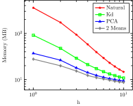
Figure 5: GAS10K dataset, 1K test, $\lambda=4$. Memory usage for various $h$ and clustering methods.

Recursive two means (2MN) preprocessing shows best memory performance for all the $h$ values. With STRUMPACK tolerance set to be at most 0.1, the prediction accuracy does not seem to depend on the preprocessing methods, see Table 2. Moreover, for the 10K datasets reported in Table 2 this accuracy matches the accuracy we get using the full non-compressed kernel matrix in Algorithm 1. The main disadvantage of 2MN is higher variance of the resulting rank, and, to lower extent, memory. The numbers reported for 2MN are average over three runs of the algorithm. The instability can be avoided by choosing non-random start points at every step of two means clustering. All datasets were normalized to have zero mean and unit standard deviation columns. The experiments with non-normalized datasets, and with datasets normalized to have maximum absolute value one have shown significantly lower accuracy (e.g. for MNIST2M dataset).

5.3 Hyperparameter Tuning

The algorithm parameters $h$ and $\lambda$ are key to determine the predictive capabilities of the matrix approximation. Consider the HSS approximation of matrix $K+\lambda I$ used in this work. When the parameter $\lambda$ changes, we only need to update the diagonal entries of the HSS matrix, and there is no need to perform HSS construction again.

However, a change to $h$ requires to perform HSS reconstruction from scratch, which is costly. There are theoretical estimates that limit the search space for $h$ [34], but it is problem dependent. A fine grid search is too costly, see Figure 6(a). In contrast, the black-box optimization techniques in the OpenTuner package [31] in Figure 6(b) required only 100 runs and converged to a tuning parameter with better prediction accuracies than grid search. This technique drastically reduced the computational requirements to select $h$ and $\lambda$.

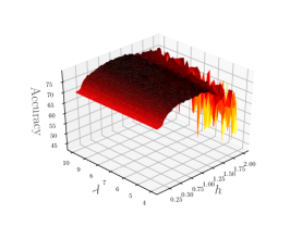
(a) Grid search

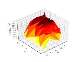
(b) OpenTuner

Figure 6: Left: grid search of $128^{2}$ runs for the SUSY dataset. Right: black-box optimization with 100 runs.

5.4 Large-Scale Prediction

The appeal of using optimal algorithms is the ability to process large amount of data. Table 3 shows the predictive capabilities of this method by using datasets that allow the training step to use data points in the order of millions of entries, at different dimensions. The reported prediction accuracy is tested against a test subset of the complete dataset, that is, labeled data that were not considered during training or hyperparameter tuning.

Dataset	$N$	$d$	$h$	$\lambda$	Acc
SUSY	4.5M	8	0.08	10	73%
MNIST	1.6M	784	1.1	10	99%
COVTYPE	0.5M	54	0.07	0.3	99%
HEPMASS	1.0M	27	0.7	0.5	90%

Table 3: Large-scale prediction on test data.

5.5 Asymptotic Complexity

When hierarchical matrix approximations have constant ranks, such as in a broad class of elliptic partial differential equations, the HSS memory consumption are number of operations are strict $\mathcal{O}(N)$; however, recent theoretical results show that the numerical rank of kernel matrices in high dimension depends on the dimension of the dataset [30]. We experimentally confirm this rank growth in the additional memory requirements (Figure 7(a)) and time for factorization (Figure 7(b)).

The major benefit of the near-linear complexity in factorization and memory is that this method enables the use of kernel matrices for the large datasets. As an example, storing a 1M dense matrix requires 8,000GB, whereas the HSS construction used in this work just required 1.3 GB. A similar argument can be made for the factorization of such a matrix, with which a traditional Cholesky factorization of $\mathcal{O}(n^{3})$ is intractable at this scale.

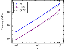
(a) Memory consumption of the compressed matrices.

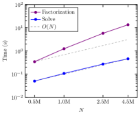
(b) Time of the factorization and solve stages with HSS.

Figure 7: Asymptotic complexity of memory and time using the SUSY $N$=4.5M dataset.

5.6 Performance Details

Table 4 shows the performance of the main algorithmic steps of our method. The first step is the $\mathcal{H}$ construction to accelerate the otherwise $\mathcal{O}(n^{2})$ HSS sampling. For instance, with naïve HSS sampling, the construction process of a kernel matrix required more than 2 hours for $n$=0.5M, now with the $\mathcal{H}$ matrix sampling we can construct an HSS matrix for $n$=4.5M in about 10 minutes.

Currently, our $\mathcal{H}$ matrix implementation is only a prototype code and is not optimized at all. Although it enabled us to experiment with datasets as large as reported in the literature, it is only capable of effectively using a subset of the processes that the HSS code can use (factorization and solve). Nonetheless, the successful synergy between the $\mathcal{H}$ and HSS matrix formats motivates our future work to develop a robust and more scalable distributed memory $\mathcal{H}$ matrix code. With that, we expect to achieve much faster $\mathcal{H}$ construction time and sampling time.

	SUSY		COVTYPE
Cores	32	512	32	512
$\mathcal{H}$ construction	173.7	18.3	36.5	32.2
HSS construction	3344.4	726.7	432.3	239.7
$\longrightarrow$ Sampling	2993.5	662.1	305.2	178.4
$\longrightarrow$ Other	350.9	64.6	127.1	61.3
Factorization	14.2	3.3	26.5	4.6
Solve	0.5	0.3	0.5	0.4

Table 4: Timing details in seconds for the SUSY and COVTYPE datasets.

Figure 8 shows a strong scaling experiment up to 1,024 cores of the factorization phase of the kernel computation for the datasets used in Table 4. As mentioned in the previous section, a scalable and fast factorization for large datasets is critical for kernel matrix computations. We refer the reader to [14] for the distributed memory parallelization aspects of the ULV factorization used in this work. At large core count, the number of degrees of freedom per core decreases dramatically, while communication time starts to dominates, hence runtime starts to depart from the linear scaling line. The wall-clock time, however, is in the order of a handful of seconds even for the largest dataset considered in this work. Note that even though the SUSY dataset is larger than the MNIST dataset the overall factorization time is larger for MNIST, this is due to the fact that the dimension of MNIST is bigger than SUSY, and the dimension of the dataset has a direct effect on the necessary ranks of the approximation, and therefore in the required number of operations.

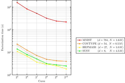
Figure 8: Strong scaling of large-scale datasets.

6 Conclusions

We showed that the HSS linear solvers, such as the one as implemented in STRUMPACK, are useful for a completely new area of machine learning applications. We proposed to use several relatively sophisticated ways to preprocess the kernel matrix (i.e. cluster points in the dataset), and showed that the preprocessing can significantly improve the compression rate. In all the literature we have seen the authors used either natural or k-d tree preprocessing and did not perform comparison of the various ordering techniques.

We presented performance data of an HSS-based complexity solver for kernel matrices scaling up to 1,024 cores of the NERSC Cori supercomputer. The construction of the HSS matrices used different preprocessing methods to minimize memory consumption for the solution of the classification task on high dimensional datasets at high prediction accuracy.

Preliminary results show that an incomplete factorization as described in this work might be an effective preconditioner for the iterative solution of kernel matrices. We will report on the trade-offs and effectiveness of this strategy in future work.

References

- [1] El Alaoui, A. and Mahoney, M.W., 2014. Fast randomized kernel methods with statistical guarantees. stat, 1050, p.2.
- [2] Bach, F., 2013, June. Sharp analysis of low-rank kernel matrix approximations. In Conference on Learning Theory (pp. 185-209).
- [3] Chang, C.C. and Lin, C.J., 2011. LIBSVM: a library for support vector machines. ACM transactions on intelligent systems and technology (TIST), 2(3), p.27.
- [4] Yu, Chenhan D., March, W.B., Xiao, B. and Biros, G., 2016, May. INV-ASKIT: a parallel fast direct solver for kernel matrices. In Parallel and Distributed Processing Symposium, 2016 IEEE International (pp. 161-171). IEEE.
- [5] Yu, Chenhan D., March, W.B., Xiao, B. and Biros, G., 2017, May. An parallel fast direct solver for kernel matrices. In Parallel and Distributed Processing Symposium, 2017 IEEE International.
- [6] Gittens, A. and Mahoney, M.W., 2016. Revisiting the Nyström method for improved large-scale machine learning. The Journal of Machine Learning Research, 17(1), pp.3977-4041.
- [7] Hastie, T., Tibshirani, R. and Friedman, J., 2009. Unsupervised learning. In The elements of statistical learning (pp. 485-585). Springer, New York, NY.
- [8] Hofmann, T., Schölkopf, B. and Smola, A.J., 2008. Kernel methods in machine learning. The annals of statistics, pp.1171–1220.
- [9] Lichman, M. 2013. UCI Machine Learning Repository http://archive.ics.uci.edu/ml. Irvine, CA: University of California, School of Information and Computer Science.
- [10] March, W.B., Xiao, B., Tharakan, S., Chenhan, D.Y. and Biros, G., 2015, November. A kernel-independent FMM in general dimensions. In High Performance Computing, Networking, Storage and Analysis, 2015 SC-International Conference for (pp. 1-12). IEEE.
- [11] March, W.B., Xiao, B. and Biros, G., 2015. ASKIT: Approximate skeletonization kernel-independent treecode in high dimensions. SIAM Journal on Scientific Computing, 37(2), pp.A1089-A1110.
- [12] Martinsson, P.G., 2011. A fast randomized algorithm for computing a hierarchically semiseparable representation of a matrix. SIAM Journal on Matrix Analysis and Applications, 32(4), pp.1251–1274.
- [13] Omohundro, S.M., 1989. Five balltree construction algorithms (pp. 1-22). Berkeley: International Computer Science Institute.
- [14] Rouet, F.H., Li, X.S., Ghysels, P. and Napov, A., 2016. A distributed-memory package for dense hierarchically semi-separable matrix computations using randomization. ACM Transactions on Mathematical Software (TOMS), 42(4), p.27.
- [15] Sarlos, T., 2006, October. Improved approximation algorithms for large matrices via random projections. In Foundations of Computer Science, 2006. FOCS’06. 47th Annual IEEE Symposium on (pp. 143-152). IEEE.
- [16] Savas, B. and Dhillon, I.S., 2011, April. Clustered low rank approximation of graphs in information science applications. In Proceedings of the 2011 SIAM International Conference on Data Mining (pp. 164-175). Society for Industrial and Applied Mathematics.
- [17] Si, S., Hsieh, C.J. and Dhillon, I., 2014, January. Memory efficient kernel approximation. In International Conference on Machine Learning (pp. 701–709).
- [18] STRUMPACK website http://portal.nersc.gov/project/sparse/strumpack/
- [19] Wang, R., Li, Y., Mahoney, M.W. and Darve, E., 2015. Structured block basis factorization for scalable kernel matrix evaluation. preprint arXiv:1505.00398.
- [20] Mahoney, M.W., 2011. Randomized algorithms for matrices and data. Foundations and Trends® in Machine Learning, 3(2), pp.123-224.
- [21] Sui, X., Lee, T.H., Whang, J.J., Savas, B., Jain, S., Pingali, K. and Dhillon, I., 2012, September. Parallel clustered low-rank approximation of graphs and its application to link prediction. In International Workshop on Languages and Compilers for Parallel Computing (pp. 76-95). Springer, Berlin, Heidelberg.
- [22] Williams, C.K. and Seeger, M., 2001. Using the Nyström method to speed up kernel machines. In Advances in neural information processing systems (pp. 682-688).
- [23] Yu, C.D., Huang, J., Austin, W., Xiao, B. and Biros, G., 2015, November. Performance optimization for the k-nearest neighbors kernel on x86 architectures. In Proceedings of the International Conference for High Performance Computing, Networking, Storage and Analysis (p. 7). ACM. Vancouver
- [24] Yang, C., Duraiswami, R., Gumerov, N.A. and Davis, L., 2003, October. Improved fast Gauss transform and efficient kernel density estimation. In Ninth International Conference on Computer Vision (p. 664). IEEE.
- [25] H. Guo and Y. Liu and J. Hu and E. Michielssen, 2017. A butterfly-based direct integral-equation solver using hierarchical LU factorization for analyzing scattering from electrically large conducting objects. IEEE Transactions on Antennas and Propagation, 65(9), p.4742.
- [26] J. Barnes and P. Hut, 1986. A hierarchical force-calculation algorithm A fast algorithm for particle simulations. Nature, 324, p.446.
- [27] L. Greegard and V. Rokhlin, 1987. A fast algorithm for particle simulations. Journal of Computational Physics, 73, p.325.
- [28] Cheng, Hongwei, Zydrunas Gimbutas, Per-Gunnar Martinsson, and Vladimir Rokhlin, 2005. On the compression of low rank matrices. SIAM Journal on Scientific Computing, 26(4), p.1389.
- [29] S.A.Goreinov, E.E.Tyrtyshnikov and N.L.Zamarashkin, 1997. A theory of pseudoskeleton approximations. Linear Algebra and its Applications, 261(1), p.1.
- [30] Wang, R., Li, Y., and Darve, E., 2017. On the numerical rank of radial basis function kernel matrices in high dimension. arXiv:1706.07883.
- [31] J. Ansel and S. Kamil and K. Veeramachaneni and J. Ragan-Kelley and J. Bosboom and U. M. O’Reilly and S. Amarasinghe, 2014. OpenTuner: An extensible framework for program autotuning. In 23rd International Conference on Parallel Architecture and Compilation Techniques (PACT) (p. 303-315). IEEE.
- [32] Ghysels, P., Li, X. S., Gorman, C. and Rouet, F. H., 2017. A robust parallel preconditioner for indefinite systems using hierarchical matrices and randomized sampling, IPDPS 2017, pp.897–906. IEEE
- [33] Chandrasekaran, S., Gu, M. and Pals, T, 2006. A fast ULV decomposition solver for Hierarchically Semiseparable representations, SIAM SIMAX, 28(3), pp.603–622.
- [34] W. Silverman, 1986. Density Estimation for Statistics and Data Analysis, Chapman and Hall.
- [35] William B. March, George Biros, 2017. Far-field compression for fast kernel summation methods in high dimensions. Applied and Computational Harmonic Analysis. volume 43, issue 1, pages 39-75.