Parallel Numerical Tensor Methods for High-Dimensional PDEs

Abstract

High-dimensional partial-differential equations (PDEs) arise in a number of fields of science and engineering, where they are used to describe the evolution of joint probability functions. Their examples include the Boltzmann and Fokker-Planck equations. We develop new parallel algorithms to solve high-dimensional PDEs. The algorithms are based on canonical and hierarchical numerical tensor methods combined with alternating least squares and hierarchical singular value decomposition. Both implicit and explicit integration schemes are presented and discussed. We demonstrate the accuracy and efficiency of the proposed new algorithms in computing the numerical solution to both an advection equation in six variables plus time and a linearized version of the Boltzmann equation.

1 Introduction

High-dimensional partial-differential equations (PDEs) arise in a number of fields of science and engineering. For example, they play an important role in modeling rarefied gas dynamics [1], stochastic dynamical systems [2, 3, 4], structural dynamics [5, 6], turbulence [7, 8, 9, 10], biological networks [11], and quantum systems [12, 13]. In the context of kinetic theory and stochastic dynamics, high-dimensional PDEs typically describe the evolution of a (joint) probability density function (PDF) of system states, providing macroscopic, continuum descriptions of Langevin-type stochastic systems. Classical examples of such PDEs include the Boltzmann equation [1] and the Fokker-Planck equation [14]. More recently, PDF equations have been used to quantify uncertainty in model predictions [15].

High dimensionality and resulting computational complexity of PDF equations can be mitigated by using particle-based methods [8, 16]. Well known examples are direct simulation Monte-Carlo (DSMC) [17] and the Nambu-Babovsky method [18]. Such methods preserve physical properties of a system and exhibit high computational efficiency (they scale linearly with the number of particles), in particular in simulations far from statistical equilibrium [19, 20]. Moreover, these methods have relatively low memory requirements since the particles tend to concentrate where the distribution function is not small. However, the accuracy of particle methods may be poor and their predictions are subject to significant statistical fluctuations [20, 21, 22]. Such fluctuations need to be post-processed appropriately, for example by using variance reduction techniques. Also, relevance and applicability of these numerical strategies to PDEs other than kinetic equations are not clear. To overcome these difficulties, several general-purpose algorithms have been recently proposed to compute the numerical solution to rather general high-dimensional linear PDEs. The most efficient techniques, however, are problem specific [23, 24, 25, 16]. For example, in the context of kinetic methods, there is an extensive literature concerning the (six-dimensional) Boltzmann equation and its solutions close to statistical equilibrium. Deterministic methods for solving such problems include semi-Lagrangian schemes and discrete velocity models. The former employ a fixed computational grid, account for transport features of the Boltzmann equation in a fully Lagrangian framework, and usually adapt operator splitting. The latter employ a regular grid in velocity and a discrete collision operator on the points of the grid that preserves the main physical properties (see §3 and §4 in Di Marco and Pareschi [16] for an in-depth review of semi-Lagrangian methods and discrete velocity models for kinetic transport equations, respectively).

We develop new parallel algorithms to solve high-dimensional partial differential equations based on numerical tensor methods [26]. The algorithms we propose are based on canonical and hierarchical tensor expansions combined with alternating least squares and hierarchical singular value decomposition. The key element that opens the possibility to solve high-dimensional PDEs numerically with tensor methods is that tensor approximations proved to be capable of representing function-related $N$-dimensional data arrays of size $Q^{N}$ with log-volume complexity $\mathcal{O}(N\log(Q))$. Combined with traditional deterministic numerical schemes (e.g., spectral collocation method [27], these novel representations allow one to compute the solution to high-dimensional PDEs using low-parametric rank-structured tensor formats.

This paper is organized as follows. In Section 2 we discuss tensor representations of $N$-dimensional functions. In particular, we discuss canonical tensor decomposition and hierarchical tensor networks, including hierarchical Tucker and tensor train expansions. We also address the problem of computing tensor expansion via alternating least squares. In Section 3 we develop several algorithms that rely on numerical tensor methods to solve high-dimensional PDEs. Specifically, we discuss schemes based on implicit and explicit time integration, combined with dimensional splitting, alternating least squares and hierarchical singular value decomposition. In Section 4 we demonstrate the effectiveness and computational efficiency of the proposed new algorithms in solving both an advection equation in six variables plus time and a linearized version of the Boltzmann equation.

2 Tensor Decomposition of High-Dimensional Functions

Consider a multivariate scalar field $f(\bm{z}):D\subseteq\mathbb{R}^{N}\rightarrow\mathbb{R}$. In this section we briefly review effective representations of $f$ based on tensor methods. In particular, we discuss the canonical tensor decomposition and hierarchical tensor methods, e.g., tensor train and hierarchical Tucker expansions.

2.1 Canonical Tensor Decomposition

The canonical tensor decomposition of the multivariate function $f(\bm{z}):D\subseteq\mathbb{R}^{N}\rightarrow\mathbb{R}$ is a series expansion of the form

$$f(\bm{z})\simeq\sum_{l=1}^{r}\prod_{k=1}^{N}G^{l}_{j}(z_{j}),$$ (1)

where $G^{l}_{i}(z_{i}):\mathbb{R}\rightarrow\mathbb{R}$ are one-dimensional functions usually represented relative to a known basis $\{\phi_{1},...,\phi_{Q}\}$, i.e.,

$$G^{l}_{i}(z_{i})=\sum_{k=1}^{Q}\beta_{ik}^{l}\phi_{k}(z_{i}).$$ (2)

The quantity $r$ in (1) is called separation rank. Although general/computable theorems relating a prescribed accuracy of the representation of $f(\bm{z})$ to the value of the separation rank $r$ are still lacking, there are cases where the expansion (1) is exponentially more efficient than one would expect a priori [28].

Alternating Least Squares (ALS) Formulation

Development of robust and efficient algorithms to compute (1) to any desired accuracy is still a relatively open question (see [29, 30, 31, 32, 23] for recent progresses). Computing the tensor components $G_{k}^{l}(z_{k})$ usually relies on (greedy) optimization techniques, such as alternating least squares (ALS) [33, 34, 29, 28] or regularized Newton methods [30], which are only locally convergent [35], i.e., the final result may depend on the initial condition of the algorithm.

In the least-squares setting, the tensor components $G^{l}_{j}(z_{j})$ are computed by minimizing a norm of the residual,

$$R(\bm{z})=f(\bm{z})-\sum_{l=1}^{r}\prod_{k=1}^{N}G^{l}_{j}(z_{j}),$$ (3)

with respect to the $rNQ$ degrees of freedom $\beta_{hj}^{n}$ i.e.,

$$\min_{\beta_{hj}^{n}}\left\|R(\bm{z})\right\|.$$ (4)

Assuming $f(\bm{z})$ to be periodic in the hyper-cube $D=[-b,b]^{N}$ ($b>0$), we define the norm $\|\cdot\|$ as a standard $L_{2}$ norm

$$\left\|R(\bm{z})\right\|_{L_{2}}^{2}= \int_{-b}^{b}\cdots\int_{-b}^{b}R(\bm{z})^{2}\text{d}\bm{z},$$

$$= \int_{-b}^{b}\cdots\int_{-b}^{b}\left[f(\bm{z})-\sum_{n=1}^{r}\prod_{k=1}^{N}\left(\sum_{s=1}^{Q}\beta_{ks}^{n}\phi_{s}(z_{k})\right)\right]^{2}\text{d}\bm{z}.$$ (5)

In the alternating least-squares (ALS) paradigm, we compute the minimizer of the residual (3) by splitting the non-convex optimization problem (4) into a sequence of convex low-dimensional convex optimization problems. To illustrate the method, let us define vectors

$$\bm{\beta}_{1}=(\beta^{1}_{11},...,\beta^{1}_{1Q},...,\beta^{r}_{11},...,\beta^{r}_{1Q})^{T},\quad\cdots,\quad\bm{\beta}_{N}=(\beta^{1}_{N1},...,\beta^{1}_{NQ},...,\beta^{r}_{N1},...,\beta^{r}_{NQ})^{T}.$$ (6)

Each $\bm{\beta}_{i}$ collects the degrees of freedom of all functions $\{G^{1}_{i}(z_{i}),...,G^{r}_{i}(z_{i})\}$ depending on $z_{i}$. Next, the optimization problem (4) is split into a sequence of convex optimization problems,

$$\min_{\bm{\beta}_{1}}\left\|R\right\|_{L_{2}}^{2},\quad\cdots,\quad\min_{\bm{\beta}_{N}}\left\|R\right\|_{L_{2}}^{2}.$$ (7)

This sequence is not equivalent to the full problem (4) because, in general, it does not allow one to compute the global minimizer of (4) [35, 36, 37, 38]. The Euler-Lagrange equations associated with (7) are of the form

$$\bm{A}_{j}\bm{\beta}_{j}=\bm{g}_{j}\qquad j=1,\ldots,N,$$ (9)

where

$$\bm{A}_{j}=\left[\begin{array}[]{cccc}A^{11}_{j11}\cdots A^{11}_{j1Q}&A^{12}_{j11}\cdots A^{12}_{j1Q}&\cdots&A^{1r}_{j11}\cdots A^{1r}_{j1Q}\\ \vdots&\vdots&\vdots&\vdots\\ A^{11}_{jQ1}\cdots A^{11}_{jQQ}&A^{12}_{jQ1}\cdots A^{12}_{jQQ}&\cdots&A^{1r}_{jQ1}\cdots A^{1r}_{jQQ}\\ \vdots&\vdots&\vdots&\vdots\\ A^{r1}_{j11}\cdots A^{r1}_{j1Q}&A^{r2}_{j11}\cdots A^{r2}_{j1Q}&\cdots&A^{rr}_{j11}\cdots A^{rr}_{j1Q}\\ \vdots&\vdots&\vdots&\vdots\\ A^{r1}_{jQ1}\cdots A^{r1}_{jQQ}&A^{r2}_{jQ1}\cdots A^{r2}_{jQQ}&\cdots&A^{rr}_{jQ1}\cdots A^{rr}_{jQQ}\end{array}\right],\qquad\bm{g}_{j}=\left[\begin{array}[]{c}g_{j1}^{1}\\ \vdots\\ g_{jQ}^{1}\\ \vdots\\ g_{j1}^{r}\\ \vdots\\ g_{jQ}^{r}\\ \end{array}\right],$$ (10)

and

$$A^{ln}_{jhs}=\int_{-b}^{b}\phi_{h}(z_{j})\phi_{s}(z_{j})\text{d}z_{j}\prod_{\begin{subarray}{c}k=1\\ k\neq j\end{subarray}}^{N}\int_{-b}^{b}G_{k}^{l}(z_{k})G_{k}^{n}(z_{k})\text{d}z_{k},$$ (11)

$$g_{jh}^{n}=\int_{-b}^{b}\cdots\int_{-b}^{b}f(\bm{x})\phi_{h}(x_{j})\prod_{\begin{subarray}{c}k=1\\ k\neq j\end{subarray}}^{N}G_{k}^{n}(x_{k})\text{d}z_{1}\cdots\text{d}z_{N}.$$ (12)

The matrices $\bm{A}_{j}$ are symmetric, positive definite and of size $rQ\times rQ$.

Convergence of the ALS Algorithm

The ALS algorithm described above is an alternating optimization scheme, i.e., a nonlinear block Gauss–Seidel method ([39], §7.4). There is a well–developed local convergence theory for this type of methods [39, 37]. In particular, it can be shown that ALS is locally equivalent to the linear block Gauss–Seidel iteration applied to the Hessian matrix. This implies that ALS is linearly convergent in the iteration number [35], provided that the Hessian of the residual is positive definite (except on a trivial null space associated with the scaling non-uniqueness of the canonical tensor decomposition). The last assumption may not be always satisfied. Therefore, convergence of the ALS algorithm cannot be granted in general. Another potential issue of the ALS algorithm is the poor conditioning of the matrices $\bm{A}_{j}$ in (9), which can addressed by regularization [33, 34]. The canonical tensor decomposition (1) in $N$ dimensions has relatively small memory requirements. In fact, the number of degrees of freedom that we need to store is $rNQ$, where $r$ is the separation rank, and $Q$ is the number of degrees of freedom employed in each tensor component $G_{k}^{l}(z_{k})$. Despite the relatively low-memory requirements, it is often desirable to employ scalable parallel versions the ALS algorithm [31, 40] to compute the canonical tensor expansion (1) (see Appendix B)

2.2 Hierarchical Tensor Methods

Hierarchical Tensor methods [41, 42] were introduced to mitigate the dimensionality problem in the core tensor of the classical Tucker decomposition [43]. A key idea is to perform a sequence of Schmidt decompositions (or multivariate SVDs [44, 45]) until the approximation problem is reduced to a product of one-dimensional functions/vectors. To illustrate the method in a simple way, consider a six-dimensional function $f(\bm{z})=f(z_{1},\ldots,z_{6})$. We first split the variables as $(z_{1},z_{2},z_{3})$ and $(z_{4},z_{5},z_{6})$ through one Schmidt decomposition [46] as

$$f(\bm{z})= \sum_{i_{7},i_{8}=1}^{r}A^{\{1\}}_{i_{7}i_{8}}T^{\{1,2,3\}}_{i_{7}}(z_{1},z_{2},z_{3})T^{\{4,5,6\}}_{i_{8}}(z_{4},z_{5},z_{6}).$$ (13)

Then we decompose $T^{\{1,2,3\}}_{i_{7}}(z_{1},z_{2},z_{3})$ and $T^{\{4,5,6\}}_{i_{8}}(z_{4},z_{5},z_{6})$ further by additional Schmidt expansions to obtain

$$f(\bm{z})= \sum_{i_{7},i_{8}=1}^{r}A^{\{1\}}_{i_{7}i_{8}}\sum_{i_{1},i_{9}=1}^{r}A^{\{2\}}_{i_{7}i_{1}i_{9}}T^{\{1\}}_{i_{1}}(z_{1})T^{\{2,3\}}_{i_{9}}(z_{2},z_{3})\sum_{i_{4},i_{10}=1}^{r}A^{\{3\}}_{i_{8}i_{4}i_{10}}T^{\{4\}}_{i_{4}}(z_{4})T^{\{5,6\}}_{i_{10}}(z_{5},z_{6}),$$

$$=\sum_{i_{1},\cdots,i_{6}=1}^{r}C_{i_{1}\cdots i_{6}}T^{\{1\}}_{i_{1}}(z_{1})T^{\{2\}}_{i_{2}}(z_{2})T^{\{3\}}_{i_{3}}(z_{3})T^{\{4\}}_{i_{4}}(z_{4})T^{\{5\}}_{i_{5}}(z_{5})T^{\{6\}}_{i_{6}}(z_{6}).$$ (14)

The $6$-dimensional core tensor is explicitly obtained as

$$C_{i_{1}\cdots i_{6}}=\sum_{i_{7},i_{8}=1}^{r}A^{\{1\}}_{i_{7}i_{8}}\sum_{i_{9}=1}^{r}A^{\{2\}}_{i_{7}i_{1}i_{9}}A^{\{4\}}_{i_{9}i_{2}i_{3}}\sum_{i_{10}=1}^{r}A^{\{3\}}_{i_{8}i_{4}i_{10}}A^{\{5\}}_{i_{10}i_{5}i_{6}}.$$ (16)

The procedure just described forms the foundation of hierarchical tensor methods. The key element is that the core tensor $C_{i_{1}\cdots i_{6}}$ resulting from this procedure is always factored as a product of at most three-dimensional matrices. This is also true in arbitrary dimensions. The tensor components $T^{\{k\}}_{i_{j}}$ and the factors of the core tensor (16) can be effectively computed by employing hierarchical singular value decomposition [44, 51, 45]. Alternatively, one can use an optimization framework that leverages recursive subspace factorizations [52]. If we single out one variable at the time and perform a sequential Schmidt decomposition of the remaining variables we obtain the so-called tensor-train (TT) decomposition [53, 38]. Both tensor train and hierarchical tensor expansions can be conveniently visualized by graphs (see Figure 1). This is done by adopting the following standard rules: i) a node in a graph represents a tensor in as many variables as the number of the edges connected to it, ii) connecting two tensors by an edge represents a tensor contraction over the index associated with a certain variable.

Hierarchical Tucker                                              Tensor Train

         

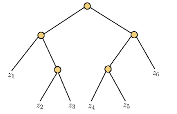
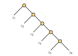
Figure 1: Graph representation of the hierarchical Tucker (HT) and tensor train (TT) decomposition of a six-dimensional function $f(z_{1},\ldots,z_{6})$.

Efficient algorithms to perform basic operations between hierarchical tensors, such as addition, orthogonalization, rank reduction, scalar products, multiplication, and linear transformations, are discussed in [54, 43, 51, 55]. Parallel implementations of such algorithms were recently proposed in [56, 57]. Methods for reducing the computational cost of tensor trains are discussed in [58, 59, 55]. Applications to the Vlasov kinetic equation can be found in [60, 61, 62].

3 Numerical Approximation of High-Dimensional PDEs

In this section we develop efficient numerical methods to integrate high-dimensional linear PDEs of the form

$$\frac{\partial f(\bm{z},t)}{\partial t}=L(\bm{z})f(\bm{z},t),$$ (17)

where $L(\bm{z})$ is a linear operator. The algorithms we propose are based on numerical tensor methods and appropriate rank-reduction techniques, such as hierarchical singular value decomposition [44, 57] and alternating least squares [31, 30]. To begin with, we assume that $L(\bm{z})$ is a separable linear operator with separation rank $r_{L}$, i.e., an operator of the form

$$L(\bm{z})=\sum_{l=1}^{r_{L}}\alpha_{l}L_{1}^{l}(z_{1})\cdots L_{N}^{l}(z_{N}).$$ (18)

For each $i$ and $j$, $L_{i}^{j}(z_{i})$ is a linear operator acting only on variable $z_{i}$. As an example, the operator

$$L(z_{1},z_{2})=z^{2}_{1}\frac{\partial}{\partial z_{1}}-\sin(z_{2})\frac{\partial^{2}}{\partial z_{1}\partial z_{2}}.$$ (19)

is separable with separation rank $r_{L}=2$ in dimension $N=2$. It can be written in the form (18) if we set $\alpha_{1}=\alpha_{2}=1$ and

$$L_{1}^{1}(z_{1})=z_{1}^{2}\frac{\partial}{\partial z_{1}},\quad L_{2}^{1}(z_{2})=1,\quad L_{1}^{2}(z_{1})=\frac{\partial}{\partial z_{1}},\quad L_{2}^{2}(z_{2})=-\sin(z_{2})\frac{\partial}{\partial z_{2}}.$$ (20)

3.1 Tensor Methods with Implicit Time Stepping

Let us discretize the PDE in (17) in time by using the Crank-Nicolson method. To this end, consider an evenly-spaced grid $t_{n}=n\Delta t$ ($n=0,1,...$) with time step $\Delta t$. This yields

$$\left[I-\frac{\Delta t}{2}L(\bm{z})\right]f_{n+1}(\bm{z})=\left[I+\frac{\Delta t}{2}L(\bm{z})\right]f_{n}(\bm{z})+\Delta t\tau_{n+1}(\bm{z}),$$ (21)

where $I$ is the identity matrix, $f_{n}(\bm{z})=f(\bm{z},t_{n})$, and $\tau_{n+1}(\bm{z})$ is the local truncation error of the Crank-Nicolson method at time $t_{n+1}$ [63]. Rewriting this in a more compact notation yields [23]

$$A(\bm{z})f_{n+1}(\bm{z})=B(\bm{z})f_{n}(\bm{z})+\Delta t\tau_{n+1}(\bm{z}),$$ (22)

where

$$A=I-\frac{\Delta t}{2}L(\bm{z}),\quad\textrm{and}\quad B=I+\frac{\Delta t}{2}L(\bm{z}).$$ (23)

It follows from the definition of $L(\bm{z})$ in (18) that both $A(\bm{z})$ and $B(\bm{z})$ are separable operators of the form

$$A=\sum_{q=0}^{r_{L}}\eta_{q}E^{q}_{1}(z_{1})\cdots E^{q}_{N}(z_{N}),\qquad B=\sum_{q=0}^{r_{L}}\zeta_{q}E^{q}_{1}(z_{1})\cdots E^{q}_{N}(a_{N}),$$ (24)

where $\eta_{0}=\zeta_{0}=1$, $E^{0}_{j}(z_{j})=1$ ($j=1,...,N$),

$$\eta_{j}=-\frac{\Delta t}{2},\qquad\zeta_{j}=-\eta_{j},\qquad E^{q}_{j}(z_{j})=L^{q}_{j}(z_{j}),\qquad q=1,...,r_{L},\quad j=1,...,N.$$ (25)

A substitution of the canonical tensor decomposition

$$\hat{f}_{n+1}(\bm{z})=\sum_{l=1}^{r}\prod_{k=1}^{N}G^{l}_{k}(z_{k},t_{n+1})$$ (27)

into (21) yields the residual

$$R(\bm{z},t_{n+1})=A(\bm{z})\hat{f}_{n+1}(\bm{z})-B(\bm{z})\hat{f}_{n}(\bm{z}),$$ (28)

in which the local truncation error $\Delta t\tau_{n+1}$ is embedded into $R(\bm{z},t_{n+1})$. Next, we minimize the residual using the alternating least squares algorithm, described in Section 3.1, to obtain the solution at time $t_{n+1}$. In particular, we look for a minimizer of (28) computed in a parsimonious way. The key idea again is to split the optimization problem

$$\min_{\beta_{ks}^{l}(t_{n+1})}\left\|R(\bm{z},t_{n+1})\right\|_{L_{2}}^{2}$$ (29)

into a sequence of optimization problems of smaller dimension, which are solved sequentially and in parallel [31] (see Appendix B). To this end, we define

$$\bm{\beta}_{k}(t_{n})=[\beta^{1}_{k1}(t_{n}),...,\beta^{1}_{kQ}(t_{n}),...,\beta^{r}_{k1}(t_{n}),...,\beta^{r}_{kQ}(t_{n})]^{T}\qquad k=1,...,N.$$ (30)

The vector $\bm{\beta}_{k}(t_{n})$ collects the degrees of freedom representing the solution functional along $z_{k}$ at time $t_{n}$, i.e., the set of functions $\{G_{k}^{1}(z_{k},t_{n}),...,G^{r}_{k}(z_{k},t_{n})\}$. Minimization of (29) with respect to independent variations of $\bm{\beta}_{k}(t_{n+1})$ yields a sequence of convex optimization problems (see Figure 2)

$$\min_{\bm{\beta}_{1}(t_{n+1})}\left\|R(\bm{z},t_{n+1})\right\|_{L_{2}}^{2},\quad\min_{\bm{\beta}_{2}(t_{n+1})}\left\|R(\bm{z},t_{n+1})\right\|_{L_{2}}^{2},\quad\cdots,\quad\min_{\bm{\beta}_{N}(t_{n+1})}\left\|R(\bm{z},t_{n+1})\right\|_{L_{2}}^{2}.$$ (31)

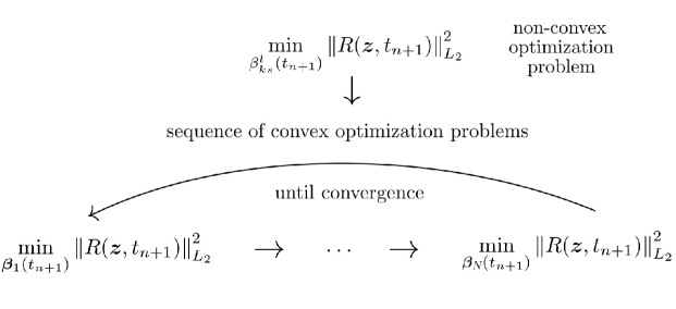
Figure 2: Sketch of the alternating least squares (ALS) algorithm for the minimization of the norm of the residual $R(\bm{z},t_{n+1})$ defined in equation (28).

This set of equations defines the alternating least-squares (ALS) method. The Euler-Lagrange equations, which identify stationary points of (31), are linear systems in the form

$$\bm{M}^{L}_{q}\bm{\beta}_{q}(t_{n+1})=\bm{M}^{R}_{q}\bm{\beta}_{q}(t_{n})\qquad q=1,...,N$$ (32)

where

$$\bm{M}^{L}_{q}=\sum_{e,z=0}^{r_{L}}K^{L}_{ez}\left[{\displaystyle\begin{subarray}{c}\vspace{0.2cm}\\ \vspace{0.04cm}N\\ \bigcirc\\ k=1\\ k\neq q\end{subarray}}\hat{\bm{\beta}}_{k}(t_{n+1})^{T}\bm{E}^{ez}_{k}\hat{\bm{\beta}}_{k}(t_{n+1})\right]^{T}\otimes\left[{\bm{E}}^{ez}_{q}\right]^{T},$$ (33)

$$\bm{M}^{R}_{q}=\sum_{e,z=0}^{r_{L}}{K}^{R}_{ez}\left[{\begin{subarray}{c}\vspace{0.2cm}\\ \vspace{0.04cm}N\\ \bigcirc\\ k=1\\ k\neq q\end{subarray}}\hat{\bm{\beta}}_{k}(t_{n})^{T}{\bm{E}}^{ez}_{k}\hat{\bm{\beta}}_{k}(t_{n+1})\right]^{T}\otimes\left[{\bm{E}}^{ez}_{q}\right]^{T},$$ (34)

and

$$\left[{\bm{E}}^{ez}_{q}\right]_{sh}=\int_{-b}^{b}E_{q}^{e}(a)\phi_{s}(a)E_{q}^{z}(a)\phi_{h}(a)\text{d}a.$$ (35)

In (33)–(34), $\bigcirc$ denotes the Hadamard matrix product, $\otimes$ is the Kronecker matrix product, $\hat{\bm{\beta}}_{k}$ is the matricization of $\bm{\beta}_{k}$, i.e.,

$$\hat{\bm{\beta}}_{k}(t_{n})=\left[\begin{array}[]{ccc}\beta^{1}_{k1}(t_{n})&\cdots&\beta^{r}_{k1}(t_{n})\\ \vdots&\ddots&\vdots\\ \beta^{1}_{kQ}(t_{n})&\cdots&\beta^{r}_{kQ}(t_{n})\end{array}\right],$$ (36)

$\bm{E}^{ez}_{q}$ are $Q\times Q$ matrices, and $K^{L}_{ez}$ and ${K}^{R}_{ez}$ are entries of the matrices

$$\bm{K}^{L}=\bm{\eta}\bm{\eta}^{T},\quad\textrm{and}\quad\bm{K}^{R}=\bm{\eta}\bm{\zeta}^{T},$$ (37)

where $\bm{\eta}$ and $\bm{\zeta}$ are column vectors with entries $\eta_{q}$ and $\zeta_{q}$ defined in (24). The ALS algorithm, combined with canonical tensor representations, effectively reduces evaluation of $N$-dimensional integrals to evaluation of the sum of products of one-dimensional integrals.

Summary of the Algorithm

Often many of the integrals in (35) only differ by a prefactor and in that case the number of unique integrals can be reduced to a very small number ($4$ in the case of the Boltzmann-BGK equation discussed in Section 4.2). Thus, it is convenient to precompute a map between such integrals and any entry in (35). Such a map allows us to rapidly compute each matrix $\bm{E}_{q}^{ez}$ in (33) and (34), and therefore to efficiently build the matrix system. Next, we compute the canonical tensor decomposition of the initial condition $f(\bm{z},0)$ by applying the methods described in Section 2.1. This yields the set of vectors $\{\bm{\beta}_{1}(t_{0}),...,\bm{\beta}_{N}(t_{0})\}$, from which the matrices $\bm{M}^{L}_{1}$ and $\bm{M}^{R}_{1}$ in (33) and (34) are built. To this end, we need an initial guess for $\{\bm{\beta}_{1}(t_{1}),...,\bm{\beta}_{N}(t_{1})\}$ given, e.g., by $\{\bm{\beta}_{1}(t_{0}),...,\bm{\beta}_{N}(t_{0})\}$ or its small random perturbation. With $\bm{M}^{L}_{1}$, $\bm{M}^{R}_{1}$ in place, we solve the linear system in (32) and update $\bm{\beta}_{1}(t_{1})$. Finally, we recompute $\bm{M}^{L}_{2}$ and $\bm{M}^{R}_{2}$ (with the updated $\bm{\beta}_{1}(t_{1})$) and solve for $\bm{\beta}_{2}(t_{1})$. This process is repeated for $q=3,\ldots,N$ and iterated among all the variables until convergence (see Figure 2). The ALS iterations are said to converge if

$$\left\|\bm{\beta}^{(j)}_{k}(t_{n})-\bm{\beta}^{(j-1)}_{k}(t_{n})\right\|_{2}^{2}\leq\epsilon_{\textrm{Tol}},\qquad j=1,\ldots,N_{\text{max}},$$ (38)

where $j$ here denotes the iteration number whose maximum value is $N_{\text{max}}$, and $\epsilon_{\textrm{Tol}}$ is a prescribed tolerance on the increment of such iterations. Parallel versions of the ALS algorithm associated with canonical tensor decompositions were recently proposed in [31, 40] (see also Appendix B). We emphasize that the use of a hierarchical tensor series instead of (27) (see Section (2.2)) also allows one to compute the unknown degrees of the expansion by using parallel ALS algorithms. This question was recently addressed in [56].

3.2 Tensor Methods with Explicit Time Stepping

Let us discretize PDE (17) in time by using any explicit time stepping scheme, for example the second-order Adams-Bashforth scheme [63]

$$f_{n+2}(\bm{z})=f_{n+1}(\bm{z})+\frac{\Delta t}{2}L(\bm{z})\left(3f_{n+1}(\bm{z})-f_{n}(\bm{z})\right)+\Delta t\tau_{n+2}(\bm{z}).$$ (39)

In this setting, the only operations needed to compute $f_{n+2}$ with tensor methods are: i) addition, ii) application of a (separable) linear operator $L$, and iii) rank reduction, the last operation being the most important among the three [43, 51, 33]. Rank reduction can be achieved, e.g., by hierarchical singular value decomposition [44, 57] or by alternating least squares [31].

From a computational perspective, it is useful to split the sequence of tensor operations yielding $f_{n+2}$ in (39) into simple tensor operations followed by rank reduction. For example, $L(3f_{n+1}-f_{n})$ might be evaluated as follows: i) compute $w_{n+1}=f_{n+1}-f_{n}$; ii) perform rank reduction on $w_{n+1}$; iii) compute $Lw_{n+1}$ and perform rank reduction again. This allows one to minimize the memory requirements and overall computational cost. Unfortunately, splitting tensor operations into sequences of tensor operations followed by rank reduction can produce severe cancellation errors. In some cases this problem can be mitigated. For example, an efficient and robust algorithm, which allows us to split sums and rank reduction operations, was recently proposed in [51] in the context of hierarchical Tucker formats. The algorithm leverages the block diagonal structure arising from addition of hierarchical Tucker tensors.

4 Numerical Results

In this section, we demonstrate the accuracy and effectiveness of the numerical tensor methods discussed above. Two case studies are considered: an advection equation in six dimensions plus time and the Boltzmann-BGK equation.

4.1 Advection Equation

Consider an initial-value problem

$$\frac{\partial f}{\partial t}+\sum_{j=1}^{N}\left(\sum_{k=1}^{N}C_{jk}z_{k}\right)\frac{\partial f}{\partial z_{j}}=0,\qquad f(z_{1},\ldots,z_{N},0)=f_{0}(z_{1},\ldots,z_{N}),$$ (40)

where $N$ is the number of independent variables forming the coordinate vector $\bm{z}=(z_{1},\ldots,z_{N})^{\top}$, and $C_{jk}$ are components of a given matrix of coefficients $\bm{C}$. The analytical solution to this initial-value problem is computed with the method of characteristics as [64]

$$f(\bm{z},t)=f_{0}\left(\text{e}^{-t\bm{C}}\bm{z}\right).$$ (41)

We choose the initial condition $f_{0}$ to be a fully separable product of exponentials,

$$f_{0}(\bm{z})=\text{e}^{-\left\|\bm{z}\right\|^{2}_{2}}.$$ (42)

The time dynamics of the solution (41)-(42) is entirely determined by the matrix $\bm{C}$. In particular, if $\bm{C}$ has eigenvalues with positive real part then the matrix exponential $\exp(-t\bm{C})$ is a contraction map. In this case, $f(\bm{z},t)\rightarrow 1$ as $t\rightarrow\infty$, at each point $\bm{z}\in\mathbb{R}^{N}$. Figure 3 exhibits the analytical solution (41) generated by a $2\times 2$ matrix $\bm{C}$, whose eigenvalues are complex conjugate with positive real part.

$t=0$                                                $t=3$                                                $t=6$

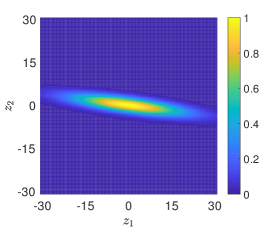
Figure 3: Solution to the multivariate PDE (40) in $N=2$ dimensions. The stable spiral at the origin of the characteristic system attracts every curve in the phase space and ultimately yields $f=1$ everywhere after a transient.

The side length of the hypercube cube that encloses any level set of the solution at time $t$ depends on the number of dimensions $N$. In particular, the side-length of the hypercube that encloses the set $\{\bm{z}\in\mathbb{R}^{N}\,|\,f(\bm{z},t)\geq\epsilon\}$ is given by

$$\frac{1}{2}\sqrt{\frac{-\log(\epsilon)}{N\lambda_{\text{min}}}}\leq b\leq\frac{1}{2}\sqrt{\frac{-\log(\epsilon)}{\lambda_{\text{min}}}}.$$ (43)

where $\lambda_{\text{min}}$ is the smallest eigenvalue of the matrix $\exp(t\bm{C})^{\top}\exp(t\bm{C})$. Equation (40) can be written in the form (17), with separable operator $L$ (separation rank $N^{2}$). Specifically, the one-dimensional operators $L^{l}_{j}(z_{j})$ appearing in (18) are explicitly defined in Table 1.

$q$	$\alpha_{q}$	$L_{1}^{q}$	$L_{2}^{q}$	$\cdots$	$L_{N}^{q}$
$1$	$-C_{11}$	$z_{1}\partial_{z_{1}}$	$1$	$\cdots$	$1$
$2$	$-C_{12}$	$\partial_{z_{1}}$	$z_{2}$	$\cdots$	$1$
$\vdots$	$\vdots$	$\vdots$	$\vdots$	$\vdots$	$\vdots$
$N$	$-C_{1N}$	$\partial_{z_{1}}$	$1$	$\cdots$	$z_{N}$
$N+1$	$-C_{21}$	$z_{1}$	$\partial_{z_{2}}$	$\cdots$	$1$
$N+2$	$-C_{22}$	$1$	$z_{2}\partial_{z_{2}}$	$\cdots$	$1$
$\vdots$	$\vdots$	$\vdots$	$\vdots$	$\vdots$	$\vdots$
$2N$	$-C_{2N}$	$1$	$\partial_{z_{2}}$	$\cdots$	$z_{N}$
$\vdots$	$\vdots$	$\vdots$	$\vdots$	$\vdots$	$\vdots$
$N^{2}-N+1$	$-C_{N1}$	$z_{1}$	$1$	$\cdots$	$\partial_{z_{N}}$
$N^{2}-N+2$	$-C_{N2}$	$1$	$z_{2}$	$\cdots$	$\partial_{z_{N}}$
$\vdots$	$\vdots$	$\vdots$	$\vdots$	$\vdots$	$\vdots$
$N^{2}$	$-C_{NN}$	$1$	$1$	$\cdots$	$z_{N}\partial_{z_{N}}$

Table 1: Advection equation (40). Ordering of the linear operators defined in (18).

We used tensor methods, both canonical tensor decomposition and hierarchical tensor methods, and explicit time stepping (Section 3.2) to solve numerically (40) in the periodic hypercube $[-60,60]^{N}$. Each tensor component was discretized by using a Fourier spectral expansion with $600$ nodes in each variable (e.g., basis functions in (2) or (14)). The accuracy of the numerical solution was quantified in terms of the time-dependent relative error

$$\epsilon_{m}(t)=\left|\frac{f(\bm{z}^{*},t)-\hat{f}(\bm{z}^{*},t)}{f(\bm{z}^{*},t)}\right|,$$ (44)

where $f$ is the analytical solution (41), $\hat{f}$ is the numerical solution obtained by using the canonical or hierarchical tensor methods with separation rank $r$.

       Canonical Tensor Method                           Hierarchical Tensor Method

two dimensions   

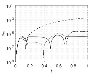
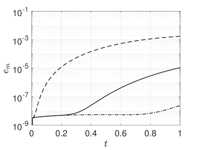
three dimensions   

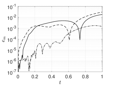
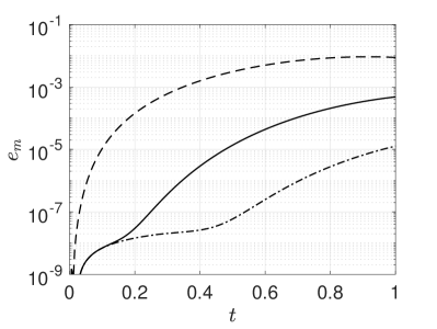
six dimensions   

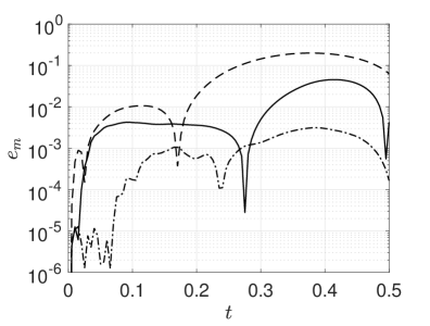
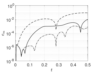
$--$ $r_{max}=4$          — $r_{max}=8$           $-\cdot-$ $r_{max}=12$

Figure 4: Advection equation (40). Relative pointwise error (44) for several values of the separation ranks $r$ and the number of independent variables $N$. These results are obtained by using the canonical and hierarchical tensor methods with explicit time stepping (see Section 3.2). The separation rank is computed adaptively at each time step up to the maximum value $r_{\text{max}}$.

Figure 4 shows the relative pointwise error (44), computed at $\bm{z}^{*}=(h,h,\ldots,h)$ with $h=0.698835274542439$, for different separation ranks $r$ and different number of independent variables $N$. As expected, the accuracy of the numerical solution increases with the separation rank $r$. Also, the relative error increases with the number of dimensions $N$. It is worthwhile emphasizing that the rank reduction in canonical tensor decomposition at each time step is based on a randomized algorithm that requires initialization at each time-step. This means that results of simulations with the same nominal parameters may be different. On the other hand, tensor methods based on a hierarchical singular value decomposition, such as the hierarchical Tucker decomposition [44, 57], do not suffer from this issue. The separation rank of both canonical and hierarchical tensor methods is computed adaptively up to the maximum value $r_{\text{max}}$ specified in the legend of Figure 4. In two dimensions, the CP-ALS algorithm yields the similar error plots for $r_{\text{max}}=8$ and $r_{\text{max}}=12$. This is because $r<8$ in both cases, and throughout the simulation up to $t=1$. The difference between these results is due to the random initialization required by the ALS algorithm at each time step.

4.2 Boltzmann-BGK Equation

In this section we develop an accurate ALS-based algorithm to solve a linearized BGK equation (see Appendix A for details of its derivation),

$$\frac{\partial f}{\partial t}+\bm{v}\cdot\nabla_{\bm{x}}f=\nu I,\qquad I=f_{\text{eq}}(\bm{v})-f.$$ (45)

Here, $f(\bm{z},t)$ is a probability density function is six phase variables plus time; the coordinate vector $\bm{z}=(\bm{x},\bm{v})^{\top}$ is composed of three spatial dimensions $\bm{x}=(x_{1},x_{2},x_{3})^{\top}$ and three components of the velocity vector $\bm{v}=(v_{1},v_{2},v_{3})^{\top}$; $f_{\text{eq}}$ denotes a locally Maxwellian distribution,

$$f_{\text{eq}}(\bm{v})=\frac{\rho}{(2\pi RT)^{3/2}}\exp\left(-\frac{\left\|\bm{v}\right\|_{2}^{2}}{2RT}\right),$$ (46)

with uniform gas density $\rho$, temperature $T$, and velocity $\bm{v}$; $R$ is the gas constant; and $\nu=\kappa\rho T^{1-\mu}$ with positive constants $\kappa$ and $\mu$. The solution to the linearized Boltzmann-BGK equation (47) is also computable analytically, which provides us with a benchmark solution to check the accuracy of our algorithms.

As before we start by rewriting this equation in an operator form,

$$\frac{\partial f}{\partial t}=Lf+C$$ (47)

where

$$L(\bm{x},\bm{v})=-\bm{v}\cdot\nabla_{\bm{x}}-\nu I,\qquad C(\bm{v})=\nu f_{\text{eq}}(\bm{v}).$$ (48)

Note that $L$ is a separable linear operator with separation rank $r_{L}=4$, which can be rewritten in the form

$$L(\bm{z})=\sum_{q=1}^{4}\alpha_{q}L^{q}_{1}(z_{1})\cdots L_{6}^{q}(z_{6}),$$ (49)

for suitable one-dimensional linear operators $L^{q}_{j}(a_{j})$ defined in Table 2. Similarly, $C(\bm{v})$ in (48) is separated as

$$C(\bm{v})=C_{1}(v_{1})C_{2}(v_{2})C_{3}(v_{3}),\quad\textrm{where}\quad C_{i}(v_{i})=\frac{(\nu\rho)^{1/3}}{(2\pi RT)^{1/2}}\exp\left(-\frac{v_{i}^{2}}{2RT}\right).$$ (50)

$q$	$\alpha_{q}$	$L_{1}^{q}$	$L_{2}^{q}$	$L_{3}^{q}$	$L_{4}^{q}$	$L_{5}^{q}$	$L_{6}^{q}$
$1$	$-\nu$	$1$	$1$	$1$	$1$	$1$	$1$
$2$	$-1$	$\partial/\partial x_{1}$	$1$	$1$	$v_{1}$	$1$	$1$
$3$	$-1$	$1$	$\partial/\partial x_{2}$	$1$	$1$	$v_{2}$	$1$
$4$	$-1$	$1$	$1$	$\partial/\partial x_{3}$	$1$	$1$	$v_{3}$

Table 2: Ordering of the linear operators defined in equation (49).

From a numerical viewpoint, the solution to (47) can be represented by using any of the tensor series expansion we discussed in Section 2. In particular, hereafter we develop an algorithm based on canonical tensor tensor decomposition, alternating least squares, and implicit time stepping (see Section (3.1)). To this end, we discretize (47) in time with the Crank-Nicolson method to obtain

$$\left[I-\frac{\Delta t}{2}L\right]f_{n+1}=\left[I+\frac{\Delta t}{2}L\right]f_{n}+\Delta tC+\Delta t\tau_{n},$$ (51)

where $f_{n}(\bm{z})=f(\bm{z},t_{n})$ and $\tau_{n}$ it the local truncation error of the Crank-Nicholson method at $t=t_{n}$ ([63], p. 499). This equation can be written in a compact notation as

$$Af_{n+1}=Bf_{n}+\Delta tC+\Delta t\tau_{n},$$ (52)

where $A$ and $B$ are separable operators in the form (24), where all quantities are defined in Table 3.

$q$	$\eta_{q}$	$\zeta_{q}$	$E_{1}^{q}$	$E_{2}^{q}$	$E_{3}^{q}$	$E_{4}^{q}$	$E_{5}^{q}$	$E_{6}^{q}$
$1$	$\nu(1+\Delta t/2)$	$\nu(1-\Delta t/2)$	$1$	$1$	$1$	$1$	$1$	$1$
$1$	$\Delta t/2$	$-\Delta t/2$	$\partial/\partial x_{1}$	$1$	$1$	$v_{1}$	$1$	$1$
$1$	$\Delta t/2$	$-\Delta t/2$	$1$	$\partial/\partial x_{2}$	$1$	$1$	$v_{2}$	$1$
$1$	$\Delta t/2$	$-\Delta t/2$	$1$	$1$	$\partial/\partial x_{3}$	$1$	$1$	$v_{3}$

Table 3: Ordering of the linear operators $A$ and $B$ defined in (24).

A substitution of the canonical tensor decomposition

$$\hat{f}_{n+1}=\sum_{l=1}^{r}\prod_{k=1}^{6}G^{l}_{k}(z_{k},t_{n+1})$$ (54)

into equation (21) yields the residual

$$R(\bm{z},t_{n+1})=A(\bm{z})\hat{f}_{n+1}(\bm{z})-B(\bm{z})\hat{f}_{n}(\bm{z})+\Delta tC(z_{4},z_{5},z_{6}),$$ (55)

which can be minimized by using the alternating least squares method, as we described in Section 3.1 to obtain the solution at time $t_{n+1}$.

Nonlinear Boltzmann-BGK Model

The numerical tensor methods we discussed in Section 3.1 and Section 3.2 can be extended to compute the numerical solution of the fully nonlinear Boltzmann-BGK model

$$\frac{\partial f}{\partial t}+\bm{v}\cdot\nabla_{\bm{x}}f=\nu(\bm{x},t)\left(f_{eq}(\bm{x},\bm{v},t)-f(\bm{x},\bm{v},t)\right).$$ (56)

Here, $f_{eq}(\bm{x},\bm{v},t)$ is the equilibrium distribution (70), while the collision frequency $\nu(\bm{x},t)$ can can be expressed, e.g., as in (76). From a mathematical viewpoint both quantities $f_{eq}$ and $\nu$ are nonlinear functionals of the PDF $f(\bm{x},\bm{v},t)$ (see equations (71)-(73)). Therefore (56) is an advection equation driven driven by a nonlinear functional of $f(\bm{x},\bm{v},t)$. The evaluation of the integrals appearing in (71)-(73) poses no great challenge if we represent $f$ as a canonical tensor (1) or as a hierarchical Tucker tensor (14). Indeed, such integrals can be factored as sums of product of one-dimensional integrals in a tensor representation. Moreover, computing the inverse of $\rho(\bm{x},t)$ in (72) and (73) is relatively simple in a collocation setting. In fact, we just need to evaluate the full tensor $\rho(\bm{x},t)$, on a three-dimensional tensor product grid and compute $1/\rho(\bm{x},t)$ pointwise. If needed, we could then compute the tensor decomposition of $1/\rho(x,t)$, e.g., by using the canonical tensor representations and the ALS algorithm we discussed in Section 2.1. This allows us to evaluate the BGK collision operator and represent it in a tensor series expansion. The solution to the Boltzmann BGK equation can be then computed by operator splitting methods [65, 66].

Initial and Boundary conditions

To validate the proposed alternating least squares algorithm we set the initial condition to be either coincident with the homogeneous Maxwell-Boltzmann distribution (46), i.e.,

$$f\left(\bm{x},\bm{v},0\right)=\frac{\rho}{\left(2\pi RT\right)^{3/2}}\exp\left(-\frac{\left\|\bm{v}\right\|_{2}^{2}}{2RT}\right)$$ (57)

or a slight perturbation of it. The PDF (57) is obviously separable with separation rank one. Moreover, we set the computational domain to be a the periodic hyperrectangle $[-b_{x},b_{x}]^{3}\times[-b_{v},b_{v}]^{3}$. It is essential that such domain is chosen large enough to accommodate the support of the PDF at all times, thus preventing physically unrealistic correlations between the distribution function. More generally, it is possible to enforce other types of boundary conditions by using appropriate trial functions, or by a mixed approach [67, 68, 69] in the case of Maxwell boundaries.

Unless otherwise stated, all simulation parameters are set as in Table 4. Such setting corresponds to the problem of computing the dynamics of Argon within the periodic hyperrectangle $[-b_{x},b_{x}]^{3}\times[-b_{v},b_{v}]^{3}$. We are interested in testing our algorithms in two different regimes: i) steady state, and ii) relaxation to statistical equilibrium.

Parameter	Symbol	value
Temperature	$T$	$300\,$\mathrm{K}$$
Number density	$n$	$2.4143\cdot 10^{25}\,$\mathrm{m}^{-3}$$
Specific gas constant	$R$	$208\,$\mathrm{J}\,\mathrm{k}\mathrm{g}^{-1}\,\mathrm{K}^{-1}$$
Relaxation time	$\tau_{R}$	$0.40034\,$\mathrm{s}$$
Collision frequency	$\nu$	$1/\tau_{R}$
Position domain size	$b_{x}$	$500\,$\mathrm{m}$$
Velocity domain size	$b_{v}$	$5\sqrt{R_{S}T}$
Time step	$\Delta t$	$0.01\tau_{R}$
Number of iterations	$N_{\text{Iter}}$	$1000$
ALS tolerance	$\epsilon_{\text{Tol}}$	$10^{-8}$
Series truncation	$Q$	$11$

Table 4: Simulation parameters we employed in the numerical approximation of the Boltzmann-BGK model. These parameters correspond to a kinetic simulation of dynamics of Argon in the periodic hyperrectangle $[-b_{x},b_{x}]^{3}\times[-b_{v},b_{v}]^{3}$. The time step in the implicit Crank-Nicolson method is $\Delta t$, while the tolerance in the ALS iterations at each time step is $\epsilon_{\text{Tol}}$.

4.2.1 Canonical Tensor Decomposition of the Maxwell-Boltzmann Distribution

We begin with a preliminary convergence study of the canonical tensor decomposition (1) applied to the one-particle Maxwell distribution $f_{eq}(\bm{v})$. Such study allows us to identify the size of the hyperrectangle that includes the support of the Maxwellian equilibrium distribution. This is done in Figure 5, where we plot the tensor expansion of $f_{eq}(\bm{v})$ as function of the non-dimensional molecular speed $\left\|\bm{v}\right\|_{2}/\sqrt{R_{S}T}$, for different number of basis functions $Q$ in (2), and for various values of the dimensionless velocity domain size $b_{v}/\sqrt{RT}$. It is seen that for small values of $b_{v}/\sqrt{RT}$, a small number of basis functions $Q$ is sufficient to capture the exact equilibrium distribution. At the same however, small values of $b_{v}/\sqrt{RT}$ result in distribution functions with truncated tails, as can be seen in Figures 5 (a), 5 (b), and 5 (e). Figures 5 (c) and 5 (g) demonstrate that the dimensionless velocity domain size $b_{v}/\sqrt{RT}=5$ is sufficient to avoid truncation of the tail of the distribution, and that a series expansion with $Q=11$ in each variable is sufficient to accurately capture the equilibrium distribution. This justifies the choice of parameters in Table (4).

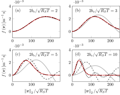
(a)

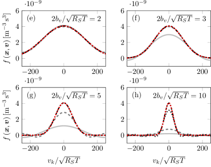
(b)

Figure 5: One-particle Maxwell-Boltzmann distribution $f_{eq}(\bm{v})$ () as a function of the dimensionless molecular speed $\left\|\bm{v}\right\|_{2}/\sqrt{RT}$ for different dimensionless domain sizes $b_{v}/\sqrt{RT}$. In each case, we demonstrate convergence of the canonical tensor decomposition (1) of $f_{eq}$ as we increase the number of basis functions $Q$. Specifically, we plot the cases: $Q=3$ (), $Q=5$ (), $Q=11$ () and $Q=19$ ().

A more detailed analysis of the effects of the truncation order $Q$ and the dimensionless velocity domain size $b_{v}/\sqrt{RT}$ on the approximation error in $f_{eq}$ is done in Figure 6(a), where we plot the Normalized Mean Absolute Error (NMAE) versus $b_{v}/\sqrt{RT}$ and $Q$. The NMAE between two vectors $\bm{X}$ and $\bm{Y}$ of size $N$ is defined as:

$$\text{NMAE}=\frac{1}{N}\frac{\left\|\bm{X}-\bm{Y}\right\|_{1}}{\max{(\bm{X})}-\min{(\bm{Y})}},$$ (58)

where $\left\|\cdot\right\|_{1}$ is the standard vector 1-norm. In Figure 6(b) we plot the NMAE as a function of $Q\sqrt{RT}/b_{v}$. This results in a collapse of the data which suggests that if one wants to double the non-dimensional velocity domain size while maintaining the same accuracy, the series truncation order $Q$ needs to be doubled as well. In addition, it can be seen that starting at $Q\sqrt{RT}/b_{v}\approx 1$ the error decays rapidly with increasing $Q\sqrt{RT}/b_{v}$.

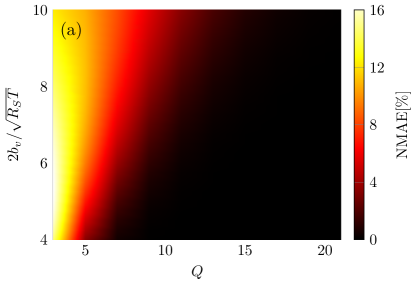
(a)

(b)

Figure 6: (a) Normalized Mean Absolute Error (NMAE) (58) between the analytical and the canonical tensor series expansion of the Maxwell-Boltzmann equilibrium distribution versus versus $Q$ and the dimensionless velocity domain size $b_{v}/\sqrt{RT}$. In Figure (b) we plot the NMAE in a log-log scale as function of $Q\sqrt{RT}/b_{v}$. We emphasize that the range of $Q$ and $b_{v}/\sqrt{RT}$ is the same in both Figures.

4.2.2 Steady State Simulations

We first test the the Boltzmann-BGK solver we developed in Section (3.1) on an initial value problem where the initial condition is set to be the Maxwell-Boltzmann distribution $f_{eq}(\bm{v})$ (see equation (46)). A properly working algorithm should keep such equilibrium distribution unchanged as the simulation progresses. In Figure 7 we plot the distribution of molecular velocities $f(\bm{v},t)$ as function of the molecular speed $\left\|\bm{v}\right\|_{2}\left|{\bm{\xi}}\right|$ at various dimensionless times $t/\tau_{R}$, where $\tau_{R}$ is the relaxation time in Table 4. It is seen that the alternating least squares algorithm we developed in Section (3.1) has a stable fixed point at the Maxwell-Boltzmann equilibrium distribution $f_{eq}$. This is an important test, as convergence of alternating least square is, in general, not granted for arbitrary residuals (see, e.g., [35, 70]).

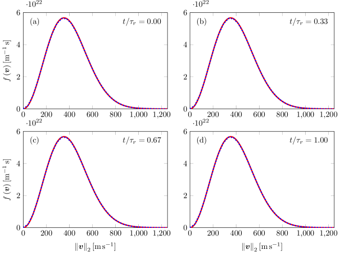
Figure 7: Solution to the Boltzmann-BGK equation (45) at different dimensionless times $t/\tau_{R}$ ($\tau_{R}$ is the relaxation time in Table 4). Specifically, we plot the Maxwell-Boltzmann equilibrium distribution (), its canonical tensor decomposition with $Q=11$ modes, and its the time evolution with the ALS algorithm we described in Section 3.1 (). It is seen that ALS has a stable fixed point at $f_{eq}(\bm{v})$. This is an important test as, in general, ALS iterations are not granted to converge (e.g., [35]).

We also computed the moments of the distribution function $f(\bm{x},\bm{v},t)$ at different times to verify whether ALS iterations preserve (density), momentum (velocity), and kinetic energy (temperature). In particular, we computed

$$\left<\rho\right>(t) =\frac{1}{b_{x}^{3}}\int_{-b_{x}}^{b_{x}}\cdots\int_{-b_{v}}^{b_{v}}f\left(\bm{x},\bm{v},t\right)d\bm{x}d\bm{v}$$ (59)

$$\left<\bm{u}\right>(t) =\frac{1}{\left<\rho\right>b_{r}^{3}}\int_{-b_{x}}^{b_{x}}\cdots\int_{-b_{v}}^{b_{v}}\bm{v}f\left(\bm{x},\bm{v},t\right)d\bm{x}d\bm{v},\quad\text{ and }$$ (60)

$$\left<T\right>(t) =\frac{1}{\left<\rho\right>b_{x}^{3}R_{S}}\int_{-b_{x}}^{b_{x}}\cdots\int_{-b_{v}}^{b_{v}}\left\|\bm{v}-\left<\bm{u}\right>\right\|_{2}^{2}f\left(\bm{x},\bm{v},t\right)d\bm{x}d\bm{v}$$ (61)

In Figure 8 we plot(59)-(61) versus time. It is seen that such quantities are indeed constants, i.e., ALS iterations preserve the average density, velocity and temperature.

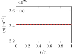
(a)

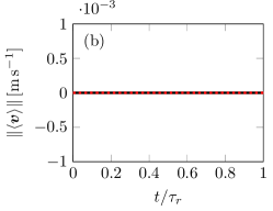
(b)

(c)

Figure 8: Average density $\left<\rho\right>(t)$, absolute average velocity $\left\|\left<u\right>\right\|_{2}$, and average temperature $\left<T\right>$ as function of the dimensionless time $t/\tau_{R}$: simulation results (); results at equilibrium (). The simulation results are obtained by setting the initial condition in (45) equal to the Maxwell-Boltzmann equilibrium distribution $f_{eq}$ and solving the Boltzmann-BGK model with the ALS algorithm described in Section 3.1. Clearly, ALS iterations preserve the average density, velocity and temperature.

4.2.3 Relaxation to Statistical Equilibrium

In this section we consider relaxation statistical equilibrium in the linearized Boltzmann-BGK model (45). This allows us to study the accuracy and computational efficiency of the proposed ALS algorithm in transient dynamics. To this end, we consider the initial condition

$$f\left(\bm{x},\bm{v},0\right)=f_{eq}\left(1+\epsilon\prod_{k=1}^{3}\cos\left(2\pi\frac{x_{k}}{b_{x}}\right)\right)$$ (62)

with $\epsilon=0.3$. Such initial condition is a slight perturbation of the Maxwell-Boltzmann equilibrium distribution (see Figure 9(a)). The simulation results we obtain are shown in Figures 9(b)-(d), where we plot the time evolution of the marginal PDF $f(\bm{v},t)$ versus the dimensionless time $t/\tau_{R}$. It is seen that the initial condition (62) is in the basin of attraction of $f_{eq}$, i.e., the ALS algorithm sends $f\left(\bm{x},\bm{v},0\right)$ into $f_{eq}\left(\bm{v}\right)$ after a transient. Moreover, $f(\bm{v},t)$ is attracted by $f_{eq}(\bm{v})$ exponentially fast in time at a rate $\tau_{R}=1/\nu$ (see Figure 11), consistently with results of perturbation analysis.

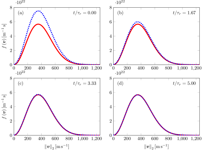
Figure 9: Relaxation to statistical equilibrium in the linearized Boltzmann-BGK model (45). Shown are time snapshots of the marginal PDF $p(\bm{v},t)$ we obtain by using the parallel ALS algorithm we proposed in Section 3.1 (). Note that the initial condition $f(\bm{v},0)$ is a slight perturbation of the Maxwell-Boltzmann distribution (). Note that $f(\bm{v},t)$ converges to $f_{eq}(\bm{v})$ exponentially fast in time (see Figure 11), consistently with results of perturbation analysis.

In Figure 10 we demonstrate that the parallel ALS algorithm we developed conserves the average density of particle, velocity (momentum) and temperature throughout the transient that yields statistical equilibrium.

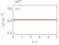
(a)

(b)

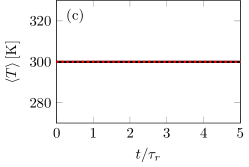
(c)

Figure 10: Conservation of the average density $\left<\rho\right>$, absolute average velocity $\left\|\left<\bm{v}\right>\right\|_{2}$, and average temperature $\left<T\right>$ during relaxation to statistical equilibrium. Shown are results obtained by using the parallel ALS algorithm we developed in Section 3.1 (), and the equilibrium initial values ().

In Figure 11 we plot the the Normalized Mean Absolute Error (NMAE) between the Maxwell-Boltzmann distribution $f_{eq}(\bm{v})$ and the distribution we computed numerically by using the proposed ALS algorithm. Specifically we plot NMAE versus the dimensionless time $t/\tau_{R}$ for different time-steps $\Delta t$ we employed in our simulations. The goal of such study is to assess the sensitivity of parallel ALS iterations on the time step $\Delta t$, and in turn on the total number of steps for a fixed integration time $T=5\tau_{R}$. Results of Figure 11 demonstrate that the decay of the distribution function $f(\bm{x},\bm{v},t)$ to the its equilibrium state is indeed exponential. Moreover, we see that the ALS algorithm is robust to $\Delta t$, which implies that the such algorithm is not sensitive to the total number of time steps we consider within a fixed integration time.

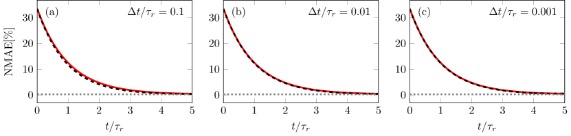
Figure 11: Relaxation to statistical equilibrium. Normalized Mean Absolute Error (NMAE) between the Maxwell-Boltzmann distribution $f_{eq}(\bm{v})$ and the numerical solution we obtain with the parallel ALS algorithm we proposed in Section 3.1 (). We also plot the theoretically predicted exponential decay (), and the best approximation error that we obtained based on approximating the equilibrium distribution $f_{eq}$ with a canonical tensor decomposition (1) with $Q=11$ modes (), $Q=11$ being the number of modes employed in the transient simulation.

Finally, we’d like to address scalability of the parallel ALS algorithm we developed in (B)., i.e., performance relative to the number of degrees of freedom and number of CPUs. To this end, we analyze here a few test cases we ran on a small workstation with 4 CPUs. The initial condition is set as $f_{eq}$ in all cases and we integrated the Boltzmann-BGK model (45) for $1000$ steps, with $\Delta t=0.01\tau_{R}$. The separation rank of the solution PDF is set to $r=1$ (see equation (1)). In Figure 12 (a) we plot the wall time $t_{\text{wall}}$ versus the total number of degrees of freedom of the ALS algorithm, i.e. $6Qr$. The plot shows that a typical simulation of the Boltzmann-BGK model in 6 dimensions with $r=1$ and $Q=11$ takes about $t_{\text{wall}}\approx 80$\min$$ on a single core to complete a simulation up $t=10\,$\mathrm{s}$$. With such value of $Q$ there is an error of only $0.5\%$ compared to the analytical Maxwell-Boltzmann distribution function. The total wall time scales with the power $5/2$ relative to number of degrees of freedom $6Qr$. In Figure 12 we show that the total wall time scales we obtain with the proposed parallel ALS algorithm scales almost linearly with the number of CPUs (power $-4/5$). The leveling off of performance for $4$ cores can be attributed to the fact that the desktop computer we employed for our simulations is optimized for inter-core communication. We expect better scaling performance of our ALS algorithm in computer clusters with infinity band inter-core communication.

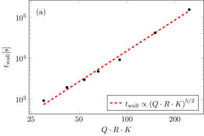
(a)

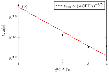
(b)

Figure 12: Wall time $t_{\text{wall}}$ versus the number of degrees of freedom of the ALS simulation (a), and versus the number CPUs (b).

5 Summary

In this paper we presented new parallel algorithms to solve high-dimensional partial differential equations based on numerical tensor methods. In particular, we studied canonical and hierarchical tensor expansions combined with alternating least squares and high-order singular value decomposition. Both implicit and explicit time integration methods were presented and discussed. We demonstrated the accuracy and computational efficiency of the proposed methods in simulating the transient dynamics generated by a linear advection equation in six dimensions plus time, and the well-known Boltzmann-BGK equation. We found that the algorithms we developed are extremely fast and accurate, even in a naive Matlab implementation. Unlike direct simulation Monte Carlo (DSMC), the high accuracy of the numerical tensor methods we propose makes it suitable for studying transient problems. On the other hand, given the nature of the numerical tensor discretization, implementation of the proposed algorithms to complex domains is not straightforward.

A Boltzmann Equation and its Approximations

In the classical kinetic theory of rarefied gas dynamics, the gas flow is described in terms of a non-negative density function $f(\bm{x},\bm{v},t)$ which provides the number of gas particles at time $t$ with velocity $\bm{v}\in\mathbb{R}^{3}$ at position $\bm{x}\in\mathbb{R}^{3}$. The density function $f$ satisfies the Boltzmann equation [71, 72, 65]. In the absence of external forces, such equation can be written as

$$\frac{\partial f}{\partial t}+\bm{v}\cdot\nabla_{\bm{x}}f=Q(f,f),$$ (63)

where $Q(f,f)$ is the collision integral describing the effects of internal forces due to particle interactions. From a mathematical viewpoint the collision integral is a functional of the particle density. Its form depends on the microscopic dynamics. For example, for classical rarefied gas flows [71, 73],

$$Q(f,f)(\bm{x},\bm{v},t)=\int_{\mathbb{R}^{3}}\int_{\mathbb{S}^{2}}B(\bm{v},\bm{v}_{1},\bm{\omega})\left|f(\bm{x},\bm{v}^{\prime},t)f(\bm{x},\bm{v}_{1}^{\prime},t)-f(\bm{x},\bm{v},t)f(\bm{x},\bm{v}_{1},t)\right|\text{d}\bm{\omega}\text{d}\bm{v}_{1}.$$ (64)

In this expression,

$$\bm{v}^{\prime}=\frac{1}{2}\left(\bm{v}+\bm{v}_{1}+\left\|\bm{v}-\bm{v}_{1}\right\|_{2}\bm{w}\right),\qquad\bm{v}_{1}^{\prime}=\frac{1}{2}\left(\bm{v}+\bm{v}_{1}-\left\|\bm{v}-\bm{v}_{1}\right\|_{2}\bm{w}\right)$$ (65)

and $\{\bm{v},\bm{v}_{1}\}$ represent, respectively, the velocities of two particles before and after the collision, $\bm{\omega}$ is a vector on the unit sphere $\mathbb{S}^{2}$, and $B(\bm{v},\bm{v}_{1},\bm{\omega})$ is the collision kernel. Such kernel is a non-negative function depending on the (Euclidean) norm $\left\|v-v_{1}\right\|_{2}$ and on the scattering angle $\theta$ between the relative velocities before and after the collision

$$\cos(\theta)=\frac{(\bm{v}-\bm{v}_{1})\cdot\bm{\omega}}{\left\|\bm{v}-\bm{v}_{1}\right\|_{2}}.$$ (66)

Thus, $B(\bm{v},\bm{v}_{1},\bm{\omega})$ becomes

$$B(\bm{v},\bm{v}_{1},\bm{\omega})=\left\|\bm{v}-\bm{v}_{1}\right\|_{2}\sigma\left(\left\|\bm{v}-\bm{v}_{1}\right\|_{2},\cos(\theta)\right),$$ (67)

$\sigma$ being the scattering cross section function [73]. The collision operator (64) satisfies a system of conservation laws in the form

$$\int_{\mathbb{R}^{3}}Q(f,f)(\bm{x},\bm{v},t)\psi(\bm{v})\text{d}\bm{v}=0,$$ (68)

where $\psi(\bm{v})$ is either $\{1,\bm{v},\left\|\bm{v}\right\|_{2}^{2}\}$. This yields, respectively, conservation of mass, momentum and energy. Moreover, $Q(f,f)$ satisfies the Boltzmann $H$-theorem

$$\int_{\mathbb{R}^{3}}Q(f,f)(\bm{x},\bm{v},t)\log\left(f(\bm{x},\bm{v},t)\right)\text{d}\bm{v}\leq 0$$ (69)

Such theorem implies that any equilibrium distribution function, i.e. any function $f$ for which $Q(f,f)=0$, has the form of a locally Maxwellian distribution

$$f_{\text{eq}}(\bm{x},\bm{v},t)=\frac{\rho(\bm{x},t)}{(2\pi RT(\bm{x},t))^{3/2}}\exp\left(-\frac{\left\|\bm{u}(\bm{x},t)-\bm{v}\right\|_{2}^{2}}{2RT(\bm{x},t)}\right),$$ (70)

where $R$ is the gas constant, and $\rho(\bm{x},t)$, $\bm{u}(\bm{x},t)$ and $T(\bm{x},t)$ are the density, mean velocity and temperature of the gas, defined as

$$\rho(\bm{x},t)= \int_{\mathbb{R}^{3}}f(\bm{x},\bm{v},t)d\bm{v},$$ (71)

$$\bm{u}(\bm{x},t)= \frac{1}{\rho(\bm{x},t)}\int_{\mathbb{R}^{3}}\bm{v}f(\bm{x},\bm{v},t)d\bm{v},$$ (72)

$$T(\bm{x},t)= \frac{1}{3\rho(\bm{x},t)}\int_{\mathbb{R}^{3}}\left\|\bm{u}(\bm{x},t)-\bm{v}\right\|_{2}^{2}f(\bm{x},\bm{v},t)d\bm{v}.$$ (73)

From a mathematical viewpoint, the Boltzmann equation (63) is a nonlinear integro-differential equation for a positive scalar field in six dimensions plus time. By taking suitable averages over small volumes in position space, it can be shown that the Boltzmann equation is consistent with the compressible Euler’s equations [74, 75], and the Navier-Stokes equations [76, 77, 78].

BGK Approximation

The simplest collision operator satisfying the conservation law (68) and the condition

$$Q(f,f)=0\Leftrightarrow f(\bm{x},\bm{v},t)=f_{\text{eq}}(\bm{x},\bm{v},t)$$ (74)

(see equation (70)) was proposed by Bhatnagar, Gross and Krook in [79]. The corresponding model, which is known as the BGK model, is defined by the linear relaxation operator

$$Q(f,f)=\nu(\bm{x},t)\left[f_{\text{eq}}(\bm{x},\bm{v},t)-f(\bm{x},\bm{v},t)\right]\qquad\nu(\bm{x},t)>0.$$ (75)

The field $\nu$ is usually set to be proportional to the density and the temperature of the gas [80]

$$\nu(\bm{x},t)=\kappa\rho(\bm{x},t)T(\bm{x},t)^{1-\mu}.$$ (76)

It can be shown that the Boltzmann-BGK model (75) converges to the correct Euler equations of incompressible fluid dynamics with the scaling $\bm{x}^{\prime}=\epsilon\bm{x}$, $t^{\prime}=\epsilon t$, and in the limit $\epsilon\rightarrow 0$. However, the model does not converge to the correct Navier-Stokes limit. The main reason is that it predicts an unphysical Prandtl number [81], which is larger that one obtained with the full collision operator (64). The correct Navier-Stokes limit can be recovered by more sophisticated BGK-type models, e.g., the ellipsoidal statistical BGK model [82].

Following [83, 84, 85, 86], we introduce additional simplifications, namely we assume that $\nu(\bm{x},t)=\nu$ is constant and assume the equilibrium density, temperature and velocity to be homogeneous across the spatial domain. Assuming $\bm{u}(\bm{x},t)=\bm{0}$, this yields an equilibrium distribution in (46). The last assumption effectively decouples the BGK collision operator from the probability density function $f(\bm{x},\bm{v},t)$. This, in turn, makes the BGK approximation linear, i.e., a six-dimensional PDE (45). Using both the isothermal assumption $T(\bm{x},t)=T$ [79], and constant density assumption $\rho(\bm{x},t)=\rho$ [84, 85, 86] means that our code can only be used to obtain solutions which are small perturbations from the equilibrium distribution. The term $\nu\left[f_{\text{eq}}(\bm{v})-f\right]$ in (45) represents the relaxation time approximation of the Boltzmann equation, $\nu$ is the collision frequency, here assumed to be homogeneous.

B Parallelization of the ALS Algorithm for the Boltzmann-BGK Equation

In this appendix we describe the parallel alternating least squares algorithms we developed to solve the linearized Boltzmann-BGK equation (45). Algorithm 1 shows the main Alternating Least Square (ALS) routine while algorithm 2, 3, 4, and 5 show the different subroutines. Each time step, $n$, the value of $\beta_{\text{Old}}$ is updated and then $\beta_{\text{New}}$ is determined in an iterative manner. Both the computations of the matrices $M_{k}$ and the vectors $\gamma_{k}$, as well as the calculation of the vectors $\beta_{\text{New},k}$ can be performed independently of each other, and thus can be easily parallelized. The current implementation assigns one core per dimension, but further optimization could be possible by implementing a parallel method to determine $\beta_{\text{New}}$ [87].

Algorithm 1 Parallel Alternating Least Squares (ALS) algorithm

1:procedure Main

2:     Initialization $\triangleright$ Load variables and allocate matrices

3:     $\beta_{\text{New}}=\beta_{0}$ $\triangleright$ Set initial condition

4:     for $N\leftarrow 1:N_{\text{Iter}}$ do

5:         $\epsilon_{\text{Conv}}\leftarrow\epsilon_{\text{Tol}}+1$ $\triangleright$ Reset convergence condition

6:         $\beta_{\text{Old}}\leftarrow\beta_{\text{New}}$

7:         while $\epsilon_{\text{Conv}}>\epsilon_{\text{Tol}}$ do

8:              $\beta_{\text{Int}}\leftarrow\beta_{\text{New}}$

9:              parfor $k\leftarrow 1:K$ do $\triangleright$ This for loop is executed in parallel

10:                  $\hphantom{M_{k}}\mathllap{M_{k}}\leftarrow\textsc{CreateMatrixM }(\beta_{\text{New},k},k)$

11:                  $\hphantom{M_{k}}\mathllap{\gamma_{k}}\leftarrow\textsc{CreateVectorGamma}(\beta_{\text{New},k},\beta_{\text{Old},k},k)$               

12:              parfor $k\leftarrow 1:K$ do $\triangleright$ This for loop is executed in parallel

13:                  $\beta_{\text{New},k}\leftarrow\textsc{ComputeBeta}(M_{k},\beta_{\text{New},k},\gamma_{k})$ $\triangleright$ Compute updated $\beta_{\text{New}}$               

14:              $\epsilon_{\text{Conv}}\leftarrow\textsc{ComputeConvergence}(\beta_{\text{Int}},\beta_{\text{New}})$ $\triangleright$ Update convergence condition

15:              $\beta_{\text{New}}\leftarrow\beta_{\text{Int}}+\left(\beta_{\text{New}}-\beta_{\text{Int}}\right)/4$ $\triangleright$ Update $\beta_{\text{New}}$               

16:end procedure

At each time step the CreateMatrixM subroutine (algorithm 2) updates the different elements of matrix $M_{k}$ for every iteration until convergence has been reached. The algorithm iterates over every element of the matrix and performs the multiplication and summation of the elements of $\hat{M}$. All the integrals were performed analytically and the results are stored in the map $\text{M}\left(k,l,z,s,q\right)$. Using this approach delivers significant savings in the computational cost of updating the matrix every iteration.

Algorithm 2 ALS Subroutines: CreateMatrixM

1:function CreateMatrixM($\beta_{\text{New},k},k$)

2:     for $l\leftarrow 1:R_{G}$ do $\triangleright$ Loop over all elements of $M_{k}$

3:         for $z\leftarrow 1:R_{G}$ do

4:              for $s\leftarrow-\left|{Q}\right|/2:\left|{Q}\right|/2$ do

5:                  for $q\leftarrow-\left|{Q}\right|/2:\left|{Q}\right|/2$ do

6:                       for $k^{\prime}\leftarrow 1:K$ do $\triangleright$ Loop over all elements of $\hat{M}$ for each element of $M_{k}$

7:                           for $\eta\leftarrow 1:r_{A}$ do

8:                                for $\upsilon\leftarrow 1:r_{A}$ do

9:                                    $j\leftarrow\left(\eta-1\right)r_{A}+\upsilon$

10:                                    if k’ = k then

11:                                         $\hat{M}_{k^{\prime},j}\leftarrow\textsc{M}(k^{\prime},\eta,\upsilon,s,q)$

12:                                    else

13:                                         $\hat{M}_{k^{\prime},j}\leftarrow 0$

14:                                         for $s^{\prime}\leftarrow-\left|{Q}\right|/2:\left|{Q}\right|/2$ do

15:                                             for $q^{\prime}\leftarrow-\left|{Q}\right|/2:\left|{Q}\right|/2$ do

16:                                                  $\hat{M}_{k^{\prime},j}\leftarrow\hat{M}_{k^{\prime},j}+\beta_{\text{New},k^{\prime},\left(l-1\right)Q+s^{\prime}}\beta_{\text{New},k^{\prime},\left(z-1\right)Q+q^{\prime}}\textsc{M}(k^{\prime},\eta,\upsilon,s^{\prime},q^{\prime})$                                                                                                                                                                                                             

17:                       $M_{k,\left(z-1\right)Q+q,\left(l-1\right)Q+s}\leftarrow\sum_{j=1}^{r_{A}^{2}}\prod_{k^{\prime}=1}^{K}\hat{M}_{k^{\prime},j}$ $\triangleright$ Fill matrix $M_{k}$                                               

18:     return $M_{k}$

19:end function

The subroutine CreateVectorGamma (algorithm 3) updates the vector $\gamma_{k}$. Similarly to the subroutine for the creation of matrix $M_{k}$ this algorithm iterates over all elements of the vector, and fills each of them using the values of $\beta_{\text{New}}$ and $\beta_{\text{Old}}$, and pre-calculated maps.

Algorithm 3 ALS Subroutines: CreateVectorGamma

1:function CreateVectorGamma($\beta_{\text{New},k},\beta_{\text{Old},k},k$)

2:     for $z\leftarrow 1:R_{G}$ do $\triangleright$ Loop over all elements of $\gamma_{k}$

3:         for $q\leftarrow-\left|{Q}\right|/2:\left|{Q}\right|/2$ do

4:              for $k^{\prime}\leftarrow 1:K$ do $\triangleright$ Loop over all elements of $\hat{N}$ for each element of $\gamma_{k}$

5:                  for $l^{\prime}\leftarrow 1:R_{G}$ do

6:                       for $\eta\leftarrow 1:r_{A}$ do

7:                           for $\upsilon\leftarrow 1:r_{A}$ do

8:                                $j\leftarrow\left(\eta-1\right)r_{A}+\upsilon$

9:                                if k’ = k then

10:                                    $\hat{N}_{k^{\prime},l^{\prime},j}\leftarrow 0$

11:                                    for $s^{\prime}\leftarrow-\left|{Q}\right|/2:\left|{Q}\right|/2Q$ do

12:                                         $\hat{N}_{k^{\prime},l^{\prime},j}\leftarrow\hat{N}_{k^{\prime},l^{\prime},j}+\beta_{\text{Old},k^{\prime},\left(l^{\prime}-1\right)Q+s^{\prime}}\textsc{N}(k^{\prime},\eta,\upsilon,s^{\prime},q)$                                     

13:                                else

14:                                    $\hat{N}_{k^{\prime},l^{\prime},j}\leftarrow 0$

15:                                    for $s^{\prime}\leftarrow-\left|{Q}\right|/2:\left|{Q}\right|/2Q$ do

16:                                         for $q^{\prime}\leftarrow-\left|{Q}\right|/2:\left|{Q}\right|/2$ do

17:                                             $\hat{N}_{k^{\prime},l^{\prime},j}\leftarrow\hat{N}_{k^{\prime},l^{\prime},j}+\beta_{\text{Old},k^{\prime},\left(l^{\prime}-1\right)Q+s^{\prime}}\beta_{\text{New},k^{\prime},\left(z-1\right)Q+q^{\prime}}\textsc{N}(k^{\prime},\eta,\upsilon,s^{\prime},q^{\prime})$                                                                                                                                                                                                

18:              $N_{k,\left(z-1\right)Q+q}\leftarrow\sum_{l^{\prime}=1}^{R_{G}}\sum_{j=1}^{r_{A}^{2}}\prod_{k^{\prime}=1}^{K}\hat{N}_{k^{\prime},l^{\prime},j}$ $\triangleright$ Fill matrix $N_{k}$

19:              for $k^{\prime}\leftarrow 1:K$ do $\triangleright$ Loop over all elements of $\hat{O}$ for each element of $\gamma_{k}$

20:                  for $\eta\leftarrow 1:r_{A}$ do

21:                       if k’ = k then

22:                           $\hat{O}_{k^{\prime},\eta}\leftarrow\textsc{O}(k^{\prime},\eta,q)$

23:                       else

24:                           $\hat{O}_{k^{\prime},\eta}\leftarrow 0$

25:                           for $q^{\prime}\leftarrow-\left|{Q}\right|/2:\left|{Q}\right|/2$ do

26:                                $\hat{O}_{k^{\prime},\eta}\leftarrow\hat{O}_{k^{\prime},\eta}+\beta_{\text{New},k^{\prime},\left(z-1\right)Q+q^{\prime}}\textsc{O}(k^{\prime},\eta,q^{\prime})$                                                                                   

27:              $O_{k,\left(z-1\right)Q+q}\leftarrow\sum_{\eta=1}^{r_{A}}\prod_{k^{\prime}=1}^{K}\hat{O}_{k^{\prime},\eta}$ $\triangleright$ Fill matrix $O_{k}$               

28:     $\gamma_{k}=N_{k}+\Delta t\;\nu\;O_{k}$

29:     return $\gamma_{k}$

30:end function

With the completion of the calculation of $M_{k}$ and $\gamma_{k}$, $\beta_{\text{New}}$ can be updated using the ComputeBeta subroutine (algorithm 4). Matrix $M_{k}$, depending on the rank $r_{G}$, and series truncation $Q$, can become very large. In addition, it is not known whether the matrix is invertible. This is why the system $M_{k}\beta_{k}=\gamma_{k}$ is solved using the iterative least square method, LSQR [88, 89]. For every iteration the value for $\beta_{\text{New},k}$ which was determined in the previous iteration is used as the initial guess for the algorithm.

Algorithm 4 ALS Subroutines: ComputeBeta

1:function ComputeBeta($M_{k},\beta_{\text{New},k},\gamma_{k}$)

2:     $\beta_{\text{New},k}\leftarrow\textsc{Lsqr}(M_{k},\beta_{\text{New},k},\gamma_{k})$ $\triangleright$ The system $\gamma_{k}-M_{k}\beta_{\text{New},k}=\text{Res}$ is solved using the least squares method. $\beta_{\text{New},k}$ is used as an initial guess before being updated

3:     return $\beta_{\text{New},k}$

4:end function

Convergence of the system is calculated using the ComputeConvergence subroutine (algorithm 5). Because it is very computationally expensive to calculate the full residual every iteration, instead the convergence is determined using:

$$\epsilon_{\text{Conv}}=\max{\left(\frac{\left\lVert\beta_{\text{New},k}-\beta_{\text{Int},k}\right\rVert}{\left\lVert\beta_{\text{Int},k}\right\rVert}\right)}$$ (77)

and when $\epsilon_{\text{Conv}}<\epsilon_{\text{Tol}}$, the while loop in algorithm 1 is allowed to exit. In its currently implementation the algorithm is able to reach convergence using a fixed Rank G, $r_{G}=2$. However, a future implementation could implement a dynamic Rank G for improved accuracy. Every iteration the new value of $\beta_{\text{New}}$ is calculated according to:

$$\beta_{\text{New}}\leftarrow\beta_{\text{Int}}+\frac{{\beta_{\text{New}}-\beta_{\text{Int}}}}{\Delta\beta}$$ (78)

with $\Delta\beta=4$. To find the location where the residual reaches a minimum, it is important to gradually approach this location and not update $\beta_{\text{New}}$ too aggressively by taking a smaller value of $\Delta\beta$. This causes overshooting of the minimum and the prevents convergence of $\beta_{\text{New}}$ and thus minimization of the residual.

Algorithm 5 ALS Subroutines: ComputeConvergence

1:function ComputeConvergence($\beta_{\text{Int}},\beta_{\text{New}}$)

2:     for $k\leftarrow 1:K$ do

3:         $\beta_{\text{Norm},k}\leftarrow{\left\lVert\beta_{\text{New},k}-\beta_{\text{Int},k}\right\rVert}/{\left\lVert\beta_{\text{Int},k}\right\rVert}$      

4:      return $\max{\left(\beta_{\text{Norm}}\right)}$

5:end function

References

References

- [1] C. Cercignani, The Boltzmann Equation and Its Applications, Springer New York, 1988. doi:10.1007/978-1-4612-1039-9.
- [2] F. Moss, P. V. E. McClintock (Eds.), Noise in nonlinear dynamical systems, Cambridge University Press, 1989. doi:10.1017/cbo9780511897832.
- [3] K. Sobczyk, Stochastic Differential Equations, Springer Netherlands, 1991. doi:10.1007/978-94-011-3712-6.
- [4] D. Venturi, T. P. Sapsis, H. Cho, G. E. Karniadakis, A computable evolution equation for the joint response-excitation probability density function of stochastic dynamical systems, Proceedings of the Royal Society A: Mathematical, Physical and Engineering Sciences 468 (2139) (2011) 759–783. doi:10.1098/rspa.2011.0186.
- [5] J. Li, J. Chen, Stochastic Dynamics of Structures, John Wiley & Sons, Ltd, 2009. doi:10.1002/9780470824269.
- [6] M. F. Shlesinger, T. Swean, Stochastically Excited Nonlinear Ocean Structures, WORLD SCIENTIFIC, 1998. doi:10.1142/3717.
- [7] A. S. Monin, A. M. Yaglom, Statistical Fluid Mechanics, Volume II: Mechanics of Turbulence, Dover, 2007.
- [8] S. B. Pope, Lagrangian PDF methods for turbulent flows, Annu. Rev. Fluid Mech. 26 (1) (1994) 23–63. doi:10.1146/annurev.fl.26.010194.000323.
- [9] U. Frisch, Turbulence: The legacy of A. N. Kolmogorov, Cambridge University Press, 1995.
- [10] D. Venturi, The numerical approximation of nonlinear functionals and functional differential equations, Phys. Rep. 732 (2018) 1–102. doi:10.1016/j.physrep.2017.12.003.
- [11] L. Cowen, T. Ideker, B. J. Raphael, R. Sharan, Network propagation: A universal amplifier of genetic associations, Nat Rev Genet 18 (9) (2017) 551–562. doi:10.1038/nrg.2017.38.
- [12] J. Zinn-Justin, Quantum Field Theory and Critical Phenomena, 4th Edition, Oxford University Press, 2002. doi:10.1093/acprof:oso/9780198509233.001.0001.
- [13] D. J. Amit, V. Martin-Mayor, Field Theory, the Renormalization Group, and Critical Phenomena, WORLD SCIENTIFIC, 2005. doi:10.1142/5715.
- [14] H. Risken, The Fokker-Planck Equation, 2nd Edition, Springer Berlin Heidelberg, 1989. doi:10.1007/978-3-642-61544-3.
- [15] D. M. Tartakovsky, P. A. Gremaud, Method of distributions for uncertainty quantification, in: R. Ghanem, D. Higdon, H. Owhadi (Eds.), Handbook of Uncertainty Quantification, Springer International Publishing, Switzerland, 2017, pp. 763–783. doi:10.1007/978-3-319-12385-1\_27.
- [16] G. Dimarco, L. Pareschi, Numerical methods for kinetic equations, Acta Numerica 23 (2014) 369–520. doi:10.1017/s0962492914000063.
- [17] S. Rjasanow, W. Wagner, Stochastic numerics for the Boltzmann equation, Springer, 2004.
- [18] H. Babovsky, H. Neunzert, On a simulation scheme for the Boltzmann equation, Math. Meth. Appl. Sci. 8 (1) (1986) 223–233. doi:10.1002/mma.1670080114.
- [19] S. Ansumali, Mean-field model beyond Boltzmann-enskog picture for dense gases, Commun. Commut. Phys. 9 (05) (2011) 1106–1116. doi:10.4208/cicp.301009.240910s.
- [20] S. Ramanathan, D. L. Koch, An efficient direct simulation Monte Carlo method for low mach number noncontinuum gas flows based on the bhatnagar–gross–krook model, Phys. Fluids 21 (3) (2009) 033103. doi:10.1063/1.3081562.
- [21] J.-P. M. Peraud, C. D. Landon, N. G. Hadjiconstantinou, Monte Carlo methods for solving the Boltzmann transport equation, Annual Rev Heat Transfer 17 (N/A) (2014) 205–265. doi:10.1615/annualrevheattransfer.2014007381.
- [22] F. Rogier, J. Schneider, A direct method for solving the Boltzmann equation, Transp. Theory Stat. Phys. 23 (1-3) (1994) 313–338. doi:10.1080/00411459408203868.
- [23] H. Cho, D. Venturi, G. Karniadakis, Numerical methods for high-dimensional probability density function equations, J. Comput. Phys. 305 (2016) 817–837. doi:10.1016/j.jcp.2015.10.030.
- [24] Z. Zhang, G. E. Karniadakis, Numerical Methods for Stochastic Partial Differential Equations with White Noise, Springer International Publishing, 2017. doi:10.1007/978-3-319-57511-7.
- [25] W. E, J. Han, A. Jentzen, Deep learning-based numerical methods for high-dimensional parabolic partial differential equations and backward stochastic differential equations, Commun. Math. Stat. 5 (4) (2017) 349–380. doi:10.1007/s40304-017-0117-6.
- [26] M. Bachmayr, R. Schneider, A. Uschmajew, Tensor networks and hierarchical tensors for the solution of high-dimensional partial differential equations, Found Comput Math 16 (6) (2016) 1423–1472. doi:10.1007/s10208-016-9317-9.
- [27] J. S. Hesthaven, S. Gottlieb, D. Gottlieb, Spectral Methods for Time-Dependent Problems, Vol. 21, Cambridge University Press, 2007. doi:10.1017/cbo9780511618352.
- [28] G. Beylkin, J. Garcke, M. J. Mohlenkamp, Multivariate regression and machine learning with sums of separable functions, SIAM J. Sci. Comput. 31 (3) (2009) 1840–1857. doi:10.1137/070710524.
- [29] E. Acar, D. M. Dunlavy, T. G. Kolda, A scalable optimization approach for fitting canonical tensor decompositions, J. Chemometrics 25 (2) (2011) 67–86. doi:10.1002/cem.1335.
- [30] M. Espig, W. Hackbusch, A regularized newton method for the efficient approximation of tensors represented in the canonical tensor format, Numer. Math. 122 (3) (2012) 489–525. doi:10.1007/s00211-012-0465-9.
- [31] L. Karlsson, D. Kressner, A. Uschmajew, Parallel algorithms for tensor completion in the CP format, Parallel Comput. 57 (2016) 222–234. doi:10.1016/j.parco.2015.10.002.
- [32] A. Doostan, A. Validi, G. Iaccarino, Non-intrusive low-rank separated approximation of high-dimensional stochastic models, Comput. Methods Appl. Mech. Eng. 263 (2013) 42–55. doi:10.1016/j.cma.2013.04.003.
- [33] M. J. Reynolds, A. Doostan, G. Beylkin, Randomized alternating least squares for canonical tensor decompositions: Application to a PDE with random data, SIAM J. Sci. Comput. 38 (5) (2016) A2634–A2664. doi:10.1137/15m1042802.
- [34] C. Battaglino, G. Ballard, T. G. Kolda, A practical randomized CP tensor decomposition (2017). arXiv:1701.06600.
- [35] A. Uschmajew, Local convergence of the alternating least squares algorithm for canonical tensor approximation, SIAM J. Matrix Anal. & Appl. 33 (2) (2012) 639–652. doi:10.1137/110843587.
- [36] M. Espig, W. Hackbusch, A. Khachatryan, On the convergence of alternating least squares optimisation in tensor format representations (2015). arXiv:1506.00062.
- [37] J. C. Bezdek, R. J. Hathaway, Convergence of alternating optimization, Neural Parallel Sci. Comput. 11 (2003) 351–368.
- [38] T. Rohwedder, A. Uschmajew, On local convergence of alternating schemes for optimization of convex problems in the tensor train format, SIAM J. Numer. Anal. 51 (2) (2013) 1134–1162. doi:10.1137/110857520.
- [39] J. M. Ortega, W. C. Rheinboldt, Iterative Solution of Nonlinear Equations in Several Variables, Society for Industrial and Applied Mathematics, 2000. doi:10.1137/1.9780898719468.
- [40] O. Kaya, B. Uçar, Parallel Candecomp/Parafac decomposition of sparse tensors using dimension trees, SIAM J. Sci. Comput. 40 (1) (2018) C99–C130. doi:10.1137/16m1102744.
- [41] W. Hackbusch, S. Kühn, A new scheme for the tensor representation, J Fourier Anal Appl 15 (5) (2009) 706–722. doi:10.1007/s00041-009-9094-9.
- [42] W. Hackbusch, Tensor Spaces and Numerical Tensor Calculus, Springer Berlin Heidelberg, 2012. doi:10.1007/978-3-642-28027-6.
- [43] T. G. Kolda, B. W. Bader, Tensor decompositions and applications, SIAM Rev. 51 (3) (2009) 455–500. doi:10.1137/07070111x.
- [44] L. Grasedyck, Hierarchical singular value decomposition of tensors, SIAM J. Matrix Anal. & Appl. 31 (4) (2010) 2029–2054. doi:10.1137/090764189.
- [45] L. De Lathauwer, B. De Moor, J. Vandewalle, A multilinear singular value decomposition, SIAM J. Matrix Anal. & Appl. 21 (4) (2000) 1253–1278. doi:10.1137/s0895479896305696.
- [46] D. Venturi, A fully symmetric nonlinear biorthogonal decomposition theory for random fields, Physica D 240 (4-5) (2011) 415–425. doi:10.1016/j.physd.2010.10.005.
- [47] A. Peres, Higher order Schmidt decompositions, Phys. Lett. A 202 (1) (1995) 16–17. doi:10.1016/0375-9601(95)00315-t.
- [48] V. de Silva, L.-H. Lim, Tensor rank and the ill-posedness of the best low-rank approximation problem, SIAM J. Matrix Anal. & Appl. 30 (3) (2008) 1084–1127. doi:10.1137/06066518x.
- [49] C. J. Hillar, L.-H. Lim, Most tensor problems are NP-hard, JACM 60 (6) (2013) 1–39. doi:10.1145/2512329.
- [50] N. Vannieuwenhoven, J. Nicaise, R. Vandebril, K. Meerbergen, On generic nonexistence of the Schmidt–eckart–young decomposition for complex tensors, SIAM J. Matrix Anal. & Appl. 35 (3) (2014) 886–903. doi:10.1137/130926171.
- [51] D. Kressner, C. Tobler, Algorithm 941, ACM Trans. Math. Softw. 40 (3) (2014) 1–22. doi:10.1145/2538688.
- [52] C. Da Silva, F. J. Herrmann, Optimization on the hierarchical tucker manifold – applications to tensor completion, Linear Algebra and its Applications 481 (2015) 131–173. doi:10.1016/j.laa.2015.04.015.
- [53] I. V. Oseledets, Tensor-train decomposition, SIAM J. Sci. Comput. 33 (5) (2011) 2295–2317. doi:10.1137/090752286.
- [54] L. Grasedyck, R. Kriemann, C. Löbbert, A. Nägel, G. Wittum, K. Xylouris, Parallel tensor sampling in the hierarchical tucker format, Comput. Visual Sci. 17 (2) (2015) 67–78. doi:10.1007/s00791-015-0247-x.
- [55] A. Nouy, Higher-order principal component analysis for the approximation of tensors in tree-based low-rank formats (2017). arXiv:1705.00880.
- [56] S. Etter, Parallel ALS algorithm for solving linear systems in the hierarchical tucker representation, SIAM J. Sci. Comput. 38 (4) (2016) A2585–A2609. doi:10.1137/15m1038852.
- [57] L. Grasedyck, C. Löbbert, Distributed Hierarchical SVD in the Hierarchical Tucker Format (2017). arXiv:1708.03340.
- [58] A.-H. Phan, P. Tichavsky, A. Cichocki, CANDECOMP/PARAFAC decomposition of high-order tensors through tensor reshaping, IEEE Trans. Signal Process. 61 (19) (2013) 4847–4860. doi:10.1109/tsp.2013.2269046.
- [59] G. Zhou, A. Cichocki, S. Xie, Accelerated canonical polyadic decomposition using mode reduction, IEEE Trans. Neural Netw. Learning Syst. 24 (12) (2013) 2051–2062. doi:10.1109/tnnls.2013.2271507.
- [60] D. Hatch, D. del Castillo-Negrete, P. Terry, Analysis and compression of six-dimensional gyrokinetic datasets using higher order singular value decomposition, J. Comput. Phys. 231 (11) (2012) 4234–4256. doi:10.1016/j.jcp.2012.02.007.
- [61] K. Kormann, A semi-Lagrangian vlasov solver in tensor train format, SIAM J. Sci. Comput. 37 (4) (2015) B613–B632. doi:10.1137/140971270.
- [62] S. Dolgov, A. Smirnov, E. Tyrtyshnikov, Low-rank approximation in the numerical modeling of the Farley–buneman instability in ionospheric plasma, J. Comput. Phys. 263 (2014) 268–282. doi:10.1016/j.jcp.2014.01.029.
- [63] A. Quarteroni, R. Sacco, F. Saleri, Numerical Mathematics, 2nd Edition, Springer New York, 2007. doi:10.1007/978-0-387-22750-4.
- [64] H.-K. Rhee, R. Aris, N. R. Amundson, First-order partial differential equations, volume 1: Theory and applications of single equations, Dover, 2001.
- [65] G. Dimarco, R. Loubère, J. Narski, T. Rey, An efficient numerical method for solving the Boltzmann equation in multidimensions, J. Comput. Phys. 353 (2018) 46–81. doi:10.1016/j.jcp.2017.10.010.
- [66] L. Desvillettes, S. Mischler, About the splitting algorithm for Boltzmann and B.G.K. equations, Math. Models Methods Appl. Sci. 06 (08) (1996) 1079–1101. doi:10.1142/s0218202596000444.
- [67] P. Shuleshko, A new method of solving boundary-value problems of mathematical physics, Aust. J. Appl. Sci 10 (1959) 1–7.
- [68] L. J. Snyder, T. W. Spriggs, W. E. Stewart, Solution of the equations of change by galerkin’s method, AIChE J. 10 (4) (1964) 535–540. doi:10.1002/aic.690100423.
- [69] B. Zinn, E. Powell, Application of the Galerkin method in the solution of combustion-instability problems, in: XlXth International Astronautical Congress, Vol. 3, 1968, pp. 59–73.
- [70] P. Comon, X. Luciani, A. L. F. de Almeida, Tensor decompositions, alternating least squares and other tales, J. Chemometrics 23 (7-8) (2009) 393–405. doi:10.1002/cem.1236.
- [71] C. Cercignani, V. I. Gerasimenko, D. Y. Petrina, Many-Particle Dynamics and Kinetic Equations, 1st Edition, Springer Netherlands, 1997. doi:10.1007/978-94-011-5558-8.
- [72] C. Villani, A review of mathematical topics in collisional kinetic theory, in: S. Friedlander, D. Serre (Eds.), Handbook of mathematical fluid mechanics, Vol. 1, North-Holland, 2002, pp. 71–305.
- [73] C. Cercignani, R. Illner, M. Pulvirenti, The Mathematical Theory of Dilute Gases, Springer New York, 1994. doi:10.1007/978-1-4419-8524-8.
- [74] T. Nishida, Fluid dynamical limit of the nonlinear Boltzmann equation to the level of the compressible Euler equation, Commun.Math. Phys. 61 (2) (1978) 119–148. doi:10.1007/bf01609490.
- [75] R. E. Caflisch, The fluid dynamic limit of the nonlinear boltzmann equation, Comm. Pure Appl. Math. 33 (5) (1980) 651–666. doi:10.1002/cpa.3160330506.
- [76] H. Struchtrup, Macroscopic Transport Equations for Rarefied Gas Flows, Springer Berlin Heidelberg, 2005. doi:10.1007/3-540-32386-4.
- [77] C. D. Levermore, Moment closure hierarchies for kinetic theories, J Stat Phys 83 (5-6) (1996) 1021–1065. doi:10.1007/bf02179552.
- [78] I. Müller, T. Ruggeri, Rational Extended Thermodynamics, Springer New York, 1998. doi:10.1007/978-1-4612-2210-1.
- [79] P. L. Bhatnagar, E. P. Gross, M. Krook, A model for collision processes in gases. i. small amplitude processes in charged and neutral one-component systems, Phys. Rev. 94 (3) (1954) 511–525. doi:10.1103/physrev.94.511.
- [80] L. Mieussens, Discrete-velocity models and numerical schemes for the Boltzmann-BGK equation in plane and axisymmetric geometries, J. Comput. Phys. 162 (2) (2000) 429–466. doi:10.1006/jcph.2000.6548.
- [81] J. Nassios, J. E. Sader, High frequency oscillatory flows in a slightly~rarefied gas according to the Boltzmann–BGK~equation, J. Fluid Mech. 729 (2013) 1–46. doi:10.1017/jfm.2013.281.
- [82] P. Andries, P. Le Tallec, J.-P. Perlat, B. Perthame, The Gaussian-BGK model of Boltzmann equation with small prandtl number, Eur. J. Mech. B. Fluids 19 (6) (2000) 813–830. doi:10.1016/s0997-7546(00)01103-1.
- [83] N. Borghini, Topics in Nonequilibrium Physics (Sep. 2016).
- [84] L. Barichello, C. Siewert, Some comments on modeling the linearized Boltzmann equation, J. Quant. Spectrosc. Radiat. Transfer 77 (1) (2003) 43–59. doi:10.1016/s0022-4073(02)00074-2.
- [85] C. L. Pekeris, Z. Alterman, Solution of the Boltzmann-Hilbert integral equation ii. the coefficients of viscosity and heat conduction, Proceedings of the National Academy of Sciences 43 (11) (1957) 998–1007. doi:10.1073/pnas.43.11.998.
- [86] S. K. Loyalka, Model dependence of the slip coefficient, Phys. Fluids 10 (8) (1967) 1833. doi:10.1063/1.1762366.
- [87] H. Huang, J. M. Dennis, L. Wang, P. Chen, A scalable parallel LSQR algorithm for solving large-scale linear system for tomographic problems: A case study in seismic tomography, Procedia Comput. Sci. 18 (2013) 581–590. doi:10.1016/j.procs.2013.05.222.
- [88] C. C. Paige, M. A. Saunders, LSQR: An algorithm for sparse linear equations and sparse least squares, ACM Trans. Math. Softw. 8 (1) (1982) 43–71. doi:10.1145/355984.355989.
- [89] R. Barrett, M. Berry, T. F. Chan, J. Demmel, J. Donato, J. Dongarra, V. Eijkhout, R. Pozo, C. Romine, H. van der Vorst, Templates for the Solution of Linear Systems: Building Blocks for Iterative Methods, Society for Industrial and Applied Mathematics, 1994. doi:10.1137/1.9781611971538.