Density Matrix Embedding Theory and Strongly Correlated Lattice Systems

Abstract

This thesis describes the development of the density matrix embedding theory (DMET) and its applications to lattice strongly correlated electron problems. We introduced a broken spin and particle-number symmetry DMET formulation to study the high-temperature superconductivity and other low-energy competing states in models of the cuprate superconductors. These applications also relied on (i) the development and adaptation of approximate impurity solvers beyond exact diagonalization, including the density matrix renormalization group, auxiliary-field quantum Monte Carlo and active-space based quantum chemistry techniques, which expanded the sizes of fragments treated in DMET; and (ii) the theoretical development and numerical investigations for the finite size scaling behavior of DMET.

Using these numerical tools, we computed a comprehensive ground state phase diagram of the standard and frustrated Hubbard models on the square lattice with well-controlled numerical uncertainties, which confirms the existence of the $d$-wave superconductivity and various inhomogeneous orders in the Hubbard model. We also investigated the long-sought strong coupling, underdoped regime of the Hubbard model in great detail, using various numerical techniques including DMET, and determined the ground state being a highly-compressible, filled vertical stripe at $1/8$ doping in the coupling range commonly considered relevant to cuprates. The findings show both the relevance and limitations of the one-band Hubbard model in studying the cuprate superconductivity.

Therefore, we further explored the three-band Hubbard model and downfolded cuprate Hamiltonians from first principles, in an attempt to understand the physics beyond the one-band model. We also extended the DMET formulation to finite temperature using the superoperator representation of the density operators, which is potentially a powerful tool to investigate finite-temperature properties of cuprates and other strongly correlated electronic systems.

September 2017 Garnet K.-L. Chan Chemistry

Chapter 1 Introduction

Solving the quantum many-body problem is one of the greatest scientific challenges nowadays. The fact that quantum mechanics is responsible for “a large part of physics and the whole of chemistry”  [9] makes it an appealing tool to understand and predict material properties and chemical processes from pure mathematical calculations. The advances in solving the many-electron Schrödinger equation harvest the power of quantum mechanics to deliver faster and cheaper materials discovery, which is a key driving force in advancing human civilization both historically and today.

Superposition and entanglement are the two most important properties of quantum mechanics that results in the exotic phenomena. It is not coincidental that they are also the source of the extreme complexity in obtaining the numerical solutions of quantum many-body problems. Superposition means we are dealing with probabilities over the entire phase space; and entanglement means that the probabilities are not independent. Thus, with a growing number of quantum objects, the solutions we seek require keeping track of the outer product space of all the probabilities — an exponentially growing space that becomes intractable for any real world applications. One may argue that it has long been known – before the discovery of quantum mechanics – that high-dimension integrals can be evaluated stochastically via Monte Carlo, but the way superposition in quantum mechanics works, via the probability amplitudes, (along with the Fermi statistics) causes the negative sign problem in all forms of quantum Monte Carlo, leading to exponentially slow convergence [10].

Recent progress in quantum computing [11, 12, 13, 14], especially the algorithm development and experimental realizations of quantum simulation  [15, 16, 17, 18, 19], seems to provide an alternative path to overcome the fundamental exponential barrier. However, despite the decades-long engineering effort yet to devote, universal, exact solutions of general interacting fermion problems still requires a stunning $O(n^{9})$ computational complexity in quantum simulations [16], despite a large prefactor over classical computers.

Inevitably, approximations based on the observations of physical systems have to be applied to simplify the problem. Perhaps the most popular approximation so far is the mean-field theory, which replaces the electron interaction with its average effects. A mean-field solution is usually correct about $\sim 99\%$ of the total energy, and, if one does not look at the fine details, most of the electron density. Usually, only the electrons near the Fermi surface are affected when electron interactions are re-introduced. Depending on many factors including the mean-field energy gap and the strength of the electron interaction (strictly speaking the “remaining” interaction not described by the mean field, or termed electron correlation), the system can either be slightly affect with the qualitative nature unchanged, or go through phase transitions and behave entirely different from the mean-field picture. In the first scenario where the mean-field theory is qualitatively correct, quantitative accuracy can be achieved by introducing perturbative corrections. Methods such as the GW approximation [20, 21, 22] and random phase approximation [23] from the condensed matter field, and many-body perturbation theory [24, 25] and coupled clusters [26, 27, 28] from quantum chemistry, are examples of improving on top of mean-field theory. In the other scenario where mean-field theory gives qualitatively wrong pictures, such as the wrong phase of matter, going from the mean-field solution to the real ground state requires crossing a phase transition point, which is generally impossible for perturbative approaches, and one may have to start with other limits.

Another valuable concept is the locality. Although quantum mechanics itself allows entanglement between quantum objects from any distance, the interactions between electrons decay with distance, and thus for low energy states the correlation functions eventually vanish at long distance.  The principle of locality thus allows ignoring certain long-range couplings in calculations, and have been applied to reduce the computational cost of many mean-field based methods (such as the linear-scaling density functional theory  [29, 30, 31], local correlation techniques [32, 33, 34] and many-body expansion [35, 36]), as well as develop non-perturbative electronic structure methods that does not rely on the mean-field theory (such as density matrix renormalization group and other tensor network methods [37, 38, 39, 40, 41, 42, 43]).

When it comes to solving large or open systems, another idea that naturally arises is embedding. Starting with an approximate description of the entire system, we can refine the description of a small piece of the system which we care most, by solving that piece using higher level methods while coupled to its environment. To go one step further, if we improve the description on every piece of the entire system, or, in the lattice settings, use the translational invariance to obtain a better description for every piece of the system, we can somehow combine the information to get a better description of the entire system; if the new description of the whole system has the same form as the original one, we can embed the fragment into the updated environment again, until reaching a fixed point. The self-consistent version of embedding turns out to be very powerful in tackling many electron problems.

We would like to do a deeper analysis of the embedding approach. When solving the coupled fragment-environment problem, it is necessary to approximate the environment by removing irrelevant degrees of freedom, or we still face the intractable entire Hilbert space. The simplest implementation of the idea is to include one or a few layers of neighboring atoms in the fragment calculations. This essentially uses the locality principle, while ignores the fact that only the electrons near the Fermi surface are the most important, therefore is inefficient (requires many layers to converge); It does not allow self-consistent improvement either.

The first and most popular embedding approach for lattice strong correlation problems (where the electron correlation changes the qualitative phyiscal picture) is the dynamical mean-field theory (DMFT) [44, 45]. DMFT uses the mean-field Green’s function of the lattice problem to compute the “hybridization”, the frequency-dependent quantity required to make the fragment’s standalone, non-interacting Green’s function look like its local Green’s function in the context of the lattice. The hybridization is then used to approximate the environment when solving the impurity model using semi-exact methods such as truncated configuration interaction [46] or continuous-time quantum Monte Carlo (CT-QMC) [47, 48, 49]. From the impurity model solution one extracts the self energy, which is essentially a Green’s function kernel resulted from electron correlation. The self energy is then used to update the lattice single-particle Green’s function to include contributions from electron correlation. The new lattice Green’s function is then used to compute the hybridization again and start a new iteration.

DMFT demonstrated the feasibility of embedding with strong quantum mechanical coupling, and have been successfully applied to lattice fermion models and real materials with strong correlation, such as the metal-insulator transition of transition metal oxides and high-temperature superconductivity  [45, 50, 51, 52, 53]. The reason that embedding methods like DMFT can give qualitatively correct pictures even when starting from the non-interacting solution is that the feedback from the exact impurity model solution pushes the lattice solution to have the correct physical picture, eg., to break the correct symmetry. However, the applications of DMFT are limited due to its high computational cost and numerical instability, particularly at low temperature, where CT-QMC encounters severe sign problems. Because of the potentially infinite number of bath orbitals, and other numerical issues in fitting the hybridization, DMFT is only able to access small fragments at low temperature or ground state, whose results are still far from the thermodynamic limit.

The density matrix embedding theory (DMET) [54, 55] is developed to directly target the ground state where many interesting physical phenomena emerge. DMET is a wavefunction based embedding scheme which shares many similar concepts with DMFT, but constructed differently. Unlike in DMFT, the bath orbitals in DMET have physical correspondence — linear combinations of environmental orbitals that have the strongest entanglement with the fragment of interest. Because of the way the bath orbitals are formed, they naturally have higher weights on sites near the fragment, and on canonical orbitals closer to the Fermi surface (Fig. 1.1). In other words, the bath is selected by a tradeoff between the locality and the proximity to the Fermi surface. Another advantage of the DMET bath is that the number of bath orbitals is no more than the number of fragment orbitals. Thus, there is no truncation in the bath space, and one can treat much larger fragments in DMET than in DMFT, and does not have to worry about the numerical difficulties in fitting the hybridization function.

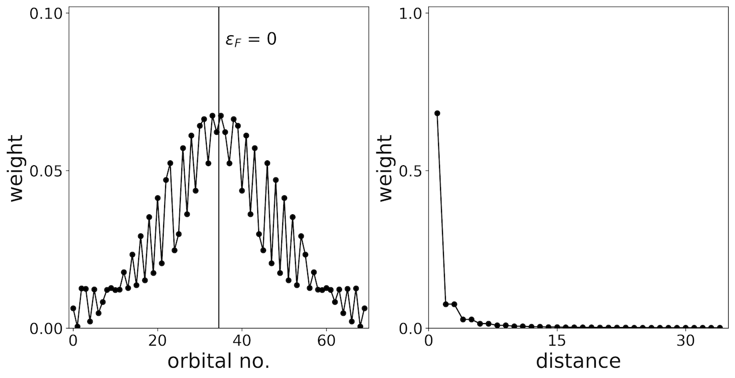
Figure 1.1: The characterization of bath subspace in DMET. The numerical experiment is performed on a half-filled 70-site tight-binding Hamiltonian with a 2-site fragment. Left panel: The squared norm of projections of canonical orbitals to the bath space, ordered by orbital energy. Right panel: The squared norm of projections of lattice sites to the bath space, ordered by the distance to the fragment (only half of the environmental sites are shown because of the inversion symmetry).

In the thesis work, we use DMET to study the cuprate high-temperature superconductivity (HTSC). HTSC has wide applications in the high-technology industries and scientific reseach, although these materials are still hard to make and require low temperatures to stay in the superconducting phase. The ultimate goal in the scientific studies of HTSC is to find systematic ways to increase its transition temperature. Despite the potential economic value, HTSC is also of much theoretical interest because of its mysterious pairing mechanism, as well as the rich phases other than superconductivity that emerge in the material [56, 57, 58, 59, 60].

Although the details are far from settled, we actually understand quite a lot qualitative understandings of cuprate HTSC. The key of HTSC in cuprates lies in the CuO₂ plane, which is shared by all the materials in this family. The essential physics of the CuO₂ plane is well approximated by the one- and three-band Hubbard model, and the even simpler $t$-$J$ model [61], in the sense that the most relevant phases in cuprates, such as antiferromagnetism, $d$-wave superconductivity, and various inhomogeneous charge, spin and pairing orders arise in theoretical analysis and/or numerical solutions of these models [62, 63, 64, 65, 66, 67, 68, 69, 53, 70]. The locations of these orders in the phase diagram are roughly known for both cuprates and these derived models. The most intriguing pseudogap phase, which may correspond to inhomogeneous orders in the ground state, has been studied both experimentally and theoretically, and have produced many theoretical hypotheses  [71, 72, 73, 74, 75, 76].

However, the problem in the studies of cuprate HTSC is that, although we understand what phases might appear in cuprates (and the Hubbard and $t$-$J$ models), and what mechanisms may be behind the phases, we do not know exactly what actually happens, because many of the candidate orders are packed in a small energy scale, and can be stabilized by small changes in the parameters. The low energy scale associated with the various competing orders makes it difficult to address the problem with pure theory or simple calculations; numerical studies without enough energy accuracy, although can produce various relevant orders in roughly correct regions, do not give a definitive answer either; while accurate, quasi-exact numerical studies usually can only be applied to finite clusters that are not large enough to support long-range orders. All it requires to solve the issue is concrete, numerically precise simulation to resolve all the competing states and mechanisms that appear in the material. Thus, DMET seems to have its unique advantage as it gives accurate estimates of ground state energy while supporting long-range order even with small fragment sizes (although to determine the energies and orders more accurately, larger fragment calculations are necessary to enable extrapolation).

Thus, the goal of my thesis work is to provide well-controlled numerical studies of HTSC that has enough energy resolution to distinguish the competing orders. We primarily work with the one-band Hubbard model because it seems a good balance between conciseness and validity, not to mention the historical importance of the model itself. Experimental realization of the Hubbard model ground state is also within reach in the next decades  [77, 78]. To reach this goal, we have (i) developed broken spin and particle-number symmetry DMET, which can bring the lattice mean-field solution to the correct phase; (ii) developed efficient impurity solvers that scales polynomial with the fragment size, that enables performing DMET on large fragments where rich physics can arise; (iii) determined the finite-size scaling that translates energies and observables from finite fragment calculations into quantities in the thermodynamic limit; and (iv) calibrated error estimators for energies and order parameters that allows us to draw concrete conclusions. As we will demonstrate, while the one-band Hubbard model is relevant to cuprates, it misses various important interactions in the real materials and has limitations regarding resolving the detailed low-energy physics of cuprates. Thus, we go beyond the one-band model to study the three-band Hubbard model and downfolded ab initio cuprate Hamiltonians, which take into account the missing interactions and can give material specific predictions.

The thesis is organized as follows. In Chapter 2, we discuss the theoretical formulation of DMET, including the basic idea, the broken-symmetry formulation, various impurity solvers and useful theories and techniques in implementation. Chapter 3 to Chapter 5 will focus on the one-band Hubbard model. Chapter 3 introduces a joint work to study the finite-size scaling of two forms of DMET algorithms. In Chapter 4, we present a calibrated ground-state phase diagram of the standard and frustrated 2D Hubbard model with a wide range of coupling strengths and dopings relevant to cuprates and the $d$-wave superconductivity. With DMET, the energy accuracy achieved is one to two orders of magnitude higher than previous studies. In Chapter 5, we introduce a joint work using various numerical methods to study the $1/8$-doping point of the 2D Hubbard model in depth, where we are able to definitively determine the ground state and various low-energy states. Chapter 6 presents a review of DMET studies of the three-band model and downfolded cuprate Hamiltonians. Finally, in Chapter 7, we lay out a finite-temperature DMET formulation which can be applied to study temperature-dependent properties of cuprates and other strongly correlated materials.

Chapter 2 Density Matrix Embedding Theory

2.1 Introduction

Density matrix embedding theory (DMET) [54, 55, 79] aims at accurately describing small fragments strongly coupled to an extended system. To achieve this goal, it focuses on correctly treating the quantum entanglement between fragments and their environment.

There are many conceptual similarities between DMET and dynamical mean-field theory (DMFT), a Green’s function based embedding method that treats strongly correlated fermion systems. Both of them obtain a mean-field-like solution for the entire system and build a set of bath states to represent the environmental degrees of freedom coupled to the fragment. They also both create an impurity model to compute the exact solution of the fragment, in the presence of the bath. Then that information is used to improve the mean-field solution of the entire system. The process is self-consistent in both methods.

Unlike DMFT, DMET uses wavefunctions as its primary variable. This choice gives DMET various advantages, such as better suited for ground state calculations, and that the number of bath states is finite, compared to the potentially infinite number of bath orbitals in DMFT, which allows DMET to have significantly smaller computational cost the DMFT. Thus, one can use DMET to treat systems or properties which were computationally intractable with DMFT.

This chapter will focus on the formulation of DMET for ground state calculations in lattice systems. We will introduce a finite-temperature formulation in Chapter 7. Other spectral, phononic and molecular extensions of DMET are out of the scope of this thesis work, but can be found in Refs. [80, 81, 82, 83, 84, 85]. Sec. 2.2 introduces the formulation of DMET for normal state calculations. Sec. 2.3 extends the formulation to superconducting states. Sec. 2.4 reviews impurity solvers developed or used as part of the thesis work. In Sec. 2.5, we will discuss issues in implementing DMET and strategies to deal with them.

2.2 Theoretical Framework

A large part of any embedding theory is determined by how the environment is represented in the embedding calculations. In DMET, this is done by the Schmidt decomposition of the approximate solution of the entire system. In Sections  2.2.1 and  2.2.2, we introduce the construction of the bath and the impurity model in detail. In Sec. 2.2.3, we introduce the correlation potential and how it is optimized. In Sec. 2.2.4, we discuss the necessity and ways to fit chemical potential in DMET. In Sec. 2.2.5, we introduce the computation of expectations values in DMET. Solving the impurity model is an important, but relatively separate part in DMET algorithms, so we introduce the impurity solvers separately in Sec. 2.4.

Throughout this section we will use a spinless notation to convey only the essential idea of DMET. Switching to the spinful representation is straightforward.

2.2.1 The Exact Embedding

The Fock space of electrons (the second-quantized representation of many-electron states) can be naturally partitioned into two subsystems. We simply divide the orbitals (single-particle states) into two sets (with the number of orbitals $n_{A}$ and $n_{B}$, respectively) and name them subsystem A and B. The Hilbert space of the entire system is thus the direct product of the subsystem Hilbert spaces, $\mathcal{H}=\mathcal{H}_{A}\otimes\mathcal{H}_{B}$. And the orthonormal basis of $\mathcal{H}$ is $\{|\psi_{i}^{A}\rangle|\psi_{j}^{B}\rangle\}$, where $\{|\psi_{i}^{A}\rangle\}$ and $\{|\psi_{j}^{B}\rangle\}$ are the orthonormal basis of $\mathcal{H}_{A}$ and $\mathcal{H}_{B}$, respectively.

Any state in $\mathcal{H}$ can then be written as

$$|\psi\rangle=\Psi_{ij}|\psi_{i}^{A}\rangle|\psi_{j}^{B}\rangle.$$ (2.1)

Note that we use the Einstein notation for implicit summation here. The coefficient $\Psi$ is a $2^{n_{A}}\times 2^{n_{B}}$ matrix.

We can perform the singular value decomposition (SVD) on this matrix, which gives $\Psi=U\Sigma V^{\dagger}$, where $U$ and $V$ are unitary matrices and $\Sigma$ is a diagonal matrix of dimension $2^{n_{A}}\times 2^{n_{B}}$. The number of non-zero elements in $\Sigma$ is $\min\{2^{n_{A}},2^{n_{B}}\}$. Without losing the generality, we assume $n_{A}\leq n_{B}$, and let the diagonal elements of $\Sigma$ be $\{\sigma_{k}\}(k=1,\cdots,2^{n_{A}})$, then

$$\Psi_{ij}=\sigma_{k}U_{ik}V_{jk}^{*}.$$ (2.2)

Let $|\alpha_{k}\rangle=U_{ik}|\psi_{i}^{A}\rangle$ and $|\beta_{k}\rangle=V_{jk}^{*}|\psi_{j}^{B}\rangle$, we have

$$|\psi\rangle=\sigma_{k}|\alpha_{k}\rangle|\beta_{k}\rangle.$$ (2.3)

$\{|\alpha_{k}\rangle\}$ and $\{|\beta_{k}\rangle\}$ are a special pair of biorthogonal basis in A and B, which (a) give a diagonal expansion of the wavefunction $|\psi\rangle$; and (b) the sizes of which equal to the size of the smaller subspace $\mathcal{H}_{A}$, which is $2^{n_{A}}$, even for the bigger subspace $\mathcal{H}_{B}$. (One can, of course, complete the basis of the larger subspace $\mathcal{H}_{B}$ with the complement of $|\beta_{k}\rangle$.)

This is called the Schmidt decomposition [86] of state $|\psi\rangle$. The coefficients $\sigma_{k}$ and basis $\alpha_{k}$, $\beta_{k}$ are Schmidt coefficients and Schmidt basis, respectively. The math of SVD guarantees that the Schmidt decomposition is unique (up to a phase), i.e., invariant of $\{|\psi_{i}^{A}\rangle\}$ and $\{|\psi_{i}^{B}\rangle\}$ chosen to perform the decomposition. It also implies that any biorthogonal basis pair satisfying Eq. 2.3 is the same Schmidt decomposition of $|\psi\rangle$, up to a phase.

The Schmidt decomposition naturally defines a set of bath for the fragment problem: if we let subsystem A be the fragment and the subsystem B be the rest, i.e., the environment, $\{|\alpha_{k}\rangle\}$ is a complete basis for the fragment, while $\{|\beta_{k}\rangle\}$ spans a small subspace in the environment with the following properties: (a) it has direct entanglement with the fragment; (b) its size equals to the size of the fragment, and thus independent of the size of the environment. We can thus define $\{|\beta_{k}\rangle\}$ as the bath, in which we solve the coupled fragment and bath problem by projecting the Hamiltonian to this subspace.

Thus, given the partition of the fragment and the environment, any wavefunction representation of the entire system defines a set of bath, with which one can embed the fragment in the environment quantum mechanically. In particular, in the limit where $|\psi\rangle$ is the exact ground-state wavefunction of the entire system, the embedding is exact. By exact embedding, we mean any observables in the fragment, obtained from the impurity model, equals to the same observables obtained by solving the entire lattice system exactly.

Suppose in Eq. 2.3, $|\psi\rangle=|\Psi\rangle$ is the ground state of the entire system, and the ground-state energy $E_{0}=\langle\Psi|\hat{H}|\Psi\rangle$. The bath Hilbert space is the space spanned by environmental Schmidt basis $\mathcal{H}_{\beta}=span\{|\beta_{k}\rangle\}$ while the fragment space is $\mathcal{H}_{\alpha}=span\{|\alpha_{k}\rangle\}$. We define the impurity model Hamiltonian in the space $\mathcal{H}_{\alpha}\otimes\mathcal{H}_{\beta}$ by projecting the entire system Hamiltonian $\hat{H}$ to the subspace

$$\hat{H}_{\text{emb}}=P\hat{H}P$$ (2.4)

where the projector

$$P=\sum_{k,l}|\alpha_{k}\rangle|\beta_{l}\rangle\langle\beta_{l}|\langle\alpha_{k}|.$$ (2.5)

Since $\langle\Psi|\hat{H}_{\text{emb}}|\Psi\rangle=\langle\Psi|P\hat{H}P|\Psi\rangle=\langle\Psi|\hat{H}|\Psi\rangle=E_{0}$, the ground state solution of the impurity model is exactly $|\Psi\rangle$, the same as the ground state of the entire system. It obvious matches all the observables with the exact ground state.

2.2.2 Embedding with Slater Determinants

The exact embedding is an ideal scenario but impossible to realize. After all, there is no point to do any embedding when we can obtain the exact solution for the entire system. Another subtle, but a much more serious issue is that the Schmidt decomposition of any general many-body wavefunction scales exponentially with the size of the entire lattice. It is thus desirable to find a class of approximate wavefunctions, which

• allows computationally tractable Schmidt decomposition; and

• can be systematically improved to approach the exact wavefunction.

It turns out that there is no perfect candidate that satisfies both properties. One can, however, loose the second condition to only require observables in the correlated fragment solution to be systematically improvable. In this case, Slater determinants can be used to approximate the lattice wavefunction.

A Slater determinant consists of a set of $N$ occupied orbitals (canonical orbitals) as linear combinations of $n$ local orbitals (i.e., atomic orbitals or lattice sites).

$$|\psi\rangle=c_{1}^{\dagger}\cdots c_{N}^{\dagger}|0\rangle.$$ (2.6)

The occupied orbitals $c_{p}^{\dagger}=C_{ip}a_{i}^{\dagger}$, where $a_{i}^{\dagger}$ creates an electron on site (orbital) $i$ and $C_{n\times N}$ is the orbital coefficient matrix. For simplicity, we assume both the cannonical orbitals and the local orbitals are orthonormal sets. The one-body density matrix is defined as

$$\rho_{ij}=\langle\psi|a_{i}^{\dagger}a_{j}|\psi\rangle=C_{ip}C_{jp}^{*}.$$ (2.7)

In matrix form, $\rho=CC^{\dagger}$. All higher-order density matrices and observables of the Slater determinants can be computed through the one-body density matrix. Also, the one-body density matrix is invariant under the rotations of occupied orbitals.

The Schmidt basis of Slater determinants can be constructed by the rotations of the occupied orbitals. Consider a bipartite of the system, where the first $n_{A}$ sites belong to subsystem A, and the other $n_{B}=n-n_{A}$ sites belong to subsystem B. We also assume $n_{A}<n_{B}$ and number of electrons $N>n_{A}$. In this setting, A is the fragment of interest, while B is the environment. There exists a unitary transformation of the coefficient matrix $C$, such that

$$\tilde{C}=CR=\begin{bmatrix}P&\mathbf{0}\\ Q&E\end{bmatrix}$$ (2.8)

where $R$ is a unitary matrix, $P$, $Q$ and $E$ are of dimensions $n_{A}\times n_{A}$, $n_{B}\times n_{A}$ and $n_{B}\times(n-n_{A})$, respectively. The upper right corner of the transformed coefficient matrix is zero, meaning all but $n_{A}$ occupied orbitals are restricted to subsystem B. As we have seen before, the transformation leaves the one-body density matrix, and thus the Slater determinant invariant, therefore

$$\begin{split}|\psi\rangle&=\prod_{k=1}^{n_{A}}\tilde{c}_{k}^{\dagger}\prod_{l=n_{A}+1}^{N}\tilde{c}_{l}^{\dagger}|0\rangle\\ &=\prod_{k=1}^{n_{A}}(p_{k}c_{A,k}^{\dagger}+q_{k}c_{B,k}^{\dagger})\prod_{l=n_{A}+1}^{N}c_{B,l}^{\dagger}|0\rangle\\ &=\sum_{i_{1},\cdots,i_{n_{A}}\in\{0,1\}}\prod_{k=1}^{n}p_{k}^{i_{k}}q_{k}^{1-i_{k}}|i_{1},\cdots,i_{n_{A}}\rangle_{A}\otimes|1-i_{1},\cdots,1-i_{n_{A}};\Psi_{c}\rangle_{B}\end{split}$$ (2.9)

where

$$c_{A,k}^{\dagger}=\frac{1}{p_{k}}\sum_{i=1}^{n_{A}}P_{ik}a_{i}^{\dagger},c_{B,k}^{\dagger}=\frac{1}{q_{k}}\sum_{j=1}^{n_{B}}Q_{j,k}a_{j+n_{A}}^{\dagger},c_{B,l}^{\dagger}=C_{l}^{\dagger}=\sum_{j=1}^{n_{B}}E_{j,l}a_{j+n_{A}}^{\dagger}$$ (2.10)

and $p_{k}=(\sum_{i=1}^{n_{A}}|p_{ik}|^{2})^{1/2}$, $q_{k}=(\sum_{i=1}^{n_{B}}|q_{ik}|^{2})^{1/2}$ are the normalization factors.

Note that the columns of $P,Q$ do not have to be orthogonal. But we will show later that there exists a set of $P,Q$ where the columns are orthogonal. (The columns of $Q$ are always orthogonal with columns of $E$.) If this is true, $c_{A,k}^{\dagger},c_{B_{k}}^{\dagger}$ are orthogonal fermions operators, and in particular $\{c_{A,k}^{\dagger}\}$ spans the Fock space of subsystem A. Under this condition, we used the following notation in Eq. 2.9

$$\begin{split}|i_{1},\cdots,i_{n_{A}}\rangle_{A}&=\prod_{k=1}^{n_{A}}(c_{A,k}^{\dagger})^{i_{k}}|0\rangle_{A}\\ |j_{1},\cdots,j_{n_{A}};\Psi_{c}\rangle_{B}&=\prod_{k=1}^{n_{A}}(c_{B,k}^{\dagger})^{j_{k}}|\Psi_{c}\rangle_{B}=\prod_{k=1}^{n_{A}}(c_{B,k}^{\dagger})^{j_{k}}\prod_{l=n_{A}+1}^{N}c_{B,l}^{\dagger}|0\rangle_{B}.\end{split}$$ (2.11)

Eq. 2.11 defines a pair of biorthogonal basis for subsystem A and B, and, according to the uniqueness of Schmidt decomposition, Eq. 2.9 is actually the Schmidt decomposition of the Slater determinant. The impurity model is thus equivalent to solving the complete active space (CAS) problem with active orbitals $\{c_{A_{k}}^{\dagger},c_{B_{k}}^{\dagger}\}(k\in[1,n_{A}])$ and core orbitals $\{c_{B_{l}}\}(l\in[n_{A}+1,N])$. Since the rotation within the active space does not affect the solution, we can simply use the site basis $\{a_{i}^{\dagger}\}(i\in[1,n_{A}])$ instead of $\{c_{A_{k}}^{\dagger}\}$. Thus, only the bath and core orbitals $\{c_{B_{k}}^{\dagger}\}$ need to be specified for the impurity model. (Note the bath orbitals are related to but different from the bath states $\{|\beta_{k}\rangle\}$ from Sec. 2.2.1 which are many-body states.)

There are a few different but equivalent approaches to obtain the bath orbitals using the one-body density matrix. Use $\tilde{C}=CR$ to compute the one-body density matrix, we have

$$\rho=\tilde{C}\tilde{C}^{\dagger}=\begin{bmatrix}PP^{\dagger}&PQ^{\dagger}\\ QP^{\dagger}&QQ^{\dagger}+EE^{\dagger}\end{bmatrix}=\begin{bmatrix}\rho_{A}&\rho_{AB}\\ \rho_{AB}^{\dagger}&\rho_{B}\end{bmatrix}.$$ (2.12)

Let $\rho_{A}=U\Gamma U^{\dagger}$ be the eigendecomposition, then we have $P=U\Gamma^{1/2}$, and $Q=(P^{-1}\rho_{AB})^{\dagger}$. The bath orbitals are thus defined by normalizing each column of $Q$. Note that here the columns of $P$ are orthogonal, because $U$ is unitary and $\Gamma^{1/2}$ is diagonal. Since $PP^{\dagger}+QQ^{\dagger}=I$, it follows that the columns of $Q$ are also orthogonal. One can perform a simple transformation, for instance, $P^{\prime}=PT$ and $Q^{\prime}=Q(T^{-1})^{\dagger}$ where $T$ is any non-singular square matrix, to make columns of $P^{\prime}$ and $Q^{\prime}$ non-orthogonal. This verifies our claim that the representation in Eq. 2.8 is not unique, and there exist solutions where columns of $P$ and $Q$ are orthogonal.

An equivalent way to obtain bath orbitals is to diagonalize the environmental part of the density matrix $\rho_{B}$. The eigenstates with eigenvalues between 0 and 1 are the bath orbitals, while those with eigenvalue 1 are core orbitals. One can as well perform SVD on $\rho_{AB}=U\Sigma V^{\dagger}$, where the matrix $V$ gives the orthonormalized coefficients of bath orbitals.

In summary, given a Slater determinant, we can formulate the embedding calculation by obtaining the bath and core orbitals of the environment, and the impurity model becomes a CASCI problem.

2.2.3 Correlation Potential

In Sec. 2.2.2, we present in detail how to perform an embedding calculation given a Slater determinant wavefunction of the lattice. We now discuss the parameterization and optimization of the determinant.

In DMET, the determinant is parameterized as the ground state of a non-interacting Hamiltonian

$$H_{\text{mf}}=h+u$$ (2.13)

where the core Hamiltonian $h$ is either the one-body part of the full Hamiltonian $H_{1}$, or the Fock matrix $F$, depending on the nature of the problem. For instance, in lattice problems where the interactions are usually local, the bare one-body Hamiltonian $H_{1}$ is preferred; while in molecular calculations, it is better to use the Fock matrix $F$. The additional one-body term $u$, usually called the correlation potential, mimics the effective two-body interaction, is to be determined.

Compared to using the orbital coefficients $C$ as primary variable, an auxiliary potential $u$ is favored in various ways: the constraints on the $u$ (Hermitian) is much simpler than the constraints on $C$ (unitary), and there is strong physical interpretations for $u$ as the effective potential due to electron correlation.

To approximate the behavior of local correlation, we restrict the correlation potential to be local to each fragment. In lattice systems, it means $u$ is block-diagonal on the supercells chosen as fragments, and each diagonal block is identical because of the translational invariance.

$$u=\begin{bmatrix}u_{C}&&&\\ &\ddots&&\\ &&u_{C}&\\ &&&u_{C}\end{bmatrix}.$$ (2.14)

Given the correlation potential $u$, one obtains the lattice Slater determinant $|\psi\rangle$ and the correlated wavefunction $|\psi_{\text{emb}}\rangle=|\Psi\rangle\otimes|\Psi_{c}\rangle$. In the notation, $|\Psi\rangle$ is the correlated wavefunction of the impurity model (fragment + bath), while $|\Psi_{c}\rangle$ is the core environmental wavefunction defined in Sec. 2.2.2. It becomes apparent that using Slater determinant to construct the impurity model does not change any expectation values in the core space. Therefore, one only expects the observables in the fragment to improve upon the mean-field results. Because one has no access to the exact values of these observables, to evaluate the quality of the embedding calculation, and thus $u$, we use the similarity between $|\psi\rangle$ and $|\psi_{\text{emb}}\rangle$.

There are many metrics to choose from, but with DMET, the most common choice is the one-body density matrix. The cost function is thus

$$f(u)=||\rho_{\Psi}(u)-\rho_{\psi}(u)||^{2}$$ (2.15)

where $\rho_{\Psi,ij}$ is the one-body density matrix of the correlated wavefunction and $\rho_{\psi}$ is the that of the Slater determinant, both in the basis of the impurity model. Minimizing the cost thus minimizes the difference between the mean-filed level and correlated solutions of the impurity model at one-particle level. There are various implications of this cost function:

• Both the fragment and bath parts of the density matrix were used, indicating that we try to maintain a balance between the accuracy of the fragment itself and its coupling to the environment.

• Since the mean-field density matrix $\rho_{\psi}$ is idempotent (even when projected to the impurity model), generally the cost function cannot be reduced to zero.

Other cost functions, such as the density matrix difference on the fragment, or even simpler, the difference in occupation numbers of the fragment orbitals , were proposed [87]. Empirically, we find the full density matrix formulation works best for lattice models, probably because of the balance it achieves between the fragment itself and the coupling to the environment.

Eq. 2.15 defines an unconstrained optimization problem, which one can solve with standard minimization procedure. However, the gradient of the cost function is

$$f^{\prime}(u)=\sum_{ij}(\rho_{\Psi,ij}(u)-\rho_{\psi,ij}(u))(\frac{d\rho_{\Psi,ij}}{du}-\frac{d\rho_{\psi,ij}}{du})$$ (2.16)

where the response of $\rho_{\Psi}$ with respect to changes in $u$ cannot be computed analytically and the numerical gradient involves solving the impurity model multiple times. Therefore, we use a self-consistent procedure to perform the minimization

1. Compute $\rho_{\Psi}^{*}=\rho_{\Psi}(u)$.

2. $\min_{u}f(u)=||\rho_{\Psi}^{*}-\rho_{\psi}(u)||^{2}$ with $\rho_{\Psi}^{*}$ fixed; If $||\Delta u||>\varepsilon_{u}$, go back to step 1.

Here $\varepsilon_{u}$ is the convergence threshold for the correlation potential $u$.

One last issue related to the correlation potential is the choice of impurity model Hamiltonian. In exact embedding, we simply project the entire lattice Hamiltonian to the impurity model (Eq. 2.4). We can continue using this approach when embedding with Slater determinants; because there are electron interactions between bath orbitals, this approach is often referred as the interacting bath. Alternatively, one can use the correlation potential to replace the electron interactions on bath orbitals, and include the interactions only between the fragment orbitals, called the non-interacting bath

$$\hat{H}_{\text{emb}}^{\text{NI}}=P[H_{1}+u+P_{F}(H_{2}-u)P_{F}]P$$ (2.17)

where $H_{2}$ is the two-body part of the original Hamiltonian, and $P_{F}$ is the projection to the fragment. The non-interacting bath has an origin analogous to those used in the DMFT impurity model, which are restricted to be non-interacting and varied to match the hybridization function.

It is often preferable to use the non-interacting bath formulation in lattice DMET calculations, although the interacting bath seems more elegant. There are various theoretical arguments for that. One argument is that embeddings from Slater determinants may not have enough flexibility to obtain a good enough approximation for the ground state Schmidt basis, while the non-interacting approach, by directly encoding $u$ in the impurity Hamiltonian, can access a larger space to approximate the ground state properties of the fragment efficiently. Another more physical argument is that, since the bath orbitals in lattice systems often extend many unit cells, the screening plays a role and it is well-known that direct downfolding of the electron interactions works poorly in this context. The use of $u$ to replace these long-range interactions in the non-interacting bath, to some extent, renormalizes the electron interaction and could improve the results. Computationally, the non-interacting bath is also favored as it avoids the task of sometimes formidable integral transformation which scales $O(n^{5})$ with the size of the entire lattice.

The detailed equations and algorithms for this section are presented in Appendix B.3.

2.2.4 Chemical Potential Optimization

A problem in the embedding calculations is how to control the number of electrons in the fragment. Following the embedding formulation in Sec. 2.2.2 and  2.2.3, there is no guarantee what number of electrons in the fragment we get from impurity model calculations. This does not only affect the values of the observables, but is itself problematic in a lattice problem, where the number of electrons per fragment is usually well defined. It is thus desirable to have the number of electrons exactly match what we expect for the lattice model.

To do so, we introduce the chemical potential term $\mu$. We recognize that there is a gauge freedom between $\mu$ and the diagonal terms of correlation potential $u$ in the mean field, i.e.,

$$\mu^{\prime}=\mu+\phi,\thinspace u^{\prime}=u+\phi\sum_{i}a_{i}^{\dagger}a_{i}.$$ (2.18)

This gauge freedom is lost in the impurity model calculation with non-interacting bath, as one can see in Eq. 2.17 that the correlation potential is only added to the bath orbitals. Therefore, one can vary $\mu$ and the diagonal of $u$ together following Eq. 2.18 so that the mean-field solution (thus the bath orbitals) does not change, while the relative energy levels of the fragment and the bath orbitals are shifted. Thus, we can perform chemical potential optimization while solving the impurity model. The chemical potential obtained in this procedure is usually a good approximation of the chemical potential in the physical sense. The details of a self-adaptive chemical potential fitting algorithm, and how it is built into the DMET iterations are explained in Appendix B.4.

2.2.5 Expectation Values

In general, there are two types of expectation values of interest in DMET. Local observables, such as occupations and local order parameters can be directly computed using the correlated wavefunction $|\Psi\rangle$. These expectation values should be computed only if they are fully within the fragment. Reciprocal space observables, such as band structure and spin structure factors, cannot be formally defined for DMET correlated wavefunction $|\Psi\rangle\otimes|\Psi_{c}\rangle$ because of the lack of translational invariance. One could, however, obtain rough estimates from the associated lattice Slater determinants. Other nonlocal observables, such as long-range correlation functions, can be computed by taking expectation values of the locally correlated entire system wavefunction $|\Psi\rangle\otimes|\Psi_{c}\rangle$. However, these observables will have a smooth transition from the full many-body results to the mean-field values, and are seldom of practical use.

Another important expectation value is the energy per supercell (fragment). Note the DMET energy is different from the impurity model energy $E_{\text{emb}}=\langle\Psi|\hat{H}^{\text{(NI)}}_{\text{emb}}|\Psi\rangle$. We consider the bipartite decomposition of the lattice Hamiltonian

$$\hat{H}=H_{\text{frag}}+H_{\text{env}}+H_{\text{frag-env}}.$$ (2.19)

Obviously, the fragment part $H_{\text{frag}}$ should be included and $H_{\text{env}}$ should not. The coupling term $H_{\text{frag-env}}$ is split between the fragment and environment, by taking a partial trace of the second-quantized terms, i.e.

$$e_{\text{frag}}=\sum_{i\in\text{fragment},j}h_{ij}\rho_{ij}+\frac{1}{2}\sum_{i\in\text{fragment},jkl}(ik||jl)\Gamma_{ik,jl}$$ (2.20)

where $\rho_{ij}$ and $\Gamma_{ik,jl}=\langle\Psi|\langle\Psi_{c}|a_{i}^{\dagger}a_{j}^{\dagger}a_{l}a_{k}|\Psi\rangle|\Psi_{c}\rangle$ are one- and two-body density matrices of the correlated wavefunction $|\Psi\rangle\otimes|\Psi_{c}\rangle$. This is equivalent to a full trace, with scaling factors equal to the fraction of the indices in the fragment. (For example, for term $(ik||jl)\Gamma_{ik,jl}$ where indices $i,k,l$ are in the fragment, the scaling factor is $3/4$.) This is an intuitive way to understand the decomposition of the coupling energy.

2.3 The Broken Particle-Number Symmetry Formalism

In this section, we extend the generic DMET formulation to broken particle-number symmetry problem. They correspond to systems with superconductivity, where the pairing order parameters $\langle a_{i\alpha}^{\dagger}a_{j\beta}^{\dagger}\rangle$ are non-zero (The $\alpha$ and $\beta$ are spin labels. We consider singlet pairing only.)

Historically, superconducting wavefunctions with broken particle-number symmetry were first obtained in the mean-field solution of fermion systems with effective attractive interactions, induced by electron-phonon coupling  [88, 89]. The size of the broken particle-number symmetry, measured by the magnitudes of pairing terms, describes the existence and robustness of the superconductivity. In pure electronic systems, such as the high-temperature superconductors, there are no attractive terms between electrons, and mean-field solutions never spontaneously break the particle number symmetry, although the exact solution in the thermodynamic limit has long-range pairing correlations. In DMET, however, we can enable pairing in the correlation potential, which is determined self-consistently, and it turns out the superconducting solutions can be stabilized spontaneously.

In Sec. 2.3.1 and  2.3.2, we introduce the mean-field and embedding aspects of DMET in the presence of pairing. In our derivation, the spin-unrestricted formulation is used. In Sec. 2.3.3, we discuss why this formulation can give correct results of superconductivity.

2.3.1 The BCS Wavefunction and BdG Equation

The spin-unrestricted Bogoliubov transformation is defined as

$$\begin{split}c_{p\alpha}^{\dagger}&=u^{\alpha}_{ip}a_{i\alpha}^{\dagger}+v^{\beta}_{iq}a_{i\beta}\\ c_{p\beta}^{\dagger}&=u^{\beta}_{ip}a_{i\beta}^{\dagger}+v^{\alpha}_{iq}a_{i\alpha}\end{split}$$ (2.21)

where $c_{p\sigma}^{\dagger}$ creates a quasiparticle of spin $\sigma$, $a_{i\sigma}^{\dagger}$ creates an electron of spin $\sigma$ in orbital $i$. For simplicity, we assume the coefficients are all real numbers. The quasiparticles defined here have good $S_{z}$ quantum numbers, but the particle number symmetry is broken. This is the so-called singlet pairing that preserves $S_{z}$ symmetry, and is usually the case in both conventional and high-temperature superconductors.

The transformation can also be written in matrix form

$$\begin{bmatrix}c_{\alpha}^{\dagger}&c_{\beta}\end{bmatrix}=\begin{bmatrix}a_{\alpha}^{\dagger}&a_{\beta}\end{bmatrix}\begin{bmatrix}U_{\alpha}&V_{\alpha}\\ V_{\beta}&U_{\beta}\end{bmatrix}=\begin{bmatrix}a_{\alpha}^{\dagger}&a_{\beta}\end{bmatrix}S.$$ (2.22)

A complete set of Bogoliubov transformation has $n$ orthonormal quasiparticles for each spin. In this case, the matrix $S$ is unitary (one can verify it by checking the anticommutators), therefore

$$U_{\sigma}U_{\sigma}^{\dagger}+V_{\sigma}V_{\sigma}^{\dagger}=I,\thinspace V_{\sigma}U_{\bar{\sigma}}^{\dagger}+U_{\sigma}V_{\bar{\sigma}}^{\dagger}=0$$ (2.23)

and the inverse Bogoliubov transformation

$$\begin{bmatrix}a_{\alpha}^{\dagger}&a_{\beta}\end{bmatrix}=\begin{bmatrix}c_{\alpha}^{\dagger}&c_{\beta}\end{bmatrix}S^{\dagger}=\begin{bmatrix}c_{\alpha}^{\dagger}&c_{\beta}\end{bmatrix}\begin{bmatrix}U_{\alpha}^{\dagger}&V_{\beta}^{\dagger}\\ V_{\alpha}^{\dagger}&U_{\beta}^{\dagger}\end{bmatrix}.$$ (2.24)

A BCS wavefunction $|\psi\rangle$ are defined as the vacuum of a complete set of Bogiliubov quasiparticles, i.e.,

$$c_{p\sigma}|\psi\rangle=0.$$ (2.25)

Like the Slater determinants, the observables of BCS wavefunctions are also determined entirely by its one-body density matrices. Besides the standard one-body density matrices, BCS wavefunctions have non-zero pairing density matrices $\kappa^{\alpha\beta}_{ij}=\langle\psi|a_{i\alpha}a_{j\beta}|\psi\rangle$. The density matrices of BCS wavefunctions can be evaluated using Eq. 2.24 and  2.25, thus

$$\begin{split}G=&\begin{bmatrix}\rho_{\alpha}&\kappa_{\beta\alpha}^{\dagger}\\ \kappa_{\beta\alpha}&I-\rho_{\beta}^{T}\end{bmatrix}=\langle\psi|\begin{bmatrix}a_{\alpha}^{\dagger}\\ a_{\beta}\end{bmatrix}\begin{bmatrix}a_{\alpha}&a_{\beta}^{\dagger}\end{bmatrix}|\psi\rangle\\ =&\langle\psi|S\begin{bmatrix}c_{\alpha}^{\dagger}\\ c_{\beta}\end{bmatrix}\begin{bmatrix}c_{\alpha}&c_{\beta}^{\dagger}\end{bmatrix}S^{\dagger}|\psi\rangle=S\begin{bmatrix}0&0\\ 0&1\end{bmatrix}S^{\dagger}=\begin{bmatrix}V_{\alpha}V_{\alpha}^{\dagger}&V_{\alpha}U_{\beta}^{\dagger}\\ U_{\beta}V_{\alpha}^{\dagger}&U_{\beta}U_{\beta}^{\dagger}\end{bmatrix}\end{split}$$ (2.26)

i.e.,

$$\rho_{\sigma}=V_{\sigma}V_{\sigma}^{\dagger},\thinspace\kappa_{\beta\alpha}=-\kappa_{\alpha\beta}^{T}=U_{\beta}V_{\alpha}^{\dagger}.$$ (2.27)

$G$ is the generalized one-body density matrix of $|\psi\rangle$, as it contains the information of all the channels of the one-body density matrices.

The BCS wavefunctions are the ground state solutions of non-interacting Hamiltonians with pairing terms

$$\hat{H}=h_{ij\sigma}a_{i\sigma}^{\dagger}a_{j\sigma}+\Delta_{ij}a_{i\alpha}^{\dagger}a_{j\beta}^{\dagger}+h.c..$$ (2.28)

It is also the mean-field solution of an interacting Hamiltonian, with the assumption that $\langle a_{i\alpha}a_{j\beta}\rangle\neq 0$. In this case, the two-body terms are approximated as

$$\langle a_{i\mu}^{\dagger}a_{j\nu}^{\dagger}a_{l\nu}a_{k\mu}\rangle\approx\langle a_{i\mu}^{\dagger}a_{k\mu}\rangle\langle a_{j\nu}^{\dagger}a_{l\nu}\rangle-\delta_{\mu\nu}\langle a_{i\mu}^{\dagger}a_{l\mu}\rangle\langle a_{j\mu}^{\dagger}a_{k\mu}\rangle+\delta_{\mu\bar{\nu}}\langle a_{i\mu}^{\dagger}a_{j\nu}^{\dagger}\rangle\langle a_{l\nu}a_{k\mu}\rangle$$ (2.29)

where the first two terms are Coulomb and exchange terms in Hartree-Fock theory, while the last term comes from pairing. This formulation is thus called Hartree-Fock-Bogoliubov (HFB) theory. By forming the Fock matrix, HFB essentially solves for the ground state of an effective Hamiltonian similar to that in Eq. 2.28 as well. The pairing density matrix becomes non-zero for certain values of the two-body interactions.

In both cases, the problem reduces to finding the quasiparticles by solving the Bogoliubov-de Gennes (BdG) equation [90], in analogous to the Hartree-Fock-Roothaan equation in Hartree-Fock theory. Given the chemical potential $\mu$, the BdG equation is [91]

$$\begin{bmatrix}h_{\alpha}-\mu I&\Delta\\ \Delta^{\dagger}&-h_{\beta}+\mu I\end{bmatrix}\begin{bmatrix}U_{\alpha}&V_{\alpha}\\ V_{\beta}&U_{\beta}\end{bmatrix}=\begin{bmatrix}U_{\alpha}&V_{\alpha}\\ V_{\beta}&U_{\beta}\end{bmatrix}\begin{bmatrix}\varepsilon_{\alpha}&\\ &-\varepsilon_{\beta}\end{bmatrix}$$ (2.30)

where $\varepsilon_{\alpha}$ and $\varepsilon_{\beta}$ are all positive. The number of $\{\varepsilon_{\alpha}\}$ equals to the number of $\{\varepsilon_{\beta}\}$ for a $S_{z}=0$ system. One can also see from here why the ground state of Eq. 2.28 is the quasiparticle vacuum, since the Hamiltonian is transformed to

$$\hat{H}=E_{0}+\sum_{p\sigma}\varepsilon_{p\sigma}c_{p\sigma}^{\dagger}c_{p\sigma}$$ (2.31)

where $E_{0}=\langle\psi|\hat{H}|\psi\rangle$ is the ground state energy.

To apply the BCS formulation to DMET, we allow the correlation potential to include pairing terms, i.e.

$$u_{C}=\sum_{ij\sigma}h_{ij\sigma}a_{i\sigma}^{\dagger}a_{j\sigma}+\sum_{ij}\Delta_{ij}a_{i\alpha}^{\dagger}a_{j\beta}^{\dagger}+h.c.$$ (2.32)

where $i,j$ go over all the sites in a fragment. The mean-field solution $|\psi\rangle$ now becomes a BCS wavefunction. To obtain the correct mean-field solution, one needs to adjust the chemical potential $\mu$ so that $|\psi\rangle$ gives the pre-defined number of electrons.

2.3.2 Embedding the Quasiparticles

In this section, we take the mean-field BCS wavefunction and discuss the formation of the bath orbitals. At first look, the BCS wavefunction, defined as the quasiparticle vacuum, is not a product state and thus not possible to perform the Schmidt decomposition analogous to Slater determinants. As shown in Ref. [92], the Schmidt decomposition of a BCS wavefunction is equivalent to finding an embedded quasiparticle active space. Here, we introduce a new approach that converts the BCS wavefunction to a product state [93], which results in similar mathematical operations to the case of Slater determinants.

We start by defining a simple vacuum (background) $|\mathrm{vac}\rangle$ as a ferromagnetic state where all the $n$ lattice sites are occupied by spin-down ($\beta$) electrons, and let the quasiparticles

$$d_{p\alpha}^{\dagger}=c_{p\beta}.$$ (2.33)

We have $d_{p\alpha}|\mathrm{vac}\rangle=0$ and $c_{p\alpha}|\mathrm{vac}\rangle=0$ since $d_{p\alpha}$ and $c_{p\alpha}$ bring down $S_{z}$ by $1/2$, but $|{\mathrm{vac}}\rangle$ is already the lowest eigenstate of $S_{z}$.

We can thus write the BCS wavefunction as

$$|\psi\rangle=\prod_{p}d_{p\alpha}^{\dagger}|\mathrm{vac}\rangle$$ (2.34)

up to a phase, because the state on the right-hand side is the quasiparticle vacuum of $\{c_{p\sigma}\}$:

$$\begin{split}c_{p\alpha}(\prod_{q}d_{q\alpha}^{\dagger}|\mathrm{vac}\rangle)&=(-)^{n}\prod_{q}c_{q\beta}c_{p\alpha}|\mathrm{vac}\rangle=0\\ c_{p\beta}(\prod_{q}d_{q\alpha}^{\dagger}|\mathrm{vac}\rangle)&=c_{p\beta}\prod_{q}c_{q\beta}|\mathrm{vac}\rangle=0.\end{split}$$ (2.35)

Since Eq. 2.34 rewrites the BCS state into a product state (the vacuum $|\mathrm{vac}\rangle$ is also a product state), we view it as a Slater determinant with the occupied orbitals $\{d_{p\alpha}^{\dagger}\}$, and its one-body density matrix can be obtained using the orbital coefficients of $\{d_{p\alpha}^{\dagger}\}$

$$d_{\alpha}^{\dagger}=c_{\beta}=\begin{bmatrix}a_{\alpha}^{\dagger}&a_{\beta}\end{bmatrix}\begin{bmatrix}V_{\alpha}\\ U_{\beta}\end{bmatrix}.$$ (2.36)

It thus turns out the density matrix of $\{d_{p\alpha}^{\dagger}\}$ is acutally the generalized density matrix (Eq. 2.26) of $|\psi\rangle$. The Schmidt decomposition of $|\psi\rangle$ is then

$$|\psi\rangle=\prod_{k=1}^{2n_{A}}(p_{k}d_{A,k}^{\dagger}+q_{k}d_{B,k}^{\dagger})|\mathrm{vac}\rangle_{A}\otimes\prod_{l=2n_{A}+1}^{n}d_{B,l}^{\dagger}|\mathrm{vac}\rangle_{B}$$ (2.37)

where the notations are similar to those in Eq. 2.9. The $|\mathrm{vac}\rangle_{A}$ and $|\mathrm{vac}\rangle_{B}$ states are the ferromagnetic states of the fragment and the environment, respectively. The bath and core orbitals $d_{B}^{\dagger}$ can be obtained by diagonalizing the environmental part of the generalized density matrix $G_{B}$, similar to normal state DMET.

Note that the fragment and bath orbitals obtained in this procedure are all of spin $\alpha$, and the core state has spin $-n_{A}$. (the factor $1/2$ from electron spin is taken into account.) The impurity model is thus a spinless fermionic system of $4n_{A}$ sites in which $2n_{A}$ are occupied. Alternatively, we can perform a partial particle-hole transformation on half of the $4n_{A}$ modes, and make the core $S_{z}=0$. The impurity model then becomes a fermion problem of $2n_{A}$ (spatial) orbitals without particle-number symmetry, while $S_{z}=0$. The latter is used in the thesis work, because the pairing is usually a small effect in the problems of interest, thus the partial particle-hole transformation results in a better physical picture, where all the quasiparticles become electron-like (i.e. $||v||>||u||$), and fits better into available impurity solvers.

After the partial particle-hole transformation, the impurity model consists of $n_{A}$ fragment orbitals $\{a_{i\sigma}^{\dagger}\}$ and $n_{A}$ bath orbitals for each spin

$$d_{B,\alpha}^{\dagger}=a_{\alpha}^{\dagger}V_{B,\alpha}+a_{\beta}U_{B,\beta},\thinspace d_{B,\beta}^{\dagger}=a_{\beta}^{\dagger}V_{B,\beta}+a_{\alpha}U_{B,\alpha}.$$ (2.38)

And the core wavefunction becomes

$$|\Psi_{c}\rangle=\prod_{k=1}^{n_{A}}d_{B,k\beta}\prod_{l=2n_{A}+1}^{n}d_{B,l}^{\dagger}|\mathrm{vac}\rangle_{B}.$$ (2.39)

We discuss how to project the lattice Hamiltonian to the embedding basis in Appendix A.1.

2.3.3 Broken Symmetry DMET

We have discussed how to construct the impurity model with broken particle-number symmetry. The correlation potential and chemical potential optimizations are similar to the case of the normal state, although the math becomes more complicated (detailed in the Appendix). Here, we discuss the physical side of broken symmetry DMET calculations, i.e.,

• When and how does DMET give a broken symmetry solution?

• What controls the quality of order parameters obtained in DMET?

• How do the DMET orders connect to the exact solutions in the thermodynamic limit?

We use the example of pairing order to address these questions. By including pairing terms in the correlation potential, we obtain a BCS mean-field solution. That gives an impurity model Hamiltonian with non-zero pairing terms in the environmental degrees of freedom. This can be viewed as a pinning field similar to those used in finite lattice calculations, although more complicated and structured. The pinning field thus induces non-zero pairing orders in the fragment, the magnitude of which depends on the susceptibility of the fragment.

In the correlation potential fitting stage, we try to match the lattice wavefunctions to the correlated solutions, thus forcing the mean-field order parameters to increase or decrease adaptively, and changing the magnitudes of the pinning field and the order parameters in the correlated calculations. At convergence, the order parameters obtained in the impurity model calculations thus become a good approximation of the actual long-range order. The order parameters become exact in the limit of infinitely large fragments.

If the true ground state of the entire lattice has a long-range order, the susceptibility is infinite and the symmetry is spontaneously broken. In this case, DMET will also give a broken symmetry solution, which does not disappear as the size of the fragment grows. If, however, the order is short-ranged, the order parameters ultimately decay to zero as the distance to the fragment boundaries grows. In practice, these order parameters are often zero even with minimal fragment sizes thanks to DMET self-consistency.

In the case where long-range order does exist, one can obtain the exact order parameter by growing the fragment size to infinity. Alternatively, we can compute the order parameters with several fragment sizes and extrapolate to the thermodynamic limit. (It usually extrapolates to zero if the order is short-ranged.) Thus, the accuracy of these order parameters are determined by the largest sizes we can achieve in DMET calculations, as well as the function forms used for the extrapolation.

In summary, DMET coupled with finite size extrapolation is possible to exract order parameters in the thermodynamic limit. In Sec. 2.5.3 and Chapter 3, we will introduce the theory and empirical studies of DMET fragment size extrapolation.

2.4 Impurity Solvers

Impurity solvers are used to solve the quantum many-body problem the impurity models, either exactly or approximately. An advantage of DMET is that one can choose from a wide range of solvers already developed in the quantum chemistry or computational condensed matter communities, depending on the problems at hand. In this section, we introduce the common impurity solvers, both for normal state calculations and BCS calculations. We will focus on the principles and the appropriate contexts of these solvers.

2.4.1 Exact Diagonalization

The most direct way is to diagonalize the many-body Hamiltonian and obtain the full Fock space representation of the ground-state wavefunction. We write the wavefunction as an expansion of the occupation strings (subject to symmetries)

$$|\Psi\rangle=\sum_{n_{1},n_{2},\cdots,n_{K}}C_{n_{1},n_{2},\cdots,n_{K}}|n_{1},n_{2},\cdots,n_{K}\rangle$$ (2.40)

where $n_{k}\in\{|0\rangle,|\alpha\rangle,|\beta\rangle,|\alpha\beta\rangle\}$ is the occupation of orbital $k$. In exact diagonalization (ED), We minimize the total energy and find the optimal coefficients $C_{n_{1},n_{2},\cdots,n_{K}}$. The method is also called full configurational interaction (FCI) because of the Fock space expansion. The cost of ED scales exponentially with the system size, as we can see, the number of parameters in the giant tensor $C_{n_{1},n_{2},\cdots,n_{K}}$ scales $O(4^{K})$. In addition, naive eigendecomposition requires writing down the Hamiltonian matrix in this basis, and then perform the diagonalization routine, which takes $O(N^{2})$ space and $O(N^{3})$ time. The computational cost soon becomes formidable with about merely 8 to 10 orbitals.

We can save some memory and computational cost using the Lanczos or Davidson algorithms [94, 95] to compute only the lowest one or several eigenstates without explicitly writing down the Hamiltonian matrix. This is often referred as the direct CI [96, 97]. The Davidson algorithm is described in Appendix  B.5 in detail. The most time-consuming step in direct CI is to compute $\hat{H}|\Psi\rangle$, which is achieved by taking the each individual term in $\hat{H}$ and acting on each occupation string in the expansion of $|\Psi\rangle$. This, in fact, uses the sparsity of the Hamiltonian matrix and results in roughly $O(K^{4}4^{K})$ time complexity (terms in $\hat{H}$ $\times$ basis in $|\Psi\rangle$).

Due to the exponential complexity, even with Davidson algorithm, ED (or FCI) is able to treat only up to $\sim 20$ orbitals with current computational power. It is of limited uses as a DMET impurity solver, but can serve as the benchmark for other approximate impurity solvers.

2.4.2 Density Matrix Renormalization Group

The density matrix renormalization group (DMRG) [37, 38, 40] approximates the exact wavefunction coefficients Eq. 2.40 as the a tensor product

$$C_{n_{1},n_{2},\dots,n_{K}}=\sum_{i_{1},\dots,i_{K}}A_{i_{1}}^{n_{1}}A_{i_{1},i_{2}}^{n_{2}}\dots A_{i_{K-1}}^{n_{K}}.$$ (2.41)

The representation is called the matrix product states (MPS) because each $A^{n_{k}}$ is a matrix. The uncontracted indices $\{n_{k}\}$ are called the physical indices, while $\{i_{k}\}$ are called the auxiliary indices.

Eq. 2.41 is exact if we allow the dimensions of auxiliary indices $i_{k}$ to reach $4^{[K/2]}$, though in this case, the number of parameters scales exponentially. In practice, the dimension is restricted to have the maximum bond dimension $M$. The expression thus becomes a variational ansatz, whose accuracy is a monotonically increasing function of $M$.

DMRG is an efficient algorithm to optimize the MPS using the sweep algorithm, i.e., the tenors $\{A^{n_{k}}\}$ are updated one at a time, from left to right (forward) and then from right to left (backward), until the energy is converged. In each step during the sweep, one projects the Hamiltonian to a renormalized subspace around orbital $k$ and solve for the ground state. The subspace wavefunction is then compressed to keep the bond dimension $M$ unchanged during the calculation.

Specifically, when optimizing tensor $A^{n_{k}}$ in the forward sweep, the Hamiltonian is projected onto the basis

$$|\psi_{i_{k-1},n_{k},n_{k+1},i_{k+1}}\rangle=|L_{i_{k-1}}\rangle\otimes|n_{k}n_{k+1}\rangle\otimes|R_{i_{k+1}}\rangle$$ (2.42)

where

$$\begin{split}|L_{i_{k-1}}\rangle=&\sum_{i_{1},\dots,i_{k-2}}A_{i_{1}}^{n_{1}}\dots A_{i_{k-2},i_{k-1}}^{n_{k-1}}|n_{1},\dots,n_{k-1}\rangle\\ |R_{i_{k+1}}\rangle=&\sum_{i_{k+2},\dots,i_{K-1}}A_{i_{k+1},i_{k+2}}^{n_{k+2}}\dots A_{i_{K-1}}^{n_{k}}|n_{k+1},\dots,n_{K}\rangle\end{split}$$ (2.43)

are the left and right renormalized basis, respectively. Thus, the renormalized Hamiltonian is $H^{(k)}=P^{k}\hat{H}P^{k}$, where the projector

$$P^{k}=\sum_{i_{k-1},n_{k},n_{k+1},i_{k+1}}|\psi_{i_{k-1},n_{k},n_{k+1},i_{k+1}}\rangle\langle\psi_{i_{k-1},n_{k},n_{k+1},i_{k+1}}|.$$ (2.44)

The process of building the renormalized basis and the subspace Hamiltonian is called blocking. We then solve the Schrödinger equation in the renormalized subspace

$$(H^{(k)})_{i_{k-1},i_{k};i_{k-1}^{\prime},i_{k}^{\prime}}^{n_{k},n_{k+1};n_{k}^{\prime},n_{k+1}^{\prime}}C_{i_{k-1}^{\prime},i_{k}^{\prime}}^{n_{k}^{\prime},n_{k+1}^{\prime}}=E^{(k)}C_{i_{k-1},i_{k}}^{n_{k},n_{k+1}}.$$ (2.45)

The corresponding wavefunction $|\Psi^{(k)}\rangle=\sum_{i_{k-1},i_{k},n_{k},n_{k+1}}C_{i_{k-1},i_{k}}^{n_{k},n_{k+1}}|\psi_{i_{k-1},n_{k},n_{k+1},i_{k+1}}\rangle$ is an approximation of the ground state wavefunction, while $E^{(k)}$ gives an upper bound for the ground state energy.

To obtain $A^{n_{k}}$,we perform the singular value decomposition (SVD) on the subspace wavefunction

$$C_{i_{k-1},i_{k}}^{n_{k},n_{k+1}}=\lambda_{s}U_{i_{k-1},s}^{n_{k}}V_{i_{k},s}^{n_{k+1}}.$$ (2.46)

The left tensor $U_{i_{k-1},s}^{n_{k}}$ thus corresponds to $A^{n_{k}}$. However, since the dimensions of $i_{k-1}$ and $i_{k}$ are $M$, and the dimensions of $n_{k}$ and $n_{k+1}$ are $4$, the dimension of $s$ is up to $4M$. To keep the bond dimension unchanged, we need to discard all but the largest $M$ singular values. The kept states, associated with the largest singular values, have the strongest entanglement with the right part of the system. The total norm of the discarded singular values, referred as the discarded weight, and is an important indicator to quantify the accuracy of DMRG calculations, and can be used to extrapolate to $M=\infty$ limit. The process of renormalizing and truncating the left basis is called decimation. Note that in each blocking and decimation step, although two physical sites are explicitly involved, only the tensor on one of them is updated. After updating $A^{n_{k}}$, we continue to build the new left and right renormalized basis $\{|L_{i_{k}}\rangle\}$ and $|R_{i_{k+2}}\rangle$, and optimize the next tensor $A^{n_{k+1}}$. The backward sweep is similar but the direction is reversed.

The algorithm we discuss here is often referred as the two-dot algorithm since there are two orbitals involved in the block and decimation step. There exists the one-dot algorithm in which the renormalized basis $\{|R_{i_{k}}\rangle\}$ is used instead of $\{|n_{k+1}R_{i_{k+1}}\rangle\}$. However, there is no truncation in the one-dot algorithm because the number of non-zero singular values is only up to $M$. Thus the wavefunction is not optimized at all during the one-dot sweeps. In a DMRG calculations, one usually use the two-dot algorithm to optimize the wavefunction and then perform the one-dot sweeps to compute observables such as the density matrices.

When optimally implemented, the scaling of DMRG is $O(M^{2}K^{4})+O(M^{3}K^{3})$ per sweep for general Hamiltonians including dense two-body interaction terms [98]. Given $M$, the computational error depends on the nature of the system, and is guaranteed to decrease with increasing $M$. Besides, when the discarded weight is small enough, the energy and density matrices have a linear relationship with the discarded weight. One can thus perform DMRG calculations for several different bond dimensions $M$, and extrapolate to the $M=\infty$ limit (i.e. the exact ground state) where the discarded weight is zero.

We notice the MPS ansatz in Eq. 2.41 requires ordering the orbitals. As a result, the performance of DMRG is system dependent and orbital-order dependent. In principle, the order can be arbitrary, but DMRG works best when the entanglement between the bipartitions of the ordered orbitals is minimized. For instance, gapped one-dimensional physical systems usually require the same bond dimension $M$ for any length, resulting in a cheap $O(L^{4})$ scaling for obtaining near-exact ground-state solutions. In general, given the Hamiltonian and the orbital ordering, for constant accuracy, $M$ scales exponentially with the entanglement entropy between the bipartitions of the ordered orbitals. For ground-state wavefunctions, the entanglement entropy often follows the area law, i.e., being proportional to the contact area between the two parts. In the example of 1D systems, the entanglement entropy is thus a constant, and results in constant $M$. For general quantum chemistry Hamiltonians and orbitals, one can manually or use algorithms to find a reasonable order by looking at the interaction integrals between orbitals, thus minimizing the computational cost of DMRG.

In DMET calculations, we work with general quantum chemistry Hamiltonians in the impurity model. We perform the calculations in the so-call split localized orbitals [99] (or the quasiparticles in the electron-like representation, as discussed in Sec. 2.3.2) which are ordered using a genetic algorithm [100]. The implementation is adapted from the BLOCK quantum chemistry DMRG package [101, 102], with the addition of broken particle-number symmetry and various performance improvements. Because of the ability to treat up to $\sim 60$ orbitals accurately within reasonable computational effort, DMRG is the main impurity solver used in the thesis work.

2.4.3 Auxliary Field Quantum Monte Carlo

Auxiliary field quantum Monte Carlo (AFQMC) [103, 104, 105, 106] is a stochastic method to obtain the ground state of a fermion Hamiltonian [107]. It performs the imaginary time evolution of a trial wavefunction

$$|\Psi_{0}\rangle\propto\lim_{\beta\rightarrow\infty}e^{-\beta\hat{H}}|\Psi_{T}\rangle.$$ (2.47)

The time evolution is carried out using the second-order Trotter-Suzuki decomposition,

$$e^{-\beta\hat{H}}=(e^{-\tau H})^{n}=(e^{-\frac{\tau}{2}H_{1}}e^{-\tau H_{2}}e^{-\frac{\tau}{2}H_{1}})^{n}+O(\beta\tau^{2})$$ (2.48)

where $H_{1}$ and $H_{2}$ are the one- and two-body parts of the Hamiltonian.

Given any Slater determinant $|\Psi\rangle=|\phi_{1\alpha}\dots\phi_{N\alpha}\rangle\otimes|\phi_{1\beta}\dots\phi_{N\beta}\rangle$ and any one-body operator

$$K=\sum_{ij\sigma}k_{ij\sigma}a_{i\sigma}^{\dagger}a_{j\sigma},$$ (2.49)

the canonical transformation $e^{K}|\Psi\rangle$ can be carried out exactly, giving another Slater determinant $|\Psi^{\prime}\rangle=e^{K}|\Psi\rangle=|\phi_{1\alpha}^{\prime}\dots\phi_{N\alpha}^{\prime}\rangle\otimes|\phi_{1\beta}^{\prime}\dots\phi_{N\beta}^{\prime}\rangle$ with the coefficient matrices

$$\Phi_{\sigma}^{\prime}=\left(\phi_{1\sigma}^{\prime},\dots,\phi_{N\sigma}^{\prime}\right)=e^{k_{\sigma}}\Phi_{\sigma}.$$ (2.50)

The matrix multiplication in Eq. 2.50 gives the $O(N^{3})$ scaling of the AFQMC algorithm (where $N$ is the number of electrons per spin). Starting with a Slater determinant trial wavefunction $|\Psi_{T}\rangle$, the propagation of the one-body Hamiltonian can be computed using Eq. 2.50, by letting $K=-\frac{\tau}{2}H_{1}$.

The propagation of the two-body part of the Hamiltonian is rewritten as an multidimensional integral over one-body propagations using a Hubbard-Stratonovich (HS) transformation [108]

$$e^{-\tau\lambda\hat{v}^{2}}=\int_{-\infty}^{\infty}dx\frac{e^{-x^{2}/2}}{\sqrt{2\pi}}e^{x\sqrt{-2\tau\lambda}\hat{v}}$$ (2.51)

by writing the two-body Hamiltonian as the summation of squares, using the Hermitian symmetry of the two-body integrals. We diagonalize the Hermitian matrix $V_{ik,lj}=(ik||jl)=\sum_{\gamma}R_{ik,\gamma}\lambda_{\gamma}R_{lj,\gamma}^{*}$. (For simplicity, we use the spinless notation.) Thus,

$$\begin{split}H_{2}=&\frac{1}{2}\sum_{ijkl}(ik||jl)a_{i}^{\dagger}a_{j}^{\dagger}a_{l}a_{k}\\ =&\frac{1}{2}\sum_{ijkl}(ik||jl)a_{i}^{\dagger}a_{k}a_{j}^{\dagger}a_{l}-\frac{1}{2}\sum_{ijkl}(ik||jl)c_{i}^{\dagger}c_{l}\delta_{jk}\\ =&\frac{1}{2}\sum_{\gamma}\lambda_{\gamma}(\sum_{ik}R_{ik,\gamma}a_{i}^{\dagger}a_{k})(\sum_{jl}R_{lj,\gamma}^{*}a_{j}^{\dagger}a_{l})-\frac{1}{2}\sum_{il}(\sum_{j}(ij||jl))c_{i}^{\dagger}c_{l}.\end{split}$$ (2.52)

Since $H_{2}$ is Hermitian, we can symmetrize the expression as

$$H_{2}=\frac{1}{4}\sum_{\gamma}\lambda_{\gamma}\{\hat{\rho}_{\gamma},\hat{\rho}_{\gamma}^{\dagger}\}+\hat{\rho}_{0}$$ (2.53)

where $\rho_{\gamma}=\sum_{ik}R_{ik,\gamma}a_{i}^{\dagger}a_{k}$ and $\hat{\rho}_{0}=-\frac{1}{4}\sum_{il}(\sum_{j}(ij||jl)+(ji||lj))c_{i}^{\dagger}c_{l}$. We thus have

$$\{\hat{\rho}_{\gamma},\hat{\rho}_{\gamma}^{\dagger}\}=\frac{1}{2}[(\hat{\rho}_{\gamma}+\hat{\rho}_{\gamma}^{\dagger})^{2}-(\hat{\rho}_{\gamma}-\hat{\rho}_{\gamma}^{\dagger})^{2}]=\frac{1}{2}[\hat{\rho}_{\gamma+}^{2}-\hat{\rho}_{\gamma-}^{2}].$$ (2.54)

And the time evolution of $H_{2}$ becomes

$$\begin{split}e^{-\tau H_{2}}=&e^{-\tau\hat{\rho}_{0}}\prod_{\gamma}\int_{-\infty}^{\infty}dx_{\gamma+}dx_{\gamma-}\frac{e^{-(x_{\gamma+}^{2}+x_{\gamma-}^{2})/2}}{2\pi}e^{x_{\gamma+}\sqrt{-\frac{1}{4}\tau\lambda_{\gamma}}\hat{\rho}_{\gamma+}+x_{\gamma-}\sqrt{\frac{1}{4}\tau\lambda_{\gamma}}\hat{\rho}_{\gamma-}}\\ =&e^{-V_{0}+\sum_{\gamma}[V(x_{\gamma+})+V(x_{\gamma-})]}.\end{split}$$ (2.55)

Unfortunately, this integral cannot be evaluated analytically. The auxiliary field $\{x_{\gamma\pm}\}$ is sampled at each time slice to obtain a stochastic representation of the propagation, and thus of the ground state wavefunction $|\Psi_{0}\rangle$ as a sum of walkers.

In the thesis work, we use AFQMC as the impurity solver only for the half-filled Hubbard model. In this case, a simplified discrete form of HS transformation exists

$$\begin{split}e^{-\tau Un_{i\alpha}n_{i\beta}}&=e^{-\tau U(n_{i\alpha}+n_{i\beta})/2}\sum_{x_{i}=\pm 1}\frac{1}{2}e^{\gamma x_{i}(n_{i\alpha}-n_{i\beta})}\\ &=\sum_{x_{i}=\pm 1}e^{V(x_{i},\tau)}\end{split}$$

where $x_{i}$ is a binary auxiliary field, and $\cosh{\gamma}=\exp(-\tau U/2)$. Eq. 2.4.3 is often termed spin decomposition, in contrast to another possible formed called charge decomposition. The choice of different transformations does affect the accuracy and efficiency of AFQMC calculations [109].

In the thesis work, observables are calculated from the pure estimators, where the summations are similarly sampled,

$$\langle\hat{O}\rangle=\lim_{n\rightarrow\infty}\frac{\sum_{\vec{x}_{1}}\dots\sum_{\vec{x}_{n}}\sum_{\vec{x}_{1}^{\prime}}\dots\sum_{\vec{x}_{n}^{\prime}}\langle\Psi_{T}|\prod_{j^{\prime}=1}^{n}(e^{-\frac{\tau}{2}H_{1}}e^{-\hat{{V}}(\vec{x}_{j^{\prime}}^{\prime},\tau)}e^{-\frac{\tau}{2}H_{1}})\hat{O}\prod_{j=1}^{n}(e^{-\frac{\tau}{2}H_{1}}e^{-\hat{{V}}(\vec{x}_{j},\tau)}e^{-\frac{\tau}{2}H_{1}})|\Psi_{T}\rangle}{\sum_{\vec{x}_{1}}\dots\sum_{\vec{x}_{n}}\sum_{\vec{x}_{1}^{\prime}}\dots\sum_{\vec{x}_{n}^{\prime}}\langle\Psi_{T}|\prod_{j^{\prime}=1}^{n}(e^{-\frac{\tau}{2}H_{1}}e^{-\hat{{V}}(\vec{x}_{j^{\prime}}^{\prime},\tau)}e^{-\frac{\tau}{2}H_{1}})\prod_{j=1}^{n}(e^{-\frac{\tau}{2}H_{1}}e^{-\hat{{V}}(\vec{x}_{j},\tau)}e^{-\frac{\tau}{2}H_{1}})|\Psi_{T}\rangle}$$ (2.56)

where, in the Hubbard case, $\hat{{V}}(\vec{x},\tau)=\sum_{i=1}^{N}V(x_{i},\tau)$. The energy may be computed using a simpler estimator (the mixed estimator) where the propagation of the bra is omitted.

The fermion sign problem arises because the individual terms in the denominator of Eq. 2.56 can be both positive and negative (or complex in the case of general two-body interaction) and lead to a vanishing average with infinite variance. When there is a sign problem, a constrained path approximation can be invoked in the calculation which removes the problem with a gauge condition using a trial wavefunction  [110, 111, 112]. In certain models, however, such as the half-filled repulsive Hubbard model on a bipartite lattice, the sign problem does not arise because the overlap between every walker and the trial wavefunction is guaranteed non-negative. It turns out that, in these models, the DMET impurity model Hamiltonian is also sign-problem free as long as certain constraints are enforced on the correlation potential. For the half-filled Hubbard model on a bipartite lattice, the condition is

$$u_{ij,\alpha}+(-)^{i+j}u_{ij,\beta}=\delta_{ij}U$$ (2.57)

where the parity term $(-)^{i+j}$ takes opposite signs for the two sublattices. The derivation of this constraint is given in Appendix A.4.

In cases where the sign problem is absent, AFQMC is an excellent impurity solver which obtains the exact ground state (within statistical error bounds) with $O(N^{3})$ computational cost. The algorithm can also be massively parallelized, leading to fast solutions even for large fragments. When the sign problem does exist, AFQMC is still a powerful solver, although the results suffer from the uncontrolled constrained phase (CP) error.

2.4.4 Complete Active Space Methods

The complete active space (CAS) methods are widely used in quantum chemistry to study systems with static (strong) correlation. The idea is to choose a subset of strongly correlated orbitals as the active space, and perform ED in the active space, while other orbitals are treated at the mean-field level. The wavefunction ansatz in CAS calculations is

$$|\Psi\rangle=\sum_{n_{1},\dots,n_{K}\in\{0,1\},n_{1}+\dots+n_{K}=N_{a}}C_{n_{1},\dots,n_{K}}c_{1}^{\dagger}\dots c_{N-N_{a}}^{\dagger}(c_{N-N_{a}+1}^{\dagger})^{n_{1}}(c_{N-N_{a}+K}^{\dagger})^{n_{K}}|0\rangle$$ (2.58)

where $N_{a}$ is the number of electrons in the active space, $i=1,\cdots,N-N_{a})$ are core (occupied) orbitals label, $i=N-N_{a}+1,\cdots,N-N_{a}+K)$ are active orbitals labels and $i=N-N_{a}+K,\cdots,N$ are virtual (unoccupied) orbitals.

One can perform a one-shot CAS calculation to obtain the active space coefficients $C_{n_{1},\dots,n_{K}}$, using orbital coefficients from, e.g., Hartree-Fock calculations. This is called the complete active space configurational interaction (CASCI). To further improve the accuracy, one can optimize the orbitals as well as the CI coefficients, which is called complete active space self-consistent field (CASSCF) [113, 114].

In DMET calculations where not all the orbitals in the impurity model are strongly correlated, such as when dealing with ab initio Hamiltonians, one can choose to use CASCI or CASSCF to reduce the computational cost. In addition to ED, CASCI/CASSCF can also use DMRG or AFQMC to solve the active space problem. In the thesis work, an extension of CASCI and CASSCF to BCS quasiparticle active space are implemented and applied. We follow the optimization scheme outlined in Ref. [115], and adapted from the CASSCF routine in PySCF . The details of the formulation are described in Appendix A.3.

2.5 Practical Issues

In this section, we introduce several topics encountered in practice. Sec. 2.5.1 explains the various numerical tricks used in DMET to accelerate the convergence of correlation potential. Sec. 2.5.2 introduces the dynamical cluster formulation of DMET to deal with the problem of broken translational symmetry, which is undesirable in various applications. In Sec. 2.5.3 we analyze the fragment size convergence of cluster DMET and the dynamical cluster formulation.

2.5.1 Correlation Potential Convergence

Direct Inversion in the Iterative Subspace

Because we do not update the impurity model solutions when fitting the correlation potential, the convergence can be rather slow in the late stage of DMET iterations. One scenario is, while the correlation potential $u$ is optimized according to Eq. 2.16, the correlated density matrix $\rho_{\Psi}(u)$ and the mean-field density matrix $\rho_{\psi}(u)$ move in roughly the same direction, but since $\rho_{\Psi}(u)$ is not updated until next DMET cycle, the step sizes we take are much smaller than the optimal. Another scenario is that we take too large step sizes in changing $\rho_{\psi}(u)$ when $\rho_{\Psi}(u)$ and $\rho_{\psi}(u)$ move in opposite directions. Of course many situations are not so well defined, but from these examples one sees how the convergence problem arises in DMET correlation potential optimization.

These self-consistent field problems in have been known to quantum chemists for decades. One classical method to accelerate convergence is the direct inversion in the iterative subspace (DIIS) algorithm  [116, 117, 118], which tries to predict the optimum using information from the last few iterations.

In the context of DMET correlation potential fitting, after obtaining a set of trial correlation potentials $\{u^{(i)}\}$ in previous cycles, we can define the residual vector associated with $u^{(i)}$ as

$$\Delta u^{(i)}=u^{(i+1)}-u^{(i)}.$$ (2.59)

We then approximate the optimal $u^{*}$ as a linear combination $\{u^{(i)}\}$, i.e., $u=\sum_{i}c_{i}u^{(i)}$, where the coefficients minimize the norm of the residual vector correspond to $u$, subject to the normalization condition

$$c_{i}=\text{argmin}_{c_{i}}||\Delta u||^{2},\thinspace s.t.\thinspace\sum_{i}c_{i}=1$$ (2.60)

where $\Delta u=\sum_{i}c_{i}\Delta u^{(i)}$. The minimization problem in Eq. 2.60 can be solved using the Lagrangian multiplier

$$\mathcal{L}=c^{T}Bc-2\lambda(\sum_{i}c_{i}-1)$$ (2.61)

where $B_{ij}=\langle\Delta u^{(i)},\Delta u^{(j)}\rangle$. Thus

$$\frac{\partial L}{\partial c_{i}}=2\sum_{j}B_{ij}c_{j}-2\lambda=0,\thinspace\frac{\partial L}{\partial\lambda}=\sum_{i}c_{i}-1=0$$

or in matrix form

$$\begin{bmatrix}B&-\mathbbm{1}\\ -\mathbbm{1}^{T}&0\end{bmatrix}\begin{bmatrix}c\\ \lambda\end{bmatrix}=\begin{bmatrix}0\\ -1\end{bmatrix}$$ (2.62)

where $\mathbbm{1}$ is a $n\times 1$ vector filled with $1$. In practice, we turn on DIIS when $\Delta u^{(i)}$ is smaller than a certain threshold, and limit the maximum dimension of vector $c$, by kicking out the old trial vectors. When chemical potential is also optimized, we use the joint vector $[u,\mu]$ in DIIS.

Zero-Trace Condition

In broken particle-number symmetry calculations, another issue can arise if the number of electrons in the lattice mean-field solution $|\psi\rangle$ that minimizes the cost function is different from the target value. When we are sufficiently close to converging the correlation potential, suppose the correlation potential is $u$ and $u^{\prime}$ before and after the correlation potential fitting, while the chemical potential is $\mu$. Because the correlation potential is close to convergence, its elements barely change except for those on the diagonal, which control the number of electrons. Thus we assume $u^{\prime}\approx u+\delta I$, i.e., the diagonal been shifted by a constant. Then in the next DMET iteration, we need to increase (decrease) $\mu$ to $\mu+\delta$ so that the number of electrons of $|\psi\rangle$ equals to the target value (note that before the fitting in the last DMET iteration, $|\psi\rangle$ has the correct electron number, and that we have the gauge invariance Eq. 2.18). Thus, although $u$ and $\mu$ are updated in the last iteration, the mean-field wavefunction stays the same; after solving the impurity model with chemical potential fitting, the correlation potential and chemical potential will go back to $u$ and $\mu$! This cycle will then go on forever, while the DMET solution is not improving at all. Note that this is not a problem in normal state DMET calculations, because shifting the diagonal elements of $u$ does not change the lattice mean-field solution.

In broken particle-number symmetry calculations, one can simply add a constraint on the mean-field number of electrons in the correlation potential fitting step. However, this constraint is highly non-linear in the parameter space, making the optimization much harder. Instead, we simply require $\text{Tr}(\Delta u)=0$ in the optimization (by projecting out the changes in this direction at each step of the optimization), or even simpler, use $\Delta u^{\prime}=\Delta u-\frac{1}{n}\text{Tr}(\Delta u)I$ (where $n$ is the dimension of the $u$) after converging the unconstrained optimization. The zero-trace condition is turned on after a few initial iterations, which removes redundant the degree of freedom between the diagonal of $u$ and $\mu$. This degree of freedom is optimized only during the chemical potential fitting. This trick solves the problem above at an extremely low cost.

2.5.2 Intracluster Translational Symmetry 

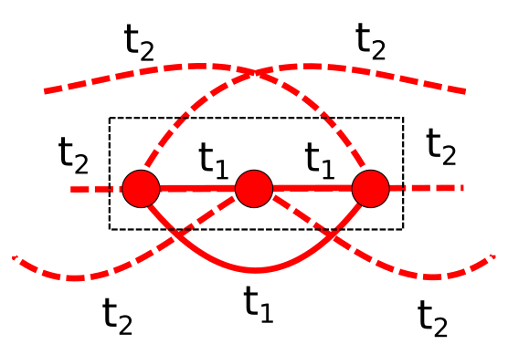
Figure 2.1: Translational symmetry in DMET. (a) The original lattice with translational symmetry, divided into 3 supercells. (b) The DMET fragment with broken intracluster translational symmetry, between the central site and the edge sites. (c) The DCA-DMET fragment restores the intracluster translational symmetry through a basis transformation and interaction coarse-graining.

Lattice DMET calculations with more than one orbitals in the fragment (referred as cluster DMET, or CDMET) suffers from broken intracluster translational symmetry due to the boundary effects (Fig. 2.1). The violence of translational symmetry causes conceptual and practical problems, such as the somewhat arbitrary measurement of observables in CDMET calculations. The dynamical cluster approximation (DCA) [120, 121, 122], originated from the DMFT community, defines a transformation of the lattice Hamiltonian such that the restriction to a finite fragment retains the periodic boundary within the fragment, thus restoring the intracluster translational symmetry (Fig. 2.1).

The DCA transformation involves two steps: a basis rotation which redefines the lattice one-body Hamiltonian, and a coarse graining of the two-body interaction [120, 121, 123, 124]. To introduce the DCA transformation, we first define the intra- and intercluster components of the real and reciprocal lattice vectors (Fig. 2.2),

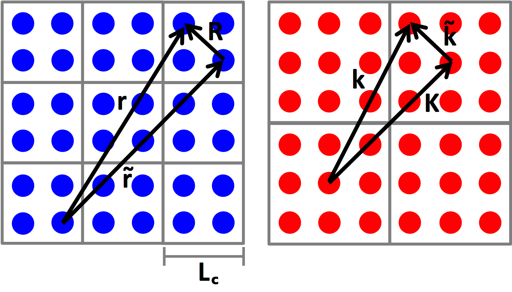
Figure 2.2: Definition of the real (left) and reciprocal (right) lattice vectors for the DCA transformation for a “hypercubic” fragment with $L_{c}=2$. The intercluster component of the real lattice vector, $\tilde{\mathbf{r}}$, labels the origin of the fragment, and the intracluster component, $\mathbf{R}$, labels the site within the fragment. The reciprocal space of $\tilde{\mathbf{r}}$ and $\mathbf{R}$ are labeled by $\tilde{\mathbf{k}}$ and $\mathbf{K}$, respectively.

$$\mathbf{r}=\mathbf{R}+\tilde{\mathbf{r}},\ \ \mathbf{k}=\mathbf{K}+\tilde{\mathbf{k}}.$$ (2.63)

For simplicity we assume “hypercubic” lattices (in arbitrary dimension) with orthogonal unit lattice vectors with linear dimension $L$, and “hypercubic” fragment with linear dimension $L_{c}$. The corresponding supercell lattice (of fragments) then has orthogonal lattice vectors of magnitude $L_{c}$, and the total number of supercells along each linear dimension is $L/L_{c}$.The intracluster lattice vector, $\mathbf{R}=(R_{1},R_{2},\cdots)$ and reciprocal lattice vector $\mathbf{K}=2\pi/L_{c}(N_{1},N_{2},\cdots)$ where $0\leq R_{i},N_{i}<L_{c};\ R_{i},N_{i}\in\mathbb{Z}$, and intercluster components $\tilde{\mathbf{r}}=L_{c}(\tilde{r}_{1},\tilde{r}_{2}\cdots)$, $\tilde{\mathbf{k}}=2\pi/L(\tilde{n}_{1},\tilde{n}_{2},\cdots)$, with $0\leq\tilde{r}_{i},\tilde{n}_{i}<L/L_{c};\ \tilde{r},\tilde{n}\in\mathbb{Z}$, are uniquely defined for any $\mathbf{r}$ and $\mathbf{k}$.

Our goal is to obtain a Hamiltonian which is jointly periodic in the intracluster and intercluster lattice vectors, $\mathbf{R}$ and $\tilde{\mathbf{r}}$. Such a jointly periodic basis is provided by the product functions $e^{-i\tilde{\mathbf{k}}\cdot\tilde{\mathbf{r}}}e^{-i\mathbf{K}\cdot{\mathbf{R}}}$. From one-body Hamiltonian $H_{1}$ defined in reciprocal space, $H_{1}=\sum_{\mathbf{k}}H_{1}(\mathbf{k})a_{\mathbf{k}}^{\dagger}a_{\mathbf{k}}$, and with the mapping in Eq. 2.63, we identify the diagonal DCA Hamiltonian matrix elements in the jointly periodic basis as

$$H_{1}(\mathbf{k})\to H_{1}^{\mathrm{DCA}}(\mathbf{\tilde{k},\mathbf{K}}).$$ (2.64)

The inverse Fourier transformation then gives the DCA matrix elements on the real-space lattice. The Fourier transforms between the different single particle Hamiltonians are summarized as:

$$\begin{split}H_{1}(\mathbf{r})&\xrightarrow[]{e^{-i\mathbf{k}\cdot\mathbf{r}}}H_{1}(\mathbf{k})\xrightarrow[]{\mathbf{k}=\tilde{\mathbf{k}}+\mathbf{K}}H_{1}^{\text{DCA}}(\tilde{\mathbf{k}},\mathbf{K})\\ &\xrightarrow[]{e^{i\tilde{\mathbf{k}}\tilde{\mathbf{r}}}}\xrightarrow[]{e^{i\mathbf{K}\cdot\mathbf{R}}}H_{1}^{\text{DCA}}(\tilde{\mathbf{r}},\mathbf{R}).\end{split}$$ (2.65)

The resultant real-space matrix elements, $H_{1}^{\text{DCA}}(\tilde{\mathbf{r}},\mathbf{R})$, thus only depend on the inter- and intracluster separation between sites. The transformation from $h(\mathbf{r})\to h_{\text{DCA}}(\tilde{\mathbf{r}},\mathbf{R})$ is simply a basis transformation of $h$, with the rotation matrix defined as [124]

$$C_{\mathbf{R}+\tilde{\mathbf{r}},\mathbf{R}^{\prime}+\tilde{\mathbf{r}}^{\prime}}=\sum_{\mathbf{K},\tilde{\mathbf{k}}}e^{-i[\mathbf{K}\cdot(\mathbf{R}^{\prime}-\mathbf{R})+\tilde{\mathbf{k}}(\tilde{\mathbf{r}}^{\prime}-\tilde{\mathbf{r}})+\tilde{\mathbf{k}}\cdot\mathbf{R}^{\prime}]}.$$ (2.66)

Viewing the DCA transformation as a basis rotation suggests that the same transformation should be extended to the interaction terms as well, generating nonlocal interactions. However, in DCA one uses a “coarse-grained” interaction in momentum space, which reduces the effect of nonlocal interactions to within the fragment [123]. The coarse-grained interaction is obtained by averaging the Fourier transformed interaction term over the intercluster reciprocal vectors for a given intracluster reciprocal vector.

A special case is the Hubbard model, where such coarse-graining leaves the local $Un_{i\alpha}n_{i\beta}$ term unchanged in the transformed Hamiltonian. Note that the coarse-grained Hubbard interaction is nonlocal if transformed back to the original site basis using the rotation in Eq. 2.66.

We can thus perform DMET using the DCA transformed Hamiltonian. To preserve intracluster translational symmetry of the DMET results, the correaltion potential $u_{C}$ is also required to be translational invariant within a fragment (See Appendix A.5). We refer this formulation as DCA-DMET. We present the numerical tests of DCA-DMET, as well as CDMET in Chapter 3.

2.5.3 Cluster Size Extrapolation 

As discussed in Sec. 2.3.3, extrapolation with the fragment size is an important tool to improve upon finite fragment DMET results. In this section, we present the theories of the cluster size scaling for energy and intensive observables. We analyze both CDMET and DCA-DMET in the Hubbard model on a $d$-dimensional hypercubic lattice, although most of the conclusions we derive here apply to other Hamiltonians as well. For the energy, we use a perturbation argument to obtain the leading term of the finite-size scaling; for the more complicated case of intensive observables, we suggest a plausible scaling form.

We consider the following factors to derive the DMET finite-size scaling for the Hubbard model: (a) the open boundary in CDMET; (b) the gapless spin excitations of quantum antiferromagnets; (c) the coupling between the impurity and bath; (d) the modification of the hoppings of the in DCA-DMET.

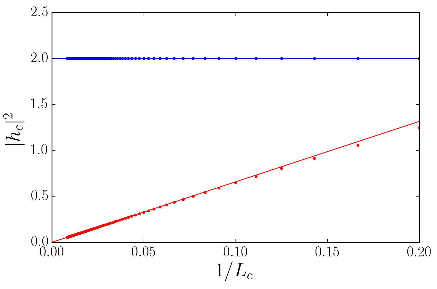
Figure 2.3: Sum-of-square of the one-body fragment-environment coupling Hamiltonian $|h_{c}|^{2}=\sum_{i\in C=0,j\in C^{\prime}\neq 0}|h_{ij}|^{2}$ for the CDMET and DCA-DMET formulations, in one-dimension. The fittings follow constant (CDMET) and $1/L_{c}$ (DCA) scalings, respectively.

We start with the CDMET energy. We first consider the bare fragment in CDMET (i.e. without the bath) which is just the finite size truncation of the infinite system. For a gapped system, we expect an open boundary to lead to a finite-size energy error (per site) proportional to the surface area to volume ratio [125], i.e.

$$e(L_{c})={e(\infty)}+\frac{a_{0}}{L_{c}}+\cdots$$ (2.67)

where $e(L_{c})$ is the energy per site for an $L_{c}^{d}$ site fragment and $e(\infty)$ is the energy per site in the thermodynamic limit (TDL). If, in the TDL, there are gapless modes, a more careful analysis is required. The Hubbard model studied here has gapless spin excitations. These yield a finite size error of $O(1/L_{c}^{d+1})$ in a fragment with periodic boundary condition (PBC) [126, 127, 128, 129], which is subleading to the surface finite size error introduced by the open boundary in Eq. 2.67 for $d>0$.

We next incorporate the CDMET bath coupling. Each site on the fragment boundary couples to the bath, yielding a total Hamiltonian coupling of $O(1)$ per boundary site (see Fig. 2.3). The total “perturbation” to the bare fragment Hamiltonian is then $O(L_{c}^{d-1})$, which leads to a first order energy correction per site. Thus, in CDMET, the open boundary and the error in the bath orbitals together cause the leading contribution to the finite size error

$${e(L_{c})_{\text{CDMET}}}={e(\infty)}+\frac{a_{0}^{\prime}}{L_{c}}+\cdots$$ (2.68)

in any dimension.

For DCA-DMET, the above argument must be modified in two ways: first, the fragment uses PBC, and second, the formulation modifies intercluster and intracluster hoppings. Similarly, we start with the bare periodic fragment (without any modification of the intracluster hoppings).

In the TDL, for a gapped state with short-range interactions, all correlation functions decay exponentially (e.g. Wannier functions are exponentially localized) and we expect an exponential convergence of the energy with respect to fragment size.

However, in the Hubbard model, as previously mentioned, the gapless spin excitations give a finite-size energy error (per site) of $O(1/L_{c}^{d+1})$. The leading order finite-size scaling for the bare periodic fragment is thus expected to be

$$e(L_{c})=e(\infty)+\frac{a_{0}}{L_{c}^{d+1}}+\cdots.$$ (2.69)

The DCA-DMET Hamiltonian modifies the periodic fragment Hamiltonian by changing both the intracluster and intercluster hopping terms. The intracluster hopping terms are modified by a term of order $O(1/L_{c}^{2})$, and the intercluster hopping terms are modified so as to generate a coupling between each site in the fragment and the bath with a total interaction strength of $O(1/L_{c}^{2})$ (see Fig. 2.3). Since there are $L_{c}^{d}$ sites in the fragment, the total magnitude of the DCA-DMET perturbation (including the contributions of both intracluster and intercluster terms) is $O(L_{c}^{d-2})$.

For one dimension, the perturbation and fragment-bath coupling give a contribution with the same scaling as the contribution of the gapless modes, while in two and higher dimensions, they give the leading term in the finite-size error. Thus combining the three sources of finite-size error we expect in any dimension the energy per site scaling of DCA-DMET to be

$$e(L_{c})_{\text{DCA-DMET}} ={e(\infty)}+\frac{a_{0}^{\prime}}{L_{c}^{2}}+\cdots.$$ (2.70)

Note that the scaling of the CDMET and DCA-DMET energies is the same as is found for CDMFT and DCA.

The finite size scaling of intensive quantities is more tricky to analyze [130]. For an observable $Q$ we have the relation $\langle Q\rangle=\lim_{r\to\infty}\langle Q(0)Q(r)\rangle^{1/2}$, where $\langle Q(0)Q(r)\rangle$ is the correlation function. It is often argued that the error in $\langle Q\rangle$ in a large finite fragment behaves like

$$\Delta Q\sim[\langle Q(0)Q(R)\rangle^{1/2}-\langle Q(0)Q(\infty)\rangle^{1/2}]$$ (2.71)

where $R$ is the largest length in the fragment [128] $\sim L_{c}/2$. For CDMET, where the cluster is only coupled to the symmetry-broken bath at the boundary, we assume the form in Eq. 2.71 holds, with additional corrections from the fragment size, expanded as a Taylor series

$$\Delta Q(L_{c})=\left(a+\frac{b}{L_{c}}+\cdots\right)[\langle Q(0)Q(R)\rangle^{1/2}-\langle Q(0)Q(\infty)\rangle^{1/2}].$$ (2.72)

Eq. 2.72 is a heuristic form and its correctness will be assessed in our numerical results in Chapter 3. Taking the local magnetic moment $m=\langle S_{z}\rangle$ as an example, the correlation function $\langle S_{z}(0)S_{z}(r)\rangle$ at large $r$ behaves like $a\sqrt{\ln r}/r$ in the 1D Hubbard model, and $a+b/r$ in the 2D square-lattice Hubbard model at half-filling. Consequently, we can assume a scaling form in 1D of

$$m(L_{c})_{\text{CDMET}}=\sqrt{\frac{\sqrt{\ln L_{c}/2}}{L_{c}/2}}\left(a+\frac{b}{L_{c}}+\cdots\right)$$ (2.73)

and in 2D of

$$m(L_{c})_{\text{CDMET}}=a+\frac{b}{L_{c}}+\frac{c}{L_{c}^{2}}+\cdots.$$ (2.74)

For DCA-DMET, however, every fragment site, not just those at the boundary, is coupled to a set of bath orbitals, which provides a symmetry-breaking pinning field. This means that there is no simple connection to the scaling of correlation function (with respect to distance) of the system. Thus, there is no obvious theoretical argument for any form of scaling for the observables in DCA-DMET, and we can, at best, assume the Taylor expansion in both one- and two-dimensions,

$$m(L_{c})_{\text{DCA-DMET}}=a+\frac{b}{L_{c}}+\frac{c}{L_{c}^{2}}+\cdots.$$ (2.75)

Chapter 3 Cluster Size Convergence of the Density Matrix Embedding Theory and Its Dynamical Cluster Formulation 

We present in this chapter the numerical studies of cluster size convergence of the energy and observables using two forms of DMET: the original CDMET and the DCA-DMET, motivated by the dynamical cluster approximation (see Sec. 2.5.2). Both methods are applied to the half-filled one- and two-dimensional Hubbard models using a sign-problem free AFQMC impurity solver (see Sec. 2.4.3), which allows for the treatment of large impurity clusters of up to 100 sites. While CDMET is more accurate at smaller fragment sizes, DCA-DMET exhibits faster asymptotic convergence towards the TDL. In addition to investigating the cluster size convergence scaling, these calculations produce accurate estimates for the energy and local moment of the two-dimensional Hubbard model for $U/t=2,4,6$. The results compare favorably with the best data available in the literature, and help resolve earlier uncertainties in the moment for $U/t=2$.

In Sec. 3.1, we introduce the background and motivation of the study. In Sec. 3.2, we briefly describe the methods and parameters used in the calculations. We present the calculation results in Sec. 3.3 and discuss the implications of the results in Sec. 3.4.

3.1 Introduction

An critical dimension in numerical studies of lattice models is the ability to study the physical properties in TDL. To do so, one typically considers finite sized clusters of increasing sizes under some choice of boundary conditions, followed by a finite size scaling of the observables. Embedding methods accelerate the finite size convergence, by mapping the bulk problem onto an auxiliary impurity model, where a small fragmen of the physical interacting sites is coupled to special “bath sites” that mimic the effects of the neglected environment.

As discussed in Sec. 2.3.3, the cluster size extrapolation is a great tool to extend the scope of DMET studies. A detailed analysis of the finite-size scaling of DMET not only is theoretically interesting, but helps obtaining accurate TDL estimates in all future DMET studies.

In this chapter, we perform such a detailed investigation in the context of the half-filled 1D and 2D square lattice Hubbard models using the AFQMC impurity solver, implemented by Zhang, et. al. [103, 104]. Because of the absence of the sign problem, these models serve as an excellent testing bed for the purpose, as we are able to study DMET fragments with up to 100 fragment sites. Using this solver further facilitates direct comparisons to bare (i.e. not embedded) AFQMC calculations in the literature that used very large clusters (with up to 1058 sites) with periodic (PBC), anti-periodic (APBC), modified (MBC), and twisted boundary (TBC) conditions  [3, 1]. The comparison provides a direct demonstration of the benefits of embedding, versus simply modifying the boundary conditions.

Similar to previously established scalings for CDMFT and DCA  [125, 130, 131, 132, 133], the CDMET and DCA-DMET converge $O(1/L_{c})$ and $O(1/L_{c}^{2})$ from the theoretical analysis (Sec. 2.5.3). In this chapter, we perform CDMET and DCA-DMET calculations on 1D and 2D Hubbard model at half-filling for $U/t=4,8$ and $U/t=2,4,6$, respectively, to confirm the scalings of the TDL energies and to investigate the convergence of the TDL spin-moments.

For the energies, our results provide high accuracy benchmarks with small error bars. Converging finite-size effects for spin-moment has well-known pitfalls, and existing data in the literature do not always agree  [5, 6, 2, 3, 1]. Where an agreement is observed, our new estimates confirm the existing data with comparable or improved error bars. In the case of $U/t=2$ where severe finite size effects are found, our data resolves between the earlier incompatible estimates in the literature.

3.2 Methods

The Hubbard Hamiltonian is defined as

$$H=-t\sum_{\langle ij\rangle\sigma}a_{i\sigma}^{\dagger}a_{j\sigma}+\sum_{i}Un_{i\alpha}n_{i\beta}$$ (3.1)

where $a_{i\sigma}^{\dagger}$ ($a_{i\sigma}$) creates (destroys) a particle of spin $\sigma$ at site $i$, $\langle ij\rangle$ denotes nearest neighbors, and $n_{i\sigma}=a_{i\sigma}^{\dagger}a_{i\sigma}$.

We apply the standard spin-unrestricted, normal state CDMET algorithm detailed in Appendix B.1 to the Hubbard models, with the following modifications: (i) the correlation potential is restricted to preserve the particle-hole symmetry so that the AFQMC impurity solver does suffer from the sign problem (Eq. 2.57); and (ii) the chemical potential fitting is skipped since $\mu\equiv U/2$ at half-filling.

The DCA-DMET calculations are performed similarly with the modified Hamiltonian described in Sec. 2.5.2, which restores intracluster translational symmetry. There is also stronger restrictions on the correlation potential in DCA-DMET, as it preserves both the translational and the particle-hole symmetry.

In the calculations of this chapter, we use the AFQMC impurity solver, whose implementation described in Refs. [104, 105, 106] with small modifications to treat Hamiltonians with broken $S^{2}$ symmetry  . Both the energy and the one-body density matrix (required for the DMET self-consistency) are computed by the pure estimator, Eq. 2.56. We converge the standard deviation of all elements in the one-body density matrix to be less than 0.001, to make the AFQMC statistical errors (and thus DMET statistical convergence errors) orders of magnitude smaller than the finite cluster size error. This results in considerably higher statistical accuracy for extensive quantities than typically obtained in the AFQMC literature.

The finite fragment results are extrapolated to obtain TDL estimates following the scalings suggested by the theoretical analysis in Sec. 2.5.3. The quality of these extrapolations is assessed.

3.3 Results

We present the CDMET and DCA-DMET calculations on the half-filled 1D and 2D Hubbard models, focusing on the finite-size convergence of the energy and local observables. As discussed in section 3.2 the DMET correlation potential preserves $S_{z}$ symmetry but is allowed to break $S^{2}$ symmetry. For the Hubbard models studied here, all the converged self-consistent DMET solutions explicitly break $S^{2}$ symmetry.

In 1D, we compare our results against exact results from the Bethe Ansatz (BA), while in 2D, we compare to literature benchmark data from AFQMC calculations scaled to the TDL [6, 3, 1], DMRG calculations scaled to the TDL [2], and iPEPS calculations scaled to zero truncation error [4].

3.3.1 1D Hubbard Model

We study fragment clusters with $N_{\text{imp}}=L_{c}\leq 24$ sites on a DMET auxiliary lattice with $N=L=480$ (even $N_{c}$) or $N=L=480+L_{c}$ (odd $N_{c}$) sites. The auxiliary lattice uses PBC, and as the DCA-DMET impurity Hamiltonian becomes complex for even $N_{c}$, we only use auxiliary lattices with an odd $N_{c}$ in the DCA-DMET calculations. We study two couplings $U/t=4$ (moderate coupling) and $U/t=8$ (strong coupling). When starting from uniform antiferromagnetic initial guesses for the correlation potential, it usually takes 4 to 8 DMET iterations to converge the calculations.

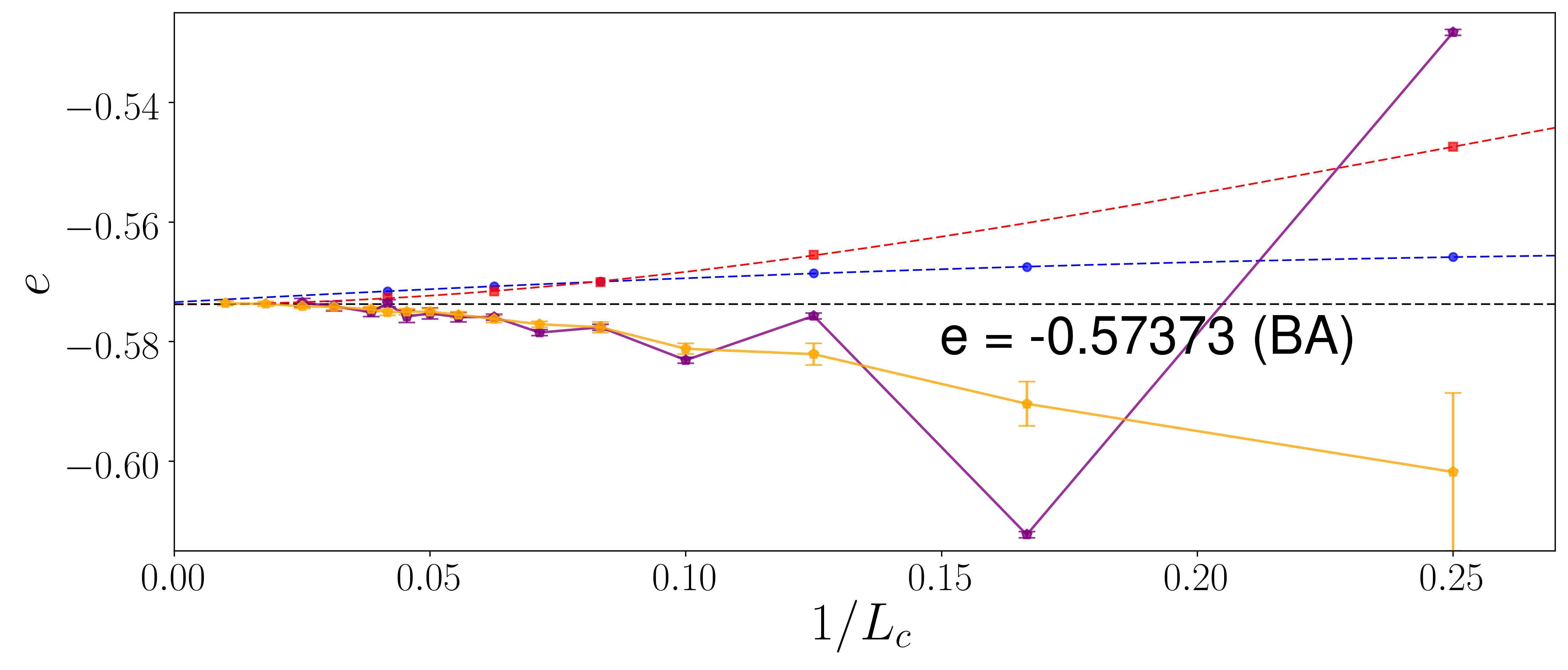
(a) U/t = 4

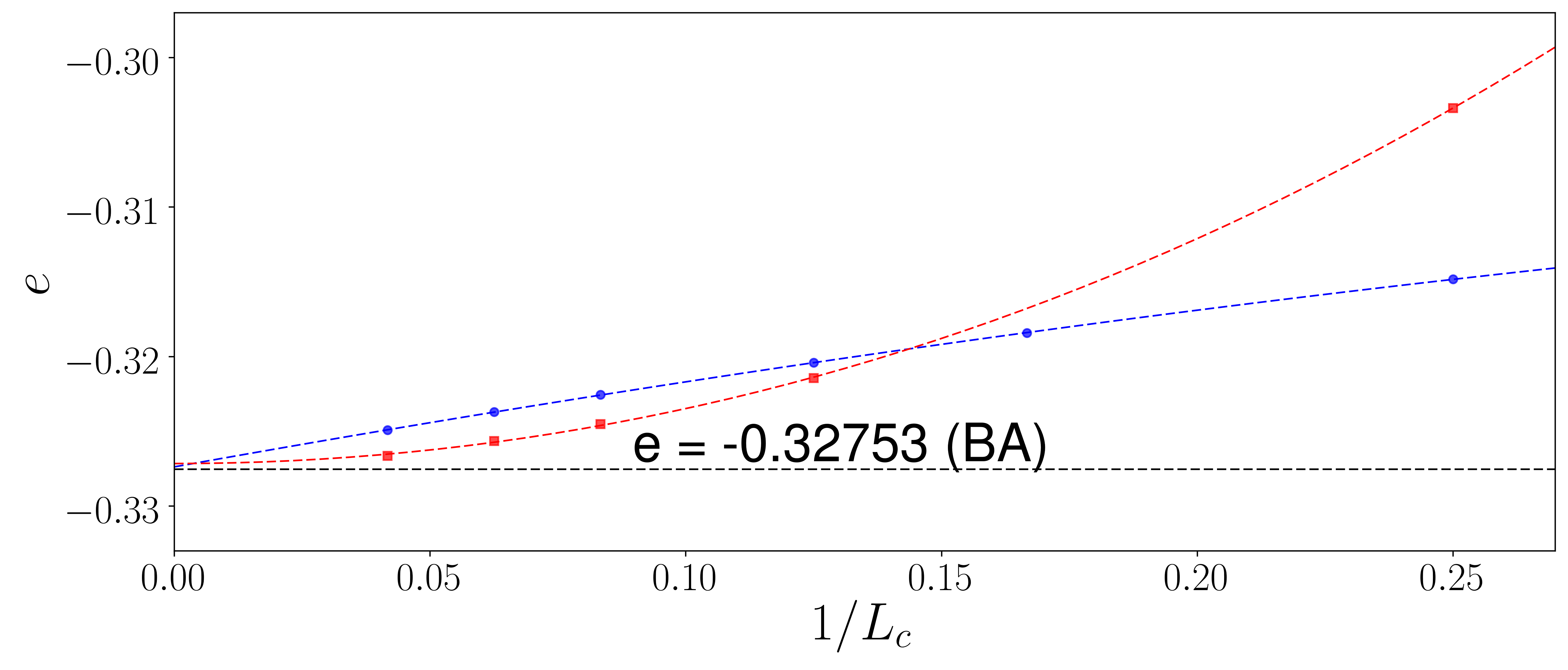
(b) U/t = 8

Figure 3.1: Energy per site, $e$, for the half-filled 1D Hubbard model versus inverse impurity size, $1/L_{c}$, from CDMET (blue) and DCA-DMET (red). For comparison, we also plot the same numbers from AFQMC with PBC (purple) and TABC (orange) for $U/t=4$. The extrapolations use $e=a+bL_{c}^{-1}+cL_{c}^{-2}$ for CDMET and $e=a+bL_{c}^{-2}+cL_{c}^{-3}$ for DCA-DMET.

Fig. 3.1 shows the energy per site as a function of inverse impurity size $1/L_{c}$. Statistical error bars associated with the AFQMC solver are not shown here as they are too small to be visible; this is true for all the CDMET and DCA-DMET results presented in this chapter. As shown in Table 3.1, the extrapolated energies are in generally good agreement with the exact Bethe ansatz TDL data, with a deviation of less than $0.001t$. To further improve the accuracy, we include the subleading terms in the energy extrapolation, i.e. $a+b/L_{c}+c/L_{c}^{2}$ for CDMET and $a+b/L_{c}^{2}+c/L_{c}^{3}$ for DCA-DMET (dashed lines in Fig. 3.1). This improves the extrapolated TDL results significantly, with the single exception of DCA-DMET at $U/t=8$, where the coefficient of the cubic term is not statistically significant [$c=0.08(9)$] and the deviation is already very small. The subleading terms are more important at $U/t=4$ than at $U/t=8$. This is consistent with the smaller gap at weaker coupling, that introduces stronger finite size effects.

Table 3.1: CDMET and DCA-DMET cluster size extrapolation of the energy per site (in units of $t$) for the 1D half-filled Hubbard model.

Extrapolation		$\mathbf{U/t=4}$	$\mathbf{U/t=8}$
CDMET	$a+b/L_{c}$	-0.5724(3)	-0.3267(2)
	$a+b/L_{c}+c/L_{c}^{2}$	-0.5734(1)	-0.3274(1)
DCA-DMET	$a+b/L_{c}^{2}$	-0.5729(4)	-0.3273(1)
	$a+b/L_{c}^{2}+c/L_{c}^{3}$	-0.5738(1)	-0.3272(1)
Bethe Ansatz		-0.57373	-0.32753

To further numerically test the scaling form for the DCA-DMET extrapolation, we include a linear $1/L_{c}$ term in the DCA-DMET scaling form, i.e. $a+b/L_{c}+c/L_{c}^{2}$. While the coefficient of the linear term is statistically significant at $U/t=4$, the extrapolated TDL energy acquires a larger uncertainty [-0.5749(6)], while for $U/t=8$, the coefficient of $1/L_{c}$ term becomes statistically insignificant [$b=0.003(5)$]. This supports the leading finite-size scaling of the DCA-DMET energy per site as being $O(1/L_{c}^{2})$. The finite size scaling of the energy observed for CDMET and DCA-DMET is consistent with similar data observed for CDMFT and DCA [130, 123].

In Fig. 3.1(a), we plot the AFQMC results with periodic (PBC) and twist-average (TABC) boundary conditions as well. While the PBC energy oscillates strongly for all cluster sizes, the convergence of TABC is much smoother. The finite-size scaling of bare cluster AFQMC (PBC and TABC) appears to be quadratic in inverse size, which is consistent with the spin-wave theory predictions in 1D [128], and coincides with the scaling of DCA-DMET. Therefore, with large clusters, the finite-size errors of bare cluster AFQMC and DCA-DMET are comparable and smaller than those of CDMET, while CDMET is much more accurate for small fragments.

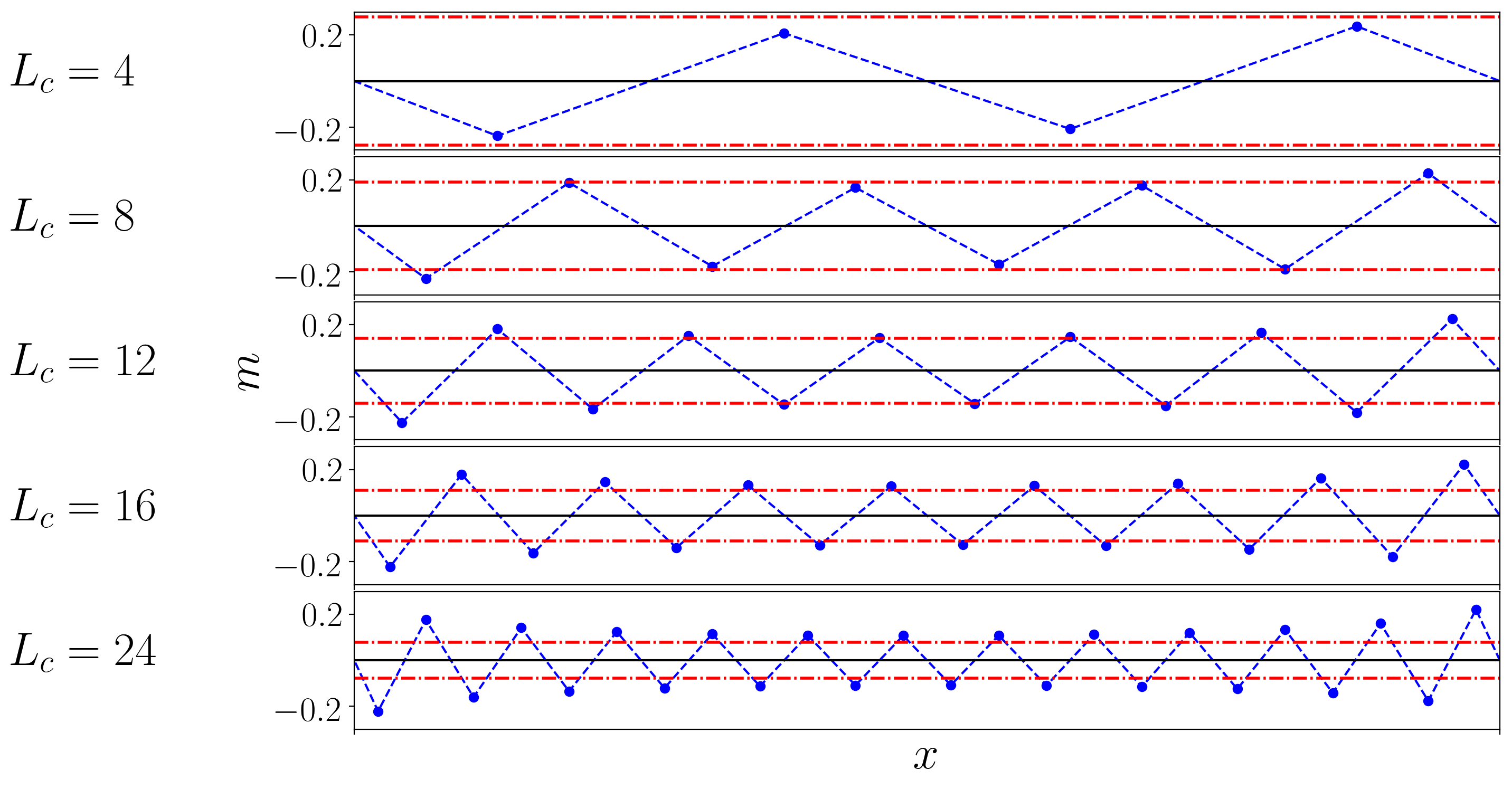
Figure 3.2: Local spin moments $m$ from CDMET (blue) and DCA-DMET (red) in finite fragment calculations at $U/t=4$ in the 1D Hubbard model. $x$ is the site index scaled to the interval $[0,1]$ for the CDMET results.

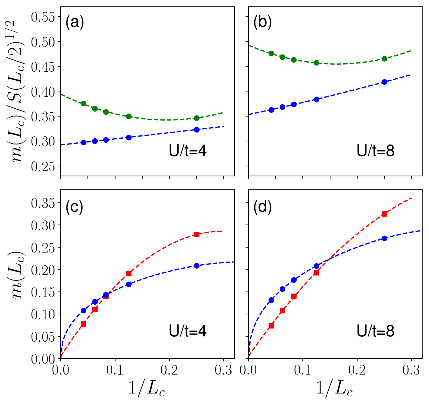
Figure 3.3: Cluster size extrapolation of the AF order parameters in the 1D Hubbard model. (a) (b) CDMET AF order parameters $m(L_{c})$ divided by spin correlation function $S(L_{c}/2)^{1/2}$, versus inverse impurity cluster size $1/L_{c}$ for $U/t=4$ and $U/t=8$ (blue: center average, green: entire cluster average). The extrapolation uses the form $m(L_{c})/S(L_{c}/2)^{1/2}=a+bL_{c}^{-1}+cL_{c}^{-2}$, see Eq. 2.73 for details. (c) (d) DCA-DMET and CDMET (center average) AF order parameters $m(L_{c})$ versus inverse impurity cluster size $1/L_{c}$ for $U/t=4$ and $U/t=8$. The extrapolation for DCA-DMET values uses the form $m(L_{c})=a+bL_{c}^{-1}+cL_{c}^{-2}$, see Eq. 2.75 for details.

We now turn to the spin orders. Although there is no true long-range antiferromagnetic (AF) order in 1D, the finite correlated fragment calculations yield non-zero spin moments, which should extrapolate to zero in the TDL. The local spin moments $m$ are plotted in Fig. 3.2. We see that the spin moments in the CDMET fragment are largest at the boundary with the AF environment, and decay towards the center. We can understand this because quantum fluctuations are incompletely treated in the bath orbitals, and thus they are overmagnetized. This effect is propagated to the boundary of the CDMET fragment. Note that the fragment sites in a DCA-DMET cluster are all equivalent, and are equally coupled to the environment, resulting in an equal spin magnitude for all sites, to within the statistical error of the solver. In Fig. 3.2 we use the two horizontal lines to represent the spin magnitudes from the DCA-DMET calculations.

To determine the magnetic order parameter from CDMET, we consider two possible definitions: (a) the average $|m|$ for the central pair (or the plaquette in 2D); (b) the average $|m|$ over the entire fragment. These definitions are equivalent for DCA-DMET. In CDMET, they agree in the limit of small clusters ($L_{c}=2$) and large clusters ($L_{c}\rightarrow\infty$), but differ inbetween.

The AF order parameters for different fragment sizes are plotted in Figs. 3.3 for different $U$. For CDMET, we fit the order parameter to the scaling form in Eq. 2.73, up to second order. The fits are shown in Figs. 3.3(a), (b), and are quite good for both types of measurements. For the average $|m|$ of the central pair, an almost straight line is observed at both couplings, with the quadratic term close to vanishing ($c=0.00(4)$ for $U/t=4$ and $c=0.12(7)$ for $U/t=8$). The average $|m|$ over the entire fragment requires a larger $c$ for a good fit. This is because $|m|$ is measured at different points which corresponds to averaging over different effective lengths $L_{c}$ in Eq. 2.73. Averaging over Eq. 2.73 yields the same leading scaling but introduces larger subleading terms. Overall, the error decreases much more rapidly by using the center average, consistent with observations in CDMFT [133].

For DCA-DMET, the scaling form Eq. 2.75 truncated at second order works well. This correctly predicts the vanishing local moments at the TDL ($a=0.005(1)$ at $U/t=4$ and $a=0.005(4)$ at $U/t=8$). The $O(1/L_{c})$ scaling of DCA-DMET thus converges faster than CDMET, whose leading term is $\left(\frac{\sqrt{\log(L_{c}/2)}}{L_{c}/2}\right)^{1/2}\sim L_{c}^{-1/2}$.

While the smallest fragments in CDMET report a smaller magnetization than seen in DCA-DMET (and thus can be regarded as “closer” to the TDL) the cross-over between the DCA-DMET and CDMET moments occurs at smaller clusters than for the energy.

3.3.2 2D Hubbard Model

We now show results from the half-filled 2D Hubbard model at $U/t=2,4,6$. We use square fragments of size $N_{\textrm{imp}}=L_{c}\times L_{c}$, where for CDMET $L_{c}=2,4,6,8,10$ and for DCA-DMET $L_{c}=4,6,8,10$. The $2\times 2$ plaquette is not used in the finite-size scaling of DCA-DMET as it is known from DCA studies to exhibit anomalous behavior [130], which we also observe. Also at $U/t=6$, we do not present results for $L_{c}=10$, as we are unable to converge the statistical error to high accuracy in the AFQMC calculations (within our computational time limits). The total lattices we used have linear lengths of around $L=120$ ($N=L\times L$), adjusted to fit even (CDMET) or odd (DCA-DMET) $N_{c}$, as in the 1D case. As in 1D, we initialize the correlation potential as a diagonal matrix with uniform AF terms. The 2D calculations thus take slightly more self-consistent iterations (about 10) than in 1D to converge.

In Fig. 3.4, we show the cluster size dependence of the energy per site; the data is tabulated in Table 3.2. Because there are no exact TDL results for the 2D Hubbard model, we show gray ribbons as “consensus ranges”, obtained from the TDL estimates of several methods including (i) AFQMC extrapolated to infinite size [3, 1], (ii) DMRG extrapolated to infinite size [2], and (iii) iPEPS extrapolated to zero truncation error [4]. To show the effects of embedding versus bare cluster AFQMC calculations we also plot the AFQMC results of Ref. [1] on finite lattices with up to 400 sites, using TABC for $U/t=2,4,6$, as well as periodic (PBC) and anti-periodic (APBC) boundary conditions for $U/t=4$.

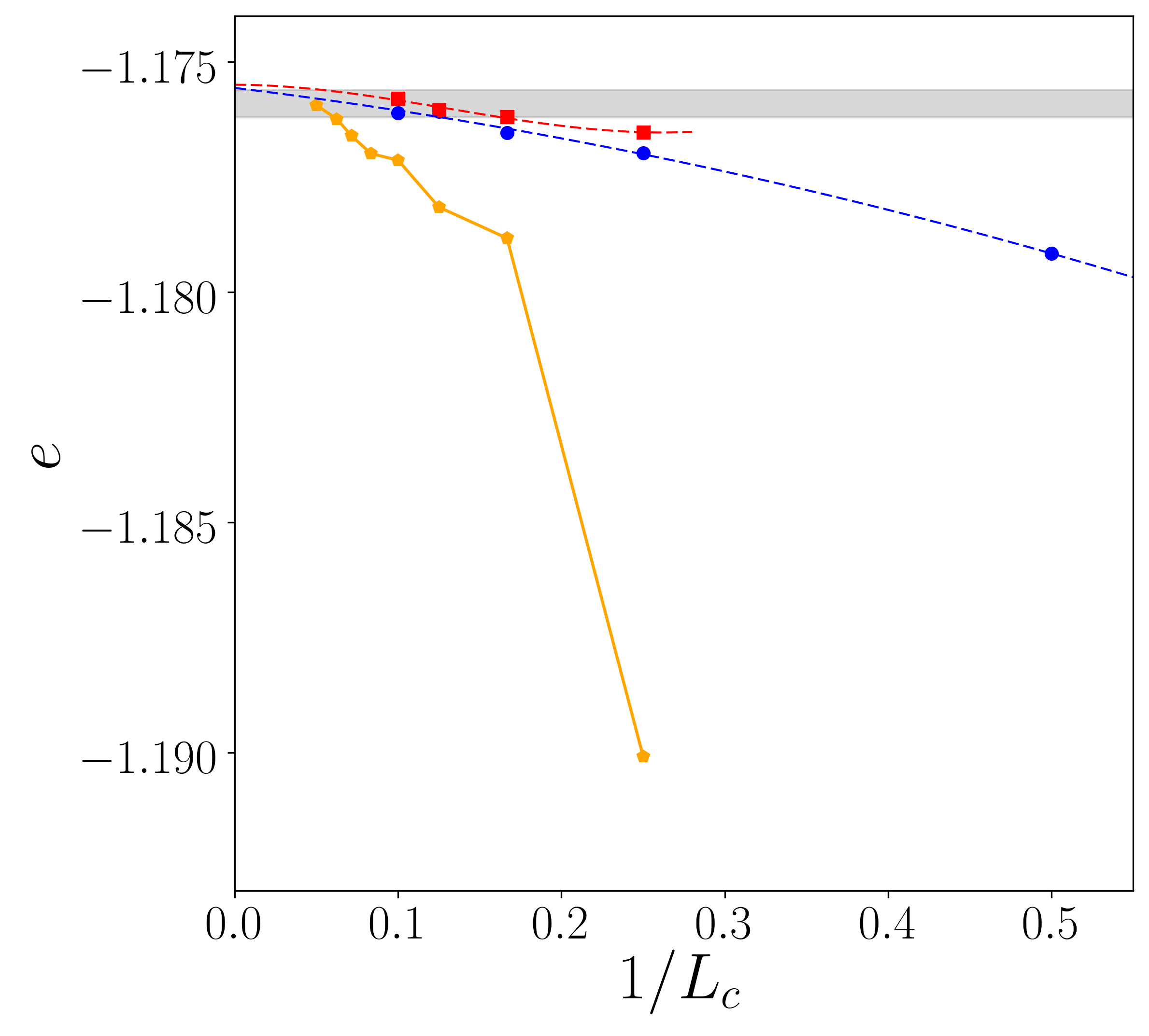
(a) U/t = 2

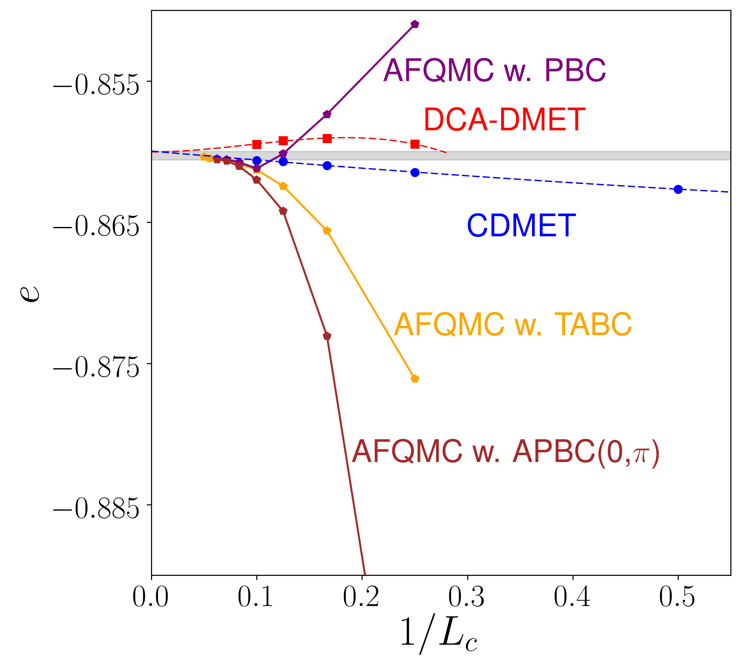
(b) U/t = 4

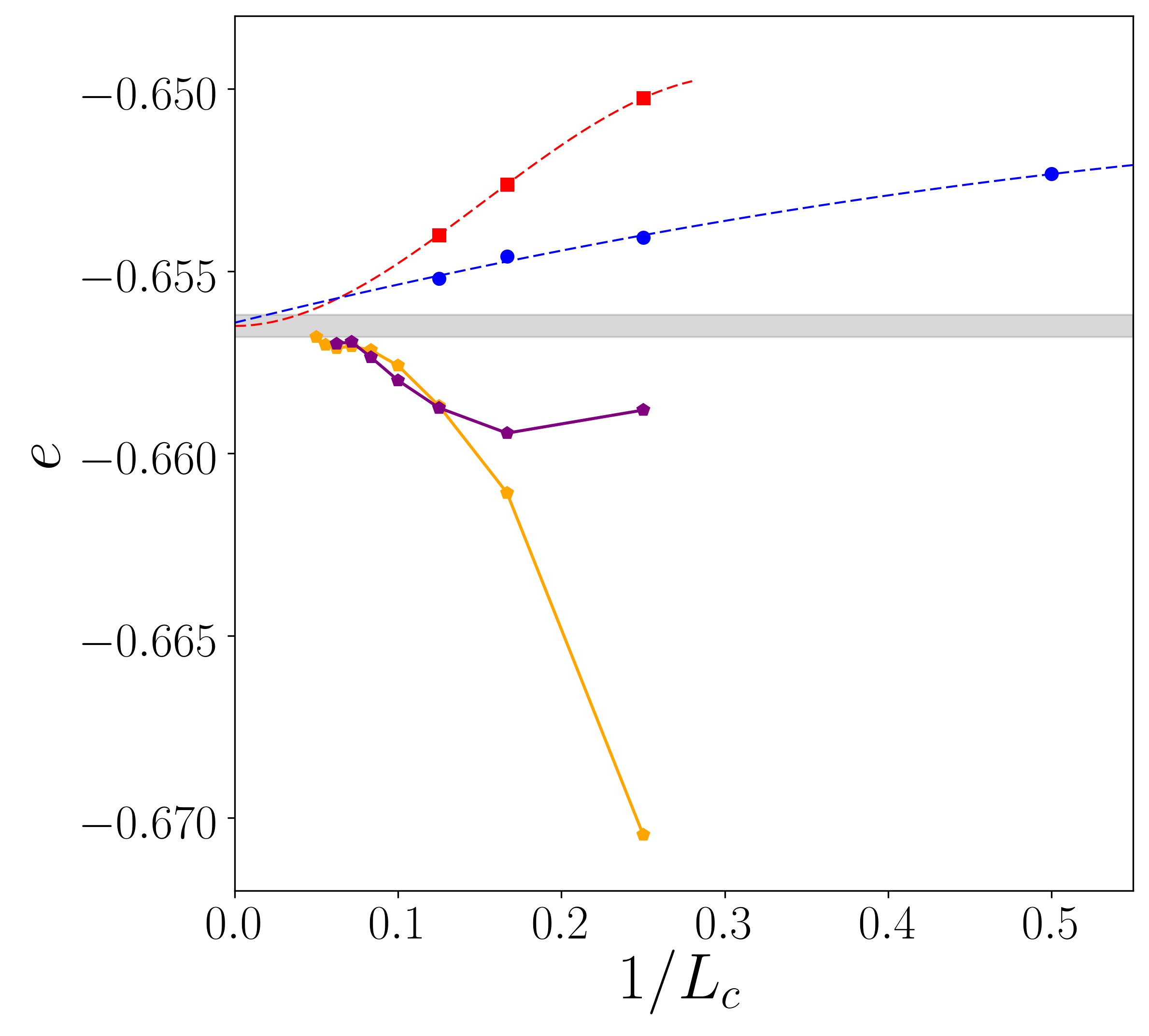
(c) U/t = 6

Figure 3.4: Energy per site $e$ versus $1/L_{c}$ in the 2D Hubbard model from CDMET (blue), DCA-DMET (red) and finite system AFQMC (orange: TABC, purple: PBC, brown: APBC for y-direction and PBC for x-direction) (from Ref. [1]). The consensus range illustrated by the grey-shaded region represents the TDL results of AFQMC, DMRG and iPEPS calculations in Refs. [2, 3, 4, 1].

In 2D, both CDMET and DCA-DMET appear to display much higher accuracy for small fragments, compared to in 1D. Although DMET is not exact in the infinite dimensional limit, this is similar to the behavior of DMFT, which improves with increasing coordination number [44]. The DMET energies for each fragment size are, as expected, much closer to the TDL estimates than the finite system AFQMC energies, even when twist averaging is employed to reduce finite size effects. For example, the $2\times 2$ CDMET energy is competitive with the $8\times 8$ AFQMC cluster energy with twist averaging. Further, the convergence behavior generally appears smoother in DMET than with the bare clusters, likely due to smaller shell filling effects. Combining these benefits, we find that using DMET gives several orders of magnitude savings in computation time to achieve a given energy accuracy in the TDL estimate, as compared to using bare cluster calculations alone. This illustrates the benefits of using bath orbitals to approximately represent the environment in an embedding.

Table 3.2: Finite size extrapolation of the energy for the 2D half-filled Hubbard model.

Methods		$\mathbf{U/t=2}$	$\mathbf{U/t=4}$	$\mathbf{U/t=6}$
CDMET	$a+b/L_{c}$	-1.1752(1)	-0.8601(1)	-0.6560(2)
	$a+b/L_{c}+c/L_{c}^{2}$	-1.1756(3)	-0.8600(1)	-0.6564(6)
DCA-DMET	$a+b/L_{c}^{2}$	-1.1758(1)	-0.8593(2)	-0.6550(4)
	$a+b/L_{c}^{2}+c/L_{c}^{3}$	-1.1755(2)	-0.8600(2)	-0.6565a
AFQMC	TABC [1]	-1.1760(2)	-0.8603(2)	−0.6567(3)
	MBC [3]	-1.17569(5)	-0.86037(6)	-
DMRG [2]		-1.176(1)	-0.8605(5)	-0.6565(1)
iPEPS [4]		-	-0.8603(5)	-
Consensus range		-1.1758(3)	-0.8603(3)	-0.6565(3)

$a$ Uncertainty cannot be computed due to insufficient data points in the fit.

We now discuss our TDL estimates. As in the 1D Hubbard model, we use the scaling forms proposed in Sec. 2.5.3, i.e. $a+b/L_{c}(+c/L_{c}^{2})$ for CDMET and $a+b/L_{c}^{2}(+c/L_{c}^{3})$ for DCA-DMET. The results are summarized in Table 3.2 and plotted in Fig. 3.4. The TDL energy estimates fall within the TDL consensus range, with an error bar competitive with the best large-scale ground state calculations. The DMET estimates are also all in agreement (within 2$\sigma$) of our earlier CDMET extrapolations that only used fragments of up to $4\times 4$ sites in Refs. [92, 2]. The largest deviation from our earlier small fragment DMET extrapolations is for $U/t=2$ where finite size effects are strongest; the current estimates of $-1.1756(3)$ (CDMET) and $-1.1755(2)$ (DCA-DMET) can be compared with our small fragment estimate of $-1.1764(3)$, and the recent TDL estimate of Sorella of $-1.17569(5)$, obtained by extrapolating AFQMC energies from clusters as large as 1058 sites, using modified (periodic) boundary conditions [3]. Note that the subleading terms are more important for accurate extrapolations in 2D than they are in 1D. This is simply because we do not reach as large linear dimensions in 2D as in 1D, which means that we are not fully in the asymptotic regime. For the same reason it is more difficult to see the crossover between the convergence of DCA-DMET and CDMET. For $U/t=2$, it appears advantageous to use the DCA-DMET formulation already for fragments of size $L_{c}\geq 4$, while at $U/t=4,6$ it appears necessary to go to fragments larger than the largest linear size used in this study, $L_{c}=10$.

Table 3.3: Estimated staggered magnetization for the 2D half-filled Hubbard model at TDL.

Methods	$\mathbf{U/t=2}$	$\mathbf{U/t=4}$	$\mathbf{U/t=6}$
CDMET	0.115(2)	0.226(3)	0.275(8)
DCA-DMET	0.120(2)	0.227(2)	0.261a
DQMC [5]	0.096(4)	0.240(3)	0.283(5)
Pinning field QMC [6]	0.089(2)	0.215(10)	0.273(5)
AFQMC w. TABC [1]	0.119(4)	0.236(1)	0.280(5)
AFQMC w. MBC [3]	0.120(5)	-	-

$a$ Uncertainty cannot be computed due to insufficient data points in the fit.

The AF order in the half-filled 2D Hubbard model is long-ranged in the ground state. In the left part of Fig. 3.5, the AF order parameters from DMET finite fragment calculations are plotted and extrapolated, with the right panel showing comparisons of TDL estimates with the other methods. In addition, we summarize the extrapolated TDL estimates for the AF order parameters in Table. 3.3. For CDMET, the order parameters are measured as the average magnitude of the central plaquette. We fit the magnetization data to the form suggested in Section 2.5.3, i.e. $a+b/L_{c}+c/L_{c}^{2}$ for both CDMET and DCA-DMET. These fits lead to good agreement between the CDMET and DCA-DMET TDL estimates, supporting the scaling form used. At $U/t=4$, the CDMET and DCA-DMET TDL moments are in good agreement with the estimates from two different AFQMC calculations, with competitive error bars. At $U/t=6$, the CDMET TDL moment is consistent with the two AFQMC estimates although the DCA-DMET estimate is somewhat smaller than the two AFQMC estimates. (We do not have errors bars for the $U/t=6$ DCA-DMET moment as we are fitting 3 data points to a 3 parameter fit).

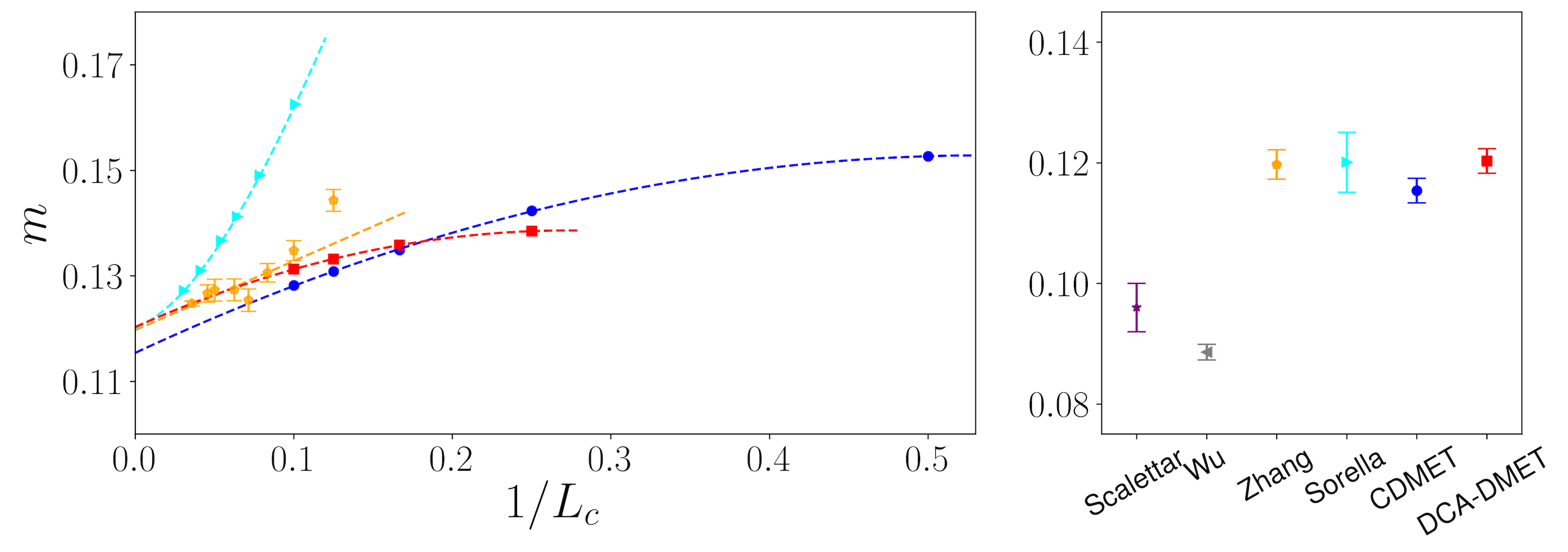
(a) U/t = 2

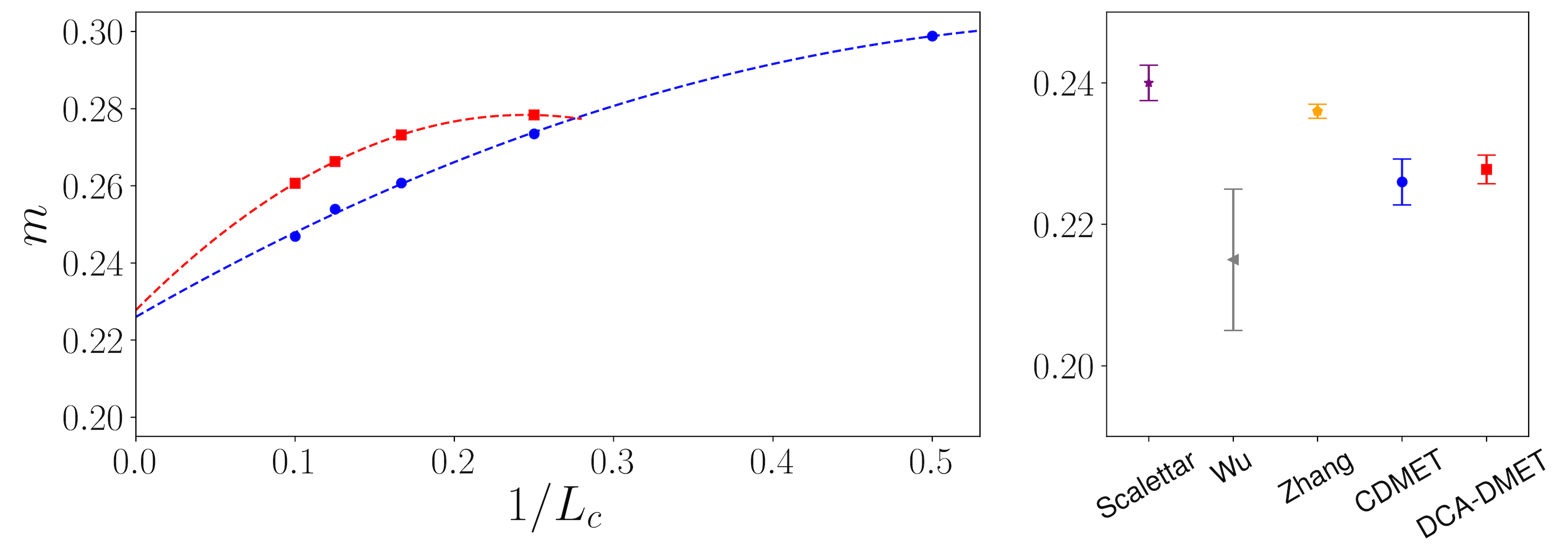
(b) U/t = 4

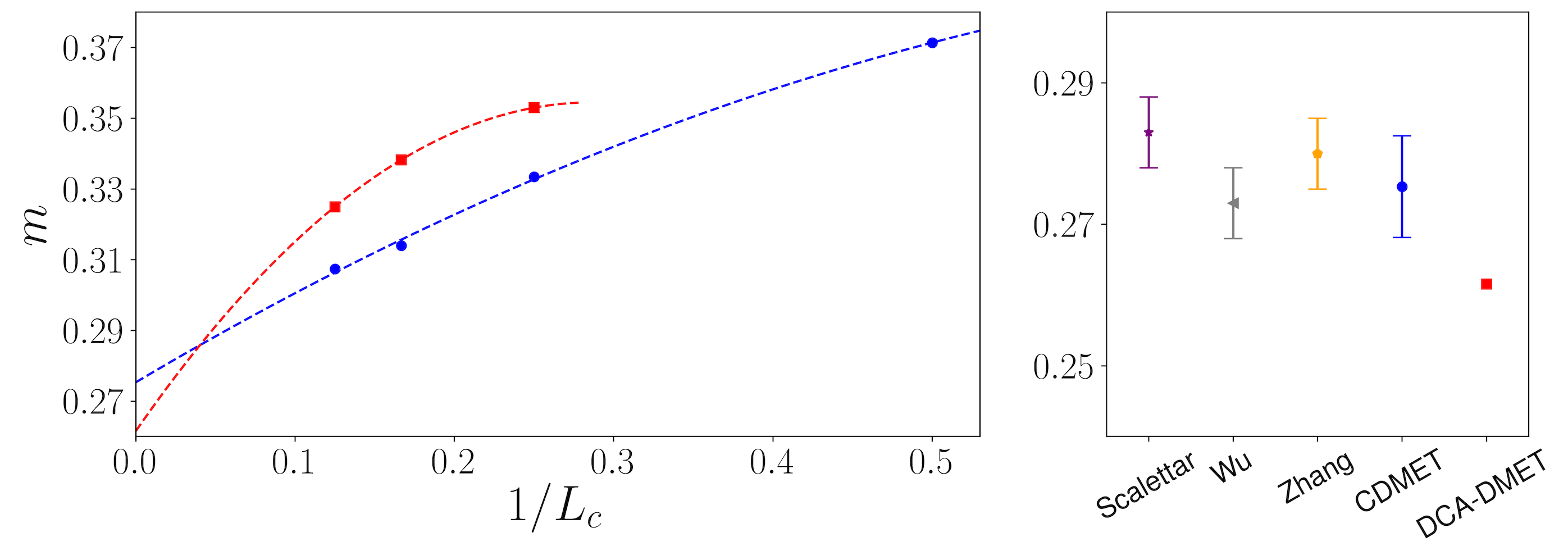
(c) U/t = 6

Figure 3.5: Left Panel: Antiferromagnetic order parameter $m$ versus $1/L_{c}$ in the 2D Hubbard model from CDMET (blue), DCA-DMET (red) and finite system AFQMC using TABC [1] (orange) and modified boundary conditions [3] (cyan).The DMET results extrapolate to the TDL uses the form $m(L)=a+bL_{c}^{-1}+cL_{c}^{-2}$. Right Panel: CDMET and DCA-DMET TDL estimates with error bars including fitting and AFQMC statistical uncertainties, compared to the determinantal Monte Carlo simulations by Scalettar and coworkers [5], pinning field QMC simulations by Wu and coworkers [6], AFQMC with TABC by Qin et. al. [1] and the modified boundary conditions by Sorella [3].

The TDL magnetic moment at $U/t=2$ is an example for which current literature estimates are in disagreement. While earlier AFQMC calculations in Refs. [5, 6, 2] appear to give an estimate close to $m\sim 0.09$, the AFQMC estimates from recent work of Sorella [3] and Qin et al [1] using larger clusters and modified and twist average boundary conditions predict a moment of $m\sim 0.120(5)$ and $0.119(4)$, respectively. This is much closer to our earlier DMET result of $m\sim 0.133(5)$ extrapolated from small clusters of up to $4\times 4$ in size. Revising this with the larger CDMET and DCA-DMET clusters in this work we can now confirm the larger value of the TDL magnetic moment, $m\sim 0.115(2)$ (CDMET) and $m\sim 0.120(2)$ (DCA-DMET) with very small error bars. The underestimate of the moment seen in earlier QMC work is likely due to the non-monotonic convergence of the moment with cluster size when using PBC, as identified in Sorella’s work [3]. In contrast to PBC calculations and the TABC calculations shown here (orange) which display some scatter, the dependence on fragment size is very mild once embedding is introduced. This once again highlights the ability of the embedded approach to capture some of the relevant aspects even of long-wavelength physics, leading to good convergence of local observables.

3.4 Conclusions

We carried out a detailed study of the fragment size convergence of density matrix embedding theory, using an auxiliary field quantum Monte Carlo solver (AFQMC) in order to large cluster sizes inaccessible from other impurity solvers. In addition to the cluster density matrix embedding formulation (CDMET), we study the “dynamical cluster” variant (DCA-DMET) that restores translational invariance in the fragment and accelerates finite size convergence. Using the half-filled one- and two-dimensional Hubbard models where AFQMC has no sign problem, as examples, we numerically explored the finite size convergence of the energy and the magnetization. The energy convergence of CDMET and DCA-DMET goes like $O(1/L_{c})$ and $O(1/L_{c}^{2})$ respectively, where $L_{c}$ is the linear dimension of the fragment, similar to that observed in cellular dynamical mean-field theory and the dynamical cluster approximation. The convergence of the magnetization follows a scaling relation related to the magnetic correlation function in CDMET, while the DCA-DMET converges more quickly than CDMET. In the case of the 2D Hubbard model, our thermodynamic limit extrapolations from both CDMET and DCA-DMET are competitive with the most accurate estimates in the literature, and in the case of $U/t=2$ where finite size effects are particularly strong, help to determine the previously uncertain magnetic moment.

In all the cases we studied in this chapter, the use of density matrix embedding, as compared to computations using bare clusters with any form of boundary condition, significantly decreased the computational cost required to obtain a given error in the TDL estimate, sometimes by orders of magnitudes. Since the computational scaling of the AFQMC solver employed here is quite modest with fragment size (cubic) this improvement would only be larger when using other, more expensive solvers.

The DCA-DMET formulation appears superior for large fragments due to the faster asymptotic convergence, however, it is typically less accurate for small fragments than CDMET. When performed in conjunction, the consistency of TDL estimates from CDMET and DCA-DMET serves as a strong check on the reliability of the DMET TDL extrapolations.

Chapter 4 Ground-State Phase Diagram of the Square Lattice Hubbard Model 

In this chapter, we present the ground-state phase diagram of the Hubbard and frustrated Hubbard models (with non-zero next-nearest-neighbor hopping) on the square lattice with density matrix embedding theory using clusters of up to 16 sites. We provide an error model to estimate the reliability of the computations and complexity of the physics at different points in the diagram. We find superconductivity in the ground-state as well as competition between inhomogeneous charge, spin, and pairing states at low doping. The estimated errors in the study are below $T_{c}$ in the cuprates and on the scale of contributions in real materials that are neglected in the Hubbard model.

In Sec. 4.1, we introduce the background of the study, focusing on the physics of the 2D Hubbard model. In Sec. 4.2, we present the detailed specifications of our DMET calculations and in a separate Section 4.3 we discuss the techniques to quantify the errors in the TDL estimates. We present the results and conclusions of our calculations in Sec. 4.4 and Sec. 4.5.

4.1 Introduction

The Hubbard model [134, 135, 136] is one of the simplest quantum lattice models of correlated electron materials. Its one-band realization on the square lattice plays a central role in understanding the essential physics of high temperature superconductivity [137, 61]. Rigorous, near exact results are available in certain limits [138]: at high temperatures from series expansions [139, 140, 141, 142], in infinite dimensions from converged dynamical mean-field theory [143, 44, 144, 145], and at weak coupling from perturbation theory [146] and renormalization group analysis [147, 148]. Further, at half-filling, the model has no fermion sign problem, and unbiased determinantal quantum Monte Carlo simulations can be converged [5]. Away from these limits, however, approximations are necessary. Many numerical methods have been applied to the model at both finite and zero temperature, including fixed-node, constrained-path, determinantal, and variational quantum Monte Carlo (QMC) [149, 150, 151, 152, 111, 153, 154, 155, 156, 157, 158], density matrix renormalization group (DMRG) [159, 160, 67], and dynamical cluster (DCA) [120, 121], (cluster) dynamical mean-field theories (CDMFT)  [161, 162], and variational cluster approximations (VCA) [163, 164]. (We refer to DCA/CDMFT/VCA collectively as Green’s function cluster theories). These pioneering works have revealed rich phenomenology in the phase diagram including metallic, antiferromagnetic, $d$-wave (and other kinds of) superconducting phases, a pseudogap regime, and inhomogeneous orders such as stripes, and charge, spin, and pair-density waves, as well as phase separation [138, 158, 149, 161, 150, 157, 67, 156, 153, 154, 165, 166, 167, 168, 169, 170, 171, 172, 173, 174, 175, 176, 70, 177, 178, 179, 180, 181, 182, 183]. However, as different numerical methods have yielded different pictures of the ground-state phase diagram, a quantitative picture of the ground-state phase diagram has yet to emerge.

It is the goal of this numerical study to produce such a quantitative picture as best as possible across the full Hubbard model phase diagram below $U/t=8$. We perform the calculations on the Hubbard model with the density matrix embedding theory (DMET), which is very accurate in this regime [54, 55, 184, 87, 185, 186, 85, 80], together with clusters of up to 16 sites and thermodynamic extrapolation. We carefully calibrate errors in our calculations, giving error bars to quantify the remaining uncertainty in our phase diagram. These error bars also serve, by proxy, to illustrate the complexity of the underlying physics for different Hubbard parameters. The accuracy we achieve is significantly higher than attained by earlier comparable Green’s function cluster calculations for the ground state. We also carefully estimate the finite size effects, which we find to have a crucial impact on the location of the phase boundaries of the antiferromagnetic and $d$-wave superconducting (SC) orders, in contrast to some early ground-state studies [167].

4.2 Methods

We study the one-band (frustrated) Hubbard model on the $L\times L$ square lattice

$$H=-t\sum_{\langle ij\rangle\sigma}a_{i\sigma}^{\dagger}a_{j\sigma}-t^{\prime}\sum_{\langle\langle ij\rangle\rangle\sigma}a_{i\sigma}^{\dagger}a_{j\sigma}+U\sum_{i}n_{i\alpha}n_{i\beta}$$ (4.1)

where $\langle\ldots\rangle$ and $\langle\langle\ldots\rangle\rangle$ denote nearest and next-nearest neighbors, respectively, $a_{i\sigma}^{(\dagger)}$ destroys (creates) a particle on site $i$ with spin $\sigma$, and $n_{i\sigma}=a_{i\sigma}^{\dagger}a_{i\sigma}$ is the number operator. The standard Hubbard model corresponds to $t^{\prime}=0$ (we fix $t=1$). We further study the frustrated model with $t^{\prime}=\pm 0.2$.

We use the broken particle-number symmetry, spin-unrestricted DMET formulation in this chapter. The basic principles of the method are outlined in Sec. 2.3, with detailed equations and algorithms presented in Appendix B.2. To obtain the ground-state phase diagram, we carry out DMET calculations using 2$\times$2, 4$\times$2, 8$\times 2$, and 4$\times$4 fragments, cut from a bulk square lattice with $L=72$. We considered $t^{\prime}=0,0.2,-0.2$, and $U=2,4,6,8$, and various densities between $n=0.6-1$. The impurity model ground-state $|\Psi\rangle$ is determined using a DMRG solver with a maximum number of renormalized states $M=2000$ (DMET self-consistency is performed up to $M=1200$), and which allows for $U(1)$ and $SU(2)$ spin symmetry breaking (see Sec. 2.4.2 and Appendix A.2). The energy per site $e$, local spin moment $m=\frac{1}{2}(n_{i\alpha}-n_{i\beta})$, double occupancy $D=\langle n_{i\alpha}n_{i\beta}\rangle$, and local $d$-wave pairing $d_{sc}=\frac{1}{\sqrt{2}}(\langle a_{i\alpha}a_{j\beta}\rangle+\langle a_{j\alpha}a_{i\beta}\rangle)$ were measured from the fragment part of $|\Psi\rangle$.

Local observables either are close to uniform in the entire fragment or exhibit tendencies to inhomogeneity. In the former case, we average the local observables in the central plaquette (so the average is consistent for all fragment sizes) and extrapolated to the thermodynamic limit (TDL) using a linear relationship with $N_{c}^{-1/2}$ as verified in Chapter 3. For the later case, reliable average and extrapolation are usually not possible, and we report these case as inhomogeneous order where a single order parameter cannot be extracted.

4.3 Error Estimation

The finite fragment DMET energies and measurements contain 3 sources of error relative to the exact TDL. These are from (i) errors in the DMET self-consistency, (ii) finite $M$ in the DMRG solver (This is only significant for the $8\times 2$ and $4\times 4$ clusters, corresponding to 32 fragment plus bath sites in the impurity model.),which also induces error in the correlation potential $u$, (iii) finite fragment size. The error from the use of a finite $72\times 72$ bulk lattice is so small as to not affect any of the significant digits presented here.

To estimate the TDL result, we (i) estimate DMET self-consistency quality by the convergence of expectation values in the last iterations, (ii) extrapolate DMRG energies and expectation values at finite $M$ to infinite $M$, using the linear relation with DMRG density matrix truncation error [187], (iii) estimate the error in $u$ due to finite $M$, by extrapolating expectation values from self-consistent $u(M)$ obtained with different solver accuracy, (iv) extrapolate fragment size to infinite size, with the $N_{c}^{-1/2}$ scaling appropriate to a non-translationally-invariant fragment (Sec. 2.5.3). Each of (i) to (iv) gives an estimate of an uncertainty component (for linear extrapolations, we use the 1$\sigma$ standard deviation), which we combine to obtain a single error bar on the DMET TDL estimates.

We use the energy per site as an example to discuss the error estimation in detail. The DMET self-consistency error is estimated as $\frac{1}{2}|e^{(n-1)}-e^{(n)}|$, where $e^{(n)}$ and $e^{(n-1)}$ are the energies per site of the last two DMET self-consistency iterations. A typical DMET calculation oscillates between two slightly different solutions with the magnitude of the oscillations decreasing with the number of iterations. We thus use the range of oscillation as a representation of the self-consistency error. The error distributions across the range of calculations in this chapter are shown in Fig. 4.1, with the average values on the side. For most points in the phase diagram, and for all fragment sizes, the self-consistency error is less than $0.0005t$. For $4\times 4$ fragments DMET calculations are the harder to converge, due to larger error in the impurity solvercalculations, giving a largest error of up to $0.002t$, and an average self-consistency error approximately twice as large as that for the other fragment shapes.

\begin{overpic}[width=281.85034pt]{conv_err} \put(100.0,37.0){ \begin{tabular}[]{ccc}\hline\cr\hline\cr{Shape}&{Mean} $\mathbf{(\times 10^{-4})}$&\\ \hline\cr 2$\times$2&2.2\\ 4$\times$2&1.8\\ 4$\times$4&3.7\\ 8$\times$2&2.0\\ \hline\cr\hline\cr\end{tabular} } \end{overpic}

Figure 4.1: Distribution and average value (side table) of the DMET self-consistency error in the energy per site (units of $t$) for each fragment shape.

For fragments larger than the $2\times$2 fragment (where our DMRG solver is not exact), there is the error due to using finite $M$ in the DMRG impurity solver. The error due to finite $M$ has two components:

1. variational error in the DMRG calculation, which is usually assumed proportional to the density matrix truncation error $\delta_{w}$,

2. the DMET correlation potential error $\delta_{u}$, as $\delta_{u}$ is a function of the impurity density matrices, and these have an error for finite $M$.

For the $4\times 2$ and $8\times 2$ fragments, the second source $\delta_{u}$ appears negligible. For these clusters, we carry out the DMET self-consistency with smaller $M$ to obtain the converged correlation potential $u$, then do a few DMRG calculations using large $M$ with fixed correlation potential $u$ to extrapolate to the $M\to\infty$ exact solver limit, thus obtaining the first error component due to the DMRG solver.

For $4\times 4$ fragments, the $U/t=2$ data is processed in this way as well. However, for other values of $U$ using the $4\times 4$ fragments, the DMRG truncation error can reach $10^{-3}$ for low to intermediate doping with computational tractable $M$, making the contribution from $\delta_{u}$ significant. To compensate for this, we first carry out the DMET self-consistency cycles with a series of different $M$’s up to 1200 , and linearly extrapolate the energy to the $M=\infty$ limit, $e_{1}$. This thus extrapolates errors from both source 1 and 2, assuming $\delta_{u}\propto\delta_{w}$. Another further set of DMRG calculations are done with $M$ up to 2000, using the converged correlation potential from the DMET self-consistency with the largest $M$. This second set of results are then extrapolated again against the truncated error to obtain an energy $e_{2}$, which only accounts for the error from source 1. Although the linear relation between the source 2 error and the truncation error need not hold in general, in practice, we find that $\delta_{u}=\frac{1}{2}|e_{1}-e_{2}|$ gives a reasonable estimate of $\delta_{u}$. Therefore, we report the $4\times 4$ fragment energy per site as $e_{4\times 4}=\frac{1}{2}(e_{1}+e_{2})$, with a final uncertainty of

$$\delta e_{4\times 4}^{2}=\delta_{u}^{2}+\delta e_{1}^{2}+\delta e_{2}^{2}$$ (4.2)

where $\delta e_{1}$ is a combination of the linear regression uncertainty and the uncertainties of the original data points (from DMET self-consistency error), while $e_{2}$ does not have any self-consistency error. Fig. 4.2 illustrates the set of computations and linear extrapolations performed with each $4\times 4$ cluster to obtain the $4\times 4$ cluster energy and error estimate.

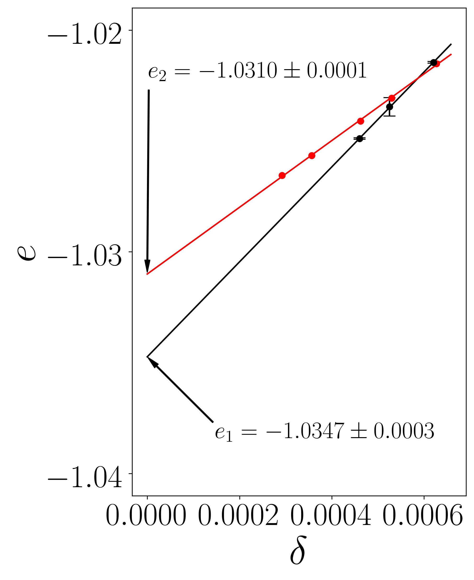
(a) $U/t=4$ $e=-1.033(2)$

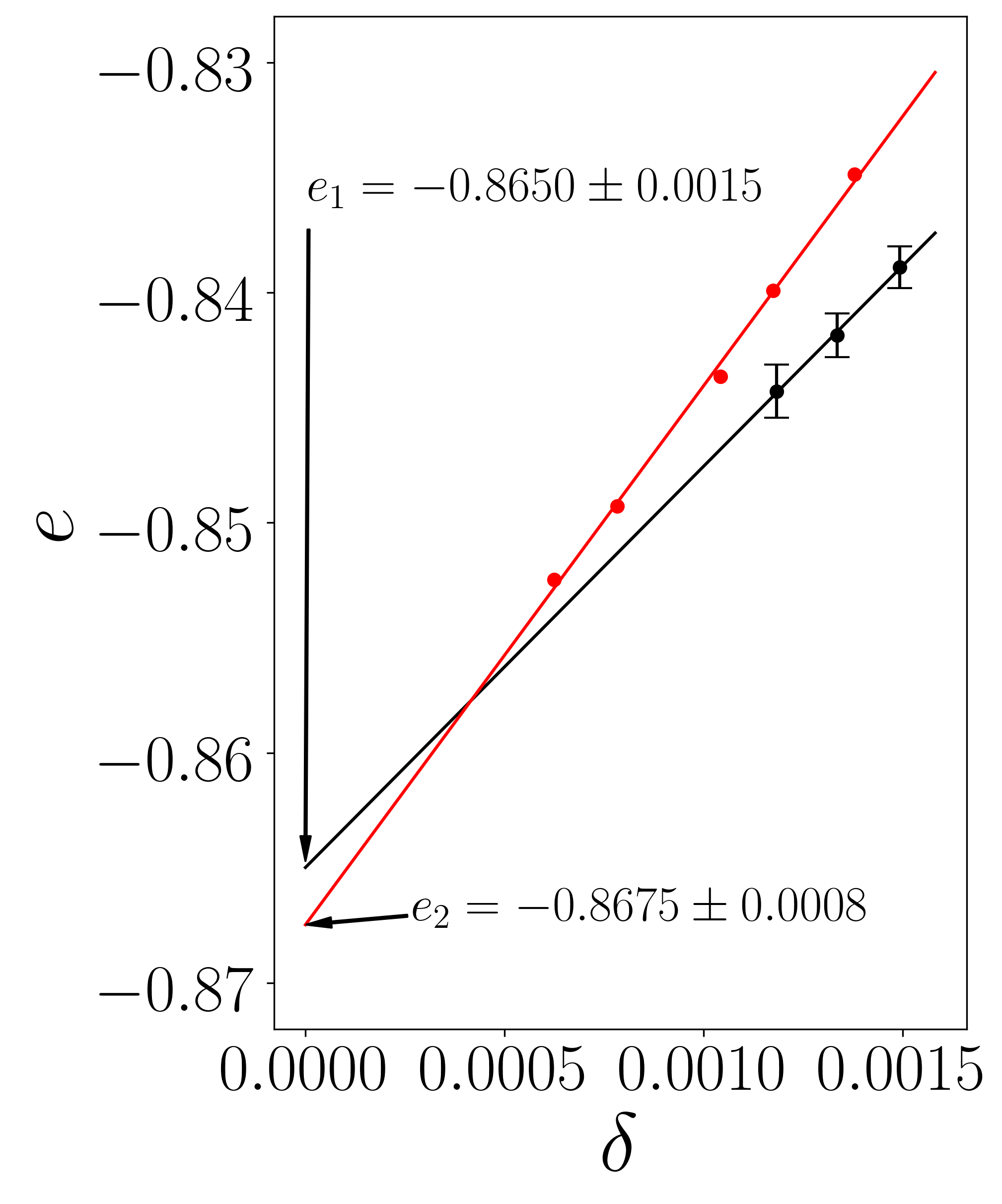
(b) $U/t=6$ $e=-0.866(2)$

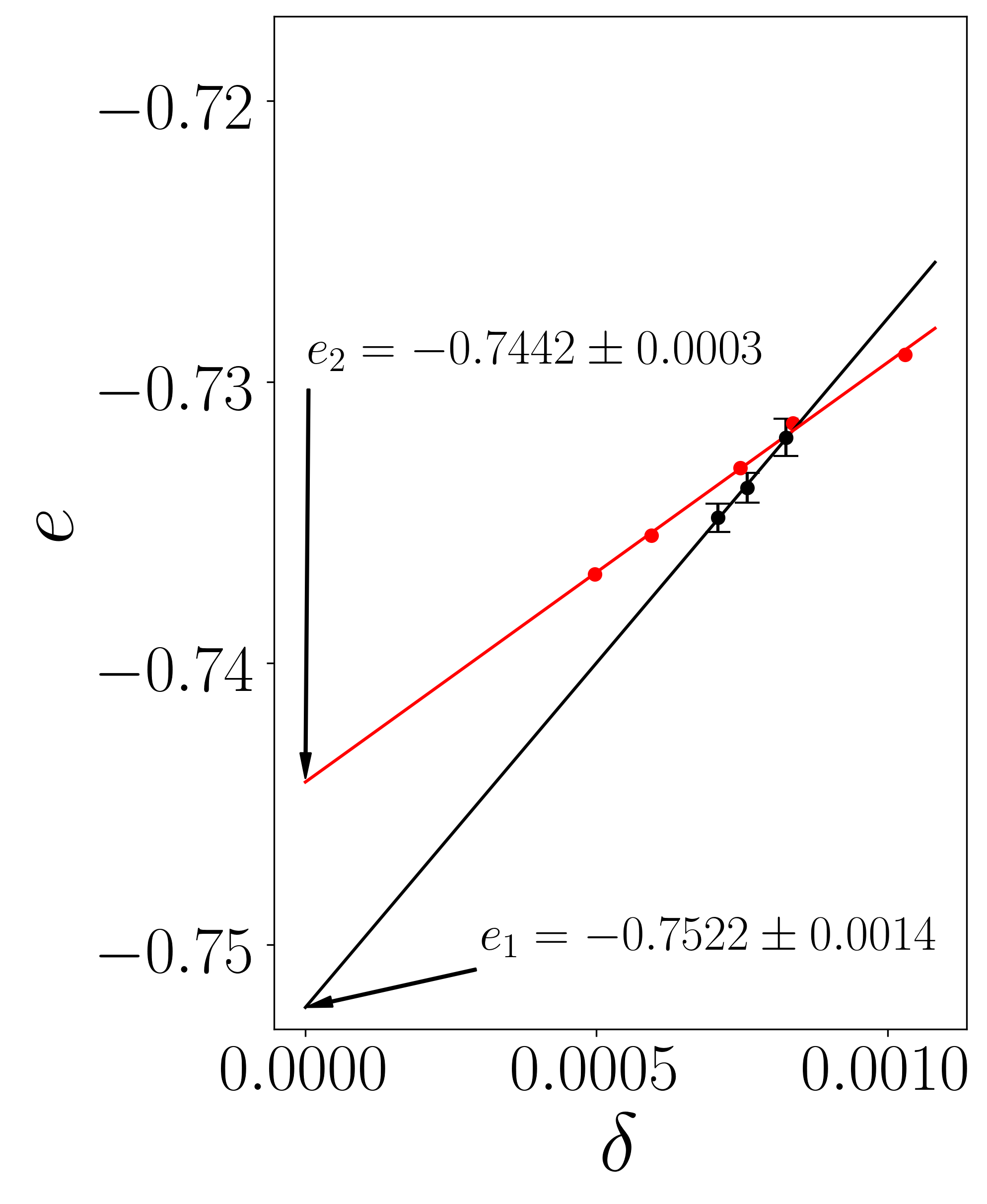
(c) $U/t=8$ $e=-0.748(4)$

Figure 4.2: Estimation of the DMRG $M=\infty$ energy per site and the associated error bars due to finite $M$, for $4\times 4$ fragments. (See the text for detail.) The plots are shown for $t^{\prime}=0,n=0.875$.

After obtaining the energy per site and other observables for each fragment size, we extrapolate to the TDL using the relation $\Delta e_{N_{c}}\propto N_{c}^{-1/2}$. Since both the $4\times 4$ and $2\times 8$ fragments are of 16 sites, we must choose which one to use in the extrapolation. We believe that the $4\times 4$ fragments have less finite size error than the $8\times 2$ fragments, and thus we generally use these in the extrapolation. However, at certain points in the phase diagram (e.g. at strong coupling, or negative $t^{\prime}$) there is a strong tendency towards inhomogeneity, and the new order the new order the $4\times 4$ fragments, resulting in a much higher energy than for the $8\times 2$ fragments. In such cases, namely, when (a) the $4\times 4$ and $8\times 2$ fragments show different orders, and (b) the $8\times 2$ cluster is lower in energy, we use the $8\times 2$ cluster energy for the extrapolation.

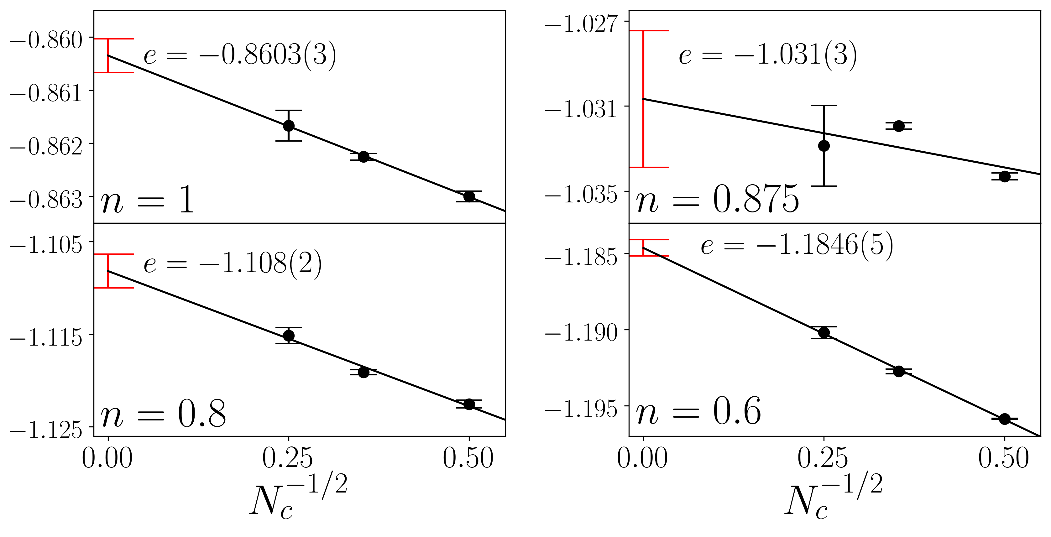
Figure 4.3: Fragment size extrapolation of the energies per site for $U=4,t^{\prime}=0$ at various fillings. The black dots are finite size results. The red error bars are the confidence intervals for the TDL estimates.

The fragment size extrapolation works considerably well given the limited number of data points and small sizes of the clusters, although it contributes the main source of error in the uncertainty of TDL estimates. In Fig. 4.3 we show examples of the finite size extrapolation at $U/t=4$. The error bars shown for TDL estimates include both the error from the linear extrapolation and the propagated uncertainties from the finite fragment calculations. At half-filling and in the overdoped region ($n<0.8$), the linear relation appears quite good even with these small clusters. In the underdoped region, however, the energy per site is more strongly dependent on the cluster shape, often because the system has a strong tendency to establish an inhomogeneous phase (see Sec. 4.4 for detail). Nontheless, even in the underdoped region, the error model appears to give a reliable estimate of the energy per site at the TDL, albeit with a large uncertainty.

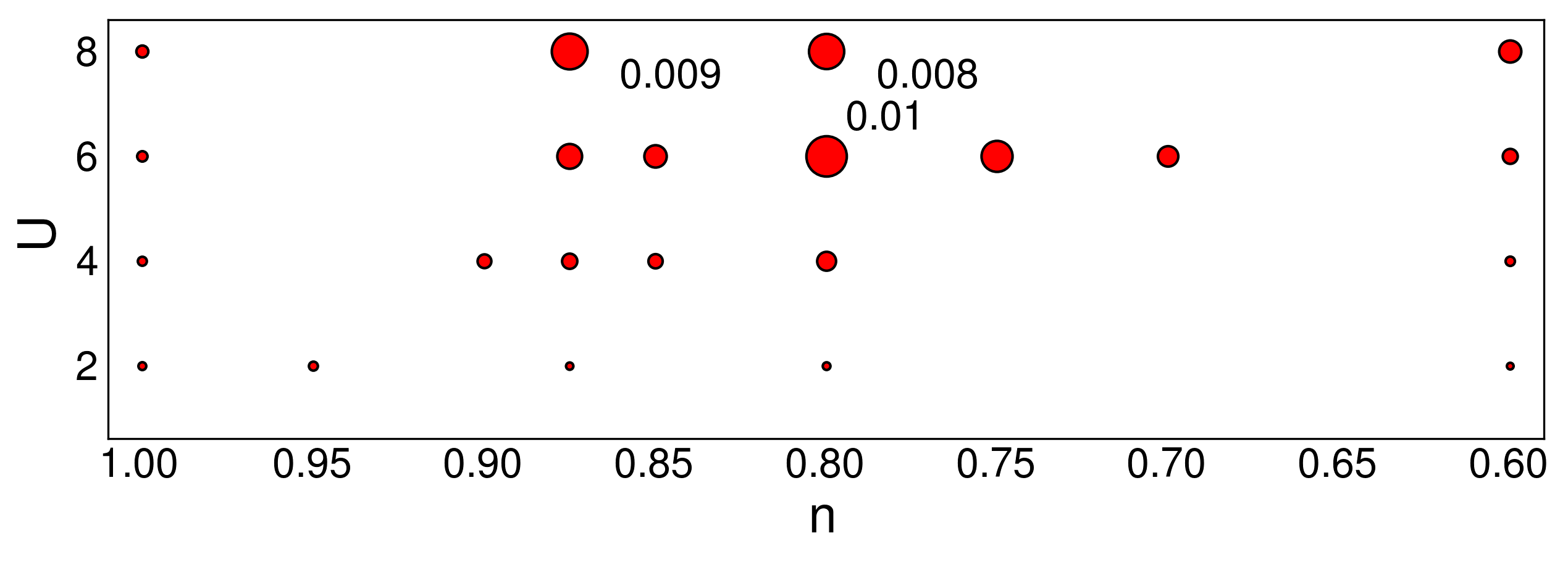
(a) $t^{\prime}=0.2$

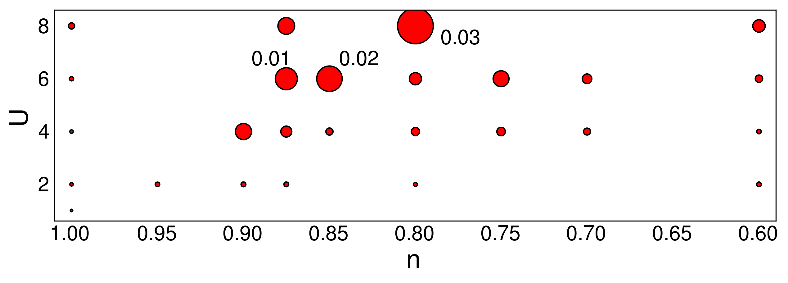
(b) $t^{\prime}=0$

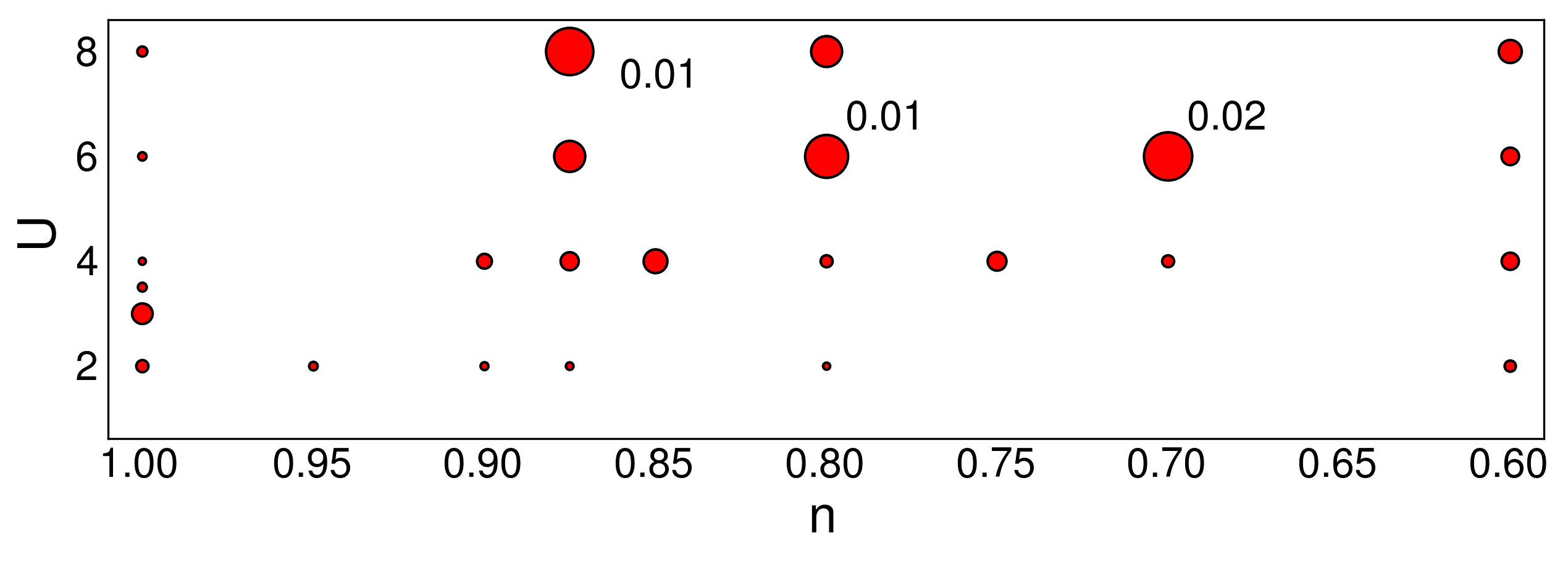
(c) $t^{\prime}=-0.2$

Figure 4.4: Numerical uncertainty map of DMET energies per site for the (frustrated) Hubbard model with $t^{\prime}=0.2,0$ and $-0.2$. The areas of the circles are proportional to the estimated uncertainties.

Fig. 4.4 shows the uncertainties of the energy per site TDL estimates for all the points in our calculations. As one would normally expect, the accuracy away from half filling is significantly lower than at half filling, with the largest errors found in the underdoped region of $n=0.8\sim 0.9$, where the solution is sensitive to cluster shapes because of phase boundaries and/or the onset of competing inhomogeneous orders, thus introducing the largest errors from fragment size extrapolation. We also see from the Fig. 4.4 that the maximum uncertainty for $t^{\prime}=0.2$ is smaller than that for $t^{\prime}=0$ and $t^{\prime}=-0.2$ ($0.01t$ versus $0.03t$ and $0.02t$, respectively), implying the completing order effect is weaker for positive $t^{\prime}$ than in the zero or negative $t^{\prime}$ case.

We discussed energies per site in this section as an example. The order parameters are extrapolated to the TDL and the uncertainties associated with them are estimated, following the same procedure. Whenever necessary, we use the $Z$-score (estimated value divided by its standard deviation) to describe the robustness of the order.

4.4 Results

The quantitative analysis of the sources of error gives us confidence to distinguish the physics from artifacts in the orders we see from DMET calculations. We now look at the calculation results and try to interpret them, with the map of uncertainties (Fig. 4.4) in mind.

In Sec. 4.4.1, we present the phase diagram using our TDL estimates of the all the parameter sets. In the subsequent sections we analyze the results of different regions of the phase diagram in greater detail.

4.4.1 Overview

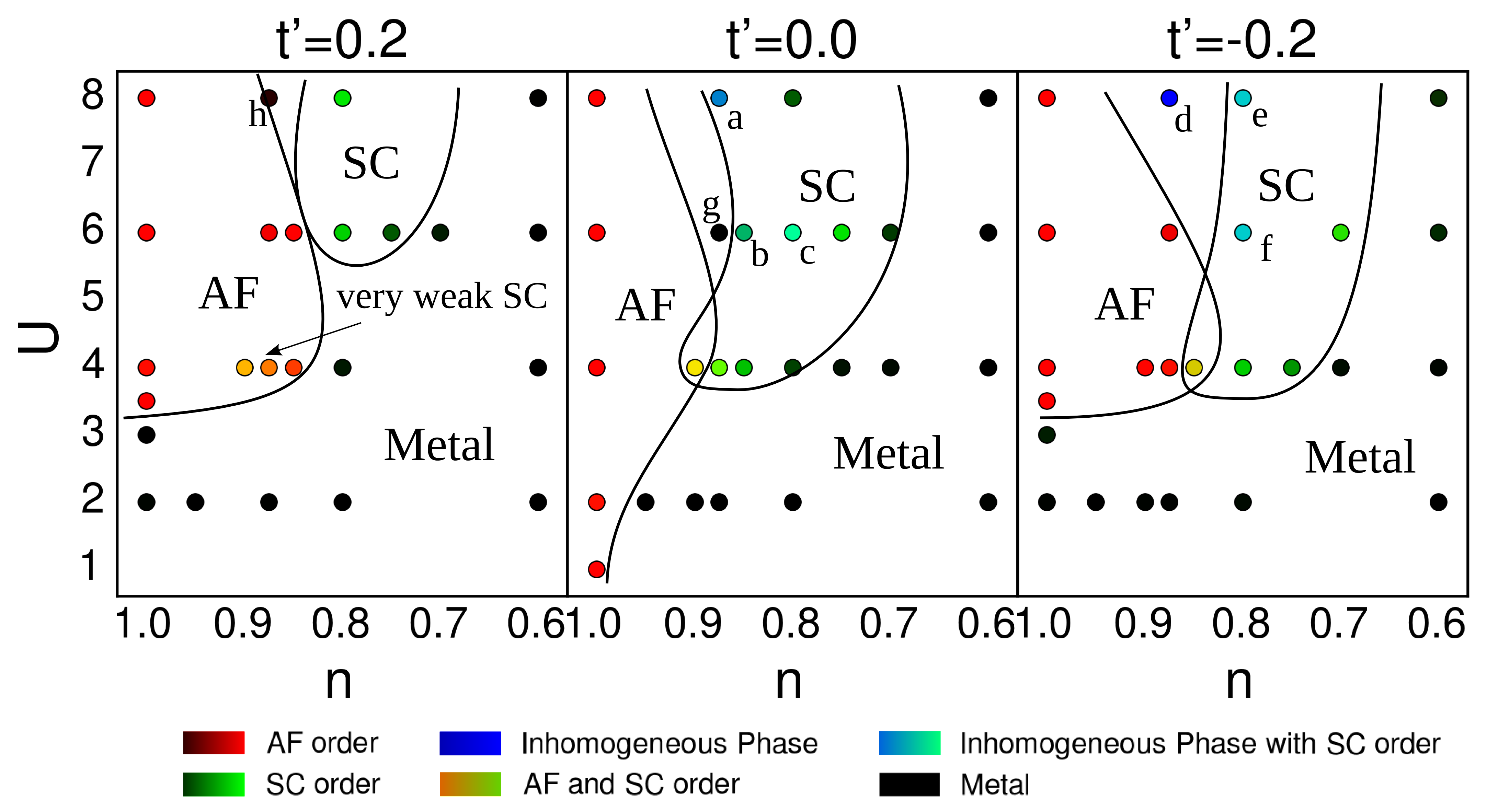
Figure 4.5: Phase diagrams of the standard and frustrated Hubbard models. Orders are represented with three primary colors: red (antiferromagnetism), green ($d$-wave superconductivity) and blue (inhomogeneity), with the brightness proportional to the robustness of the order. The points highlighted with letters: (a) local phase separation; (b) $d$-wave SC with a slight modulation in $(\pi,\pi)$ direction; (c) SC with a weak spin density wave (SDW); (d) a “classic” stripe phase; (e) stripe with pair-density wave (PDW) coexisting with SC; (f) CDW and spin $\pi$-phase shift; (g) and (h) intermediate points between AF and SC where both order parameters extrapolate to zero. Phase boundaries are guides only.

We present the DMET phase diagrams in Fig. 4.5. Interestingly, they feature many behaviors previously proposed in different studies. In particular, we observe (i) an antiferromagnetic (AF) phase at half-filling; (ii) a metallic phase at large dopings and at small $U$, enhanced by frustration; (iii) a region of $d$-wave superconducting (SC) order at intermediate dopings and sufficiently large $U$; (iv) a region of coexisting AF and SC order; (v) a region rich with inhomogeneous charge, spin, and superconducting orders that are very sensitive to the Hubbard parameters; (vi) points in between the AF and SC phase where the AF and SC orders extrapolate to zero. (The metallic phase is predicted to be unstable at weak coupling and large dopings from weak coupling expansions [188, 148], but the relevant parameter region is outside the scope of this study.) At $t^{\prime}=0$,for $U/t=8,n=0.875$,an SC state with strong inhomogeneity appears which creates large uncertainties in the extrapolated order parameters; thus, the precise location of the SC phase boundary at $U/t=8$ is uncertain. Overall, the existence of all the phases and their boundaries are consistent with the general understandings of the 2D Hubbard model.

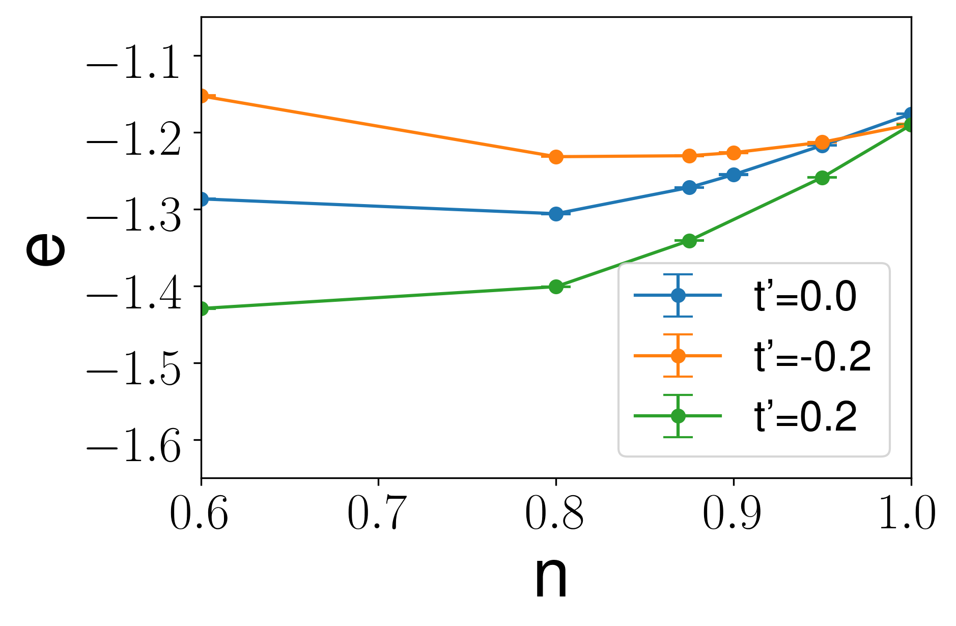
(a) $U/t=2$

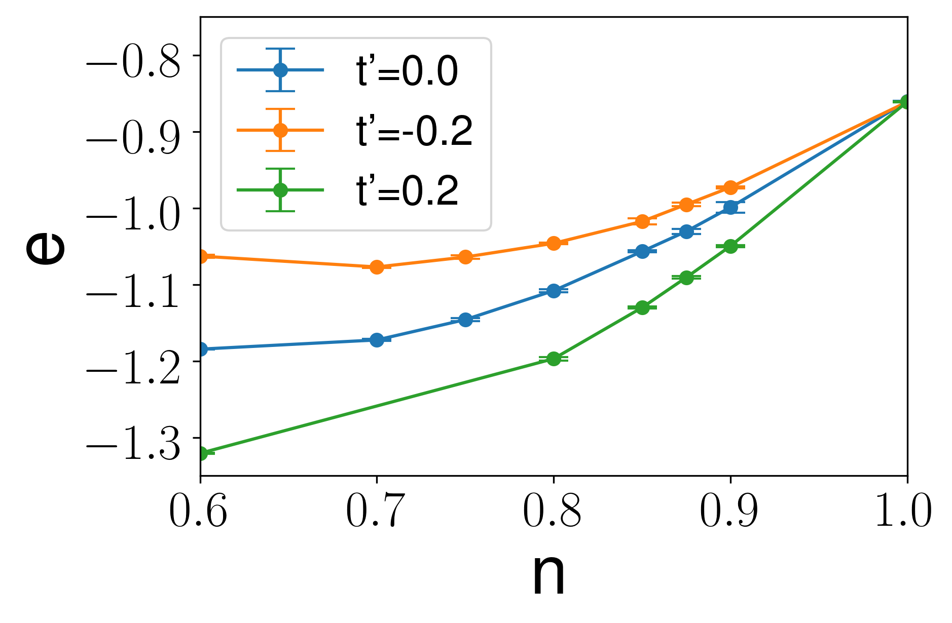
(b) $U/t=4$

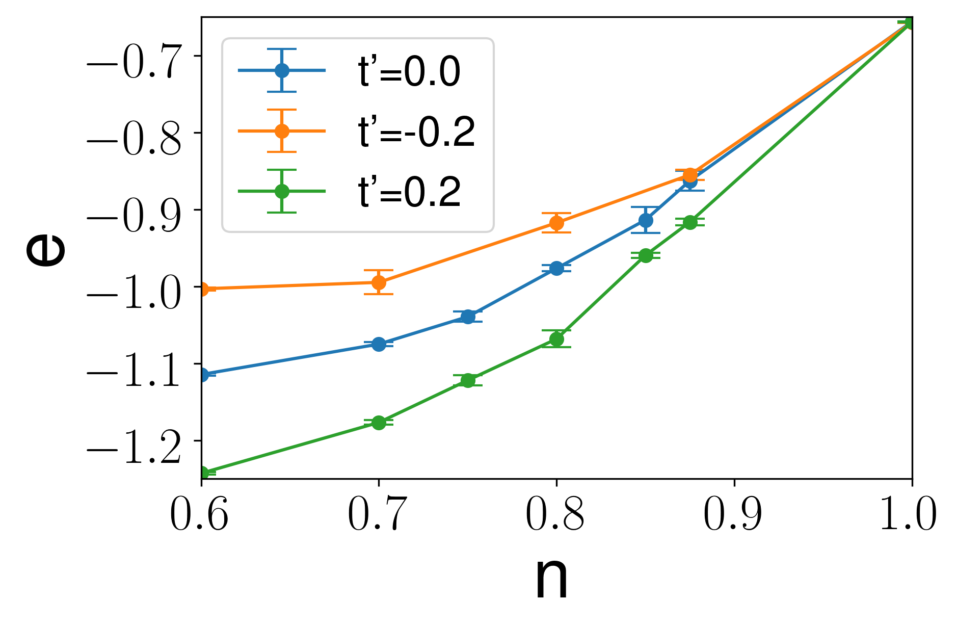
(c) $U/t=6$

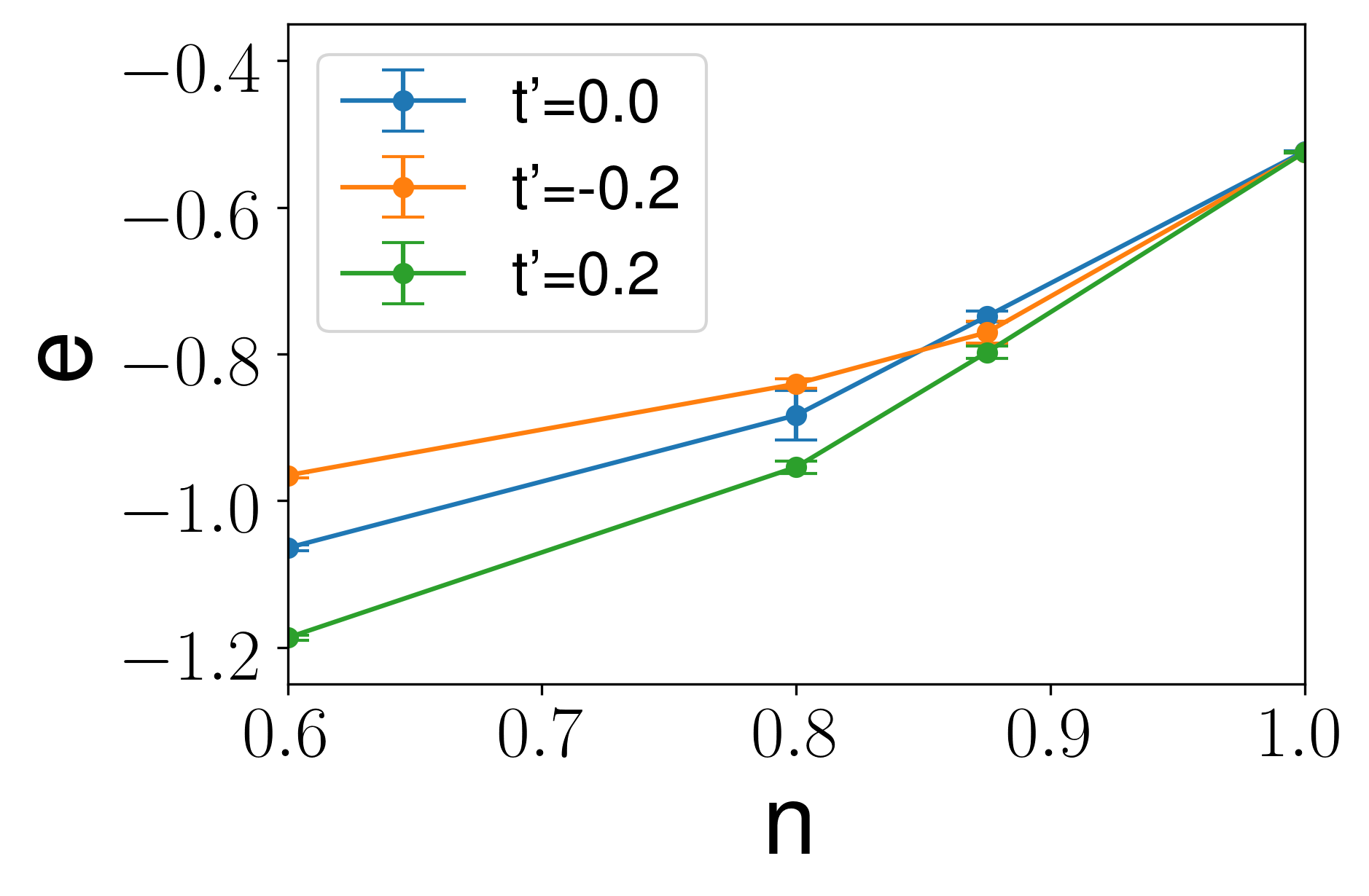
(d) $U/t=8$

Figure 4.6: DMET estimates of the 2D Hubbard model energies per site in the TDL.

In Fig. 4.6, we show the estimated TDL energies across the parameter space. At half-filling, the energy in the frustrated models $t^{\prime}=\pm 0.2$ are slight below those in the standard Hubbard model, due to the kinetic energy relaxation. The effect is smaller for larger $U$ where the electrons are more confined. At large doping, e.g., $n\leq 0.8$, the energy order is dominated by the kinetic effects, i.e. $e_{t^{\prime}=-0.2}>e_{t^{\prime}=0}>e_{t^{\prime}=0.2}$. The energy curves show more complicated behavior in the underdoped region, especially at large $U$ and for $t^{\prime}=0$ and $-0.2$, indicating complicated behaviors in this region, as we will discuss later.

4.4.2 Half-Filling Results

We now look at the results for the half-filled case in detail. In Table 4.1 and Fig. 4.7 we compare the DMET energies per site, double occupancies, and staggered magnetizations with exact estimates at half-filling, as obtained from auxiliary field quantum Monte Carlo (AFQMC) extrapolated to infinite size  [1], and DMRG on long open cylinders, extrapolated to infinite width and length [2]. For comparison, we also show recent DCA energies computed at the lowest published temperatures, $T=0.05-0.15$t [7].

Table 4.1: Ground-state energy per site of the half-filled ($t^{\prime}=0$) 2D Hubbard model. All the numbers are extrapolated to the TDL. AFQMC and DMRG results are from Refs. [1, 2].

$\mathbf{U/t}$	DMET	AFQMC	DMRG
2	-1.1764(3)	-1.1763(2)	-1.176(2)
4	-0.8604(3)	-0.8603(2)	-0.862(2)
6	-0.6561(5)	-0.6568(3)	-0.658(1)
8	-0.5234(10)	-0.5247(2)	-0.5248(2)
12	-0.3686(10)	-0.3693(2)	-0.3696(3)

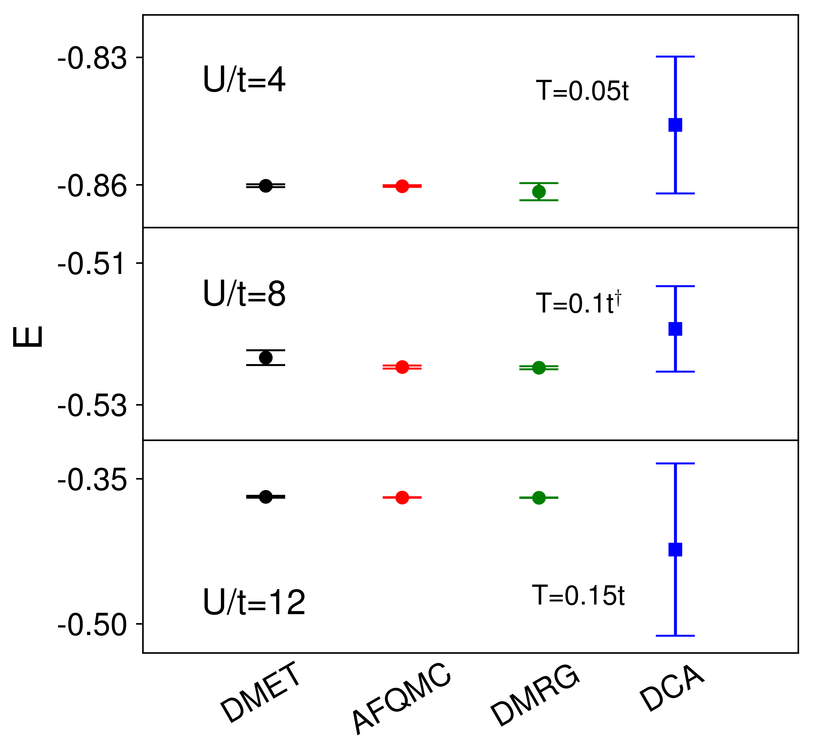
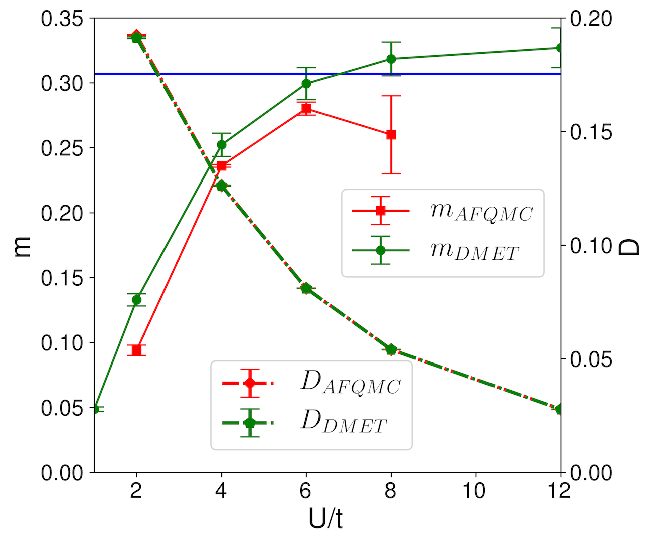
Figure 4.7: Results for the half-filled ($t^{\prime}=0$) Hubbard model. (a) Energy per site. Ground state estimates from DMET, AFQMC and DMRG, compared to a recent DCA study [7]. The temperatures are the lowest published values in the DCA study. ^(†) DCA data at $U/t$=8 is from 50-site cluster calculations, and not extrapolated to the TDL. (b) Staggered magnetization ($m$) and double occupancy($D$) at half-filling. The blue line is the spin-$\frac{1}{2}$ Heisenberg limit $m=0.3070(3)$ [8].

The data shows the high accuracy of the DMET energies at half filling. The error bars from DMET, AFQMC, and DMRG are all consistent, with an accuracy better than 0.001$t$. Indeed, the DMET error bars are competitive with the exact “statistical” error bars of AFQMC up to $U/t=6$. As a point of reference, the DMET uncertainty is one to two orders of magnitude smaller than finite temperature contributions to recent low-temperature benchmark DCA calculations (Fig. 4.7), and is similarly two to three orders of magnitude smaller than energy errors in earlier zero-temperature Green’s function cluster calculations [189].

Fig. 4.7 further gives the half-filling staggered magnetizations and double occupancies computed with DMET as compared with AFQMC. The DMET double occupancies are obtained with similar error bars to the AFQMC estimates, suggesting the good agreement of the total energy is not from an effect of error cancellation. The staggered magnetization exhibits larger discrepancies at the smallest $U/t=2$, but with later revised AFQMC estimates $m\sim 0.12$ the agreement is excellent [1]. For $U/t\geq 4$, DMET gives similar, or in fact more accurate staggered magnetization than AFQMC. At our largest available $U/t=12$, we find $m=0.327(15)$, slightly above the exact Heisenberg value $m=0.3070(3)$  [8] (corresponding to $U/t=\infty$ limit).

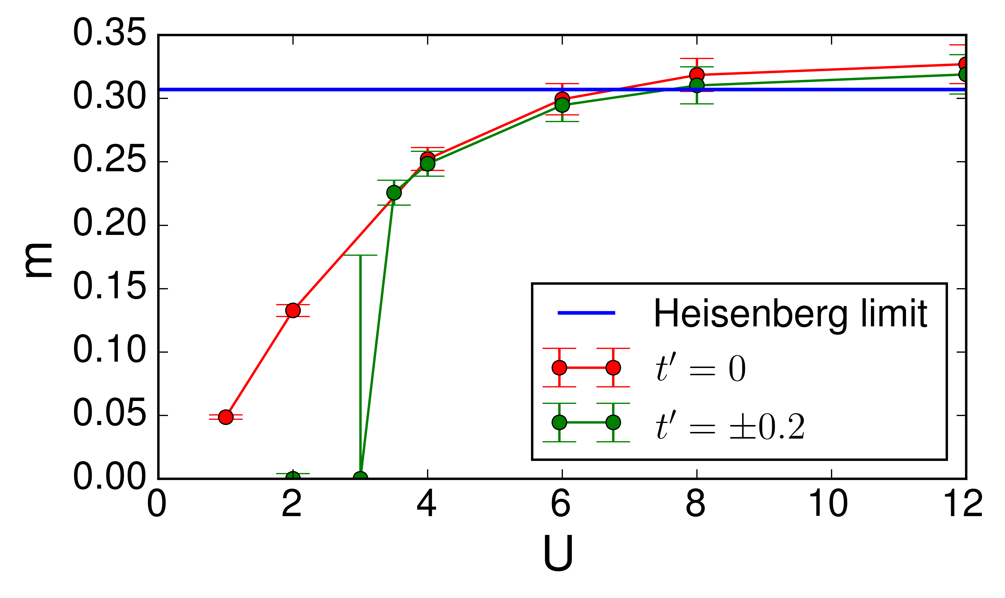
Figure 4.8: Staggered magnetization ($m$) of the half-filled Hubbard model for $t^{\prime}=\pm 0.2$, compared to $t^{\prime}=0$.

The staggered magnetization for the frustrated Hubbard models at half filling (compared to the $t^{\prime}=0$ standard Hubbard model and the Heisenberg limit) are shown in Fig. 4.8. Because of the particle-hole parity, the magnetization curve is identical for $t^{\prime}=\pm 0.2$. The onset of antiferromagnetism is at finite $U$ in the frustrated model, somewhere between $U/t=2$ and $3.5$. This is consistent with previous quantum Monte Carlo simulations [190].

The large error bar at $U/t=3$ reflects the increasing quantum fluctuations near the phase boundary, leading to multiple possible solutions in self-consistent embedding methods. The results are thus sensitive to initial conditions and fragment shape, etc., resulting in a huge uncertainty in the TDL results.

4.4.3 Doped Hubbard Model in Weak to Moderate Coupling

The impressing accuracy of half-filling results lend confidence to the DMET TDL estimates of the energy per site and observables and their associated error bars. The same procedure is used to compute the quantities and error bars for the doped Hubbard model.

Table 4.2: Ground-state energy per site of the ($t^{\prime}=0$) 2D Hubbard model at $U/t=4$. All the numbers are extrapolated to the TDL. CP-AFQMC and DMRG results are from Refs. [1, 2].

$\mathbf{n}$	DMET	CP-AFQMC	DMRG
0.875	-1.031(3)	-1.026(1)	-1.028(2)
0.8	-1.108(2)	-1.110(3)	-1.1040(14)
0.6	-1.1846(5)	-1.185(1)	-
0.3	-0.8800(3)	-0.879(1)	-

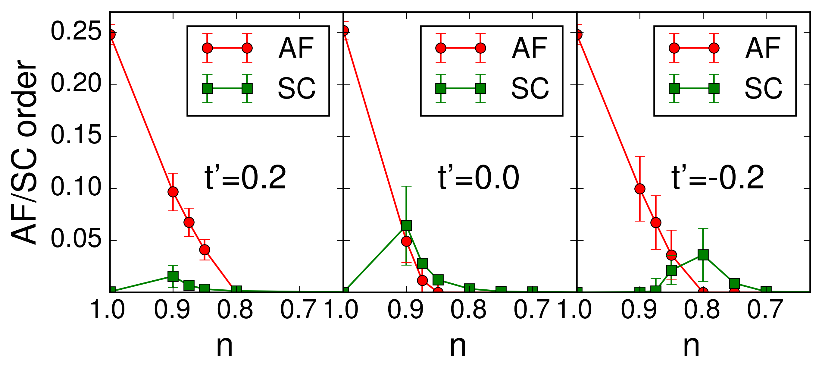
Figure 4.9: Antiferromagnetic (red circle) and ($d$-wave) superconducting (green square) order parameters for the (frustrated) 2D Hubbard models at $U/t=4$.

We start with $U/t=4$. For benchmark purpose, we compare the energies per site from DMET, DMRG and the constrained path (CP) AFQMC, a sign-free QMC with a bias that disappears at low density and small $U$ [111, 153] in Table. 4.2. For $n\leq 0.6$, a parameter regime where CP-AFQMC is very accurate, the DMET and CP-AFQMC energies agree to $0.001t$, while the error bars from DMET, CP-AFQMC and DMRG are comparable in the underdoped region.

Fig. 4.9 shows the averaged (over the central plaquette) AF and $d$-wave SC order parameters as a function of filling for $U/t=4$. As expected, the SC order lives at the proximity of the AF order and is a small effect compared to the magnetization. We find that for $t^{\prime}=0$, the peak in SC order is around $\langle n\rangle=0.9$ and SC extends to $\langle n\rangle\sim$0.8. The figures also show that next-nearest-neighbor hopping $t^{\prime}=0.2$ stabilizes AF versus SC, and the reverse is true for $t^{\prime}=-0.2$. The suppression (enhancement) of SC order with positive (negative) $t^{\prime}$ is consistent with the stronger superconductivity found in hole-doped materials [191, 192, 193].

The presence of SC in the Hubbard model ground-state has previously been much discussed. The strongest SC order found in DMET roughly occurs in the same region as seen in earlier Green’s function cluster calculations [167, 173]. However, this region is not typically found to be superconducting in ground-state wavefunction calculations using DMRG and AFQMC on finite lattices, even though such calculations achieve significantly higher energy accuracies than the Green’s function cluster studies  [154, 67, 194, 2]. The significance of the DMET result is that the energy error bar in this region (e.g., $0.001t$ per site for $U/t=4,n=0.8,t^{\prime}=−0.2$) is comparable to or better than the accurate ground-state wavefunction calculations, yet SC order is still seen. This strongly suggests that SC is, in fact, the ground-state order.

Table 4.3: Energies per site for various 16-site fragments at $U/t=4$.

$\mathbf{t^{\prime}}$	$\mathbf{n}$	$\mathbf{e_{8\times 2}}$	$\mathbf{e_{4\times 4}}$
0.2	0.8	-1.2036(2)	-1.204(2)
	0.875	-1.0944(1)	-1.095(1)
0	0.8	-1.1164(2)	-1.1151(8)
	0.875	-1.0284(1)∗	-1.033(2)
-0.2	0.8	-1.10483(6)∗	-1.0507(4)
	0.85	-1.0162(1)∗	-1.020(2)
	0.875	-0.9966(1)∗	-0.9989(7)

^∗ These $8\times 2$ fragment results show significant inhomogeneity.

Even at moderate $U/t=4$, there is already tendency towards inhomogeneity. The $8\times 2$ fragment calculations result in an inhomogeneous state at dopings $n=0.8$ to $0.875$, although the energies are significantly higher than obtained with the $4\times 4$ fragments at the same fillings. In Fig. 4.10(b) and  4.10(c), we show two such examples with spin and pairing modulation. As a comparison, we show the $t^{\prime}=0.2$ result (Fig. 4.10(a)) with the same doping to verify that this is not an artifact. Table 4.3 further shows the energies per site in the underdoped region at $U/t=4$. All the $4\times 4$ fragment calculations are homogeneous, while some of the $8\times 2$ calculations give an inhomogeneous solution, at a higher energy, suggesting that the ground state at $U=4$ is homogeneous, or inhomogeneous with a very long wavelength that does not fit in our cluster shapes.

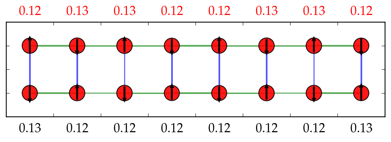
(a) $t^{\prime}=0.2$

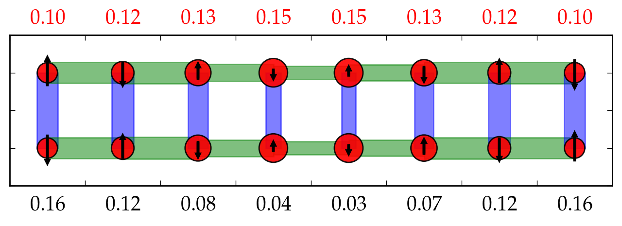
(b) $t^{\prime}=0$

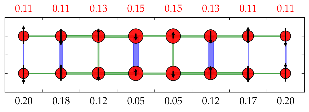
(c) $t^{\prime}=-0.2$

Figure 4.10: Charge, spin and pairing orders for the $8\times 2$ fragment calculations at $U/t=4,n=0.875$.

We then briefly discuss results at weak coupling $U/t=2$. We find the antiferromagnetism (in the standard Hubbard model) is destroyed already at small doping $x=0.05$ away from half-filling. (For the frustrated Hubbard model there is no AF order even at half-filling) While the extrapolated AF order is zero, the uncertainty $\delta m$ is still large ($\sim 0.05$ at $x=0.05$), reflecting short-range AF fluctuations still exist. $\delta m$ decays exponentially as we increase doping. At $U/t=2$ we do not find $d$-wave superconductivity to within in numerical precision.

4.4.4 Doped Hubbard Model in Stronger Coupling

The stronger coupling region of the 2D Hubbard model has a more direct connection with the cuprate physics. We are most interested in the underdoped region between the AF and the SC phases. In this region, a variety of spin-density  [195, 169, 175, 154, 196, 197, 169, 171, 172, 175], charge-density [198, 199, 200, 154], pair-density wave [72, 200, 76, 201], and stripe orders [202, 203, 159, 67, 204, 205, 197, 70, 177], have been posited in both the Hubbard model and the simpler $t$-$J$ model. These inhomogeneous phases are proposed to be relevant in the pseudogap physics  [69, 71, 72, 74, 73, 75, 76]. Recent infinite projected entangled pair state (iPEPS) studies of the $t$-$J$ model and Hubbard model at large $U/t=8$ suggest that inhomogeneous and homogeneous states are near degenerate at low doping and can be stabilized with small changes in the model parameters [205, 4].

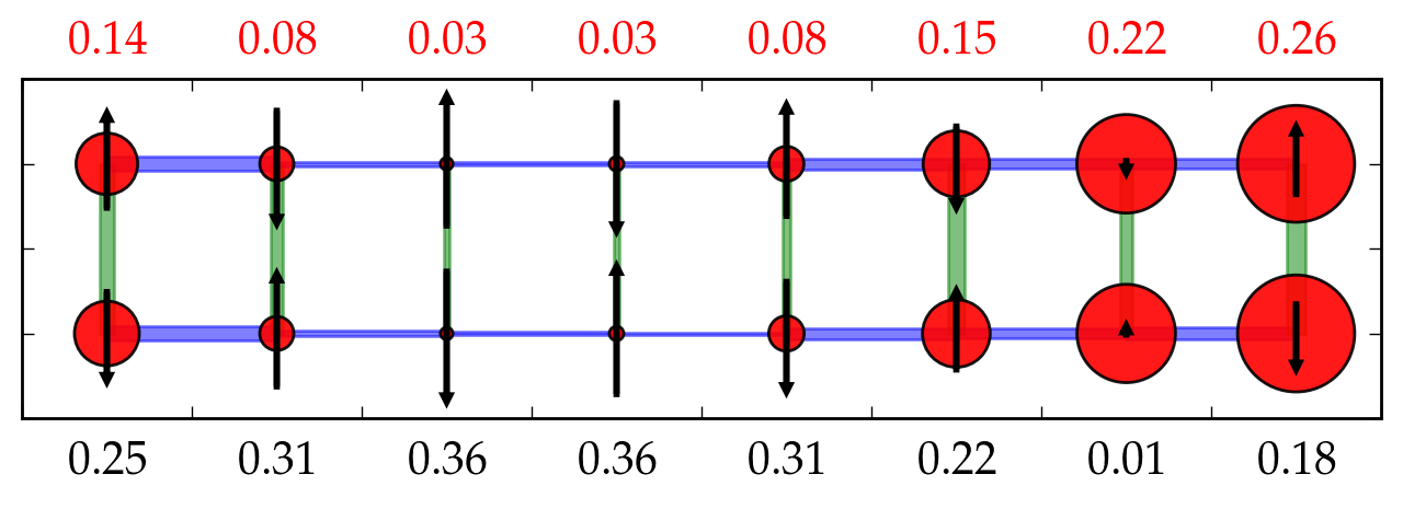
(a) $n=0.875$ $t^{\prime}=0$

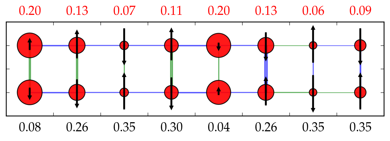
(b) $n=0.875$ $t^{\prime}=-0.2$

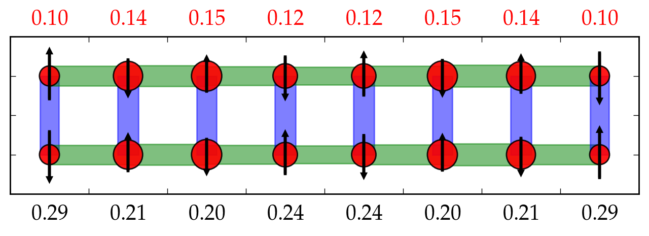
(c) $n=0.875$ $t^{\prime}=0.2$

Figure 4.11: Local charge, spin and pairing orders in the (frustrated) Hubbard model at various points in the strong coupling regime ($U/t$=8).

Our work indicates similar behavior in the Hubbard model. For large $U$ and low doping $n=0.875-0.8$ we find many points with inhomogeneous orders. Interestingly, the kinds of inhomogeneity we observe are extremely rich, and some representative examples are shown in Fig. 4.11. These correspond to (i) a local phase separation between a half- filled, antiferromagnetic phase and a superconducting ribbon [Fig. 4.11(a)]; (ii) a classic stripe phase order [Fig. 4.12(c)] very similar to that seen in earlier DMRG ladder studies [67] (there is also a coexisting weak PDW, exhibiting a sign change across the cell, consistent with earlier stripe proposals [201]); (iii) inhomogeneities in the pairing order coexisting with the charge and spin orders in, e.g., Fig. 4.11(c), similar to a recent theoretical proposal (see, e.g., Ref. [76]). Fig. 4.11(c) shows an example at 1/8 doping with positive $t^{\prime}$, where the inhomogeneity is much weaker. Again the next-nearest-neighbor hopping $t^{\prime}$ plays an important role in stablishing or destroying the inhomogeneous orders, providing an explanation for the particle-hole asymmetry in cuprates.

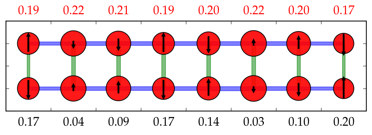
(a) $U/t=4$ $e_{\text{diff}}=0.002$

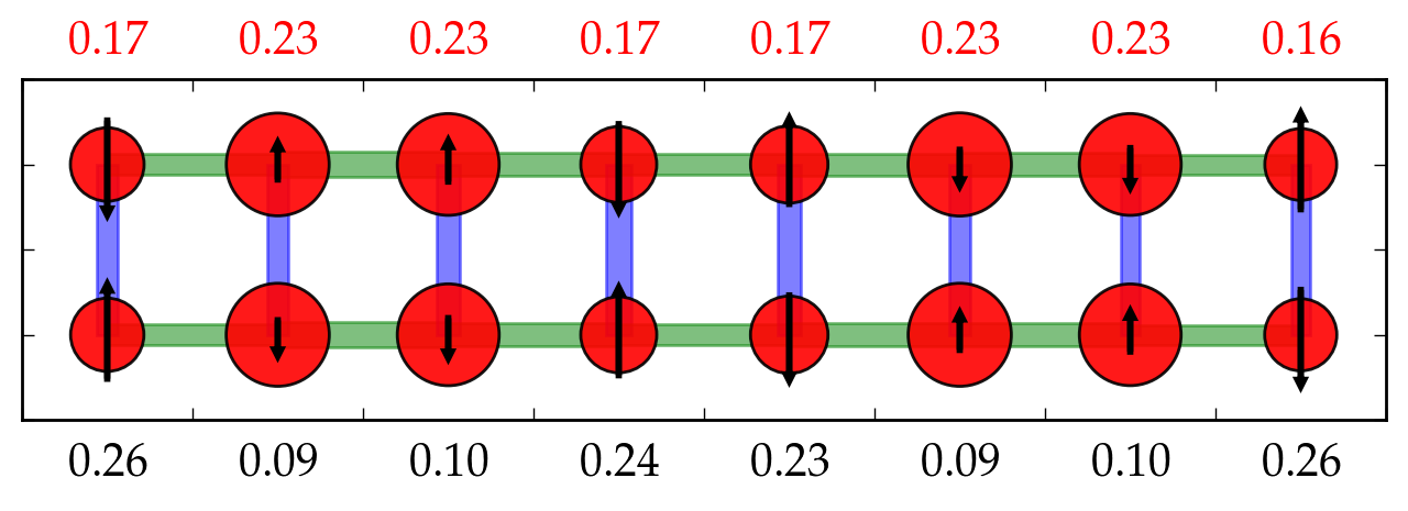
(b) $U/t=6$ $e_{\text{diff}}=-0.001$

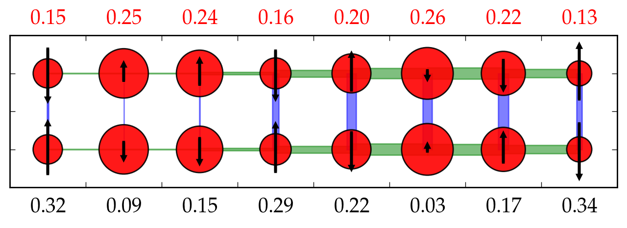
(c) $U/t=8$ $e_{\text{diff}}=-0.003$

Figure 4.12: Evolution of the inhomogeneous patterns and stabilities for $n=0.8,t^{\prime}=-0.2$ with respect to coupling strength. $e_{\text{diff}}=e_{8\times 2}-e_{4\times 4}$ for each point. At $U/t=8$, both 16-site fragments show inhomogeneous orders.

We also see from the results how the inhomogeneity develops with increasing interaction $U$. Fig. 4.12 shows the inhomogeneous patterns in $8\times 2$ fragments and their energies per site relative to those of $4\times 4$ fragments at the same doping ($x=0.2$) for $U/t$ from $4$ to $8$. The change in coupling strength results in stronger spin modulation and charge localization, and, at $U/t=8$ the pairing order also start to show inhomogeneity. At the same time, the $e_{\text{diff}}$ decreases from positive to negative values, indicating the inhomogeneous order is favored at stronger coupling.

It is important to note that the $8\times 2$ fragment geometry does not always lead to inhomogeneity, nor are all the $4\times 4$ fragments are homogeneous. (For instance, the same parameter as in Fig. 4.12(c) leads to an incommensurate inhomogeneous order in the $4\times 4$ fragment, while many $t^{\prime}=0.2$ calculations see homogeneous $8\times 2$ fragments.) Instead, at points where the tendency towards inhomogeneity is strong, we find a significant lowering of the energy associated with the inhomogeneous order, reflected either in a much lower energy of an inhomogeneous inhomogeneous $8\times 2$ fragment relative to the $4\times 4$ fragment, or inhomogeneity in both $8\times 2$ and $4\times 4$ fragments. Thus while it is not possible with our fragment sizes to extrapolate details of the inhomogeneities in the TDL (for example, the particular wavelengths of the spin, charge, and pairing instabilities, or diagonal versus vertical stripe patterns), the evidence points strongly to some forms of inhomogeneity surviving in the TDL at the indicated parts of the phase diagram.

Overall, in the underdoped regions of $U/t=8$ and $t^{\prime}=0$ and $-0.2$, various inhomogeneous orders are well established in $8\times 2$ and even $4\times 4$ fragment calculations, providing strong evidence to the inhomogeneity in the TDL; While at $U/t=6$, the calculations seem near the transition between the homogeneous and the inhomogeneous regimes, and give more ambiguous results, thus it is hard to determine what happens in the TDL ground state.

4.5 Conclusions

We have computed a ground-state phase diagram for the Hubbard model on the square lattice using cluster DMET. The accuracy achieved by DMET appears competitive with the exact ground-state benchmarks available at half-filling, while away from half-filling our error model suggests that the calculations remain very accurate. We observe AF and metallic phases and robust $d$-wave pairing. Further in parts of the phase space, our calculations strongly suggest that inhomogeneous phases are a feature of the thermodynamic limit, although the precise inhomogeneous patterns require larger clusters to resolve and reflect competition between different orders at very low energy scales.

However, for real materials such as the cuprates ($t\approx$3000K), the energy resolution achieved here for most of the phase diagram is already below the superconducting $T_{c}$, suggesting that the near degeneracy of competing orders will be lifted by terms beyond those in the Hubbard model, such as long-range charge and hopping terms, multi-orbital effects, and interlayer coupling. Moving beyond the Hubbard model to more realistic systems thus now appears of principal relevance.

Chapter 5 Stripe Order in the Underdoped Region of the Two-Dimensional Hubbard Model 

Competing inhomogeneous orders are a central feature of correlated electron materials including the high-temperature superconductors. The two-dimensional Hubbard model serves as the canonical microscopic physical model. Multiple orders have been proposed in the underdoped part of the phase diagram, which corresponds to a regime of maximum numerical difficulty.

In Chapter 4, we investigated the broad picture of the 2D Hubbard model phase diagram over a wide range of parameter space; In this chapter, we turn our focus on the strong-coupling, underdoped region of the phase diagram. We introduce a collaborative work with experts in various state-of-the-art numerical methods to perform exhaustive simulations to provide a definitive resolution of the order in the underdoped ground state of the strong coupling regime, which was left as an open question in Chapter 4. As we have shown before, the possible inhomogeneous orders are very rich and sensitive to slight changes in the parameters. Since it is a huge effort to deliver a detailed map for the ground-state orders, we focus on the $1/8$-doped point to demonstrate that it is possible to complete such a map with the latest development of numerical method.

At this point, We find a stripe order that has a highly compressible wavelength on an energy scale of a few Kelvin, with wavelength fluctuations coupled to pairing order. The favored filled stripe order is different from that seen in real materials, indicating the possibilities of other interactions beyond the Hubbard model at play. Our results demonstrate the power of modern numerical methods to solve microscopic models even in the most challenging settings.

In Sec. 5.1, we introduce the existing evidence and characterizations of the stripe orders. In Sec. 5.2, we discuss the numerical methods and data analysis techniques employed in the study. Sec. 5.3 presents the computational results, focusing on the competing orders in the $1/8$-doped Hubbard model at $U/t=8$, while in Sec. 5.4, we summarize the findings and discuss future directions.

5.1 Introduction

Competing inhomogeneous orders are a common feature in many strongly correlated materials [207]. A famous example is found in the underdoped region of the phase diagram of the high-temperature cuprate superconductors (HTSC). Here, multiple probes, including neutron scattering, scanning tunneling microscopy, resonant X-ray scattering, and nuclear magnetic resonance spectroscopy all lend support to various proposed inhomogeneous orders, such as charge, spin, and pair density waves, with suggested patterns ranging from unidirectional stripes to checkerboards [208, 209]. Recent experiments on cuprates indicate that the observed inhomogeneous orders are distinct from, and compete with, pseudogap physics [210, 211].

Much theoretical effort has been directed to explain the origin of the inhomogeneities [212]. Numerical calculations on microscopic lattice models have provided illuminating examples of the possible orders. The prototypical lattice model to understand HTSC is the 2D Hubbard model on the square lattice, with the Hamiltonian

$$\hat{H}=-\sum_{\langle ij\rangle,\sigma\in\{\alpha,\beta\}}ta^{\dagger}_{i\sigma}a_{j\sigma}+U\sum_{i}n_{i\alpha}n_{i\beta}$$ (5.1)

where $a^{(\dagger)}$ and $n$ denote the usual fermion creation, annihilation, and number operators, and $t$ and $U$ are the kinetic and on-site repulsion energies.

A large number of numerical techniques have been applied to compute the low-temperature and ground-state phase diagram of this model. Early evidence for unidirectional stripe ordering in the Hubbard model came from Hartree-Fock calculations [198, 213, 214, 215], while non-convex energy versus filling curves in exact diagonalization of small clusters of the related $t$-$J$ model were interpreted as signs of macroscopic phase separation  [216, 217]. Since then, inhomogeneous orders have been observed both in the Hubbard and $t$-$J$ models with density matrix renormalization group (DMRG)  [202, 67, 218], variational quantum Monte Carlo [219] and constrained path auxiliary field quantum Monte Carlo (AFQMC) [220], (iPEPS) [221], density matrix embedding theory (DMET) (see Chapter 4 and Ref. [92]), and functional renormalization group  [222] calculations amongst others, although not necessarily the same kind of inhomogeneity is observed in each case.

However, there are other sophisticated simulations, for example, with variational and projector quantum Monte Carlo [223, 224], and cluster dynamical mean-field theory, which do not see, or are unable to resolve, the inhomogeneous order [225, 2]. The most recent studies with iPEPS [221] and DMET [92], as well as some earlier variational calculations  [219, 226, 227, 228], further show that both homogeneous and inhomogeneous states can be observed and stabilized within the same numerical methodology, with a small energy difference between homogeneous and inhomogeneous states, on the order of $\sim 0.01t$ per site, corresponding to a smaller energy scale than the common cuprate superconductivity transition temperatures.

The small energy differences between orders means that very small biases in ground state simulations, such as from an incomplete treatment of fluctuations, using insufficiently accurate constraints to control the sign problem, bias towards low entanglement states, or from finite size effects, can easily stabilize one order over the other. Similarly, the low temperatures needed to resolve between orders is a challenge for finite temperature numerical methods  [64, 229].

However, in this work we will demonstrate that, with the latest numerical techniques, obtaining a definitive characterization of the ground state order in the underdoped region of the 2D Hubbard model is now an achievable goal. As a representative point in the phase diagram, we choose the iconic $1/8$ doping point at strong coupling ($U/t=8$). Experimentally, this doping corresponds to a region of maximal inhomogeneity in many HTSC’s, and in the strong coupling regime it is recognized as a point of maximum numerical difficulty and uncertainty in simulations [2].

Using state-of-the-art computations with detailed cross checks and validation, including newer methodologies such as infinite projected-entangled pair states (iPEPS) and density matrix embedding theory (DMET) as well as recent developments in established methodologies such as constrained-path auxiliary field quantum Monte Carlo (AFQMC) and density matrix renormalization group (DMRG), and with exhaustive accounting for finite size effects combined with calculations directly in the thermodynamic limit, we are able to achieve unprecedented accuracy in this challenging region of the ground-state phase diagram. In so doing, we can finally answer the question: what is the order and physics found in the underdoped ground state of the 2D Hubbard model?

5.2 Methods

5.2.1 Overview

An important new strategy we bring to bear on this part of the Hubbard model phase diagram is to combine the insights of multiple numerical tools with complementary strengths and weaknesses. This approach, pioneered in an earlier work on the Hubbard model [2], greatly increases the confidence of the numerical characterization. To understand what each method contributes, we briefly summarize the theoretical background and corresponding sources of error, and then discuss the detailed settings for each method in this work.

Auxiliary field quantum Monte Carlo.  AFQMC expresses the ground state of a finite system through imaginary time evolution (Eq. 2.47). The projection is Trotterized, and the evolution reduces to a stochastic single-particle evolution in the presence of auxiliary fields generated by the Hubbard-Stratonovich decoupling of the Hubbard repulsion. Away from half-filling, this decoupling has a sign problem. We use the constrained path (CP) approximation, to eliminate the sign problem at the cost of a bias dependent on the quality of the trial state [112, 230]. In this work, the Trotter error is well converged and we report the statistical error bar. To minimize the constrained path bias, we use several different trial states, including self-consistent optimization of the trial state [231]. The calculations are carried out on finite cylinders with open, periodic, and twist-averaged boundary conditions, with widths of up to 12 sites, and lengths of up to 72 sites. This method can reach large sizes and finite size effects are minimized. The uncontrolled error is from the CP approximation.

Density matrix renormalization group.  DMRG is a variational wavefunction approximation using matrix product states (MPS), which are low-entanglement states with a 1D entanglement structure. The quality of the approximation is determined by the bond dimension ($M$) of the MPS (Sec. 2.4.2). The calculations are carried out on finite cylinders with widths of up to 7 sites, and lengths of up to 64 sites, with periodic boundary conditions in the short direction and open boundaries in the long direction. Two different DMRG algorithms were used: one working in a pure (real-space) lattice basis, and another in a mixed momentum/lattice (hybrid) basis, with the momentum representation used along the short periodic direction [232]. We remove the bond dimension error and finite size error in the long direction by well-known extrapolation procedures, and report the associated error bar [233]. Consistency between the lattice and hybrid DMRG algorithms provides a strong validation of this error bar. The remaining uncontrolled error is the finite width error in the periodic direction.

Density matrix embedding. DMET is a quantum embedding method which works directly at the thermodynamic limit, although interactions are only accurately treated within a fragment (see Sec. 2.3) [54]. To solve for the ground state of the impurity model, consisting of a supercell of the original lattice (the fragment) coupled to a set of self-consistently determined bath orbitals, we use a DMRG solver [101]. We treat a series of fragment supercells with up to 18 sites ($9\times 2$) to target different low-lying states. With the narrow shapes of the fragments used in this work, we are able to perform DMRG calculations with negligible truncation errors; and we do not extrapolate the observables to the thermodynamic limit (with respect to the fragment sizes). Thus, the error bar reported in DMET only corresponds to the estimated error from incomplete self-consistency of the impurity problem (see Sec. 4.3). The remaining uncontrolled error is the finite fragment size error.

Infinite projected entangled pair states.  iPEPS is a variational approach using a low-entanglement tensor network ansatz natural to 2D systems [234, 235, 236]. The calculations are carried out directly in the thermodynamic limit where different supercell sizes including up to 16 sites (independent tensors that can break symmetry) are used to target different low-energy states. As in DMRG, the accuracy of the ansatz is systematically controlled by the bond dimension $D$ of the tensors. Estimates of quantities in the exact $D$ limit are obtained using an empirical extrapolation technique which is a potential source of uncontrolled error.

Cross-checks: systematic errors, finite size biases. The use of multiple techniques allows us to ameliorate the uncontrolled errors from one technique using information from another. For example, by carrying out simulations on the same finite clusters in the AFQMC and DMRG calculations, we can estimate the constrained path bias in AFQMC. Similarly, in the AFQMC calculations we can treat larger width cylinders than in the DMRG simulations; thus we can estimate the finite width error in DMRG. In other examples, DMRG may miss low-lying states with higher entanglement in finite bond dimension calculations. If, however, these states show up in other methods, we can control the initial boundary conditions or trial states of the DMRG calculations and target the missing states. These states may later show lower energy when extrapolated to infinite $M$.

In all of the methods, there is a bias towards orders commensurate with the shape of the simulation cell, be it the finite lattice and boundary conditions in AFQMC/DMRG, or the fragment cluster in DMET, or the supercell in iPEPS. Using this bias, together with different boundary conditions and pinning fields, we can stabilize different meta-stable orders. For example, by setting up clusters commensurate with multiple inhomogeneous orders and observing the order that survives, we can determine the relative energetics of the candidate states. We can fit the orders along the short axis or the long axis of the cluster to obtain two independent estimates of the energy. We have carried out exhaustive studies of about 100 different combinations of clusters, cells, and boundary conditions, to fully investigate the low-energy landscape of states.

To characterize the orders, we use the local hole density $h_{i}=1-(\langle n_{i\alpha}+n_{i\beta}\rangle)$, magnetic moment $m_{i}=\frac{1}{2}\langle n_{i\alpha}-n_{i\beta}\rangle$, and pairing order $\kappa_{ij}=\frac{1}{\sqrt{2}}(a_{i\alpha}^{\dagger}a_{j\beta}^{\dagger}+a_{j\alpha}^{\dagger}a_{i\beta}^{\dagger})$ ($i$ adjacent to $j$).

5.2.2 Detailed Specifications

In this section, We discuss the process, scope and computational parameters used in each of the computational methods in detail.

Auxiliary field quantum Monte Carlo

Two sets of AFQMC calculations are performed using the constrained-path AFQMC method with self-consistently optimized, unrestricted Hartree-Fock trial wavefunctions [231].

The first set is on cylinders of dimension $L_{x}\times L_{y}$ ($L_{x}>L_{y}$) with open boundary conditions (OBC) along the $x$-direction and periodic boundary conditions (PBC) along the $y$-direction. This allows the AFQMC calculations to be directly compared with DMRG results. We also run calculations with pinning fields to fix the desired spin structures. Several types of antiferromagnetic (AF) pinning fields are applied along the open edges of the cylinders depending on the target state. The types of pinning fields include: the in- and anti-phases pinning fields along the two boundaries, and the pinning fields applied to only one edge.

With in- (anti-) phase pinning fields, we target an odd (even) number of nodes (where the $\pi$-phase shift happens) in the system ($L_{x}$ is always even in the calculations); while pinning fields on only one edge are able to accommodate states with different wavelengths so we can learn which wavelength survives in the competition. The strength of the pinning fields is $|h|=0.5t$ for all calculations.

In the second set of calculations, we use PBC or twist averaged boundary conditions (TABC) along both directions. The twist averaging allows us to reduce the finite size errors in the total energy, thus giving a more unbiased estimation of the energy order for various low-lying states.

For $U/t=8$, the wavelength 5, 6, 8, 10 and 12 stripes are explicitly studied in AFQMC using cylinders, while the energy estimates from PBC and TABC calculations are obtained for wavelengths 5 to 10. Similar calculations are also performed at $U/t=6$ and $U/t=12$.

Density matrix renormalization group in the lattice basis

Lattice-basis DMRG calculations are carried out on cylinders of size $L_{x}\times L_{y}$ ($L_{x}>L_{y}$) as well. Both fixed particle number (at $1/8$ doping) and broken particle-number symmetry calculations are conducted.

To stabilize the states with particular wavelengths, we use as initial states product states with holes in the desired locations, and apply temporary fields and (site-dependent) chemical potentials on the whole cylinder in the first few sweeps. A temporary chemical potential $\mu=2.0$ is applied on the sites where the holes are supposed to be in the final striped state, and a temporary magnetic field of strength $|h|=0.5$ is applied to fit the antiferromagnetic domains between holes. After the first few sweeps (typically up to bond dimension $M=600$) the temporary field and chemical potential are turned off, and the state is called “stable” in the DMRG simulation if it keeps the same wavelength during subsequent sweeps. In some cases, an AF pinning field of strength $|h|=0.5$ at the open edges is kept in the full simulation to further stabilize the state. By extrapolating to the infinite length, the pinning field does not affect the energy per site at the thermodynamic limit.

We next consider the pairing order. To measure the pairing order, we simulate the Hubbard cylinder in the grand canonical ensemble, i.e., without particle number conservation. The chemical potentials are tuned so that the expectation value of the particle number is close to the desired value ($7/8$ of the number of sites). We apply pairing pinning fields at the edges, to induce broken particle-number symmetry, and observe how the pairing order decays into the bulk.

The lattice-basis DMRG simulations are carried out at $U/t=8$ and $U/t=12$, the width 4, 6 and 7 cylinders to simulate stripes of various wavelengths.

Density matrix renormalization group in the hybrid basis

Again, the hybrid-basis DMRG calculations are carried out on cylinders of size $L_{x}\times L_{y}$, with OBC in the longitudinal $x$-axis and PBC or APBC in the transverse $y$-direction.

The DMRG algorithm in a mixed–real-momentum-space (hybrid) representation [232] is used. The hybrid-basis DMRG algorithm uses a real-space representation in the longitudinal cylinder direction and a momentum-space representation in the transverse direction. The additional transverse-momentum quantum number grants us a speedup over lattice-basis DMRG whose cost grows with the width of the cylinder. For width-6 Hubbard cylinders, the hybrid-space algorithm is approximately 20 times faster than its real-space counterpart.

To obtain the ground-state energy for fixed $L_{y}$ (while $L_{x}$ is infinite), we perform consecutive extrapolations first in the DMRG truncation error $\Delta w$ and then in the inverse cylinder length $1/L_{x}$.

In order to directly target and stabilize different stripe configurations on width-6 cylinders with PBC, we use a sine-shaped pinning field coupled to the local charge density

$$P=\sum_{x\,y\,\sigma}A\cos(k_{x}\,x\,+\,\phi_{0})n^{\vphantom{\dagger}}_{x\,y\,\sigma}$$ (5.2)

with suitable amplitude $A$, wave vector $k_{x}$, and phase $\phi_{0}$. Note that the pinning field only acts on the charge density, while does not explicitly break the spin or particle-number symmetries. The contribution to the ground-state energy, $\langle\Psi_{0}|P|\Psi_{0}\rangle$, is subtracted after the DMRG calculation. We found a field amplitude of $A=0.01$ to be sufficient to stabilize the different stripe patterns and to improve the convergence of the DMRG algorithm. After the calculations are converged, the charge order can be measured directly from the one-body density matrix, while the spin structure factor and pairing correlation functions are measured to obtain the spin and pairing order.

The calculations are carried out on width 4 to 8 cylinders of various lengths. However, for width 8, we do not achieve sufficient convergence in terms of DMRG density matrix truncation, despite using up to $M=35000$ states.

Density matrix embedding theory

We perform the DMET calculations on an auxiliary square lattice of dimension $L\times L$, where $L=160$ for most fragment sizes ($L=168$ for $7\times 2$ fragments and $L=162$ for $9\times 2$ fragments). The correlation potential is allowed to break spin and particle-number symmetries, and so do the impurity model wavefunctions. The calculations are carried out as described in Appendix B.2, and similar to those in Chapter  4, but a larger number of fragment sizes, shapes and boundary conditions are explored. Various shapes of fragments are used to accommodate uniform $d$-wave order, vertical and diagonal stripes. The shapes of the fragments are summarized in Fig. 5.1. We do not attempt to do extrapolations of fragment size in this work but compare the energies of different fragments directly. This is making an implicit assumption that the finite size errors are about the same for different fragment shapes employed here, and this lack of TDL extrapolation is the main systematic error. In our experience, however, it is reasonable to directly compare energies of fragments of the same orientation and family (e.g. $L\times 2$), which is confirmed in this work by comparison with the other techniques.

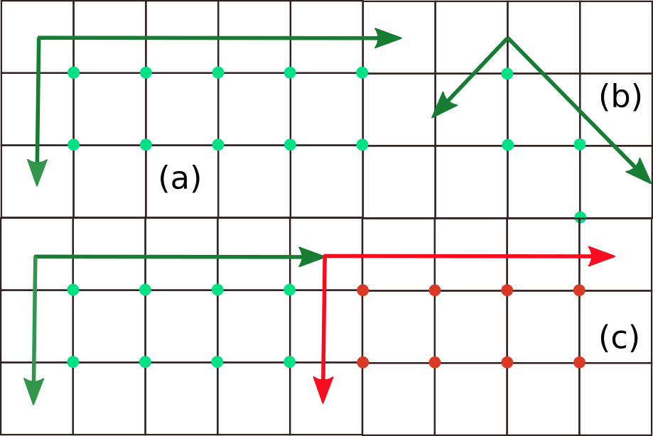
Figure 5.1: Fragment shapes used in the DMET calculations: (a) $\lambda\times 2$ fragments. (b) $\lambda\sqrt{2}\times\sqrt{2}$ fragments. (c) $\lambda\times 2$ fragments with spin inversions on neighboring supercells.

$\lambda\times 2$ cells [Fig. 5.1(a)] are used to study vertical stripes with odd wavelengths. As the AF order has a $\pi$-phase shift at the domain wall, the AF order is commensurate with the cell size. For even-wavelength stripes, the setup is similar, however, to support a single domain wall, it is necessary for the spin wavelength to be twice that of the charge wavelength. To allow this, rather than using a large cluster of size $2\lambda\times 2$, we modify the way the correlation potential is added to the lattice wavefunction, i.e. by swapping the spin channels between neighboring cells in the longitudinal direction [Fig. 5.1(c)], so translation by a unit cell gives a time reversal, $n_{i\alpha}\to n_{i\beta}$ transformation. Specifically, the local correlation potential in this case is written as

$$u=\sum_{C_{1}}\sum_{i,j\in C_{1}}(\sum_{\sigma}u_{ij\sigma}a_{i\sigma}^{\dagger}a_{j\sigma}+\Delta_{ij}a_{i\alpha}^{\dagger}a_{j\beta}^{\dagger}+c.c.)+\sum_{C_{2}}\sum_{i,j\in C_{2}}(\sum_{\sigma}u_{ij\bar{\sigma}}a_{i\sigma}^{\dagger}a_{j\sigma}+\Delta_{ij}^{\prime}a_{i\alpha}^{\dagger}a_{j\beta}^{\dagger}+c.c.)$$ (5.3)

where $C_{1}$ and $C_{2}$ label even and odd cells along the longitudinal $x$ direction. Both $\Delta^{\prime}=\pm\Delta$ possibilities are tested in our calculations, because we cannot determine the phase factor associated with the transformation

$$a_{i\alpha}\rightarrow a_{i+R,\beta},a_{i\beta}\rightarrow\pm a_{i+R,\alpha}.$$

where the $R$ denotes translation by a unit cell. As shown in the results, neither parameterization results in finite pairing order in the ground-state of even wavelength stripes. This trick not only greatly reduces the computational cost it would have taken to simulate the even-wavelength stripes, but also makes the energies of odd and even wavelengths more comparable.

We also use the traditional cells in Fig. 5.1(a) for even wavelengths to simulate possible spin density wave states. One of these states turns out to have lower energy than the stripe of the same wavelength at $U/t=6$.

We also use the tilted clusters in Fig. 5.1(b) to accommodate diagonal stripes. As the finite-size effects are different in regular and tilted clusters, we use both $2\times 2$ and $2\sqrt{2}\times\sqrt{2}$ clusters to obtain the uniform $d$-wave state, to estimate the relative energies of the states on regular and tilted lattices.

In all the calculations reported in this work, the DMRG solution of the impurity model is converged in terms of truncation error, and the DMET uncertainty comes solely from the convergence of the correlation potential. We report the energy and its uncertainty as the average and half of the difference of the last two DMET cycles, respectively.

Infinite projected entangled-pair state

An infinite projected entangled-pair state (iPEPS) [234, 237, 238] (also called a tensor product state [239, 235]) is an efficient variational tensor network ansatz for two-dimensional states in the thermodynamic limit which obeys an area law of the entanglement entropy [240]. The ansatz consists of a supercell of tensors which is periodically repeated on a lattice, with one tensor per lattice site. Each tensor has a physical index which carries the local Hilbert space of a lattice site and four auxiliary indices which connect to the nearest-neighboring tensors on a square lattice. Each auxiliary index has a certain dimension $D$, called the bond dimension, with which the accuracy of the ansatz (the number of variational parameters) can be controlled systematically. An iPEPS with $D=1$ corresponds to a product state, and by increasing $D$ entanglement can be systematically added. In this work we use bond dimensions up to $D=16$ corresponding to highly-entangled states.

For translationally invariant states a supercell with only a single tensor is needed. If the translational symmetry is spontaneously broken a supercell compatible with the symmetry breaking pattern is required. For example, a Néel ordered state requires a supercell with two different tensors $A$ and $B$ (one for each sublattice), or a stripe state with period 5 requires a $5\times 2$ supercell with 10 independent tensors. A diagonal stripe state with period $L/\sqrt{2}$ can be obtained in a $L\times L$ rectangular supercell, or more efficiently by using a $L\times 1$ supercell with $L$ different tensors and translation vectors $v_{1}=(L,0)$, $v_{2}=(1,1)$.

By running simulations with different supercell sizes one obtains different competing low-energy states. In order to determine which of these competing low-energy states corresponds to the true ground state a systematic analysis of the energy as a function of $D$ is required. Here we used the extrapolation technique from Ref. [4] in which the energy is plotted as a function of the so-called truncation error $w$ in the simulation, and then the extrapolation to the $w\rightarrow 0$ limit is taken to determine the energy of each of the competing states. While in 2D it is theoretically unknown how the energy depends on $w$, several benchmarks [4] have empirically shown that an accurate estimate can be used using a polynomial fit.

In this work the optimization of the tensors has been done using an imaginary time evolution based on the so-called full update [241] (or fast-full update [242]), which is more accurate than the simple update approach [243]. Observables are evaluated by contracting the two-dimensional tensor network in a controlled, approximate way, using a variant [205, 221] of the corner-transfer matrix (CTM) method [244, 245]. The accuracy of the contraction is controlled by the “boundary” dimension $\chi$, which is chosen large enough such that the resulting error is small (compared to the effect of the finite $D$). To increase the efficiency we make use of Abelian symmetries [246, 247]. Fermionic statistics are taken into account following the formalism explained in Refs  [248, 241].

5.2.3 Estimating Long-range Coulomb Interaction

We estimate the long-range Coulomb interactions of various low-lying states to understand how these interactions may change the relative order of the states in real cuprates. We use charge order from DMET calculations, and compute

$$e_{\text{Coul}}=\frac{1}{N_{c}}\sum_{i\in\text{frag},j,i\neq j}(h_{i}-\bar{h})(h_{j}-\bar{h})/4\pi\varepsilon_{0}\varepsilon r_{ij}$$ (5.4)

where $N_{c}$ is the size of the fragment, $h_{i}$ is the hole density on site $i$, and $\bar{h}$ is the average hole density ($1/8$).

In atomic units, i.e. if we express the energy in Hartrees, and distance in Bohr, $1/4\pi\varepsilon_{0}=1$. The appropriate dielectric constant to use in a statically screened Coulomb interaction in the CuO₂ plane has been estimated to lie between about $4$ and $27$  [249, 250]. We use a dielectric constant of $\varepsilon=15.5$, and a lattice constant $a=3.78$Å$=7.14\text{ Bohr}$ corresponding to the lattice constant of La₂CuO₄. We transform the computed Coulomb energy (per site) to units of $t$, using $t\sim 3000K\sim 0.01\text{ Hartree}$.

In 2D, the Coulomb summation converges reasonably fast. We choose a cutoff radius as 300 lattice spacings and converge the Coulomb energy to the fourth digit in units of $t$. This is of course just a crude, order of magnitude estimate, because we neglect the effect of relaxation in the presence of the Coulomb interaction, and there is significant uncertainty in the dielectric.

5.3 Results

Using the above methods, we carry out calculations for the ground state of the 2D Hubbard model at $1/8$ doping at $U/t=8$. The first check of reliability is the independent convergence of the methods for the energy per site. While the quality of the ground-state energy may be a poor proxy for the quality of the corresponding state when the overall accuracy is low (as there are always many degenerate states far above the ground state), well-converged energies are a much tighter constraint on the ground state order, as any degeneracies must be below the energy convergence threshold.

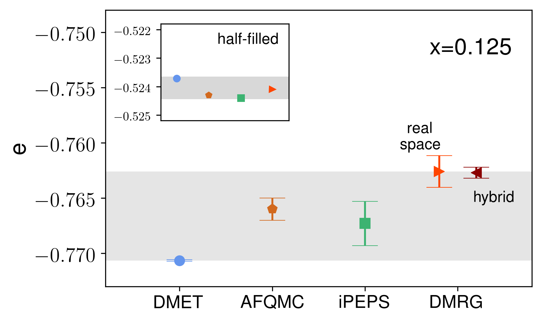
Figure 5.2: Best estimates of ground state energies per site for the $1/8$-doped 2D Hubbard model at $U/t=8$ from DMET, AFQMC, iPEPS and DMRG. Inset: Best estimates of ground state energy for the half-filled 2D Hubbard model at $U/t=8$. Here and elsewhere in this chapter, error bars indicate only the estimable numerical errors of each method; uncontrolled systematic errors are not included.

Fig. 5.2 shows the best energy estimate for the ground state from the different methods. The two different DMRG formulations (real space and hybrid basis) agree perfectly, providing a strong independent check of the calculations, and in subsequent figures we report only the single consistent result. Note that the error bars for AFQMC, DMRG, and DMET do not reflect the uncontrolled systematic errors in the methods. However, as described above, the systematic errors can be estimated by cross checks between the methods. For example, DMRG and AFQMC calculations on finite clusters with identical boundary conditions provide an estimate of the small constrained path bias (see Table 5.1 and Ref. [231]) consistent with the difference in the DMRG and AFQMC energies in Fig. 5.2 (around $0.0035t$); similarly AFQMC extrapolations to the thermodynamic limit indicate that the DMRG energies (using cylinders up to width 7) are essentially converged with respect to cylinder width (Fig. 5.3).

Table 5.1: Comparison of energies per site from AFQMC and DMRG for various inhomogeneous states on cylinders with pinning fields. The CP-error denotes the energy difference between AFQMC and DRMG results, as a result of the constrained path error. Note the wavelength-5 stripes are meta-stable.

Size	Stripe wavelength	DMRG	AFQMC	CP-Error
$4\times 16$	8	-0.77127(2)	-0.7744(1)	-0.0031
$6\times 16$	5	-0.7682(3)	-0.7692(1)	-0.0010
$6\times 16$	8	-0.7691(5)	-0.7725(2)	-0.0034
$4\times 24$	8	-0.76939(3)	-0.7727(2)	-0.0033
$6\times 32$	5	-0.7648(3)	-0.7663(1)	-0.0015
$6\times 32$	8	-0.7658(7)	-0.7691(2)	-0.0033

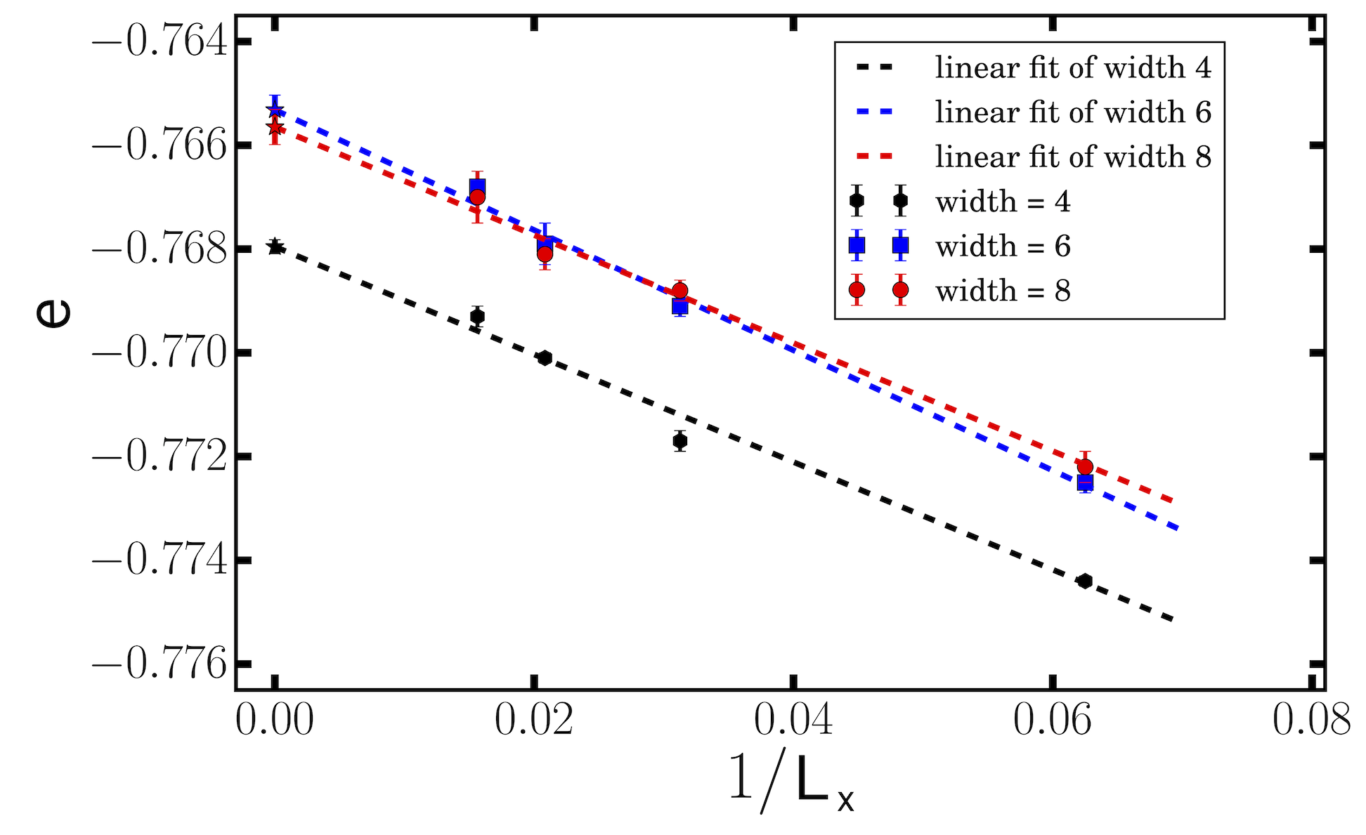
Figure 5.3: Energies per site for wavelength-$8$ stripes in various cylinder sizes for $U/t=8$. Pinning fields are applied on the open boundaries. Linear fits of $1/L_{x}$ are shown. The infinite length values and error bars from extrapolation are marked as stars in the plot.

The ground-state energy has close agreement between all the methods, and all energies lie in the range $-0.767\pm 0.004t$. If, for a typical HTSC material, we estimate $t\sim 3000K$, then this corresponds to a range of about $\pm 10K$ per site, or $\pm 100K$ per hole. For a numerical comparison, this is also more than an order of magnitude lower than the temperatures accessible in finite temperature, thermodynamic limit, simulations in this part of the phase diagram, indicating that we are potentially accessing different physics from what haven been seen before [2, 229]. Shown in the inset are the corresponding best estimates at half filling from the same methods, where the spread in energies is less than $0.001t$. This illustrates the significantly greater numerical challenge encountered in the underdoped region. Nonetheless, the accuracy and agreement reached here represents a ten-fold improvement over recent comparisons of numerical methods at this point in the phase diagram [2].

Ground state stripe order. For all the methods employed, the lowest energies shown in Fig. 5.2 correspond to a vertical striped state. This corresponds to a co-directional charge and spin-density wave, with the region of maximum hole density coinciding with a domain wall and $\pi$-phase shift in the antiferromagnetism. As mentioned, unidirectional stripes of various kinds are a long-standing candidate order in the doped Hubbard and related models. Hartree-Fock calculations give filled stripes (i.e. one hole per charge unit cell) in both vertical and diagonal orientations, while one of the first applications of the DMRG to 2D systems found strong evidence for half-filled stripes in the $t$-$J$ model [202]. Finally, one of the earliest examples of inhomogeneity in doped HTSC’s were the static half-filled stripes in LaSrCuO at 1/8 doping  [251].

The convergence to the same inhomogeneous order in the ground state in the current study, from multiple methods with very different approximations, strongly suggests that stripes indeed represent the true ground state order of the Hubbard model in the underdoped regime, and further highlights the accuracy we achieve with different techniques. However, the stripe order we observe has some unusual characteristics. We return to the details of the stripe order, its associated physics, and its relationship with experimentally observed stripes further below. First, however, we examine the possibility of other competing meta-stable states.

Competing states: uniform $d$-wave state. Recent work using iPEPS and DMET on the $t$-$J$ and Hubbard models suggested close competition between a uniform $d$-wave superconducting ground state and a striped order [221, 92]. With an improve energy resolution in this work, uniform states did not spontaneously appear in any of our calculations which indicates that they lie higher in energy than the striped order. We found that we could stabilize a uniform $d$-wave state in the DMET calculations by constraining the fragment to a $2\times 2$ or $2\sqrt{2}\times\sqrt{2}$ geometry [Fig. 5.4(b)] and in the iPEPS calculations by using a $2\times 2$ unit cell [Fig. 5.4(c)]. DMET calculations on similarly shaped larger clusters (such as a $4\times 4$ cluster) spontaneously broke symmetry to create a non-commensurate non-uniform state. From these calculations we estimate that the uniform state lies $\sim 0.01t$ above the lowest energy state [Fig. 5.4(a)], and is not competitive at the energy resolution we can now achieve.

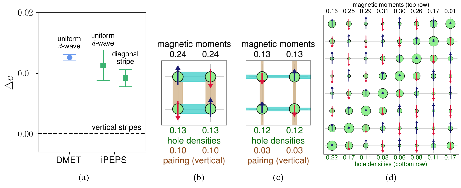
Figure 5.4: Important candidate states relative to the striped ground state from DMET and iPEPS and the orders. (a) Relative energy of competing states compared to the vertical striped state. Charge, spin and pairing orders of the uniform $d$-wave state from (b) DMET and (c) iPEPS. (d) Charge and spin orders of the diagonal striped state from iPEPS. Note that the spins are flipped in the neighboring supercells. (Circle radius is proportional to hole density, arrow height is proportional to spin density, bond width is proportional to pairing density).

Competing states: diagonal stripes. While we find the ground state order to be a vertical stripe type order, other studies of stripes indicate that different orientations can form [175]. On short length scales, the relevant question is whether diagonal stripes [with a $(\pi,\pi)$ wave vector] are competitive with vertical stripes [with a $(0,\pi)$ wavevector]. With the boundary conditions used in this work, diagonal stripes would be frustrated in the DMRG and AFQMC calculations, and did not spontaneously appear. To stabilize diagonal stripes in the DMET and iPEPS calculations, we used tilted $n\sqrt{2}\times\sqrt{2}$ fragments ($n=2,5)$ for DMET, and a $16\times 16$ simulation cell with 16 independent tensors in iPEPS. The $16\times 16$ iPEPS cell gave a diagonal stripe [Fig. 5.4(d)] that was significantly higher in energy than the vertical stripe, by $0.009t$. The DMET cluster gave rise to a frustrated diagonal order that we also estimate to be higher in energy by $\sim 0.005t$. While it is likely that the orientation of the stripe will depend on doping and coupling, vertical stripes appear to be significantly preferred at this point in the phase diagram.

Competing states: other short-range orders. While other types of order have been proposed in the underdoped region, such as spiral magnetic phases [171, 222] and checkerboard order [252], we find no evidence for other kinds of short-range orders at this point in the phase diagram from any of our methods. The lack of checkerboard order, which would easily fit within the large clusters in our simulations (e.g. up to $64\times 6$ in the DMRG calculations) appears to rule them out as low energy states, in agreement with earlier DMRG simulations on the $t$-$J$ model [253]. While we cannot rule out incommensurate orders, we have found that the variation of energy with unit cell wavelength (see below) is quite smooth, thus we do not expect a dramatic energy gain from incommensurability. We note that studies finding incommensurate magnetic orders have focused on smaller values of $U$ [222].

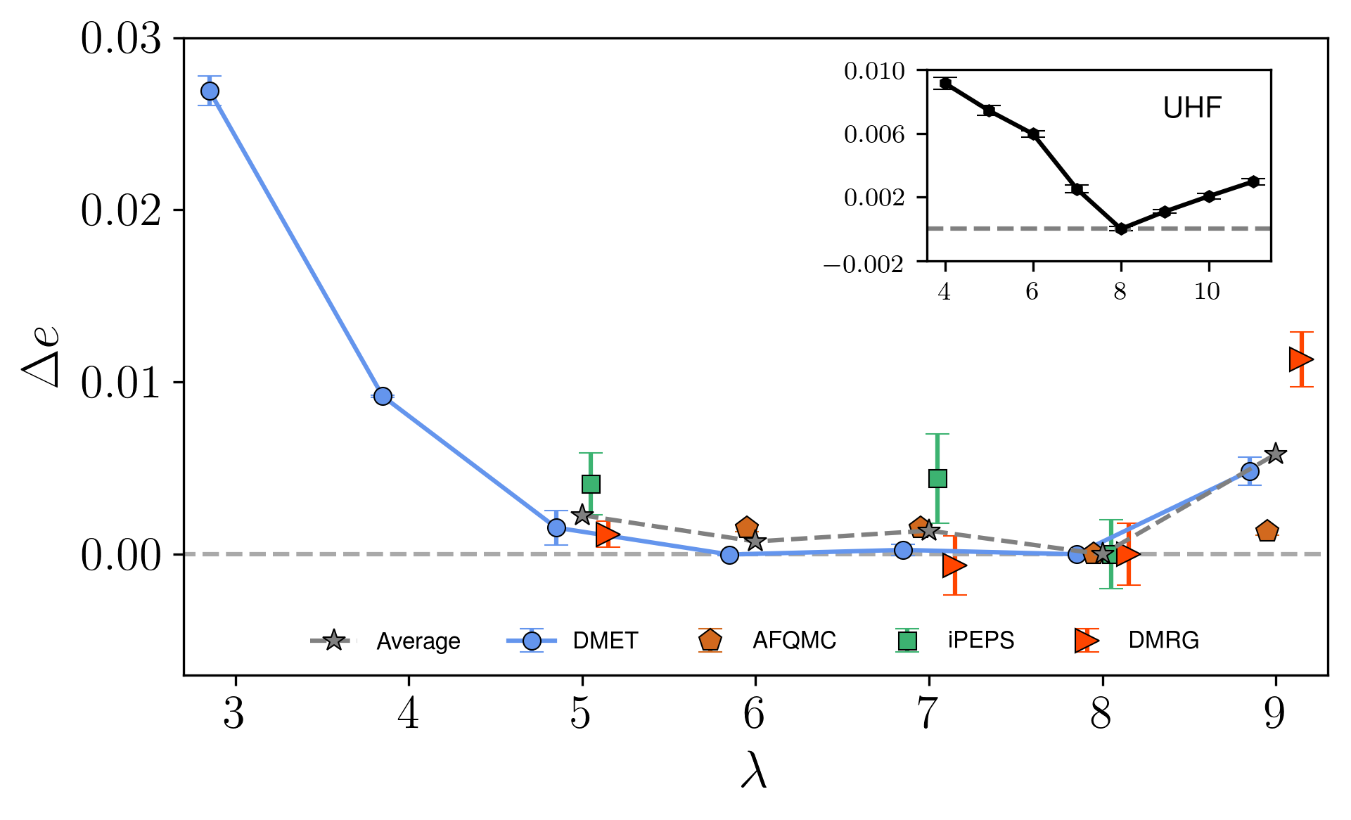
Figure 5.5: Energies per site for stripes with different wavelengths relative to that of the wavelength-8 stripe from DMET, AFQMC, iPEPS and DMRG. To aid readability, the data points are shifted horizontally. Inset: Relative energies of stripes with different wavelengths from UHF, with an effective coupling $U/t=2.7$ obtained from self-consistent AFQMC simulations.

Ground state stripes: detailed analysis. We now return to a more detailed discussion of the vertical stripe order observed in the ground state. Within the family of vertical stripes, we can consider questions of wavelength (charge and spin periodicity), type and strength of charge and spin modulation (e.g. bond- versus site-centered), and coexistence with pairing order.

We first discuss the wavelength $\lambda$. At $1/8$ doping, the filling of the stripe is related to the wavelength by $\lambda/8$. As described, we can access different wavelength meta-stable stripes and their relative energetics by carefully choosing different total cluster dimensions and boundary conditions (in the DMRG and AFQMC calculations) or unit cell/fragment sizes (in the iPEPS and DMET calculations). Fig. 5.5 shows the energy per site of the stripe versus its wavelength $\lambda$ from the multiple methods. Earlier DMRG calculations on the Hubbard model had focused on $\lambda=4$ (half-filled stripes) which are seen in HTSC’s [202, 67], but we now observe that these are relatively high in energy. A striking feature is that for $\lambda=5-8$ the energies are nearly degenerate. This is clearly seen in the DMET data where stripes of all wavelengths can be stabilized, as well as the plot of the averaged energy of the methods between $\lambda=5-8$.

The energy difference between the $\lambda=5$ and $\lambda=8$ stripe in the different methods is estimated to be between $0.0005t$ (DMRG)–$0.0041t$ (iPEPS) with an average of $0.0022t$. This suggests that the magnetic domain walls can fluctuate freely, consistent with proposals for fluctuating stripes [210]. In particular, the stripes may be distorted at a small cost over long length scales.

Although the different wavelengths are nearly degenerate, there appears to be a slight minimum near wavelength $\lambda=8$ (a filled stripe) in all the methods. Very recently, similar filled stripes have been reported as the ground state in part of the frustrated $t$-$J$ model phase diagram [254]. $\lambda=9$ appears significantly higher in energy in both DMET and DMRG. In the DMRG calculations, the $\lambda=9$ state was not even meta-stable as boundary conditions and initial states were varied, so the high-energy state shown was forced with a static potential. The AFQMC results show a much weaker dependence on wavelength for longer wavelengths, for example the $\lambda=8$ and $\lambda=10$ stripe energies per site appear to be within $0.0015t$. However, when a mixture of the $\lambda=8$ and $\lambda=10$ stripe states is set up on a length 40 cluster that is commensurate with both, the state that survives is the $\lambda=8$ stripe, suggesting a preference for this wavelength. The increase in energy at wavelengths $\lambda>8$ coincides with unfavorable double occupancy of the stripe. This simple interpretation is supported by a mean-field (unrestricted Hartree-Fock (UHF)) calculation with an effective interaction $U/t=2.7$ chosen within the self-consistent AFQMC procedure. The mean-field result shows a clear minimum at a wavelength-$8$ vertical stripe. (Note that this requires the use of an effective $U/t$; at the bare $U/t=8$, mean-field theory would produce a diagonal stripe [255].) The correspondence between the energies and densities in the effective mean-field and correlated calculations suggests that the mean-field theory with a renormalized interaction may be surprisingly good at describing the energetics of stripes. However, mean-field theory appears to somewhat underestimate the degeneracy of the stripes as a function of wavelength, particularly at shorter wavelengths.

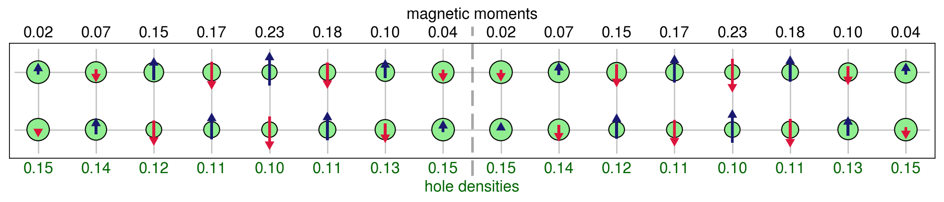
(a) AFQMC

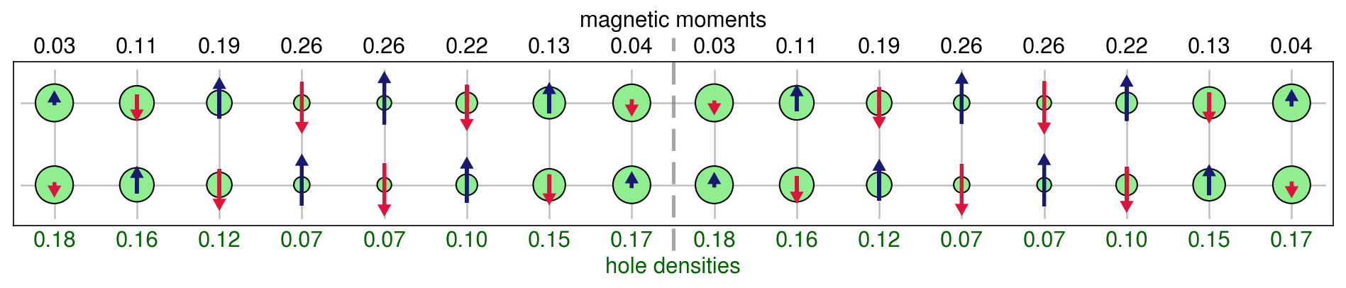
(b) DMRG

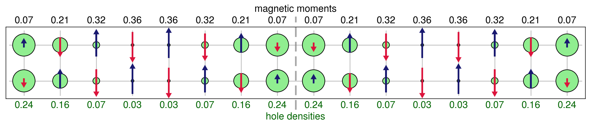
(c) DMET

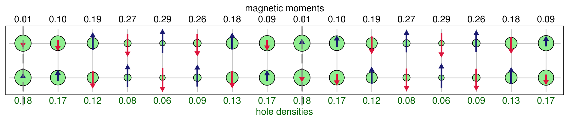
(d) iPEPS

Figure 5.6: Charge and spin orders in the wavelength-8 stripes from AFQMC, DMRG, DMET and iPEPS. The local magnetic moments and hole densities are shown above and below the order plots, respectively. (Circle radius is proportional to hole density, arrow height is proportional to spin density). The gray dashed lines represent the positions of maximum hole density.

The stripe order for the $\lambda=8$ stripe from the different methods is depicted in Fig. 5.6. We show the full period (16) for the spin modulation. The stripe is bond-centered in the AFQMC, DMRG, and DMET calculations. In the iPEPS calculation, the stripe is nominally site-centered. In all the calculations, the width of the hole domain wall spans several sites, blurring the distinction between bond- and site-centered stripes, and we conclude that the energy difference between the two is very small. There is substantial agreement in the order observed by the different numerical techniques, with only some differences in the magnetitude of modulation of the hole and spin-densities.

Note that for even-wavelength stripes, the spin wavelength must be twice that of the charge modulation in order to accommodate the stripe as well as the antiferromagnetic order. At odd wavelengths, site-centered stripes appear in all the calculations, and here charge and spin order can have the same wavelength. (This odd-even alternation does not affect the peaks of the structure factor near $(\pi,\pi)$, see Appendix 5.A.1.)

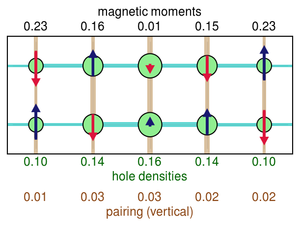
(a) iPEPS $\lambda=5$

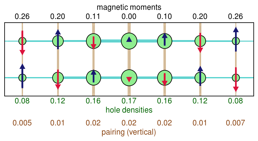
(b) iPEPS $\lambda=7$

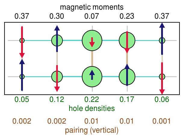
(c) DMET meta-stable $\lambda=5$

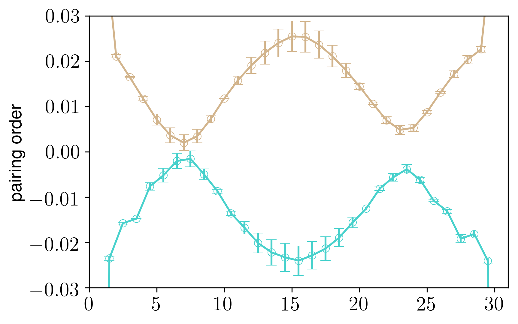
(d) DMRG pairing order parameters

Figure 5.7: Meta-stable stripe states with $d$-wave pairing from iPEPS, DMET, and DMRG. (a)(b) iPEPS stripes with $\lambda=5$ and $\lambda=7$. (c) DMET meta-stable $\lambda=5$ stripe with pairing. (Circle radius is proportional to hole density, arrow height is proportional to spin density, bond width is proportional to pairing density). (d) DMRG pairing order parameters on a 32$\times$4 cylinder. The positive values are from the vertical bonds and the negative values from the horizontal bonds.

Pairing order, fluctuations, and superconductivity. A key question is whether pairing order coexists with stripe order. Previous work on the $t$-$J$ model with iPEPS found coexisting $d$-wave order for partially filled ($\lambda<8$) stripes. No $d$-wave order is found in the Hubbard $\lambda=8$ stripe with any technique. However, $d$-wave order can be found at other wavelengths. For example, for $\lambda=5$ and $\lambda=7$ stripes, iPEPS produces $d$-wave order along the bonds (see Fig. 5.7) with a maximum $d$-wave expectation value of $0.026$ and $0.021$, respectively. DMRG calculations with pinning pairing fields on the boundary for a $32\times 4$ cylinder also find $d$-wave order, with an extrapolated maximum $d$-wave order of $0.025$, consistent with the iPEPS results. In the DMET calculations, though the lowest energy $\lambda=5$ stripe has no $d$-wave order, however, at slightly higher energy ($\sim 0.003t$) a $\lambda=5$ state similar to the iPEPS stripe can be found with coexisting $d$-wave order, but with a substantially smaller maximum order parameter of $0.01$. Overall our results support the coexistence of modulated $d$-wave order with the striped state, although the strength of pairing is intertwined with the stripe wavelength and filling. The pairing modulation we find (Fig. 5.7) is in phase between cells. Other kinds of pairing inhomogeneities, such as pair density waves, have also been discussed in the literature [212].

It has long been argued that fluctuating stripes could promote superconductivity [256, 257, 258]. Our work provides some support for this picture, as there is a low energy scale associated with the deformation of stripe wavelength while we also find coupling between the wavelength and the pairing channel. We can imagine fluctuations in wavelength both at low temperatures, as well as in the ground state. In the latter case, this could lead to a stripe liquid ground state rather than a stripe crystal. Our calculations are consistent with both possibilities.

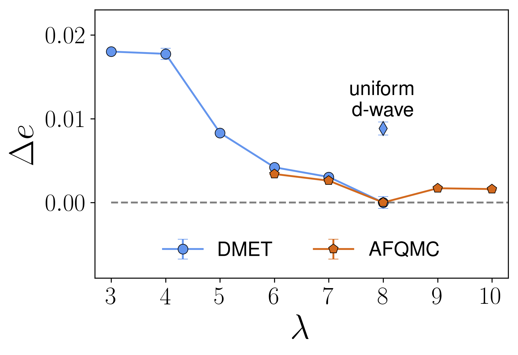
(a) $U/t=6$

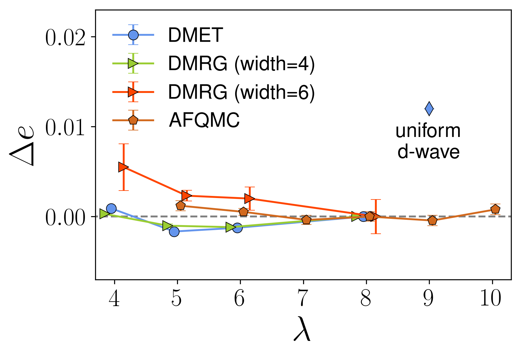
(b) $U/t=12$

Figure 5.8: Relative energies of stripe states (with respect to wavelength) and the uniform $d$-wave state with $1/8$ doping at weaker and stronger couplings.

Changing the coupling. We may also ask whether the $U/t=8$, $1/8$ doping point is an anomalous point in the Hubbard phase diagram, and, if, for example, moving away from this point would alleviate the unusual stripe compressibility (with respect to wavelength at fixed doping) that we observe. In Fig. 5.8 we show the energies of various striped states and the uniform state at $U/t=6$ and $U/t=12$, $1/8$ doping, computed using AFQMC, DMET and DMRG. At both couplings, the stripes around wavelength 8 are nearly degenerate, with the degeneracy increasing as the coupling increases. At $U/t=6$, we find the ground state is a filled stripe state with wavelength $\lambda=8$, with a larger energy stabilization than at $U/t=8$. The trend is consistent with the state observed at $U/t=4$ with a more sinusoidal spin-density wave, more delocalized holes, and a more pronounced minimum wavelength  [220]. In particular, at $U/t=6$, at $\lambda=4$, the stripe and spin-density wave state (distinguished by whether or not the state has the $\pi$-phase shift) are essentially degenerate in DMET [$e=-8589(6)$ vs. $e=-0.85890(4)t$], compared to an energy difference of $\sim 0.009t$ at $U/t=8$. At $U/t=12$, we find a filled stripe with AFQMC and DMRG (width 6), but DMET and DMRG on a narrower cylinder (width 4) find $\lambda=5-6$. The similarity of the DMET and DMRG (width 4) data suggests that the shorter wavelength is associated with a finite width effect. We notice that $2/3$-filled stripes consistent with $\lambda=5-6$ were also seen in earlier DMRG studies on width-6 cylinders [218], but a more detailed analysis shows that the filled stripe becomes favored when extrapolated to infinite bond dimension. In fact, similar to Ref. [218], at finite $M$, we always have the $2/3$-filled stripes as the ground state because of their lower entanglement than the filled stripes. We are only able to stabilize the filled stripes, which turns out to be the true ground state when having eliminated the density matrix truncation error, by initializing the DMRG calculations with favorable initial guess, based on our understanding of the model and with the help of information from other methods. This example again illustrates the benefits of combining information from different numerical methods. Thus, we conclude that the ground state at $U/t=12$ is also the $\lambda=8$ stripe, although stripes of other wavelengths become even more competitive than at $U/t=8$. Overall, the similarity in the physics over a wide range of $U/t$ indicates that striped orders with low energy fluctuations of domain walls remain a robust feature in the moderate to strongly coupled underdoped region.

Connection to stripe order in HTSC’s. In HTSC’s the accepted stripe wavelength at 1/8 doping (e.g. in LaSrCuO) is $\lambda\approx 4.3$ (close to half-filled) [251]. However, we find that the $\lambda=4$ stripe is unfavored in the 2D Hubbard model for the coupling range ($U/t=6-12$) normally considered most relevant to cuprate physics. This implies that the detailed charge-ordering of real materials arises from even stronger coupling or, more likely, quantitative corrections beyond the Hubbard model. With respect to the latter, one possibility is long-range hopping, which has been seen to change the preferred stripe wavelength in the frustrated $t$-$J$ model [254].

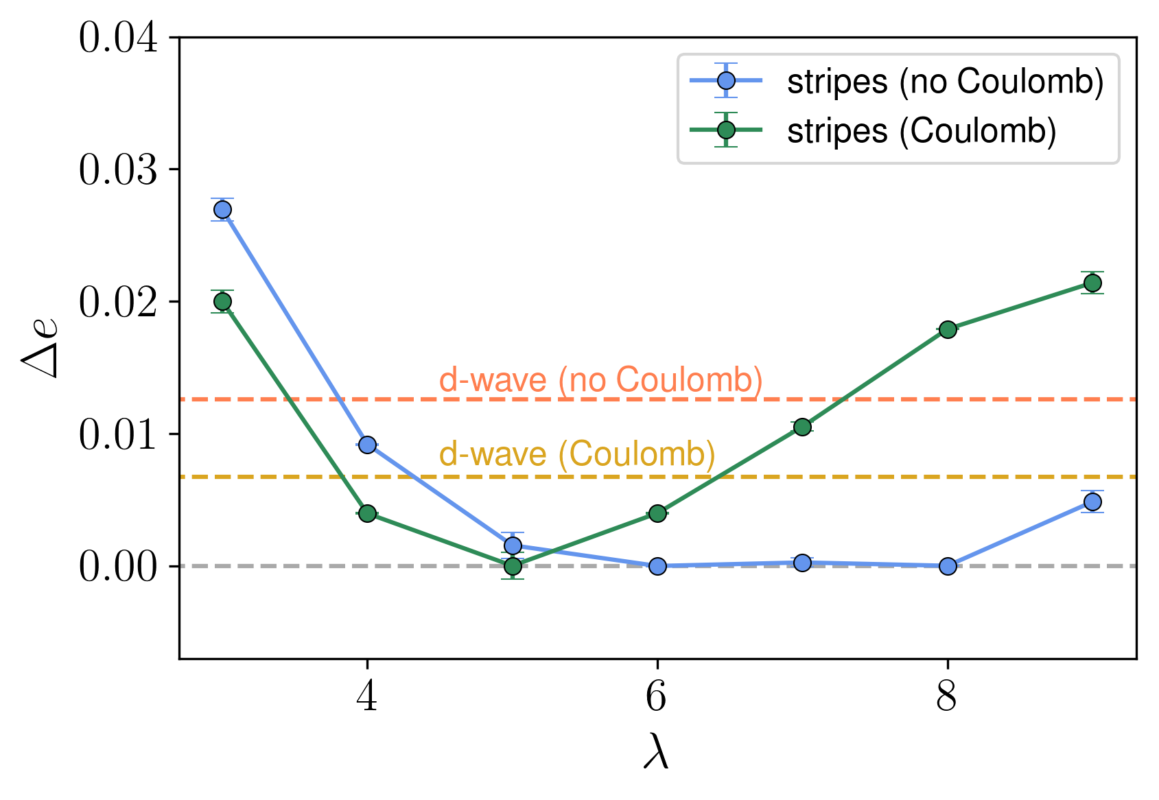
Figure 5.9: Energy landscape before and after adding the estimated long-range Coulomb interaction for vertical stripes of different wavelength. The charge distributions are from DMET calculations.

Another possibility is the long-range Coulomb repulsion. Long-range repulsion can play a dual role, in both driving charge inhomogeneity, as well as smoothing it out. In the Hubbard model, where stripes naturally form, the latter property can help drive the ground state towards shorter stripe wavelengths. In Fig. 5.9 we show the estimated effect of the long-range interactions on the stripe energetics by computing the Coulomb energy of the charge distributions of stripes with wavelengths $\lambda=3$–$9$. We use a dielectric constant of 15.5 (in the range proposed for the cuprate plane [249]). As shown in Fig. 5.9, the long-range Coulomb interaction favors shorter wavelength stripes and the homogeneous $d$-wave state, lifting the near-degeneracy of the stripes, shifting the ground state to $\sim 2/3$-filled stripe and making the uniform $d$-wave state also more competitive. Including the long-range Coulomb interaction favors the shorter wavelength stripes that is $\sim O(0.01t)$ per site for the $\lambda=4$ versus $\lambda=8$ stripe. Although this is only an order of magnitude estimate, it is on the same energy scale as the stripe energetics in Fig. 5.4, and thus provides a plausible competing mechanism for detailed stripe physics in real materials.

5.4 Conclusions

In summary, in this work we have employed state-of-the-art numerical methods to determine the ground state of the iconic $1/8$ doping point of the 2D Hubbard model at moderate to strong coupling. Through careful convergence of all the methods, and exhaustive cross checks and validations, we are able to eliminate several of the competing orders that have been proposed for the underdoped region in favor of a vertical striped order with wavelength near $\lambda\approx 8$. The striped order displays a remarkably low energy scale associated with its wavelength, which implies strong fluctuations either at low temperature or in the ground-state itself. This low energy scale can roughly be described at the mean-field level with a strongly renormalized $U$. We find coexisting pairing order with a strength intertwined with the stripe wavelength, indicating a coupling of stripe fluctuations to superconductivity. The stripe degeneracy is robust as the coupling strength is changed.

It has long been a goal of numerical simulations to provide definitive solutions of microscopic models. Our work demonstrates that even in one of the most difficult condensed matter models, such unambiguous simulations are now possible. In so far as the 2D Hubbard model is a realistic model of high-temperature superconductivity, the stripe physics observed here provides a firm basis for understanding the diversity of inhomogeneous orders seen in the materials, as well as a numerical foundation for the theory of fluctuations and its connections to superconductivity. However, our work also enables us to see limitations of the Hubbard model in understanding real HTSC’s. Unlike the stripes at this doping point in real materials, we find filled stripes rather than near half-filled stripes. Given the very small energy scales involved, terms beyond the Hubbard model, such as long-range Coulomb interactions, will likely play a role in the detailed energetics of stripe fillings. The work we have presented provides an optimistic perspective that achieving a comprehensive numerical characterization of more detailed models of the HTSC’s will also be within reach.

Appendix 5.A Appendix

5.A.1 Additional Information for the Figures and Discussion

Figure  5.2. The plotted energies (units of $t$) correspond to the following specific calculations.

• AFQMC: $-0.766\pm 0.001$ from extrapolation to $\infty$ (in both length and width directions) clusters with pinning fields.

• DMRG: $-0.7627\pm 0.0005$ from extrapolation to $\infty\times 6$ clusters with pinning fields using the hybrid momentum/real-space representation.

• DMET: $-0.77063\pm 0.00001$ from $8\times 2$ clusters with spin-inversion boundary conditions.

• iPEPS: $-0.7673\pm 0.002$ from $16\times 2$ supercells with extrapolation to zero truncation error.

Wavelengths of stripes. A key feature of the stripes is that each stripe acts as an antiferromagnetic domain wall. As a well-known consequence, at $1/8$ doping for half-filled stripes, the wavelength associated with the AF periodicity ($8$) is twice that of the charge periodicity ($4$). As an oversimplified but useful characterization of this periodicity, we describe it by labeling the spin pattern along a fixed row, assuming the stripe is width $1$: $\ldots\cdot\uparrow\downarrow\uparrow\cdot\downarrow\uparrow\downarrow\cdot\uparrow\downarrow\uparrow\cdot\ldots$. Here the $\cdot$’s indicate the positions of the localized hole, and the patterns $\uparrow\cdot\downarrow$ or $\downarrow\cdot\uparrow$ signify the domain wall nature of the stripe. Consider a charge wavelength which is an odd integer, e.g. $5$: $\ldots\cdot\uparrow\downarrow\uparrow\downarrow\cdot\uparrow\downarrow\uparrow\downarrow\ldots$ We see that the ratio of AF and charge wavelengths is one in this case, not two! This odd-even alternation is potentially confusing, particularly if one has non-integer charge periodicity.

However, experimentally, one looks at structure factors, noting peaks near $(\pi,\pi)$. The locations of the peaks nearest $(\pi,\pi)$ do not show any odd/even alternation. To see this note that the shift of the $k$-space origin to $(\pi,\pi)$, for one particular row, is equivalent to an alternating sign chain $-1^{x}$ in the AF pattern, e.g. for charge wavelength $4$,

$$\ldots\cdot\uparrow\downarrow\uparrow\cdot\downarrow\uparrow\downarrow\cdot\uparrow\downarrow\uparrow\cdot\ldots\to\ldots\cdot\uparrow\uparrow\uparrow\cdot\downarrow\downarrow\downarrow\cdot\uparrow\uparrow\uparrow\cdot\ldots$$

and for charge wavelength $5$

$$\ldots\cdot\uparrow\downarrow\uparrow\downarrow\cdot\uparrow\downarrow\uparrow\downarrow\ldots\to\ldots\cdot\uparrow\uparrow\uparrow\uparrow\cdot\downarrow\downarrow\downarrow\downarrow\ldots$$

In both the even and odd cases, the distance of peaks from $(\pi,\pi)$ corresponds to an AF “wavelength” of twice the charge wavelength.

5.A.2 Summary of Stripe Energy Results

Table 5.2: Best estimates of energies per site for stripes and and other low-energy state for $U/t=8$. For the AFQMC calculations (PBC) denotes periodic boundary conditions used on both the short- and long-axes of the cylinder. For the DMRG (real-space) calculations, periodic boundary conditions were used along the short axis, open boundary conditions on the long axis. For the hybrid basis DMRG (h-DMRG) calculations, periodic or anti-periodic boundary conditions were used on the short axis, denoted PBC or APBC. SF denotes that the DMET correlation potential in the spin-channel is flipped, doubling the spin wavelength. (Thus the $8\times 2$ (SF) pattern in DMET has a charge wavelength of 8 but a spin wavelength of 16.)

Method	Size	Wavelength	Energy ($t$)	Error ($t$)
AFQMC	$12\times 8$ (PBC)	$6$	$-0.7653$	0.0002
AFQMC	$14\times 8$ (PBC)	$7$	$-0.7653$	0.0002
AFQMC	$16\times 8$ (PBC)	$8$	$-0.7668$	0.0002
AFQMC	$18\times 8$ (PBC)	$9$	$-0.7655$	0.0002
AFQMC	$20\times 8$ (PBC)	$10$	$-0.7653$	0.0002
AFQMC	$\infty\times 4$	$8$	$-0.7680$	0.0001
AFQMC	$\infty\times 6$	$8$	$-0.7653$	0.0003
AFQMC	$\infty\times 8$	$8$	$-0.7656$	0.0004
DMRG	$\infty\times 4$	$8$	$-0.76598$	0.00003
DMRG	$\infty\times 6$	$5$	$-0.7615$	0.0004
DMRG	$\infty\times 6$	$8$	$-0.762$	0.001
DMRG	$\infty\times 7$	$7$	$-0.762$	0.001
DMRG	$\infty\times 6$	$9$	$-0.751$	0.0016
h-DMRG	$\infty\times 6$ (PBC)	$5$	$-0.76210$	0.00005
h-DMRG	$\infty\times 4$ (APBC)	$8$	$-0.76057$	0.00007
h-DMRG	$\infty\times 4$ (PBC)	$8$	$-0.7657$	0.0003
h-DMRG	$\infty\times 4$ (av.)	$8$	$-0.7631$	0.0003
h-DMRG	$\infty\times 6$ (PBC)	$8$	$-0.7627$	0.0005
DMET	$2\times 2$	$d$-wave	$-0.7580$	$0.0005$
DMET	$3\times 2$	$3$	$-0.7437$	$0.0009$
DMET	$4\times 2$ (SF)	$4$	$-0.7614$	$0.00005$
DMET	$5\times 2$	$5$	$-0.7691$	$0.001$
DMET	$6\times 2$ (SF)	$6$	$-0.7706$	$0.00007$
DMET	$7\times 2$	$7$	$-0.7704$	$0.0003$
DMET	$8\times 2$ (SF)	$8$	$-0.7706$	$0.00001$
DMET	$9\times 2$	$9$	$-0.7658$	$0.0008$
DMET	$2\sqrt{2}\times\sqrt{2}$	$d$-wave	$-0.7620$	$0.00001$
DMET	$5\sqrt{2}\times\sqrt{2}$	frustrated	$-0.7689$	$0.0008$
iPEPS	$2\times 2$	$2$	$-0.7560$	$0.0025$
iPEPS	$5\times 2$	$5$	$-0.7632$	$0.0018$
iPEPS	$7\times 2$	$7$	$-0.7629$	$0.0026$
iPEPS	$16\times 2$	$8$	$-0.7673$	$0.002$
iPEPS	$16\times 16$	diag. $4\sqrt{2}$	$-0.7581$	$0.0014$

Table 5.3: Best estimates of energies per site for stripes and other low-energy states for $U/t=6$.

Method	Size	Wavelength	Energy ($t$)	Error ($t$)
AFQMC	$12\times 8$ (PBC)	$6$	$-0.8684$	0.0001
AFQMC	$14\times 8$ (PBC)	$7$	$-0.8692$	0.0001
AFQMC	$16\times 8$ (PBC)	$8$	$-0.8718$	0.0001
AFQMC	$18\times 8$ (PBC)	$9$	$-0.8701$	0.0001
AFQMC	$20\times 8$ (PBC)	$10$	$-0.8702$	0.0001
DMET	$2\times 2$	$d$-wave	$-0.8679$	$0.0007$
DMET	$3\times 2$	$3$	$-0.85867$	$0.00004$
DMET	$4\times 2$	$4$	$-0.85890$	$0.00004$
DMET	$5\times 2$	$5$	$-0.86836$	$0.00001$
DMET	$6\times 2$ (SF)	$6$	$-0.87247$	$0.00001$
DMET	$7\times 2$	$7$	$-0.87363$	$0.00002$
DMET	$8\times 2$ (SF)	$8$	$-0.87667$	$0.0007$

Table 5.4: Best estimates of energies per site for stripes and other low-energy states for $U/t=12$.

Method	Size	Wavelength	Energy ($t$)	Error ($t$)
AFQMC	$10\times 8$ (TABC)	$5$	$-0.6446$	0.0006
AFQMC	$12\times 8$ (TABC)	$6$	$-0.6452$	0.0004
AFQMC	$14\times 8$ (TABC)	$7$	$-0.6461$	0.0006
AFQMC	$16\times 8$ (TABC)	$8$	$-0.6458$	0.0006
AFQMC	$18\times 8$ (TABC)	$9$	$-0.6462$	0.0006
AFQMC	$20\times 8$ (TABC)	$10$	$-0.6450$	0.0006
DMRG	$\infty\times 4$	4	-0.641379	0.000052
DMRG	$\infty\times 4$	5	-0.64269	0.00019
DMRG	$\infty\times 4$	6	-0.64285	0.00021
DMRG	$\infty\times 4$	8	−0.64168	0.00023
DMRG	$\infty\times 6$	4	-0.6383	0.0026
DMRG	$\infty\times 6$	5	-0.64148	0.00059
DMRG	$\infty\times 6$	6	-0.6418	0.0013
DMRG	$\infty\times 6$	8	-0.6438	0.0019
DMET	$2\times 2$	$d$-wave	$-0.63940$	$0.00001$
DMET	$4\times 2$ (SF)	$4$	$-0.6505$	$0.0001$
DMET	$5\times 2$	$5$	$-0.6531$	$0.0001$
DMET	$6\times 2$ (SF)	$6$	$-0.6526$	$0.0002$
DMET	$8\times 2$ (SF)	$8$	$-0.6514$	$0.0001$

Chapter 6 More Realistic Models of High-T_c Superconductors 

6.1 Introduction

As discussed in Chapter 4 and 5, numerical studies of the one-band Hubbard model have achieved substantial progress regarding the ground state energies and orders, as well as various low-lying competing states even, even in the most difficult part of the phase diagram. This is possible only through combing various state-of-the-art approximate numerical methods to explore many candidate states proposed by theorists or discovered by previous computational and experimental studies. A great success as it is, the question arises that how relevant the results, or the one-band Hubbard model itself, are to the cuprates physics. As we discussed, the fact that many of the candidate states are in a small energy range in the 2D Hubbard model reflects an artificial degeneracy in this model. Any of these states could become the true ground state if the parameters are slightly varied to favor that state. Thus, to answer questions in experiments and to understand the factors that determine the superconductivity transition temperature, one has to go beyond the one-band Hubbard model and consider more details of the real materials.

In this chapter, we describe the applications of DMET to two more sophisticated systems: the three-band Hubbard model and a downfolded ab initio cuprate Hamiltonian. These models introduce multi-orbital and dynamical correlation effects, which could be important factors in real materials. Other interactions, such as long-range Coulomb interactions and interlayer coupling are not studied here, but could also have significant impact on the ground state and low-temperature behaviors of cuprate superconductors.

In Sec. 6.2, we discuss the background and results of the three-band Hubbard model. Sec. 6.3 describes the downfolded cuprate Hamiltonian and the DMET calculations on the system. We present the main conclusions in Sec. 6.4.

6.2 The Three-Band Hubbard Model

The model. The three-band Hubbard model simulates the physics of the CuO₂ plane of cuprates with the valence orbitals: the copper $d_{x^{2}-y^{2}}$ orbital and the oxygen bridge $p_{x}$ or $p_{y}$ orbitals [Fig. 6.1]. When undoped, there are 5 electrons in each unit cell, formally filling up the $p$ sites while the $d$ site is half filled. Physically, however, it forms an antiferromagnetic charge-transfer insulator, with occupation higher than one on the $d$ sites. Unlike the one-band Hubbard model, the three-band model has significant particle-hole asymmetry as the doped holes go primarily on the $p$ sites while the doped electrons reside on the Cu $d$ sites.

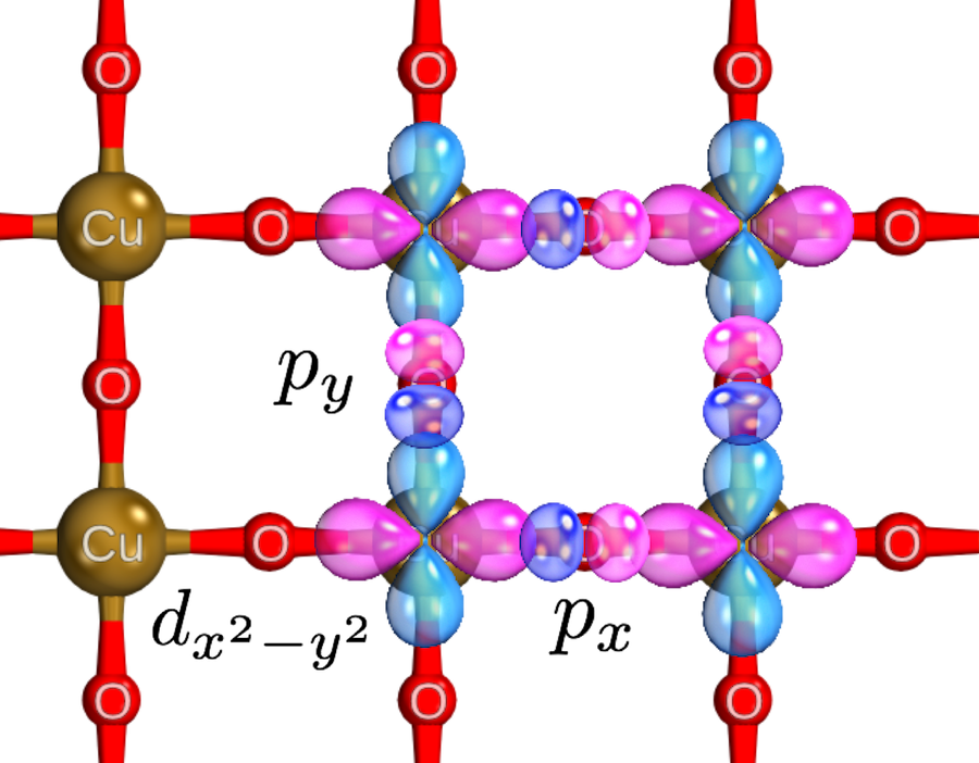
Figure 6.1: (a) The cuprate CuO₂ plane and the orbital arrangement of the three-band Hubbard model. (b) The common parameters in the three-band Hubbard model.

Previous numerical studies of the three-band model ground state using Lanczos, quantum Monte Carlo, dynamical mean-field theory, variational cluster approximation and diagrammatic perturbation show even richer charge, spin and pairing orders than in the one-band model [68, 259, 260, 261, 262, 263, 264, 265, 266]. Yet, because the model is numerically more difficult, fewer studies are carried out compared to the one-band Hubbard model. The numerical studies are far from reaching the thermodynamic limit (TDL) or having enough energy resolution to determine the ground state, especially in the dope model. DMET is thus a unique method that has the potential to carry out definitive numerical simulations on the three-band model with an affordable computational cost.

Computational details. The full parameterization of the three-band model usually includes the hopping between the nearest $d$ and $p$ orbitals $t_{pd}$, and between the nearest and next-nearest $p$-orbitals $t_{pp}$ and $t_{pp}^{\prime}$, onsite interactions $U_{d}$ and $U_{p}$, nonlocal Coulomb interaction $V_{pd}$ and the energy difference $\Delta=\varepsilon_{d}-\varepsilon_{p}$ [Fig. 6.1]. There are different approaches to map cuprates to the three-band model, thus a wide range of parameters are published and used in numerical studies, which do not always agree with each other  [267, 268, 269, 270, 271, 272, 262]. In our DMET calculations, we choose to use only the minimal set of parameters $U_{d}$, $t_{pd}$ and $\Delta$, from the common parameter sets summarized in Table 6.1. Note that we use the electron representation, which is different from literature conventions, where the parameters are written down for the holes.

Table 6.1: Model parameters used in this study, in unit of eV.

Source	$\mathbf{U_{d}}$	$\mathbf{t_{pd}}$	$\mathbf{\Delta}$
Hybertsen (1989) [269]	10.5	1.3	-6.9
Martin (1996) [272]	16.5	1.8	-11.1
Hanke (2009) [262]	12	1.5	-7.5

Figure 6.2: The 12-site fragment used in DMET studies of the three-band Hubbard model.

We carried out broken particle-number symmetry DMET calculations (see Appendix Sec. B.2) on the three-band model using fragments of 12 sites, on an auxiliary lattice of $20\times 20$ unit cells. In the three-band model, the conventional $2\times 2$ supercell breaks inversion symmetry and, since the Cu and O atoms become inequivalent in the impurity model, the symmetry would also break in the correlated wavefunction, leading to unfavored artifacts. To reduce this effect as much as possible, we follow Ref. [263] and use a modified $2\times 2$ cell which restores the inversion symmetry (Fig. 6.2). We varied occupations in the model and computed the energies, magnetic and pairing order parameters. Since it is not clear how to decompose the pairing order in the symmetry-broken three-band fragments, we use the total norm of local pairing order parameters as a proxy for the pairing order strength, which reflects the combined pairing strength in all symmetry sectors.

Results – undoped. The results for the undoped three-band model are summarized in Table 6.2. We find the charge transfer between the oxygen $p$-orbitals and the copper $d$ orbitals, and antiferromagnetic order with staggered magnetization $m\sim 0.37$, localized on $d$ orbitals. These results are consistent among all sets of parameters, and with previous studies  [68]. We also notice the more recent parameters from Martin (1996) and Hanke (2009) are more consistent with each other than Hybertsen (1989), indicating increasing consensus on the parameters of the model.

Table 6.2: Charge and staggered magnetization from 12-site DMET calculations on the three-band model.

Model	$\mathbf{n_{d}}$	$\mathbf{n_{p}}$	$\mathbf{m_{d}}$	$\mathbf{m_{p}}$
Hybertsen	1.237	1.882	0.363	0.000
Martin	1.218	1.891	0.377	0.000
Hanke	1.218	1.891	0.374	0.001

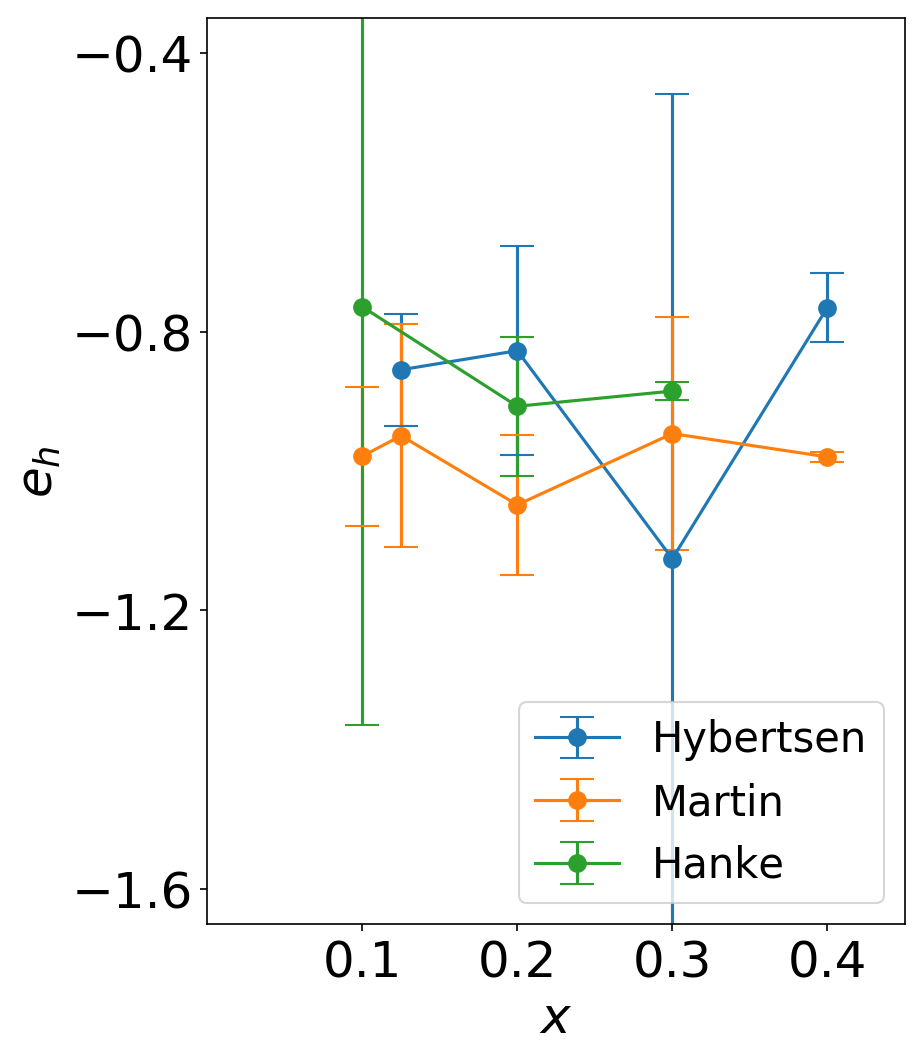
(a) hole energy

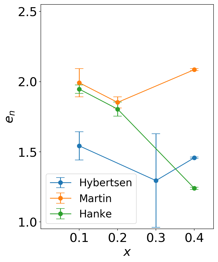
(b) electron energy

Figure 6.3: Energies per hole (electron) in hole (electron) doped three-band model for all three sets of parameters, in the unit of eV.

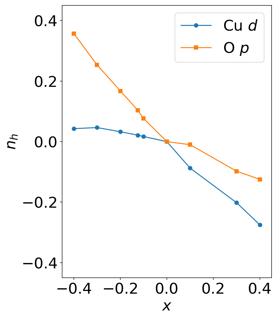
(a) Hybertsen

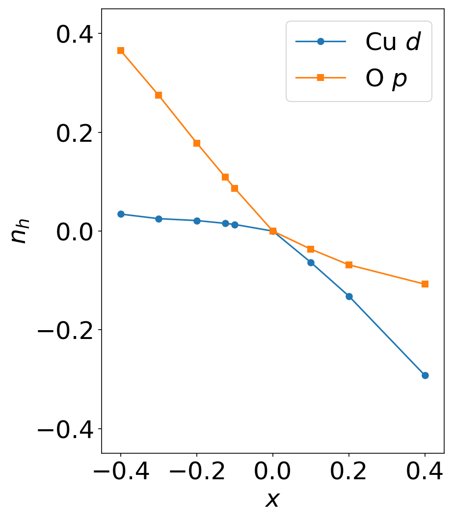
(b) Martin

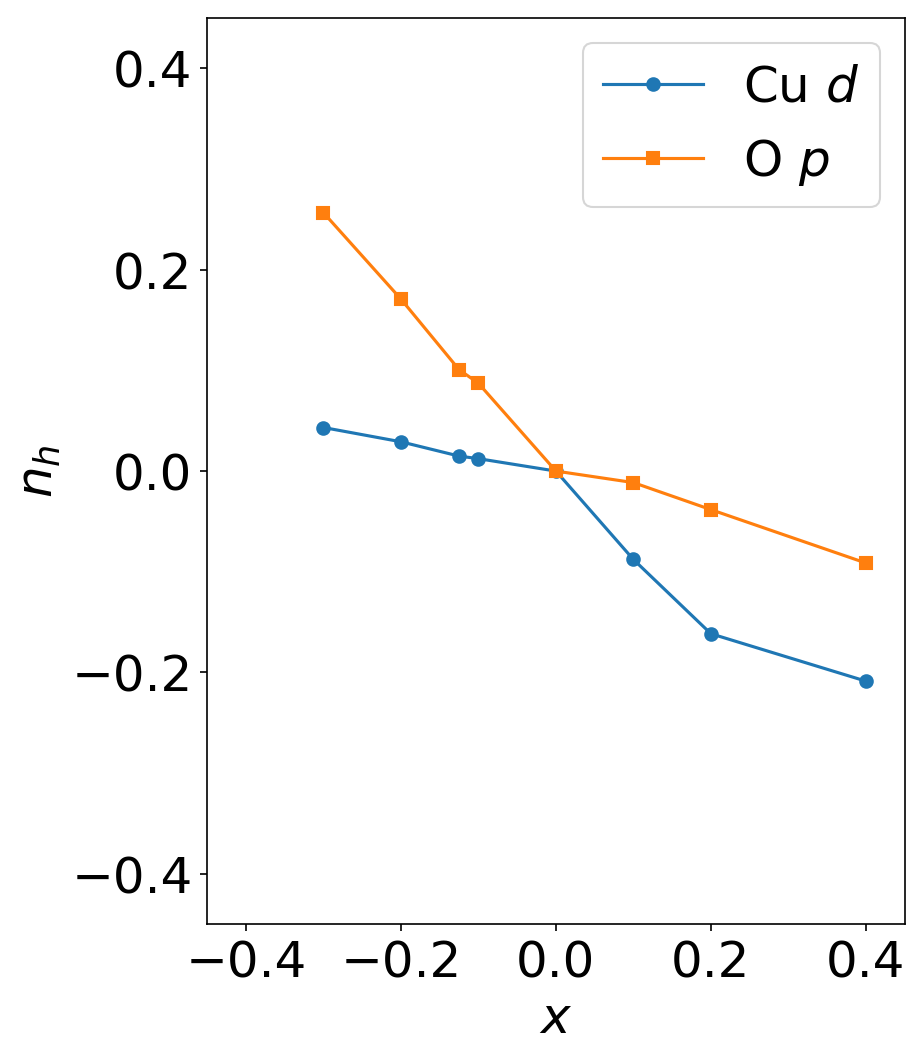
(c) Hanke

Figure 6.4: Hole distribution between $d$ and $p$ orbitals in the doped three-band model. The horizontal axis is doping where negative numbers indicate hole doping while positive numbers are electron doping. The hole distribution for $p$-orbitals is the sum of the two $p$-orbitals in a unit cell.

Results – energy and charge distribution. We plot the energies per hole and energies per electron for the doped three-band model in Fig. 6.3. Since we do not perform fragment size extrapolation, the error bars only show the DMET convergence errors. We notice on both hole- and electron-doped sides, there are points with large error bars. These reflect either DMET has experienced convergence issues, or the energy becomes sensitive to small changes in the correlation potential, usually because the correlation potential has redundant or unnecessary degrees of freedom. Thus, it is necessary to explore better parameterization of $u$ to avoid this problem.

Nevertheless, Fig. 6.3 is still informative. For hole-doped cuprates, the energies per hole are almost constant (between $-1.2$eV and $-0.8$eV) when doping is varied in all the parameters, suggesting the phase separation or inhomogeneous orders are likely to appear for a wide range of doping. On the electron doped side, the energies per (doped) electron have different behaviors for the parameters we use: Martin and Hybertsen are more or less constant around $2.0$eV and $1.5$eV, respectively, while Hanke gives decreasing energy per electron, leading to strong phase separation effect. These unusual and inconsistent behaviors reflect that these models do not correctly describe the electron-doped cuprates, simply because they are fitted to the hole-carrier superconductors, such as La_2-xSr_xCuO₄.

In Fig. 6.4, we summarize the charge distribution when the model is doped for all three sets of parameters. The numbers are averaged over local charge distributions. As expected, when the system is hole-doped, the holes go primarily to the oxygen $p$ sites, while the doped electrons tend to stay on the copper $d$ sites. This leads to the particle-hole asymmetry in cuprate superconductors, and is correctly described by the three-band model using DMET.

Results – spin and pairing orders. In Fig. 6.5, we show the antiferromagnetic (AF) and pairing order parameters in the hole-doped three-band model. We do not display the electron-doped side because from what we learned before, the parameters we use do not seem to describe the correct physics on the electron-doped side. The magnetic order parameters are averaged over the copper $d$ sites with the $(\pi,\pi)$ structure factor, as there is virtually no spin on the $p$ orbitals when the model is doped. Overall, the shapes of the order parameter curves and sizes are similar to what we obtained from one-band model calculations.

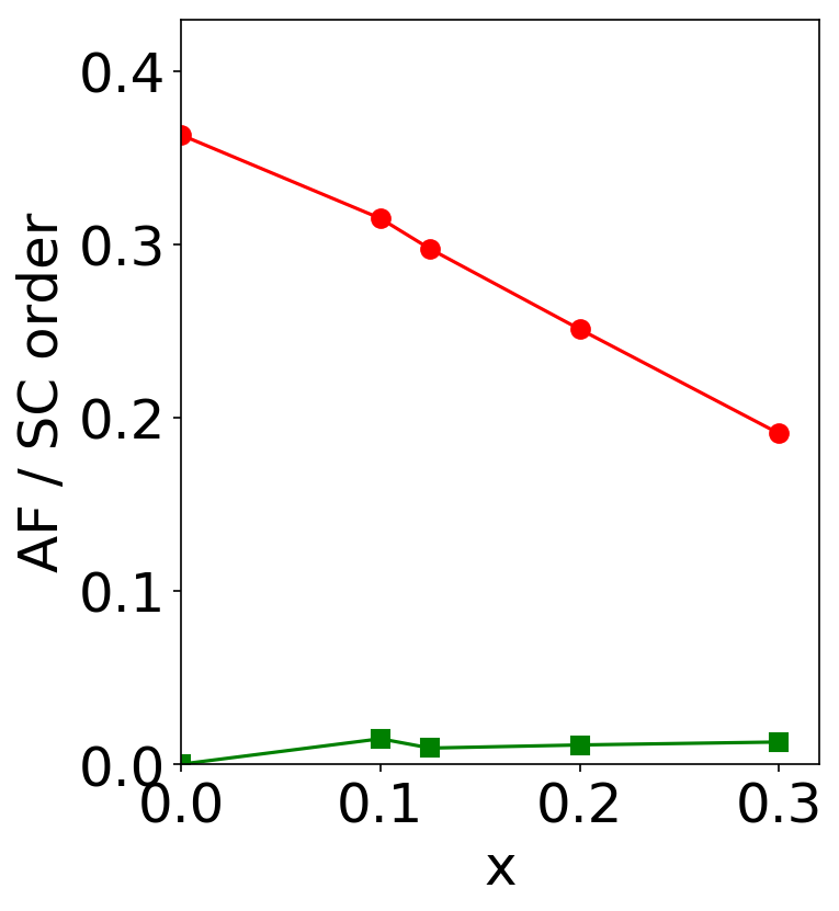
(a) Hybertsen

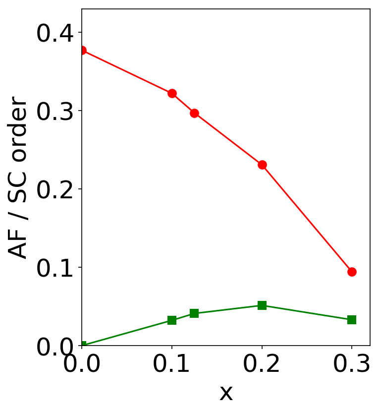
(b) Martin

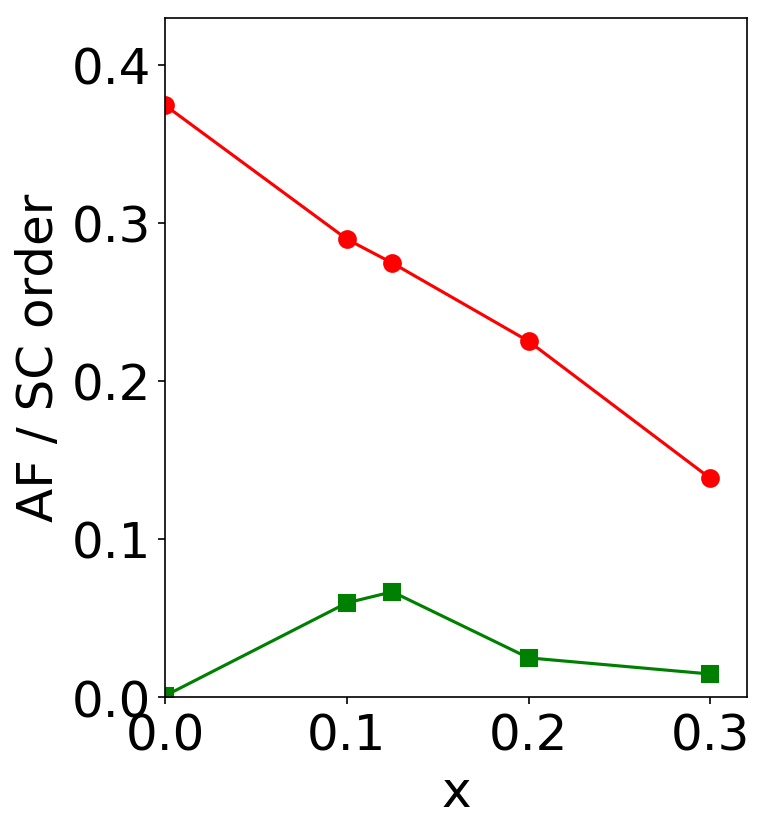
(c) Hanke

Figure 6.5: Averaged antiferromagnetic (red circle) and total pairing (green square) order parameters in the hole-doped three-band model for all sets of parameters from DMET.

The AF order decreases with increasing doping, consistent with what we find in the one-band Hubbard model and cuprates. The order remains robust at $x=0.3$ doping, with the value $\sim 0.1$–$0.2$, which is probably overestimated. It is a known issue in DMET to overestimate magnetic order parameters in small fragments, which can be eliminated by increasing the fragment size and extrapolating to the TDL. Both results from Martin and Hanke show a superconducting dome (in terms of the magnitudes of the order parameters, rather than transition temperature), with maximum pairing at $x=0.2$ and $x=0.125$, respectively. This is plausible behavior one would expect from the experience. The Hybertsen parameters, however, give virtually no pairing order in the whole parameter range.

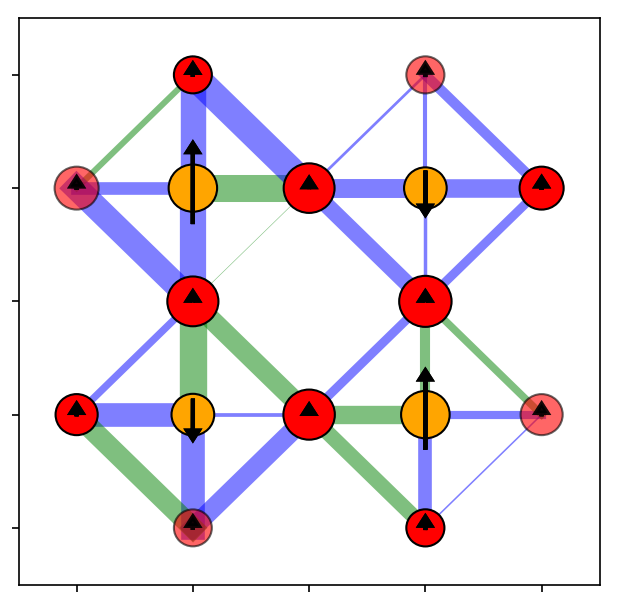
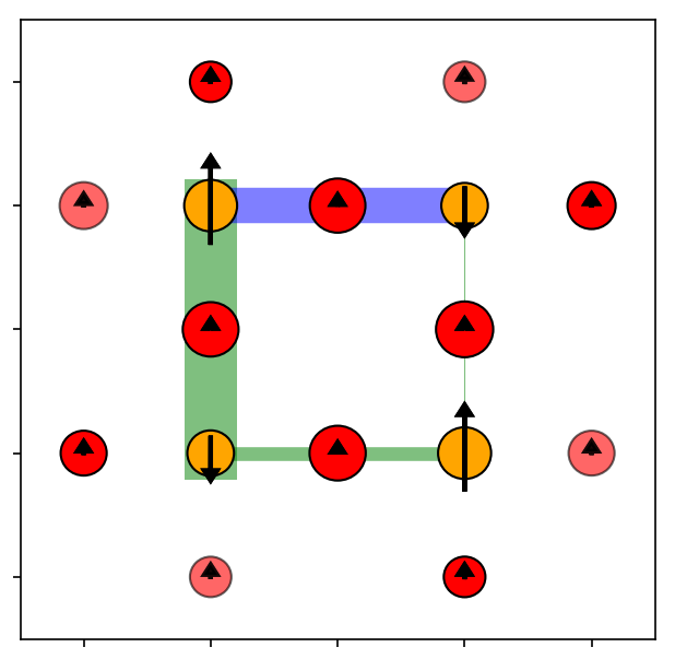
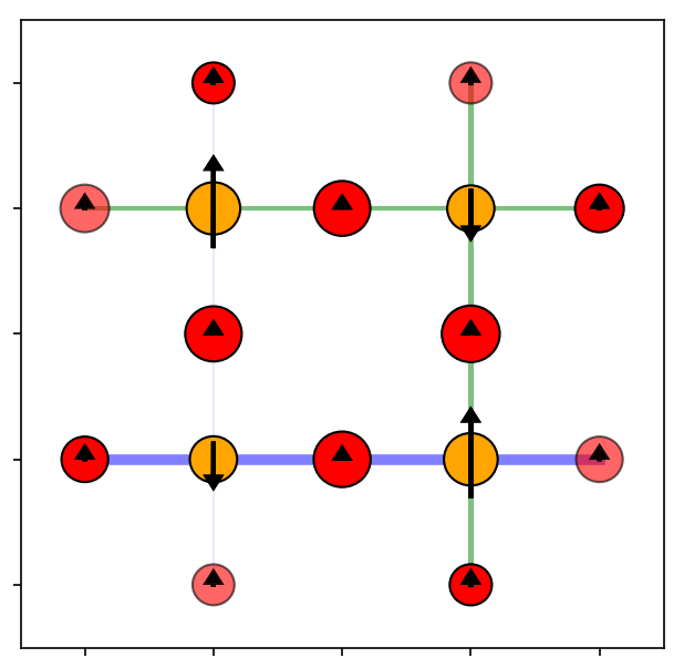
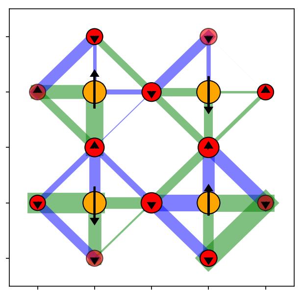
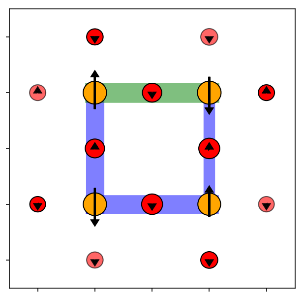
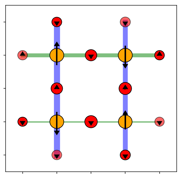
Figure 6.6: Charge, spin and pairing patterns of the three-band model. The diameters of the red circles are proportional to the hole densities, the sizes of the arrows are proportional to staggered magnetization, and the width of the ribbons are proportional to pairing strength. (a) to (c) show parameters from Martin, with $x=0.2$ doping. (d) to (f) show parameters from Hanke, with $x=0.125$ doping. (a) and (d) show nearest neighbor pairings; (b) and (e) show pairings between Cu $d$-orbitals; (c) and (f) show pairings between next-nearest-neighbor O $p$-orbitals.

Fig. 6.6 shows the local orders at the optimal doping points using parameters from Martin and Hanke. The charge and spin orders do not show much inhomogeneity, while the pairing order is much more complicated than the simple $d$-wave symmetry we saw in the one-band model. Overall, the pairing strength is strongest between neighboring sites (including nearest $p$ orbitals) and between $d$ orbitals. Besides the most common $d_{x^{2}-y^{2}}$ symmetry, we can also recognize extended $s$-wave (eg., between nearest $p$ sites), $p$-wave and $d_{xy}$-wave pairing. However, it is not clear enough how to decompose the real space pairings into angular momentum sectors (coupled with spatial inhomogeneity) for the DMET results. It is unlikely that the pairing irregularity is an artifact, because the spin and charge orders seem reasonable, and the trends for the total pairing strength are also as expected.

Conclusions. We conducted an exploratory investigation of the three-band model using DMET using a 12-site symmetrized fragment. Using the conventional DMET algorithms designed for the one-band model, we were not able to control the energy accuracy to similar magnitudes, mainly due to the difficulties in converging the DMET energies. Nevertheless, we obtain reasonable charge and spin distributions for the undoped and hole-doped models with all the parameters we examed, while the local pairing order parameters show complicated spatial and angular momentum distribution, which requires further investigations with higher energy accuracy to confirm or reject. Other future directions include employing impurity solvers which are more scalable such as CASSCF solvers, to study larger fragments on inhomogeneity and to extrapolate to the TDL.

6.3 Realistic Cuprates from Hamiltonian Downfolding

The Hamiltonian and computational strategy. The ultimate goal in material numerical studies is being able to compute properties of strongly correlated materials from first principles. To do this, one has to go beyond model systems and form a streamlined approach to process real materials similar to DFT for normal materials. DMFT+DFT has been a very successful practice and applied to many important problems so far (See, eg., Refs. [45, 273, 274, 275]). However, despite the huge computational cost, DMFT also suffers from the so-called double counting problem [276], where the correlation energy is included in both DMFT and DFT calculations. To fix the double counting problem, one usually has to introduce system-dependent terms derived from experience or experimental data.

In addition to exploring a parameter-free treatment of cuprates, we would also like to find an alternative path to study general strongly correlated materials from first principles using DMET. We propose the following algorithm to carry out the calculations:

1. Compute the band structure using DFT or Hartree-Fock, and use the information to construct, in a local basis, the Fock matrix of the lattice system, the local one-body density matrix and the local two-body integrals.

2. Project the local one-body density matrix to each atom and form the atomic natural orbitals (ANO). Choose relevant ANOs to form the basis of the correlated calculations. Remove the Coulomb and exchange contributions from the correlated ANOs in the lattice Fock matrix.

3. Perform DMET calculations based on the effective hopping (lattice Fock matrix minus contributions from correlated ANOs) and local two-body integrals (in the ANO basis).

4. Once DMET is converged, add the correlation potential $u$ to the DFT or Hartree-Fock calculations in step 1, and perform the calculations in step 1 to 3 again, until convergence.

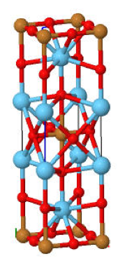
(a) La₂CuO₄

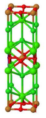
(b) Ca₂CuO₂Cl₂

Figure 6.7: Conventional cells of cuprate superconductors La₂CuO₄ and Ca₂CuO₂Cl₂. For La₂CuO₄, we use a cubic structure without John-Teller distortion.

In this work, we carried out small proof-of-principle calculations on La₂CuO₄ and Ca₂CuO₂Cl₂, whose structures are shown in Fig. 6.7. For step 1, we performed the spin-restricted DFT calculations with the periodic Gaussian double-zeta basis fitted as linear combinations of plane wave functions, detailed in Ref. [277]. Lately, new periodic DFT / Hartree-Fock codes are available and would presumably be more efficient and robust to use [278]. For step 2, we project the one-body density matrix to atomic basis by taking the corresponding blocks of the density matrix, and diagonalize them to obtain the ANOs. Alternatively, we could take the corresponding rows and run SVD to obtain a slightly different set of ANOs. The ANOs we obtained show clear characteristics of orbital shape and occupation. In Fig. 6.8 we plot the projected density of states to the full CuO₂ plane and to the ANO space. By including $\sim 26$ orbitals per unit cell, it is already sufficient to reproduce the PDOS near the Fermi level (up to $\sim 3$eV above), and serves as a realistic correlation model for the real material. Thus, if we choose the $2\times 2$ supercell as the fragment, the total number of orbitals is around 100 per fragment, or 200 per impurity model, most of which are weakly correlated. Thus, it is possible to use CASSCF impurity solvers coupled with DMRG to treat the impurity models.

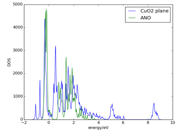
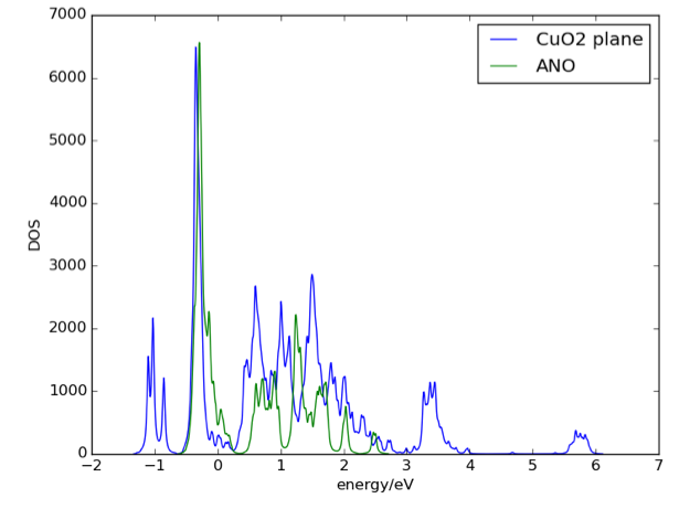
Figure 6.8: Projected density of states (DOS) for the CuO₂ plane from original DFT band structure and projected ANO one-body density matrices. (a) La₂CuO₄ with Cu $3d,4s,4p,4d,5s$ and O $2p,3p$ orbitals (27 orbitals per unit cell); (b) Ca₂CuO₂Cl₂ with Cu $3d,4s,4p,4d$ and O $2p,3p$ orbitals (26 orbitals per unit cell).

To illustrate the principle, however, we further freeze most of the ANOs but 5 per unit cell: Cu $3d_{x^{2}-y^{2}},4s,4d_{x^{2}-y^{2}}$ and O $2p_{x/y}$ orbitals. Although the impurity model is now small enough to be solved with DMRG alone, we instead use the DMRG/CASSCF solver with 12 active orbitals. The calculations are carried out without broken particle-number symmetry and we did not perform the macro self-consitency between the DFT and DMET calculations (step 4).

Results. In the undoped material, the average occupations on Cu atoms (the three orbitals) are 1.832 and 2.012 for La₂CuO₄ and Ca₂CuO₂Cl₂, respectively. This seems unreasonable but may merely reflect the renormalization between $p$-orbitals and virtual orbitals on Cu. Besides, since we include two virtual orbitals on each Cu atom but no virtual orbitals on O atoms, there may be an imbalance between the two species that drives the artificial charge transfer. If we only look at the Cu $3d_{x^{2}-y^{2}}$ orbital, the occupations are 1.382 and 1.410.

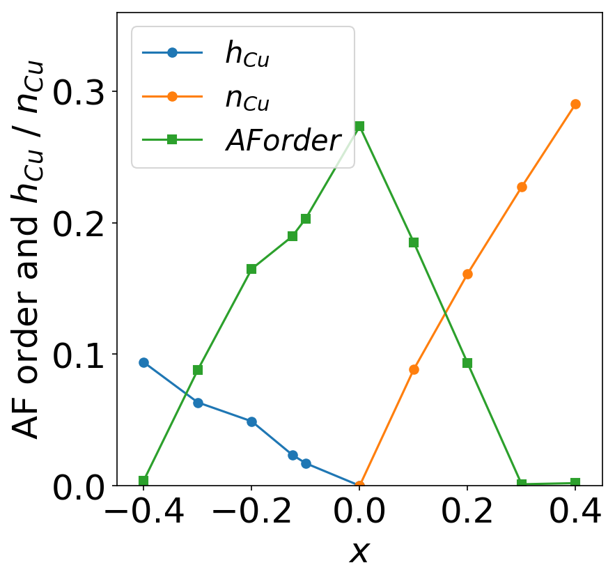
(a) La₂CuO₄

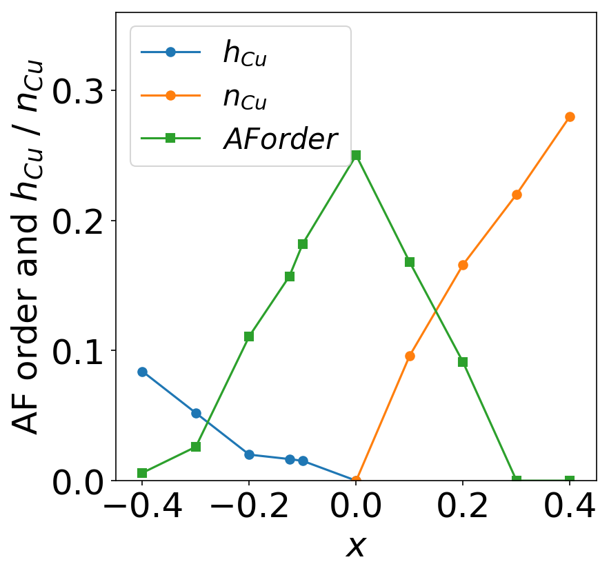
(b) Ca₂CuO₂Cl₂

Figure 6.9: Averaged antiferromagnetic order parameters and hole/electron densities on Cu atoms for various doping levels in cuprates, from 5-band DMET calculations. Positive $x$ means electron doping, while negative $x$ means hole doping.

Fig. 6.9 shows the hole/electron densities on copper and the AF order, versus doping. When $x=0$, i.e., undoped, the AF order is slightly higher in La₂CuO₄ ($m=0.273$) than in Ca₂CuO₂Cl₂ ($m=0.250$). These numbers are smaller than experimental values, but the order is consistent: the Néel temperature for La₂CuO₄ is around 300K, compared to $\sim$250K for Ca₂CuO₂Cl₂ [279, 280]. The quantitative disagreement may be due to the spin-restricted Fock matrix from DFT calculations, which suppresses the magnetic order. This could be fixed by introducing the self-consistency between DFT and DMET. When the cuprates are doped, the holes go primarily to oxygen $p$ orbitals while electrons mostly go to copper $d$ orbitals, consistent with our results on the three-band model. Thus, the AF order is destroyed faster on the electron-doped side compared to hole-doped side. This is opposite to what happens in the generic cuprate phase diagram, and not what one would expect. However, by inspecting the results more carefully, we find signs of broken spatial symmetry and development of inhomogeneous orders in the underdoped region of the hole-doped cuprates, which is much weaker for electron-doped cuprates. Thus, once we go to larger fragments, the inhomogeneous orders may be stabilized and destroy the AF order in the hole-doped cuprates; while the AF order survives for electron doping. This conjecture is consistent with what we saw in the 1D Hubbard model calculations, as well as the results here, and seems a plausible explanation for the particle-hole asymmetry in the generic cuprate phase diagram. Confirming this conjecture may require larger fragments similar to those used in the one-band Hubbard model studies.

Conclusions. We demonstrate a DFT/HF-DMET approach to study strongly correlated materials from first principles without any artificial parameters. The approximations involved in these calculations are by no means converged or controlled. However, we achieve qualitatively correct results in all respects we have access to. With an improved treatment in all the steps involved, it is promising to finally perform accurate calculations of cuprates from first principles.

6.4 Conclusions

We present two exploratory applications of DMET to study the cuprate physics beyond the one-band Hubbard model. General qualitative features, such as the interplay of antiferromagnetic and pairing orders, instabilities to inhomogeneous phases, remain in these systems, while to reach the quantitative details requires more effort to improve the DMET algorithm. With further developments in the method, impurity solvers and computational resources, ab initio, predictive calculations of high-T_c superconductivity in cuprates is an achievable goal.

Chapter 7 Finite Temperature Density Matrix Embedding Theory: A Superoperator Approach 

7.1 Introduction

While ground state wavefunctions contain rich information about the materials, it is still desirable to access finite-temperature properties, partly because most experimental measurements happen in finite temperature and it is easy to obtain the temperature dependence of physical observables.

Thus, extending DMET to finite temperature would significantly expand the scope of the method, which becomes potentially useful for studying chemical dynamics, spectral properties and directly observe superconducting phase transition in cuprates.

A simple “hack” to enable finite temperature calculations is to use the thermal one-body density matrix to replace the ground-state density matrix in DMET, and finite-temperature impurity solvers to replace ground state solvers. A problem of this approach is that the one-body density matrix is no longer idempotent, and the number of bath orbitals is not bounded anymore; although we can always truncate the bath orbitals, it becomes increasingly hard to do so at high temperature. The more serious issue is that, this approach does not have a solid theoretical framework to guarantee its correctness. Nevertheless, this approach is of low cost and minimal implementation effort and thus is worth exploring for low-temperature applications.

In this chapter, however, we discuss another approach based on the singular value decomposition (SVD) of the density operator, analogous to the SVD of the wavefunction in the ground-state formulation. The central problem here, is how to define a Hilbert space for the mean-field density operators, which enables SVD in the single-particle basis, similar to the Schmidt decomposition of mean-field wavefunctions. It turns out that a mathematical tool called superoperators can be applied to solve this problem. In Sec. 7.2, we introduce the theoretical framework in detail. Then we present the conclusions in Sec. 7.3.

7.2 Theory

7.2.1 The Superoperator Space

The superoperator formalism provides a way to encode thermal density operators as vectors in a fermion Fock space, thus one can perform operations such as creation, annihilating, inner product, etc. similar to wavefunctions.

To derive the formulation, we use the spinless notation for simplicity. We start by writing the normal fermion creation (annihilation) operators as Majorana fermions (we reserve $i$ as the complex number unit)

$$w_{2j-1}=a_{j}+a_{j}^{\dagger}\ \ w_{2j}=i(a_{j}-a_{j}^{\dagger}).$$ (7.1)

The Majorana fermions are the antiparticles of themselves, thus $w_{k}w_{k}=1$ (this can also be derived rigorously using Eq. 7.1). For any operator $\hat{O}$ as finite or infinite polynomial expansions of $\{a_{j}^{(\dagger)}\}$, the Majorana transformation leads to a linear combination of Majorana fermion strings

$$w_{1}^{\alpha_{1}}w_{2}^{\alpha_{2}}\dots w_{2n}^{\alpha_{2n}}$$

where $\alpha_{i}=0$ or $1$. Thus, each of the $2^{n}$ string in the Majorana fermion string space can be written as a string of $\{\alpha_{i}\}$, and

$$\hat{O}=\sum_{\alpha_{1},\ldots,\alpha_{2n}}C_{\alpha_{1}\ldots\alpha_{2n}}w_{1}^{\alpha_{1}}w_{2}^{\alpha_{2}}\dots w_{2n}^{\alpha_{2n}}=\sum_{\alpha_{1},\ldots,\alpha_{2n}}C_{\alpha_{1}\ldots\alpha_{2n}}|\alpha_{1}\cdots\alpha_{2n}).$$ (7.2)

We can define creation and annihilation operators in the superoperator space

$$f_{k}|O)=\alpha_{k}|w_{k}O)\ \ \ \ \ f_{k}^{\dagger}|O)=(1-\alpha_{k})|w_{k}O)$$ (7.3)

where $|w_{k},\alpha_{1},\cdots,\alpha_{k},\cdots,\alpha_{2n})=(-1)^{\alpha_{1}+\ldots+\alpha_{k-1}}|\alpha_{1},\cdots,1-\alpha_{k},\cdots,\alpha_{2n})$. We can easily compute the anticommutation relations

$$\begin{split}\{f_{k},f_{l}\}|O)=&\alpha_{k}\alpha_{l}[|w_{k}w_{l}O)+|w_{l}w_{k}O)]\delta_{k\neq l}\\ &+2(1-\alpha_{k})\alpha_{k}|O)\delta_{k=l}=0\\ \{f_{k}^{\dagger},f_{l}^{\dagger}\}|O)=&(1-\alpha_{k})(1-\alpha_{l})[|w_{k}w_{l}O)+|w_{l}w_{k}O)]\delta_{k\neq l}\\ &+2(1-\alpha_{k})\alpha_{k}|O)\delta_{k=l}=0\\ \{f_{k}^{\dagger},f_{l}\}|O)=&(1-\alpha_{k})\alpha_{l}[|w_{k}w_{l}O)+|w_{l}w_{k}O)]\delta_{k\neq l}\\ &+[(1-\alpha_{k})^{2}+\alpha_{k}^{2}]|O)\delta_{k=l}=\delta_{kl}.\end{split}$$ (7.4)

We notice the anticommutation relations are the same as fermions. Thus, the operators $\{f_{k}^{(\dagger)}\}$ are (super) fermion operators, and the superoperator space $\{|\alpha_{1}\cdots\alpha_{2n})\}$ has the same algebra as the fermion Fock space.

Now we look at a few common notations and operations in the superoperator space. The vacuum state of the space is the identity operator, denoted as $|E)$.

A common operation between operators is the operator product. Given $\hat{O}_{1}(w_{k})$ and $\hat{O}_{2}(w_{k})$, the product is written as the concatenation of the Majorana fermion strings. Notice in Eq. 7.3, $|w_{k}O)=(f_{k}+f_{k}^{\dagger})|w_{k}O)$, the product can be expressed in the superoperator space as

$$|O_{1}O_{2})=\hat{O}_{1}(f_{k}+f_{k}^{\dagger})|O_{2}).$$ (7.5)

Another important operation is the trace. We notice that

$$\begin{split}\text{Tr}(AB)=&\sum_{\vec{n}}\langle\vec{n}|\prod_{k}\sum_{\{\alpha_{k}^{A}\},\{\alpha_{k}^{B}\}}C_{\{\alpha_{k}^{A}\}}C_{\{\alpha_{k}^{B}\}}w_{k}^{\alpha_{k}^{A}+\alpha_{k}^{B}}|\vec{n}\rangle\\ =&\sum_{\{\alpha_{k}^{A}\},\{\alpha_{k}^{B}\}}C_{\{\alpha_{k}^{A}\}}C_{\{\alpha_{k}^{B}\}}\delta_{\{\alpha_{k}^{A}\},\{\alpha_{k}^{B}\}}=(A|B).\end{split}$$ (7.6)

Thus the trace of the product of two operators is the overlap of the their supervectors, and the trace for one operator is $\text{Tr}A=(E|A)$.

7.2.2 Mean-Field Density Operator

Consider the quadratic Hamiltonian

$$\hat{h}=\sum_{i,j}h_{ij}a_{i}^{\dagger}a_{j}=\sum_{k}\varepsilon_{k}c_{k}^{\dagger}c_{k}+h_{0}$$ (7.7)

where $a_{i}^{(\dagger)}$ annihilates (creates) an electron at site $i$, and $\{c_{k}^{\dagger}\}$ is the basis that diagonalizes the mean-field Hamiltonian. In addition to the one-body part of the full Hamiltonian or the Fock matrix, we absorb the correlation potential and the shift resulted from chemical potential into $\hat{h}$. Thus, the mean-field many-body density operator at $\beta=1/kT$ is

$$\begin{split}\hat{\rho}&=\frac{e^{-\beta\hat{h}}}{\text{Tr}e^{-\beta\hat{h}}}=\frac{1}{Z}e^{-\beta\sum_{i}\varepsilon_{i}c_{i}^{\dagger}c_{i}}=\frac{1}{Z}\prod_{i}[1-c_{i}^{\dagger}c_{i}+\sum_{n=0}^{\infty}(-\beta\varepsilon_{i})^{n}c_{i}^{\dagger}c_{i}]\\ &=\frac{1}{Z}\prod_{i}(c_{i}c_{i}^{\dagger}+e^{-\beta\varepsilon_{i}}c_{i}^{\dagger}c_{i})\end{split}$$ (7.8)

where the partition function

$$\begin{split}Z&=\text{Tr}\prod_{i}(c_{i}c_{i}^{\dagger}+e^{-\beta\varepsilon_{i}}c_{i}^{\dagger}c_{i})=\sum_{n_{1},n_{2},\dots,n_{N}}\langle n_{1}n_{2}\dots n_{N}|\prod_{i}(c_{i}c_{i}^{\dagger}+e^{-\beta\varepsilon_{i}}c_{i}^{\dagger}c_{i})|n_{1}n_{2}\dots n_{N}\rangle\\ &=\prod_{i}\sum_{n_{i}=0,1}\langle n_{i}|c_{i}c_{i}^{\dagger}+e^{-\beta\varepsilon_{i}}c_{i}^{\dagger}c_{i}|n_{i}\rangle=\prod_{i}(1+e^{-\beta\varepsilon_{i}}).\end{split}$$ (7.9)

The density operator is actually separable $\hat{\rho}=\prod_{i}\hat{\rho}_{i}$, where

$$\hat{\rho}_{i}=\frac{c_{i}c_{i}^{\dagger}+e^{-\beta\varepsilon_{i}}c_{i}^{\dagger}c_{i}}{1+e^{-\beta\varepsilon_{i}}}.$$ (7.10)

which is equivalent to considering each canonical orbitals as an independent subsystems.

At $T=0$, the expression reduces to

$$\hat{\rho}=\prod_{i\in occ}c_{i}^{\dagger}c_{i}\prod_{a\in virt}c_{a}c_{a}^{\dagger},$$ (7.11)

whose eigenvector is the ground state Slater determinant.

The mean-field Hamiltonian in the canonical basis (Eq. 7.7) can be further written as

$$\hat{h}=-\frac{i}{2}\sum_{j}\varepsilon_{j}w_{2j-1}w_{2j}+\frac{1}{2}\sum_{j}\varepsilon_{j}+h_{0}$$ (7.12)

where $w_{j}$ are now the Majorana fermions corresponding to canonical orbitals $c_{i}^{\dagger}$, and $h_{0}=$. And the density operator is

$$|\rho)=|e^{-\beta\hat{h}}/Tr(e^{-\beta\hat{h}}))=e^{-\beta\hat{\chi}}|E)/(E|e^{-\beta\hat{\chi}}|E)$$ (7.13)

where, according to Eq. 7.5

$$\hat{\chi}=-\frac{i}{2}\sum_{j}\varepsilon_{j}(f_{2j-1}^{\dagger}+f_{2j-1})(f_{2j}^{\dagger}+f_{2j})+\frac{1}{2}\sum_{j}\varepsilon_{j}+h_{0}$$ (7.14)

is the mean-field Hamiltonian operator in the superoperator space. Forget about the normalization factor for the moment, the density operator becomes

$$\begin{split}|\rho)&=e^{-\beta\hat{\chi}}|E)\\ &=e^{\frac{i}{2}\sum_{j}\beta\varepsilon_{i}(f_{2j-1}^{\dagger}+f_{2j-1})(f_{2j}^{\dagger}+f_{2j})}|E)\\ &=\prod_{j}(\cosh\frac{\beta\varepsilon_{j}}{2}+i\sinh\frac{\beta\varepsilon_{j}}{2}f_{2j-1}^{\dagger}f_{2j}^{\dagger})|E).\end{split}$$ (7.15)

The same result can be obtained by replacing the fermion operators in Eq. 7.8 with Majorana fermions and directly write down the superoperator space representation. The normalization factor for Eq. 7.15 is thus $(E|e^{-\beta\hat{\chi}}|E)=(E|\rho)=\prod_{j}\cosh\frac{\beta\varepsilon_{j}}{2}$.

7.2.3 Finite Temperature DMET Embedding

The resulted superoperator representation of the mean-field density operator is a BCS state. To show this, we perform the Bogoliubov transformation

$$\alpha_{2i-1}^{\dagger}=u_{i}{f}_{2i-1}^{\dagger}-v_{i}{f}_{2i},\thinspace\alpha_{2i}^{\dagger}=u_{i}{f}_{2i}^{\dagger}+v_{i}{f}_{2i-1}$$ (7.16)

with the inverse transformation

$$f_{2i-1}^{\dagger}=u_{i}^{*}\alpha_{2i-1}^{\dagger}+v_{i}\alpha_{2i},\thinspace f_{2i}^{\dagger}=u_{i}^{*}\alpha_{2i}^{\dagger}-v_{i}\alpha_{2i-1}.$$ (7.17)

The transformation is analogous to the spin-singlet Bogoliubov transformations for normal fermions, if we view particle indices $2i-1$ as spin-up and indices $2i$ as spin-down. Using the condition $\alpha_{i}|\rho)=0$, we obtain

$$\begin{split}u_{i}&=\frac{1}{\sqrt{1+\tanh^{2}(\frac{\beta\varepsilon_{i}}{2})}}=\sqrt{\frac{1}{2}(1+\frac{1}{\cosh(\beta\varepsilon_{i})})}\\ v_{i}&=-i\tanh(\frac{\beta\varepsilon_{i}}{2})u_{i}.\end{split}$$ (7.18)

Thus, the problem becomes the Schmidt decomposition of a BCS wavefunction. In fact, we can also compute the generalized one-body density matrix of superoperator state $|\rho)$, in terms of operators $f_{j}^{\dagger}$, where the only non-zero elements are

$$\begin{split}&\langle f_{2j-1}^{\dagger}f_{2j-1}\rangle=\langle f_{2j}^{\dagger}{f}_{2j}\rangle=\frac{1}{2}(1-\frac{1}{\cosh(\beta\varepsilon_{j})})\\ &\langle{f}_{2j-1}{f}_{2j}\rangle=-\langle{f}_{2j}{f}_{2j-1}\rangle=-\frac{i}{2}\tanh(\beta\varepsilon_{j}).\end{split}$$ (7.19)

Note that the sparsity in the Bogoliubov transformation and the generalized density matrix is simple because we work in the canonical basis of the mean-field Hamiltonian. Transforming to the local basis will yield dense representations of both.

The superoperator approach doubles the number of orbitals in the DMET fragment as well as the size of the impurity model, compared to their ground state counterparts.

7.2.4 Impurity Solver

After constructing the impurity model, the mean-field density operator can be expressed as

$$|\rho)=|\rho_{\text{emb}})\otimes|\rho_{\text{core}}).$$ (7.20)

In the impurity solver, we essentially replace the mean-field $|\rho_{\text{emb}})$ with correlated $|P_{\text{emb}})$. However, obtaining $|P_{\text{emb}})$ is not as simple as it seems. We have to be aware that $|\rho_{\text{emb}})\neq e^{-\beta\hat{\chi}_{\text{emb}}}|E_{\text{emb}})$, where $\hat{\chi}_{\text{emb}}=P\chi P$, the mean-field Hamiltonian projected to the impurity model, because the imaginary time evolution also involves the coupling term $\hat{\chi}_{\text{emb-core}}$. Thus, to obtain $|P_{\text{emb}})$, we replace only the pure impurity model part of the Hamiltonian with the interacting version, which gives 

$$|P_{\text{emb}})=e^{-\beta(\hat{X}_{\text{emb}}-\hat{\chi}_{\text{emb}})}|\rho_{\text{emb}})$$ (7.21)

where $\hat{X}_{\text{emb}}=P\hat{X}P$, and $X$ is the superoperator representation of the interacting Hamiltonian with two-body terms (non-interacting or interacting bath). The imaginary time evolution in Eq. 7.21 is slightly different from what we usually encounter, as the operator acts on a pure state (precisely a BCS wavefunction) in the superoperator space. Thus, the calculation can be carried out using quantum Monte Carlo simulations such as AFQMC with walkers in the BCS wavefunction space [281], or with time-dependent matrix product state algorithms  [282, 283, 284].

7.3 Conclusions

In this chapter, we present a superoperator space algorithm for finite-temperature density matrix embedding. The theory relies on transforming the mean-field density operator to a BCS state in the superoperator space, which can form the DMET bath states using the single-particle based decomposition we introduced in Sec. 2.3. As a result of switching to the superoperator space, the size of the fragment, and thus the bath, is doubled compared to the ground-state formulation. It is consistent with the doubled degrees of freedom in the density operator language of mixed states. The algorithm works best for higher temperatures. At low temperature, where $\beta$ becomes large, however, the algorithm may suffer from accumulated errors from the approximations in Eq. 7.21, as well as errors from the finite-temperature impurity solvers.

Appendix A Mathematical Derivations and Formula

A.1 Impurity Model Hamiltonian for Broken Particle-Number Symmetry DMET

The impurity model for broken particle-number symmetry DMET is defined with the reference vacuum $|\Psi_{c}\rangle$ and a set of allowed excitations (fragment and bath quasiparticles) defined in Eq. 2.38.

To obtain the impurity Hamiltonian, we project the non-interacting bath Hamiltonian to the impurity model Hilbert space in the grand canonical ensemble

$$\begin{split}H_{\text{NI}}-\mu\sum_{i}n_{i}=&\sum_{ij\sigma}h_{ij,\sigma}a_{i\sigma}^{\dagger}a_{j\sigma}+\frac{1}{2}\sum_{ijkl,\mu\nu}(ik||jl)a_{i\mu}^{\dagger}a_{j\nu}^{\dagger}a_{l\nu}a_{k\mu}\\ &+\sum_{ij}\Delta_{ij}a_{i\alpha}^{\dagger}a_{j\beta}^{\dagger}+h.c.\end{split}$$ (A.1)

where the chemical potential is absorbed into the one-body term. Eq. A.1 is transformed using the inverse transformation, using only the fragment and bath orbitals

$$Pa_{\alpha}^{\dagger}P=\begin{bmatrix}c_{\alpha}^{\dagger}&c_{\beta}\end{bmatrix}\begin{bmatrix}V_{\alpha}^{\dagger}\\ U_{\alpha}^{\dagger}\end{bmatrix},\thinspace Pa_{\beta}^{\dagger}P=\begin{bmatrix}c_{\beta}^{\dagger}&c_{\alpha}\end{bmatrix}\begin{bmatrix}V_{\beta}^{\dagger}\\ U_{\beta}^{\dagger}\end{bmatrix}$$ (A.2)

where we ignore the bath index in Eq. 2.38 and use $c$ instead of $d$. In the impurity model basis, we have

$$\begin{split}H_{\text{imp}}=&E_{0}+H_{1}+H_{2}\\ H_{1}=&\sum_{pq\sigma}\bar{h}_{pq,\sigma}c_{p\sigma}^{\dagger}c_{q\sigma}+\sum_{pq}\bar{\Delta}_{pq}c_{p\alpha}^{\dagger}c_{q\beta}^{\dagger}+c.c.\\ H_{2}=&\frac{1}{4}\sum_{pqsr}x_{pqsr}c_{p\alpha}^{\dagger}c_{q\alpha}^{\dagger}c_{s\beta}^{\dagger}c_{r\beta}^{\dagger}+\frac{1}{2}\sum_{pqsr,\sigma}y_{pqsr,\sigma}c_{p\sigma}^{\dagger}c_{q\sigma}^{\dagger}c_{s\bar{\sigma}}^{\dagger}c_{r\sigma}+h.c.\\ &+\frac{1}{2}\sum_{pqsr,\sigma\mu}w_{pqsr,\sigma\mu}c_{p\sigma}^{\dagger}c_{q\mu}^{\dagger}c_{s\mu}c_{r\sigma}.\end{split}$$ (A.3)

Note that $H_{2}$ has two additional terms which break particle-number symmetry. They connect to the $N\pm 2,N\pm 4$ number sectors.

A.1.1 One-Body Terms

We can work out the one-body terms using the matrix representation in Eq. A.2.

$$\begin{split}P\hat{h}P&=P\sum_{\sigma}a_{\sigma}^{\dagger}h_{\sigma}a_{\sigma}P\\ &=\sum_{\sigma}\begin{bmatrix}c_{\sigma}^{\dagger}&c_{\bar{\sigma}}\end{bmatrix}\begin{bmatrix}V_{\sigma}^{\dagger}\\ U_{\sigma}^{\dagger}\end{bmatrix}h_{\sigma}\begin{bmatrix}V_{\sigma}&U_{\sigma}\end{bmatrix}\begin{bmatrix}c_{\sigma}\\ c_{\bar{\sigma}}^{\dagger}\end{bmatrix}=\sum_{\sigma}\begin{bmatrix}c_{\sigma}^{\dagger}&c_{\bar{\sigma}}\end{bmatrix}\begin{bmatrix}V_{\sigma}^{\dagger}h_{\sigma}V_{\sigma}&V_{\sigma}^{\dagger}h_{\sigma}U_{\sigma}\\ U_{\sigma}^{\dagger}h_{\sigma}V_{\sigma}&U_{\sigma}^{\dagger}h_{\sigma}U_{\sigma}\end{bmatrix}\begin{bmatrix}c_{\sigma}\\ c_{\bar{\sigma}}^{\dagger}\end{bmatrix}\\ &=\sum_{\sigma}c_{\sigma}^{\dagger}(V_{\sigma}^{\dagger}h_{\sigma}V_{\sigma}-U_{\bar{\sigma}}^{\dagger}h_{\bar{\sigma}}U_{\bar{\sigma}})c_{\sigma}+c_{\alpha}^{\dagger}(V_{\alpha}^{\dagger}h_{\alpha}U_{\alpha}-U_{\beta}^{\dagger}h_{\beta}V_{\beta})c_{\beta}^{\dagger}+c.c.+\sum_{\sigma}\text{Tr}(U_{\sigma}^{\dagger}h_{\sigma}U_{\sigma}),\end{split}$$ (A.4)

and similarly the pairing channel

$$\begin{split}P\hat{\Delta}P=&a_{\alpha}^{\dagger}\Delta a_{\beta}^{\dagger}+h.c.\\ =&\begin{bmatrix}c_{\alpha}^{\dagger}&c_{\beta}\end{bmatrix}\begin{bmatrix}V_{\alpha}^{\dagger}\\ U_{\alpha}^{\dagger}\end{bmatrix}\Delta\begin{bmatrix}V_{\beta}&U_{\beta}\end{bmatrix}\begin{bmatrix}c_{\beta}^{\dagger}\\ c_{\alpha}\end{bmatrix}+h.c.\\ =&c_{\alpha}^{\dagger}V_{\alpha}^{\dagger}\Delta V_{\beta}c_{\beta}^{\dagger}+c_{\alpha}^{\dagger}V_{\alpha}^{\dagger}\Delta U_{\beta}c_{\alpha}+c_{\beta}U_{\alpha}^{\dagger}\Delta V_{\beta}c_{\beta}^{\dagger}+c_{\beta}U_{\alpha}^{\dagger}\Delta U_{\beta}c_{\alpha}+h.c.\\ =&c_{\alpha}^{\dagger}(V_{\alpha}^{\dagger}\Delta U_{\beta}+U_{\beta}^{\dagger}\Delta^{\dagger}V_{\alpha})c_{\alpha}-c_{\beta}^{\dagger}(V_{\beta}^{\dagger}\Delta^{\dagger}U_{\alpha}+U_{\alpha}^{\dagger}\Delta V_{\beta})c_{\beta}\\ &+c_{\alpha}^{\dagger}(V_{\alpha}^{\dagger}\Delta V_{\beta}+U_{\beta}^{\dagger}\Delta^{\dagger}U_{\alpha})c_{\beta}^{\dagger}+h.c.+\text{Tr}(U_{\alpha}^{\dagger}\Delta V_{\beta}+V_{\beta}^{\dagger}\Delta^{\dagger}U_{\alpha}).\end{split}$$ (A.5)

Therefore, the contributions from the one-body Hamiltonian to the impurity model are

$$\begin{split}E_{0}^{1}=&\sum_{\sigma}\text{Tr}(U_{\sigma}^{\dagger}h_{\sigma}U_{\sigma})+\text{Tr}(U_{\alpha}^{\dagger}\Delta V_{\beta}+V_{\beta}^{\dagger}\Delta^{\dagger}U_{\alpha})\\ \bar{h}_{\alpha}^{1}=&V_{\alpha}^{\dagger}h_{\alpha}V_{\alpha}-U_{\beta}^{\dagger}h_{\beta}U_{\beta}+V_{\alpha}^{\dagger}\Delta U_{\beta}+U_{\beta}^{\dagger}\Delta^{\dagger}V_{\alpha}\\ \bar{h}_{\beta}^{1}=&V_{\beta}^{\dagger}h_{\beta}V_{\beta}-U_{\alpha}^{\dagger}h_{\alpha}U_{\alpha}-V_{\beta}^{\dagger}\Delta^{\dagger}U_{\alpha}-U_{\alpha}^{\dagger}\Delta V_{\beta}\\ \bar{\Delta}^{1}=&V_{\alpha}^{\dagger}h_{\alpha}U_{\alpha}-U_{\beta}^{\dagger}h_{\beta}V_{\beta}+V_{\alpha}^{\dagger}\Delta V_{\beta}+U_{\beta}^{\dagger}\Delta^{\dagger}U_{\alpha}.\end{split}$$ (A.6)

A.1.2 Two-Body Terms

The contributions from two-body terms are much more complicated. It is evaluated by expanding

$$\begin{split}P\hat{H}_{2}P=&\frac{1}{2}\sum_{pqrs,ijkl,\mu\nu}(ik||jl)(v_{\mu,ip}^{*}c_{p\mu}^{\dagger}+u_{\mu,ip}^{*}c_{p\bar{\mu}})(v_{\nu,jq}^{*}c_{q\nu}^{\dagger}+u_{\nu,ip}^{*}c_{p\bar{\nu}})\\ &\times(v_{\nu,ls}c_{s\nu}+u_{\nu,ls}^{*}c_{s\bar{\nu}}^{\dagger})(v_{\mu,kr}c_{s\mu}+u_{\mu,ls}^{*}c_{r\bar{\mu}}^{\dagger})\end{split}$$ (A.7)

which contains 64 terms requiring normal ordering. We evaluated this expression using an automatic fermion algebra and code generator (Sec. B.6).

Note that besides the two-body terms $x,v,w$, Eq. A.7 results in one-body contributions $\bar{h}_{\sigma}^{2},\Delta^{2}$ and a constant $E_{0}^{2}$ as well. For the convenience of calculation, we enforce the following symmetries

$$\begin{split}x_{pqsr}&=-x_{pqrs}=-x_{qpsr}=x_{qprs}\\ y_{pqsr,\sigma}&=-y_{qpsr,\sigma}\end{split}$$ (A.8)

while for $w_{pqsr,\mu\nu}$, the 8-fold symmetry still applies for like spins, and for opposite spins, only the 2-fold symmetry $w_{pqsr,\mu\bar{\mu}}=w_{rsqp,\mu\bar{\mu}}^{*}$ applies. (Of course, we still have $w_{pqsr,\alpha\beta}=w_{qprs,\beta\alpha}$). In the spin-restricted case, additional symmetries $x_{pqsr}=x_{rsqp}$, $v_{\alpha}=-v_{\beta}$ and $w_{\alpha\alpha}=w_{\beta\beta}$ exist, but $w_{\alpha\alpha}\neq w_{\alpha\beta}$!

One additional note is that, when we want to evaluate any physical quantities in the impurity model (or the fragment), we write down the expression in the lattice basis and project to the impurity model in the same ways as projecting the Hamiltonian. For instance, the chemical potential term $\mu N$, will no longer be a diagonal one-body matrix in the impurity model representation. Instead, it will contain normal and pairing one-body terms as well as a constant contribution.

A.2 DMRG Impurity Solver with Broken Particle-Number Symmetry

Efficient DMRG implementations use quantum numbers to introduce block sparsity [101]. To see how this works, one can simply associate them with the left and right basis in Eq. 2.43 and prevent mixing them when performing SVD on the site wavefunction (or equivalently diagonalizing the density matrix).

Normal DMRG calculations usually keep quantum numbers $n$ (particle number) and $S_{z}$ (spin component on the $z$-axis). Some implementations also keep $S^{2}$ (total spin) [102]. When solving the impurity model Hamiltonian Eq. A.3, we still keep the quantum numbers $n$ and $S_{z}$, since the Hamiltonian is still sparse in terms of $n$; Instead of being block diagonal in the basis with definitive particles, it now becomes a block band matrix, connecting to $n$ sectors with $n\pm 2,n\pm 4$ only. The computational cost is thus still lower than completely discarding the information of particle number.

In realistic DMRG implementations, the Schrödinger equation (Eq. 2.45) is solved using the Davidson algorithm (where one computes $HC$) [95], where the Hamiltonian matrix is represented as the sum over a number of direct product terms

$$(H^{(k)})_{i_{k-1},i_{k};i_{k-1}^{\prime},i_{k}^{\prime}}^{n_{k},n_{k+1};n_{k}^{\prime},n_{k+1}^{\prime}}=\sum_{s}[H^{L}_{s}]_{i_{k-1};i_{k-1}^{\prime}}^{n_{k};n_{k}^{\prime}}\otimes[H^{R}_{s}]_{i_{k};i_{k}^{\prime},}^{n_{k+1};n_{k+1}^{\prime}}$$ (A.9)

where

$$\begin{split}[H^{L}_{s}]_{i_{k-1};i_{k-1}^{\prime}}^{n_{k};n_{k}^{\prime}}=&\langle L_{i_{k-1}},n_{k}|\hat{H}^{L}_{s}|L_{i_{k-1}^{\prime}},n_{k}^{\prime}\rangle\\ [H^{R}_{s}]_{i_{k};i_{k}^{\prime},}^{n_{k+1};n_{k+1}^{\prime}}=&\langle R_{i_{k}},n_{k+1}|\hat{H}^{R}_{s}|R_{i_{k}^{\prime}},n_{k+1}^{\prime}\rangle.\end{split}$$ (A.10)

Table A.1: Normal and complimentary operators for normal quantum chemistry Hamiltonian. Numerical factors are omitted. See text for detail.

Normal operator	Complimentary operator
$a_{i}^{\dagger}$	$A_{i}=\sum_{j}h_{ij}a_{j}+\sum_{jkl}(ik||jl)a_{j}^{\dagger}a_{k}a_{l}$
$a_{i}^{\dagger}a_{j}^{\dagger}$	$B_{ij}=\sum_{kl}(ik||jl)a_{l}a_{k}$
$a_{i}^{\dagger}a_{j}$	$C_{ij}=\sum_{kl}[(ij||kl)-(il||kj)]a_{k}^{\dagger}a_{l}$

Table A.2: Normal and complimentary operators for BCS impurity model Hamiltonian. Numerical factors are omitted. See text for detail.

Normal operator	Complimentary operator
$a_{i}^{\dagger}$	$A_{i}=\sum_{j}h_{ij}a_{j}+\Delta_{ij}a_{j}^{\dagger}+\sum_{jkl}(ik||jl)a_{j}^{\dagger}a_{k}a_{l}+\sum_{jkl}(y_{ijkl}-y_{jikl}+y_{jkil})a_{j}^{\dagger}a_{k}^{\dagger}a_{l}+\sum_{jkl}(x_{ijkl}-x_{jikl}+x_{jkil}-x_{jkli})a_{j}^{\dagger}a_{k}^{\dagger}a_{l}^{\dagger}$
$a_{i}^{\dagger}a_{j}^{\dagger}$	$B_{ij}=\sum_{kl}(ik||jl)a_{l}a_{k}+\sum_{kl}(y_{ijkl}-y_{ikjl}+y_{kijl})a_{k}^{\dagger}a_{l}+\sum_{kl}(x_{ijkl}-x_{ikjl}+x_{kijl}-x_{kilj}+x_{klij}+x_{iklj})a_{k}^{\dagger}a_{l}^{\dagger}$
$a_{i}^{\dagger}a_{j}$	$C_{ij}=\sum_{kl}[(ij||kl)-(il||kj)]a_{k}^{\dagger}a_{l}+\sum_{kl}(y_{klij}-y_{lkij}-y_{kilj}+y_{likj}+y_{iklj}-y_{ilkj})a_{k}^{\dagger}a_{l}^{\dagger}+\sum_{kl}(y_{lkji}^{*}-y_{klji}^{*}-y_{ljki}^{*}+y_{kjli}^{*}+y_{jlki}^{*}-y_{jkli}^{*})a_{l}^{\dagger}a_{k}^{\dagger}$

For normal state DMET, Table A.1 show the decomposition of the Hamiltonian [101] . Assuming the number of sites on the left is smaller than that on the right, the Hamiltonian decomposition $H^{L}_{s},H^{R}_{s}$ is

$$H=H_{L}\otimes I_{R}+I_{L}\otimes H_{R}+(\sum_{i\in L}a_{i}^{\dagger}A_{i}+\sum_{i\in R}a_{i}^{\dagger}A_{i}+\sum_{ij\in L}a_{i}^{\dagger}a_{j}^{\dagger}B_{ij}+\sum_{ij\in L}a_{i}^{\dagger}a_{j}^{\dagger}C_{ij}+h.c.)$$ (A.11)

where the pre-contracted complimentary operators $A,B,C$ are defined in Table. A.1. The contractions are performed in the left (right) basis if the normal operator is in the right (left) basis. $I_{L}$ and $I_{R}$ are identity operators on the left and right basis, respectively. Similar decomposition can be carried out for the impurity model Hamiltonian in Eq. A.3, with the much more complicated complimentary operators defined in Table A.2. Note that although the number of operators is still the same, the complimentary operators now have more than one possible quantum numbers.

Note that in Table A.1 and  A.2, we did not make the numerical factors correct, since they are coupled with the details of the implementation and thus not very useful when taken out of the context.

A.3 CASSCF Formulation with Broken Particle-Number Symmetry

Conceptually, active space calculations based on a BCS wavefunction means using the BCS wavefunction as a reference state, and allow some of the quasiparticle excitations while freezing others. The allowed excitations form the active space, while the core quasiparticles can be thought of as the occupied quasiparticle modes on top of the all-spin-down product state we mentioned before.

A.3.1 Active Space Hamiltonian

We would like to obtain an effective Hamiltonian with the core contracted. We can write the original Hamiltonian as

$$\hat{H}=H_{\text{active}}+H_{\text{core}}+H_{\text{core-active}}.$$ (A.12)

The pure core contribution is a constant energy, while $H_{\text{core-active}}$ gives effective one-body terms similar to the Fock matrix. The pure active part is transformed as described in Sec. A.1.

To see how $H_{\text{core-active}}$ is transformed, we illustrate the transformation of the normal two-body integral

$$\begin{split}\frac{1}{2}&(ik||jl)\langle\Psi_{c}|\langle\Psi|a_{i\mu}^{\dagger}a_{j\nu}^{\dagger}a_{l\nu}a_{k\mu}|\Psi\rangle|\Psi_{c}\rangle\\ =&(ik||jl)[(\rho_{ik,\alpha}^{\text{core}}+\rho_{ik,\beta}^{\text{core}})(\rho_{jl,\alpha}^{\text{active}}+\rho_{jl,\beta}^{\text{active}})-\rho_{il,\alpha}^{\text{core}}\rho_{jk,\alpha}^{\text{emb}}-\rho_{il,\beta}^{\text{core}}\rho_{jk,\beta}^{\text{emb}}\\ &+\frac{1}{2}(\kappa_{ij}^{\text{core}*}\kappa_{kl}^{\text{emb}}+\kappa_{ji}^{\text{core}*}k_{lk}^{\text{emb}})+h.c.]\\ =&[2J_{ij}^{\text{core}}-K_{ij,\sigma}^{\text{core}}]\rho_{ij,\sigma}^{\text{emb}}+L_{ij}^{\text{core}}\kappa_{ij}^{\text{emb}*}+h.c.\end{split}$$ (A.13)

where $J_{ij}^{\text{core}}=\frac{1}{2}(ij||kl)(\gamma_{kl,\alpha}^{\text{core}}+\gamma_{kl,\beta}^{\text{core}})$, $K_{ij,\sigma}^{\text{core}}=(il||kj)\gamma_{kl,\sigma}^{\text{core}}$, $L_{ij}^{\text{core}}=(ik||jl)\kappa_{kl}^{\text{core}}$. These operators are closely related to the Coulomb, exchange and pairing contributions in Fock matrix. Therefore, the effective one-body terms from the normal two-body integrals are

$$\bar{H}_{1}^{\text{active}}=\sum_{ij,\sigma}[2J_{ij}^{\text{core}}-K_{ij,\sigma}^{\text{core}}]a_{i\sigma}^{\dagger}a_{j\sigma}-\sum_{ij}L_{ij}^{\text{core}}a_{i\alpha}^{\dagger}a_{j\beta}^{\dagger}+h.c..$$ (A.14)

The derivation for all the two-body terms are more complicated and more terms are involved. We thus use an automatic fermion algebra and code generator to derive and implement these terms (Sec. B.6).

A.3.2 Orbital Rotation

We derive the equations for orbital gradient and Hessian for BCS-CASSCF. They are then inserted to the CASSCF routine of PySCF  [115] to perform orbital rotations.

Orbital rotation in the Bogoliubov transformation group is defined as

$$\begin{bmatrix}b_{\alpha}\\ b_{\beta}\\ b_{\alpha}^{\dagger}\\ b_{\beta}^{\dagger}\end{bmatrix}=\begin{bmatrix}v_{\alpha}^{*}&&&u_{\beta}^{*}\\ &v_{\beta}^{*}&u_{\alpha}^{*}&\\ &u_{\beta}&v_{\alpha}&\\ u_{\alpha}&&&v_{\beta}\end{bmatrix}\begin{bmatrix}a_{\alpha}\\ a_{\beta}\\ a_{\alpha}^{\dagger}\\ a_{\beta}^{\dagger}\end{bmatrix}=U\begin{bmatrix}a_{\alpha}\\ a_{\beta}\\ a_{\alpha}^{\dagger}\\ a_{\beta}^{\dagger}\end{bmatrix}$$ (A.15)

where $U$ is a unitary matrix. The orbital rotation is a unitary canonical transformation [285], and there exists a unitary operator $S=e^{i\alpha^{\dagger}K\alpha/2}$, where

$$\alpha=\begin{bmatrix}a_{\alpha}\\ a_{\beta}\\ a_{\alpha}^{\dagger}\\ a_{\beta}^{\dagger}\end{bmatrix}$$ (A.16)

and $K$ is Hermitian, such that

$$b_{i}^{(\dagger)}=Sa_{i}^{(\dagger)}S^{-1}.$$ (A.17)

The relationship between $U$ and $K$ is

$$U=e^{-iK}.$$ (A.18)

We would like to solve for contraints on $K$. We define a unitary matrix

$$P=\begin{bmatrix}&&&1\\ 1&&&\\ &1&&\\ &&1&\end{bmatrix}$$ (A.19)

which block-diagonalizes $U$, such that

$$P^{\dagger}UP=\begin{bmatrix}v_{\beta}^{*}&u_{\alpha}^{*}&&\\ u_{\beta}&v_{\alpha}&&\\ &&v_{\beta}&u_{\alpha}\\ &&u_{\beta}^{*}&v_{\alpha}^{*}\end{bmatrix}=\begin{bmatrix}X^{*}&\\ &X\end{bmatrix}$$ (A.20)

where $X$ is also unitary. We thus have

$$\begin{bmatrix}X^{*}&\\ &X\end{bmatrix}=P^{\dagger}e^{-iK}P=\sum_{n=0}^{\infty}P^{\dagger}\frac{(-iK)^{n}}{n!}P=\sum_{n=0}^{\infty}\frac{(-iP^{\dagger}KP)^{n}}{n!}=e^{-iP^{\dagger}KP}.$$ (A.21)

Therefore, let $X=e^{-i\Gamma}$, and $X^{*}=e^{i\Gamma^{*}}$, then

$$K=P\begin{bmatrix}-\Gamma^{*}&\\ &\Gamma\end{bmatrix}P^{\dagger}.$$ (A.22)

If we are dealing with Bogoliubov transformations with real numbers, all the entries of $K$ can be set to imaginary numbers, as well as $\Gamma$, therefore $\Gamma^{*}=-\Gamma$. We can parameterize $-iK$ as

$$iK=P\begin{bmatrix}i\Gamma&\\ &i\Gamma\end{bmatrix}P^{\dagger}=\begin{bmatrix}\gamma_{a}&&&\Delta\\ &\gamma_{b}&-\Delta^{T}&\\ &\Delta&\gamma_{a}&\\ -\Delta^{T}&&&\gamma_{b}\end{bmatrix}$$ (A.23)

where $\gamma_{a}=-\gamma_{a}^{T}$, $\gamma_{b}=-\gamma_{b}^{T}$. We therefore have

$$\begin{split}S=e^{\frac{1}{2}\alpha^{\dagger}(iK)\alpha}=&\exp\{\frac{1}{2}[\gamma^{a}_{ij}(a_{i\alpha}^{\dagger}a_{j\alpha}+a_{i\alpha}a_{j\alpha}^{\dagger})+\gamma^{b}_{ij}(a_{i\beta}^{\dagger}a_{j\beta}+a_{i\beta}a_{j\beta}^{\dagger})\\ &-\Delta_{ji}(a_{i\beta}a_{j\alpha}+a_{i\beta}^{\dagger}a_{j\alpha}^{\dagger})+\Delta_{ij}(a_{i\alpha}a_{j\beta}+a_{i\alpha}^{\dagger}a_{j\beta}^{\dagger})]\}\\ =&\exp[\gamma^{a}_{ij}a_{i\alpha}^{\dagger}a_{j\alpha}+\gamma^{b}_{ij}a_{i\beta}^{\dagger}a_{j\beta}+\Delta_{ij}(a_{i\alpha}a_{j\beta}+a_{i\alpha}^{\dagger}a_{j\beta}^{\dagger})].\end{split}$$ (A.24)

Since $\text{Tr}\gamma_{a}=\text{Tr}\gamma_{b}=0$. Given this transformation, for any Fock state

$$|\Psi\rangle=\Psi_{n_{1},\ldots,n_{k}}(C_{1}^{\dagger})^{n_{1}}\cdots(C_{k}^{\dagger})^{n_{k}}|0\rangle.$$ (A.25)

The Bogoliubov orbital rotation gives

$$|\Psi^{\prime}\rangle=\Psi_{n_{1},\ldots,n_{k}}(C_{1}^{\prime\dagger})^{n_{1}}\cdots(C_{k}^{\prime\dagger})^{n_{k}}|0^{\prime}\rangle=\Psi_{n_{1},\ldots,n_{k}}S(C_{1}^{\dagger})^{n_{1}}S^{-1}\cdots S(C_{k}^{\prime\dagger})^{n_{k}}S^{-1}S|0^{\prime}\rangle=S|\Psi\rangle$$ (A.26)

and the energy expression, under the rotation of orbitals defined in Eq. A.15, is

$$E[S]=\langle\Psi|S^{-1}HS|\Psi\rangle.$$ (A.27)

Therefore, the energy gradient is

$$\begin{split}\frac{\partial E}{\partial\gamma^{\sigma}_{ij}}|_{S=1}&=\langle[H,a_{i\sigma}^{\dagger}a_{j\sigma}-a_{j\sigma}^{\dagger}a_{i\sigma}]\rangle=2\Re\langle[H,a_{i\sigma}^{\dagger}a_{j\sigma}]\rangle\\ \frac{\partial E}{\partial\Delta_{ij}}|_{S=1}&=\langle[H,a_{i\alpha}a_{j\beta}+a_{i\alpha}^{\dagger}a_{j\beta}^{\dagger}]\rangle=2\Re\langle[H,a_{i\alpha}a_{j\beta}]\rangle=2\Re\langle[H,a_{i\alpha}^{\dagger}a_{j\beta}^{\dagger}]\rangle.\end{split}$$ (A.28)

And the Hessian is

$$\begin{split}\frac{\partial^{2}E}{\partial\gamma^{\mu}_{ij}\partial\gamma^{\nu}_{kl}}|_{S=1}&=\frac{1}{2}(\langle[[H,a_{i\mu}^{\dagger}a_{j\mu}-a_{j\mu}^{\dagger}a_{i\mu}],a_{k\nu}^{\dagger}a_{l\nu}-a_{l\nu}^{\dagger}a_{k\nu}]\rangle+\\ &\langle[[H,a_{k\nu}^{\dagger}a_{l\nu}-a_{l\nu}^{\dagger}a_{k\nu}],a_{i\mu}^{\dagger}a_{j\mu}-a_{j\mu}^{\dagger}a_{i\mu}]\rangle)\\ \frac{\partial^{2}E}{\partial\gamma^{\sigma}_{ij}\partial\Delta_{kl}}|_{S=1}&=\frac{1}{2}(\langle[[H,a_{i\mu}^{\dagger}a_{j\mu}-a_{j\mu}^{\dagger}a_{i\mu}],a_{k\alpha}a_{l\beta}+a_{k\alpha}^{\dagger}a_{l\beta}^{\dagger}]\rangle+\\ &\langle[[H,a_{k\alpha}a_{l\beta}+a_{k\alpha}^{\dagger}a_{l\beta}^{\dagger}],a_{i\mu}^{\dagger}a_{j\mu}-a_{j\mu}^{\dagger}a_{i\mu}]\rangle)\\ \frac{\partial^{2}E}{\partial\Delta_{ij}\partial\Delta_{kl}}|_{S=1}&=\frac{1}{2}(\langle[[H,a_{i\alpha}a_{j\beta}+a_{i\alpha}^{\dagger}a_{j\beta}^{\dagger}],a_{k\alpha}a_{l\beta}+a_{k\alpha}^{\dagger}a_{l\beta}^{\dagger}]\rangle+\\ &\langle[[H,a_{k\alpha}a_{l\beta}+a_{k\alpha}^{\dagger}a_{l\beta}^{\dagger}],a_{i\alpha}a_{j\beta}+a_{i\alpha}^{\dagger}a_{j\beta}^{\dagger}]\rangle).\end{split}$$ (A.29)

If we restrict everything in the real domain, $\Re$ can be ignored. The gradient and Hessian expressions are analogous to those in normal state CASSCF, with the only additional contribution from Bogoliubov rotations. Eq. A.28 and Eq. A.29 are thus evaluated using the automatic fermion algebra and code generator, described in Sec. B.6.

A.4 Constraints for Sign-Problem-Free Correlation Potentials in DMET in the Half-Filled Hubbard Model

We first motivate our derivation by recalling how AFQMC becomes sign-problem free in the half-filled Hubbard model on a bipartite lattice. Given the repulsive Hubbard model with chemical potential $\mu=U/2$

$$H-\mu n=-t\sum_{\langle ij\rangle\sigma}a_{i\sigma}^{\dagger}a_{j\sigma}+U\sum_{i}[n_{i\alpha}n_{i\beta}-\frac{1}{2}(n_{i\alpha}+n_{i\beta})],$$ (A.30)

we perform the partial particle-hole transformation on only the spin-up electrons

$$\hat{P}:a_{i\alpha}^{\dagger}\rightarrow(-)^{i}a_{i\alpha},a_{i\alpha}\rightarrow(-)^{i}a_{i\alpha}^{\dagger}$$ (A.31)

where the parity term $(-)^{i}$ is $1$ for sublattice $A$, and $-1$ for the other sublattice, $B$. The transformation results in the attractive Hubbard model

$$\hat{P}H\hat{P}^{-1}=-t\sum_{\langle ij\rangle,\sigma}a_{i\sigma}^{\dagger}a_{j\sigma}-U\sum_{i}[n_{i\alpha}n_{i\beta}-\frac{1}{2}(n_{i\alpha}+n_{i\beta}-1)]$$ (A.32)

which is well-known to be sign-problem free at any occupation. This is seen by performing the Hubbard-Stratonovich transformation, where the Trotter propagator becomes [286]

$$e^{-\tau\hat{P}H\hat{P}^{-1}}=\exp(\tau t\sum_{ij\sigma}a_{i\sigma}^{\dagger}a_{j\sigma})\prod_{i}\sum_{x_{i}=\pm 1}\frac{1}{2}e^{\gamma x_{i}(n_{i\alpha}+n_{i\beta}-1)}$$ (A.33)

with $\gamma=\cosh^{-1}e^{\tau U/2}$. Notice that Eq. A.33 is spin-symmetric, thus as long as the trial wavefunction $|\Phi_{t}\rangle$ is spin-symmetric, the walkers $|\Phi_{w}\rangle$ are also spin-symmetric. The overlap

$$\langle\Phi_{t}|\Phi_{w}\rangle=\langle\Phi_{t\alpha}|\Phi_{w\alpha}\rangle\langle\Phi_{t\beta}|\Phi_{w\beta}\rangle=|\langle\Phi_{t\alpha}|\Phi_{w\alpha}\rangle|^{2}\geq 0$$ (A.34)

then eliminates the sign problem. From this argument, we also see why the repulsive Hubbard model is sign problem free only at half-filling, since we require the same number of spin-up holes and spin-down particles in the wavefunction.

In DMET calculations, it is easy to show that if the partial particle-hole symmetry is preserved in the lattice Hamiltonian, the resulting impurity problem remains sign-problem free. Consider the partial particle-hole transformation, Eq. (A.31), acting on the non-interacting lattice Hamiltonian in Eq. 2.13, with chemical potential $\mu=U/2$

$$\begin{split}&P(h-\mu n)P\\ &=\hat{P}[h_{0}+u-\sum_{i}\frac{U}{2}(n_{i\alpha}+n_{i\beta})]\hat{P}^{-1}\\ &=h_{0}+N_{c}(\sum_{i\in C}u_{ii,\alpha}-UN_{\text{frag}}/2)+\\ &\sum_{C}\sum_{i,j\in C}\{[\frac{U}{2}\delta_{ij}-(-)^{i+j}u_{ij,\alpha}]a_{i\alpha}^{\dagger}a_{j\alpha}+(u_{ij,\beta}-\frac{U}{2}\delta_{ij})a_{i\beta}^{\dagger}a_{j\beta}\}.\end{split}$$ (A.35)

To impose spin symmetry, we have

$$\frac{U}{2}\delta_{ij}-(-)^{i+j}u_{ij,\alpha}=u_{ij,\beta}-\frac{U}{2}\delta_{ij}$$ (A.36)

which leads to Eq. 2.57. When this condition is satisfied, the ground state of the transformed lattice Hamiltonian $P(h-\mu n)P$ is a spin-symmetric Slater determinant and thus the bath orbitals obey $B^{\alpha}=B^{\beta}$. The impurity model Hamiltonian is thus sign-problem free, as the one-body part is clearly spin-symmetric and the fragment interaction $U$ transforms to an attractive Hubbard interaction.

Note that our argument applies to both CDMET and DCA-DMET, since the DCA transformation preserves the partial particle-hole symmetry, which is the only structure assumed of $h$ in the above derivation.

A.5 Translational Symmetries in the DCA-DMET Correlation Potential with AF Order

We here consider the translational symmetry in the correlation potential in the presence of antiferromagnetic order. Instead of the normal translational operators, the lattice Hamiltonian is invariant under the spin-coupled translational operators

$$T_{x}:a_{i\sigma}^{(\dagger)}\rightarrow\begin{cases}a_{i+x,\sigma}^{(\dagger)},&\text{if }x\text{ is even}\\ a_{i+x,\bar{\sigma}}^{(\dagger)},&\text{if }x\text{ is odd}\end{cases}$$ (A.37)

where the parity of $x$ represents whether a translation brings a site to the same or different sublattice. The Hubbard Hamiltonian is invariant under $T_{x}$ operations, because it has both translational and time-reversal symmetry. Transforming the correlation potential with the spin-coupled translational operators yields

$$\begin{split}&\text{for even }x,T_{x}uT_{x}^{-1}=\sum_{C}\sum_{i,j\in C}\sum_{\sigma}u_{ij\sigma}a_{i+x\sigma}^{\dagger}a_{j+x\sigma}=\sum_{C}\sum_{i,j\in C}\sum_{\sigma}u_{i-x,j-x,\sigma}a_{i\sigma}^{\dagger}a_{j\sigma}=u\\ &\text{for odd }x,T_{x}uT_{x}^{-1}=\sum_{C}\sum_{i,j\in C}\sum_{\sigma}u_{ij\sigma}a_{i+x\bar{\sigma}}^{\dagger}a_{j+x\bar{\sigma}}=\sum_{C}\sum_{i,j\in C}\sum_{\sigma}u_{i-x,j-x,\bar{\sigma}}a_{i\sigma}^{\dagger}a_{j\sigma}=u\end{split}$$ (A.38)

leading to the constraint

$$u_{ij\sigma}=\begin{cases}u_{0,j-i,\sigma},&\text{if }i\text{ is even}\\ u_{0,j-i,\bar{\sigma}},&\text{if }i\text{ is odd}\end{cases}.$$ (A.39)

This constraint, as one can easily verify, is also compatible with the partial particle-hole symmetry required for sign-free AFQMC simulations in the Hubbard model.

Appendix B Algorithms

B.1 Normal State DMET Algorithm

The algorithm for normal state DMET calculations is described below.

1. Initial guess for the correlation potential $u=u_{0}$.

2. Solve the mean-field wavefunction $|\psi\rangle$, determine the initial value of chemical potential $\mu=\frac{1}{2}(e_{\text{HOMO}}+e_{\text{LUMO}})$.

3. Calculate bath orbitals and construct impurity model Hamiltonian $H_{\text{emb}}$.

4. Solve the impurity model while adjusting the chemical potential (Sec. B.4).

5. Compute the one-body matrix $\rho_{\Psi}$ and fragment energy $E$.

6. Optimize correlation potential $u^{*}$.

7. If $||\Delta u||<\varepsilon$ and $||\Delta\mu||<\varepsilon$, complete the calculation; otherwise continue.

8. If $i>I_{\text{DIIS}}$, the starting cycle for DIIS, use DIIS to obtain the new correlation potential $u=u_{i+1}=u_{\text{DIIS}}$, otherwise $u_{i+1}=u^{*}$.

9. Diagonalize the mean-field Hamiltonian, if the $\mu$ is out of the range of the HOMO and LUMO energies, adjust $\mu=\frac{1}{2}(e_{\text{HOMO}}+e_{\text{LUMO}})$. Go to Step 3.

B.2 Broken Partical-Number Symmetry DMET Algorithm

The algorithm for broken particle-number symmetry DMET calculations is described below.

1. Initial guess for the correlation potential $u_{i}=u_{0}$.

2. Solve for the BCS wavefunction $|\psi\rangle$, while determining initial value of chemical potential $\mu$ by imposing the correct number of electrons to $|\psi\rangle$.

3. Calculate bath orbitals and construct impurity model Hamiltonian $H_{\text{emb}}$.

4. Solve the impurity model while adjusting the chemical potential (Sec. B.4).

5. Compute the generalized one-body matrix $G_{\Psi}$ and fragment energy $E$.

6. Optimize correlation potential $u^{*}$.

7. If $||\Delta u||<\varepsilon$ and $||\Delta\mu||<\varepsilon$, complete the calculation; otherwise continue.

8. If $i>I_{\text{trace}}$, the starting cycle for zero-tracing, shift the diagonal of $u^{*}$ to have $\text{Tr}(\Delta u)=0$.

9. If $i>I_{\text{DIIS}}$, the starting cycle for DIIS, use DIIS to obtain the new correlation potential and chemical potential $u=u_{i+1}=u_{\text{DIIS}}$, $\mu=\mu_{\text{DIIS}}$; otherwise $u_{i+1}=u^{*}$.

10. Go to Step 2.

B.3 Correlation Potential Optimization

In the correlation potential optimization step, we need to minimize the (modified) cost function

$$f(u)=||G_{\Psi}^{*}-G_{\psi}(u)||^{2}$$ (B.1)

where $\Psi$ and $\psi$ are correlated and mean-field wavefunctions, respectively. The density matrix $G_{\psi}(u)$ is projected to the impurity model. Because of broken particle-number symmetry, generalized density matrix $G$ is used instead of $\rho$.

To evaluate the cost function, each time when we update $u$, we need to diagonalize the lattice mean-field Hamiltonian compute the density matrix and project to the impurity model. This can be costly especially when we compute the gradient. An approximate approach with good performance is to first project the mean-field Hamiltonian to the impurity model and when $u$ is updated, use the same linear transformation to project $u$ to the impurity model, and diagonalize the mean-field Hamiltonian in the impurity model space. This saves the cost of diagonalizing the giant lattice Hamiltonian (even if k-space symmetry is used), as well as constructing and transforming the giant density matrix (instead, the correlation potential is much smaller). The approximate algorithm is called the fragment fitting, in contrast to the lattice fitting.

We derive the gradient for the broken particle-number symmetry DMET in fragment fitting, while for normal state it is similar. There are two components in the gradient to be evaluated

1. $\partial f/\partial H$, where $H$ is projected mean-field Hamiltonian.

2. $\partial H/\partial u$, the derivative of the projected Hamiltonian with respect to $u$.

For the first component, we have

$$s_{ij}=\frac{\partial f}{\partial H_{ij}}=\sum_{kl}\frac{\partial(G^{\Psi}_{kl}-G^{\psi}_{kl})^{2}}{\partial H_{ij}}=\sum_{kl}2(G^{\psi}_{kl}-G^{\Psi}_{kl})\frac{\partial G^{\psi}_{kl}}{\partial H_{ij}}$$ (B.2)

where $H_{ij}$ includes the matrix elements in both the normal and the pairing channel of the BdG equation.

Now we use $G^{\psi}=CC^{\dagger}$, where $C$ is the solution to the BdG equation (coefficient matrix). Thus,

$$\frac{\partial G_{kl}}{\partial H_{ij}}=\sum_{m\in occ}\frac{\partial(c_{km}c_{lm}^{*})}{\partial H_{ij}}=\sum_{m\in occ}c_{km}\frac{\partial c_{lm}^{*}}{\partial H_{ij}}+\frac{\partial c_{km}}{\partial H_{ij}}c_{lm}^{*}.$$ (B.3)

By occ, we mean the eigenvectors with eigenvalues negative eigenvalues. We use the perturbation theory to evaluate $\partial C/\partial H$. First assume no degeneracy, the first-order perturbation for wavefunction is

$$\delta C_{n}=\sum_{m\neq n}\frac{|m^{(0)}\rangle\langle m^{(0)}|\delta H|n^{(0)}\rangle}{\varepsilon^{n}-\varepsilon^{m}}.$$

Translate into matrix language, it becomes

$$dc_{kl}=\sum_{m\neq l}\sum_{ij}\frac{c_{km}c_{im}^{*}c_{jl}}{\varepsilon^{l}-\varepsilon^{m}}dh_{ij}\Longrightarrow\frac{\partial c_{kl}}{\partial h_{ij}}=\sum_{m\neq l}\frac{c_{km}c_{im}^{*}c_{jl}}{\varepsilon^{l}-\varepsilon^{m}}.$$ (B.4)

Now insert to Eq. B.3, we have

$$\frac{\partial G_{kl}}{\partial H_{pq}}=\sum_{m\in occ,n\in virt}\frac{c_{km}c_{ln}^{*}(c_{pn}c_{qm}^{*}+c_{pm}^{*}c_{qn})+c_{kn}c_{lm}^{*}(c_{pn}^{*}c_{qm}+c_{pm}c_{qn}^{*})}{2(\varepsilon^{m}-\varepsilon^{n})}$$

where we have perform symmetrization as $H_{pq}=H_{qp}$ to eliminate occ-occ contributions. Thus we require non-zero HOMO-LUMO gap. We can define

$$B_{pqkl}=\frac{\partial G_{kl}}{\partial h_{pq}^{emb}}=\sum_{m\in occ,n\in virt}\frac{c_{km}c_{ln}^{*}c_{pn}c_{qm}^{*}+c_{kn}c_{lm}^{*}c_{pn}^{*}c_{qm}}{\varepsilon^{m}-\varepsilon^{n}}.$$ (B.5)

We now look at the second component. Since (up to a constant)

$$\begin{split}PH_{\text{mf}}P=&P\begin{bmatrix}a_{\alpha}^{\dagger}&a_{\beta}\end{bmatrix}\begin{bmatrix}h_{\alpha}&\Delta\\ \Delta^{\dagger}&-h_{\beta}\end{bmatrix}\begin{bmatrix}a_{\alpha}\\ a_{\beta}^{\dagger}\end{bmatrix}P\\ =&\begin{bmatrix}c_{\alpha}^{\dagger}&c_{\beta}\end{bmatrix}\begin{bmatrix}V_{\alpha}^{\dagger}&U_{\beta}^{\dagger}\\ U_{\alpha}^{\dagger}&V_{\beta}^{\dagger}\end{bmatrix}\begin{bmatrix}h_{\alpha}&\Delta\\ \Delta^{\dagger}&-h_{\beta}\end{bmatrix}\begin{bmatrix}V_{\alpha}&U_{\alpha}\\ U_{\beta}&V_{\beta}\end{bmatrix}\begin{bmatrix}c_{\alpha}\\ c_{\beta}^{\dagger}\end{bmatrix}\\ =&\begin{bmatrix}c_{\alpha}^{\dagger}&c_{\beta}\end{bmatrix}\begin{bmatrix}\bar{h}_{\alpha}&\bar{\Delta}\\ \bar{\Delta}^{\dagger}&-\bar{h}_{\beta}\end{bmatrix}\begin{bmatrix}c_{\alpha}\\ c_{\beta}^{\dagger}\end{bmatrix},\end{split}$$ (B.6)

when $u$ is arranged correctly, the projection to the impurity model becomes

$$\delta H=W^{\dagger}\delta uW,\thinspace W=\begin{bmatrix}V_{\alpha}&U_{\alpha}\\ U_{\beta}&V_{\beta}.\end{bmatrix}$$ (B.7)

Note that $W$ is not a square matrix. We thus define

$$A_{ijpq}=\frac{\partial H_{pq}}{\partial u_{ij}}=W_{ip}^{*}W_{jq}.$$ (B.8)

Therefore, the gradient of the cost function is

$$g_{ij}=\frac{\partial f}{\partial u_{ij}}=2(G^{\psi}_{kl}-G^{\Psi}_{kl})A_{ijpq}B_{pqkl}.$$ (B.9)

In practice, tensor $A$ is only computed once, while $B$ is updated in each optimization step. The procedure to fit the correlation potential is

1. Use the independent elements of $u$ as primary variables. Compute tensor $A$.

2. Compute impurity model BdG matrix $H$ and eigenvectors $C$, eigenvalues $\varepsilon$, as well as generalized density matrix $G^{\psi}$.

3. Compute tensor $B$.

4. Compute gradient $g_{ij}$.

5. Use conjugate gradient to get optimization direction.

6. Linear search.

7. Update $u$ and compute $\Delta G^{\psi}$. If $||\Delta G^{\psi}||<\delta$, the threshold of convergence, exit; otherwise return to step 2.

B.4 Adaptive Chemical Potential Optimization

Because impurity model calculations are the most expensive part of DMET, we try to minimize the number of such calculations. An effective way to do so is to minimize the number of cycles in chemical potential optimization. In each DMET macro-iteration, we allow at most three impurity model calculations, with the following algorithm

1. Solve the impurity model with initial $\mu_{1}$ and obtain the number of electron $n_{1}$. If $||n_{1}-n^{*}||<\varepsilon_{n}$ ($n^{*}$ is the target number of electrons), complete the optimization; otherwise let $\mu=\mu_{2}$. We will describe the algorithm to determine $\mu_{2}$ later.

2. Solve the impurity model with $\mu=\mu_{2}$ and obtain the number of electron $n_{2}$. If $||n_{1}-n^{*}||<\varepsilon_{n}$ ($n^{*}$ is the target number of electrons), complete the optimization; otherwise let $\mu=\mu_{3}$. We will describe the algorithm to determine $\mu_{3}$ later.

3. Solve the impurity model with $\mu=\mu_{3}$ and obtain the number of electron $n_{3}$. Return the results.

In this algorithm, $\mu_{2}$ is determined as a weighted average using predictions from all previous chemical potential optimization runs, while $\mu_{3}$, if necessary, is determined by the linear extrapolation using results from $\mu_{1}$ and $\mu_{2}$.

To compute $\mu_{2}$ at DMET iteration $i$, for a given previous iteration $s$, the weight and prediction value is determined as follows.

• If the algorithm stops at step 1, $w_{s}=0$.

• If the algorithm stops at step 2, we use the two results to compute a slope, and use the slope with the current $\mu_{1}$ and $n_{1}$ to obtain $\mu_{s}^{\text{pred}}$. The weight is computed as

  $$w_{s}=\exp\{-\min[||(n_{1},n^{*})-(n_{1}^{(s)},n_{2}^{(s)})||^{2},||(n_{1},n^{*})-(n_{2}^{(s)},n_{1}^{(s)})||^{2}]/2\sigma_{2}-(i-s)\}$$ (B.10)

  where $n_{k}^{(s)}$ is the number of electrons in the $k$’th trial of iteration $s$. The weight factor depends on both the similarity in the number of electrons and the length of th history.

• If the algorithm stops at step 3, we we use the three results to fit a parabola, and determine the position of the target number of electrons and the current number of electrons on the parabola. The difference then becomes the change of $\mu$, i.e. $\mu_{s}^{\text{pred}}=\mu_{1}+\Delta\mu^{\text{pred}}$. If this does not work, we switch to linear regression and use the slope to find $\mu_{s}^{\text{pred}}$. The weight $w_{s}$ is similar to Eq. B.10 but we go over all 6 ordered pairs of $n_{k}^{(s)}$ to find the minimum, and another parameter $\sigma_{3}$ is used to replace $\sigma_{2}$.

We run this procedure for every previous DMET iterations, and finally determine $\mu_{2}=\sum_{s}w_{s}\mu_{s}^{\text{pred}}/\sum_{s}w_{s}$. The parameters $\sigma_{2}$ and $\sigma_{3}$ are determined experimentally. For the 2D Hubbard model, a reasonable set of parameters is $\sigma_{2}=0.00025,\sigma_{3}=0.0005$. Using this scheme, it usually takes less than 4 DMET iterations to make the number of electrons sufficiently close to the target value; then it stays close to the target number in further iterations.

B.5 Davidson Algorithm

The Davidson algorithm [95] is an efficient way to find the lowest/highest eigenvectors of a Hermitian matrix. It essentially spans a subspace in which the matrix is diagonalized, similar to the power method. It has better numerical stability and faster convergence because a preconditioner is used to scale the vectors and the vectors are orthogonalized. Given the Hermitian matrix $A$, the algorithm is as follows

1. Select a guess vector $b_{1}$.

2. Compute the subspace representation for $A$ on $\{b_{i}\}(i\leq n)$, $G_{ij}=b_{i}^{T}Ab_{j}$.

3. Diagonalize $G_{ij}$ and obtain the lowest subspace eigenvalues and eigenvector $Gx=\lambda x$. Take the lowest one if we are interested in the ground state only. The current best approximation for the lowest eigenvector is thus $c=\sum_{i=1}^{n}x_{i}b_{i}$.

4. Compute the residual vector $r=(A-\lambda)c$. If $||r||<\varepsilon$ the convergence threshold, complete the calculation. Otherwise, compute the rescaled correction vector $\delta_{i}=(\lambda-A_{ii})^{-1}r_{i}$.

5. Orthogonalize the correction vector $\delta$ against $\{b_{i}\}(i\leq n)$ and normalize it. Add to the set of basis as $b_{n+1}$.

6. Discard the earliest vectors when the subspace becomes too large.

B.6 BitGen: An Automatic Fermion Algebra and Code Generator

The main features of the fermion algebra tool include

• Fermion normal ordering;

• Operator rotation and transformation;

• Evaluating common expectation values, such as density matrices;

• Combing like terms;

• Conscious about special tensor symmetries;

• Transforming derived formula to Python code, using numpy tensor operations;

• Recognizing intermediate results to prevent recomputing.

The tool is a standalone module in the libDMET package  .

References

- [1] Mingpu Qin, Hao Shi, and Shiwei Zhang. Benchmark study of the two-dimensional Hubbard model with auxiliary-field quantum Monte Carlo method. Physical Review B, 94:085103, 2016.
- [2] J. P. F. LeBlanc, Andrey E. Antipov, Federico Becca, Ireneusz W. Bulik, Garnet Kin-Lic Chan, Chia-Min Chung, Youjin Deng, Michel Ferrero, Thomas M. Henderson, Carlos A. Jiménez-Hoyos, E. Kozik, Xuan-Wen Liu, Andrew J. Millis, N. V. Prokof’ev, Mingpu Qin, Gustavo E. Scuseria, Hao Shi, B. V. Svistunov, Luca F. Tocchio, I. S. Tupitsyn, Steven R. White, Shiwei Zhang, Bo-Xiao Zheng, Zhenyue Zhu, and Emanuel Gull. Solutions of the two-dimensional Hubbard model: Benchmarks and results from a wide range of numerical algorithms. Physical Review X, 5:041041, 2015.
- [3] Sandro Sorella. Finite-size scaling with modified boundary conditions. Physical Review B, 91:241116, 2015.
- [4] Philippe Corboz. Improved energy extrapolation with infinite projected entangled-pair states applied to the two-dimensional Hubbard model. Physical Review B, 93:045116, 2016.
- [5] C. N. Varney, C.-R. Lee, Z. J. Bai, S. Chiesa, M. Jarrell, and R. T. Scalettar. Quantum Monte Carlo study of the two-dimensional fermion Hubbard model. Physical Review B, 80:075116, 2009.
- [6] Da Wang, Yi Li, Zi Cai, Zhichao Zhou, Yu Wang, and Congjun Wu. Competing orders in the 2D half-filled Hubbard model through the pinning-field quantum Monte Carlo simulations. Physical Review Letters, 112:156403, 2014.
- [7] J P F LeBlanc and Emanuel Gull. Equation of state of the fermionic two-dimensional Hubbard model. Physical Review B, 88:155108, 2013.
- [8] Anders W. Sandvik. Finite-size scaling of the ground-state parameters of the two-dimensional Heisenberg model. Physical Review B, 56:11678, 1997.
- [9] Paul Adrien Maurice Dirac. Quantum mechanics of many-electron systems. In Proceedings of the Royal Society of London A: Mathematical, Physical and Engineering Sciences, volume 123, page 714. The Royal Society, 1929.
- [10] Matthias Troyer and Uwe-Jens Wiese. Computational complexity and fundamental limitations to fermionic quantum Monte Carlo simulations. Physical Review Letters, 94:170201, 2005.
- [11] Richard P Feynman. Simulating physics with computers. International Journal of Theoretical Physics, 21:467, 1982.
- [12] JE Mooij, TP Orlando, L Levitov, Lin Tian, Caspar H Van der Wal, and Seth Lloyd. Josephson persistent-current qubit. Science, 285:1036, 1999.
- [13] Christopher Monroe and Jungsang Kim. Scaling the ion trap quantum processor. Science, 339:1164, 2013.
- [14] Michel H Devoret and Robert J Schoelkopf. Superconducting circuits for quantum information: an outlook. Science, 339:1169, 2013.
- [15] IM Georgescu, S Ashhab, and Franco Nori. Quantum simulation. Reviews of Modern Physics, 86:153, 2014.
- [16] Dave Wecker, Bela Bauer, Bryan K Clark, Matthew B Hastings, and Matthias Troyer. Gate-count estimates for performing quantum chemistry on small quantum computers. Physical Review A, 90:022305, 2014.
- [17] R Barends, L Lamata, J Kelly, L García-Álvarez, AG Fowler, A Megrant, E Jeffrey, TC White, D Sank, JY Mutus, et al. Digital quantum simulation of fermionic models with a superconducting circuit. Nature Communications, 6, 2015.
- [18] PJJ O’Malley, Ryan Babbush, ID Kivlichan, Jonathan Romero, JR McClean, Rami Barends, Julian Kelly, Pedram Roushan, Andrew Tranter, Nan Ding, et al. Scalable quantum simulation of molecular energies. Physical Review X, 6:031007, 2016.
- [19] Ryan Babbush, Nathan Wiebe, Jarrod McClean, James McClain, Hartmut Neven, and Garnet Kin Chan. Low depth quantum simulation of electronic structure. arXiv:1706.00023, 2017.
- [20] Lars Hedin. New method for calculating the one-particle Green’s function with application to the electron-gas problem. Physical Review, 139:A796, 1965.
- [21] Ferdi Aryasetiawan and Olle Gunnarsson. The GW method. Reports on Progress in Physics, 61:237, 1998.
- [22] Lars Hedin. On correlation effects in electron spectroscopies and the GW approximation. Journal of Physics: Condensed Matter, 11:R489, 1999.
- [23] PL Altick and AE Glassgold. Correlation effects in atomic structure using the random-phase approximation. Physical Review, 133:A632, 1964.
- [24] Chr Møller and Milton S Plesset. Note on an approximation treatment for many-electron systems. Physical Review, 46:618, 1934.
- [25] Hugh P Kelly. Many-body perturbation theory applied to atoms. Physical Review, 136:B896, 1964.
- [26] Rodney J Bartlett and George D Purvis. Many-body perturbation theory, coupled-pair many-electron theory, and the importance of quadruple excitations for the correlation problem. International Journal of Quantum Chemistry, 14:561, 1978.
- [27] Rodney J Bartlett. Many-body perturbation theory and coupled cluster theory for electron correlation in molecules. Annual Review of Physical Chemistry, 32:359, 1981.
- [28] George D Purvis III and Rodney J Bartlett. A full coupled-cluster singles and doubles model: The inclusion of disconnected triples. The Journal of Chemical Physics, 76:1910, 1982.
- [29] Weitao Yang and Tai-Sung Lee. A density-matrix divide-and-conquer approach for electronic structure calculations of large molecules. The Journal of Chemical Physics, 103:5674, 1995.
- [30] Christopher A White, Benny G Johnson, Peter MW Gill, and Martin Head-Gordon. Linear scaling density functional calculations via the continuous fast multipole method. Chemical Physics Letters, 253:268, 1996.
- [31] Konstantin N Kudin and Gustavo E Scuseria. Linear-scaling density-functional theory with gaussian orbitals and periodic boundary conditions: Efficient evaluation of energy and forces via the fast multipole method. Physical Review B, 61:16440, 2000.
- [32] Martin Schütz and Hans-Joachim Werner. Low-order scaling local electron correlation methods. IV. linear scaling local coupled-cluster (LCCSD). The Journal of Chemical Physics, 114:661, 2001.
- [33] Frank Neese, Andreas Hansen, and Dimitrios G Liakos. Efficient and accurate approximations to the local coupled cluster singles doubles method using a truncated pair natural orbital basis. The Journal of Chemical Physics, 131:064103, 2009.
- [34] Jun Yang, Garnet Kin-Lic Chan, Frederick R Manby, Martin Schütz, and Hans-Joachim Werner. The orbital-specific-virtual local coupled cluster singles and doubles method. The Journal of Chemical Physics, 136:144105, 2012.
- [35] KA Brueckner. Many-body problem for strongly interacting particles. II. linked cluster expansion. Physical Review, 100:36, 1955.
- [36] Erin E Dahlke and Donald G Truhlar. Electrostatically embedded many-body expansion for large systems, with applications to water clusters. Journal of Chemical Theory and Computation, 3:46, 2007.
- [37] Steven R White. Density matrix formulation for quantum renormalization groups. Physical Review Letters, 69:2863, 1992.
- [38] Steven R White. Density-matrix algorithms for quantum renormalization groups. Physical Review B, 48:10345, 1993.
- [39] Ulrich Schollwöck. The density-matrix renormalization group. Reviews of Modern Physics, 77:259, 2005.
- [40] Ulrich Schollwöck. The density-matrix renormalization group in the age of matrix product states. Annals of Physics, 326:96, 2011.
- [41] Frank Verstraete, Valentin Murg, and J Ignacio Cirac. Matrix product states, projected entangled pair states, and variational renormalization group methods for quantum spin systems. Advances in Physics, 57:143, 2008.
- [42] Christina V Kraus, Norbert Schuch, Frank Verstraete, and J Ignacio Cirac. Fermionic projected entangled pair states. Physical Review A, 81:052338, 2010.
- [43] Philippe Corboz and Guifré Vidal. Fermionic multiscale entanglement renormalization ansatz. Physical Review B, 80:165129, 2009.
- [44] Antoine Georges, Gabriel Kotliar, Werner Krauth, and Marcelo J. Rozenberg. Dynamical mean-field theory of strongly correlated fermion systems and the limit of infinite dimensions. Reviews of Modern Physics, 68:13, 1996.
- [45] Gabriel Kotliar, Sergej Y Savrasov, Kristjan Haule, Viktor S Oudovenko, O Parcollet, and CA Marianetti. Electronic structure calculations with dynamical mean-field theory. Reviews of Modern Physics, 78:865, 2006.
- [46] Dominika Zgid, Emanuel Gull, and Garnet Kin-Lic Chan. Truncated configuration interaction expansions as solvers for correlated quantum impurity models and dynamical mean-field theory. Physical Review B, 86:165128, 2012.
- [47] Alexey N Rubtsov, Vladimir V Savkin, and Alexander I Lichtenstein. Continuous-time quantum Monte Carlo method for fermions. Physical Review B, 72:035122, 2005.
- [48] Philipp Werner, Armin Comanac, Luca De’Medici, Matthias Troyer, and Andrew J Millis. Continuous-time solver for quantum impurity models. Physical Review Letters, 97:076405, 2006.
- [49] Emanuel Gull, Philipp Werner, Olivier Parcollet, and Matthias Troyer. Continuous-time auxiliary-field Monte Carlo for quantum impurity models. Europhysics Letters, 82:57003, 2008.
- [50] AI Lichtenstein, MI Katsnelson, and G Kotliar. Finite-temperature magnetism of transition metals: An ab initio dynamical mean-field theory. Physical Review Letters, 87:067205, 2001.
- [51] Xin Wang, MJ Han, Luca de’Medici, Hyowon Park, CA Marianetti, and Andrew J Millis. Covalency, double-counting, and the metal-insulator phase diagram in transition metal oxides. Physical Review B, 86:195136, 2012.
- [52] AI Lichtenstein and MI Katsnelson. Antiferromagnetism and -wave superconductivity in cuprates: A cluster dynamical mean-field theory. Physical Review B, 62:R9283, 2000.
- [53] Emanuel Gull, Olivier Parcollet, and Andrew J Millis. Superconductivity and the pseudogap in the two-dimensional Hubbard model. Physical Review Letters, 110:216405, 2013.
- [54] Gerald Knizia and Garnet Kin-Lic Chan. Density matrix embedding: A simple alternative to dynamical mean-field theory. Physical Review Letters, 109:186404, 2012.
- [55] Gerald Knizia and Garnet Kin-Lic Chan. Density matrix embedding: A strong-coupling quantum embedding theory. Journal of Chemical Theory and Computation, 9:1428, 2013.
- [56] Kazushige Machida. Magnetism in La2CuO4 based compounds. Physica C: Superconductivity, 158:192, 1989.
- [57] Hong Ding, T Yokoya, JC Campuzano, T Takahashi, et al. Spectroscopic evidence for a pseudogap in the normal state of underdoped high-Tc superconductors. Nature, 382:51, 1996.
- [58] Michael Vershinin, Shashank Misra, S Ono, Y Abe, Yoichi Ando, and Ali Yazdani. Local ordering in the pseudogap state of the high-Tc superconductor Bi2Sr2CaCu2O8+δ. Science, 303:1995, 2004.
- [59] B Fauqué, Y Sidis, V Hinkov, S Pailhes, CT Lin, X Chaud, and Ph Bourges. Magnetic order in the pseudogap phase of high-Tc superconductors. Physical Review Letters, 96:197001, 2006.
- [60] Subir Sachdev. Colloquium: Order and quantum phase transitions in the cuprate superconductors. Reviews of Modern Physics, 75:913, 2003.
- [61] Elbio Dagotto. Correlated electrons in high-temperature superconductors. Reviews of Modern Physics, 66:763, 1994.
- [62] VJ Emery, SA Kivelson, and HQ Lin. Phase separation in the - model. Physical Review Letters, 64:475, 1990.
- [63] E Dagotto and J Riera. Superconductivity in the two-dimensional - model. Physical Review B, 46:12084, 1992.
- [64] SR White, DJ Scalapino, RL Sugar, EY Loh, JE Gubernatis, and RT Scalettar. Numerical study of the two-dimensional Hubbard model. Physical Review B, 40:506, 1989.
- [65] Christoph J Halboth and Walter Metzner. -wave superconductivity and pomeranchuk instability in the two-dimensional Hubbard model. Physical Review Letters, 85:5162, 2000.
- [66] HJ Schulz. Incommensurate antiferromagnetism in the two-dimensional Hubbard model. Physical Review Letters, 64:1445, 1990.
- [67] Steven R White and D J Scalapino. Stripes on a 6-leg Hubbard ladder. Physical Review Letters, 91:136403, 2003.
- [68] RT Scalettar, DJ Scalapino, RL Sugar, and SR White. Antiferromagnetic, charge-transfer, and pairing correlations in the three-band Hubbard model. Physical Review B, 44:770, 1991.
- [69] V. V. Moshchalkov, J. Vanacken, and L. Trappeniers. Phase diagram of high-Tc cuprates: Stripes, pseudogap, and effective dimensionality. Physical Review B, 64:214504, 2001.
- [70] Mitake Miyazaki, Kunihiko Yamaji, and Takashi Yanagisawa. Possible coexistence of superconductivity and static SDW stripes in the two-dimensional Hubbard model. Journal of Physics and Chemistry of Solids, 63:1403, 2002.
- [71] Marcus Fleck, Alexander I. Lichtenstein, and Andrzej M. Oleś. Spectral properties and pseudogap in the stripe phases of cuprate superconductors. Physical Review B, 64:134528, 2001.
- [72] Han-Dong Chen, Oskar Vafek, Ali Yazdani, and Shou-Cheng Zhang. Pair density wave in the pseudogap state of high temperature superconductors. Physical Review Letters, 93:187002, 2004.
- [73] Jian-Xin Li, Chang-Qin Wu, and Dung-Hai Lee. Checkerboard charge density wave and pseudogap of high-Tc cuprate. Physical Review B, 74:184515, 2006.
- [74] T Valla, AV Fedorov, Jinho Lee, JC Davis, and GD Gu. The ground state of the pseudogap in cuprate superconductors. Science, 314:1914, 2006.
- [75] Tigran A. Sedrakyan and Andrey V. Chubukov. Pseudogap in underdoped cuprates and spin-density-wave fluctuations. Physical Review B, 81:174536, 2010.
- [76] Patrick A. Lee. Amperean pairing and the pseudogap phase of cuprate superconductors. Physical Review X, 4:031017, 2014.
- [77] Russell A Hart, Pedro M Duarte, Tsung-Lin Yang, Xinxing Liu, Thereza Paiva, Ehsan Khatami, Richard T Scalettar, Nandini Trivedi, David A Huse, and Randall G Hulet. Observation of antiferromagnetic correlations in the Hubbard model with ultracold atoms. Nature, 519:211, 2015.
- [78] Anton Mazurenko, Christie S Chiu, Geoffrey Ji, Maxwell F Parsons, Márton Kanász-Nagy, Richard Schmidt, Fabian Grusdt, Eugene Demler, Daniel Greif, and Markus Greiner. A cold-atom Fermi-Hubbard antiferromagnet. Nature, 545:462, 2017.
- [79] Sebastian Wouters, Carlos A Jiménez-Hoyos, and Garnet K-L Chan. Five years of density matrix embedding theory. arXiv:1605.05547, 2016.
- [80] George H. Booth and Garnet Kin-Lic Chan. Spectral functions of strongly correlated extended systems via an exact quantum embedding. Physical Review B, 91:155107, 2015.
- [81] Barbara Sandhoefer and Garnet Kin-Lic Chan. Density matrix embedding theory for interacting electron-phonon systems. Physical Review B, 94:085115, 2016.
- [82] Sebastian Wouters, Carlos A. Jiménez-Hoyos, Qiming Sun, and Garnet K.-L. Chan. A practical guide to density matrix embedding theory in quantum chemistry. Journal of Chemical Theory and Computation, 12:2706, 2016.
- [83] Takashi Tsuchimochi, Matthew Welborn, and Troy Van Voorhis. Density matrix embedding in an antisymmetrized geminal power bath. The Journal of Chemical Physics, 143:024107, 2015.
- [84] Matthew Welborn, Takashi Tsuchimochi, and Troy Van Voorhis. Bootstrap embedding: An internally consistent fragment-based method. The Journal of Chemical Physics, 145:074102, 2016.
- [85] Ireneusz W Bulik, Weibing Chen, and Gustavo E Scuseria. Electron correlation in solids via density embedding theory. The Journal of Chemical Physics, 141:054113, 2014.
- [86] Artur Ekert and Peter L Knight. Entangled quantum systems and the Schmidt decomposition. American Journal of Physics, 63:415, 1995.
- [87] Ireneusz W. Bulik, Gustavo E. Scuseria, and Jorge Dukelsky. Density matrix embedding from broken symmetry lattice mean fields. Physical Review B, 89:035140, 2014.
- [88] John Bardeen, Leon N Cooper, and J Robert Schrieffer. Microscopic theory of superconductivity. Physical Review, 106:162, 1957.
- [89] John Bardeen, Leon N Cooper, and John Robert Schrieffer. Theory of superconductivity. Physical Review, 108:1175, 1957.
- [90] Pierre-Gilles de Gennes. Superconductivity Of Metals And Alloys. Benjamin, New York, 1966.
- [91] Daisuke Yamaki, Tadafumi Ohsaku, Hidemi Nagao, and Kizashi Yamaguchi. Formulation of unrestricted and restricted Hartree-Fock-Bogoliubov equations. International Journal of Quantum Chemistry, 96:10, 2004.
- [92] Bo-Xiao Zheng and Garnet Kin-Lic Chan. Ground-state phase diagram of the square lattice Hubbard model from density matrix embedding theory. Physical Review B, 93:035126, 2016.
- [93] S. Datta and P. F. Bagwell. Can the Bogoliubov-de Gennes equation be interpreted as a ‘one-particle’ wave equation? Superlattices and Microstructures, 25:1233, 1999.
- [94] Cornelius Lanczos. An iteration method for the solution of the eigenvalue problem of linear differential and integral operators. United States Governm. Press Office Los Angeles, CA, 1950.
- [95] Ernest R Davidson. The iterative calculation of a few of the lowest eigenvalues and corresponding eigenvectors of large real-symmetric matrices. Journal of Computational Physics, 17:87, 1975.
- [96] VR Saunders and JH Van Lenthe. The direct CI method: A detailed analysis. Molecular Physics, 48:923, 1983.
- [97] PJ Knowles and NC Handy. A new determinant-based full configuration interaction method. Chemical Physics Letters, 111:315, 1984.
- [98] Garnet Kin-Lic Chan and Martin Head-Gordon. Highly correlated calculations with a polynomial cost algorithm: A study of the density matrix renormalization group. The Journal of Chemical Physics, 116:4462, 2002.
- [99] Laimutis Bytautas, Joseph Ivanic, and Klaus Ruedenberg. Split-localized orbitals can yield stronger configuration interaction convergence than natural orbitals. The Journal of Chemical Physics, 119:8217, 2003.
- [100] Roberto Olivares-Amaya, Weifeng Hu, Naoki Nakatani, Sandeep Sharma, Jun Yang, and Garnet Kin-Lic Chan. The ab-initio density matrix renormalization group in practice. The Journal of Chemical Physics, 142:034102, 2015.
- [101] Garnet Kin-Lic Chan and Sandeep Sharma. The density matrix renormalization group in quantum chemistry. Annual Review of Physical Chemistry, 62:465, 2011.
- [102] Sandeep Sharma and Garnet Kin-Lic Chan. Spin-adapted density matrix renormalization group algorithms for quantum chemistry. The Journal of Chemical Physics, 136:124121, 2012.
- [103] G Sugiyama and SE Koonin. Auxiliary field Monte-Carlo for quantum many-body ground states. Annals of Physics, 168:1, 1986.
- [104] Shiwei Zhang. Auxiliary-field quantum Monte Carlo for correlated electron systems. Emergent Phenomena in Correlated Matter: Autumn School Organized by the Forschungszentrum Jülich and the German Research School for Simulation Sciences at Forschungszentrum Jülich 23-27 September 2013; Lecture Notes of the Autumn School Correlated Electrons 2013, 3, 2013.
- [105] Hao Shi, Simone Chiesa, and Shiwei Zhang. Ground-state properties of strongly interacting Fermi gases in two dimensions. Physical Review A, 92:033603, 2015.
- [106] Hao Shi and Shiwei Zhang. Infinite variance in fermion quantum Monte Carlo calculations. Physical Review E, 93:033303, 2016.
- [107] Sandro Sorella, S Baroni, R Car, and M Parrinello. A novel technique for the simulation of interacting fermion systems. Europhysics Letters, 8:663, 1989.
- [108] RL Stratonovich. On a method of calculating quantum distribution functions. In Soviet Physics Doklady, volume 2, page 416, 1957.
- [109] Hao Shi and Shiwei Zhang. Symmetry in auxiliary-field quantum Monte Carlo calculations. Physical Review B, 88:125132, 2013.
- [110] Shiwei Zhang and Henry Krakauer. Quantum Monte Carlo method using phase-free random walks with slater determinants. Physical Review Letters, 90:136401, 2003.
- [111] Shiwei Zhang, J. Carlson, and J. E. Gubernatis. Constrained path Monte Carlo method for fermion ground states. Physical Review B, 55:7464, 1997.
- [112] Shiwei Zhang, J. Carlson, and J. E. Gubernatis. Constrained path quantum Monte Carlo method for fermion ground states. Physical Review Letters, 74:3652, 1995.
- [113] Björn O Roos, Peter R Taylor, Per EM Si, et al. A complete active space SCF method (CASSCF) using a density matrix formulated super-CI approach. Chemical Physics, 48:157, 1980.
- [114] Björn O Roos. The complete active space self-consistent field method and its applications in electronic structure calculations. Advances in Chemical Physics: Ab Initio Methods in Quantum Chemistry Part 2, Volume 69, page 399, 1987.
- [115] Qiming Sun, Jun Yang, and Garnet Kin-Lic Chan. A general second order complete active space self-consistent-field solver for large-scale systems. Chemical Physics Letters, 2017.
- [116] Péter Pulay. Convergence acceleration of iterative sequences. the case of SCF iteration. Chemical Physics Letters, 73:393, 1980.
- [117] Peter Pulay. Improved SCF convergence acceleration. Journal of Computational Chemistry, 3:556, 1982.
- [118] Pál Császár and Péter Pulay. Geometry optimization by direct inversion in the iterative subspace. Journal of Molecular Structure, 114:31, 1984.
- [119] Bo-Xiao Zheng, Joshua S Kretchmer, Hao Shi, Shiwei Zhang, and Garnet Kin-Lic Chan. Cluster size convergence of the density matrix embedding theory and its dynamical cluster formulation: A study with an auxiliary-field quantum Monte Carlo solver. Physical Review B, 95:045103, 2017.
- [120] M. H. Hettler, A. N. Tahvildar-Zadeh, M. Jarrell, T. Pruschke, and H. R. Krishnamurthy. Nonlocal dynamical correlations of strongly interacting electron systems. Physical Review B, 58:R7475, 1998.
- [121] M. H. Hettler, M. Mukherjee, M. Jarrell, and H. R. Krishnamurthy. Dynamical cluster approximation: Nonlocal dynamics of correlated electron systems. Physical Review B, 61:12739, 2000.
- [122] H Fotso, S Yang, K Chen, S Pathak, J Moreno, M Jarrell, K Mikelsons, E Khatami, and D Galanakis. Dynamical cluster approximation. In Strongly Correlated Systems, page 271. Springer, 2012.
- [123] Thomas Maier, Mark Jarrell, Thomas Pruschke, and Matthias H. Hettler. Quantum cluster theories. Reviews of Modern Physics, 77:1027, 2005.
- [124] Michael Potthoff and Matthias Balzer. Self-energy-functional theory for systems of interacting electrons with disorder. Physical Review B, 75:125112, 2007.
- [125] Michael E. Fisher and Michael N. Barber. Scaling theory for finite-size effects in the critical region. Physical Review Letters, 28:1516, 1972.
- [126] Daniel S Fisher. Universality, low-temperature properties, and finite-size scaling in quantum antiferromagnets. Physical Review B, 39:11783, 1989.
- [127] Peter Hasenfratz and Ferenc Niedermayer. Finite size and temperature effects in the AF Heisenberg model. Zeitschrift für Physik B Condensed Matter, 92:91, 1993.
- [128] David A Huse. Ground-state staggered magnetization of two-dimensional quantum Heisenberg antiferromagnets. Physical Review B, 37:2380, 1988.
- [129] Anders W Sandvik. Finite-size scaling of the ground-state parameters of the two-dimensional Heisenberg model. Physical Review B, 56:11678, 1997.
- [130] Th. A. Maier and M. Jarrell. Comparison of two-quantum-cluster approximations. Physical Review B, 65:041104, 2002.
- [131] Giulio Biroli and Gabriel Kotliar. Cluster methods for strongly correlated electron systems. Physical Review B, 65:155112, 2002.
- [132] K. Aryanpour, Th. A. Maier, and M. Jarrell. Comment on “cluster methods for strongly correlated electron systems”. Physical Review B, 71:037101, 2005.
- [133] G. Biroli and G. Kotliar. Reply to “comment on ‘cluster methods for strongly correlated electron systems’ ”. Physical Review B, 71:037102, 2005.
- [134] Martin C. Gutzwiller. Effect of correlation on the ferromagnetism of transition metals. Physical Review Letters, 10:159, 1963.
- [135] Junjiro Kanamori. Electron correlation and ferromagnetism of transition metals. Progress of Theoretical Physics, 30:275–289, 1963.
- [136] John Hubbard. Electron correlations in narrow energy bands. In Proceedings of the Royal Society of London A: Mathematical, Physical and Engineering Sciences, volume 276, page 238. The Royal Society, 1963.
- [137] F. C. Zhang and T. M. Rice. Effective Hamiltonian for the superconducting Cu oxides. Physical Review B, 37:3759, 1988.
- [138] DJ Scalapino. Numerical studies of the 2D Hubbard model. In Handbook of High-Temperature Superconductivity, page 495526. Springer, 2007.
- [139] Marcos Rigol, Tyler Bryant, and Rajiv R. P. Singh. Numerical linked-cluster approach to quantum lattice models. Physical Review Letters, 97:187202, 2006.
- [140] Ehsan Khatami and Marcos Rigol. Thermodynamics of strongly interacting fermions in two-dimensional optical lattices. Physical Review A, 84:053611, 2011.
- [141] Ehsan Khatami, Richard T Scalettar, and Rajiv RP Singh. Finite-temperature superconducting correlations of the Hubbard model. Physical Review B, 91:241107, 2015.
- [142] J. E. Hirsch. Two-dimensional Hubbard model: Numerical simulation study. Physical Review B, 31:4403, 1985.
- [143] Antoine Georges and Gabriel Kotliar. Hubbard model in infinite dimensions. Physical Review B, 45:6479, 1992.
- [144] A. N. Rubtsov, M. I. Katsnelson, and A. I. Lichtenstein. Dual fermion approach to nonlocal correlations in the Hubbard model. Physical Review B, 77:033101, 2008.
- [145] G. Rohringer, A. Valli, and A. Toschi. Local electronic correlation at the two-particle level. Physical Review B, 86:125114, 2012.
- [146] H Schweitzer and Gerd Czycholl. Weak-coupling treatment of the Hubbard model in one, two and three dimensions. Zeitschrift für Physik B Condensed Matter, 83:93, 1991.
- [147] Christoph J Halboth and Walter Metzner. Renormalization-group analysis of the two-dimensional Hubbard model. Physical Review B, 61:7364, 2000.
- [148] S Raghu, SA Kivelson, and DJ Scalapino. Superconductivity in the repulsive Hubbard model: An asymptotically exact weak-coupling solution. Physical Review B, 81:224505, 2010.
- [149] A. C. Cosentini, M. Capone, L. Guidoni, and G. B. Bachelet. Phase separation in the two-dimensional Hubbard model: A fixed-node quantum Monte Carlo study. Physical Review B, 58:R14685, 1998.
- [150] Federico Becca, Massimo Capone, and Sandro Sorella. Spatially homogeneous ground state of the two-dimensional Hubbard model. Physical Review B, 62:12700, 2000.
- [151] H. J. M. van Bemmel, D. F. B. ten Haaf, W. van Saarloos, J. M. J. van Leeuwen, and G. An. Fixed-node quantum Monte Carlo method for lattice fermions. Physical Review Letters, 72:2442, 1994.
- [152] Luca F. Tocchio, Federico Becca, Alberto Parola, and Sandro Sorella. Role of backflow correlations for the nonmagnetic phase of the Hubbard model. Physical Review B, 78:041101, 2008.
- [153] Chia-Chen Chang and Shiwei Zhang. Spatially inhomogeneous phase in the two-dimensional repulsive Hubbard model. Physical Review B, 78:165101, 2008.
- [154] Chia-Chen Chang and Shiwei Zhang. Spin and charge order in the doped Hubbard model: Long-wavelength collective modes. Physical Review Letters, 104:116402, 2010.
- [155] Hisatoshi Yokoyama and Hiroyuki Shiba. Variational Monte-Carlo studies of Hubbard model. I. Journal of the Physical Society of Japan, 56:1490, 1987.
- [156] D. Eichenberger and D. Baeriswyl. Superconductivity and antiferromagnetism in the two-dimensional Hubbard model: A variational study. Physical Review B, 76:180504, 2007.
- [157] Kunihiko Yamaji, Takaashi Yanagisawa, Takeshi Nakanishi, and Soh Koike. Variational Monte Carlo study on the superconductivity in the two-dimensional Hubbard model. Physica C: Superconductivity, 304:225, 1998.
- [158] T. Giamarchi and C. Lhuillier. Phase diagrams of the two-dimensional Hubbard and - models by a variational Monte Carlo method. Physical Review B, 43:12943, 1991.
- [159] Steven R White and D J Scalapino. Phase separation and stripe formation in the two-dimensional - model: A comparison of numerical results. Physical Review B, 61:6320, 2000.
- [160] Douglas J Scalapino and Steven R White. Numerical results for the Hubbard model: Implications for the high Tc pairing mechanism. Foundations of Physics, 31:27, 2001.
- [161] A. I. Lichtenstein and M. I. Katsnelson. Antiferromagnetism and -wave superconductivity in cuprates: A cluster dynamical mean-field theory. Physical Review B, 62:R9283, 2000.
- [162] Gabriel Kotliar, Sergej Y. Savrasov, Gunnar Pálsson, and Giulio Biroli. Cellular dynamical mean field approach to strongly correlated systems. Physical Review Letters, 87:186401, 2001.
- [163] M. Potthoff, M. Aichhorn, and C. Dahnken. Variational cluster approach to correlated electron systems in low dimensions. Physical Review Letters, 91:206402, 2003.
- [164] C. Dahnken, M. Aichhorn, W. Hanke, E. Arrigoni, and M. Potthoff. Variational cluster approach to spontaneous symmetry breaking: The itinerant antiferromagnet in two dimensions. Physical Review B, 70:245110, 2004.
- [165] M. Aichhorn and E. Arrigoni. Weak phase separation and the pseudogap in the electron-doped cuprates. Europhysics Letters, 72:117, 2005.
- [166] David Sénéchal, P.-L. Lavertu, M.-A. Marois, and A.-M. S. Tremblay. Competition between antiferromagnetism and superconductivity in high-Tc cuprates. Physical Review Letters, 94:156404, 2005.
- [167] M. Aichhorn, E. Arrigoni, M. Potthoff, and W. Hanke. Antiferromagnetic to superconducting phase transition in the hole- and electron-doped Hubbard model at zero temperature. Physical Review B, 74:024508, 2006.
- [168] Christoph J. Halboth and Walter Metzner. -wave superconductivity and pomeranchuk instability in the two-dimensional Hubbard model. Physical Review Letters, 85:5162, 2000.
- [169] H. J. Schulz. Incommensurate antiferromagnetism in the two-dimensional Hubbard model. Physical Review Letters, 64:1445, 1990.
- [170] S. R. White, D. J. Scalapino, R. L. Sugar, E. Y. Loh, J. E. Gubernatis, and R. T. Scalettar. Numerical study of the two-dimensional Hubbard model. Physical Review B, 40:506, 1989.
- [171] Andrey V. Chubukov and Karen A. Musaelian. Magnetic phases of the two-dimensional Hubbard model at low doping. Physical Review B, 51:12605, 1995.
- [172] P. A. Igoshev, M. A. Timirgazin, A. A. Katanin, A. K. Arzhnikov, and V. Yu. Irkhin. Incommensurate magnetic order and phase separation in the two-dimensional Hubbard model with nearest- and next-nearest-neighbor hopping. Physical Review B, 81:094407, 2010.
- [173] M. Capone and G. Kotliar. Competition between -wave superconductivity and antiferromagnetism in the two-dimensional Hubbard model. Physical Review B, 74:054513, 2006.
- [174] Emanuel Gull, Olivier Parcollet, and Andrew J. Millis. Superconductivity and the pseudogap in the two-dimensional Hubbard model. Physical Review Letters, 110:216405, 2013.
- [175] Masaru Kato, Kazushige Machida, Hiizu Nakanishi, and Mitsutaka Fujita. Soliton lattice modulation of incommensurate spin density wave in two dimensional Hubbard model -A mean field study-. Journal of the Physical Society of Japan, 59:1047, 1990.
- [176] A. Moreo, D. J. Scalapino, R. L. Sugar, S. R. White, and N. E. Bickers. Numerical study of the two-dimensional Hubbard model for various band fillings. Physical Review B, 41:2313, 1990.
- [177] Takahiro Mizusaki and Masatoshi Imada. Gapless quantum spin liquid, stripe, and antiferromagnetic phases in frustrated Hubbard models in two dimensions. Physical Review B, 74:014421, 2006.
- [178] Thomas A. Maier, M. Jarrell, and D. J. Scalapino. Pairing interaction in the two-dimensional Hubbard model studied with a dynamic cluster quantum Monte Carlo approximation. Physical Review B, 74:094513, 2006.
- [179] T. A. Maier, M. Jarrell, T. C. Schulthess, P. R. C. Kent, and J. B. White. Systematic study of -wave superconductivity in the 2D repulsive Hubbard model. Physical Review Letters, 95:237001, 2005.
- [180] A. Macridin, M. Jarrell, and Th. Maier. Absence of the -density-wave state from the two-dimensional Hubbard model. Physical Review B, 70:113105, 2004.
- [181] M. Jarrell, Th. Maier, M. H. Hettler, and A. N. Tahvildarzadeh. Phase diagram of the Hubbard model: Beyond the dynamical mean field. Europhysics Letters, 56:563, 2001.
- [182] Junya Otsuki, Hartmut Hafermann, and Alexander I. Lichtenstein. Superconductivity, antiferromagnetism, and phase separation in the two-dimensional Hubbard model: A dual-fermion approach. Physical Review B, 90:235132, 2014.
- [183] K.-S. Chen, Z. Y. Meng, T. Pruschke, J. Moreno, and M. Jarrell. Lifshitz transition in the two-dimensional Hubbard model. Physical Review B, 86:165136, 2012.
- [184] Qiaoni Chen, George H. Booth, Sandeep Sharma, Gerald Knizia, and Garnet Kin-Lic Chan. Intermediate and spin-liquid phase of the half-filled honeycomb Hubbard model. Physical Review B, 89:165134, 2014.
- [185] Alexander L Fetter and John Dirk Walecka. Quantum theory of many-particle systems. Courier Corporation, 2003.
- [186] Qiming Sun and Garnet Kin-Lic Chan. Exact and optimal quantum mechanics/molecular mechanics boundaries. Journal of Chemical Theory and Computation, 10:3784–3790, 2014.
- [187] Steven R White and A L Chernyshev. Neel order in square and triangular lattice Heisenberg models. Physical Review Letters, 99:127004, 2007.
- [188] Walter Metzner and Dieter Vollhardt. Ground-state energy of the d= 1,2,3 dimensional Hubbard model in the weak-coupling limit. Physical Review B, 39:4462, 1989.
- [189] M. Aichhorn, E. Arrigoni, M. Potthoff, and W. Hanke. Phase separation and competition of superconductivity and magnetism in the two-dimensional Hubbard model: From strong to weak coupling. Physical Review B, 76:224509, 2007.
- [190] H. Q. Lin and J. E. Hirsch. Two-dimensional Hubbard model with nearest- and next-nearest-neighbor hopping. Physical Review B, 35:3359, 1987.
- [191] E. Pavarini, I. Dasgupta, T. Saha-Dasgupta, O. Jepsen, and O. K. Andersen. Band-structure trend in hole-doped cuprates and correlation with . Physical Review Letters, 87:047003, 2001.
- [192] Z. B. Huang, H. Q. Lin, and J. E. Gubernatis. Quantum Monte Carlo study of spin, charge, and pairing correlations in the -- Hubbard model. Physical Review B, 64:205101, 2001.
- [193] Andreas Eberlein and Walter Metzner. Superconductivity in the two-dimensional --Hubbard model. Physical Review B, 89:035126, 2014.
- [194] Shiwei Zhang, J. Carlson, and J. E. Gubernatis. Pairing correlations in the two-dimensional Hubbard model. Physical Review Letters, 78:4486, 1997.
- [195] D. J. Scalapino, E. Loh, and J. E. Hirsch. -wave pairing near a spin-density-wave instability. Physical Review B, 34:8190, 1986.
- [196] Robert Peters and Norio Kawakami. Spin density waves in the Hubbard model: A DMFT approach. Physical Review B, 89:155134, 2014.
- [197] A Leprévost, O Juillet, and R Frésard. Intertwined orders from symmetry projected wavefunctions of repulsively interacting Fermi gases in optical lattices. New Journal of Physics, 17:103023, 2015.
- [198] D. Poilblanc and T. M. Rice. Charged solitons in the Hartree-Fock approximation to the large-U Hubbard model. Physical Review B, 39:9749, 1989.
- [199] Matthias Vojta and Subir Sachdev. Charge order, superconductivity, and a global phase diagram of doped antiferromagnets. Physical Review Letters, 83:3916, 1999.
- [200] Ashot Melikyan and Zlatko Tešanović. Model of phase fluctuations in a lattice -wave superconductor: Application to the Cooper-pair charge-density wave in underdoped cuprates. Physical Review B, 71:214511, 2005.
- [201] Erez Berg, Eduardo Fradkin, and Steven A Kivelson. Charge-4e superconductivity from pair-density-wave order in certain high-temperature superconductors. Nature Physics, 5:830, 2009.
- [202] Steven R White and D J Scalapino. Density matrix renormalization group study of the striped phase in the 2D - model. Physical Review Letters, 80:1272, 1998.
- [203] C. Stephen Hellberg and E. Manousakis. Stripes and the - model. Physical Review Letters, 83:132, 1999.
- [204] G. Hager, G. Wellein, E. Jeckelmann, and H. Fehske. Stripe formation in doped Hubbard ladders. Physical Review B, 71:075108, 2005.
- [205] Philippe Corboz, Steven R. White, Guifré Vidal, and Matthias Troyer. Stripes in the two-dimensional - model with infinite projected entangled-pair states. Physical Review B, 84:041108, 2011.
- [206] Bo-Xiao Zheng, Chia-Min Chung, Philippe Corboz, Georg Ehlers, Ming-Pu Qin, Reinhard M Noack, Hao Shi, Steven R White, Shiwei Zhang, and Garnet Kin Chan. Stripe order in the underdoped region of the two-dimensional Hubbard model. arXiv:1701.00054, 2016.
- [207] Elbio Dagotto. Complexity in strongly correlated electronic systems. Science, 309:257, 2005.
- [208] Riccardo Comin and Andrea Damascelli. Resonant X-ray scattering studies of charge order in cuprates. Annual Reviews of Condensed Matter Physics, 7:369, 2016.
- [209] Marc-Henri Julien. Magnetic fields make waves in cuprates. Science, 350:914, 2015.
- [210] Colin V Parker, Pegor Aynajian, Eduardo H da Silva Neto, Aakash Pushp, Shimpei Ono, Jinsheng Wen, Zhijun Xu, Genda Gu, and Ali Yazdani. Fluctuating stripes at the onset of the pseudogap in the high-Tc superconductor Bi2Sr2CaCu2O8+x. Nature, 468:677, 2010.
- [211] Simon Gerber, H Jang, H Nojiri, S Matsuzawa, H Yasumura, DA Bonn, R Liang, WN Hardy, Z Islam, A Mehta, et al. Three-dimensional charge density wave order in YBa2Cu3O6.67 at high magnetic fields. Science, 350:949, 2015.
- [212] Eduardo Fradkin, Steven A Kivelson, and John M Tranquada. Colloquium: Theory of intertwined orders in high temperature superconductors. Reviews of Modern Physics, 87:457, 2015.
- [213] Jan Zaanen and Olle Gunnarsson. Charged magnetic domain lines and the magnetism of high-Tc oxides. Physical Review B, 40:7391, 1989.
- [214] Kazushige Machida. Magnetism in La2CuO4 based compounds. Physica C: Superconductivity, 158:192, 1989.
- [215] H.J. Schulz. Domain walls in a doped antiferromagnet. Journal de Physique, 50:17, 1989.
- [216] VJ Emery, SA Kivelson, and HQ Lin. Phase separation in the - model. Physical Review Letters, 64:475, 1990.
- [217] Victor J Emery, SA Kivelson, and HQ Lin. Phase separation of holes in antiferromagnets. Physica B: Condensed Matter, 163:306, 1990.
- [218] G Hager, G Wellein, E Jeckelmann, and H Fehske. Stripe formation in doped Hubbard ladders. Physical Review B, 71:075108, 2005.
- [219] A. Himeda, T. Kato, and M. Ogata. Stripe states with spatially oscillating -wave superconductivity in the two-dimensional -- model. Physical Review Letters, 88:117001, 2002.
- [220] Chia-Chen Chang and Shiwei Zhang. Spin and charge order in the doped Hubbard model: Long-wavelength collective modes. Physical Review Letters, 104:116402, 2010.
- [221] Philippe Corboz, TM Rice, and Matthias Troyer. Competing states in the - model: Uniform -wave state versus stripe state. Physical Review Letters, 113:046402, 2014.
- [222] Hiroyuki Yamase, Andreas Eberlein, and Walter Metzner. Coexistence of incommensurate magnetism and superconductivity in the two-dimensional Hubbard model. Physical Review Letters, 116:096402, 2016.
- [223] Sandro Sorella, GB Martins, Federico Becca, Claudio Gazza, Luca Capriotti, Alberto Parola, and Elbio Dagotto. Superconductivity in the two-dimensional - model. Physical Review Letters, 88:117002, 2002.
- [224] Wen-Jun Hu, Federico Becca, and Sandro Sorella. Absence of static stripes in the two-dimensional - model determined using an accurate and systematic quantum Monte Carlo approach. Physical Review B, 85:081110, 2012.
- [225] Alexandru Macridin, Mark Jarrell, and Th Maier. Phase separation in the Hubbard model using the dynamical cluster approximation. Physical Review B, 74:085104, 2006.
- [226] Marcin Raczkowski, Manuela Capello, Didier Poilblanc, Raymond Frésard, and Andrzej M. Oles. Unidirectional -wave superconducting domains in the two-dimensional - model. Physical Review B, 76:140505, 2007.
- [227] Chung-Pin Chou, Noboru Fukushima, and Ting Kuo Lee. Cluster-glass wave function in the two-dimensional extended - model. Physical Review B, 78:134530, 2008.
- [228] Chung-Pin Chou and Ting-Kuo Lee. Mechanism of formation of half-doped stripes in underdoped cuprates. Physical Review B, 81:060503, 2010.
- [229] Wei Wu, Michel Ferrero, Antoine Georges, and Evgeny Kozik. Controlling feynman diagrammatic expansions: physical nature of the pseudo gap in the two-dimensional Hubbard model. arXiv preprint arXiv:1608.08402, 2016.
- [230] Chia-Chen Chang and Shiwei Zhang. Spatially inhomogeneous phase in the two-dimensional repulsive Hubbard model. Physical Review B, 78:165101, 2008.
- [231] Mingpu Qin, Hao Shi, and Shiwei Zhang. Coupling quantum monte carlo and independent-particle calculations: Self-consistent constraint for the sign problem based on the density or the density matrix. Physical Review B, 94:235119, 2016.
- [232] Johannes Motruk, Michael P. Zaletel, Roger S. K. Mong, and Frank Pollmann. Density matrix renormalization group on a cylinder in mixed real and momentum space. Physical Review B, 93:155139, Apr 2016.
- [233] EM Stoudenmire and Steven R White. Studying two dimensional systems with the density matrix renormalization group. Annual Review of Condensed Matter Physics, 3:111, 2012.
- [234] F. Verstraete and J. I. Cirac. Renormalization algorithms for Quantum-Many Body Systems in two and higher dimensions. Preprint, 2004.
- [235] Y. Nishio, N. Maeshima, A. Gendiar, and T. Nishino. Tensor Product Variational Formulation for Quantum Systems. Preprint, 2004.
- [236] Jacob Jordan, Roman Orús, Guifre Vidal, Frank Verstraete, and J Ignacio Cirac. Classical simulation of infinite-size quantum lattice systems in two spatial dimensions. Physical Review Letters, 101:250602, 2008.
- [237] F. Verstraete, V. Murg, and J. I. Cirac. Matrix product states, projected entangled pair states, and variational renormalization group methods for quantum spin systems. Advances in Physics, 57:143, 2008.
- [238] J. Jordan, R. Orús, G. Vidal, F. Verstraete, and J. I. Cirac. Classical simulation of infinite-size quantum lattice systems in two spatial dimensions. Physical Review Letters, 101:250602, 2008.
- [239] Tomotoshi Nishino, Yasuhiro Hieida, Kouichi Okunishi, Nobuya Maeshima, Yasuhiro Akutsu, and Andrej Gendiar. Two-dimensional tensor product variational formulation. Progress of Theoretical Physics, 105:409, 2001.
- [240] J. Eisert, M. Cramer, and M. B. Plenio. Colloquium: Area laws for the entanglement entropy. Reviews of Modern Physics, 82:277, 2010.
- [241] P. Corboz, R. Orus, B. Bauer, and G. Vidal. Simulation of strongly correlated fermions in two spatial dimensions with fermionic projected entangled-pair states. Physical Review B, 81:165104, 2010.
- [242] Ho N. Phien, Johann A. Bengua, Hoang D. Tuan, Philippe Corboz, and Roman Orus. Infinite projected entangled pair states algorithm improved: Fast full update and gauge fixing. Physical Review B, 92:035142, 2015.
- [243] H. C. Jiang, Z. Y. Weng, and D. N. Sheng. Density matrix renormalization group numerical study of the kagome antiferromagnet. Physical Review Letters, 101:117203, 2008.
- [244] Tomotoshi Nishino and Kouichi Okunishi. Corner transfer matrix renormalization group method. Journal of the Physical Society of Japan, 65:891, 1996.
- [245] Román Orús and Guifré Vidal. Simulation of two-dimensional quantum systems on an infinite lattice revisited: Corner transfer matrix for tensor contraction. Physical Review B, 80:094403, 2009.
- [246] Sukhwinder Singh, Robert N. C. Pfeifer, and Guifre Vidal. Tensor network states and algorithms in the presence of a global U(1) symmetry. Physical Review B, 83:115125, 2011.
- [247] B. Bauer, P. Corboz, R. Orús, and M. Troyer. Implementing global Abelian symmetries in projected entangled-pair state algorithms. Physical Review B, 83:125106, 2011.
- [248] P. Corboz and G. Vidal. Fermionic multi-scale entanglement renormalization ansatz. Physical Review B, 80:165129, 2009.
- [249] H-B Schüttler, C Gröber, HG Evertz, and W Hanke. Screening of long-range Coulomb interactions in the quasi two-dimensional extended Hubbard model: A combined quantum Monte Carlo and Feynman diagram study. arXiv:cond-mat/0104300, 2001.
- [250] E Arrigoni, AP Harju, W Hanke, B Brendel, and SA Kivelson. Stripes and superconducting pairing in the - model with Coulomb interactions. Physical Review B, 65:134503, 2002.
- [251] JM Tranquada, BJ Sternlieb, JD Axe, Y Nakamura, and S Uchida. Evidence for stripe correlations of spins and holes in copper oxide superconductors. Nature, 375:561, 1995.
- [252] Matthias Vojta. Superconducting charge-ordered states in cuprates. Physical Review B, 66:104505, 2002.
- [253] Steven R White and DJ Scalapino. Checkerboard patterns in the - model. Physical Review B, 70:220506, 2004.
- [254] John F Dodaro, Hong-Chen Jiang, and Steven A Kivelson. Intertwined order in a frustrated four-leg - cylinder. Physical Review B, 95:155116, 2017.
- [255] Jie Xu, Simone Chiesa, Eric J Walter, and Shiwei Zhang. Magnetic order in the Hubbard model in three dimensions and the crossover to two dimensions. Journal of Physics: Condensed Matter, 25:415602, 2013.
- [256] VJ Emery, SA Kivelson, and O Zachar. Spin-gap proximity effect mechanism of high-temperature superconductivity. Physical Review B, 56:6120, 1997.
- [257] Steven A Kivelson, Eduardo Fradkin, and Victor J Emery. Electronic liquid-crystal phases of a doped Mott insulator. Nature, 393:550, 1998.
- [258] J Zaanen, OY Osman, HV Kruis, Z Nussinov, and J Tworzydlo. The geometric order of stripes and luttinger liquids. Philosophical Magazine B, 81:1485, 2001.
- [259] Kazuhiko Kuroki and Hideo Aoki. Quantum Monte Carlo evidence for superconductivity in the three-band Hubbard model in two dimensions. Physical Review Letters, 76:4400, 1996.
- [260] M Guerrero, JE Gubernatis, and Shiwei Zhang. Quantum Monte Carlo study of hole binding and pairing correlations in the three-band Hubbard model. Physical Review B, 57:11980, 1998.
- [261] Luca de’Medici, Xin Wang, Massimo Capone, and Andrew J Millis. Correlation strength, gaps, and particle-hole asymmetry in high-Tc cuprates: a dynamical mean field study of the three-band copper-oxide model. Physical Review B, 80:054501, 2009.
- [262] E Arrigoni, M Aichhorn, Maria Daghofer, and W Hanke. Phase diagram and single-particle spectrum of CuO2 high-Tc layers: variational cluster approach to the three-band Hubbard model. New Journal of Physics, 11:055066, 2009.
- [263] W Hanke, ML Kiesel, M Aichhorn, S Brehm, and E Arrigoni. The 3-band Hubbard-model versus the 1-band model for the high-Tc cuprates: Pairing dynamics, superconductivity and the ground-state phase diagram. The European Physical Journal-Special Topics, 188:15, 2010.
- [264] Sinan Bulut. Charge Density Waves and Electronic Nematicity in the Three Band Model of Cuprate Superconductors. PhD thesis, Queen’s University, 2014.
- [265] Ara Go and Andrew J Millis. Spatial correlations and the insulating phase of the high-Tc cuprates: Insights from a configuration-interaction-based solver for dynamical mean field theory. Physical Review Letters, 114:016402, 2015.
- [266] Thomas A Maier and Douglas J Scalapino. Pairing interaction near a nematic quantum critical point of a three-band CuO2 model. Physical Review B, 90:174510, 2014.
- [267] AK McMahan, Richard M Martin, and S Satpathy. Calculated effective Hamiltonian for La2CuO4 and solution in the impurity Anderson approximation. Physical Review B, 38:6650, 1988.
- [268] F Mila. Parameters of a Hubbard Hamiltonian to describe superconducting Cu oxides. Physical Review B, 38:11358, 1988.
- [269] Mark S Hybertsen, Michael Schlüter, and Niels E Christensen. Calculation of Coulomb-interaction parameters for La2CuO4 using a constrained-density-functional approach. Physical Review B, 39:9028, 1989.
- [270] H Eskes, GA Sawatzky, and LF Feiner. Effective transfer for singlets formed by hole doping in the high-Tc superconductors. Physica C: Superconductivity, 160:424, 1989.
- [271] AK McMahan, James F Annett, and Richard M Martin. Cuprate parameters from numerical Wannier functions. Physical Review B, 42:6268, 1990.
- [272] Richard L Martin. Electronic localization in the cuprates. Physical Review B, 53:15501, 1996.
- [273] ZP Yin, K Haule, and G Kotliar. Magnetism and charge dynamics in iron pnictides. Nature Physics, 7:294, 2011.
- [274] Hyowon Park, Andrew J Millis, and Chris A Marianetti. Site-selective Mott transition in rare-earth-element nickelates. Physical Review Letters, 109:156402, 2012.
- [275] Hung T Dang, Andrew J Millis, and Chris A Marianetti. Covalency and the metal-insulator transition in titanate and vanadate perovskites. Physical Review B, 89:161113, 2014.
- [276] M Karolak, G Ulm, T Wehling, V Mazurenko, A Poteryaev, and A Lichtenstein. Double counting in LDA+DMFT -— the example of NiO. Journal of Electron Spectroscopy and Related Phenomena, 181:11, 2010.
- [277] George H Booth, Theodoros Tsatsoulis, Garnet Kin-Lic Chan, and Andreas Grüneis. From plane waves to local gaussians for the simulation of correlated periodic systems. The Journal of Chemical Physics, 145:084111, 2016.
- [278] James McClain, Qiming Sun, Garnet Kin-Lic Chan, and Timothy C Berkelbach. Gaussian-based coupled-cluster theory for the ground-state and band structure of solids. Journal of Chemical Theory and Computation, 13:1209, 2017.
- [279] J Saylor, L Takacs, C Hohenemser, JI Budnick, and B Chamberland. Néel temperature of stoichiometric La2CuO4. Physical Review B, 40:6854, 1989.
- [280] D Vaknin, LL Miller, and JL Zarestky. Stacking of the square-lattice antiferromagnetic planes in Ca2CuO2Cl2. Physical Review B, 56:8351, 1997.
- [281] Hao Shi and Shiwei Zhang. Many-body computations by stochastic sampling in Hartree-Fock-Bogoliubov space. Physical Review B, 95:045144, 2017.
- [282] Guifré Vidal. Efficient classical simulation of slightly entangled quantum computations. Physical Review Letters, 91:147902, 2003.
- [283] Guifré Vidal. Efficient simulation of one-dimensional quantum many-body systems. Physical Review Letters, 93:040502, 2004.
- [284] Steven R White and Adrian E Feiguin. Real-time evolution using the density matrix renormalization group. Physical Review Letters, 93:076401, 2004.
- [285] Jean-Paul Blaizot and Georges Ripka. Quantum theory of finite systems, volume 3. MIT press Cambridge, 1986.
- [286] Richard Blankenbecler, DJ Scalapino, and RL Sugar. Monte Carlo calculations of coupled boson-fermion systems. I. Physical Review D, 24:2278, 1981.