Disease-Atlas: Navigating Disease Trajectories using Deep Learning

Abstract

Joint models for longitudinal and time-to-event data are commonly used in longitudinal studies to forecast disease trajectories over time. While there are many advantages to joint modeling, the standard forms suffer from limitations that arise from a fixed model specification and computational difficulties when applied to high-dimensional datasets. In this paper, we propose a deep learning approach to address these limitations, enhancing existing methods with the inherent flexibility and scalability of deep neural networks while retaining the benefits of joint modeling. Using longitudinal data from two real-world medical datasets, we demonstrate improvements in performance and scalability, as well as robustness in the presence of irregularly sampled data.

1 Introduction

Building a Disease Atlas for clinicians involves the dynamic forecasting of medical conditions based on clinically relevant variables collected over time, and guiding them in charting a course of action. This includes the simultaneous prediction of survival probabilities, risks of developing related diseases, and relevant biomarker trajectories at different stages of disease progression. While prognosis, i.e. survival prediction, is usually the main area of focus (van Houwelingen and Putter, 2011; Rizopoulos et al., 2017), a growing area in precision medicine is the forecasting of personalized disease trajectories, using patterns in temporal correlations and associations between related diseases to predict their evolution over time. (Jensen et al., 2014; Kannan et al., 2017). Dynamic prediction methods that account for these interactions are particularly relevant in multimorbidity management, as patients with one chronic disease typically develop other long-term conditions over time (Farmer et al., 2016). With the mounting evidence on the prevalence of multimorbidity in aging populations around the world (Xu et al., 2017), the ability to jointly forecast multiple clinical variables would be beneficial in providing clinicians with a fuller picture of a patient’s medical condition.

A substantial portion of machine learning literature investigates predictions with time-series data, typically focusing on patients in the hospital. In this setting, patients are tracked for a relatively short period of time, spanning from a few days to weeks, with measurements collected every few hours. This leads to the collection of numerous measurements, potentially with a high degree of missingness. Given the length of the monitoring period, in-hospital predictions are usually narrow in their scope, focusing on detecting the rapid onset of critical events, such as ICU admission, and not considering the prediction of comorbidities which can take years to develop.

With chronic diseases however, such as cystic fibrosis or diabetes, patients are followed up over the span of years, usually as part of regular physical examinations. This differs significantly from the in-hospital setting as measurements are collected infrequently, e.g. once every few years and possibly at irregular intervals, leading to relatively few observations per patient. The state of the patient also evolves slowly, allowing for the development of related comorbidities over time. Additional comorbidities in turn affect key biomarkers which reflect a patient’s clinical state and rate of deterioration, such as lung function scores (e.g. FEV1) in cystic fibrosis or brain scan measurements in Alzheimer’s disease. As such, the ability to jointly forecast comorbidity and biomarker trajectories, in addition to survival, allows for early intervention by clinicians to prevent the development of other related diseases and forestall further deterioration. This would allow for an improved quality of life for the patient even if immediate improvements to survival might be small. Hence, the development of new machine learning methods to combine longitudinal predictions with dynamic survival (time-to-event) analysis, where events-of-interest can include heart failure, respiratory failure or the onset of dementia in addition to death, would allow for a more holistic management of long-term conditions, going above and beyond the short-term survival prediction usually seen in hospital settings.

Traditionally, joint models for longitudinal and time-to-event data have been commonly used in clinical studies when there is prior knowledge indicating an association between longitudinal trajectories and survival. Using individual models for each data trajectory as building blocks, such as linear mixed models for longitudinal data and the Cox proportional hazard model for survival, joint models add a common association structure on top of them, e.g. through shared-random effects or frailty models (Hickey et al., 2016). From a dynamic prediction perspective, joint models have been shown to lead to a reduced bias in estimation (Ibrahim et al., 2010) and improved predictive accuracy (Hogan and Laird, 1998). However, standard joint models face severe computational challenges when applied to large datasets, which arise when increasing the dimensionality of the random effects component (Hickey et al., 2016).

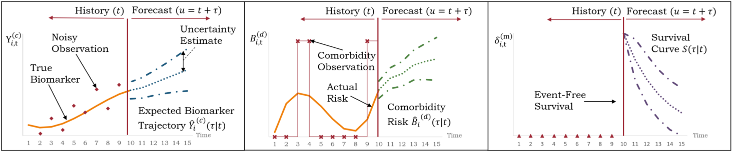
Figure 1: Illustration of Disease-Atlas Predictions over Time

To overcome the limitations of joint models, we introduce Disease-Atlas - a scalable deep learning approach to forecasting disease trajectories over time. Our main contributions are as follows:

Deep Learning for Joint Models

We provide a novel conception of the joint modeling framework using deep learning, capturing the relationships between trajectories through shared representations learned directly from data, and improving scalability as a whole. The network outputs parameters of predictive distributions for longitudinal and time-to-event data that take a similar form to the sub-models used in joint modeling. To the best of our knowledge, this paper is the first to investigate the use of deep learning in joint models for longitudinal and survival trajectories.

Robustness to Irregular Sampling via Multitask Learning

Observations in longitudinal studies are very rarely aligned at every time step, as measurements can be collected at different sampling frequencies. Hence, training a multioutput neural network would require the imputation of the target labels as a pre-processing step, so as to artificially align the dataset prior to calibration. This could lead to poorer predictions if imputation quality is low and a high degree of missingess is present, as the network is biased to simply learn the imputation mechanism. To mitigate this issue, we formulate joint model calibration as a multitask learning problem, grouping variables - which are measured at the same time and with similar sampling frequencies - together into tasks, and training the network using only actual observations as target labels.

Incorporating Medical History into Forecasts

While deep learning for medicine has gained popularity in recent times, the majority of methods, such as (Alaa and van der Schaar, 2017; Ranganath et al., 2016), only use covariates at a single time point in making predictions. However, a patient’s medical history could also be informative of her future clinical outcomes, and predictions could be improved by incorporating past information. We integrate historical information into our network using a Recurrent Neural Network (RNN) in the base layer, which contains a memory state that updates over time as new observations come in.

2 Related Work

While the utility of joint models has been demonstrated by its popularity in longitudinal studies, numerous modeling choices exist, each containing its own advantages and limitations (see (Hickey et al., 2016) for a full overview). (Rizopoulos et al., 2014), for example, highlight the sensitivity of predictions to the association structures used, adopting a Bayesian model averaging approach instead to aggregate the outputs of different models over time. In this respect, the flexibility of deep learning has the potential to enhance dynamic predictions with joint models, by directly learning variable relationships from the data itself, and completely removing the need for explicit model specification. In addition, (Hickey et al., 2016; Barrett et al., 2015; Waldmann et al., 2017; Futoma et al., 2016) note performance limitations when applying standard joint models to high-dimensional datasets. These are typically estimated using Expectation Maximization (EM) or Markov Chain Monte Carlo (MCMC) sampling methods, which rapidly grow in complexity with the number of covariates and random effects. As such, most studies and software packages often focus on modeling a single or a small number of longitudinal measurements, along with a time-to-event of interest. However, the increase in data availability through electronic health records opens up the possibility of using information from multiple trajectories to improve predictions. Recent works have attempted to address this limitation by exploiting special properties of the longitudinal sub-models, such as the multivariate skew-normal structure in (Barrett and Su, 2017), and the combination of variational approximation and dynamic EM-style updates over time in (Futoma et al., 2016). In light of this, the use of deep learning holds much promise in enhancing the performance of joint models, given its inherent ability to scale with large datasets without the need for specific modeling assumptions.

Deep learning has seen increasing use in medical applications, with successes in traditional survival analysis (Ranganath et al., 2016; Luck et al., 2017) survival analysis with competing risks (Lee et al., 2018; Alaa and van der Schaar, 2017) and treatment recommendations (Katzman et al., 2016). In general, these methods focus purely on forecasting survival, do not consider dynamic prediction over time and only use covariates at a single time point in making predictions. Deep Kalman Filters (Krishnan et al., 2017) use a network which does dynamically update its latent states over time but assumes that all outputs follow the same distribution. This prevents it from being applied to heterogeneous datasets, which limits its usage for joint modeling.

RNNs with multitask learning have also been used extensively in making predictions inside the hospital, using frequently sampled measurements as inputs for event detection or automated diagnosis ((Harutyunyan et al., 2017; Razavian et al., 2016; Li et al., 2015; Lipton et al., 2016)). In addition to the characteristics of in-hospital data (i.e. sampled at hourly intervals with a high rate of missing data), these works bear several fundamental differences to the Disease-Atlas. Firstly, in-hospital predictions focus on separate dynamic classification tasks which produce single class labels at each time step, such as the most likely event or diagnosis at the next time step. In contrast, the Disease-Atlas allows for the simultaneous prediction of multiple variables of interest at each time step, which can be either discrete (classification) or continuous (regression). As predictions are conditioned on the same latent structure, we can analyze variables in a consistent fashion and use trajectory forecasts to understand changes in survival probabilities. For example, poorer survival odds could be a result of increased risk of multiple infections. Secondly, the RNNs in existing works typically produce single point forecasts, which do not account for the uncertainty of the model. We address this limitation using the Monte-Carlo Dropout procedure of (Gal and Ghahramani, 2016) (see Section 4.3), producing predictions with uncertainty estimates at each time step.

3 Problem Definition

For a given longitudinal study, let there be $N$ patients with observations made at time $t$, for $0\leq t\leq T_{cens}$ where $T_{cens}$ denotes an administrative censoring time . For the $i^{th}$ patient at time $t$, observations are made for a $K$-dimensional vector of longitudinal variables $\mathbf{V_{i,t}}=[Y_{i,t}^{(1)},\dots,Y_{i,t}^{(C)},B_{i,t}^{(1)},\dots,B_{i,t}^{(D)}]$, where $Y_{i,t}^{(c)}$ and $B_{i,t}^{(d)}$ are continuous and discrete longitudinal measurements respectively, a $L$-dimensional vector of external covariates $\mathbf{X_{i,t}}=[X_{i,t}^{(1)},\dots X_{i,t}^{(L)}]$, and a $M$-dimensional vector of event occurrences $\mathbf{\delta_{i,t}}=[\delta_{i,t}^{(1)},\dots,\delta_{i,t}^{(M)}]$ , where $\delta_{i,t}^{(m)}\in\{0,1\}$ is an indicator variable denoting the presence or absence of the $m^{th}$ event. $T_{i,t}^{(m)}$ is defined to be the first time the event is observed after $t$, which allows us to model both repeated events and events that lead to censoring (e.g. death). The final observation for patient i occurs at $T_{i,\max}=\min(T_{cens},T_{i,0}^{(a_{1})},\dots,T_{i,0}^{(a_{\max})})$, where $\{a_{i},\dots,a_{\max}\}$ is the set of indices for events that censor observations. Furthermore, we introduce a filtration $\mathcal{F}_{i,t}$ to capture the full history of longitudinal variables, external covariates and event occurrences of patient $i$ until time $t$.

3.1 Joint Modeling

From (Hickey et al., 2016), numerous sub-models for longitudinal measurements exist, each with their own pros and cons. General forms for continuous and binary longitudinal measurements are typically expressed as:

$$\begin{split}&Y_{i,u}^{(c)}|\mathcal{F}_{i,t}\sim\text{N}\left(m^{(c)}\left(u,\mathcal{F}_{i,t};\mathbf{b}_{i},\tilde{\mathbf{W}}\right),\sigma_{u}^{(c)~{}2}\right)\end{split}$$ (1)

$$\begin{split}&B_{i,u}^{(d)}|\mathcal{F}_{i,t}\sim\text{Bernoulli}\left(\Phi^{(d)}\left(u,\mathcal{F}_{i,t};\mathbf{b}_{i},\tilde{\mathbf{W}}\right)\right)\end{split}$$ (2)

Where $m^{(c)}(.)$ is a function for the predictive mean of the $c$-th longitudinal variable, and $\sigma_{t}^{(c)~{}2}$ its variance. $\Phi^{(d)}(.)$ is a function for the probability of the binary observation, such as the commonly used logit or probit functions, and $\tilde{\mathbf{W}}$ is the vector of static coefficients used by the sub-models.

In both models, $\mathbf{b}_{i}$ is a vector of association parameters used across trajectories, and define the association structure of the joint model. While the majority of models use subject-specific random effects, this can also refer to time-dependent latent variables as seen in (Ibrahim et al., 2004) or shared spline coefficients in (Barrett and Su, 2017).

Event times can be expressed using the general form below:

$$\begin{split}&T_{i,t}^{(m)}|\mathcal{F}_{i,t}\sim\mathcal{S}\left(\Lambda^{(m)}\left(t,\mathcal{F}_{i,t};\mathbf{b}_{i},\tilde{\mathbf{W}}\right)\right)\end{split}$$ (3)

Where $\mathcal{S}$ is an appropriate survival distribution (e.g. Exponential, Weibull, etc), and $\Lambda^{(m)}(.)$ is a generic cumulative hazard function. In most joint model applications, this typically takes the form of the Cox proportional hazards model.

The standard linear mixed effects models can be expressed as:

$$\begin{split}Y_{i,t}^{(c)}&=\mathbf{X}_{i,t}^{\top}~{}\mathbf{\theta}_{fix}^{(c)}+\mathbf{R}_{i,t}^{\top}~{}\mathbf{\theta}^{(c)}_{rand}+\epsilon^{(c)}_{i,t}\\ &=m^{(c)}(t)+\epsilon^{(c)}_{t}\end{split}$$ (4)

$$h_{i,t}^{(m)}=h_{0}(t)\exp\left(\mathbf{B}_{i}^{\top}\mathbf{\gamma}^{(m)}+\beta^{(m)}m^{(c)}(t)\right)$$ (5)

Where $\mathbf{X}_{i,t}$ and $\mathbf{R}_{i,t}$ are time-dependent design vectors for fixed effects $\mathbf{\theta}_{fix}^{(c)}$ and random effects $\mathbf{\theta}^{(c)}_{rand}$, $\epsilon_{i,t}^{(c)}\sim N\left(0,\sigma_{t}^{(c)~{}2}\right)$ is a random noise term, and $h_{i,t}^{(m)}$ is the hazard rate of the survival process, with patient fixed covariates $\mathbf{B}_{i}$, and static coefficients $\gamma^{(m)}$ and $\beta^{(m)}$.

In this model, we define the association parameters of the joint model to be those common to both longitudinal and survival processes, i.e $\mathbf{b}_{i}=[\mathbf{\theta}_{fix}^{(c)}$, $\mathbf{\theta}^{(c)}_{rand}]$, and static coefficients which are unique to the separate processes, i.e. $\mathbf{\tilde{W}}=[\gamma^{(m)},\beta^{(m)}]$.

3.2 Dynamic Prediction

Dynamic prediction in joint models can be defined as the estimation of both the expected values of longitudinal variables and survival probabilities over a specific time window $\tau$ in the future:

$$\hat{V}_{i}^{(k)}(\tau|t)=\mathbb{E}\left[V_{i,t+\tau}^{(k)}|\mathcal{F}_{i,t};\mathbf{b}_{i},\tilde{\mathbf{W}}\right]$$ (6)

$$\begin{split}&S_{i}^{(m)}(\tau|t)=P\left(T_{i,0}^{(m)}\geq t+\tau|T_{i,0}^{(m)}\geq t,\mathcal{F}_{i,t};\mathbf{b}_{i},\tilde{\mathbf{W}}\right)\end{split}$$ (7)

Where $V_{i,t}^{(k)}$ is the $k^{th}$ longitudinal variable at time t that can be either continuous or binary. A conceptual illustration of dynamic prediction can be found in Figure 1. For continuous longitudinal variables, such as biomarker predictions, the goal is to forecast its expected value given all the information until the current time step (i.e. $\mathcal{F}_{i,t}$). In the case of binary observations, such as the presence of a comorbidity, the expectation in Equation 6 is the probability (or risk) of developing a comorbidity at time $t+\tau$. The survival curves shown give us the probability of not experiencing an event over various horizons $\tau$ given $\mathcal{F}_{i,t}$. While the uncertainty estimates are model dependent, these are usually expressed via confidence intervals in frequentist methods, or using the posterior distributions for $\mathbf{b}_{i,t}$ and $\tilde{\mathbf{W}}$ in Bayesian models.

4 Network Design

4.1 Architecture

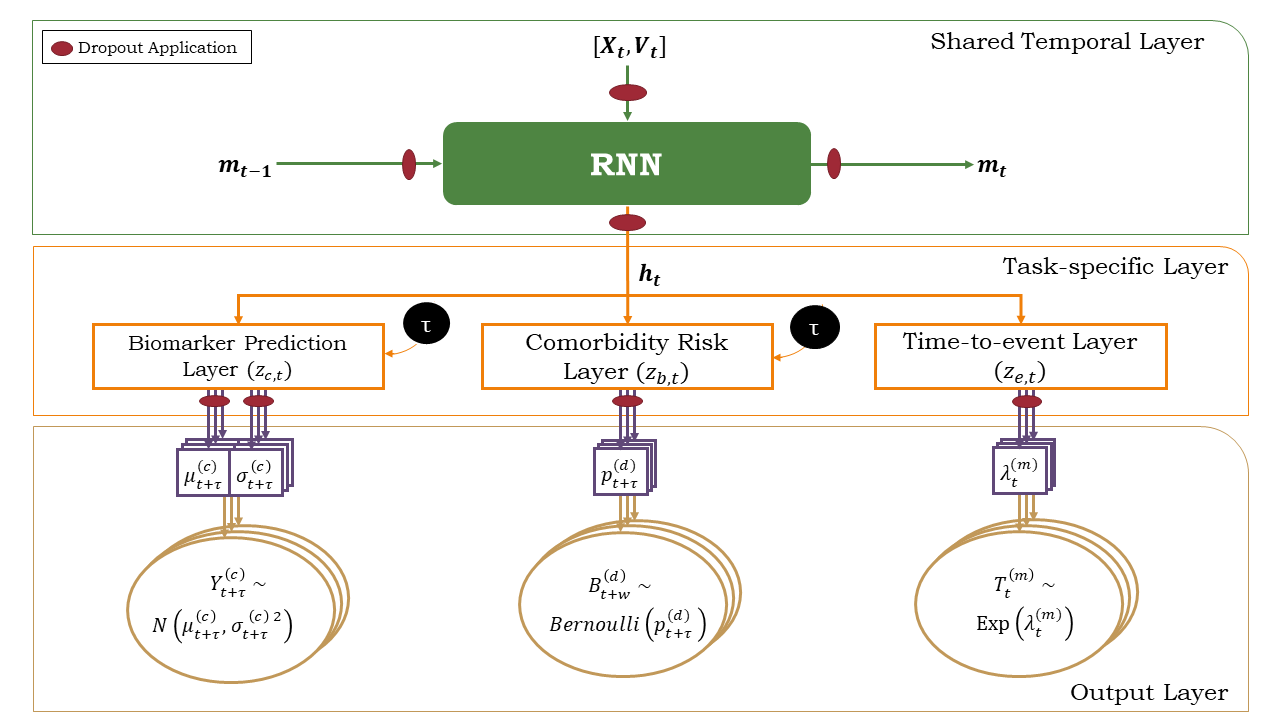
Figure 2: Disease-Atlas Network Architecture

Disease-Atlas captures the associations within the joint modeling framework, by learning shared representations between trajectories at different stages of the network, while retaining the same sub-model distributions captured by joint models. The network, as shown in Figure 2, is conceptually divided into 3 sections: 1) A shared temporal layer to learn the temporal and cross correlations between variables, 2) task-specific layers to learn shared representations between related trajectories, and 3) an output layer which computes parameters for predictive sub-model distributions for use in likelihood loss computations during training and generating predictive distributions at run-time.

The equations for each layer are listed in detail below. For notational convenience, we drop the subscript $i$ for variables in this section, noting that the network is only applied to trajectories from one patient at time.

Shared Temporal Layer

We start with an RNN at the base of the network, which incorporates historical information (i.e. $\mathcal{F}_{t}$) into forecasts by updating its memory state over time. For the tests in Section 5, the usage of both the Simple Recurrent Network (SRN) and LSTM in this layer was compared.

$$[\mathbf{h_{t}},\mathbf{m_{t}}]=\text{RNN}([\mathbf{X_{t}},\mathbf{V_{t}}],\mathbf{m_{t-1}})$$ (8)

Where $\mathbf{h_{t}}$ is the output of the RNN and $\mathbf{m_{t}}$ its memory state. To generate uncertainty estimates for forecasts and retain consistency with joint models, we adopt the MC dropout approach described in (Gal and Ghahramani, 2016). Dropout masks are applied to the inputs, memory states and outputs of the RNN, and are also fixed across time steps. For memory updates, the RNN uses the Exponential Linear Unit (ELU) activation function.

Task-specific Layers

For the task-specific layers, variables are grouped according to the sub-model types in Section 3.1, with layer $\mathbf{z_{c,t}}$ for continuous-valued longitudinal variables, $\mathbf{z_{b,t}}$ for binary longitudinal variables and $\mathbf{z_{e,t}}$ for events. Dropout masks are also applied to the outputs of each layer here. At the inputs to the continuous and binary task layers, a prediction horizon $\tau$ is also concatenated with the outputs from the RNN. This allows the parameters of the predictive distributions at $t+\tau$ to be computed in the final layer, i.e. $\mathbf{\tilde{h}_{t}}=\left[\mathbf{h}_{t},\tau\right]$.

$$\mathbf{z_{c,t}}=\text{ELU}(\mathbf{W_{c}}\mathbf{\tilde{h}_{t}}+\mathbf{a_{c}})$$ (9a)

$$\mathbf{z_{b,t}}=\text{ELU}(\mathbf{W_{b}}\mathbf{\tilde{h}_{t}}+\mathbf{a_{b}})$$ (9b)

$$\mathbf{z_{e,t}}=\text{ELU}(\mathbf{W_{e}}\mathbf{h_{t}}+\mathbf{a_{e}})$$ (9c)

Output Layer

The final layer computes the parameter vectors of the predictive distribution, which are used to compute log likelihoods during training and dynamic predictions at run-time.

$$\mathbf{\mu_{t+\tau}} =\mathbf{W_{\mu}}\mathbf{z_{c,t}}+\mathbf{a_{\mu}}$$ (10a)

$$\mathbf{\sigma_{t+\tau}} =\text{Softplus}(\mathbf{W_{\sigma}}\mathbf{z_{c,t}}+\mathbf{a_{\sigma}}))$$ (10b)

$$\mathbf{p_{t+\tau}} =\text{Sigmoid}(\mathbf{W_{p}}\mathbf{z_{b,t}}+\mathbf{a_{p}}))$$ (10c)

$$\lambda_{t} =\text{Softplus}(\mathbf{W_{\lambda}}\mathbf{z_{e,t}}+\mathbf{a_{\lambda}}))$$ (10d)

Softplus activation functions are applied to $\mathbf{\sigma_{t+\tau}}$ and $\mathbf{p_{t+\tau}}$ to ensure that we obtain valid (i.e. $\geq 0$) standard deviations and binary probabilities. For simplicity, the exponential distribution is selected to model survival times, and predictive distributions can be expressed in a similar manner to that of Section 3.1:

$$Y_{t+\tau}^{(c)} \sim N\left(\mu_{t+\tau}^{(c)},\sigma_{t+\tau}^{(c)2}\right)$$ (11a)

$$B_{t+\tau}^{(d)} \sim\text{Bernoulli}\left(p_{t+\tau}^{(d)}\right)$$ (11b)

$$T_{t}^{(m)} \sim\text{Exponential}\left(\lambda_{t}^{(m)}\right)$$ (11c)

4.2 Multitask Learning

From the above, the negative log-likelihood of the data given the network is:

$$\mathcal{L}(\mathbf{W})=\sum_{i,t,w,k_{c},k_{b},m}-\biggl{[} \log f_{c}\left(Y_{i,t+\tau}^{(c)}|\mu_{t+\tau}^{(c)},\sigma_{t+\tau}^{(c)2},\mathbf{W}\right)+\log f_{b}\left(B_{i,t+\tau}^{(d)}|p_{t+\tau}^{(d)},\mathbf{W}\right)$$

$$+\log f_{T}\left(T_{i,t}^{(m)}|\lambda_{t}^{(m)},\mathbf{W}\right)\biggr{]}$$ (12)

Where $f_{c}(.),f_{b}(.)$ are likelihood functions based on Equations 11 and $\mathbf{W}$ collectively represents the weights and biases of the entire network. For survival times, $f_{T}(.)$ is given as:

$$f_{T}\left(T_{t}^{(m)}|\lambda_{t}^{(m)},\mathbf{W}\right)=\left(\lambda_{t}^{(m)}\right)^{\delta_{i,T}}\exp\left(-\lambda_{t}^{(m)}T_{t}^{(m)}\right)$$ (13)

Which corresponds to event-free survival until time T before encountering the event (Dunteman and Ho, 2006). While the negative log-likelihood can be directly optimized across tasks, the use of multitask learning can yield the following benefits:

Better Survival Representations

As shown in (Li et al., 2015), multitask learning problems which have one main task of interest can weight the individual loss contributions of each subtask to favor representations for the main problem. For our current architecture, where we group similar tasks into task-specific layers, our loss function corresponds to:

$$L(\mathbf{W})= -\underbrace{\alpha_{c}\sum^{i,t,w,c}\log f_{c}\left(Y_{t+\tau}^{(c)}|\mathbf{W}\right)}_{\text{Continuous Longitudinal Loss }l_{c}}-\underbrace{\alpha_{b}\sum^{i,t,w,d}\log f_{b}\left(B_{t+\tau}^{(d)}|\mathbf{W}\right)}_{\text{Binary Longitudinal Loss }l_{b}}$$

$$-\underbrace{\alpha_{T}\sum^{i,t,m}\log f_{T}\left(T_{t}^{(m)}|\mathbf{W}\right)}_{\text{Time-to-event Loss }l_{T}}$$ (14)

Given that survival predictions are the primary focus of many longitudinal studies, we set $\alpha_{c}=\alpha_{b}=1$ and include $\alpha_{T}$ as an additional hyperparameter to be optimized. To train the network, patient trajectories are subdivided into Q sets of $\Omega_{q}(i,\rho,\tau)=\left\{\mathbf{X_{i,{0:\rho}}},\mathbf{Y_{i,\rho+\tau}},\mathbf{T_{max,i}},\mathbf{\delta_{i}}\right\}$, where $\rho$ is the length of the covariate history to use in training trajectories up to a maximum of $\rho_{\max}$. Our procedure follows that of (Collobert and Weston, 2008), as detailed in Algorithm 1.

Handling Irregularly Sampled Data

We address issues with irregular sampling by grouping variables that are measured together into the same task, and training the network with multitask learning. For instance, height, weight and BMI measurements are usually taken at the same time during follow-up, and can be grouped together in the same task. Given the completeness of the datasets we consider, we assume that task groupings match those defined by the task-specific layer of the network, and multitask learning is performed using Equation 4.2 and Algorithm 1.

We note, however, that in the extreme case where none of the trajectories are aligned, we can define each variable as a separate task with its own loss function $l_{*}$. Algorithm 1 then samples loss functions for one variable at a time, and the network is trained using only actual observations as target labels. This could reduce errors in cases where multiple sample rates exist and simple imputation is used, which might result in the multioutput networks replicating the imputation process instead of making true predictions.

Algorithm 1 Training Disease-Atlas

  Input: Data $\Omega=\{\Omega_{1},\dots,\Omega_{Q}\}$, max iterations $\mathcal{J}$

  Output: Calibrated network weights $\mathbf{W}$

  for  count$=1$ to $\mathcal{J}$ do

     Get minibatch $\mathcal{M}\sim$ $\gamma$ random samples from $\Omega$

     Sample task loss function $l\sim\{l_{c},l_{b},l_{T}\}$

     Update $\mathbf{W}\leftarrow\texttt{Adam}(l,\mathcal{M})$, using feed-forward passes with dropout applied

  end for

4.3 Forecasting Disease Trajectories

Dynamic prediction involves 2 key elements - 1) calculating the expected longitudinal values and survival curves as described in Section 3.2, and 2) computing uncertainty estimates. To obtain these measures, we apply the Monte-Carlo dropout approach of (Gal and Ghahramani, 2016) by approximating the posterior over network weights as:

$$p(V^{(k)}_{t+\tau}|\mathcal{F}_{t})\approx\frac{1}{J}\sum_{j=1}^{J}p(V^{(k)}_{t+\tau}|\mathcal{F}_{t},\hat{\mathbf{W}}_{j})$$ (15)

Where we draw $J$ samples $\hat{\mathbf{W}}_{j}$ using feed-forward passes through the network with the same dropout mask applied across time-steps. The samples obtained can then be used to compute expectations and uncertainty intervals for forecasts.

5 Tests on Medical Data

5.1 Overview of Datasets

The UK Cystic Fibrosis (CF) registry contains data obtained for a cohort of 10980 CF patients during annual follow ups between 2008-2015, with a total of 87 variables associated with each patient across all years. In our investigations below, we consider a joint model for 2 continuous lung function scores (FEV1 and Predicted FEV1), 20 comorbidity and infection risks (treated as binary longitudinal observations) as well as death as the event of interest, simultaneously forecasting them all at each time step. We refer the reader to Appendix A for a full breakdown of the dataset.

5.2 Benchmarks and Training Procedure

We compared the Disease-Atlas (DA) against simpler neural networks i.e. LSTM and Multi-layer Perceptrons (MLP), and traditional dynamic prediction methods, i.e. landmarking (L) (van Houwelingen and Putter, 2011) and joint models (JM). The data was partitioned into 3 sets: a training set with 60% of the patients, a validation set with 20% and a testing set with the final 20%. Hyper-parameter optimization was performed using 20 iterations of random search on the validation data, and the test set was reserved for out-of-sample testing. Full details on the training procedure can be found in Appendix A. Models were compared using several metrics: Mean-Squared Error (MSE) for predictions of continuous longitudinal variables, and the area under the Receiver Operating Characteristic (AUROC) and Precision-Recall Curve (AUPRC) for binary variables and the event of interest, i.e. death. Predictions were made via the MC dropout procedure described in Section 4.3, with expectations computed using 300 samples per time step.

Disease-Atlas

Through subsequent tests, we demonstrate the performance contributions of the different innovations of Disease-Atlas, namely the usage of multitask learning in the presence of irregular sampling (Section 5.3), and the inclusion of the RNN in the base layer for temporal information (Section 5.4). For the temporal layer, we evaluate the use of both a LSTM (DA-LSTM) or a single ELU layer (DA-NN).

Standard Neural Networks

Both the LSTM and MLP were taken to be benchmarks, structured to produce the same output distribution parameters as the Disease-Atlas, and optimized according to the multioutput loss function in Equation 4.2. This makes the benchmarks equivalent to the DA-LSTM and DA-NN structures without task-specific layers and input $\tau$, and restricts them to making one-step-ahead longitudinal predictions only.

Landmarking

For consistency with other studies of Cystic Fibrosis (MacKenzie et al., 2014), we use age as the time variable, and fit separate Cox regression models for patients in different age groups ($<25$, $25-50$, $50-75$ and $>75$ years old). As data is left-truncated with respect to age, we use the entry-exit implementation of the Cox proportional hazards model implemented in (Therneau, 2015). To avoid issues with collinearity, we start with a preliminary feature selection step first - performing multi-step Cox regression on the validation dataset, and only retaining features with coefficient p-values $<0.1$.

Joint Models

With the computational limitations of standard joint models, direct application to our dataset - containing over 6,500 patients in the training set with 87 annual covariate measurements - proved to be infeasible. As such, we used the two-step estimation procedure of (Wu, 2009), fitting the individual linear mixed effects (LME) longitudinal sub-models first, and using the mean estimates in the Cox regression model. For continuous variables, the linear mixed effects models used random intercepts and slopes, this is in line with the FEV1 models in (van Horck et al., 2017), (Van Diemen et al., 2011) and (Stern et al., 2007). For binary variables, we use the logit regression version of the LME model, as implemented in the lme4 R package (Bates et al., 2015).

5.3 Evaluating Multitask Learning with Irregularly Sampled Data

To evaluate the effectiveness of multitask learning, we simulate irregular sampling by randomly removing all data points across each task (defined in Section 4.2) with a probability $\gamma$ at every time step. For multivariate prediction, continuous-valued inputs were imputed using the mean value of the training set, while binary variables and indicators of death were set to 0. The networks were trained according to Section 4.2, and then evaluated on the complete test set based on 1) MSE for continuous variables, and 2) AUROC for binary/event predictions.

Figure 3 shows the outperformance of multitask learning, which has a lower MSE for FEV1 and higher AUROCs for comorbidity and mortality predictions as $\gamma$ increases. The improvements are most pronounced for MSE, as FEV1 has values at every time step, as opposed to binary observations and occurrences of death which are relatively more infrequent in the dataset. This demonstrates the robustness of the model to irregular sampling, and provides a way for joint models to be used on datasets even under such conditions.

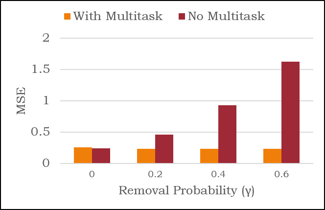
(a) FEV1 MSE

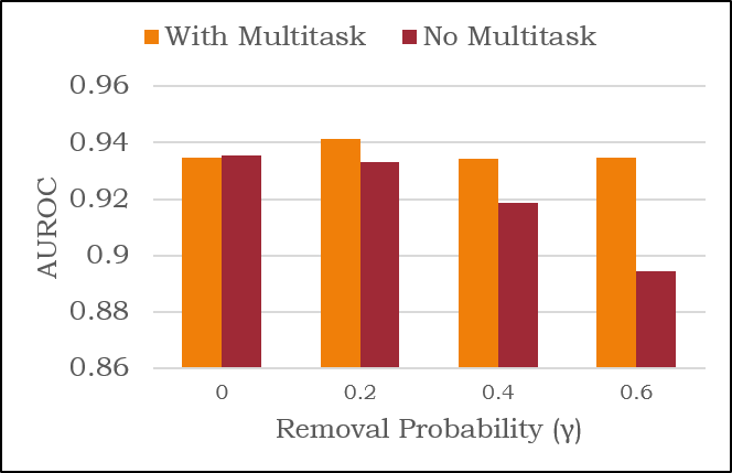
(b) Comorbidity AUROC

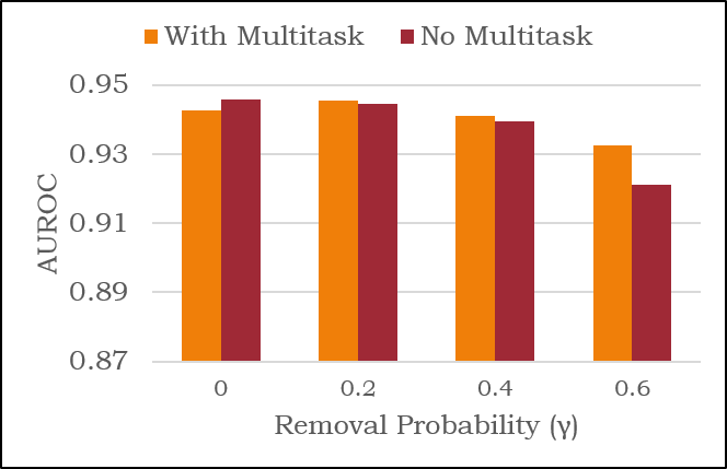
(c) Mortality AUROC

Figure 3: Performance Comparison Between Multitask and Multioutput Networks

5.4 Performance vs Benchmarks

As survival analysis is the usually main task of interest, we perform a comprehensive evaluation across all benchmarks, computing a probability of the event of interest, i.e. death, at a given time step using $1-S_{i}^{(m)}(\tau|t)$ from Equation 7. Performance was compared on the basis of AUROC and AUPRC of mortality predictions at various horizons $\tau$. To account for the stochastic nature of the MC dropout sampling procedure, performance evaluation was repeated 3 times for each neural network, with the averages and standard deviations of the metrics in reported in Table 1.

Table 1: Results of Mortality Predictions for Cystic Fibrosis (Mean $\pm$ S.D. Across 3 Runs)

	$\tau$	DA-LSTM	DA-NN	LSTM	MLP	L	JM
AUROC	1	0.944($\pm$ 0.0004)	0.943($\pm$ 0.0003)	0.943($\pm$ 0.0007)	0.941($\pm$ 0.0003)	0.824	0.870
	2	0.924($\pm$ 0.0008)	0.923($\pm$ 0.0005)	0.923($\pm$ 0.0005)	0.919($\pm$ 0.0003)	0.812	0.870
	3	0.910($\pm$ 0.0003)	0.905($\pm$ 0.0002)	0.908($\pm$ 0.0002)	0.907($\pm$ 0.0002)	0.825	0.851
	4	0.905($\pm$ 0.0003)	0.902($\pm$ 0.0008)	0.904($\pm$ 0.0003)	0.904($\pm$ 0.0006)	0.776	0.828
	5	0.895($\pm$ 0.0003)	0.892($\pm$ 0.0005)	0.894($\pm$ 0.0005)	0.888($\pm$ 0.0007)	0.765	0.806
AUPRC	1	0.278 ($\pm$ 0.0037)	0.238 ($\pm$ 0.0040)	0.230 ($\pm$ 0.0020)	0.219 ($\pm$ 0.0036)	0.161	0.119
	2	0.193 ($\pm$ 0.0014)	0.169 ($\pm$ 0.0033)	0.165 ($\pm$ 0.0017)	0.186 ($\pm$ 0.0036)	0.082	0.092
	3	0.103 ($\pm$ 0.0005)	0.092 ($\pm$ 0.0007)	0.099 ($\pm$ 0.0028)	0.105 ($\pm$ 0.0001)	0.085	0.089
	4	0.109 ($\pm$ 0.0007)	0.101 ($\pm$ 0.0014)	0.095 ($\pm$ 0.0010)	0.102 ($\pm$ 0.0006)	0.062	0.068
	5	0.101 ($\pm$ 0.0007)	0.091 ($\pm$ 0.0008)	0.093 ($\pm$ 0.0017)	0.100 ($\pm$ 0.0017)	0.058	0.059

The first thing to note is the vast improvements of neural networks over traditional dynamic prediction models, with the DA-LSTM showing average AUPRC improvements of $75\%$ and $78\%$ across all time steps when compared to landmarking and standard joint models. Among the neural network benchmarks, the strongest gains for the DA-LSTM can be seen over shorter prediction horizons (1-2 years), improving the DA-NN by $17\%$ and the LSTM by $21\%$ in one-step-ahead AUPRC. This highlights the benefits of both the use of temporal information and the addition of task-specific layers for short-term survival predictions. While the gains in AUROC are indeed smaller, this can be attributed to the large class imbalance present within the dataset, due to the rare occurrence of death in the dataset (seen in 451 of 10275 patients) and the censoring effect it has on a patients trajectory. As shown in (Saito and Rehmsmeier, 2015), ROC metrics can lead to deceptive good performance, as the definition of the false positive rate (false positive / total number of negatives) permits the occurrence of a large number of false positives in imbalanced datasets, and recommend the use of PRC metrics. In addition, we note that the Disease-Atlas architectures also allow for the forecasting of longitudinal variables over arbitrary horizons, which standard neural network architectures are unable to accommodate by default.

Table 2: Results of Longitudinal Predictions for Cystic Fibrosis (Single Run)

MSE AUROC [Mean $\pm$ SD] AUPRC [Mean $\pm$SD] $\tau$ FEV1 Pred. FEV1 Comorbidities Infections Comorbidities Infections DA-LSTM 1 0.182 121.3 0.957 ($\pm$ 0.025) 0.888 ($\pm$ 0.056) 0.680 ($\pm$0.261) 0.416 ($\pm$0.247) 2 0.191 139.4 0.926 ($\pm$0.047) 0.850 ($\pm$ 0.044) 0.648 ($\pm$ 0.244) 0.337 ($\pm$ 0.261) 3 0.275 191.3 0.882 ($\pm$0.048) 0.798 ($\pm$ 0.057) 0.555 ($\pm$ 0.213) 0.337 ($\pm$ 0.261) 4 0.374 254.4 0.817 ($\pm$0.085) 0.723 ($\pm$ 0.068) 0.459 ($\pm$ 0.184) 0.309 ($\pm$ 0.252) 5 0.461 308.1 0.790 ($\pm$0.067) 0.669 ($\pm$ 0.126) 0.388 ($\pm$ 0.169) 0.269 ($\pm$ 0.247) JM 1 0.553 368.6 0.699 ($\pm$ 0.148) 0.673 ($\pm$ 0.069) 0.176 ($\pm$ 0.088) 0.161 ($\pm$ 0.176) 2 0.593 411.1 0.694 ($\pm$ 0.139) 0.651 ( $\pm$ 0.060) 0.180 ( $\pm$ 0.089) 0.157 ( $\pm$ 0.181) 3 0.641 451.8 0.685 ($\pm$ 0.140) 0.631 ( $\pm$ 0.072) 0.185 ( $\pm$ 0.090) 0.160 ( $\pm$ 0.186) 4 0.695 490.1 0.681 ($\pm$ 0.132) 0.607 ( $\pm$ 0.077) 0.187 ( $\pm$ 0.091) 0.159 ( $\pm$ 0.188) 5 0.750 519.7 0.673 ($\pm$ 0.130) 0.580 ( $\pm$ 0.082) 0.188 ( $\pm$ 0.093) 0.155 ( $\pm$ 0.186)

We proceed to evaluate the longitudinal forecasting ability of the Disease-Atlas in Table 2, focusing on comparisons between the DA-LSTM and standard joint models. To provide a concise summary of longitudinal prediction results, we use a single set of 300 MC dropout samples to compute performance metrics. The average AUROC/AUPRC for comorbidities and infections are reported separately, along with standard deviations across each group. Similarly, results for FEV1 and Predicted FEV1 are reported for a single evaluation, and a full breakdown of results for each individual binary longitudinal variable is detailed in Appendix A. We can see that the DA-LSTM improves performance across all longitudinal prediction categories, reducing MSEs by $56\%$ on average across all continuous predictions, and improving AUPRCs in comorbidities and infections on average by $199\%$ and $112\%$ respectively. This vast improvement underscores the ability of deep neural networks to learn complex interactions directly from the data, and demonstrates the benefits of using a deep learning approach to joint modeling.

6 Illustrative Use Case for Disease-Atlas: Personalized Screening

While numerous use cases for the Disease-Atlas exist, one possible example is its use in personalized screening, i.e. prescribing testing regimes and follow-up schedules that are tailored to the unique characteristics of a patient. (Ahuja et al., 2017) derive an optimal policy that balances the costs of screening, along with the risks of delaying the screening process. Their paper, however, has two important limitations: 1) it requires the evolution of the disease to be known, and 2) it requires an analytical expression for the cost of delay, which is often difficult to determine in practice. Disease-Atlas does not suffer from these limitations.

We illustrate how the Disease Atlas can be used for identifying screening profiles for Cystic Fibrosis patients. We use as an exemplar an actual patient from our test set who started to be seen in 2008 and is screened for Diabetes, a very important comorbidity affecting the treatment of patients.

Figure 4 shows how the Disease Atlas can be used to design personalized screening policies. Using the Disease Atlas as applied from 2008-2010, we can record the “smoothed” estimate at each time step, i.e. $\hat{B}_{i}^{(d)}(0|t)$ as per Equation 6 and plotted in orange. To determine a patient’s future risk, we extrapolate in the usual way over various horizons $\tau$, providing both the expected value and an uncertainty interval using the 5th and 95th percentiles of the MC dropout samples. From Figure 6, we see that the patient had a steady 18% increase in risk from 2008 to 2010, and will expect a further increase of 13% over the next 5 years. Informed by the Disease Atlas, the clinician may decide to prescribe additional tests for Diabetes, or increase the frequency of follow-up in the short-term to better monitor risks.

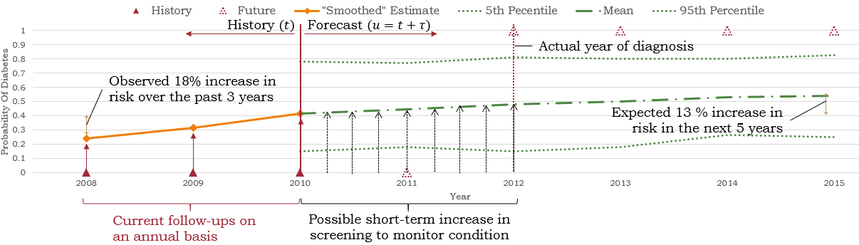
Figure 4: Using Disease-Atlas for Personalized Screening

Appendix for Disease-Atlas

Appendix A Tests on Cystic Fibrosis Dataset

A.1 Details on Dataset

The UK Cystic Fibrosis (CF) registry contains data obtained for a cohort of 10980 CF patients during annual follow ups between 2008-2015, with a total of 87 variables that were associated with each patient across all years. This includes demographic information (e.g. age, height, weight, BMI), genetic information, treatments received, metrics for lung function (FEV1 and Predicted FEV1), comorbidities observed, and any bacterial infections developed. In our investigations, we consider a joint model for the 2 continuous lung function scores (FEV1 and Predicted FEV1), 20 binary longitudinal variables of comorbidity and infection, along with death as the event of interest.

A full description of the jointly-modeled longitudinal and time-to-event datasets can be found in Table 3.

Table 3: Description of Longitudinal and Time-to-event Data for CF

		Type	% Patients	Mean	S.D.	Min	Max
Event	Death	Binary (Event)	4.70%	0.008	0.087	0.000	1.000
Biomarkers	FEV1	Continuous	100.00%	2.176	0.914	0.090	6.250
	Predicted FEV1	Continuous	100.00%	72.109	22.404	8.950	197
Comorbidities	Liver Disease	Binary	20.80%	0.128	0.334	0.000	1.000
	Asthma	Binary	22.96%	0.146	0.353	0.000	1.000
	Arthropathy	Binary	9.50%	0.050	0.218	0.000	1.000
	Bone fracture	Binary	1.94%	0.007	0.081	0.000	1.000
	Raised Liver Enzymes	Binary	23.91%	0.114	0.318	0.000	1.000
	Osteopenia	Binary	20.37%	0.114	0.318	0.000	1.000
	Osteoporosis	Binary	9.58%	0.051	0.219	0.000	1.000
	Hypertension	Binary	3.30%	0.020	0.139	0.000	1.000
	Diabetes	Binary	24.56%	0.167	0.373	0.000	1.000
Bacterial	Burkholderia Cepacia	Binary	5.59%	0.034	0.181	0.000	1.000
Infections	Pseudomonas Aeruginosa	Binary	65.18%	0.407	0.491	0.000	1.000
	Haemophilus Influenza	Binary	30.55%	0.091	0.288	0.000	1.000
	Aspergillus	Binary	29.29%	0.110	0.313	0.000	1.000
	NTM	Binary	6.38%	0.019	0.136	0.000	1.000
	Ecoli	Binary	5.32%	0.012	0.111	0.000	1.000
	Klebsiella Pneumoniae	Binary	4.93%	0.010	0.101	0.000	1.000
	Gram-Negative	Binary	3.78%	0.008	0.089	0.000	1.000
	Xanthomonas	Binary	13.18%	0.043	0.202	0.000	1.000
	Staphylococcus Aureus	Binary	52.59%	0.244	0.429	0.000	1.000
	ALCA	Binary	5.06%	0.020	0.138	0.000	1.000

A.2 Hyperparameter Optimization

Hyperparameter optimization was conducted using 20 iterations of random search, with the search space documented in Table 4. Please note that the RNN state size was defined relative to the number of input features ($L$). The task specific layers were also size in relation to the RNN state size, and defined to be (state size + task output size) /2. This was done to ensure that we had a principled way of sizing the task-specific layer relative to state size and outputs, without having to add on too many additional hyper-parameters (i.e. one per task-specific layer). In addition, $\alpha_{T}$ was defined in relation to the number of longitudinal variables ($K$). All neural networks were trained to convergence, as determined by the survival log-likelihoods evaluated on the validation data, or up to a maximum of 50 epochs.

The final parameters obtained for each network can be found in Table 5.

Table 4: Hyper-parameter Selection Range for Random Search

	Hyper-parameter Selection Range
Max Number of Epochs	50
RNN State Size	1L, 2L, 3L, 4L, 5L
$\alpha_{T}$	K, 2K, 3K, 4K, 5K
Max Gradient Norm	0.5, 1.0, 1.5, 2.0
Learning Rate	1e-3, 5e-3, 1e-4
Minibatch Size	64, 128, 256
Dropout Rate	0.2, 0.3, 0.4, 0.5

Table 5: Hyper-parameters Selected for CF Tests

State Size Minibatch Size Learning Rate Max Gradient Norm Dropout Rate $\alpha_{T}$ DA-LSTM 1L 256 1.00E-04 0.5 0.3 3K DA-NN 5L 256 1.00E-04 2.0 0.3 4K Standard LSTM 1L 32 1.00E-03 1.5 0.4 4K Standard NN 1.5L 64 1.00E-03 1 0.45 1K

A.3 Additional Results

To supplement the results in the test section of the main report, a detailed breakdown of the prediction results for binary longitudinal variables can be found in Table 6 and 7 for DA-LSTM and JM respectively. For the DA-LSTM, due to the randomness present in the MC dropout procedure, the performance evaluation was repeated 3 times with the means and standard deviations reported in the tables. The results also demonstrate the outperformance of the deep neural network over standard benchmarks in both AUROC and AUPRC terms.

Table 6: AUROC for Comorbidity and Infection Predictions for CF Dataset (Mean $\pm$ S.D. Across 3 Runs)

DA-LSTM 1 2 3 4 5 Comorbidities Liver Disease 0.975 ($\pm$ 0.0001) 0.948 ($\pm$ 0.0001) 0.897 ($\pm$ 0.0003) 0.826 ($\pm$ 0.0005) 0.767 ($\pm$ 0.0001) Asthma 0.979 ($\pm$ 0.0001) 0.946 ($\pm$ 0.0002) 0.906 ($\pm$ 0.0005) 0.843 ($\pm$ 0.0004) 0.784 ($\pm$ 0.0003) Arthropathy 0.975 ($\pm$ 0.0004) 0.950 ($\pm$ 0.0002) 0.911 ($\pm$ 0.0004) 0.888 ($\pm$ 0.0007) 0.833 ($\pm$ 0.0004) Bone fracture 0.891 ($\pm$ 0.0024) 0.791 ($\pm$ 0.0015) 0.789 ($\pm$ 0.0014) 0.610 ($\pm$ 0.0029) 0.721 ($\pm$ 0.0013) Raised Liver Enzymes 0.937 ($\pm$ 0.0006) 0.909 ($\pm$ 0.0002) 0.798 ($\pm$ 0.0004) 0.741 ($\pm$ 0.0006) 0.685 ($\pm$ 0.0002) Osteopenia 0.961 ($\pm$ 0.0005) 0.942 ($\pm$ 0.0003) 0.897 ($\pm$ 0.0006) 0.873 ($\pm$ 0.0005) 0.850 ($\pm$ 0.0004) Osteoporosis 0.956 ($\pm$ 0.0006) 0.943 ($\pm$ 0.0008) 0.912 ($\pm$ 0.0006) 0.877 ($\pm$ 0.0008) 0.854 ($\pm$ 0.0003) Hypertension 0.977 ($\pm$ 0.0004) 0.955 ($\pm$ 0.0006) 0.936 ($\pm$ 0.0009) 0.879 ($\pm$ 0.0006) 0.869 ($\pm$ 0.0009) Diabetes 0.963 ($\pm$ 0.0002) 0.942 ($\pm$ 0.0002) 0.918 ($\pm$ 0.0001) 0.873 ($\pm$ 0.0003) 0.844 ($\pm$ 0.0004) Infections Burkholderia Cepacia 0.960 ($\pm$ 0.0011) 0.929 ($\pm$ 0.0009) 0.922 ($\pm$ 0.0008) 0.876 ($\pm$ 0.0004) 0.846 ($\pm$ 0.0011) Pseudomonas Aeruginosa 0.898 ($\pm$ 0.0004) 0.878 ($\pm$ 0.0002) 0.850 ($\pm$ 0.0002) 0.818 ($\pm$ 0.0003) 0.796 ($\pm$ 0.0005) Haemophilus Influenza 0.848 ($\pm$ 0.0007) 0.835 ($\pm$ 0.0002) 0.798 ($\pm$ 0.0002) 0.737 ($\pm$ 0.0007) 0.738 ($\pm$ 0.0012) Aspergillus 0.873 ($\pm$ 0.0007) 0.798 ($\pm$ 0.0004) 0.789 ($\pm$ 0.0007) 0.673 ($\pm$ 0.0010) 0.665 ($\pm$ 0.0006) NTM 0.897 ($\pm$ 0.0008) 0.802 ($\pm$ 0.0013) 0.824 ($\pm$ 0.0014) 0.675 ($\pm$ 0.0008) 0.633 ($\pm$ 0.0002) Ecoli 0.929 ($\pm$ 0.0018) 0.894 ($\pm$ 0.0013) 0.733 ($\pm$ 0.0044) 0.677 ($\pm$ 0.0043) 0.340 ($\pm$ 0.0066) Klebsiella Pneumoniae 0.950 ($\pm$ 0.0012) 0.904 ($\pm$ 0.0007) 0.815 ($\pm$ 0.0044) 0.630 ($\pm$ 0.0005) 0.725 ($\pm$ 0.0046) Gram-Negative 0.745 ($\pm$ 0.0052) 0.793 ($\pm$ 0.0045) 0.690 ($\pm$ 0.0007) 0.698 ($\pm$ 0.0020) 0.587 ($\pm$ 0.0027) Xanthomonas 0.894 ($\pm$ 0.0009) 0.831 ($\pm$ 0.0005) 0.770 ($\pm$ 0.0013) 0.716 ($\pm$ 0.0007) 0.654 ($\pm$ 0.0006) Staphylococcus Aureus 0.908 ($\pm$ 0.0002) 0.856 ($\pm$ 0.0004) 0.784 ($\pm$ 0.0005) 0.699 ($\pm$ 0.0003) 0.649 ($\pm$ 0.0005) ALCA 0.863 ($\pm$ 0.0008) 0.831 ($\pm$ 0.0010) 0.800 ($\pm$ 0.0008) 0.758 ($\pm$ 0.0010) 0.725 ($\pm$ 0.0015) JM 1 2 3 4 5 Comorbidities Liver Disease 0.634 0.622 0.619 0.607 0.602 Asthma 0.701 0.671 0.649 0.622 0.597 Arthropathy 0.761 0.755 0.755 0.757 0.749 Bone Fracture 0.344 0.379 0.378 0.413 0.411 Raised Liver Enzymes 0.622 0.608 0.589 0.584 0.594 Osteopenia 0.774 0.767 0.761 0.758 0.746 Osteoporosis 0.801 0.794 0.781 0.772 0.76 Hypertension 0.894 0.891 0.893 0.893 0.889 Diabetes 0.76 0.754 0.739 0.723 0.709 Infections Burkholderia Cepacia 0.636 0.638 0.63 0.622 0.613 Pseudomonas Aeruginosa 0.744 0.735 0.727 0.713 0.692 Haemophilus Influenza 0.698 0.712 0.722 0.715 0.685 Aspergillus 0.716 0.689 0.662 0.622 0.603 NTM 0.709 0.686 0.678 0.633 0.586 Ecoli 0.729 0.604 0.507 0.444 0.389 Klebsiella Pneumoniae 0.777 0.73 0.706 0.67 0.624 Gram-Negative 0.533 0.55 0.53 0.518 0.489 Xanthomonas 0.628 0.613 0.604 0.611 0.603 Staphylococcus Aureus 0.607 0.589 0.577 0.561 0.542 ALCA 0.624 0.613 0.598 0.572 0.552

Table 7: AUPRC for Comorbidity and Infection Predictions for CF Dataset (Mean $\pm$ S.D. Across 3 Runs)

DA-LSTM 1 2 3 4 5 Comorbidities Liver Disease 0.862 ($\pm$ 0.0006) 0.825 ($\pm$ 0.0007) 0.709 ($\pm$ 0.0022) 0.616 ($\pm$ 0.0009) 0.513 ($\pm$ 0.0012) Asthma 0.904 ($\pm$ 0.0006) 0.845 ($\pm$ 0.0015) 0.773 ($\pm$ 0.0016) 0.642 ($\pm$ 0.0024) 0.544 ($\pm$ 0.0019) Arthropathy 0.799 ($\pm$ 0.0036) 0.760 ($\pm$ 0.0027) 0.621 ($\pm$ 0.0011) 0.500 ($\pm$ 0.0038) 0.347 ($\pm$ 0.0026) Bone fracture 0.064 ($\pm$ 0.0020) 0.043 ($\pm$ 0.0012) 0.052 ($\pm$ 0.0011) 0.032 ($\pm$ 0.0011) 0.031 ($\pm$ 0.0018) Raised Liver Enzymes 0.784 ($\pm$ 0.0015) 0.726 ($\pm$ 0.0019) 0.536 ($\pm$ 0.0016) 0.409 ($\pm$ 0.0024) 0.338 ($\pm$ 0.0011) Osteopenia 0.758 ($\pm$ 0.0018) 0.742 ($\pm$ 0.0013) 0.648 ($\pm$ 0.0024) 0.577 ($\pm$ 0.0009) 0.526 ($\pm$ 0.0017) Osteoporosis 0.658 ($\pm$ 0.0044) 0.644 ($\pm$ 0.0028) 0.507 ($\pm$ 0.0017) 0.406 ($\pm$ 0.0013) 0.322 ($\pm$ 0.0011) Hypertension 0.308 ($\pm$ 0.0069) 0.340 ($\pm$ 0.0072) 0.309 ($\pm$ 0.0074) 0.277 ($\pm$ 0.0031) 0.227 ($\pm$ 0.0010) Diabetes 0.850 ($\pm$ 0.0006) 0.798 ($\pm$ 0.0019) 0.774 ($\pm$ 0.0013) 0.663 ($\pm$ 0.0020) 0.640 ($\pm$ 0.0034) Infections Burkholderia Cepacia 0.692 ($\pm$ 0.0029) 0.672 ($\pm$ 0.0026) 0.639 ($\pm$ 0.0047) 0.576 ($\pm$ 0.0058) 0.471 ($\pm$ 0.0052) Pseudomonas Aeruginosa 0.840 ($\pm$ 0.0002) 0.828 ($\pm$ 0.0010) 0.815 ($\pm$ 0.0010) 0.800 ($\pm$ 0.0007) 0.794 ($\pm$ 0.0017) Haemophilus Influenza 0.369 ($\pm$ 0.0006) 0.332 ($\pm$ 0.0005) 0.265 ($\pm$ 0.0007) 0.243 ($\pm$ 0.0009) 0.278 ($\pm$ 0.0007) Aspergillus 0.380 ($\pm$ 0.0038) 0.315 ($\pm$ 0.0008) 0.337 ($\pm$ 0.0019) 0.270 ($\pm$ 0.0011) 0.293 ($\pm$ 0.0012) NTM 0.237 ($\pm$ 0.0008) 0.073 ($\pm$ 0.0006) 0.181 ($\pm$ 0.0017) 0.133 ($\pm$ 0.0024) 0.138 ($\pm$ 0.0008) Ecoli 0.506 ($\pm$ 0.0040) 0.242 ($\pm$ 0.0030) 0.089 ($\pm$ 0.0021) 0.036 ($\pm$ 0.0005) 0.008 ($\pm$ 0.0009) Klebsiella Pneumoniae 0.299 ($\pm$ 0.0039) 0.146 ($\pm$ 0.0044) 0.060 ($\pm$ 0.0041) 0.010 ($\pm$ 0.0000) 0.015 ($\pm$ 0.0004) Gram-Negative 0.028 ($\pm$ 0.0007) 0.038 ($\pm$ 0.0013) 0.022 ($\pm$ 0.0004) 0.027 ($\pm$ 0.0003) 0.022 ($\pm$ 0.0004) Xanthomonas 0.298 ($\pm$ 0.0068) 0.202 ($\pm$ 0.0037) 0.218 ($\pm$ 0.0020) 0.180 ($\pm$ 0.0022) 0.128 ($\pm$ 0.0019) Staphylococcus Aureus 0.771 ($\pm$ 0.0010) 0.706 ($\pm$ 0.0018) 0.612 ($\pm$ 0.0014) 0.537 ($\pm$ 0.0002) 0.497 ($\pm$ 0.0006) ALCA 0.153 ($\pm$ 0.0011) 0.148 ($\pm$ 0.0024) 0.155 ($\pm$ 0.0040) 0.144 ($\pm$ 0.0019) 0.175 ($\pm$ 0.0025) JM 1 2 3 4 5 Comorbidities Liver Disease 0.181 0.186 0.197 0.2 0.207 Asthma 0.272 0.261 0.258 0.245 0.24 Arthropathy 0.134 0.142 0.148 0.155 0.154 Bone Fracture 0.006 0.007 0.007 0.009 0.01 Raised Liver Enzymes 0.163 0.16 0.156 0.157 0.172 Osteopenia 0.245 0.255 0.266 0.278 0.28 Osteoporosis 0.144 0.149 0.151 0.146 0.134 Hypertension 0.123 0.13 0.141 0.142 0.142 Diabetes 0.319 0.334 0.342 0.348 0.356 Infections Burkholderia Cepacia 0.054 0.058 0.056 0.056 0.062 Pseudomonas Aeruginosa 0.636 0.641 0.65 0.655 0.649 Haemophilus Influenza 0.181 0.204 0.233 0.231 0.202 Aspergillus 0.22 0.22 0.218 0.212 0.216 NTM 0.076 0.068 0.072 0.062 0.041 Ecoli 0.098 0.037 0.025 0.011 0.005 Klebsiella Pneumoniae 0.051 0.037 0.026 0.025 0.027 Gram-Negative 0.009 0.01 0.012 0.012 0.015 Xanthomonas 0.079 0.079 0.087 0.092 0.098 Staphylococcus Aureus 0.336 0.337 0.344 0.347 0.345 ALCA 0.037 0.04 0.037 0.04 0.047

Appendix B Acknowledgments

This work is supported by the UK Cystic Fibrosis Trust and the Oxford-Man Institute. We would also like to thank the UK Cystic Fibrosis Trust for providing us access to the data from the CF registry, which was used extensively in the analysis performed in this report.

References

- Ahuja et al. (2017) Kartik Ahuja, William Zame, and Mihaela van der Schaar. Dpscreen: Dynamic personalized screening. In I. Guyon, U. V. Luxburg, S. Bengio, H. Wallach, R. Fergus, S. Vishwanathan, and R. Garnett, editors, Advances in Neural Information Processing Systems, NIPS 2017, pages 1321–1332. 2017.
- Alaa and van der Schaar (2017) A. M. Alaa and M. van der Schaar. Deep multi-task gaussian processes for survival analysis with competing risks. In Advances in Neural Information Processing Systems, NIPS 2017. 2017.
- Barrett and Su (2017) J Barrett and L. Su. Dynamic predictions using flexible joint models of longitudinal and time‐to‐event data. Statistics in Medicine., 36(9):1447–1460, April 2017.
- Barrett et al. (2015) Jessica Barrett, Peter Diggle, Robin Henderson, and David Taylor-Robinson. Joint modelling of repeated measurements and time-to-event outcomes: flexible model specification and exact likelihood inference. Journal of the Royal Statistical Society: Series B (Statistical Methodology), 77(1):131–148, 2015.
- Bates et al. (2015) Douglas Bates, Martin Mächler, Ben Bolker, and Steve Walker. Fitting linear mixed-effects models using lme4. Journal of Statistical Software, 67(1):1–48, 2015. doi: 10.18637/jss.v067.i01.
- Collobert and Weston (2008) Ronan Collobert and Jason Weston. A unified architecture for natural language processing: Deep neural networks with multitask learning. In Proceedings of the 25th International Conference on Machine Learning, ICML 2008, pages 160–167, 2008.
- Dunteman and Ho (2006) George H. Dunteman and Moon-Ho R. Ho. An Introduction to Generalized Linear Models. SAGE Publications, Inc., Thousand Oaks, CA, USA, 2006.
- Farmer et al. (2016) Caroline Farmer, Elisabetta Fenu, Norma O’Flynn, and Bruce Guthrie. Clinical assessment and management of multimorbidity: summary of nice guidance. BMJ, 354, 2016.
- Futoma et al. (2016) Joseph Futoma, Mark Sendak, C. Blake Cameron, and Katherine Heller. Scalable joint modeling of longitudinal and point process data for disease trajectory prediction and improving management of chronic kidney disease. In Proceedings of the Thirty-Second Conference on Uncertainty in Artificial Intelligence, UAI’16, pages 222–231, 2016.
- Gal and Ghahramani (2016) Yarin Gal and Zoubin Ghahramani. A theoretically grounded application of dropout in recurrent neural networks. In Advances in Neural Information Processing Systems, NIPS 2016, 2016.
- Harutyunyan et al. (2017) Hrayr Harutyunyan, Hrant Khachatrian, David C. Kale, and Aram Galstyan. Multitask learning and benchmarking with clinical time series data. CoRR, abs/1703.07771, 2017. URL https://arxiv.org/abs/1703.07771.
- Hickey et al. (2016) Graeme L. Hickey, Pete Philipson, Andrea Jorgensen, and Ruwanthi Kolamunnage-Dona. Joint modelling of time-to-event and multivariate longitudinal outcomes: recent developments and issues. BMC Medical Research Methodology, 16(1):117, Sep 2016.
- Hogan and Laird (1998) Joseph W Hogan and Nan M Laird. Increasing efficiency from censored survival data by using random effects to model longitudinal covariates. Statistical Methods in Medical Research, 7(1):28–48, 1998.
- Ibrahim et al. (2004) Joseph G. Ibrahim, Ming Hui Chen, and Debajyoti Sinha. Bayesian methods for joint modeling of longitudinal and survival data with applications to cancer vaccine trials. Statistica Sinica, 14(3):863–883, 7 2004.
- Ibrahim et al. (2010) Joseph G. Ibrahim, Haitao Chu, and Liddy M. Chen. Basic concepts and methods for joint models of longitudinal and survival data. Journal of Clinical Oncology, 28(16):2796–2801, 2010.
- Jensen et al. (2014) Anders Boeck Jensen, Pope L. Moseley, Tudor I. Oprea1, Sabrina Gade Ellesøe, Robert Eriksson, Henriette Schmock, Peter Bjødstrup Jensen, Lars Juh, Jensen, and Søren Brunak. Temporal disease trajectories condensed from population-wide registry data covering 6.2 million patients. Nature Communications., 5(4022), 2014.
- Kannan et al. (2017) Venkateshan Kannan, Narsis A. Kiani, Fredrik Piehl, and Jesper Tegner. A minimal unified model of disease trajectories captures hallmarks of multiple sclerosis. Mathematical Biosciences, 289:1 – 8, 2017.
- Katzman et al. (2016) Jared Katzman, Uri Shaham, Jonathan Bates, Alexander Cloninger, Tingting Jiang, and Yuval Kluger. Deepsurv: Personalized treatment recommender system using a cox proportional hazards deep neural network. In Proceedings of the 33rd International Conference on International Conference on Machine Learning - Volume 48, ICML 2016, 2016.
- Krishnan et al. (2017) Rahul G. Krishnan, Uri Shalit, and David Sontag. Deep kalman filters. CoRR, abs/1511.05121, 2017. URL https://arxiv.org/abs/1511.05121.
- Lee et al. (2018) C. Lee, W. R. Zame, J. Yoon, and M. van der Schaar. Deephit: A deep learning approach to survival analysis with competing risks. In AAAI, 2018.
- Li et al. (2015) F Li, L Tran, K-H Thung, S Ji, D Shen, and J. Li. A robust deep model for improved classification of ad/mci patients. IEEE journal of biomedical and health informatics., 19(5):1610–1616, 2015.
- Lipton et al. (2016) Zachary C. Lipton, David C. Kale, Charles Elkan, and Randall Wetzel. Learning to diagnose with lstm recurrent neural networks. In International Conference on Learning Representations (ICLR), 2016.
- Luck et al. (2017) Margaux Luck, Tristan Sylvain, Héloïse Cardinal, Andrea Lodi, and Yoshua Bengio. Deep learning for patient-specific kidney graft survival analysis. CoRR, abs/1705.10245, 2017. URL http://arxiv.org/abs/1705.10245.
- MacKenzie et al. (2014) Todd MacKenzie, Alex H. Gifford, Kathryn A. Sabadosa, Hebe B. Quinton, Emily A. Knapp, Christopher H. Goss, and Bruce C. Marshall. Longevity of patients with cystic fibrosis in 2000 to 2010 and beyond: Survival analysis of the cystic fibrosis foundation patient registry. I Annals of internal medicine, 161(4):233–241, 2014.
- Ranganath et al. (2016) Rajesh Ranganath, Adler Perotte, Noémie Elhadad, and David Blei. Deep survival analysis. In Proceedings of the 1st Machine Learning for Healthcare Conference, volume 56 of Proceedings of Machine Learning Research, pages 101–114, 18–19 Aug 2016.
- Razavian et al. (2016) Narges Razavian, Jake Marcus, and David Sontag. Multi-task prediction of disease onsets from longitudinal laboratory tests. In Proceedings of the 1st Machine Learning for Healthcare Conference (MLHC), volume 56 of Proceedings of Machine Learning Research, pages 73–100, Children’s Hospital LA, Los Angeles, CA, USA, 18–19 Aug 2016.
- Rizopoulos et al. (2014) Dimitris Rizopoulos, Laura A. Hatfield, Bradley P. Carlin, and Johanna J. M. Takkenberg. Combining dynamic predictions from joint models for longitudinal and time-to-event data using bayesian model averaging. Journal of the American Statistical Association, 109(508):1385–1397, 2014.
- Rizopoulos et al. (2017) Dimitris Rizopoulos, Geert Molenberghs, and Emmanuel M.E.H. Lesaffre. Dynamic predictions with time-dependent covariates in survival analysis using joint modeling and landmarking. Biometrical Journal, 59(6):1521–4036, 2017.
- Saito and Rehmsmeier (2015) Takaya Saito and Marc Rehmsmeier. The precision-recall plot is more informative than the roc plot when evaluating binary classifiers on imbalanced datasets. PLoS One, 10(23), 2015.
- Stern et al. (2007) D. A. Stern, W. J. Morgan, A. L. Wright, S. Guerra, and F. D. Martinez. Poor airway function in early infancy and lung function by age 22 years: a non-selective longitudinal cohort study. Lancet, 370, 2007.
- Therneau (2015) Terry M Therneau. A Package for Survival Analysis in S, 2015. URL https://CRAN.R-project.org/package=survival. version 2.38.
- Van Diemen et al. (2011) C Van Diemen, D Postma, M Siedlinski, A Blokstra, H Smit, and H. Boezen. Genetic variation in timp1 but not mmps predict excess fev1 decline in two general population-based cohorts. Respiratory Research., 12(1), 2011.
- van Horck et al. (2017) Marieke van Horck, Bjorn Winkens, Geertjan Wesseling, Dillys van Vliet, Kim van de Kant, Sanne Vaassen, Karin de Winter-de Groot, Ilja de Vreede, Quirijn Jöbsis, and Edward Dompeling. Early detection of pulmonary exacerbations in children with cystic fibrosis by electronic home monitoring of symptoms and lung function. Scientific Reports, 7(1), 2017.
- van Houwelingen and Putter (2011) Hans van Houwelingen and Hein Putter. Dynamic Prediction in Clinical Survival Analysis. CRC Press, Inc., Boca Raton, FL, USA, 2011.
- Waldmann et al. (2017) Elisabeth Waldmann, David Taylor-Robinson, Nadja Klein, Thomas Kneib, Tania Pressler, Matthias Schmid, and Andreas Mayr. Boosting joint models for longitudinal and time-to-event data. Biometrical Journal, 59(6):1104–112, 2017.
- Wu (2009) Lang Wu. Mixed Effects Models for Complex Data. Chapman & Hall/CRC, Hoboken, NJ , USA, 2009.
- Xu et al. (2017) Xiaolin Xu, Gita D. Mishra, and Mark Jones. Evidence on multimorbidity from definition to intervention: An overview of systematic reviews. Ageing Research Reviews, 37:53 – 68, 2017.