Zooming in on neutrino oscillations with DUNE

Abstract

We examine the capabilities of the DUNE experiment as a probe of the neutrino mixing paradigm. Taking the current status of neutrino oscillations and the design specifications of DUNE, we determine the experiment’s potential to probe the structure of neutrino mixing and CP violation. We focus on the poorly determined parameters $\theta_{23}$ and $\delta_{CP}$ and consider both two and seven years of run. We take various benchmarks as our true values, such as the current preferred values of $\theta_{23}$ and $\delta_{CP}$, as well as several theory-motivated choices. We determine quantitatively DUNE’s potential to perform a precision measurement of $\theta_{23}$, as well as to test the CP violation hypothesis in a model-independent way. We find that, after running for seven years, DUNE will make a substantial step in the precise determination of these parameters, bringing to quantitative test the predictions of various theories of neutrino mixing.

I Introduction

Ever since the confirmation of the experimental discovery of neutrino oscillations Kajita:2016cak ; McDonald:2016ixn there has been a flood of studies, both experimental and theoretical. Indeed, many experimental studies have been conducted, and it is fair to say that oscillation experiments have probed many of the key features of the oscillation picture, summarized in the global fit results given in Ref. deSalas:2017kay . Though we still lack precise information on leptonic CP violation, the neutrino mass ordering and the octant of the atmospheric mixing angle $\theta_{23}$, we have pretty good information on the remaining oscillation parameters.

On theoretical side, there have been many attempts to understand the physics associated to the origin of neutrino mass as well as to shed light on the pattern of neutrino mixing. In particular, the approach of flavor symmetries to explain the observed neutrino oscillation data has been widely used Morisi:2012fg ; King:2014nza . For example, the precise measurement of the non-zero reactor angle $\theta_{13}$ has ruled out many proposals for neutrino mixing pattern, such as the celebrated tri-bimaximal (TBM) mixing ansatz, characterized by the Harrison-Perkins-Scott lepton mixing matrix harrison:2002er . Likewise, it has ruled out well–motivated theories of neutrino mass, such as the minimal Babu-Ma-Valle (BMV) model Babu:2002dz , subsequently revamped into Morisi:2013qna ; Chatterjee:2017ilf .

The search for neutrino oscillations at the upcoming long baseline experiments, such as the Deep Underground Neutrino Experiment (DUNE), will play a key role in the agenda of neutrino physics experimentation over the coming decades Acciarri:2016ooe ; Acciarri:2015uup . It will be able to substantially improve our current measurement of the $\theta_{23}$ angle and can potentially provide a precise measurement of $\delta_{CP}$ the leptonic CP phase. Thus it can test various leptonic mixing models and can provide an enhanced understanding of the physics behind it. Our paper is structured as follows. In section II we give the description and motivation for the benchmark points used in our paper. These include both specific points in the $\delta_{CP}-\theta_{23}$ plane, subsections II.1 and II.2, as well as lines in that plane, in subsection II.3. In section III we describe the details of our simulation of the DUNE experiment. Our results are presented in section IV, where we provide a detailed explanation for all the analyzed cases, see subsections IV.1 and IV.2. Finally, in Table 5, given in section V, we give an “executive” summary of our results.

II Benchmarks

Motivated by the potential of the DUNE experiment to probe CP violation and substantially improve the precision in the determination of neutrino oscillation parameters, we examine some of the well–motivated and popular proposals that can be tested at DUNE. Our benchmarks are listed in Tabs. 1, 2 and 3 and are divided into three broad categories. Our first category (see Sec. II.1) consists of the experimentally motivated benchmarks i.e. the current best fit points and local minima obtained from global fits of neutrino oscillation data deSalas:2017kay . In Sec. II.2 we look at theoretical predictions for $\theta_{23}$ and $\delta_{CP}$ that are often used in the literature. These benchmark points are motivated by some of the popular theoretical scenarios for the pattern of neutrino mixing harrison:2002er ; Babu:2002dz ; harrison:2002kp ; Altarelli:2005yx ; Ma:2005qf ; deMedeirosVarzielas:2005qg ; harrison:2002kp ; grimus:2003yn ; Datta:2003qg ; Rodejohann:2008ir ; Ma:2016nkf ; Ma:2017trv ; Ma:2017moj . In Sec. II.3 we take a more general approach and examine the potential of DUNE as a probe of the maximality of the $\theta_{23}$ angle, irrespective of the $\delta_{CP}$ value, and of maximal (or null) CP violation, irrespective of the $\theta_{23}$ value. These benchmarks provide useful guiding posts once the DUNE experiment will start collecting data. We now give a brief description and motivation for the benchmark points used in this paper. We also indicate the figures summarizing the results of our simulation. Their detailed explanation is given in Sec. IV.

II.1 Experimental Benchmark points

Here we discuss a number of benchmark points which are directly motivated by the current experimental data on the leptonic mixing deSalas:2017kay .

II.1.1 Global minimum for normal mass ordering

The global fit of current neutrino oscillation data indicates that, if neutrinos have normal mass ordering, then the best fit after combining all of the data corresponds to $\sin^{2}\theta_{23}=0.430$ and $\delta_{CP}=1.40\pi$. Motivated by the current experimental status we examined the possibility of probing the unknown values of the oscillation parameters $\theta_{23}$ and $\delta_{CP}$, taking the current best fit point value as the true value chosen by nature. The result of our DUNE simulation for this case is shown in the left panel of Fig. 1.

II.1.2 Local minimum for normal mass ordering

In addition to the global best fit point mentioned above, the $\chi^{2}$ function has a local minimum in the upper octant of $\theta_{23}$, corresponding to $\sin^{2}\theta_{23}=0.596$ and $\delta_{CP}=1.16\pi$. Since the current data are not enough to discard this possibility in a significant way, we regard it as viable benchmark point and examine the possibility of probing the unknown oscillation parameters $\theta_{23}$ and $\delta_{CP}$ taking this point as the true value. The result of our DUNE simulation for this case is shown in the right panel of Fig. 1.

II.1.3 Global Minimum for inverted mass ordering

We consider the minima obtained in inverted mass ordering (IO) also as viable benchmark points. In this case, the global minimum of the fit lies in the second octant of $\theta_{23}$, with values corresponding to $\sin^{2}\theta_{23}=0.598$ and $\delta_{CP}=1.56\pi$. Since the mass ordering of neutrinos is still unknown Gariazzo:2018pei , we regard this possibility as another viable choice for the true value for our simulation. The result of the DUNE simulation corresponding to this benchmark point is shown in the left panel of Fig. 2.

II.1.4 Local minimum for inverted mass ordering

Also for inverted mass ordering there is a local minimum, but now located in the first octant of $\theta_{23}$, corresponding to $\sin^{2}\theta_{23}=0.425$ and $\delta_{CP}=1.52\pi$. Again, we have taken this possibility as the fourth possible “experimental” benchmark point, showing our results in the right panel of Fig. 2.

The values of $\sin^{2}\theta_{23}$ and $\delta_{CP}$ associated to our experimentally motivated benchmark points are summarized in Tab. 1.

Motivation	$\sin^{2}\theta_{23}$	$\delta_{CP}/\pi$
Global Minimum (NO), Fig. 1	0.430	1.40
Local Minimum (NO), Fig. 1	0.596	1.16
Global Minimum (IO), Fig. 2	0.598	1.56
Local Minimum (IO), Fig. 2	0.425	1.52

Table 1: Experimentally motivated benchmark points deSalas:2017kay .

II.2 Theoretical Benchmark points

II.2.1 Maximal atmospheric mixing and CP conservation with $\delta_{CP}=0$

Maximal atmospheric mixing is a generic prediction of several leptonic mixing matrix ansatzes. Here we consider the BMV model Babu:2002dz , as well as schemes with the TBM mixing pattern harrison:2002kp ; Altarelli:2005yx ; Ma:2005qf ; deMedeirosVarzielas:2005qg , and the celebrated $\mu-\tau$ symmetry harrison:2002kp ; grimus:2003yn . Maximal $\theta_{23}$ also emerges for the Grimus-Lavoura (GL) version of BMV grimus:2003yn , the Golden Ratio (GR) Datta:2003qg ; Rodejohann:2008ir , as well as co-bimaximal mixing (CB) schemes Ma:2016nkf ; Ma:2017trv ; Ma:2017moj , and is often accompanied by the prediction of CP conservation. Notice that several of the above scenarios, such as TBM and BMV have $\theta_{13}=0$ and are at odds with reactor data from Daya Bay An:2016ses , RENO Pac:2018scx and Double Chooz Abe:2014bwa . However they can be generalized so as to be consistent with data. For instance, the “revamped” BMV model of Ref. Morisi:2013qna can be considered on its own right and it has been contrasted with oscillation data in a dedicated manner Chatterjee:2017ilf . It is useful, however, to examine the simplest “unrevamped” TBM and BMV benchmark points. Having this as motivation we have also analyzed various benchmark scenarios corresponding to maximal $\theta_{23}$, such as the theoretical benchmark point ($\sin^{2}\theta_{23}=0.5,\delta_{CP}=0$). The DUNE simulation corresponding to this possibility is shown in the left panel of Fig. 3.

II.2.2 Maximal atmospheric mixing and CP conservation with $\delta_{CP}=\pi$

This is the other benchmark point for the case of maximal $\theta_{23}$ and no CP violation. Since the case of CP conservation implies either $\delta_{CP}=0$ or $\delta_{CP}=\pi$, we also have taken this as an alternative scenario, and present in the right panel of Fig. 3 the result of the DUNE simulation for this case.

II.2.3 Maximal atmospheric mixing and maximal CP violation with $\delta_{CP}=\pi/2$

Some work in the literature predicts maximal $\theta_{23}$ and maximal CP violation Ma:2016nkf . Since maximal CP violation implies either $\delta_{CP}=\pi/2$ or $\delta_{CP}=3\pi/2$, we have two options for this benchmark. Although disfavored, current oscillation data do not exclude maximal CP violation with $\delta_{CP}=\pi/2$. The result of our DUNE simulation obtained for this case is shown in the left panel of Fig. 4.

II.2.4 Maximal atmospheric mixing and maximal CP violation with $\delta_{CP}=3\pi/2$

The global fit of neutrino oscillation experiments suggests that leptonic CP violation is maximal, characterized by $\delta_{CP}\approx 3\pi/2$ as the preferred value. Motivated by the experimental hint, we have examined this possibility. The result of the DUNE simulation for $\sin^{2}\theta_{23}=0.5$ and $\delta_{CP}=3\pi/2$ is shown in the right panel of Fig. 4.

II.2.5 Bi-large mixing with $\delta_{CP}=0$

The bi-large mixing ansatz is another interesting and somewhat unique mixing pattern, which aims to relate the leptonic mixing angles with the Cabbibo angle of the quark sector Boucenna:2012xb ; Ding:2012wh ; Roy:2014nua . It predicts $\sin^{2}\theta_{23}=0.45$ with an unpredicted value of $\delta_{CP}$. For the sake of definiteness, here we have taken the bi-large predicted value of $\theta_{23}$ angle for the case of no CP violation. Thus, our benchmark point for this case is ($\sin^{2}\theta_{23}=0.45,\delta_{CP}=0$). The result of the DUNE simulation for this case is shown in Fig. 5.

The values of $\sin^{2}\theta_{23}$ and $\delta_{CP}$ associated to our theoretically motivated benchmark points are summarized in Tab. 2.

Motivation	$\sin^{2}\theta_{23}$	$\delta_{CP}/\pi$
TBM, BMV, $\mu-\tau$, GR, Fig. 3	0.5	0.0
TBM, BMV, $\mu-\tau$, GR, Fig. 3	0.5	1.0
CB, BMV(GL), Fig. 4	0.5	0.5
CB, BMV(GL), Fig. 4	0.5	1.5
Bi-large, Fig. 5	0.45	0.0

Table 2: Theory motivated benchmark points harrison:2002er ; Babu:2002dz ; Morisi:2012fg ; King:2014nza .

II.3 Benchmark Lines

After discussing the benchmark points described above, we now give a brief description of the benchmark lines. These help us to have an idea of the constraining power of the DUNE experiment, i.e., how much DUNE can constrain leptonic mixing in a more model independent way. In the following we present briefly the benchmark lines to be used in our simulations.

II.3.1 Maximal atmospheric mixing

We first consider the benchmark line corresponding to maximal atmospheric mixing angle, $\sin^{2}\theta_{23}=0.5$, with no definite fixed value of $\delta_{CP}$. We have examined the capabilities of the DUNE experiment to probe this case by performing such model independent simulation, whose result is shown in Fig. 6.

II.3.2 CP conservation with $\delta_{CP}=0$

The possibility of leptonic CP violation is one of the most important questions that DUNE can address. Motivated by this we have studied model independent scenarios for leptonic CP violation. One of the simplest possibilities is that there is no leptonic CP violation at all. This means that $\delta_{CP}$ is either equal to 0 or $\pi$ . Therefore, as one of our line benchmarks we took $\delta_{CP}=0$ with $\theta_{23}$ varying within a rather conservative range of: $\sin^{2}\theta_{23}\in[0.35,0.65]$. Values of the atmospheric mixing angle outside this range are already excluded with high statistical significance deSalas:2017kay . The result of this simulation is shown in the left panel of Fig. 7.

II.3.3 CP conservation with $\delta_{CP}=\pi$

Apart from $\delta_{CP}=0$, the other possible value of $\delta_{CP}$ which leads to no leptonic CP violation is $\delta_{CP}=\pi$. Thus we took this value for arbitrary $\theta_{23}$ as another benchmark line in our simulations, leading to the result shown in the right panel of Fig. 7.

II.3.4 Maximal CP violation with $\delta_{CP}=\pi/2$

The possibility of maximal leptonic CP violation is also quite intriguing. In order to test it we have taken this as a reference case for our DUNE simulation. To start we consider the first possibility, namely, $\delta_{CP}=\pi/2$ with arbitrary $\theta_{23}$. The results are shown in the left panel of Fig. 8.

II.3.5 Maximal CP violation with $\delta_{CP}=3\pi/2$

Maximal CP Violation can also arise when $\delta_{CP}=3\pi/2$ with arbitrary $\theta_{23}$. In fact, recent global oscillations fits favour $\delta_{CP}$ quite close to this value deSalas:2017kay . Although this hint is not yet too robust, DUNE can lead to a significant improvement. We have taken this as our last benchmark line, for which our simulations give the results shown in the right panel of Fig. 8.

The ranges of $\sin^{2}\theta_{23}$ and $\delta_{CP}$ for the benchmark lines are summarized in Tab. 3.

Motivation	$\sin^{2}\theta_{23}$	$\delta_{CP}/\pi$
Maximal mixing, Fig. 6	0.5	$[0,2]$
CP conservation, Fig. 7	[0.35,0.65]	0.0
CP conservation, Fig. 7	[0.35,0.65]	1.0
Maximal CP Violation, Fig. 8	[0.35,0.65]	0.5
Maximal CP Violation, Fig. 8	[0.35,0.65]	1.5

Table 3: Probing maximal/null CP violation and maximality of $\theta_{23}$.

Having reached this point let us comment that, most theories of neutrino mixing do not predict specific values for the neutrino oscillation parameters, rather they yield regions in the $\sin^{2}\theta_{23}$-$\delta_{CP}$ plane Morisi:2013qna ; Chen:2015jta ; Chen:2015siy ; CarcamoHernandez:2017owh ; CentellesChulia:2017koy ; Bonilla:2017ekt . For such cases, a more meaningful way to confront the given predictive theoretical model with neutrino oscillation data is to preform a dedicated constrained $\chi^{2}$-fit. Although in its infancy, this program has been carried out for a number of theories of lepton mixing Pasquini:2016kwk ; Chatterjee:2017ilf ; Chatterjee:2017xkb ; Srivastava:2017sno .

III Simulation of the DUNE experiment

The Deep Underground Neutrino Experiment (DUNE) is a large-scale international collaboration aiming to detect neutrinos a mile underground beneath an abandoned gold mine located in South Dakota, at about 800 mile (1300 km) distance from their production site at Fermilab, in Batavia, Illinois. DUNE is expecting around $1.47\times 10^{21}$ protons on target each year, due to its 80 GeV beam with 1.07 MW beam power, considerably more than the present-day experiments T2K Abe:2017bay ; Abe:2017uxa and NO$\nu$A Adamson:2017qqn ; Adamson:2017gxd .

In order to simulate DUNE we use the GLoBES package Huber:2004ka ; Huber:2007ji together with the auxiliary file presented in Ref. Alion:2016uaj . Our simulation of DUNE considers a period of 1 as well as 3.5 years running time in both neutrino and antineutrino mode, taking into account the disappearance and appearance channels for neutrinos and antineutrinos. Following Refs. Acciarri:2015uup and Alion:2016uaj we include several types of background events. These are due to misinterpretation of neutrinos as antineutrinos and vice-versa, contamination of electron neutrinos and antineutrinos in the beam, misinterpretation of muon as electron neutrinos, as well as the appearance and misinterpretation of tau neutrinos and neutral current interactions. We associate to each of the backgrounds a nuisance parameter, ranging between 5% and 20%, over which we later marginalize. In addition, we assign a 2% error on the signals in the appearance channels and a 5% error in the disappearance channels, as indicated in the studies performed by the DUNE Collaboration in Ref. Acciarri:2015uup .

In this work we will be mainly interested in the worse determined oscillation parameters $\sin^{2}\theta_{23}$ and $\delta_{CP}$, therefore we simulate the future event rate in DUNE fixing the other parameters to their best fit values reported in deSalas:2017kay . In order to determine the DUNE sensitivity to the parameters of interest, we then marginalize over $\theta_{13}$, $\theta_{12}$, $\Delta m_{31}^{2}$ and $\Delta m_{21}^{2}$ within their 1$\sigma$-ranges, see Table 4. We generate future DUNE data for several pairs of $(\theta_{23}^{\text{true}},\delta_{CP}^{\text{true}})$ motivated by experiments and models (see Tabs 1,2,3). For each set of reconstructed parameters $(\theta_{23},\delta_{CP})$ we then calculate the $\chi^{2}$-function, given as

$$\chi^{2}(\theta_{23},\delta_{CP})=\min_{\theta_{1j},\Delta m_{j1}^{2},\vec{\alpha}}\sum_{\text{channels}}2\sum_{n}\left[N_{n}^{\text{test}}-N_{n}^{\text{dat}}+N_{n}^{\text{dat}}\log\left(\frac{N_{n}^{\text{dat}}}{N_{n}^{\text{test}}}\right)\right]+\sum_{i}\left(\frac{\alpha_{i}}{\sigma_{i}}\right)^{2},$$ (1)

where $\theta_{1j}$ and $\Delta m_{j1}^{2}$ ($j=2,3$) denote the four well-measured oscillation parameters. Here $N_{n}^{\text{dat}}$ corresponds to the simulated event number in the $n$-th bin obtained with $\theta_{23}^{\text{true}}$ and $\delta_{CP}^{\text{true}}$. $N_{n}^{\text{test}}$ is the event number in the $n$-th bin associated to the parameters $(\theta_{23},\delta_{CP})$ and $\alpha_{i}$ and $\sigma_{i}$ are the nuisance parameters and their corresponding standard deviations, respectively. Note that $N_{n}^{\text{test}}$ also depends on $\vec{\alpha}$, since these can change the number of signal and background events. Finally, we sum the $\chi^{2}$-grid in the $\delta_{CP}-\theta_{23}$ plane from the global fit deSalas:2017kay , to include our current knowledge on those parameters.

parameter	best fit value	relative error
$\Delta m^{2}_{21}$	$\phantom{-}7.56\times 10^{-5}\text{eV}^{2}$	2.5%
$\Delta m^{2}_{31}$ (NO)	$\phantom{-}2.55\times 10^{-3}\text{eV}^{2}$	1.6%
$\Delta m^{2}_{31}$ (IO)	$-2.47\times 10^{-3}\text{eV}^{2}$	1.6%
$\sin^{2}\theta_{13}$	0.02155	3.9%
$\sin^{2}\theta_{12}$	0.321	5.5%

Table 4: Best fit values and 1$\sigma$ relative uncertainties for the better determined neutrino oscillation parameters from deSalas:2017kay .

IV Results

In this section we present our main results for the chosen benchmarks described above. As explained in Sec. III, the results presented in the figures are obtained by taking into account our current knowledge of $\theta_{23}$ and $\delta_{CP}$ by adding the corresponding $\chi^{2}$-grid from Ref. deSalas:2017kay . We have performed simulations of DUNE for two years and for seven years of running time, divided equally between neutrino and antineutrino modes in both cases. The assumed true value in each plot is denoted by a star for quick visual reference. We plot the expected regions for two years running time in blue and for seven years of running time in red. Moreover, for both cases we show our results for 3$\sigma$ (dashed lines) as well as 5$\sigma$ (solid lines) confidence levels. For definiteness, we have assumed normal neutrino mass ordering for all of our theory-motivated benchmarks .

IV.1 Benchmark points

We start by taking the experimentally motivated benchmark points presented in Tab. 1 as true values. Our first benchmark is the current global best fit point for normal mass ordering deSalas:2017kay . The current global fit results for normal ordering also allow for a local minimum in the upper octant of $\theta_{23}$ as listed in Tab. 1. As our second experimentally motivated benchmark, we took this as the true value for the DUNE simulation. The results of our simulations for the global (left panel) and local minimum (right panel) are shown in Fig. 1.

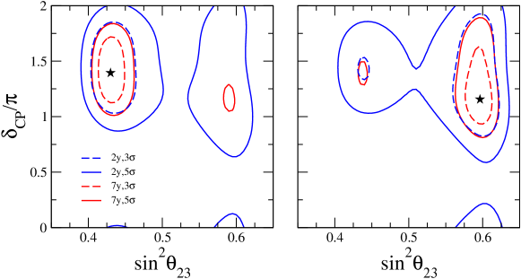
Figure 1: DUNE sensitivity projections for normal mass ordering of neutrinos, after 2 years (blue) and 7 years (red) run, taking the global best fit point (left panel) and the local minimum (right panel) of Ref. deSalas:2017kay as benchmark points (shown in star). The dashed lines represent $3\sigma$ and solid lines are for $5\sigma$ C.L. sensitivities.

As can be seen in the left panel of Fig. 1, if the true values of $\theta_{23}$ and $\delta_{CP}$ correspond to the current best fit value, then after only two years of running time, DUNE will be able to probe a large part of the parameter space at 3$\sigma$. After seven years of running time, the DUNE sensitivity will be much higher, so that at 3$\sigma$ C.L. it will rule out the possibility of $\theta_{23}$ being maximal, or lying in the upper octant. It will also rule out all possibilities of no CP violation in the lepton sector. At 5$\sigma$, apart from a very small parameter range, one finds that both the upper octant of $\theta_{23}$ as well as the CP conserving case will be ruled out. The maximal atmospheric angle can be ruled out at even higher confidence level.

On the other hand, for the current local minimum, after just two years of running DUNE will be able to rule out the lower octant solutions at 3$\sigma$ C.L. except for a small region of parameters, as can be seen in the right panel of Fig. 1. With seven years of running time, the allowed region in the $\theta_{23}-\delta_{CP}$ plane shrinks considerably, so that the left octant appears only at 5$\sigma$ C.L. The maximal value of $\theta_{23}$ will be ruled out at higher significance.

Since we currently do not know the mass ordering of neutrinos Gariazzo:2018pei , we have also examined the case of inverted ordering (IO). As in the previous case, for inverted ordering there are also two minima. The current data give a preferred minimum in the second octant, as well a local minimum in the first octant of $\theta_{23}$. The results of our DUNE simulation for these benchmark points are shown in Fig. 2.

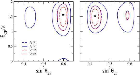
Figure 2: DUNE sensitivity projections for inverted mass ordering of neutrinos, after 2 years (blue) and 7 years (red) run, taking the global best fit point (left panel) and local minimum (right panel) of Ref. deSalas:2017kay as benchmark points (shown in star).

The left panel shows our DUNE simulation results for inverted mass ordering taking the global minimum as true value. After running for two years, most of the $\theta_{23}-\delta_{CP}$ plane, including maximal mixing and lower octant of $\theta_{23}$, would appear only at 5$\sigma$ C.L. Moreover, the CP conserving hypothesis will be disfavored at more than 5$\sigma$ after seven years running time. The right panel shows the results of our simulation for the IO case when we take the local minimum as true value. Again, DUNE measurements will considerably shrink the allowed region in the $\theta_{23}-\delta_{CP}$ plane. After two years of running time, CP conservation and maximal atmospheric mixing could be excluded beyond the 3$\sigma$ level, while only a very small region of parameters for the upper octant solution would survive. After seven years of running time, the upper octant solution would appear only at 5$\sigma$ C.L., while maximal atmospheric mixing and CP conservation would be ruled out beyond 5$\sigma$.

In short, should any of the current experimental benchmark points be the true value of neutrino oscillation parameters, then DUNE would exclude a very large part of the $\theta_{23}-\delta_{CP}$ plane, including opposite octant solutions, CP conserving scenarios as well as maximal mixing.

After taking a detailed look at the DUNE capabilities for experimentally motivated benchmark points, we now turn to the theoretically motivated scenarios. As mentioned before, one of the frequently occurring predictions in different models of leptonic mixing is the maximal mixing with CP conservation. There are two possible benchmark points corresponding to such a scenario, namely ($\sin^{2}\theta_{23}=0.5,\delta_{CP}=0$) and ($\sin^{2}\theta_{23}=0.5,\delta_{CP}=\pi$). We took these two points as our first theory motivated benchmark points for our DUNE simulations.

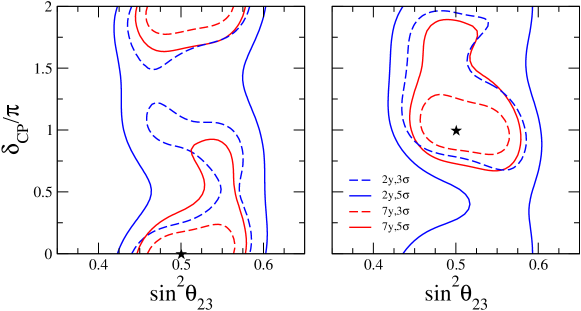
Figure 3: DUNE sensitivity projections expected after 2 years (blue) and 7 years (red) run, taking maximal mixing ($\sin^{2}\theta_{23}=0.5$) and no CP violation with $\delta_{CP}=0$ (left panel) and $\delta_{CP}=\pi$ (right panel) as benchmark points (star).

In the left panel of Fig. 3 we have taken ($\sin^{2}\theta_{23}=0.5,\delta_{CP}=0$) as the true value used to generate DUNE data. After two years of running time, the allowed region will shrink appreciably, particularly for $\theta_{23}$, although the maximal CP violation will still be allowed at 3$\sigma$ C.L. After seven years, the allowed region will shrink much further, so that maximal CP violation will be ruled out at 3$\sigma$ C.L, though a small parameter region will still remain allowed at 5$\sigma$. In the right panel of Fig. 3 we have taken the other CP conserving point, ($\sin^{2}\theta_{23}=0.5,\delta_{CP}=\pi$), as true value. With two years of running, DUNE will probe a large parameter region at 3$\sigma$ C.L., although maximal CP violation would be still allowed at that confidence level. After seven years of running time, however, the possibility of maximal CP violation would be excluded at 3$\sigma$, and the allowed region for $\theta_{23}$ will further shrink. At 5$\sigma$ C.L. only a small region for maximal CP violation would still survive.

Another theoretically well motivated case is the one of maximal atmospheric mixing and maximal CP violation. As in the previous case, two possibilities arise here, namely ($\sin^{2}\theta_{23}=0.5,\delta_{CP}=\pi/2$) and ($\sin^{2}\theta_{23}=0.5,\delta_{CP}=3\pi/2$). As our next example we have considered these two possibilities as true values, with the results shown in Fig. 4.

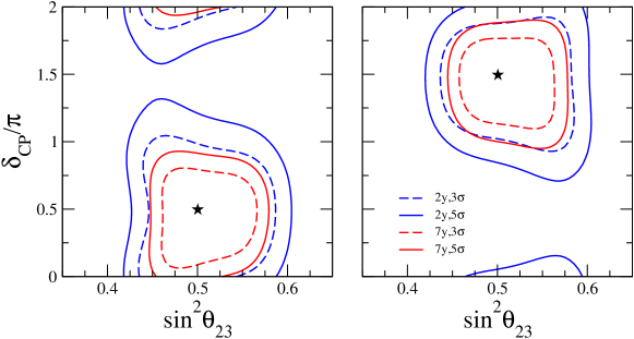
Figure 4: DUNE sensitivity projections expected after 2 years (blue) and 7 years (red) run, taking maximal mixing ($\sin^{2}\theta_{23}=0.5$) and maximal CP violation i.e. $\delta_{CP}=\pi/2$ (left) and $\delta_{CP}=3\pi/2$ (right panel) as benchmark points (star).

The left panel of Fig. 4 considers the former point as true value of the oscillation parameters, while the latter one has been considered in the right panel. In both cases, after two years of running time, the allowed region will shrink considerably. However, the possibility of CP conservation would remain allowed at 3$\sigma$. The situation improves significantly after analyzing seven years of DUNE running time. In that case, the CP conservation hypothesis would be completely excluded for both benchmark points at 3$\sigma$ C.L. At 5$\sigma$ only a small parameter region for CP conservation would survive in both cases.

As our final theory motivated benchmark point we examined the bi-large mixing scenario Boucenna:2012xb ; Ding:2012wh ; Roy:2014nua as the true value for our DUNE simulation. As explained before, this benchmark corresponds to $\sin^{2}\theta_{23}=0.45$. While the bi-large mixing ansatz in its simplest form does not predict any particular value of $\delta_{CP}$, here we have taken bi-large mixing without CP violation, $\delta_{CP}=0$, as our reference choice. The result of our simulation in this case is shown in Fig. 5.

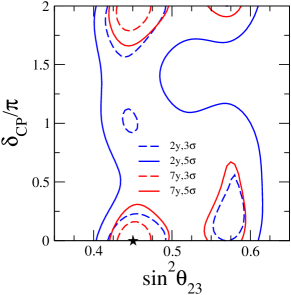
Figure 5: DUNE sensitivity projections expected after 2 years (blue) and 7 years (red) run, for the CP conserving bi-large mixing scenario ($\sin^{2}\theta_{23}=0.45$, $\delta_{CP}=0$) as our benchmark point (star).

Also here, as can be seen in the figure, after two years of DUNE data taking, the allowed parameter region will shrink considerably. However, the possibility of upper octant values of $\theta_{23}$ will still be allowed in some part of the parameter space at 3$\sigma$. As expected, after seven years of DUNE data taking, there will substantial improvement in the sensitivity to both parameters. Indeed, the upper octant solution for $\theta_{23}$ and maximal CP violating scenarios will be completely excluded at 3$\sigma$. At 5$\sigma$, maximal CP violation will only be allowed in a small region of upper octant values of $\theta_{23}$.

IV.2 Line Benchmarks

So far we have only considered benchmark points. In this section we consider more model-independent scenarios associated to line-like cases as possible true values in our simulations. The three line-like benchmark cases under study are:

1. Maximal atmospheric mixing ($\sin^{2}\theta_{23}=0.5$) for all possible values of $\delta_{CP}$.

2. CP conservation ($\delta_{CP}=0\,,\pi$) with arbitrary values of $\theta_{23}$.

3. Maximal CP violation ($\delta_{CP}=\pi/2\,,3\pi/2$) with arbitrary values of $\theta_{23}$.

As discussed in Sec. II, our first benchmark line occurs frequently in flavor models of leptonic mixing. The result of the simulation for this benchmark line is shown in Fig. 6.

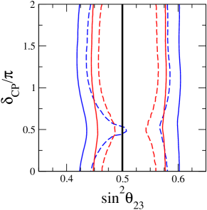
Figure 6: DUNE sensitivity projections after 2 years (blue) and 7 years (red) run, taking the maximal mixing ($\sin^{2}\theta_{23}=0.5$) scenario (arbitrary $\delta_{CP}$) as benchmark line (black).

As can be seen, after two years of running time, DUNE will considerably narrow down the currently allowed parameter range at both 3$\sigma$ and 5$\sigma$ C.L. After seven years of running time, the allowed region of parameter space for $\theta_{23}$ will shrink even further. Since in our simulations we have taken all possible values of $\delta_{CP}$ along the $\sin^{2}\theta_{23}=0.5$ line as true values, the information about the DUNE probing capabilities with respect to $\delta_{CP}$ is naturally lost in this simulation. Notice that the small kink in the 3$\sigma$ curve of our simulation for two year run around $\delta_{CP}=\pi/2$ is understood and reflects the fact that our simulations take into account the current experimental knowledge on these parameters which disfavors $\delta_{CP}\approx\pi/2$. As expected, after seven year of running time the kink is much less pronounced because at this point the corresponding curves for these parameters are totally driven by DUNE, hence the effect of the current global fit is washed out.

The next benchmark line we have examined is that corresponding to the CP conserving hypothesis, i.e., $\delta_{CP}=0$ or $\delta_{CP}=\pi$. We took these two values as benchmark lines for the rather conservative range of $\sin^{2}\theta_{23}\in[0.35,0.65]$, as mentioned in Tab. 3. The results for this case are shown in Fig. 7.

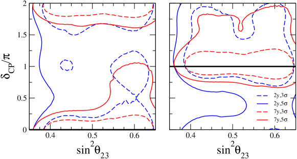
Figure 7: DUNE sensitivity projections expected after 2 years (blue) and 7 years (red) run, taking no CP violation cases $\delta_{CP}=0$ (left panel) and $\delta_{CP}=\pi$ (right panel) for arbitrary $\sin^{2}\theta_{23}$ as the benchmark lines (black).

As can be seen in the left panel, corresponding to $\delta_{CP}=0$, after just two years of data collection, DUNE can severely constrain the allowed range of $\delta_{CP}$ at 3$\sigma$ C.L. In fact, the possibility of maximal CP violation is almost ruled out at 3$\sigma$ C.L. After seven years of running time, the allowed region will shrink much more and DUNE would be able to exclude completely the possibility of maximal CP violation at 3$\sigma$ C.L. Even at 5$\sigma$ C.L., the allowed region after seven years of run would be significantly reduced and, apart from a small region, the possibility of maximal CP violation will be essentially excluded. The right panel of Fig. 7 shows the result of our simulation for $\delta_{CP}=\pi$. Again, after two years of DUNE running time, at 3$\sigma$ C.L. the allowed region $\delta_{CP}$ will shrink considerably. However, unlike in the previous case, here the possibility of maximal CP violation will still be allowed for most of the $\theta_{23}$ range. The root for this loss of discriminating power with respect to the previous case is the fact that the current global fit data prefers CP violation close to $\delta_{CP}\approx 3\pi/2$. Thus, in this case, our two year run DUNE simulations (which include the current global fit results) would not be able to rule out maximal CP violation. In contrast, however, after seven years of running time of DUNE, the simulation is mainly driven by the DUNE data sample that will be able to, not only further shrink the parameter space, but also rule out maximal CP violation at 3$\sigma$ C.L. Before moving on to next case, we would like to remark that, since we have taken the whole range of $\theta_{23}$ as true value for our benchmark lines, naturally the information about DUNE reach to $\theta_{23}$ is lost in this simulation. However, note that the extreme values of $\theta_{23}$ in both panels of Fig. 7 are indeed getting excluded in both two and seven year runs as these edge values are disfavored by current global fits at a very high significance.

As our final benchmark line, we have looked at the possibility of maximal CP violation. There are several theoretically motivated models that predict such a case. Also, the current experimental data indicates nearly maximal CP violation with $\delta_{CP}\approx 3\pi/2$. Again there are two possibilities for maximal CP violation namely $\delta_{CP}=\pi/2$ or $\delta_{CP}=3\pi/2$. We have taken these two values as our benchmark lines in the simulation for all allowed values of $\theta_{23}$ in the range $\sin^{2}\theta_{23}=[0.35,0.65]$. The result is shown in Fig. 8.

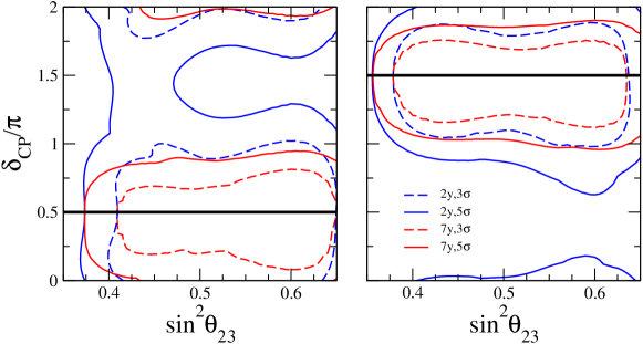
Figure 8: DUNE sensitivity projections expected after 2 years (blue) and 7 years (red) run, taking maximal CP violation cases $\delta_{CP}=\pi/2$ (left) and $\delta_{CP}=3\pi/2$ (right panel) for arbitrary $\sin^{2}\theta_{23}$ as the benchmark lines (black).

The left panel of this figure corresponds to the case of benchmark line $\delta_{CP}=\pi/2$. From the plot one can see that, after two years of running time of DUNE, the allowed values for $\delta_{CP}$ will shrink appreciably. However, the possibility of no CP violation will still be allowed for most values of $\theta_{23}$ at the 3$\sigma$ level. After seven years of running time the situation will drastically improve, and the CP conserving hypothesis could be ruled out at 3$\sigma$ C.L. The right panel of Fig. 8 shows the results for the benchmark line with $\delta_{CP}=3\pi/2$. In this case, after two years of running time, DUNE will be able to rule out the CP conserving scenario at 3$\sigma$ C.L. in the whole parameter range. Again, our results for two year simulations can be understood as arising from the fact that our simulations take into account the current experimental information on $\delta_{CP}$, as explained before. After seven years of running time, DUNE could considerably restrict the allowed range for $\delta_{CP}$, ruling out the CP conserving scenario at 5$\sigma$. As before, note that, since we have taken the whole range of $\sin^{2}\theta_{23}\in[0.35,0.65]$ as true value, the DUNE sensitivity on $\theta_{23}$ is not apparent in the simulations. However, as shown in both panels, the extreme end values of $\theta_{23}$, currently strongly disfavored by oscillation data, can be totally excluded at the 5$\sigma$ level.

A comment is in order concerning the benchmark line results, namely, the fact that in nature the true value of a given neutrino oscillation parameter will always correspond to a single point in parameter space. Nonetheless, the line-like simulations do carry useful information and can be used as a guide to narrow down the actual allowed range of these parameters. However, since in these simulations one takes all possible values of a given parameter lying on a line as true values, naturally the results of these simulations will not be as constraining as the results obtained in the previous section.

V Summary and discussion

Using the design specifications of the DUNE experiment and taking into account the current status of neutrino oscillation parameters, as summarized in global oscillation fits, we have determined DUNE’s potential to probe the pattern of neutrino mixing and CP violation after two and seven years of running. We have taken various input benchmark values as our true values. These include not only the current preferred values of $\theta_{23}$ and $\delta_{CP}$, as given in global oscillation fits, but also several theory-motivated choices as to what the true values of $\theta_{23}$ and $\delta_{CP}$ could be. We have examined quantitatively DUNE’s capability to probe deviations from maximality in the atmospheric angle $\theta_{23}$ and its octant, as well as to probe for the CP violation hypothesis itself, in a model-independent way. We have found that, after seven years of running, DUNE will be able to test quantitatively the predictions of various models of neutrino mixing. Our results are summarized in Figs. 1-8. They can be used so as to establish DUNE’s capability to discriminate between the various mixing scenarios analyzed above. Table 5, gives an “executive summary” of DUNE’s sensitivity to our various benchmark choices described in Sec. II.

	GM (NO)	LM (NO)	$\theta_{23}=45\degree$ $\delta_{CP}=0$	$\theta_{23}=45\degree$ $\delta_{CP}=\pi$	$\theta_{23}=45\degree$ $\delta_{CP}=\frac{\pi}{2}$	$\theta_{23}=45\degree$ $\delta_{CP}=\frac{3\pi}{2}$	Bi-large
GM (NO)	-	✓(✗)	✓(✓)	✓(✓)	✓(✓)	✓(✓)	✓(✓)
LM (NO)	✓(✗)	-	✓(✓)	✓(✓)	✓(✓)	✓(✓)	✓(✓)
$\theta_{23}=45\degree$ $\delta_{CP}=0$	✓(✓)	✓(✓)	-	✓(✓)	✓(✓)	✓(✓)	✓(✗)
$\theta_{23}=45\degree$ $\delta_{CP}=\pi$	✓(✓)	✓(✓)	✓(✓)	-	✓(✓)	✓(✗)	✓(✓)
$\theta_{23}=45\degree$ $\delta_{CP}=\frac{\pi}{2}$	✓(✓)	✓(✓)	✓(✗)	✓(✓)	-	✓(✓)	✓(✓)
$\theta_{23}=45\degree$ $\delta_{CP}=\frac{3\pi}{2}$	✓(✓)	✓(✓)	✓(✓)	✓(✗)	✓(✓)	-	✓(✓)
Bi-large	✓(✓)	✓(✓)	✓(✓)	✓(✓)	✓(✓)	✓(✓)	-

Table 5: The discriminating power of DUNE after running for seven years. Various mixing hypothesis, taken as true, are listed in the rows, while the columns indicate the mixing hypotheses that can be tested against the assumed true scenario. The convention for ticks and crosses is given in the text.

Each row in Tab. 5 corresponds to an assumed pair of parameters ($\theta_{23}$, $\delta_{CP}$), taken as true values, while the columns indicate the different mixing hypotheses that can be tested from the simulated DUNE data. The table corresponds to the results obtained for the case of normal mass ordering, from the simulation of seven years of future DUNE neutrino oscillation data, with a confidence level of 3$\sigma$ and 5$\sigma$ C.L. (in parentheses). Ticks and crosses mean that, assuming the true oscillation parameters as given in each row, the particular benchmark shown in every column can be ruled out at the given confidence, or not, respectively. For example, if we assume as true value for the oscillation parameters $\theta_{23}$ and $\delta_{CP}$ the ones given by the global minimum (GM) of the current oscillation fit (see Tab. 1), after seven years or run, DUNE will be able to exclude all the other analyzed mixing scenarios at 3$\sigma$ and 5$\sigma$ C.L., except for the local minimum (LM) benchmark point, that will be still compatible with data at the 5$\sigma$ level. Moreover, one sees that, with seven years of data, DUNE will have enough sensitivity to discriminate among all the benchmark points analyzed at 3$\sigma$ C.L., with only a few ambiguities remaining at the 5$\sigma$ level. In summary, one can conclude that DUNE will make a substantial step towards the precise determination of ($\theta_{23}$, $\delta_{CP}$), bringing to quantitative test the predictions of various theories of neutrino mixing.

- (1) T. Kajita, Nobel Lecture: Discovery of atmospheric neutrino oscillations, Rev. Mod. Phys. 88 (2016) 3 030501.
- (2) A. B. McDonald, Nobel Lecture: The Sudbury Neutrino Observatory: Observation of flavor change for solar neutrinos, Rev. Mod. Phys. 88 (2016) 3 030502.
- (3) P. F. de Salas et al., Status of neutrino oscillations 2017 (2017), arXiv:1708.01186 [hep-ph].
- (4) S. Morisi and J. W. F. Valle, Neutrino masses and mixing: a flavour symmetry roadmap, Fortsch.Phys. 61 466–492, arXiv:1206.6678 [hep-ph].
- (5) S. F. King et al., Neutrino Mass and Mixing: from Theory to Experiment, New J.Phys. 16 (2014) 045018, arXiv:1402.4271 [hep-ph].
- (6) P. F. Harrison, D. H. Perkins and W. G. Scott, Tri-bimaximal mixing and the neutrino oscillation data, Phys. Lett. B530 167.
- (7) K. S. Babu, E. Ma and J. W. F. Valle, Underlying A(4) symmetry for the neutrino mass matrix and the quark mixing matrix, Phys. Lett. B552 (2003) 207–213, arXiv:hep-ph/0206292 [hep-ph].
- (8) S. Morisi et al., Neutrino mixing with revamped A4 flavour symmetry, Phys.Rev. D88 016003, arXiv:1305.6774 [hep-ph].
- (9) S. S. Chatterjee et al., Cornering the revamped BMV model with neutrino oscillation data, Phys. Lett. B774 (2017) 179–182, arXiv:1708.03290 [hep-ph].
- (10) R. Acciarri et al. (DUNE), Long-Baseline Neutrino Facility (LBNF) and Deep Underground Neutrino Experiment (DUNE) (2016), arXiv:1601.02984 [physics.ins-det].
- (11) R. Acciarri et al. (DUNE), Long-Baseline Neutrino Facility (LBNF) and Deep Underground Neutrino Experiment (DUNE) Conceptual Design Report Volume 2: The Physics Program for DUNE at LBNF (2015), arXiv:1512.06148 [physics.ins-det].
- (12) P. F. Harrison and W. G. Scott, Symmetries and generalisations of tri-bimaximal neutrino mixing, Phys. Lett. B535 163–169, hep-ph/0203209.
- (13) G. Altarelli and F. Feruglio, Tri-bimaximal neutrino mixing, A(4) and the modular symmetry, Nucl. Phys. B741 (2006) 215–235, arXiv:hep-ph/0512103 [hep-ph].
- (14) E. Ma, Tribimaximal neutrino mixing from a supersymmetric model with A4 family symmetry, Phys. Rev. D73 (2006) 057304, arXiv:hep-ph/0511133 [hep-ph].
- (15) I. de Medeiros Varzielas, S. F. King and G. G. Ross, Tri-bimaximal neutrino mixing from discrete subgroups of SU(3) and SO(3) family symmetry, Phys. Lett. B644 (2007) 153–157, arXiv:hep-ph/0512313 [hep-ph].
- (16) W. Grimus and L. Lavoura, A non-standard CP transformation leading to maximal atmospheric neutrino mixing, Phys. Lett. B579 113–122, hep-ph/0305309.
- (17) A. Datta, F.-S. Ling and P. Ramond, Correlated hierarchy, Dirac masses and large mixing angles, Nucl.Phys. B671 383–400, arXiv:hep-ph/0306002 [hep-ph].
- (18) W. Rodejohann, Unified Parametrization for Quark and Lepton Mixing Angles, Phys. Lett. B671 (2009) 267–271, arXiv:0810.5239 [hep-ph].
- (19) E. Ma, Soft symmetry breaking and cobimaximal neutrino mixing, Phys. Lett. B755 (2016) 348–350, arXiv:1601.00138 [hep-ph].
- (20) E. Ma, Cobimaximal neutrino mixing from , Phys. Lett. B777 (2018) 332–334, arXiv:1707.03352 [hep-ph].
- (21) E. Ma and G. Rajasekaran, Cobimaximal neutrino mixing from and its possible deviation, EPL 119 (2017) 3 31001, arXiv:1708.02208 [hep-ph].
- (22) S. Gariazzo et al., Neutrino masses and their ordering: Global Data, Priors and Models (2018), arXiv:1801.04946 [hep-ph].
- (23) F. P. An et al. (Daya Bay), Measurement of electron antineutrino oscillation based on 1230 days of operation of the Daya Bay experiment (2016), arXiv:1610.04802 .
- (24) M. Y. Pac (RENO), Recent Results from RENO (2018) arXiv:1801.04049 , URL http://inspirehep.net/record/1647948/files/arXiv:1801.04049.pdf.
- (25) Y. Abe et al. (Double Chooz), Improved measurements of the neutrino mixing angle with the Double Chooz detector, JHEP 10 (2014) 086, [Erratum: JHEP02,074(2015)], arXiv:1406.7763.
- (26) S. Boucenna et al., Bi-large neutrino mixing and the Cabibbo angle, Phys.Rev. D86 051301, arXiv:1206.2555 [hep-ph].
- (27) G.-J. Ding, S. Morisi and J. W. F. Valle, Bi-large Neutrino Mixing and Abelian Flavor Symmetry, Phys.Rev. D87,053013, arXiv:1211.6506 [hep-ph].
- (28) S. Roy et al., The Cabibbo angle as a universal seed for quark and lepton mixings, Phys. Lett. B748 (2015) 1–4, arXiv:1410.3658 [hep-ph].
- (29) J. Schechter and J. W. F. Valle, Neutrino Masses in SU(2) x U(1) Theories, Phys. Rev. D22 (1980) 2227.
- (30) P. Chen et al., Warped flavor symmetry predictions for neutrino physics, JHEP 01 (2016) 007, arXiv:1509.06683 [hep-ph].
- (31) P. Chen et al., Generalized reflection symmetry and leptonic CP violation, Phys. Lett. B753 (2016) 644–652, arXiv:1512.01551 [hep-ph].
- (32) A. E. Carcamo Hernandez et al., Predictive Pati-Salam theory of fermion masses and mixing, JHEP 07 (2017) 118, arXiv:1705.06320 [hep-ph].
- (33) S. Centelles Chuliá, R. Srivastava and J. W. F. Valle, Generalized Bottom-Tau unification, neutrino oscillations and dark matter: predictions from a lepton quarticity flavor approach, Phys. Lett. B773 (2017) 26–33, arXiv:1706.00210 [hep-ph].
- (34) C. Bonilla, et al Flavour-symmetric type-II Dirac neutrino seesaw mechanism (2017), arXiv:1710.06498 [hep-ph].
- (35) P. Pasquini, S. C. Chuliá and J. W. F. Valle, Neutrino oscillations from warped flavor symmetry: predictions for long baseline experiments T2K, NOvA and DUNE, Phys. Rev. D95 (2017) 9 095030, arXiv:1610.05962 [hep-ph].
- (36) S. S. Chatterjee, P. Pasquini and J. W. F. Valle, Probing atmospheric mixing and leptonic CP violation in current and future long baseline oscillation experiments, Phys. Lett. B771 (2017) 524–531, arXiv:1702.03160 [hep-ph].
- (37) R. Srivastava, et. al, Testing a lepton quarticity flavor theory of neutrino oscillations with the DUNE experiment (2017), arXiv:1711.10318 [hep-ph].
- (38) K. Abe et al. (T2K), Updated T2K measurements of muon neutrino and antineutrino disappearance using 1.51021 protons on target, Phys. Rev. D96 (2017) 1 011102, arXiv:1704.06409 [hep-ex].
- (39) K. Abe et al. (T2K), Combined Analysis of Neutrino and Antineutrino Oscillations at T2K, Phys. Rev. Lett. 118 (2017) 15 151801, arXiv:1701.00432 [hep-ex].
- (40) P. Adamson et al. (NOvA), Measurement of the neutrino mixing angle in NOvA, Phys. Rev. Lett. 118 (2017) 15 151802, arXiv:1701.05891 .
- (41) P. Adamson et al. (NOvA), Constraints on Oscillation Parameters from Appearance and Disappearance in NOvA, Phys. Rev. Lett. 118 (2017) 23 231801, arXiv:1703.03328 .
- (42) P. Huber, M. Lindner and W. Winter, Simulation of long-baseline neutrino oscillation experiments with GLoBES (General Long Baseline Experiment Simulator), Comput. Phys. Commun. 167 (2005) 195, arXiv:hep-ph/0407333 [hep-ph].
- (43) P. Huber et al., New features in the simulation of neutrino oscillation experiments with GLoBES 3.0: General Long Baseline Experiment Simulator, Comput. Phys. Commun. 177 (2007) 432–438, arXiv:hep-ph/0701187 [hep-ph].
- (44) T. Alion et al. (DUNE), Experiment Simulation Configurations Used in DUNE CDR (2016), arXiv:1606.09550 [physics.ins-det].