Seeking leptoquarks in IceCube

Abstract

We investigate the sensitivity of IceCube(-Gen2) to a scalar leptoquark scenario with couplings only to heavy quark flavors which may be connected to solving discrepancies in $B$-meson semileptonic decays. We take into account, for the first time, the non-negligible neutrino-gluon cross section induced by leptoquarks, and we systematically account for indirect and direct constraints which have been overlooked in previous studies. We conclude that IceCube(-Gen2) can only probe the light LQ regime, already disfavored by the combination of flavor physics constraints, electroweak precision data and the direct searches at the LHC.

LPT-Orsay-18-42

1 Introduction

It is remarkable that the two types of constituents in the flavor sector of the Standard Model (SM), quarks and leptons, although independent, share a number of common features. They come in three generations that conspire to exactly cancel the triangle anomalies of the gauge interactions, they exhibit mixing between mass and flavor eigenstates resulting in oscillations, and flavor changing neutral interactions do not occur at tree-level. These common features strongly suggest that quarks and leptons should be somehow interrelated. In fact, leptoquarks (LQs), bosons that can mediate quark-lepton transitions, appear in many extensions of the SM, in particular, in Grand Unified Theories Georgi:1974sy ; Pati:1974yy , and composite Higgs models Abbott:1981re ; Schrempp:1984nj ; Wudka:1985ef .

From a phenomenological point of view, LQs are $SU(3)_{c}$ colored particles that can come as $SU(2)_{L}$ singlets, doublets or triplets Buchmuller:1986zs ; Dorsner:2016wpm . Their masses, strength and flavor structure of their couplings to quarks and leptons are all undetermined when the ultraviolet completion is unknown. Since LQs with masses of the order of the electroweak scale are not disallowed by any fundamental reason, it is important to look for them in all possible ways. In fact, many collider experiments have been searching for them in pair as well as in single production modes. From HERA to the LHC, experiments have been setting stringent limits on their masses and couplings, c.f. Aktas:2005pr ; Diaz:2017lit and references therein. These limits depend, unfortunately, unavoidably on the assumed flavor structure, some of which are difficult to explore in accelerators. Other bounds deduced from the direct searches have been discussed in Ref. Greljo:2017vvb , see also references therein.

Besides the purely theoretical reasons that compel experimentalists to look for these particles it seems there might be an experimental one too, coming from $B$-physics. The excellent agreement between the SM predictions and experimental data seems to be disrupted by flavor physics. Recent data from the LHC, Belle and BaBar suggest lepton flavor universality violation (LFUV) in $B$-meson semileptonic decays. The LHCb experiment, for instance, has reported about 2.6$\sigma$ discrepancy in the ratio of the partial branching fractions of the loop induced transitions (denoted by $\mathcal{B}^{\prime}$),

$$R_{K^{(\ast)}}^{\rm exp}=\frac{{\cal B}^{\prime}(B\to K^{(\ast)}\mu^{+}\mu^{-})}{{\cal B}^{\prime}(B\to K^{(\ast)}e^{+}e^{-})}\,,$$ (1)

and the measured values Aaij:2014ora ; Aaij:2017vbb appear to be smaller than predicted in the SM Hiller:2003js ; Bordone:2016gaq . Another intriguing indication of LFUV comes from the tree-level ratio Amhis:2016xyh

$$R_{D}^{\rm exp}=\frac{{\cal B}(B\to D\tau\nu)}{{\cal B}(B\to D\ell\nu)}=0.41\pm 0.05\,,$$ (2)

where $\ell=e,\mu$, obtained by combining Babar and Belle results Lees:2012xj ; Huschle:2015rga ; Sato:2016svk ; Aaij:2015yra ; Hirose:2016wfn and 2.2$\sigma$ above $R_{D}^{\rm SM}=0.300(8)$, the SM prediction Amhis:2016xyh ; Na:2015kha ; Lattice:2015rga . This feature was confirmed with $R_{D^{\ast}}^{\rm exp}=0.304(15)$ Lees:2012xj ; Huschle:2015rga ; Aaij:2017deq , which also appears about 3$\sigma$ larger than the SM prediction, $R_{D^{\ast}}^{\rm SM}=0.260(8)$ Fajfer:2012vx ; Bigi:2017jbd . Another confirmation of this phenomenon was reported by LHCb who measured $R_{J/\psi}={\cal B}(B_{c}\to J/\psi\tau\nu)/{\cal B}(B_{c}\to J/\psi\mu\nu)=0.71\pm 0.25$ Aaij:2017tyk , also larger than the SM estimates although the SM value in this case is less reliable. Many proposed solutions to these anomalies discussed in the literature so far rely on existence of LQ states Hiller:2014yaa ; Ghosh:2014awa ; Alonso:2015sja ; Fajfer:2015ycq ; Barbieri:2015yvd ; Bauer:2015knc ; Deppisch:2016qqd ; Arnan:2016cpy ; Becirevic:2016yqi ; Cox:2016epl ; Hiller:2016kry ; Dorsner:2017ufx ; Barbieri:2016las ; Becirevic:2017jtw ; Fajfer:2018bfj ; Cai:2017wry ; Aloni:2017ixa ; Crivellin:2017dsk ; Crivellin:2017zlb ; Buttazzo:2017ixm ; DiLuzio:2017vat ; Calibbi:2017qbu ; Bordone:2017bld ; Barbieri:2017tuq ; DiLuzio:2017fdq ; Cline:2017aed ; Blanke:2018sro ; Assad:2017iib , notice that similar solutions can be implemented by considering supersymmetric models including R-Parity violating squarks Altmannshofer:2017poe . The couplings of LQs to heavy quarks can be as peculiar as to make them difficult for direct observations in colliders and it is therefore useful to try and look for them in other ways.

Here we study a possibility of using the IceCube neutrino telescope in the South Pole as a complementary way to search for those states. Many authors have explored the potential of IceCube to test LQ models, in particular, after the observation of an excess of high energy stating events consistent with a flux of high-energy astrophysical neutrinos from outside our galaxy Aartsen:2013jdh . In Ref. Anchordoqui:2006wc electroweak singlet LQ that couple to either second or third generation of quarks and/or leptons were studied, emphasizing the use of the inelasticity distribution of events to improve background rejection. Refs. Barger:2013pla , Dutta:2015dka and Mileo:2016zeo evoke LQ couplings to the first generation of quarks and leptons in order to try to accommodate IceCube high-energy neutrino data. Similarly, in Dev:2016uxj a supersymmetric model including R-parity violating squark resonances is considered to explain IceCube data. The limits that IceCube data can impose on a specific low-scale quark-lepton unification model with scalar LQs was studied in Dey:2015eaa . Scalar LQ doublets that couple the first and third family of quarks to leptons, with a flavor structure that can address the anomalies in $R_{K^{(\ast)}}$, pass other LHC constraints and give a sizable contribution to IceCube neutrino data were considered in Chauhan:2017ndd and by a more elaborated analysis in Dey:2017ede . The LQ states in all of these works, with exception of Ref. Anchordoqui:2006wc , couple to the first generation of quarks. Couplings to the first generation suffer, however, from severe experimental constraints as they have to comply with limits from direct searches at colliders, atomic parity violation experiments and flavor physics observables in the kaon/pion sectors. Moreover, all previous studies of the neutrino-nucleon cross-section at IceCube only consider the resonant $s$- and $t$-channel interactions of high energy neutrinos with quarks (valence and/or sea) via a LQ exchange. Nonetheless, we should not forget that in order to compute neutrino-nucleon cross sections we must also include the neutrino interaction with gluons mediated by a LQ, particularly important in accessing LQs that only couple to heavy quarks. Those are, in fact, the kinds of LQs that can take part in solving the discrepancies between data and heavy meson semileptonic decays. In this paper, we include for the first time the neutrino-gluon cross-section in order to consistently study the sensitivity of IceCube to LQ scenarios. Furthermore, we systematically compare the future IceCube future sensitivity with the indirect constraints coming from flavor physics and $Z$-pole observables, as well as the direct limits from the LHC, which are very efficient in constraining the LQ couplings.

Our paper is organized as follows. In Sec. 2 we describe a LQ model with a particular simple flavor structure that can solve $R_{D^{(\ast)}}$ and give rise to new neutrino-nucleon interactions which can be probed by IceCube. Furthermore, we perform a complete study of the indirect bounds on LQ couplings stemming from flavor physics and $Z$-pole observables. In Sec. 3 we review the High Energy Starting Events sample collected by IceCube after six years and we discuss the current status of the SM fit. We explain the procedure to simulate both the SM and LQ events at IceCube in order to compare with experimental data. In Sec. 4 we present results of our analysis and discuss what we can learn about our model from six years of IceCube data as well as the prospects for what can be expected in the future. We finally conclude in Sec. 5. All LQ contributions to the neutrino-nucleon scattering cross section, including the new ones, are collected in Appendix A, while in Appendix B we describe the transport equation for Earth’s attenuation. The decay rate expressions for $B\to D\ell\bar{\nu}$ are provided in Appendix C.

2 A Simple Leptoquark Scenario to Explain $R_{D^{(\ast)}}$

In this paper we focus on the so called $R_{2}$-model which involves an electroweak doublet of scalar LQs with hypercharge $Y=7/6$, described by the Yukawa Lagrangian,

$$\begin{split}\mathcal{L}_{\Delta^{(7/6)}}&=(g_{R})_{ij}\bar{Q}_{i}{\boldsymbol{\Delta}}^{(7/6)}\ell_{Rj}+(g_{L})_{ij}\bar{u}_{Ri}{\widetilde{\boldsymbol{\Delta}}}^{(7/6)\dagger}L_{j}+\mathrm{h.c.}\\[8.61108pt] &=(Vg_{R})_{ij}\bar{u}_{i}P_{R}\ell_{j}\,\Delta^{(5/3)}+(g_{R})_{ij}\bar{d}_{i}P_{R}\ell_{j}\,\Delta^{(2/3)}\\[5.59721pt] &\quad+(g_{L}U)_{ij}\bar{u}_{i}P_{L}\nu_{j}\,\Delta^{(2/3)}-(g_{L})_{ij}\bar{u}_{i}P_{L}\ell_{j}\,\Delta^{(5/3)}+\mathrm{h.c.},\end{split}$$ (3)

where in the first line the Lagrangian is given in the flavor basis and the superscripts in the LQ fields refer to the hypercharge ($Y$), while in the other two lines the Lagrangian is given in the mass eigenstate basis in which the superscripts of LQs refer to the electric charge $Q=Y+T_{3}$, where $Y$ is the hypercharge and $T_{3}$ the third component of weak isospin. Note that ${\widetilde{\mathbb{\Delta}}}=i\tau_{2}\mathbb{\Delta}^{\ast}$ is the conjugate of the doublet of mass degenerate LQs, while $V$ and $U$ stand for the Cabibbo-Kobayashi-Maskawa (CKM) and the Pontecorvo-Maki-Nakagawa-Sakata (PMNS) matrices, respectively. Furthermore, $P_{L,R}=(1\mp\gamma_{5})/2$ are the chiral projectors, $Q_{i}=[(V^{\dagger}u_{L})_{i}\;d_{Li}]^{T}$ and $L_{i}=[(U\nu_{L})_{i}\;\ell_{Li}]^{T}$ denote quark and lepton SU(2)_L doublets, whereas $u_{L}$, $d_{L}$, $\ell_{L}$ and $\nu_{L}$ are the fermion mass eigenstates.

We opt for the minimalistic structure of the Yukawa coupling matrices $g_{L,R}$ and assume

$$g_{L}=\left(\begin{matrix}0&0&0\\ 0&0&g_{L}^{c\tau}\\ 0&0&0\end{matrix}\right),\qquad g_{R}=\left(\begin{matrix}0&0&0\\ 0&0&0\\ 0&0&g_{R}^{b\tau}\end{matrix}\right),\qquad Vg_{R}=\left(\begin{matrix}0&0&V_{ub}g_{R}^{b\tau}\\ 0&0&V_{cb}g_{R}^{b\tau}\\ 0&0&V_{tb}g_{R}^{b\tau}\end{matrix}\right),$$ (4)

that allows $\Delta^{(2/3)}$ to mediate a tree-level contribution to $R_{D^{(\ast)}}$ and generates a contribution to the neutrino-nucleon scattering in IceCube.

2.1 $R_{2}$ explanation of $R_{D^{(\ast)}}$

In order to confront the LQ contributions with the experimental data involving the $B\to D\tau\nu$ decay we consider the effective Hamiltonian

$$\begin{split}{\cal H_{\mathrm{eff}}}=\frac{4\,G_{F}}{\sqrt{2}}V_{cb}\bigg{[}(\bar{\tau}_{L}\gamma^{\mu}\nu_{L})(\bar{c}_{L}\gamma_{\mu}b_{L})&+g_{S}(\mu)\,(\bar{\tau}_{R}\nu_{L})(\bar{c}_{R}b_{L})\\[0.50003pt] &+g_{T}(\mu)\,(\bar{\tau}_{R}\sigma^{\mu\nu}\nu_{L})(\bar{c}_{R}\sigma_{\mu\nu}b_{L})\bigg{]}+\mathrm{h.c.}\,,\end{split}$$ (5)

where $g_{S,T}$ are the Wilson coefficients induced by the LQ state mediating the semileptonic decay via a tree-level contribution shown in Fig. 1. After integrating out $\Delta^{(2/3)}$, the expression for $g_{S,T}$, at the matching scale $\mu=m_{\Delta}$, reads:

$$g_{S}(\mu=m_{\Delta})=4\,g_{T}(\mu=m_{\Delta})=\frac{g_{L}^{c\tau}\,\left(g_{R}^{b\tau}\right)^{\ast}}{4\sqrt{2}\,m_{\Delta}^{2}\,G_{F}V_{cb}}\,,$$ (6)

clearly enhanced by $V_{cb}^{-1}$. By virtue of the leading order QCD running from $\mu=m_{\Delta}\approx 1$ TeV down to $\mu=m_{b}$, the above relation between $g_{S}$ and $g_{T}$ becomes

$$g_{S}(\mu=m_{b})\approx 7.2\times g_{T}(\mu=m_{b})\,.$$ (7)

Furthermore, we included the small electroweak corrections discussed in Ref. Gonzalez-Alonso:2017iyc which can induce mixing between the scalar and tensor contributions.

Figure 1: Contribution to $b\to c\tau\bar{\nu}_{\tau}$ arising from the LQ model discussed in this paper. $\Delta\equiv\Delta^{(2/3)}$ stands for the LQ.

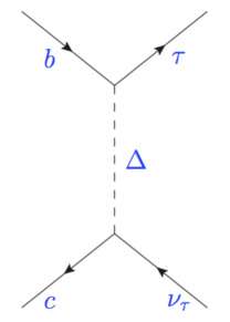
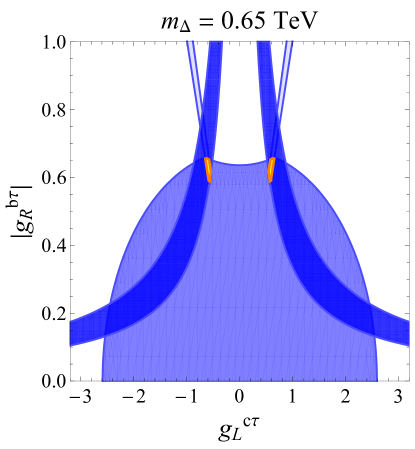
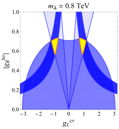
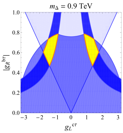
We focus on $B\to D$ semileptonic decays for which the hadronic form factors have been computed by means of numerical simulations of QCD on the lattice in Refs. Na:2015kha ; Lattice:2015rga .  To fill the discrepancy between $R_{D}^{\rm SM}$ and $R_{D}^{\rm exp}$ one then allows for $g_{S}\neq 0$. In this way we find the region of allowed values of $\mathrm{Re}[g_{S}(m_{b})]$ and $\mathrm{Im}[g_{S}(m_{b})]$ which is depicted by the blue regions in Fig. 2 to $1$, $2$ and $3\sigma$ accuracy.

Figure 2: Regions of allowed values for $g_{S}(\mu=m_{b})$ on the complex plane, compatible with experimentally measured $R_{D}$ to $1-$, $2-$ and $3\sigma$ (from darker to lighter blue). We assumed $g_{S}(\mu=m_{\Delta})=4\times g_{T}(\mu=m_{\Delta})$, as predicted by the $R_{2}$ LQ scenario, and considered the QCD running from $\mu\approx 1~{}\mathrm{TeV}$ to $m_{b}$, cf. Eq. (7). We also show in black the region compatible to $2\sigma$ accuracy with $R_{D^{\ast}}^{\mathrm{exp}}$, which indicates that the effective couplings must be complex in this scenario. See discussion in the text.

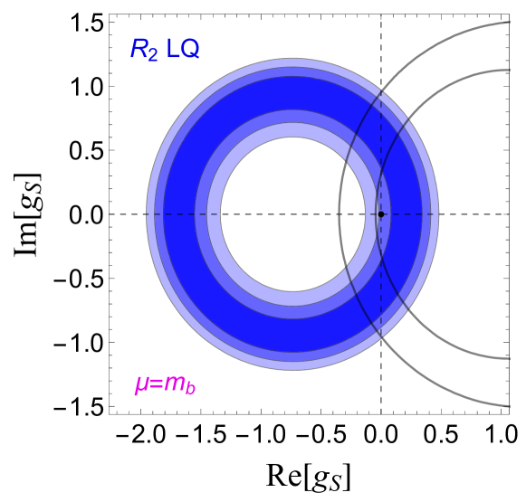
We decided not to include $R_{D^{\ast}}$ in the same fit because the lattice QCD determination of the form factors at non-zero recoil has not been made, in addition to the fact that the relevant pseudoscalar form factor has never been computed on the lattice. To verify that our solution to $R_{D}$ also gives an improvement of $R_{D^{\ast}}$, despite the uncertainties mentioned above which need to be clarified by lattice simulations, we show in the same plot the $2\sigma$ region consistent with $R_{D^{\ast}}^{\mathrm{exp}}$. The latter region was obtained by using the $B\to D^{\ast}\ell\nu_{\ell}$ form factors extracted from experimental results Amhis:2016xyh , combined with the ratio $A_{0}(q^{2})/A_{1}(q^{2})$ and $T_{1-3}(q^{2})/A_{1}(q^{2})$ computed in Ref. Bernlochner:2017jka . By using this approach, we conclude that, in the $R_{2}$-model, only the complex $g_{S}$ solutions to $R_{D}$ can provide a reasonable agreement with $R_{D^{(\ast)}}^{\rm exp}$, a fact that agrees with findings of Ref. Sakaki:2013bfa . Therefore, we will focus our analysis on the solutions to $R_{D}$ with complex Wilson coefficients

$$|g_{S}(\mu=m_{b})|\in(0.56,0.74)\,,$$ (8)

obtained to $1\sigma$ accuracy. This relation implies that the magnitude of LQ couplings should be such that

$$\dfrac{|g_{L}^{c\tau}||g_{R}^{b\tau}|}{m_{\Delta}^{2}}\in(0.80,1.32)\times(1~{}\mathrm{TeV})^{-2}\,,$$ (9)

where we used $|V_{cb}|=0.0417(20)$ Bona:2006ah . We see that the couplings needed to explain $R_{D}$ for $m_{\Delta}\lesssim 1~{}\mathrm{TeV}$ should not be too large, mostly due to the CKM enhancement in Eq. (6).

In the following we show that the explanation of $R_{D^{(\ast)}}^{\mathrm{exp}}>R_{D^{(\ast)}}^{\mathrm{SM}}$ described above is consistent with other limits from flavor physics and the direct searches for pair-produced LQs at the LHC. To that purpose, we will assume that the coupling $g_{R}^{b\tau}$ is purely imaginary.

2.2 General Constraints

The choice of $g_{L}^{c\tau}\neq 0$ and $g_{R}^{b\tau}\neq 0$ in Eq. (4) allows us to avoid many flavor physics constraints, making this explanation of $R_{D^{(\ast)}}^{\mathrm{exp}}>R_{D^{(\ast)}}^{\mathrm{SM}}$ particularly simple. Processes mediated by the flavor-changing neutral $\Delta F=1$ and $\Delta F=2$ currents are not altered in this scenario. Only the charged-current transitions $b\to c\tau\bar{\nu}$ are modified, as desired. The most significant constraints to this scenario actually come from the $Z$ boson decay widths.

2.2.1 Constraints from $Z$ decays

Our LQ model induces modifications to $Z$-boson decays through loop contributions, as depicted in Fig. 3. Those effects have to be consistent with the LEP measurements of $\mathcal{B}(Z\to\ell^{+}\ell^{-})$ Patrignani:2016xqp . The Lagrangian describing the $Zf\bar{f}$ coupling can be written as

$${\cal L}_{Zf\bar{f}}=\frac{g}{\cos\theta_{W}}Z^{\mu}\bar{f}\gamma_{\mu}\left(g_{L}^{f}\,P_{L}+g_{R}^{f}\,P_{R}\right)f\,,$$ (10)

where $g$ is the $SU(2)_{L}$ gauge coupling, and

$$\begin{split}g_{L}^{f}&=g_{L}^{f,\,\mathrm{SM}}+\delta g_{L}^{f}\,,\\ g_{R}^{f}&=g_{R}^{f,\,\mathrm{SM}}+\delta g_{R}^{f}\,,\end{split}$$ (11)

where $g_{L}^{f,\,\mathrm{SM}}=T_{3}-Q\sin^{2}\theta_{W}$ and $g_{R}^{f,\,\mathrm{SM}}=-Q\sin^{2}\theta_{W}$ are the SM contributions, while $\delta g_{L,R}^{f}$ parametrize LQ loop contributions. The corresponding branching ratio is then given by

$$\begin{split}{\cal B}(Z\to f\bar{f})=\frac{m_{Z}^{3}}{6\pi v^{2}\Gamma_{Z}}\,\beta_{f}&\,\left[\left[\big{|}g_{L}^{f}\big{|}^{2}+\big{|}g_{R}^{f}\big{|}^{2}\right]\left(1-\dfrac{m_{f}^{2}}{m_{Z}^{2}}\right)+\dfrac{6m_{f}^{2}}{m_{Z}^{2}}\mathrm{Re}\left(g_{L}^{f}\,g_{R}^{f\ast}\right)\,\right],\end{split}$$ (12)

where $m_{f}$ is the fermion mass and $\beta_{f}=\sqrt{1-4m_{f}^{2}/m_{Z}^{2}}$.

Figure 3: Contributions to the $Z\to f\bar{f}$ decay amplitude generated in our $R_{2}$ model, where the LQ $\Delta$ is either $\Delta^{(2/3)}$ or $\Delta^{(5/3)}$, $q\in\{u,c,b,t\}$ depending on the LQ state running in the loop, while $f$ is either $\ell$ or $\nu$. Similar diagrams can be drawn for $Z\to b\bar{b}$.

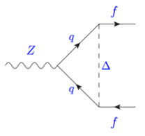
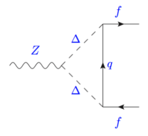
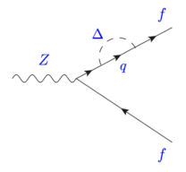
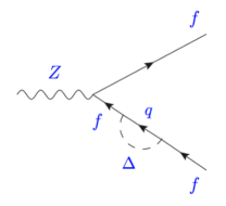
The LQ couplings lead to up- and down-type quark loop contributions to $\delta g_{L(R)}^{\tau}$, which are given by

$$\begin{split}\delta g_{R}^{\tau}&=N_{c}\,|g_{R}^{b\tau}|^{2}\Bigg{\{}|V_{tb}|^{2}\,\frac{x_{t}}{32\pi^{2}}\left(1+\log x_{t}\right)\\ &+\dfrac{x_{z}}{144\pi^{2}}\Bigg{[}-\left((\sin^{2}\theta_{W}-\dfrac{3}{2}\right)\left(\log x_{z}+i\pi\right)+\left(-\dfrac{1}{4}+\dfrac{2}{3}\sin^{2}\theta_{W}\right)\Bigg{]}\\ &+(1-|V_{tb}|^{2})\,\dfrac{x_{z}}{72\pi^{2}}\Bigg{[}\left(\sin^{2}\theta_{W}-\frac{3}{4}\right)\left(\log x_{z}+i\pi+\dfrac{1}{12}\right)+\dfrac{3}{16}\Bigg{]}\Bigg{\}}\,,\end{split}$$ (13)

and

$$\begin{split}\delta g_{L}^{\tau}&=N_{c}\,|g_{L}^{c\tau}|^{2}\dfrac{x_{z}}{72\pi^{2}}\Bigg{[}\sin^{2}\theta_{W}\left(\log x_{z}+i\pi+\dfrac{1}{12}\right)-\dfrac{1}{8}\Bigg{]},\end{split}$$ (14)

where $x_{t}=m^{2}_{t}/m^{2}_{\Delta}$ and $x_{z}=m^{2}_{Z}/m^{2}_{\Delta}$, and $N_{c}=3$ is the number of colors.  The dominant term in $\delta g_{R}^{\tau}$ comes from the top quark since it enhances the loop function. The effective coupling $\delta g_{L}^{\tau}$ does not exhibit a similar mass enhancement, and it is for this reason less relevant for phenomenology. Similarly, the LQ interaction with the charm quarks also induces an effective coupling to $\tau$ neutrinos, which reads

$$\delta g_{L}^{\nu_{\tau}}=N_{c}\,|g_{L}^{c\tau}|^{2}\dfrac{x_{z}}{72\pi^{2}}\Bigg{[}\sin^{2}\theta_{W}\left(\log x_{z}+i\pi-\dfrac{1}{6}\right)+\dfrac{1}{8}\Bigg{]}\,.$$ (15)

The effective couplings given above are constrained by the LEP measurements of the $Z$ decay widths and other electroweak observables Patrignani:2016xqp . The measurements of the effective $Z$ couplings give ALEPH:2005ab ,

$$\dfrac{g_{V}^{\tau}}{g_{V}^{e}}=0.959(29)\,,\qquad\quad\qquad\dfrac{g_{A}^{\tau}}{g_{A}^{e}}=1.0019(15)\,,$$ (16)

where $g_{V(A)}^{f}=g_{L}^{f}\pm g_{R}^{f}$. These results translate into useful bounds on the LQ contributions to $\delta g_{L,R}^{\tau}$. Furthermore, the LEP bound on the effective number of neutrinos ALEPH:2005ab

$$N_{\nu}=2.9840(82)\,,$$ (17)

will constrain the LQ couplings via the expression,

$$N_{\nu}=2+\left|1+\dfrac{\delta g_{L}^{\nu_{\tau}}}{g_{L}^{\nu_{\tau},\,\mathrm{SM}}}\right|^{2}\,.$$ (18)

As we shall see below, the coupling $g_{R}^{b\tau}$ is tightly limited by $\mathcal{B}(Z\to\tau\tau)$ due to the enhancement of the loop function by the top quark mass. On the other hand, the constraints on $g_{L}^{c\tau}$ derived from $N_{\nu}$ would be relevant only for very light LQ states, already excluded by the constraints stemming from $g_{V,A}^{\tau}$. Finally, we have also checked that the bound on the LQ couplings arising from $\mathcal{B}(Z\to b\bar{b})$ is not significant with current experimental precision.

2.2.2 Limits from Direct Detection

Direct searches at the LHC for pair-produced LQs provide useful limits on the couplings $g_{L}^{c\tau}$ and $g_{R}^{b\tau}$ as a function of the LQ mass $m_{\Delta}$. For the flavor ansatz given in Eq. (4) the allowed LQ decay modes are

$$\begin{split}\Delta^{(2/3)}&\to c\nu,~{}b\tau\,,\\ \Delta^{(5/3)}&\to u\tau,~{}c\tau,~{}t\tau\,.\end{split}$$ (19)

The CMS collaboration recently improved bounds of LQs decaying to $b\tau$, obtaining a lower bound on $m_{\Delta}$ of $900$ GeV, with the assumption ${\cal B}(\Delta^{(2/3)}\to b\tau)=1$ Khachatryan:2016jqo ; CMS:2016hsa . Similarly, CMS excludes LQs decaying into $t\tau$ with masses $m_{\Delta}\gtrsim 850~{}\mathrm{GeV}$ if $\mathcal{B}(\Delta^{(5/3)}\to t\tau)=1$ Khachatryan:2015bsa ; Sirunyan:2018nkj . Furthermore, a search for pair-produced LQs decaying into a light quark ($q=u,d,s,c$) and a neutrino has been reported by CMS, allowing us to set the limit $m_{\Delta}\gtrsim 980$ GeV if $\mathcal{B}(\Delta^{(2/3)}\to c\nu)=1$ CMS:2018bhq .

Figure 4: Exclusion regions of $m_{\Delta}$ as a function of $\mathcal{B}(\Delta^{(2/3)}\to b\tau)$ Khachatryan:2016jqo ; CMS:2016hsa , $\mathcal{B}(\Delta^{(5/3)}\to t\tau)$ Khachatryan:2015bsa ; Sirunyan:2018nkj and $\mathcal{B}(\Delta^{(2/3)}\to c\nu)$ CMS:2018bhq at $95\%$ CL. See text for details.

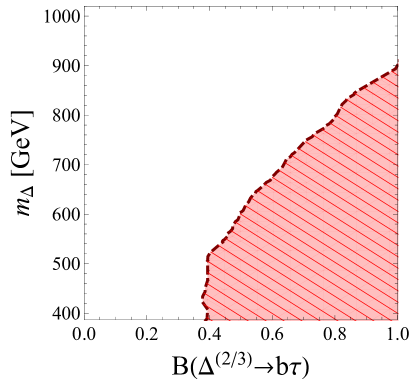
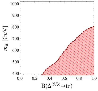
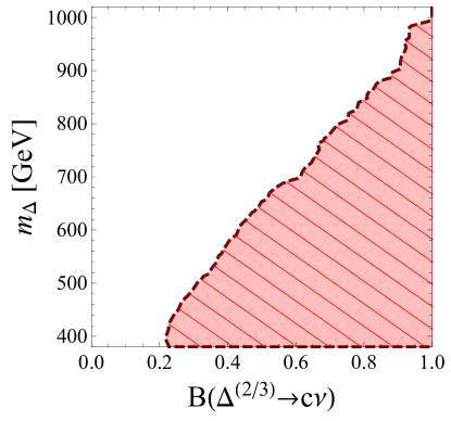
In any realistic scenario, the limits mentioned above have to be reinterpreted to account for values of the branching ratios smaller than one. The reinterpretation of these exclusion limits on $m_{\Delta}$ are shown in Fig. 4 as a function of ${\cal B}(\Delta^{(2/3)}\to b\tau)$ (upper left panel), ${\cal B}(\Delta^{(5/3)}\to t\tau)$ (upper right panel) and ${\cal B}(\Delta^{(2/3)}\to c\nu)$ (lower panel). In the scenario we are considering, cf. Eq. (4), the branching ratios read

$$\mathcal{B}(\Delta^{(2/3)}\to c\nu) =\dfrac{|g_{L}^{c\tau}|^{2}}{|g_{R}^{b\tau}|^{2}+|g_{L}^{c\tau}|^{2}}\,,\qquad\qquad\mathcal{B}(\Delta^{(2/3)}\to b\tau)=\dfrac{|g_{R}^{b\tau}|^{2}}{|g_{R}^{b\tau}|^{2}+|g_{L}^{c\tau}|^{2}}\,,$$ (20)

and

$$\mathcal{B}(\Delta^{(5/3)}\to t\tau) =\dfrac{|g_{R}^{b\tau}|^{2}\left(1-\dfrac{m_{t}^{2}}{m_{\Delta}^{2}}\right)^{2}}{|g_{R}^{b\tau}|^{2}\left(1-\dfrac{m_{t}^{2}}{m_{\Delta}^{2}}\right)^{2}+|g_{L}^{c\tau}|^{2}}\,,$$ (21)

where, for simplicity, we assumed $|V_{tb}|\approx 1$ and neglected the light fermion masses ($m_{c}$, $m_{b}$ and $m_{\tau}$). From the above formulas we conclude that scenarios with $m_{\Delta}\lesssim 1$ TeV can comply with the limits of Fig. 4 if the branching ratios are diluted by a large coupling to the charm quark. In other words, the ratio $|g_{R}^{b\tau}|/|g_{L}^{c\tau}|$ should be of $\mathcal{O}(1)$, which also agrees with the constraints on $g_{R}^{b\tau}$ derived from $Z\to\tau^{+}\tau^{-}$, cf. Eq. (13). We checked that $m_{\Delta}$ can be as low as $\approx 650$ GeV for some combinations of Yukawa couplings.

In Fig. 5, we confront the allowed region by $R_{D}$ with the indirect and direct constraints discussed above by assuming $g_{R}^{b\tau}$ to be purely imaginary, as discussed in Sec. 2.1. For instance, we see in these plots that both $|g_{R}^{b\tau}|$ and $g_{L}^{c\tau}$ are bounded from above by the $Z$-pole observables. Furthermore, the couplings needed to explain $R_{D}$ for $m_{\Delta}\lesssim 1~{}\mathrm{TeV}$ are not very large, mostly due to the CKM enhancement in Eq. (6), and they can therefore be perfectly consistent with phenomenological constraints discussed in this Section.

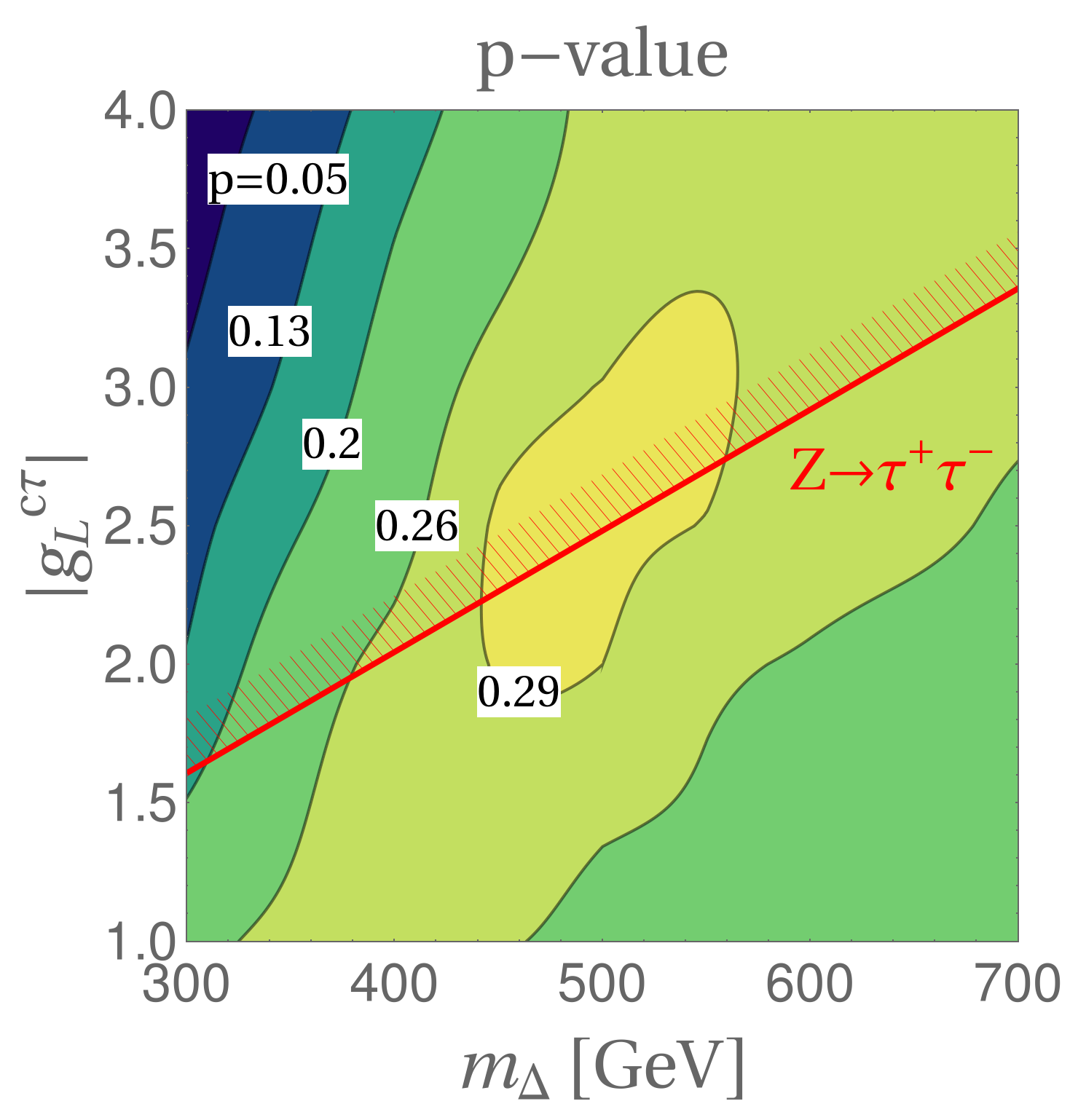
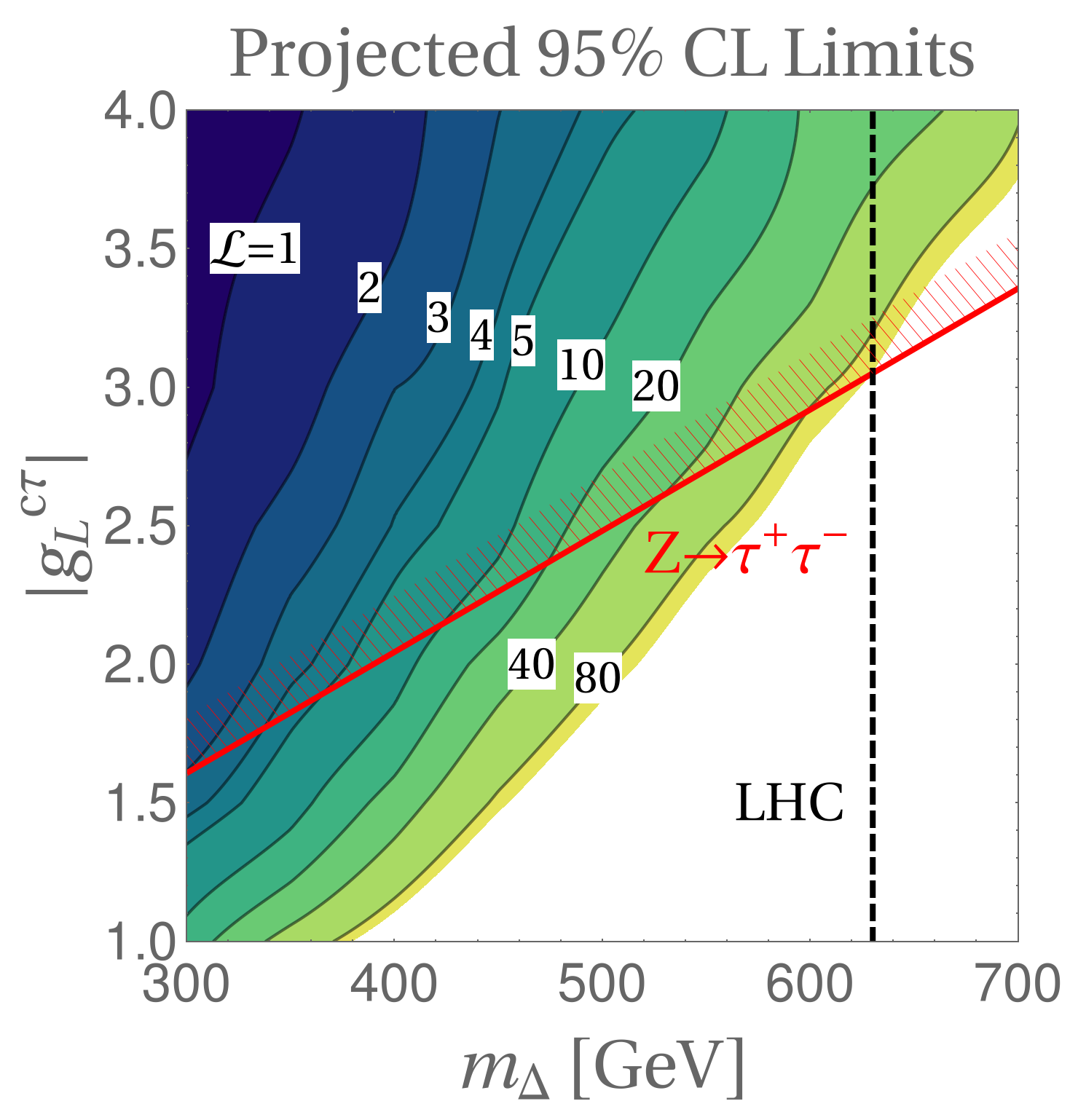
In what follows, we will discuss the IceCube phenomenology of the LQ scenario considered in this paper. In practice, we will focus on the analysis of the parameter space defined by $m_{\Delta}$ and $g_{L}^{c\tau}$ since they are the relevant parameters to determine IceCube signals. In this plane the region allowed by the $Z$-pole observables is approximately limited by a straight line, such that the allowed values are $g_{L}^{c\tau}\lesssim 1.6+1.3(m_{\Delta}/300\,\text{GeV}-1)$, which is also illustrated in this paper in Figs. 12 and 14.

Figure 5: The allowed region on the plane $g_{L}^{c\tau}\times|g_{R}^{b\tau}|$ by current experimental constraints is shown in yellow for $m_{\Delta}\in\{0.65,~{}0.8,~{}0.9\}$ TeV. We assume $g_{R}^{b\tau}$ to be a purely imaginary coupling, as described in the text. The separate allowed regions both from the direct searches at the LHC, the $Z$-pole observables and $R_{D}$ are shown from lighter to darker blue, respectively. Thus, the yellow region is given by their intersection. See text for details.

3 High Energy Neutrino Events in IceCube

The cubic kilometer IceCube Neutrino Observatory in the South Pole observed between 2010 and 2012 the first evidence of a diffuse flux of astrophysical neutrinos above 100 TeV Aartsen:2013jdh , which was further confirmed in the updated analyses Aartsen:2014gkd ; Aartsen:2015zva ; Aartsen:2017mau . In this paper we consider the 6-year sample Aartsen:2017mau which contains 80 High Energy Starting Events (HESE). In particular, we focus on the 28 events with deposited energies above 100 TeV, which are divided in 23 showers and 5 tracks. This flux, of yet unknown astrophysical origin, seems to be isotropic and consistent with a single power law behavior followed by neutrinos and antineutrinos of all flavors Aartsen:2015ivb . In other words, the neutrino energy spectrum can be parameterized by a spectral index, $\gamma$, and a normalization constant $\rm C_{0}$ as

$$\frac{d\Phi_{\nu}}{dE_{\nu}}=\frac{\rm C_{0}}{10^{8}}\left(\frac{E_{\nu}}{100\;\rm TeV}\right)^{2-\gamma}\frac{1}{E_{\nu}^{2}}\quad{\rm[GeV^{-1}\;cm^{-2}\;str^{-1}\;s^{-1}]}\,,$$ (22)

so that at the Earth the flavor fluxes are given by

$$\frac{d\Phi_{\alpha}}{dE_{\nu}}=f^{\oplus}_{\alpha}\;\frac{d\Phi_{\nu}}{dE_{\nu}}\,,$$ (23)

where $f^{\oplus}_{\alpha}$, $\alpha=\{\nu_{e},\nu_{\mu},\nu_{\tau},\bar{\nu}_{e},\bar{\nu}_{\mu},\bar{\nu}_{\tau}\}$, are the normalized neutrino and antineutrino flavor fractions at the Earth.

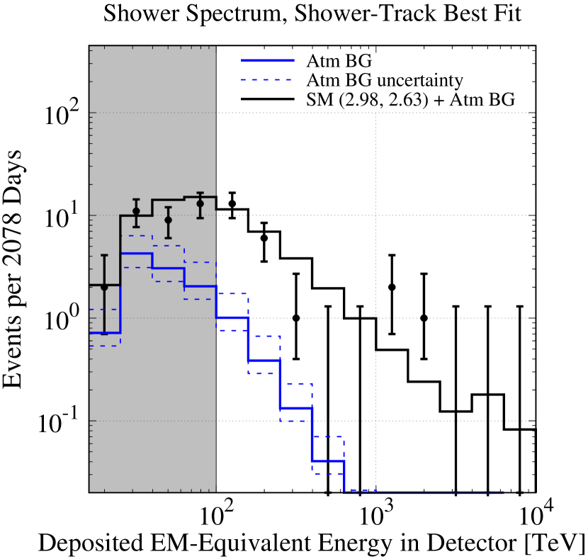
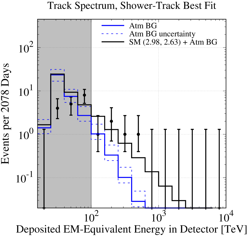
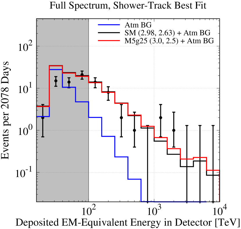
Assuming the flavor composition to be the standard one expected from neutrino oscillations, i.e., $(f^{\oplus}_{\nu_{e}}:f^{\oplus}_{\nu_{\mu}}:f^{\oplus}_{\nu_{\tau}})=(f^{\oplus}_{\bar{\nu}_{e}}:f^{\oplus}_{\bar{\nu}_{\mu}}:f^{\oplus}_{\bar{\nu}_{\tau}})=(1:1:1)$, IceCube best fit of 6-year sample yields $\gamma=2.92^{+0.33}_{-0.29}$ and ${\rm C_{0}}=2.46\pm 0.8$ GeV cm^-2 str^-1 s^-1 Aartsen:2017mau . To test our fitting procedure we used the publicly available IceCube data, fit them to the SM and obtained 

$$\gamma~{}=~{}2.98^{+0.42}_{-0.38}\,,\qquad\qquad{\rm C_{0}}=2.63^{+1.87}_{-1.23}~{}\mathrm{GeV}\,\mathrm{cm}^{-2}\,\mathrm{str}^{-1}\,\mathrm{s}^{-1}$$ (24)

with a p-value of 0.25, in full agreement with the above-mentioned IceCube results Aartsen:2017mau . The best fit curves for shower and track spectra are shown in Fig. 6.  For simplicity, in the fit we have used a fixed atmospheric background spectrum which is derived from the central values for the total amount of atmospheric neutrinos estimated in Aartsen:2017mau , which are $N_{\mu}=25.2\pm 7.3$ and $N_{\text{atm}}=15.6^{+11.4}_{-03.9}$. To reduce the effects of uncertainties we focus on the energy range [100 TeV, 10 PeV], in which the background contribution is sub-leading. Indeed, the computation of the best fit considering the minimum (maximum) expectations for the atmospheric background yields $\gamma=3.0\,(2.9)$ and $C_{0}=2.7\,(2.4)$ with a p-value of 0.24 (0.23), which lies perfectly inside the allowed 1$\sigma$ region. We will apply the same strategy to analyze LQ scenarios. Before passing onto that discussion we examine some aspects of the simulation of IceCube events, with special attention to the new contributions introduced by LQ interactions.

Figure 6: Standard Model best fit of the IceCube 6-year dataset in the energy range [100 TeV, 10 PeV], which gives the values $\gamma=2.98$ and ${\rm C_{0}}=2.63$ GeV cm^-2 str^-1 s^-1 for the neutrino flux parameters. The atmospheric background is computed from the estimated central values given in Ref. Aartsen:2017mau , from which we obtained $N_{\mu}=25.2$ and $N_{\text{atm}}=15.6$. The points in the grey region are not included in the fit, as discussed in the text.

3.1 Calculation of the Event Rate in IceCube

Icecube detects individual neutrino events through the Cherenkov radiation emitted by charged secondary particles produced in the neutrino interaction with the Antarctic ice. These events are characterized by the electromagnetic (EM) equivalent of the total deposited energy in the detector ($E_{\rm dep}$) and their topology (track or shower). Within the SM, track events can only arise when $\nu_{\mu}$ or $\bar{\nu}_{\mu}$ interact with nucleons via charged current (CC) interactions, producing a energetic muon or antimuon. On the other hand, shower events can be induced by CC interactions of $\overset{\textbf{(---)}}{\nu_{e}}$ and $\overset{\textbf{(---)}}{\nu_{\tau}}$ or by neutral current (NC) interactions of all (anti-)neutrino flavors with nucleons.

To calculate the number of shower (sh) or track (tr) events produced by SM interactions in an interval of reconstructed energy [$E_{\rm dep}$,$E_{\rm dep}+dE_{\rm dep}$], we first calculate the individual contributions to the event rate via the expression,

$$\frac{dN^{\rm c,h,X}_{\alpha}}{dE_{\rm dep}}=TN_{A}\int_{0}^{\infty}dE_{\nu}\,{\cal A}^{\rm h}_{\alpha}(E_{\nu})\frac{d\Phi_{\alpha}}{dE_{\nu}}\int_{0}^{1}dy\,{\cal M}_{\rm eff}(E_{\rm t})\,R(E_{\rm t},E_{\rm dep},\sigma_{E_{\rm t}})\,\frac{d\sigma^{\rm X}_{\alpha}}{dy}\,,$$ (25)

where $\rm c=sh,tr$ indicates the type of topology, $\rm h={S,N}$ the events entering the detector from the south (S) or north (N) hemisphere, and $\rm X=\mathit{NC},\mathit{CC},e$-scattering stands for the different type of processes we consider. Here, $T$ is the exposure time in seconds, $N_{A}~{}=~{}6.022~{}\times~{}10^{23}$ g^-1 is the Avogadro’s number times the number of moles per each gram of protons/neutrons, and ${\cal A}^{\rm h}_{\alpha}$ accounts for the effect of Earth’s attenuation, c.f. Eq.(3.3). The effective mass of the detector in grams is denoted by ${\cal M}_{\rm eff}(E_{\rm t})$, which corresponds to the mass of the target material convoluted with the efficiency of converting an event with true deposited energy $E_{\rm t}$ into the observed signal. The resolution function, $R(E_{\rm t},E_{\rm dep},\sigma_{E_{\rm t}})$, is taken to be a Gaussian distribution with mean equal to the true deposited energy $E_{\rm t}$ and standard deviation $\sigma_{E_{\rm t}}$, both clearly dependent on the particular process taking place. Finally, $d\sigma^{\rm X}_{\alpha}/dy$ is the differential cross section for process $\rm X$ in the inelasticity interval $[y,y+dy]$. Our calculations were performed in the same way as described in Refs. Nunokawa:2016pop and Palomares-Ruiz:2015mka , and we refer to these papers for further details.

3.2 Leptoquark Contribution to the Event Rate

In our model, only the coupling $g_{L}^{c\tau}$ affects the neutrino-nucleon production cross section at IceCube, c.f. Eq. (3). The other coupling, $g_{R}^{b\tau}$, only contributes to the total decay width of the LQ bosons. In this case, since the new interactions only involves quarks, neutrinos and $\tau$-leptons, this scenario will only produce nonstandard shower-like events in IceCube. The event rate with $\nu_{\tau}$ in Eq. (25) will then receive the New Physics contribution

$$\frac{dN^{\rm sh,h,\Delta}_{\nu_{\tau}}}{dE_{\rm dep}}=TN_{A}\int_{0}^{\infty}dE_{\nu}\,{\cal A}^{\rm h}_{\nu_{\tau}}(E_{\nu})\frac{d\Phi_{\nu_{\tau}}}{dE_{\nu}}\int_{y_{\rm min}}^{y_{\rm max}}dy\,{\cal M}_{\rm eff}(E_{t})\,R(E_{t},E_{\rm dep},\sigma_{E_{t}})\,\frac{d\sigma^{\rm\Delta}_{\nu_{\tau}}}{dy},\,$$ (26)

where the differential cross-section expressions $d\sigma_{\nu_{\tau}}^{\Delta}/dy$ can be found in Appendix A, with $y$ being the inelasticiy variable. The same expression applies mutatis mutandis to the $\bar{\nu}_{\tau}$ event rate.

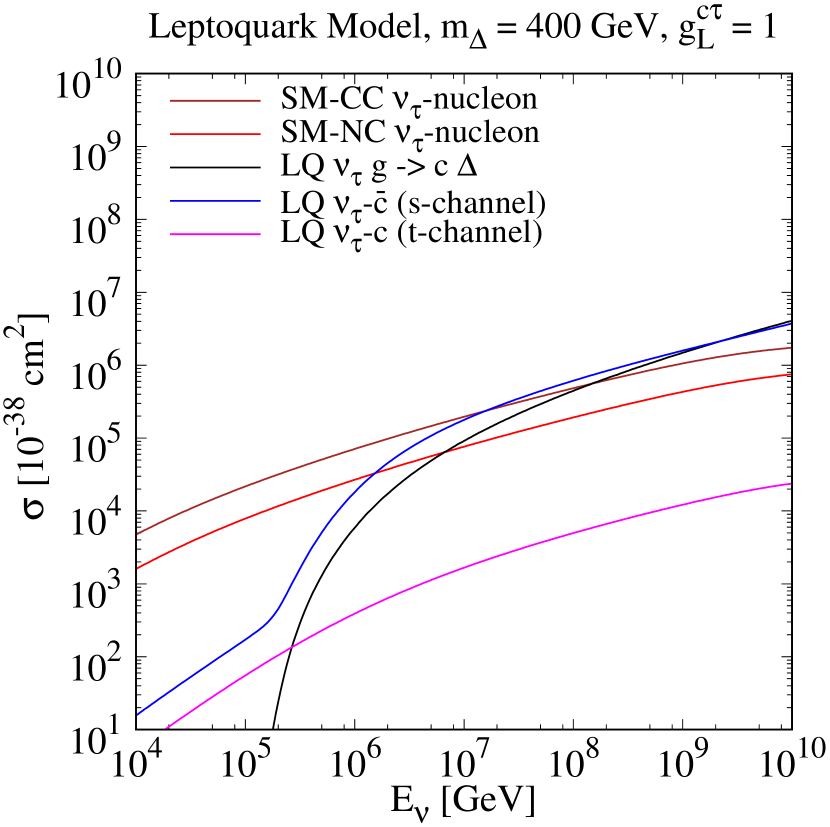
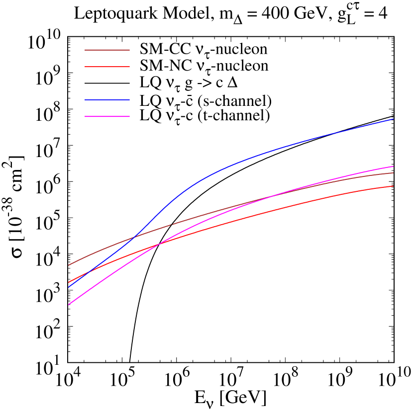
In previous LQ studies Anchordoqui:2006wc ; Barger:2013pla ; Dutta:2015dka ; Dey:2017ede ; Mileo:2016zeo ; Dey:2015eaa ; Chauhan:2017ndd , only the parton level processes $\nu_{\ell}+\overset{\textbf{(---)}}{q}\to\nu_{\ell}+\overset{\textbf{(---)}}{q}$ were considered in the cross-section, c.f. Fig. 7. In addition to the interaction with quarks, high-energy neutrinos can also interact with gluons via the transition $\nu_{\ell}+g\to q_{u}+\Delta$, with the LQ decaying inside the detector, as shown in Fig. 8. This contribution to the cross-section can be of the same order of the $\nu_{\ell}+q$ contribution when dealing with heavy quarks, $q\in\{c,b\}$, and thus cannot be neglected, as we illustrate in Fig. 9. This can be understood from the suppression of the $s$- and $t$-channel interactions with heavy quarks by the small values of the parton distribution functions (PDFs). Furthermore, the gluon PDF shows a fast growth when the Bjorken scale variable $x$ approaches zero, giving a non-negligible contribution to heavy quark cross-sections.

Figure 7: Feynman diagrams contributing to $\nu_{\ell}+q_{u}\to{\nu}_{\ell^{\prime}}+q_{u^{\prime}}$ and $\nu_{\ell}+\bar{q}_{u}\to{\nu}_{\ell^{\prime}}+\bar{q}_{u^{\prime}}$ via a LQ exchange. Here $\nu_{\ell},\nu_{\ell^{\prime}}$ are generic neutrino flavors and $q_{u},q_{u^{\prime}}$ are generic up-type quarks.

Figure 8: Feynman diagrams contributing to the process $g+\nu_{\ell}\to q_{u}+\Delta$, where the LQ particle decays into $\bar{q_{u}}+\nu_{\ell^{\prime}}$.

Figure 9: $\nu_{\tau}$-nucleon cross sections: CC contribution in the SM, NC contribution in the SM, $\nu_{\tau}$-gluon contribution, $\nu_{\tau}$-c-quark s-channel contribution, $\nu_{\tau}$-c-quark t-channel contribution. For the LQ cross sections $m_{\Delta}=400$ GeV and $g_{L}^{c\tau}=1$ (left) and $g_{L}^{c\tau}=4$ (right).

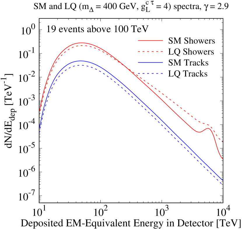
To estimate the impact of LQ interactions to the IceCube data we compare in Fig. 10 the distribution of shower and track events generated by the SM and two representative LQ scenarios. These results were obtained under the restriction of a fixed total number of events. We see that the nonstandard effects appear only at high neutrino energies ($E_{\nu}\gtrsim 500$ TeV), anticipating a modest sensitivity to LQs with current IceCube data. This instigates us to investigate the situation with maximal future sensitivity of IceCube and IceCube-Gen2 Aartsen:2015dkp which we postpone to Sec. 4.

Figure 10: Comparison between the distribution of shower and track events for the SM and two representative LQ scenarios: $m_{\Delta}=400$ GeV and $g_{L}^{c\tau}=1$ (left panel) and $m_{\Delta}=400$ GeV and $g_{L}^{c\tau}=4$ (right panel). Notice that the LQ shower (and track) distributions include both the contribution of the SM as well as of the LQ interactions.

3.3 Attenuation and Regeneration Effects

The neutrinos that arrive in IceCube from the south hemisphere do not suffer Earth effects, having then an attenuation factor of ${\cal A}^{\rm S}_{\alpha}(E_{\nu})=\frac{1}{2}$ for an isotropic flux in Eq. (25). The neutrinos entering from the north hemisphere have to go through the Earth before reaching the IceCube detector with the attenuation factor of the resulting flux given by

$${\cal A}^{\rm N}_{\alpha}(E_{\nu})=\frac{1}{2}\int_{0}^{1}{\cal A}_{\alpha}(E_{\nu},\theta)\;\;d\cos\theta\,,$$ (27)

where $\theta$ is the nadir angle, and

$${\cal A}_{\alpha}(E_{\nu},\theta)\equiv\frac{{\cal F}_{\alpha}(E_{\nu},X(\theta))}{{\cal F}_{\alpha}(E_{\nu},0)}\,,$$ (28)

is simply a fraction of the initial flux after propagating though a column depth $X(\theta)$,

$$X(\theta)=\int_{0}^{L(\theta)}\rho(s)\,ds\,,$$ (29)

where $\rho(s)$ is the matter density at the point $s$, $L(\theta)=2R_{\oplus}\cos\theta$, and $R_{\oplus}$ is the Earth’s radius. In the above formulas, the function ${\cal F}_{\alpha}$ is defined by

$${\cal F}_{\alpha}(E,X(\theta))\equiv\frac{\partial\Phi_{\alpha}}{\partial E}(E,X(\theta))\,.$$ (30)

To calculate ${\cal A}^{\rm N}_{\alpha}(E_{\nu})$ we need to solve the coupled integro-differential transport equations given in Appendix B which include absorption and regeneration effects via particle decays. We have followed the prescription described in Ref. Rakshit:2006yi to numerically solve these equations. Furthermore, we assumed that the absorption of $\tau$ and $\Delta^{(2/3)}$ is only given by their decays into lighter particles, neglecting the subdominant scattering contributions.

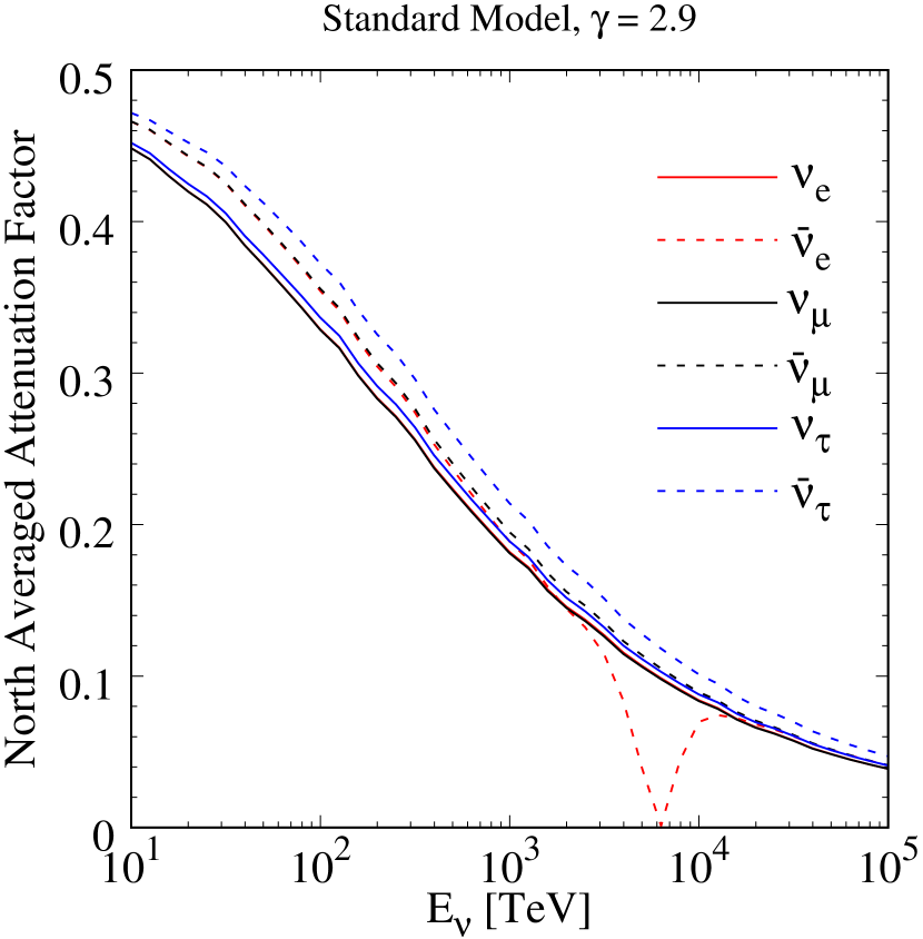
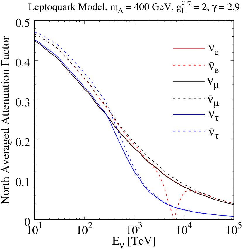
The average attenuation factor ${\cal A}^{\rm N}_{\alpha}(E_{\nu})$ for each (anti-)neutrino flavor is shown in Fig. 11 for the SM (left panel), and for a LQ scenario with $m_{\Delta}=400$ GeV and $g_{L}^{c\tau}=2$ (righ panel). As expected, the attenuation factors ${\cal A}^{\rm N}_{\nu_{\tau}}$ (${\cal A}^{\rm N}_{\bar{\nu}_{\tau}}$) are highly affected by LQ interactions for $E_{\nu}\gtrsim 500$ TeV. Note, however, that since the incoming flux falls rapidly with $E_{\nu}$, this effect turns out to be smaller than suggested by Fig. 11. Furthermore, we included the regeneration effects in our simulation which can lower the attenuation factors by at most 10%.

Figure 11: Average attenuation factor ${\cal A}^{\rm N}_{\alpha}(E_{\nu})$ for each (anti-)neutrino flavor for the SM (left panel) and for a LQ model with $m_{\Delta}=400$ GeV and $g_{L}^{c\tau}=2$ (right panel). These results has been obtained by fixing $\gamma=2.9$, but they only show a mild dependence on this parameter.

4 Statistical Data Analysis at IceCube, Present and Future

As stated in previous Sections, we use the 6-year HESE sample in the energy range [100 TeV, 10 PeV] Aartsen:2017mau . To quantify the goodness-of-fit of each model we follow the maximum likelihood method described in Ref. Aartsen:2015knd . The test statistic is defined by

$$-2\ln L(H)/L_{\text{sat}}=-2\sum_{i}^{N_{\text{bins}}}\ln(e^{o_{i}-n_{i}}(n_{i}/o_{i})^{o_{i}})\,,$$ (31)

where $L(H)$ is the likelihood of the tested hypothesis $H$ (product of Poisson probabilities), and $L_{\text{sat}}$ is the likelihood of the model that predicts the exact observed outcome, $\mbox{i.e.}\,\,n_{i}\equiv o_{i}$. Moreover, the values of $o_{i}$ and $n_{i}$ correspond to the observed and predicted number of events in the bin $i$, respectively. We divide the events sample in the neutrino energy range [100 TeV, 10 PeV] in $10$ logarithmic energy bins for tracks and as many for showers. The total number of bins, $N_{\text{bins}}=20$, is comparable to the 28 events detected above 100 TeV. We consider a track to shower misidentification factor (missID) of 20%, which is reasonable considering that IceCube has measured it to be approximately 30% for low energy tracks Aartsen:2015ivb and since it is expected to decrease with energy. Nevertheless, we have verified that the final results are unaffected by using a 10% or a 30% missID factor, similarly to what has been obtained in Ref. Dey:2017ede .

We reiterate that in our statistical analysis we consider 5 parameters:

$$\gamma,\,C_{0},\,m_{\Delta},\,g_{L}^{c\tau},\,g_{R}^{b\tau},$$ (32)

which we vary as $m_{\Delta}\in[300\,\text{GeV},700\,\text{GeV}]$, $|g_{L}^{c\tau}|\in[1,4]$, and we set $g_{R}^{b\tau}\approx 0$ since it does not directly contribute to the cross-sections relevant to this study.

4.1 Current Data Analysis

To evaluate the quality of the fit of a hypothesis H with respect to current data, we compute the minimum of the test statistic (31) and its corresponding p-value, obtained by simulating pseudo-data with the best fit values of $\gamma$ and $C_{0}$. As already mentioned in the text, we find that the SM best fit point yields $\gamma=2.98$ and ${\rm C_{0}}=2.63$ GeV cm^-2 str^-1 s^-1 with a test statistic value of 17.05, and a p-value of 0.25. This indicates that the SM compatibility with the current data is quite acceptable.

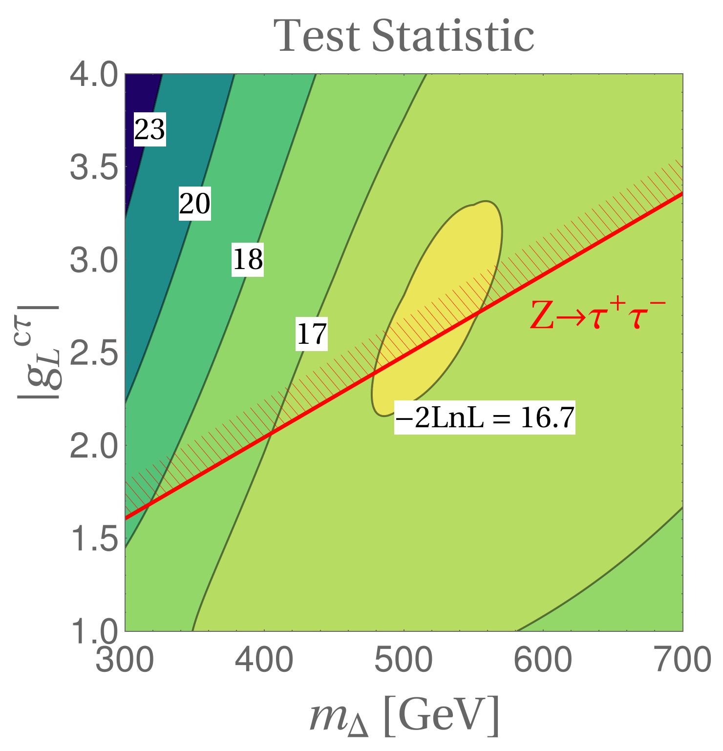
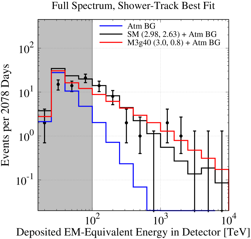
The results obtained in the LQ scenario are shown in Fig. 12 for different values of LQ mass $m_{\Delta}$ and coupling $|g_{L}^{c\tau}|$. We find that the best fit point is given by $(m_{\Delta},\,|g_{L}^{c\tau}|)=(500\,\text{GeV},\,2.5)$ with a minimum test statistic of 16.7, and therefore the event distribution of the SM and the best LQ model are indistinguishable from the IceCube data, also shown in left panel of Fig. 13. From the right panel of Fig. 13 we learn that only LQ models with very large $g_{L}^{c\tau}\approx 3.5$ and small masses $m_{\Delta}\approx 300$ GeV can be excluded by current IceCube data to $95\%$ CL ($p\leq 0.05$). These parameters, however, are already excluded by the limits arising from the $Z$-pole observables, as discussed in Sec. 2.

Figure 12: Summary of the best fit analysis of LQ models characterized by the values of $m_{\Delta}$ and $|g_{c\tau}|$. These results are based on the minimization of the test statistic defined in Eq. (31) with respect to $\gamma$ and $C_{0}$ using the IceCube 6-year data sample. In the left panel we show contour lines for the values of the test statistic, while in the right panel we also plot contour lines but considering the obtained p-value. We show in both figures the exclusion coming from the $Z$-pole observables discussed in Sec. 2.2.

Figure 13: Comparison between the SM and LQ best fit curves to the IceCube 6-year dataset. In the left panel we show the best fit curve for $(m_{\Delta},\,|g_{L}^{c\tau}|)=(500\,\text{GeV},\,2.5)$, which is one representative case of scenarios with $-2\ln L=16.7$. In the right panel, we show the best fit curve for $(m_{\Delta},\,|g_{L}^{c\tau}|)=(300\,\text{GeV},\,4)$, which has a p-value around 0.05 and therefore it is in tension with current data. In the plot legend we quote within parentheses the best fit values of $\gamma$ and $C_{0}$ for each model.

4.2 Future IceCube(-Gen2) Projections

To investigate the projected sensitivity of IceCube to our LQ scenario, we compute the projected exclusion regions in the plane $(m_{\Delta},\,|g_{L}^{c\tau}|)$ by assuming the SM is the null hypothesis. We considered the test statistic defined by the likelihood ratio between the LQ and the SM hypotheses, given by $q=-2\log L(\text{LQ})/L(\text{SM})$ with $L(\text{LQ})$ and $L(\text{SM})$ defined analogously to Eq. (31). The value of $q$ is obtained after the minimization of each hypothesis with respect to $(\gamma,C_{0})$ by using projected data, which is generated from Monte Carlo simulations of the SM best fit to current data. More specifically, we evaluate the luminosity $\mathcal{L}$, at which the projected data is simulated, by using multiples of current 6-year exposure. To establish a criteria for exclusion we consider the p-value associated to each tested value of $q$. We simply assume that $q$ follows a $\chi^{2}$-distribution with $k$ degrees of freedom, where $k$ is the difference in the number of parameters between the LQ and SM hypotheses, which in our case is $k=2$. Thus, for a given value of $q$, the p-value is given by $p=\exp(-q/2)$.

In Fig. 14 we plot our results as the projected 95% CL exclusion regions in the $(m_{\Delta},\,|g_{L}^{c\tau}|)$ plane, along with the limits arising from the $Z$-pole observables, as well as the region eliminated by the reinterpretation of LHC searches for pair-produced LQs decaying into $b\tau$ Khachatryan:2016jqo ; CMS:2016hsa , $c\nu$ CMS:2018bhq and $t\tau$ Khachatryan:2015bsa ; Sirunyan:2018nkj , c.f. discussion in Section 2. We see that the parameter region accessible to IceCube increases at a modest pace with the luminosity $\mathcal{L}$, reaching the corners ($m_{\Delta}=300$, $|g_{L}^{c\tau}|=1$) and ($m_{\Delta}=600$, $|g_{L}^{c\tau}|=4$) only with about $20$ and $40$ times more events than the current data. An exposure equivalent to $10$ ($40$) times the current one might be within reach of IceCube-Gen2 Aartsen:2015dkp after about $5$ ($20$) years of data taking. From that plot we also see that the region of parameters accessible to IceCube(-Gen2) is already disfavored by a combination of constraints arising from the direct (LHC) and indirect searches (flavor physics and LEP).

Figure 14: Estimation of the 95% CL exclusion regions in the parameter space ($m_{\Delta}$, $|g_{L}^{c\tau}|$) considering several projections of IceCube data at exposures measured in units of the current 6-year data sample. We also show the constraints on large LQ couplings derived from the $Z$-pole observables (red line) and the lower limits on the LQ mass stemming from the reinterpretation of LHC limits on pair-produced LQs (dashed line), see Sec. 2.2 for details.

5 Conclusions

Several authors have inquired about the potential of IceCube detector in the South Pole to search for LQs Anchordoqui:2006wc ; Barger:2013pla ; Dutta:2015dka ; Mileo:2016zeo ; Dey:2015eaa ; Chauhan:2017ndd ; Dey:2017ede . In most of these works LQs couple to the first generation of quarks. On the one hand this allows LQ production to profit from the valence quark contribution to the neutrino-nucleon cross section. On the other hand limits from direct searches, atomic parity violation and flavor physics are at odds with these possibilities.

Here, instead, we focus on LQs that couple to heavy quark flavors, a scenario that recently became of particular interest in connection with $B$-meson semileptonic decays. The hope that IceCube could contribute to the search of this type of LQ models springs from a few considerations. First, these models cannot be dismissed by current direct or indirect detection searches. Second, their production cross section has been underestimated in the literature as the neutrino-gluon contribution has been neglected up to now. Third, attenuation effects when crossing the Earth are modified by the new LQ interactions which was not considered previously. Finally, the proposal of IceCube-Gen2 Aartsen:2015dkp allows for exploring a much higher statistics of HESE than at the present time.

In this paper we focused on a simple LQ scenario that can explain $R_{D^{(\ast)}}^{\mathrm{exp}}>R_{D^{(\ast)}}^{\mathrm{SM}}$ and involves only three new parameters: the LQ mass ($m_{\Delta}$) and two couplings ($g_{L}^{c\tau}$ and $g_{R}^{b\tau}$). Parameter space is constrained in such a way as to solve $R_{D^{(\ast)}}$ and satisfy experimental constraints coming from the $Z$-decay modes. With parameters constrained in this way we estimate the present (future) sensitivity of IceCube (IceCube-Gen2) to this model. Our results are summarized in Fig. 14 from which we see that the parameter space accessible to IceCube/IceCube-Gen2 is already excluded by the direct searches (see Fig. 4) and the low-energy flavor physics observables. That conclusion is based on our current understanding of the HESE data and the value of the spectral index $\gamma$ in particular. If that value turns out to be lower, then also Fig. 14 would change because there would be more data corresponding to heavier LQs but with the mass still lower than about $650$ GeV, to comply with the results of the direct searches at LHC.

We should also stress that in our calculation we consistently used a democratic flavor distribution of the incoming flux, which is plausible and compatible with the current data. Other possibilities are, however, possible too which is one reason more why settling that issue is of major importance for searching the effects of physics beyond the SM Aartsen:2017mau .

Appendix A Leptoquark Contributions to the Neutrino-Nucleon Scattering Cross Section

For completeness we give here the expressions for the neutrino-nucleon scattering cross section at the parton level. The total differential cross section induced by LQs can be written as

$$\frac{d\sigma^{\Delta}_{\nu_{\tau}}}{dy}(y,E_{\nu}) = \int_{x_{\rm min}}^{1}dx\,g(x,\hat{s})\,\frac{\partial^{2}\sigma^{g\nu_{\tau}}}{\partial x\partial y}(E_{\nu},x,y)$$ (33)

$$+ \sum_{q}\int_{0}^{1}dx\,q(x,\hat{s})\,\frac{\partial^{2}\sigma^{q\nu_{\tau}}}{\partial x\partial y}(E_{\nu},x,y)\,,$$

for an incident neutrino $\nu_{\tau}$. Here $g(x,\hat{s})$ ($q(x,\hat{s})$) is the gluon (quark $q$) PDF of the nucleon. In our computaions, we considered the NNPDF2.3 PDF sets Ball:2012cx , which are implemented in LHAPDF6 Buckley:2014ana .

A.1 $\nu_{\ell}$-gluon contribution

We give here the expressions for the gluon-neutrino differential cross sections induced by LQs. The kinematics of these processes can be described by the following variables

$$y=\frac{E_{\nu}-E_{\Delta}}{E_{\nu}}\,,\quad\quad x=\frac{Q^{2}}{2m_{N}E_{\nu}\,y}\,,\quad\quad\hat{s}=2x\,m_{N}E_{\nu}\,,$$

with the inelasticity $y$ and the Bjorken variable $x$ defined in the intervals 

$$y\in\left[\frac{\hat{s}-m_{q}^{2}-m_{\Delta}^{2}-\lambda^{1/2}(\sqrt{\hat{s}},m_{\Delta},m_{q})}{2\hat{s}},\frac{\hat{s}-m_{q}^{2}-m_{\Delta}^{2}+\lambda^{1/2}(\sqrt{\hat{s}},m_{\Delta},m_{q})}{2\hat{s}}\right]\,,$$

and

$$x\in\left[\frac{(m_{q}+m_{\Delta})^{2}}{2m_{N}E_{\nu}},1\right]\,,$$

where $E_{\nu}$ and $E_{\Delta}$ are the (anti-)neutrino and LQ energies in the laboratory frame, $Q^{2}=-t$ is the invariant squared momentum transfered in the $t$-channel, $m_{q}$ is the mass of the quark in the process, $m_{\Delta}$ the LQ mass, and $m_{N}=(m_{p}+m_{n})/2$ is the average mass of the nucleon. We have used the fact that water is a isoscalar target, so that $N=Z$. We also define the function $\lambda(a,b,c)\equiv(a^{2}-(b-c)^{2})(a^{2}-(b+c)^{2})$.

The two diagrams that contribute to the amplitudes that enter these cross sections can be seen in Fig. 8. The cross section for $\nu_{\ell}\,g\to q_{u}\,\Delta^{(-2/3)}$ is given by 

$$\frac{\partial^{2}\sigma^{g\nu_{\ell}}}{\partial x\partial y}=(2m_{p}E_{\nu}x)\frac{\alpha_{s}|g_{L}^{q_{u}\ell}|^{2}}{8\hat{s}} \Bigg{\{}\frac{\hat{s}Q^{2}+m_{q}^{2}[2(m^{2}_{\Delta}+Q^{2})+\hat{s}]}{(m_{q}^{2}+Q^{2})^{2}}$$ (34)

$$+\frac{(Q^{2}+m^{2}_{\Delta}-\hat{s})(2m_{\Delta}^{2}+Q^{2}-\hat{s}+m_{q}^{2})}{(m_{q}^{2}+Q^{2}-\hat{s})^{2}}$$

$$+\frac{(\hat{s}-Q^{2}-m^{2}_{\Delta})(2m_{\Delta}^{2}+Q^{2})+m_{q}^{2}[\hat{s}-3(Q^{2}+m_{\Delta}^{2})]}{(m_{q}^{2}+Q^{2})(m_{q}^{2}+Q^{2}-\hat{s})}\Bigg{\}}\,,$$

where $N_{c}$ is the number of colors $q_{u}$ and $\ell$ are a generic up-type quark and lepton, and $\alpha_{s}=\alpha_{s}(\hat{s})$ is the strong coupling constant at the relevant scale of the process.

A.2 $\nu_{\ell}$-quark contribution

The LQ state contributes to the neutrino-quark cross-section via an exchange of a LQ in the $t$-channel as depicted in Fig. 7. The SM cross-section ammended with the LQ contribution reads

$$\dfrac{\partial^{2}\sigma^{\nu_{\ell}{q_{u}}\to\nu_{\ell^{\prime}}{q}_{u^{\prime}}}}{\partial x\partial y} =\dfrac{2m_{p}E_{\nu}x}{32\pi\hat{s}^{2}}\Bigg{\{}\dfrac{\hat{u}^{2}\,|g_{L}^{q_{u}\ell^{\prime}}|^{2}|g_{L}^{q_{u^{\prime}}\ell}|^{2}}{(\hat{u}-m_{\Delta}^{2})^{2}}$$ (35)

$$+\delta_{\ell\ell^{\prime}}\delta_{\hat{u}u^{\prime}}\Bigg{[}|g_{L}^{u\ell}|^{2}\dfrac{16\sqrt{2}G_{f}m_{Z}^{2}u^{2}(g_{A}^{u}-g_{V}^{u})}{(\hat{u}-m_{\Delta}^{2})(\hat{t}-m_{Z}^{2})}$$

$$+\dfrac{8G_{F}^{2}m_{Z}^{4}\left[(\hat{s}^{2}+\hat{u}^{2})\left(\left(g_{A}^{u}\right)^{2}+\left(g_{V}^{u}\right)^{2}\right)+2g_{A}^{u}g_{V}^{u}(\hat{s}^{2}-\hat{u}^{2})\right]}{(\hat{t}-m_{Z}^{2})^{2}}\Bigg{]}\Bigg{\}}\,,$$

where $q_{u},q_{u^{\prime}}$ are generic up-type quarks and $\ell,\ell^{\prime}$ are generic leptons. We define the weak couplings $g_{V}^{u}=T_{u}^{3}-2Q_{u}\sin^{2}\theta_{W}=1/2-4/3\sin^{2}\theta_{W}$ and $g_{A}^{u}=T_{u}^{3}=1/2$. The Mandelstam variables in our setup are taken to be

$$\hat{s} =(p_{\nu_{\ell}}+p_{q_{u}})^{2}\,,\qquad\hat{t}=(p_{\nu_{\ell}}-p_{\nu_{\ell^{\prime}}})^{2}\,\quad\text{and}\quad\hat{u}=(p_{\nu_{\ell}}-p_{q_{u^{\prime}}})^{2}.$$ (36)

Similarly, the $\nu\bar{q}$ cross-section receives a $s$-channel contribution from the LQ state, as shown in Fig. 7. The corresponding expression is given by

$$\dfrac{\partial^{2}\sigma^{\nu_{\ell}\bar{q}_{u}\to\nu_{\ell^{\prime}}\bar{q}_{u^{\prime}}}}{\partial x\partial y} =\dfrac{2m_{p}E_{\nu}x}{32\pi\hat{s}^{2}}\Bigg{\{}\dfrac{\hat{u}^{2}\,|g_{L}^{q_{u}\ell^{\prime}}|^{2}|g_{L}^{q_{u^{\prime}}\ell}|^{2}}{(\hat{s}-m_{\Delta}^{2})^{2}+m_{\Delta}^{2}\Gamma_{\Delta}^{2}}$$ (37)

$$+\delta_{\ell\ell^{\prime}}\delta_{uu^{\prime}}\Bigg{[}|g_{L}^{u\ell}|^{2}\dfrac{16\sqrt{2}G_{f}m_{Z}^{2}\hat{u}^{2}(g_{A}^{u}-g_{V}^{u})(\hat{s}-m_{\Delta}^{2})}{((\hat{s}-m_{\Delta}^{2})^{2}+m_{\Delta}^{2}\Gamma_{\Delta}^{2})(\hat{t}-m_{Z}^{2})}$$

$$+\dfrac{8G_{F}^{2}m_{Z}^{4}\left[(\hat{s}^{2}+\hat{u}^{2})\left(\left(g_{A}^{u}\right)^{2}+\left(g_{V}^{u}\right)^{2}\right)+2g_{A}^{u}g_{V}^{u}(\hat{s}^{2}-\hat{u}^{2})\right]}{(\hat{t}-m_{Z}^{2})^{2}}\Bigg{]}\Bigg{\}}\,.$$

where $\Gamma_{\Delta}$ is the total LQ decay width.

Appendix B Transport Equations Including the Leptoquark Constribution

The set of transport equations that have to be solved in order to compute the attenuation factor for the neutrino flux is the following

$$\frac{\partial{\cal F}_{\nu_{\ell}}}{\partial X} = -N_{A}[\sigma_{\nu_{\ell}N}^{\rm CC}(E)+\sigma_{\nu_{\ell}N}^{\rm NC}(E)+\sigma_{\nu_{\ell}}^{\Delta}(E)]{\cal F}_{\nu_{\ell}}(E,X)$$ (38)

$$+ \frac{1}{c\rho(X)}\int_{0}^{1}\frac{1}{1-y}\left[\frac{d\Gamma_{\tau\to\nu_{\ell}X^{\prime}}}{dy}(E_{y},y){\cal F}_{\tau}(E_{y},X)+\frac{d\Gamma_{\Delta\to\nu_{\ell}X^{\prime}}}{dy}(E_{y},y){\cal F}_{\Delta}(E_{y},X)\right]$$

$$+ N_{A}\int_{0}^{1}\frac{dy}{1-y}\left[\frac{d\sigma_{\nu_{\ell}N}^{\rm NC}(E_{y},y)}{dy}{\cal F}_{\nu_{\ell}}(E_{y},X)+\frac{d\sigma_{\nu_{m}\rightarrow\nu_{\ell}}^{\Delta-q}(E_{y},y)}{dy}{\cal F}_{\nu_{m}}(E_{y},X)\right]\,,$$

$$\frac{\partial{\cal F}_{\tau}}{\partial X} = -\frac{m_{\tau}}{E\tau_{\tau}c\rho(X)}{\cal F}_{\tau}(E,X)+N_{A}\int_{0}^{1}\frac{dy}{1-y}\frac{d\sigma_{\nu_{\tau}N}^{\rm CC}(E_{y},y)}{dy}{\cal F}_{\nu_{\tau}}(E_{y},X)\,,$$ (39)

$$\frac{\partial{\cal F}_{\Delta}}{\partial X} = -\frac{m_{\Delta}}{E\tau_{\Delta}c\rho(X)}{\cal F}_{\Delta}(E,X)+N_{A}\int_{0}^{1}\frac{dy}{1-y}\frac{d\sigma_{\nu_{\beta}N}^{\Delta-g}(E_{y},y)}{dy}{\cal F}_{\nu_{\beta}}(E_{y},X)\,,$$ (40)

where $E_{y}=E/(1-y)$, $m_{\tau}$ ($m_{\Delta}$) is the $\tau$ ($\Delta$) mass, $\tau_{\tau}$ ($\tau_{\Delta}$) is the $\tau$ ($\Delta$) lifetime, $\sigma_{\nu_{\ell}}^{\Delta}$ is the total LQ contribution to the neutrino-nucleon cross section, $d\sigma_{\nu_{\ell}}^{\Delta-q}/dy$ ($d\sigma_{\nu_{\ell}}^{\Delta-g}/dy$) is the neutrino-quark (neutrino-gluon) part of the differential cross section and $\sigma_{\nu_{\ell}N}^{\rm CC,NC}$ are the SM CC and NC neutrino-nucleon cross sections. The distribution of the $\tau$ partial decay widths $d\Gamma_{\tau\to\nu_{\ell}X^{\prime}}/dy$ can be found in Ref. Dutta:2000jv ; Rakshit:2006yi while the distribution of the $\Delta$ partial decay width $d\Gamma_{\Delta\to\nu_{\ell}X^{\prime}}/dy$ is given by

$$\frac{d\Gamma_{\Delta\to\nu_{\ell}X^{\prime}}}{dy}=\Gamma_{\Delta}\frac{(1-y)}{\sqrt{\gamma^{2}-1}}\gamma\left[\Theta\Big{[}\Big{(}\frac{1}{2}+\frac{\sqrt{\gamma^{2}-1}}{2\gamma}\Big{)}-y\Big{]}-\Theta\Big{[}\Big{(}\frac{1}{2}-\frac{\sqrt{\gamma^{2}-1}}{2\gamma}\Big{)}-y\Big{]}\right]\,,$$ (41)

where $\gamma=E_{\Delta}/m_{\Delta}$, $\Theta(x)$ is the Heavyside function.

Appendix C $B\to D\ell\bar{\nu}$ expressions

The contribution of the effective Hamiltonian 5 to $\mathcal{B}(B\to D\ell\nu)$ is given by

$$\begin{split}\dfrac{\mathrm{d}\Gamma}{\mathrm{d}q^{2}}(B\to D\ell\nu_{\ell})=\frac{G_{F}^{2}|V_{cb}|^{2}}{192\pi^{3}m_{B}^{3}}&|f_{+}(q^{2})|^{2}\Bigg{\{}c_{+}^{\ell}(q^{2})+|g_{T}(\mu)|^{2}c_{T}^{\ell}(q^{2})\left|\frac{f_{T}(q^{2})}{f_{+}(q^{2})}\right|^{2}\\ &+c_{TV}^{\ell}(q^{2})\,\mathrm{Re}\left[g_{T}^{\ast}(\mu)\right]\frac{f_{T}(q^{2},\mu)}{f_{+}(q^{2})}\\ &+c_{0}^{\ell}(q^{2})\left|1+g_{S}(\mu)\frac{q^{2}}{m_{\ell}(m_{b}(\mu)-m_{c}(\mu))}\right|^{2}\left|\frac{f_{0}(q^{2})}{f_{+}(q^{2})}\right|^{2}\Bigg{\}},\end{split}$$ (42)

where $f_{0,+,T}(q^{2})$ are the $B\to D$ form factors as defined in Ref. Becirevic:2016oho . The expressions for the phase-space functions $c_{i}^{\ell}(q^{2})$ read Becirevic:2012jf ; Becirevic:2016oho

$$c_{+}^{\ell}(q^{2}) =\lambda^{3/2}(\sqrt{q^{2}},m_{B},m_{D})\left[1-\frac{3}{2}\frac{m_{\ell}^{2}}{q^{2}}+\frac{1}{2}\left(\frac{m_{\ell}^{2}}{q^{2}}\right)^{3}\right],$$ (43)

$$c_{0}^{\ell}(q^{2}) =m_{\ell}^{2}\,\lambda^{1/2}(\sqrt{q^{2}},m_{B},m_{D})\dfrac{3}{2}\dfrac{m_{B}^{4}}{q^{2}}\left(1-\dfrac{m_{\ell}^{2}}{q^{2}}\right)^{2}\left(1-\dfrac{m_{D}^{2}}{m_{B}^{2}}\right)^{2},$$ (44)

$$c_{T}^{\ell}(q^{2}) =\lambda^{3/2}(\sqrt{q^{2}},m_{B},m_{D})\frac{2q^{2}}{(m_{B}+m_{D})^{2}}\left[1-3\left(\frac{m_{\ell}^{2}}{q^{2}}\right)^{2}+2\left(\frac{m_{\ell}^{2}}{q^{2}}\right)^{3}\right],$$ (45)

$$c_{TV}^{\ell}(q^{2}) =\frac{6m_{\ell}}{m_{B}+m_{D}}\lambda^{3/2}(\sqrt{q^{2}},m_{B},m_{D})\left(1-\frac{m_{\ell}^{2}}{q^{2}}\right)^{2}\,.$$ (46)

The expressions for $\mathcal{B}(B\to D^{\ast}\ell\bar{\nu})$ can be found in Ref. Sakaki:2013bfa , which we have independently checked.

References

- (1) H. Georgi and S. L. Glashow, Phys. Rev. Lett. 32, 438 (1974).
- (2) J. C. Pati and A. Salam, Phys. Rev. D 10, 275 (1974) Erratum: [Phys. Rev. D 11, 703 (1975)].
- (3) L. F. Abbott and E. Farhi, Phys. Lett. 101B, 69 (1981).
- (4) B. Schrempp and F. Schrempp, Phys. Lett. 153B, 101 (1985).
- (5) J. Wudka, Phys. Lett. 167B, 337 (1986).
- (6) W. Buchmuller, R. Ruckl and D. Wyler, Phys. Lett. B 191, 442 (1987) Erratum: [Phys. Lett. B 448, 320 (1999)].
- (7) I. Doršner, S. Fajfer, A. Greljo, J. F. Kamenik and N. Košnik, Phys. Rept. 641, 1 (2016) [arXiv:1603.04993 [hep-ph]].
- (8) A. Aktas et al. [H1 Collaboration], Phys. Lett. B 629, 9 (2005) [hep-ex/0506044].
- (9) B. Diaz, M. Schmaltz and Y. M. Zhong, JHEP 1710, 097 (2017) [arXiv:1706.05033 [hep-ph]].
- (10) A. Greljo and D. Marzocca, Eur. Phys. J. C 77 (2017) no.8, 548 [arXiv:1704.09015 [hep-ph]].
- (11) R. Aaij et al. [LHCb Collaboration], Phys. Rev. Lett. 113, 151601 (2014) [arXiv:1406.6482 [hep-ex]].
- (12) R. Aaij et al. [LHCb Collaboration], JHEP 1708, 055 (2017) [arXiv:1705.05802 [hep-ex]].
- (13) G. Hiller and F. Kruger, Phys. Rev. D 69, 074020 (2004) [hep-ph/0310219].
- (14) M. Bordone, G. Isidori and A. Pattori, Eur. Phys. J. C 76, no. 8, 440 (2016) [arXiv:1605.07633 [hep-ph]].
- (15) Y. Amhis et al. [HFLAV Collaboration], Eur. Phys. J. C 77, no. 12, 895 (2017) [arXiv:1612.07233 [hep-ex]].
- (16) J. P. Lees et al. [BaBar Collaboration], Phys. Rev. Lett. 109, 101802 (2012) [arXiv:1205.5442 [hep-ex]].
- (17) M. Huschle et al. [Belle Collaboration], Phys. Rev. D 92, no. 7, 072014 (2015) [arXiv:1507.03233 [hep-ex]].
- (18) Y. Sato et al. [Belle Collaboration], Phys. Rev. D 94, no. 7, 072007 (2016) [arXiv:1607.07923 [hep-ex]].
- (19) R. Aaij et al. [LHCb Collaboration], Phys. Rev. Lett. 115, no. 11, 111803 (2015) Erratum: [Phys. Rev. Lett. 115, no. 15, 159901 (2015)] [arXiv:1506.08614 [hep-ex]].
- (20) S. Hirose et al. [Belle Collaboration], Phys. Rev. Lett. 118, no. 21, 211801 (2017) [arXiv:1612.00529 [hep-ex]].
- (21) H. Na et al. [HPQCD Collaboration], Phys. Rev. D 92, no. 5, 054510 (2015) Erratum: [Phys. Rev. D 93, no. 11, 119906 (2016)] [arXiv:1505.03925 [hep-lat]].
- (22) J. A. Bailey et al. [MILC Collaboration], Phys. Rev. D 92, no. 3, 034506 (2015) [arXiv:1503.07237 [hep-lat]].
- (23) R. Aaij et al. [LHCb Collaboration], arXiv:1711.02505 [hep-ex].
- (24) S. Fajfer, J. F. Kamenik and I. Nisandzic, Phys. Rev. D 85, 094025 (2012) [arXiv:1203.2654 [hep-ph]].
- (25) D. Bigi, P. Gambino and S. Schacht, JHEP 1711 (2017) 061 [arXiv:1707.09509 [hep-ph]].
- (26) R. Aaij et al. [LHCb Collaboration], arXiv:1711.05623 [hep-ex].
- (27) G. Hiller and M. Schmaltz, Phys. Rev. D 90, 054014 (2014) [arXiv:1408.1627 [hep-ph]].
- (28) D. Ghosh, M. Nardecchia and S. A. Renner, JHEP 1412, 131 (2014) [arXiv:1408.4097 [hep-ph]].
- (29) R. Alonso, B. Grinstein and J. Martin Camalich, JHEP 1510, 184 (2015) [arXiv:1505.05164 [hep-ph]].
- (30) S. Fajfer and N. Košnik, Phys. Lett. B 755, 270 (2016) [arXiv:1511.06024 [hep-ph]].
- (31) R. Barbieri, G. Isidori, A. Pattori and F. Senia, Eur. Phys. J. C 76, no. 2, 67 (2016) [arXiv:1512.01560 [hep-ph]].
- (32) M. Bauer and M. Neubert, Phys. Rev. Lett. 116, no. 14, 141802 (2016) [arXiv:1511.01900 [hep-ph]].
- (33) F. F. Deppisch, S. Kulkarni, H. Päs and E. Schumacher, Phys. Rev. D 94, no. 1, 013003 (2016) [arXiv:1603.07672 [hep-ph]].
- (34) P. Arnan, L. Hofer, F. Mescia and A. Crivellin, JHEP 1704, 043 (2017) [arXiv:1608.07832 [hep-ph]].
- (35) D. Bečirević, S. Fajfer, N. Košnik and O. Sumensari, Phys. Rev. D 94, no. 11, 115021 (2016) [arXiv:1608.08501 [hep-ph]].
- (36) P. Cox, A. Kusenko, O. Sumensari and T. T. Yanagida, JHEP 1703 (2017) 035 [arXiv:1612.03923 [hep-ph]].
- (37) G. Hiller, D. Loose and K. Schönwald, JHEP 1612, 027 (2016) [arXiv:1609.08895 [hep-ph]].
- (38) I. Doršner, S. Fajfer, D. A. Faroughy and N. Košnik, JHEP 1710, 188 (2017) [arXiv:1706.07779 [hep-ph]].
- (39) R. Barbieri, C. W. Murphy and F. Senia, Eur. Phys. J. C 77, no. 1, 8 (2017) [arXiv:1611.04930 [hep-ph]].
- (40) D. Bečirević and O. Sumensari, JHEP 1708, 104 (2017) [arXiv:1704.05835 [hep-ph]].
- (41) S. Fajfer, N. Košnik and L. Vale Silva, arXiv:1802.00786 [hep-ph].
- (42) Y. Cai, J. Gargalionis, M. A. Schmidt and R. R. Volkas, JHEP 1710, 047 (2017) [arXiv:1704.05849 [hep-ph]].
- (43) D. Aloni, A. Dery, C. Frugiuele and Y. Nir, JHEP 1711 (2017) 109 [arXiv:1708.06161 [hep-ph]].
- (44) A. Crivellin, D. Müller, A. Signer and Y. Ulrich, Phys. Rev. D 97 (2018) no.1, 015019 [arXiv:1706.08511 [hep-ph]].
- (45) A. Crivellin, D. Müller and T. Ota, JHEP 1709, 040 (2017) [arXiv:1703.09226 [hep-ph]].
- (46) D. Buttazzo, A. Greljo, G. Isidori and D. Marzocca, JHEP 1711, 044 (2017) [arXiv:1706.07808 [hep-ph]].
- (47) L. Di Luzio, A. Greljo and M. Nardecchia, Phys. Rev. D 96, no. 11, 115011 (2017) [arXiv:1708.08450 [hep-ph]].
- (48) L. Calibbi, A. Crivellin and T. Li, arXiv:1709.00692 [hep-ph].
- (49) M. Bordone, C. Cornella, J. Fuentes-Martin and G. Isidori, arXiv:1712.01368 [hep-ph].
- (50) R. Barbieri and A. Tesi, arXiv:1712.06844 [hep-ph].
- (51) L. Di Luzio, M. Kirk and A. Lenz, arXiv:1712.06572 [hep-ph].
- (52) J. M. Cline, Phys. Rev. D 97, no. 1, 015013 (2018) doi:10.1103/PhysRevD.97.015013 [arXiv:1710.02140 [hep-ph]].
- (53) M. Blanke and A. Crivellin, arXiv:1801.07256 [hep-ph].
- (54) N. Assad, B. Fornal and B. Grinstein, Phys. Lett. B 777, 324 (2018) doi:10.1016/j.physletb.2017.12.042 [arXiv:1708.06350 [hep-ph]].
- (55) W. Altmannshofer, P. S. Bhupal Dev and A. Soni, Phys. Rev. D 96, no. 9, 095010 (2017) doi:10.1103/PhysRevD.96.095010 [arXiv:1704.06659 [hep-ph]].
- (56) M. G. Aartsen et al. [IceCube Collaboration], Science 342, 1242856 (2013) [arXiv:1311.5238 [astro-ph.HE]].
- (57) L. A. Anchordoqui, C. A. Garcia Canal, H. Goldberg, D. Gomez Dumm and F. Halzen, Phys. Rev. D 74, 125021 (2006) [hep-ph/0609214].
- (58) V. Barger and W. Y. Keung, Phys. Lett. B 727, 190 (2013) [arXiv:1305.6907 [hep-ph]].
- (59) B. Dutta, Y. Gao, T. Li, C. Rott and L. E. Strigari, Phys. Rev. D 91, 125015 (2015) [arXiv:1505.00028 [hep-ph]].
- (60) N. Mileo, A. de la Puente and A. Szynkman, JHEP 1611, 124 (2016) [arXiv:1608.02529 [hep-ph]].
- (61) U. K. Dey and S. Mohanty, JHEP 1604, 187 (2016) [arXiv:1505.01037 [hep-ph]].
- (62) B. Chauhan, B. Kindra and A. Narang, arXiv:1706.04598 [hep-ph].
- (63) U. K. Dey, D. Kar, M. Mitra, M. Spannowsky and A. C. Vincent, arXiv:1709.02009 [hep-ph].
- (64) P. S. B. Dev, D. K. Ghosh and W. Rodejohann, Phys. Lett. B 762 (2016) 116 doi:10.1016/j.physletb.2016.08.066 [arXiv:1605.09743 [hep-ph]].
- (65) M. González-Alonso, J. Martin Camalich and K. Mimouni, Phys. Lett. B 772 (2017) 777 [arXiv:1706.00410 [hep-ph]].
- (66) F. U. Bernlochner, Z. Ligeti, M. Papucci and D. J. Robinson, Phys. Rev. D 95, no. 11, 115008 (2017) [arXiv:1703.05330 [hep-ph]].
- (67) Y. Sakaki, M. Tanaka, A. Tayduganov and R. Watanabe, Phys. Rev. D 88, no. 9, 094012 (2013) [arXiv:1309.0301 [hep-ph]].
- (68) M. Bona et al. [UTfit Collaboration], JHEP 0610, 081 (2006) [hep-ph/0606167].
- (69) C. Patrignani et al. [Particle Data Group], Chin. Phys. C 40, no. 10, 100001 (2016).
- (70) S. Schael et al. [ALEPH and DELPHI and L3 and OPAL and SLD Collaborations and LEP Electroweak Working Group and SLD Electroweak Group and SLD Heavy Flavour Group], Phys. Rept. 427, 257 (2006) [hep-ex/0509008].
- (71) V. Khachatryan et al. [CMS Collaboration], JHEP 1703 (2017) 077 [arXiv:1612.01190 [hep-ex]].
- (72) CMS Collaboration [CMS Collaboration], CMS-PAS-EXO-16-023.
- (73) V. Khachatryan et al. [CMS Collaboration], JHEP 1507, 042 (2015) Erratum: [JHEP 1611, 056 (2016)] [arXiv:1503.09049 [hep-ex]].
- (74) A. M. Sirunyan et al. [CMS Collaboration], arXiv:1803.02864 [hep-ex].
- (75) CMS Collaboration [CMS Collaboration], CMS-PAS-SUS-18-001.
- (76) M. G. Aartsen et al. [IceCube Collaboration], Phys. Rev. Lett. 113, 101101 (2014) [arXiv:1405.5303 [astro-ph.HE]].
- (77) M. G. Aartsen et al. [IceCube Collaboration], arXiv:1510.05223 [astro-ph.HE].
- (78) M. G. Aartsen et al. [IceCube Collaboration], arXiv:1710.01191 [astro-ph.HE].
- (79) M. G. Aartsen et al. [IceCube Collaboration], Phys. Rev. Lett. 114, no. 17, 171102 (2015) [arXiv:1502.03376 [astro-ph.HE]].
- (80) H. Nunokawa, B. Panes and R. Zukanovich Funchal, JCAP 1610, no. 10, 036 (2016) [arXiv:1604.08595 [hep-ph]].
- (81) S. Palomares-Ruiz, A. C. Vincent and O. Mena, Phys. Rev. D 91, no. 10, 103008 (2015) [arXiv:1502.02649 [astro-ph.HE]].
- (82) S. Rakshit and E. Reya, Phys. Rev. D 74, 103006 (2006) [hep-ph/0608054].
- (83) M. G. Aartsen et al. [IceCube Collaboration], Astrophys. J. 809, no. 1, 98 (2015) [arXiv:1507.03991 [astro-ph.HE]].
- (84) D. Xu [IceCube Collaboration], PoS ICHEP 2016, 452 (2016) [arXiv:1702.05238 [astro-ph.HE]].
- (85) R. D. Ball et al., Nucl. Phys. B 867, 244 (2013) [arXiv:1207.1303 [hep-ph]].
- (86) A. Buckley, J. Ferrando, S. Lloyd, K. Nordström, B. Page, M. Rüfenacht, M. Schönherr and G. Watt, Eur. Phys. J. C 75, 132 (2015) [arXiv:1412.7420 [hep-ph]].
- (87) S. I. Dutta, M. H. Reno and I. Sarcevic, Phys. Rev. D 62, 123001 (2000) [hep-ph/0005310].
- (88) D. Bečirević, N. Košnik, O. Sumensari and R. Zukanovich Funchal, JHEP 1611, 035 (2016) [arXiv:1608.07583 [hep-ph]].
- (89) D. Bečirević, N. Košnik and A. Tayduganov, Phys. Lett. B 716, 208 (2012) [arXiv:1206.4977 [hep-ph]].
- (90) M. G. Aartsen et al. [IceCube Collaboration], arXiv:1510.05228 [astro-ph.IM].
- (91) A. C. Vincent, S. Palomares-Ruiz and O. Mena, Phys. Rev. D 94, no. 2, 023009 (2016) doi:10.1103/PhysRevD.94.023009 [arXiv:1605.01556 [astro-ph.HE]].