Kohn anomaly of optical zone boundary phonons in uniaxial strained graphene: role of the electronic band structure

Abstract

One of the unique properties of graphene is its extremely high mechanical strength. Several studies have shown that the mechanical failure of graphene sheet under a tensile strain is due to the enhancement of the Kohn anomaly of the zone boundary transverse optical phonon modes. In this work, we derive an analytical expression of the Kohn anomaly parameter $\alpha_{\vec{K}}$ of these phonons in graphene deformed by a uniaxial strain along the armchair direction. We show that, the tilt of Dirac cones, induced by the strain, contributes to the enhancement of the Kohn anomaly under a tensile deformation and gives rise to a dominant contribution of the so-called outer intervalley mediated phonon processes. Moreover, the Kohn anomaly is found to be anisotropic with respect to the phonon wave vectors around the K point. This anisotropy may be at the origin of the light polarization dependence of the Raman 2D band of the strained graphene. Our results uncover, not only, the role of the Kohn anomaly in the anisotropic mechanical failure of the graphene sheet, under strains applied along the armchair and zigzag directions, but shed also light on the doping induced strengthening of strained graphene.

I Introduction

Despite the unique features of graphene, several drawbacks have to be overcome to integrate this material in optoelectronic devices. In particular, the lack of a bandgap is a problem standing in the way of using graphene in electronics revcastro ; gap . Moreover, it has been proven that it is not possible to obtain a high temperature intrinsic superconductivity in this material regarding the weak electron-phonon coupling responsible of the superconducting state SC-Rev .

In the last few years, strain engineering has emerged as a powerful tool to control the optical and electronic properties of 2D materials strainRev1 ; strainRev2 ; strainRevGinea ; Ago ; Guinea12 . Strained graphene has been, recently, a hot topic of interest since it is expected to open the way to new applications for flexible electronic devices where the graphene sheet is manipulated as an origami paper origami ; straingr .

Deformed graphene under strain may also offer new physical insights, as the generation of exotic electronic states under giant pseudomagnetic field Crommie and a relatively high temperature superconductivity at $T_{c}\sim 30$ K Si13 ; Uchoa . Although the vibrational spectrum of graphene is significantly changed under strain, no bandgap has been induced in the electronic dispersion up to the critical strain amplitude $\epsilon\sim 20\%$ strain-value before sample cracking Castrogap ; gap-num ; Guineagap . However, it is found that under uniaxial strain, the Dirac points shift from the high symmetry points $K$ and $K^{\prime}$ located at the corner of the hexagonal Brillouin zonerevcastro ; Castrogap ; Li14 .

The signature of the strain on the electronic and vibrational properties of graphene could be probed by Raman spectroscopy which is found to be sensitive to the strain Basko ; Huang ; Ni ; Ninano ; Mohiuddin ; frank ; frank11 ; Lee2012 ; Huang13 ; Son ; Popov ; Thomsen ; Mohr ; Narula ; Popov . In particular, the G peak, originating from the doubly degenerate $E_{2g}$ center zone phonons, splits into two peaks whose intensities are strongly dependent on the incident light polarization Mohiuddin . This dependence is found to be the fingerprint of the strain modified electronic dispersion, which affects the Raman G band through the electron-phonon interaction Assili .

Due to its higher strain induced frequency shift, the 2D Raman peak is commonly used to determine the strength and the direction of the applied strain Huang ; Ninano ; frank11 ; Son ; Mohr ; Neumann ; Wang17 . This peak is due to the double resonant intervalley process involving transverse optical boundary phonons with wave vector $\vec{K}$ Basko .
The characteristic features of the 2D band, under strain, are found to be substantially dependent on both the electronic structure and the dispersion of the inplane transverse optical phonon (iTO) mode at $K$ point Son ; Popov ; Thomsen ; Mohr . This dispersion is marked by a remarkable Kohn anomaly (KA) revealed by a pronounced kink which reflects a strong electron-phonon coupling (EPC) Reich ; Thomsen00 ; Basko08 ; Saito ; Thomsen04 ; venezeula .

The KA occurs in metals due to the electron screening of the ionic potential Kohn . This anomaly appears in the phonon branch as a sudden dip at a phonon wave vector $\vec{q}$ connecting two electronic states $\vec{k}$ and $\vec{k}^{\prime}$ on the Fermi surface satisfying $\vec{k}^{\prime}=\vec{k}+\vec{q}$.

In graphene, the KA takes place at $\Gamma$ ($\vec{q}=\vec{0}$) and at $K$ point ($\vec{q}=\vec{K}$) since the Fermi surface reduced to the two points $K$ and $K^{\prime}$ Mauri04 .

KA in non deformed graphene has been studied under close scrutiny Mauri04 ; Mauri06 ; Mauri08 ; Sasaki ; KA since it measures the electron-phonon coupling which is a key parameter to understand several properties of graphene, such as the electronic transport, the stability of the superconducting state and the Raman spectra.

However, a few studies can be found, in the literature, on the behavior of the KA in strained graphene. The role of KA has been shown to be crucial for the mechanical failure process of pure graphene Marianetti ; Si . Si et al. Si reported, based on first principles calculations, that the strain induced enhancement of the KA in graphene could be counterbalanced by doping. Recently, Cifuentes-Quintal et al. Bohnen16 showed that, besides the pronounced KA of the transverse optical phonon modes a new KA emerges, under a uniaxial strain, in the longitudinal acoustic phonon branch around the $K$ point.

The outcomes of the studies, dealing with the behavior of the KA in strained graphene, pointed out several open questions. In particular, it is not understood why the doping induced weakening of the KA is much more pronounced in the strained graphene than that in the unstrained lattice. On the other hand, the anisotropic failure mechanism of graphene sheet under zigzag and armchair tensile deformations is not clear. Moreover, the behavior of the 2D Raman band under strain is not completely unveiled. Besides the hot debate on the type of the optical phonons responsible of this bands, the origin of its light polarization dependence is still not fully understood Mohr ; Narula .

Based on an analytical analysis of the KA mechanism in strained graphene, we try, in this paper, to provide some answers to the above mentioned puzzling points.

We consider a honeycomb lattice under uniaxial strain applied along the armchair edges ($y$ axis). We neglect, hereafter, the strain component $\epsilon_{xx}$, along the $x$ axis perpendicular to the strain direction, regarding the small value of the Poisson ratio of graphene ($\nu=0.165$). This ratio relates the strain components as $\epsilon_{xx}=-\nu\epsilon_{yy}$ Poisson ; Assili . Moreover, we do not consider the strain effect on the phonon band in order to highlight the signature of the electronic dispersion. Such approximation was also used in Ref.Mohr, to study the strain induced splitting of the 2D Raman band.

The main results of this work could be summarized in the following points : (i) The strain modified electronic dispersion affects substantially the KA. In particular, the tilt of Dirac cones is found to enhance the KA under a tensile deformation and to further the so-called outer phonon mediated intervalley electronic transitions. (ii) The KA shows an anisotropic behavior as a function of the phonon wave vector around the zone boundary K point. This anisotropy contributes to the light polarization dependence of the 2D Raman peak in strained graphene. (iii) The weakening of the KA with electronic doping is found to be more pronounced in strained graphene than in unstrained lattice. (iv) The KA behavior gives rise to a large critical tensile deformation along the zigzag (ZZ) direction compared to the armchair axis, in agreement with the numerical calculations Liu ; Zhao ; Gao ; PhysicaB ; Polymer ; John .

The paper is organized as follows: In section II, we derive the EPC expression for the graphene inplane TO phonon mode. The behavior of the KA of these phonons is discussed in section III. Sec. IV is devoted to the concluding remarks.

II Electron-phonon coupling: effective mass approach

II.1 Transverse optical phonon mode: KA slope

We focus on the highest optical phonon branch at $K$ point corresponding to the $A^{\prime}_{1}$ mode showing a KA at a frequency $\omega_{K}$=161 meV Mauri04 .

In graphene, the Fermi surface reduces to the points $K$ and $K^{\prime}$ and the density of states $N_{F}$, at the Fermi energy, is zero. As a consequence, the usual EPC coupling constant $\lambda_{\vec{q}}$, depending on $1/N_{F}$, is not well defined Mauri04 . Theretofore, the EPC in graphene is, rather, characterized by the ratio $2\langle g^{2}_{\vec{q}}\rangle_{F}/{\hbar\omega_{\vec{q}}}$ where $2\langle g^{2}_{\vec{q}}\rangle_{F}$ is the average over the Fermi surface of $\arrowvert g_{\vec{k}+\vec{q},\lambda;\vec{k}\lambda^{\prime}}\arrowvert^{2}$, and $g_{\vec{k}+\vec{q},\lambda;\vec{k}\lambda^{\prime}}$ is the coupling matrix element of the phonon with a wave vector $\vec{q}$ and electron in the state $\vec{k}$ within the band $\lambda$, which scatter to $\lambda^{\prime}$ band at the state $\vec{k}^{\prime}=\vec{k}+\vec{q}$ Mauri04 .

In non-deformed graphene, the largest value of EPC is found for the $A^{\prime}_{1}$ mode for which $2\langle g^{2}_{K}\rangle_{F}/{\hbar\omega_{\vec{K}}}$=1.23 eV Mauri04 . This mode exhibits a KA described by a non zero slope $\alpha_{\vec{K}}$ of the phonon dispersion which can be written around, the $K$ point, as $\omega_{\vec{K}+\vec{q}}=\alpha_{\vec{K}}\arrowvert\vec{q}\arrowvert+\hbar\omega_{\vec{K}}+\mathcal{O}(q^{2})$Mauri04 . $\alpha_{\vec{K}}$ is related to the EPC by Mauri04 :

$$\alpha_{\vec{K}}=\hbar\lim_{\vec{q}\rightarrow\vec{0}}\frac{\omega_{\vec{K}+\vec{q}}-\omega_{\vec{K}}}{q}=\hbar\lim_{\vec{q}\rightarrow\vec{0}}\frac{\tilde{D}_{\vec{K}+\vec{q}}-\tilde{D}_{\vec{K}}}{2\omega_{\vec{K}}Mq}$$ (1)

where $q=\arrowvert\vec{q}\arrowvert$, $M$ is the carbon atomic mass and $\tilde{D}_{\vec{q}}$ is the non analytical component of the dynamical matrix Mauri04 given by

$$\tilde{D}_{\vec{q}}=\frac{8M\omega_{\vec{K}}}{\hbar}\frac{S}{\left(2\pi^{2}\right)}\int d\vec{k}\frac{\arrowvert g_{2\vec{K}+\vec{k}+\vec{q},\pi^{\ast};\vec{K}+\vec{k},\pi}\arrowvert^{2}}{\varepsilon_{\vec{K}+\vec{k},\pi}-\varepsilon_{2\vec{K}+\vec{k}+\vec{q},\pi^{\ast}}}$$ (2)

where the transition of an electron from the occupied band ($\pi$) of the $K$ valley to the empty band ($\pi^{\ast}$) of the valley $K^{\prime}$ ($\vec{K^{\prime}}=2\vec{K}$) is considered.

In non-deformed graphene, the matrix element is of the form:

$$\arrowvert g_{2\vec{K}+\vec{k}+\vec{q},\pi^{\ast};\vec{K}+\vec{k},\pi}\arrowvert^{2}=\langle g^{2}_{K}\rangle_{F}\left(1+\cos\theta\right)$$ (3)

where $\theta$ is the angle between $\vec{k}$ and $\vec{k}+\vec{q}$ Mauri04 .

Considering the linear electronic dispersion around the Dirac points, $\alpha_{\vec{K}}$ becomesMauri04 :

$$\alpha_{\vec{K}}=\frac{8\langle g^{2}_{K}\rangle_{F}}{\hbar v_{F}}\frac{S}{\left(2\pi^{2}\right)}\lim_{\vec{q}\rightarrow\vec{0}}\int_{k<k_{m}}d\vec{k}\left[\frac{1}{k}-\frac{1+\cos\theta}{k+\arrowvert\vec{k}+\vec{q}\arrowvert}\right]$$ (4)

where $k_{m}$ is a cutoff corresponding to the limit of the linear dispersion of the electronic band. The numerical integration of the above expression gives $\alpha_{\vec{K}}\sim 253$ cm${}^{-1}.\AA$ Mauri04 ; Mauri08 .

In the following, we derive the expression of the KA slope $\alpha_{\vec{K}}$ in strained graphene. We first start by determining the EPC matrix element $g_{2\vec{K}+\vec{k}+\vec{q},\pi^{\ast};\vec{K}+\vec{k},\pi}$.

II.2 EPC in strained graphene

II.2.1 Electronic Hamiltonian

We assume that the uniaxial strain is along the armchair (AC) direction, denoted $y$ axis, which results in a quinoid lattice mark2008 as shown in figure 1.

Figure 1: Deformed honeycomb lattice along the armchair $y$ axis. ($\vec{a}_{1},\vec{a}_{2}$) is the lattice basis. The hopping parameters to the first (second) neighbors $t$ and $t^{\prime}$ ($t_{nnn}$ and $t_{nnn}^{\prime}$) are different due to the deformation. Vectors connecting first (second) neighboring atoms are denoted $\vec{\tau}_{l}$ ($\vec{a}_{l}$).

The distance between nearest neighbor atoms, along the strain axis, changes from $a$ to $a^{\prime}=a+\delta a=a(1+\epsilon)$ where $\epsilon=\frac{\delta a}{a}$ is the lattice deformation or the strain amplitude. For a compressive (tensile) deformation $\epsilon$ is negative (positive). The lattice basis is given by $(\vec{a}_{1},\vec{a}_{2})$ where

$$\vec{a}_{1}=\sqrt{3}a\vec{e}_{x},\,\vec{a}_{2}=\frac{\sqrt{3}}{2}a\vec{e}_{x}+a\left(\frac{3}{2}+\epsilon\right)\vec{e}_{y}$$ (5)

The vectors joining the first neighbor atoms are:

$$\vec{\tau}_{1} = \frac{a}{2}\left(\sqrt{3}\vec{e}_{x}+\vec{e}_{y}\right),\;\vec{\tau}_{2}=\frac{a}{2}\left(-\sqrt{3}\vec{e}_{x}+\vec{e}_{y}\right),\;$$

$$\vec{\tau}_{3} = -a(1+\epsilon)\vec{e}_{y}.$$ (6)

The hopping integral along $\vec{\tau}_{3}$ direction is modified by the strain from $t$ to $t^{\prime}=t+\frac{\partial t}{\partial a}\delta a$. The hopping terms to the second neighboring atoms change also compared to their values in undeformed graphene as

$$t^{\prime}_{nnn}=t_{nnn}+\frac{\partial t_{nnn}}{\partial a}\delta a$$ (7)

Assuming the Harrison law MarkRev , $\frac{\partial t}{\partial a}=-\frac{2t}{a}$, then $t^{\prime}$ reduces to

$$t^{\prime}=t(1-2\epsilon)$$ (8)

It is worth to note that, beyond the linear elastic regime, the Harrison law is not accurate to deal with the strain induced changes of the hopping integrals EdouardoP . For a more accurate approach, it has been proposed to consider the hopping parameters deduced from Density Functional Theory (DFT) calculations Edouardo15 .

The quinoid lattice could be described by the so-called minimal form of the generalized 2D Weyl Hamiltonian MarkRev ; suzumura2 given by:

$$H_{\xi}(\vec{k})=\xi\left(\vec{w}_{0}.\vec{k}\sigma^{0}+w_{x}k_{x}\sigma^{x}\right)+w_{y}k_{y}\sigma^{y}$$ (9)

where $\sigma^{0}={1\!\!1}$, $\sigma^{x}$ and $\sigma^{y}$ are the 2x2 Pauli matrices, $\xi$ is the valley index, $w_{x}$ and $w_{y}$ characterize the anisotropy of the Dirac cones whereas $\vec{w}_{0}=(w_{0x},w_{0y}=0)$ is the tilt term. These parameters could be expressed, for small deformation amplitude ($|\epsilon|\ll 1$), as MarkRev :

$$w_{x}=\frac{3}{2}at(1+\frac{2}{3}\epsilon),\,w_{y}=\frac{3}{2}at(1-\frac{4}{3}\epsilon),\,w_{0x}=0.6\,\epsilon\,w_{x}.$$

(10)

The eigenenergies of the Weyl Hamiltonian, given by Eq.9, are MarkRev :

$$\varepsilon_{\lambda}(\vec{k})=\xi\vec{w}_{0}.\vec{k}+\lambda\sqrt{w_{x}^{2}k_{x}^{2}+w_{y}^{2}k_{y}^{2}}$$ (11)

The corresponding eigenfunctions are of the form:

$$\arrowvert\lambda,\vec{k}\rangle_{D}=\frac{1}{\sqrt{2S^{\prime}}}e^{i\vec{k}.\vec{r}}\left(\begin{array}[]{c}\lambda\\ e^{i\Phi(\vec{k})}\end{array}\right)$$ (14)

$$\arrowvert\lambda,\vec{k}\rangle_{D^{\prime}}=\frac{1}{\sqrt{2S^{\prime}}}e^{i\vec{k}.\vec{r}}\left(\begin{array}[]{c}e^{i\Phi(\vec{k})}\\ \lambda\end{array}\right)$$ (17)

where $\Phi(\vec{k})$ is given by:

$$\tan\Phi(\vec{k})=\frac{w_{y}k_{y}}{w_{x}k_{x}}$$ (18)

Under the strain, the Dirac cones are no more at the high symmetry points $K$ and $K^{\prime}$ but move according to MarkRev :

$$k^{D}_{y}=0,\;\;k^{D}_{x}=\xi\frac{2}{\sqrt{3}a}\arccos\left(-\frac{t^{\prime}}{2t}\right).$$ (19)

II.2.2 Electron-phonon coupling

We consider the effective mass approach, so-called $\vec{k}.\vec{p}$, method to derive the Hamiltonian describing the interaction between the electrons and the zone boundary transverse optical phonons in uniaxial strained graphene. This Hamiltonian could be obtained considering the effect of the lattice displacements on the hopping integrals in the undeformed electronic Hamiltonian. This approach was used by Ando Ando in the case of undeformed graphene to obtain the EPC in the case of the highest frequency zone boundary optical phonon mode. The authors applied the $\vec{k}.\vec{p}$ method for the electronic states around the Dirac valleys. Within this method, the electronic wave function could be written asando2006 ; Macucci :

$$\psi(\vec{r})=\sum_{\vec{R}_{A}}\psi_{A}(\vec{R}_{A})\varphi(\vec{r}-\vec{R}_{A})+\sum_{\vec{R}_{B}}\psi_{B}(\vec{R}_{B})\varphi(\vec{r}-\vec{R}_{B})$$

where $\varphi(\vec{r}-\vec{R}_{A})$ and $\varphi(\vec{r}-\vec{R}_{B})$ are the atomic orbitals centered on atoms A and B respectively. The coefficients $\psi_{A}(\vec{R}_{A})$ and $\psi_{B}(\vec{R}_{B})$ are expressed in terms of slowly varying envelope functions $F_{A}^{D},\,F_{A}^{D^{\prime}},\,F_{B}^{D}$ and $F_{B}^{D^{\prime}}$ Ando :

$$\psi_{A}(\vec{R}_{A})=\mathrm{e}^{i\vec{k}^{D}.\vec{R}_{A}}F_{A}^{D}(\vec{R}_{A})+\mathrm{e}^{i\vec{k}^{D^{\prime}}.\vec{R}_{A}}F_{A}^{D^{\prime}}(\vec{R}_{A})$$

$$\psi_{B}(\vec{R}_{B})=\mathrm{e}^{i\vec{k}^{D}.\vec{R}_{B}}F_{B}^{D}(\vec{R}_{B})-\mathrm{e}^{i\vec{k}^{D^{\prime}}.\vec{R}_{B}}F_{B}^{D^{\prime}}(\vec{R}_{B})$$ (21)

The Weyl Hamiltonian given by Eq.9 could be derived within the $\vec{k}.\vec{p}$ method taking into account the hopping terms to the second nearest neighbors Assili . The eigenproblem is written as:

$$\varepsilon\psi_{A}(\vec{R}_{A})=-\sum_{l=1}^{3}t^{(l)}\psi_{B}(\vec{R}_{A}-\vec{\tau}_{l})-\sum_{l=1}^{6}t_{nnn}^{(l)}\psi_{A}(\vec{R}_{A}-\vec{a}_{l})$$

$$\varepsilon\psi_{B}(\vec{R}_{B})=-\sum_{l=1}^{3}t^{(l)}\psi_{A}(\vec{R}_{B}+\vec{\tau}_{l})-\sum_{l=1}^{6}t_{nnn}^{(l)}\psi_{B}(\vec{R}_{B}-\vec{a}_{l})$$

(22)

where $\vec{a}_{4}=-\vec{a}_{1}$, $\vec{a}_{5}=-\vec{a}_{2}$, $\vec{a}_{6}=-\vec{a}_{3}$ and $t^{(l)}$ ($t_{nnn}^{(l)}$) the hopping integrals to the first (second) neighboring atoms along $\vec{\tau}_{l}$ ($\vec{a}_{l}$) vectors.

Considering the effect of the lattice vibrations on the hopping integrals, generates an extra term in Eq.22 expressing the correction to these hopping integrals. This term gives rise to the EPC Hamiltonian Assili .

For simplicity we consider, as in Refs.Mauri04, ; Ando, the effect of lattice displacements on the hopping integral $t^{(l)}$ between first neighboring atoms located at $\vec{R}_{A}$ and $\vec{R}_{A}-\vec{\tau}_{l}$. Due to the lattice vibration, this integral changes to

$$t^{(l)}+\frac{\partial t^{(l)}}{\partial d_{l}}\left[|\vec{\tau}_{l}+\vec{u}_{A}(\vec{R}_{A})-\vec{u}_{B}(\vec{R}_{A}-\vec{\tau}_{l})|-d_{l}\right]$$ (23)

where $d_{l}=|\vec{\tau}_{l}|$, $d_{1}=d_{2}=a$ and $d_{3}=a(1+\epsilon)$. $\vec{u}_{A}(\vec{R}_{A})$ and $\vec{u}_{B}(\vec{R}_{B}=\vec{R}_{A}-\vec{\tau}_{l})$ are the lattice displacements.

For the zone boundary optical phonon modes of a wave vector $\vec{q}$, taken around the Dirac points $D$ and $D^{\prime}$, these displacements could be written as Ando

$$\vec{u}_{A}(\vec{R}_{A})=\mathrm{e}^{i\vec{k}^{D}.\vec{R}_{A}}\vec{u}_{A}^{D}(\vec{R}_{A})+\mathrm{e}^{i\vec{k}^{D^{\prime}}.\vec{R}_{A}}\vec{u}_{A}^{D^{\prime}}(\vec{R}_{A})$$

$$\vec{u}_{B}(\vec{R}_{B})=\mathrm{e}^{i\vec{k}^{D}.\vec{R}_{B}}\vec{u}_{B}^{D}(\vec{R}_{B})+\mathrm{e}^{i\vec{k}^{D^{\prime}}.\vec{R}_{B}}\vec{u}_{B}^{D^{\prime}}(\vec{R}_{B})$$ (24)

The coefficients $\vec{u}_{A}^{D}(\vec{r})$, $\vec{u}_{A}^{D^{\prime}}(\vec{r})$, $\vec{u}_{B}^{D}(\vec{r})$ and $\vec{u}_{B}^{D^{\prime}}(\vec{r})$ are given by:

$$\vec{u}_{A/B}^{D/D^{\prime}}(\vec{r})=\sum_{\mu,\vec{q}} \sqrt{\frac{\hbar}{2NM\omega_{\mu}(\vec{q})}}\vec{e}_{A/B,\mu}^{\,D/D^{\prime}}(\vec{q})\times$$

$$\left(b_{D,\mu,\vec{q}}+b^{\dagger}_{D^{\prime},\mu,-\vec{q}}\right)\mathrm{e}^{i\vec{q}.\vec{r}}$$

where $b^{\dagger}_{D/D^{\prime},\mu,\vec{q}}$ ($b_{D/D^{\prime},\mu,\vec{q}}$) is the creation (annihilation) operator of a phonon with a wave vector $\vec{q}$ in the mode $\mu$ around the Dirac point $D$ or $D^{\prime}$. $\omega_{\mu}(\vec{q})$ is the corresponding frequency which will be taken, hereafter, equal to the highest value of the frequency zone boundary optical modes $\omega_{\mu}(\vec{q})=\omega_{K}=161$ meV.

In order to highlight the role of the electronic band structure on EPC, we will assume that the phonon dispersion is not affected by the strain. Following the method described in the appendix, we obtain the following EPC Hamiltonian:

$$H_{int}=-\frac{3t}{a}\beta_{K}\left(1+\frac{1}{3}\epsilon\right)\left(\begin{array}[]{cc}0&\Delta_{D^{\prime}}\sigma_{y}\\ \Delta_{D}\sigma_{y}&0\end{array}\right)$$ (28)

where $\sigma_{y}$ is the Pauli matrix, $\beta_{K}=-\frac{b}{t}\frac{\partial t}{\partial b}$ and $\Delta_{D/D^{\prime}}$ is given by:

$$\Delta_{D/D^{\prime}}=\sqrt{\frac{\hbar}{2NM\omega_{K}}}\sum_{\vec{q}}\left(b_{D/D^{\prime},\vec{q}}+b^{\dagger}_{D^{\prime}/D,-\vec{q}}\right)e^{i\vec{q}.\vec{q}}$$

For $\epsilon=0$, we recover the Hamiltonian derived by Suzuura and Ando Ando for undeformed graphene.

To discuss the KA strain dependence, one needs to determine the slope $\alpha_{\vec{K}}$ which depends on the EPC matrix element $g_{D^{\prime},\vec{k}^{\prime}=\vec{k}+\vec{q},\pi^{\ast};D,\vec{k},\pi}$ corresponding to the transition of an electron from the occupied band ($\pi$) of the valley $D$ to the empty band $\pi^{\ast}$ at the $D$ valley.

II.2.3 KA slope

Given the electronic states of Eq.17, the EPC matrix element takes the form

$$\arrowvert g_{D^{\prime},\vec{k}^{\prime}=\vec{k}+\vec{q},\pi^{\ast};D,\vec{k},\pi}\arrowvert^{2} = \frac{1}{2}\left(\frac{3at}{b^{2}}\beta_{K}\left(1+\frac{1}{3}\epsilon\right)\right)^{2}$$

$$\times \frac{\hbar}{2NM\omega_{K}}\left[1-\cos\left(\Phi(\vec{k})-\Phi(\vec{k}^{\prime}\right)\right]$$

where $\tan\Phi(\vec{k}^{\prime})=\frac{w_{y}k^{\prime}_{y}}{w_{x}k^{\prime}_{x}}$ with $\vec{k}^{\prime}=\vec{k}+\vec{q}$.

Considering the electronic dispersion of Eq.11, the KA slope $\alpha_{\vec{K}}$, given by Eq.1, becomes

$$\alpha_{\vec{K}} = 4\left(\frac{3at}{b^{2}}\beta_{K}\left(1+\frac{1}{3}\epsilon\right)\right)^{2}\frac{\hbar}{2NM\omega_{K}}\frac{S^{\prime}}{(2\pi)^{2}}$$ (31)

$$\times \lim_{\vec{q}\rightarrow\vec{0}}\frac{1}{q}\int_{k<km}d^{2}k\left[\frac{1}{\sqrt{w_{x}^{2}k_{x}^{2}+w_{y}^{2}k_{y}^{2}}}-\frac{1+\cos\left(\Phi(\vec{k})+\Phi(\vec{k}^{\prime})\right)}{\vec{w}_{0}.\vec{q}+\sqrt{w_{x}^{2}k_{x}^{2}+w_{y}^{2}k_{y}^{2}}+\sqrt{w_{x}^{2}(k_{x}+q_{x})^{2}+w_{y}^{2}(k_{y}+q_{y})^{2}}}\right]$$

Introducing the components $\tilde{k}_{x}=w_{x}k_{x}$, $\tilde{k}_{y}=w_{y}k_{y}$ and the dimensionless variable $\tilde{y}=\frac{\tilde{k}}{\sqrt{w_{x}w_{y}}q}$, the integral in Eq.31 takes the form:

$$I(\varphi,\epsilon)=\frac{1}{w}\int_{0}^{\infty}d\tilde{y}\int_{0}^{2\pi}d\Phi\left\{\frac{1}{\sqrt{\tilde{w}_{x}\tilde{w}_{y}}}-\tilde{y}\left[1+\cos\left(\Phi-\Phi^{\prime}\right)\right]f^{-1}(\tilde{y},\Phi)\right\}$$ (32)

where $N$ is the number of unit cells, $S^{\prime}$ is the total surface of the deformed lattice $\Phi=\Phi(\vec{k})$ (Eq.18), $w=\frac{3}{2}at$ and the function $f(\tilde{y},\Phi)$ is given by:

$$f(\tilde{y},\Phi)=\tilde{w}_{0x}\cos\varphi+\tilde{y}\sqrt{\tilde{w}_{x}\tilde{w}_{y}}+\left[\tilde{w}_{x}\tilde{w}_{y}\tilde{y}^{2}+\tilde{w_{x}}^{2}\cos^{2}\varphi+\tilde{w}_{y}^{2}\sin^{2}\varphi+2\tilde{y}\sqrt{\tilde{w}_{x}\tilde{w}_{y}}\left(\tilde{w}_{x}\cos\varphi\cos\Phi+\tilde{w}_{y}\sin\varphi\sin\Phi\right)\right]^{\frac{1}{2}}$$

where $\varphi=(\vec{e}_{x},\vec{q})$ is the phonon wave vector angle, $\tilde{w}_{x}$, $\tilde{w}_{y}$ and $\tilde{w}_{0x}$ are dimensionless parameters corresponding to the normalization, by $\frac{3}{2}at$, of respectively ${w_{x}}$, ${w_{y}}$ and ${w}_{0x}$. $\Phi^{\prime}$ is given by:

$$\Phi^{\prime}=\arctan\frac{\tilde{y}\sqrt{\tilde{w_{x}}\tilde{w_{y}}}\sin\Phi+\tilde{w_{y}}\sin\varphi}{\tilde{y}\sqrt{\tilde{w_{x}}\tilde{w_{y}}}\cos\Phi+\tilde{w_{x}}\cos\varphi}$$ (34)

Given the Harrison’s lawmark2008 , $\frac{b}{t}\frac{\partial t}{\partial b}=-\frac{2}{d_{l}^{2}}$, and expressing the surface $S^{\prime}$ of the deformed lattice as a function of the undeformed one $S^{\prime}=N\parallel\vec{a}_{1}\times\vec{a}_{2}\parallel\simeq S\left(1+\frac{2}{3}\epsilon\right)$, the prefactor in the expression of $\alpha_{\vec{K}}$ (Eq.31) becomes:

$$C_{K}=\frac{\sqrt{3}a_{0}t}{2\pi}\lambda_{K}\left(1+\frac{4}{3}\epsilon\right)$$ (35)

where $a_{0}=\sqrt{3}a$ is the lattice parameter and $\lambda_{K}$ is a dimensionless coupling parameter given by Ando

$$\lambda_{K}=\frac{36\sqrt{3}}{\pi}\frac{\hbar^{2}}{2Ma_{0}^{2}}\frac{1}{\hbar\omega_{K}}.$$ (36)

For $\hbar\omega_{K}=161.2$ meV, $\lambda_{K}=\simeq 3.510^{-3}$.

In the undeformed lattice, the integral given by Eq.32 reduces to $\pi^{2}/2$ and taking $t=2.68$eV and $a_{0}=2.46\AA$, gives $\alpha_{\vec{K}}=253\,\rm{cm}^{-1}\AA$ (Eq.31) in agreement with numerical calculations Mauri04 ; Mauri06 .

In the following, we discuss the role of the electronic band structure on the strain dependence of the KA slope $\alpha_{\vec{K}}$.

III Results and discussion

Figure 2 shows the normalized KA slope $\alpha_{\vec{K}}$ as a function of the strain. The normalization is taken with the respect to the slope value for unstrained lattice ($\epsilon=0$). The calculations are done for compressive ($\epsilon<0$) and tensile ($\epsilon>0$) deformations along the armchair $y$ axis. The phonon wave vector is taken along the $x$ axis ($\varphi=0$).

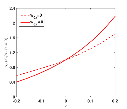
Figure 2: KA slope $\alpha_{\vec{K}}$ as a function of strain. The data are normalized with respect to the value of $\alpha_{\vec{K}}$ for the unstrained graphene ($\epsilon=0$). The solid line corresponds to the deformed Dirac cones including anisotropy and tilt effects while the dashed one is calculated for the untilted cones ($w_{0x}=0$ in Eq.11). The phonon wave vector ${}_{v}ec{q}$ is along the $x$ axis ($\varphi=0$).

According to Fig.2, the KA becomes more pronounced for tensile deformation. $\alpha_{\vec{K}}$ increases of about $20\%$ ($50\%$) for a strain of $5\%$ ($10\%$). However, a compressive deformation reduces the KA slope. This behavior can be understood from the electronic band structure given by Eq.11.

Let us, first, disregard the tilt parameter $w_{0x}$. The shape of the Dirac cones depends on the electron velocities $v_{x}=\frac{w_{x}}{\hbar}\sim v_{F}\left(1+\frac{2}{3}\epsilon\right)$ and $v_{y}=\frac{w_{y}}{\hbar}\sim v_{F}\left(1-\frac{4}{3}\epsilon\right)$ (Eq.10) where $v_{F}$ is the Fermi velocity in the unstrained lattice mark2008 . Therefore, the electron velocity $v_{y}$ ($v_{x}$) along (perpendicular to) the strain direction decreases (increases) with the tensile deformation.

We consider the phonon mediated intervalley electron scattering at a constant energy $E_{L}$ close to the Dirac points, as in the case of the double resonance Raman peak 2D, for which $E_{L}$ is the light excitation energy frank11 ; Narula ; Popov . For unstrained graphene, the momentum cutoff $k_{m}$ in equation 31 could be related to $E_{L}$ as $E_{L}\sim\hbar v_{F}k_{m}$. Regarding the deformed Brillouin zone and the distorted Dirac cones, the intervalley processes become anisotropic.

Figure 3 shows that, for a tensile strain, the number of electron-hole pairs involved in the intervalley scatterings is enhanced (reduced ) along the $y$ ($x$) axis compared to the undeformed lattice. Actually, this anisotropic scattering is schematically equivalent to excite an electron form the $\pi$ band, of the unstrained lattice, with a higher (lower) energy along the $k_{y}$ ($k_{x}$) axis.

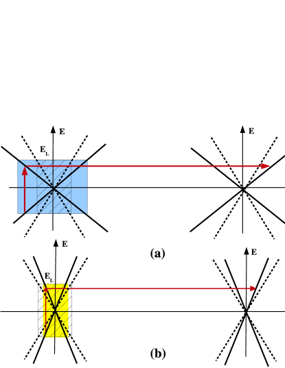
Figure 3: Schematic representations of the intervalley phonon-mediated electronic transitions along the $k_{y}$ (a) and $k_{x}$ (b) axises at a given excitation energy $E_{L}$. The dashed (solid) lines represent the Dirac cones of the unstrained (strained) graphene. The Fermi velocity $v_{y}$ ($v_{x}$) along (perpendicular) to the strain direction $(y^{\prime}y$) is reduced (enhanced) compared to isotropic case. This leads to more (less) electron-hole pairs contributing to the intervalley processes. The colored and dashed areas give the extension of the electronic states contributing to the intervalley transitions around respectively anisotropic and isotropic Dirac cones.

The tensile renormalization of $v_{y}$ is more pronounced than that of $v_{x}$, which means that globally, the area of the electron wave vector $\vec{k}$ delimited by the equi-excitation energy contour $E_{L}$ is larger than that in unstrained graphene, which furthers the electron-phonon scatterings and enhances the KA slope $\alpha_{\vec{K}}$, as shown in Fig.2.

For a compressive strain, the electron-phonon interaction is reduced since the deformation affects much more the processes along $y$ axis, for which the number of created electron-hole pairs is reduced regarding the strain induced enhancement of the electron velocity $v_{y}$.

Let us, now, discuss the role of the Dirac cone tilt. According to Fig.2, the KA for a tensile strain is more marked in the presence of the tilt while it is reduced for a compressive deformation. To explain this behavior, we plot in figure 4 the electronic dispersion, given by Eq.11, along the $k_{x}$ axis, around the Dirac points in the direction $DMD^{\prime}$ for unstrained graphene and deformed lattices under a tensile ($\epsilon=0.2$) and a compressive deformation ($\epsilon=-0.2$). The positions and the shape of the deformed Dirac cones are determined using the whole band structure of the quinoid lattice mark2008 . The Dirac cones move towards each other (away) under a compressive (tensile) deformation MarkRev

Figure 4: Dirac cones in strained graphene ((a) and (c)) and in undeformed lattice (b). The colored axis give the tilt direction of the Dirac cone compared to the untilted case (dashed axis). Under a tensile (compressive) deformation, the Dirac cones, along $DMD^{\prime}$ direction, are tilted towards the $\Gamma$ ($M$) point.

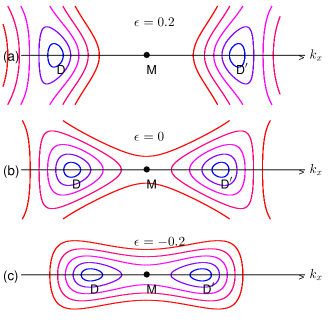
Figure 5: Iso-energy contours along the $k_{x}$ axis for strained (a), (c) and undeformed (b) graphene.

The corresponding iso-energy contours are depicted in Fig.5 showing that, along the $DMD^{\prime}$ direction, the curvature of the these contours is more affected for the outer (inner) electronic states under a tensile (compressive) deformation. By outer and inner states we refer respectively to the states connected by a phonon wave vectors $q_{out}>k_{D}$ and $q_{in}<k_{D}$. For reasons of clarity, we, schematically, represented in figure 6 the band structure depicted in Fig.4 (a).

For a tensile deformation, the outer states are in the tilting direction of the Dirac cones as shown in Fig.6, where we set $k^{0}_{x}$ the electron wave vector corresponding the excitation energy $E_{L}$ in the non-tilted case, namely: $E_{L}=w_{x}k^{0}_{x}$. We denote by $k^{t}_{x,1}$ and $k^{t}_{x,2}$ the wave vectors ascribed to the tilted cone in the D valley ($\xi=+1$ in Eq.11) given by:

$$E_{L}=(w_{0x}+w_{x})k^{t}_{x,1},\,\,E_{L}=(w_{x}-w_{0x})k^{t}_{x,2}$$ (37)

with $w_{0x}\sim 0.6\,\epsilon\,w_{x}$ (Eq.11).

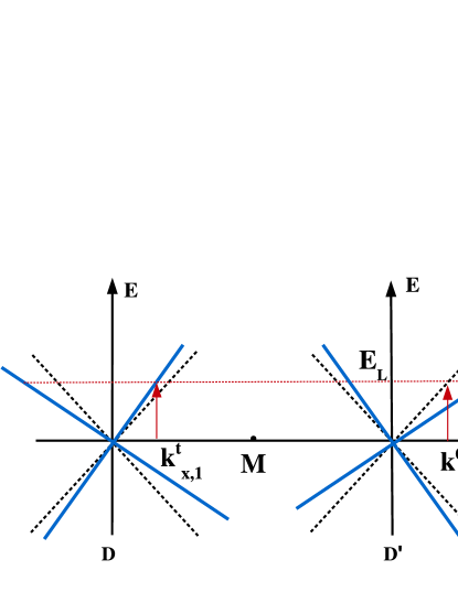
Figure 6: Intervalley phonon-mediated electronic transitions along the $k_{x}$ direction under a tensile deformation and at the excitation energy $E_{L}$ indicated by the red dashed line. The dashed cones represent the nontilted case with a Fermi velocity $v_{x}$ while the blue cones have also the same velocity $v_{x}$ but are tilted due to the term $w_{0x}$ in Eq.11. $k^{0}_{x}$, $k^{t}_{x,1}$ and $k^{t}_{x,2}$, indicated by the arrows, are the electronic states of, respectively, the unstrained and deformed lattices corresponding to the excitation energy $E_{L}$.

The area of the equi-energy contour increases for the tilted cone since $k^{t}_{x,2}-k^{0}_{x}>k^{t}_{x,1}-k^{0}_{x}$, which gives rise to an enhanced number of electron-hole pairs. As a consequence, the electron-phonon interaction increases, which yields to the enhancement of the KA parameter $\alpha_{\vec{K}}$. It is worth to note that the electronic states along the $k_{y}$ axis are not affected by the tilt of Dirac cones.

According to Fig.6, this enhancement is due to the so-called outer intervalley processes involving phonons with wave vectors $q_{out}>k_{D}$. The dominance of the inner or outer processes in the double resonance 2D Raman peak has been a hot topic of debate. Early experimental and numerical studies have argued that the outer phonons contribute mostly to the uniaxial strain induced splitting of the 2D mode Ferrari06 ; Thomsen00 ; Kurti . This outcome was controverted by later findings based on numerical calculations and highlighting the dominance of the inner processes Huang ; Mohr ; Son . Narula et al.Narula have revoked the dominance of both type of phonons and showed, through a numerical study, that the dominant phonon wave vector is highly anisotropic and the distinction between inner and outer processes is irrelevant. It is worth to stress that the above mentioned numerical calculations take into account the strain induced change of the phonon dispersion which is not included in the present work. Our result shows that, the tensile modified electronic dispersion, gives rise to a dominance of the outer phonons in the electron-phonon interaction process and this dominance is due to the tilt of Dirac cones.

On the other hand, Narula et al.Narula have found that the splitting of the 2D peak under a uniaxial tensile strain cannot originate only from the shift of the Dirac points. This result is in agreement with our work showing that the number of the electron-hole pairs involved in the electron-phonon interaction process is independent of the Dirac cone position. This process depends basically on the shape of the equi-excitation energy contours governed by the parameters $w_{x}$ and $w_{y}$ and the tilt factor $\vec{w_{0}}$ (Eq.11).

The strain dependence of the KA depicted in figure 2 could shed light on the anisotropic mechanical properties of strained graphene. Ni et al. PhysicaB have reported, based on molecular dynamics models, that the AC tensile deformation causes the fracture of graphene sooner than a tensile applied along the zigzag (ZZ) edge. This anisotropic behavior was ascribed, by the authors, to different changes of the C-C bond angles. A larger critical strain along the ZZ axis was also reported in Refs.Gao, ; Polymer, .

In the following, we show that the KA could be responsible of the anisotropic failure mechanism of the graphene sheet.

In figure 7, we depicted a schematic representations of the lattice deformed under AC and ZZ tensile where $t$ denote the hopping integral, between first neighbors in unstrained system, and $t^{\prime}$ ($t^{\prime}_{ZZ}$) is the hopping integral under an AC (ZZ) tensile.

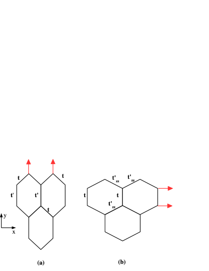
Figure 7: Deformed honeycomb lattice under a tensile applied along the armchair direction (a) and zigzag one (b). The arrows indicate the direction of the tensile deformation. $t$, $t^{\prime}$ and $t^{\prime}_{ZZ}$ are the hopping integrals between first neighboring atoms.

The lattice deformed under a ZZ tensile could be regarded as that obtained under a compressive AC strain with unstrained hopping $\tilde{t}=t^{\prime}_{ZZ}$ and a strain modified hopping integral $\tilde{t}^{\prime}=t$ with $\tilde{t}^{\prime}=\tilde{t}(1+2|\epsilon|)$ (Eq.8). The corresponding KA slope is that given by equation 31 by changing $t$ by $\tilde{t}$ and ${t}^{\prime}$ by $\tilde{t}^{\prime}$.

As shown in figure 2, the KA is reduced, under a compressive strain, compared to the undeformed case ($\epsilon=0$). Moreover, changing $t$ by $\tilde{t}=t^{\prime}_{ZZ}<t$ in Eq.31, reduces the prefactor term and then weakens the KA. As a consequence, the KA is reduced for a ZZ tensile strain compared to the AC one. This result is consistent with the anisotropic frequency shifts of the TO phonon mode under strain along ZZ and AC directions obtained within first-principles calculations in Ref.Bohnen16, We then ascribe the relatively large critical strain along the ZZ edges to the hardening of the TO phonon modes at K point induced by the weakening of the KA. This interpretation is different from that deduced from molecular dynamics calculations ascribing such behavior to the orientation of the C-C bonds with respect to the applied force direction Gao .

It is worth to note, that the lattice softening, resulting from the enhancement of the KA under tensile uniaxial strain, could be counterbalanced by charge doping as reported by Si et al. Si . The authors have found a peculiar behavior of the doping induced frequency shifts of the TO modes at $K$ point. In strained graphene, this shift is remarkably greater than that in unstrained lattice. The authors mentioned that the origin of this large difference is not clear within the framework of their first-principles calculations. In the next, we give, based on schematic representations of the doped graphene band structure, a possible interpretation of this feature.

Figure 8 (a) shows the electron-hole pairs involved in the intervalley phonon-mediated processes in unstrained graphene for a given excitation energy $E_{L}$ and at charge neutrality. By electron doping at $E_{F}<E_{L}$ (Fig.8 (b)), the number of the electron-hole pairs, contributing to the intervalley processes, is reduced due to Pauli principle, which explains the hardening of the phonon frequency by doping unstrained graphene Si .

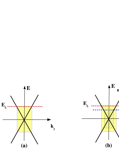
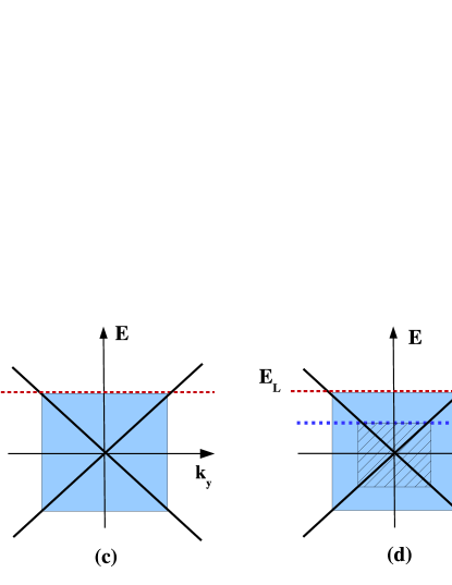
Figure 8: Schematic representation of the electronic states along $k_{y}$ direction involved in the intervalley phonon-mediated processes for a given excitation energy $E_{L}$. (a) and (c) ((b) and ((d)) show to the undoped (doped) unstrained and strained lattices respectively. $E^{\ast}_{F}$ is the strain-renormalized Fermi energy. The dashed areas correspond to the electronic states blocked by the Pauli principle.

Under a uniaxial tensile, the Fermi energy is renormalized as mark2008

$$E^{\ast}_{F}=E_{F}\left(1-\frac{1}{3}\epsilon\right)$$ (38)

In figure 8, we represented the electronic states involved in the intervalley processes along $k_{y}$ direction which give, as discussed above, a dominant contribution to the KA under a tensile deformation. The number of electronic states blocked by the Pauli principle in the strained lattice is greater than that for undeformed case. Indeed, these states are in the interval $\Delta k_{y}=E^{\ast}_{F}/w_{y}\sim(1+\epsilon)E_{F}/w$ while in the unstrained lattice, the locked states are within the interval $\Delta k^{0}_{y}=E_{F}/w$ where $w=\frac{3}{2}at$ ((Eq.11).

For $\epsilon>0$, $\Delta k_{y}>\Delta k^{0}_{y}$. This leads to a larger number of blocked intervalley processes in graphene under uniaxial tensile strain which is consistent with the result of Ref.Si, . Moreover, the KA is expected to be weakened by doping regarding the enhancement of $\Delta k_{y}$ with $E_{F}$ which is in agreement with Refs. Si, ; Wang17, .

In figure 9 we represent the phonon angle dependence of the normalized KA parameter for different strain values. For the unstrained lattice, the KA is isotropic with respect to the phonon wave vector direction since the iso-energy contours are almost circular at low energy. As the strain amplitude increases, the KA becomes anisotropic with a dominant component for phonons with wave vector $\vec{q}$ along the $x$ axis which is perpendicular to the strain direction.

This result is in agreement with the light polarization angle dependence of the 2D Raman band reported in literature. Several experimental and numerical studies Huang ; frank11 ; Popov have found that the 2D peak splits, under strain, into two lines. Under AC strain, the intensity of the line associated to a parallel light polarization, with respect to the strain direction, is greater than that of the peak ascribed to the perpendicular polarization i.e. $I_{2D}(\theta=90^{\circ})<I_{2D}(\theta=0^{\circ})$, where $\theta$ is the angle of the light polarization with the respect to the strain direction Popov . Since the Raman intensity depends on $|\vec{q}\times\vec{E}|$ where $\vec{q}$ is the phonon wave vector and $\vec{E}$ is the light polarization Basko , the 2D band is then expected to show a large intensity for $\vec{q}$ along the direction perpendicular to the strain axis. This behavior is in agreement with our result depicted in figure 9 showing that the KA is enhanced for $\varphi=0$.

Moreover, figure 9 shows that the KA should exhibit a minimum around the $y$ direction ($\varphi=\pi/2$). This behavior is due to the tilt of Dirac cones which, as discussed above, enhances the KA for electronic states along $k_{x}$ axis. According to figure 9, the KA is expected to have a relative maximum for phonons with $\varphi=\pi$, which correspond to the inner intervalley processes. The latter have, as we already shown, have a minor contribution, to the KA, compared to the outer processes.

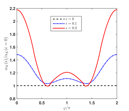
Figure 9: Phonon angle dependence of the KA slope $\alpha_{\vec{K}}$ for different strain amplitudes. $\varphi$ is the angle between the phonon wave vector $\vec{q}$ and the $x$ axis perpendicular to the strain direction. The data are normalized with respect to the value of $\alpha_{\vec{K}}$ for $\varphi=0$ in the unstrained lattice ($\epsilon=0$).

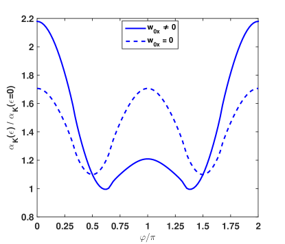
Figure 10: Phonon angle dependence of the KA slope $\alpha_{\vec{K}}$ in the case of titled (solid line) and nontilted (dashed line) cones. The data are normalized with respect to the value of $\alpha_{\vec{K}}$ for $\varphi=0$ in the unstrained lattice.

Figure 10 shows the KA slope as a function of the phonon angle for a tensile strain of $\epsilon=0.2$. T he solid (dashed) curve corresponds to the case of tilted (non-tilted) Dirac cones. According to this figure, the anisotropic behavior of $\alpha_{\vec{K}}$ is due to the anisotropic Fermi velocities of the $v_{x}=w_{x}/\hbar$ and $v_{y}=w_{y}/\hbar$. However, the tilt parameter is responsible of the dominance of the outer intervalley phonon processes, corresponding to $\varphi=0$, for which $\alpha_{\vec{K}}$ reaches its maximum value. The inner processes have a lower contribution associated to $\varphi=\pi$.

As mentioned by Narula et al., the notion of inner and outer processes is rather confusing since they can be mapped into each other by the addition of a reciprocal lattice vector. The authors showed, based on numerical calculations, that the dominant phonon-mediated intervalley electronic transitions are neither inner nor outer but with a significant contribution of the inner processes. To avoid any confusing nomenclature we conclude that the intervalley processes, connecting the most deformed parts of the electronic iso-energy contours, have the dominant contribution to the KA around the Dirac points.

IV Conclusion

In summary, we have presented an analytical study of the effect of the electronic dispersion relation on the KA of strained graphene. We found that, besides the shifts of the KA phonon wave vector, the strain dependence of the slope parameter $\alpha_{\vec{K}}$ describing this anomaly is substantially dependent on the electronic band structure. In particular, the KA is found to be enhanced under tensile strain, by the tilt of Dirac cones. The latter furthers the so-called outer intervalley phonon processes. We have, also, found that the strain dependence of the electronic band structure is at the origin of the strong doping induced reduction of the KA in graphene under a tensile deformation compared to the undeformed lattice. Moreover, our results show that the KA is anisotropic with respect to the phonon wave vector which may give insights not only on light polarization dependence of Raman 2D band but also on the anisotropic mechanical failure of graphene under strain.

V Acknowledgment

We thank M. E. Cifuentes-Quintal for stimulating discussions. We are indebted to M. E. Cifuentes-Quintal, J.- N. Fuchs and Reza Asgari for a critical reading of the manuscript. S. H. acknowledges the kind hospitality of ICTP (Trieste, Italy) where part of the work was carried out. S. H. was supported by Simons-ICTP associate fellowship.

Appendix A EPC Hamiltonian by $\vec{k}.\vec{p}$ method

The $\vec{k}.\vec{p}$ method was used by Suzuura and Ando Ando to obtain the effective Hamiltonian describing the interaction between electrons and the zone boundary optical phonons corresponding to the highest frequency mode, the so-called Kekulé mode. This method was also used to determine the electron-phonon interaction Hamiltonian in the case of the optical center zone phonon modes of graphene in the absence of deformation ando2006 and under a uniaxial strain Assili .

Based on Ref.Ando, , we derive the EPC matrix element $g_{D^{\prime},\vec{k}^{\prime}=\vec{k}+\vec{q},\pi^{\ast};D,\vec{k},\pi}$ corresponding to the transition of an electron from the occupied band ($\pi$) of the valley $D$ to the empty band $\pi^{\ast}$ at the $D^{\prime}$ valley in graphene, under uniaxial strain applied along the armchair direction.

We start with the electronic eigenproblem given by Eq.22 where the functions $\psi_{A}(\vec{R}_{A})$ and $\psi_{B}(\vec{R}_{B})$ can be written in terms of the envelope functions $F_{A}^{D/D^{\prime}}(\vec{R}_{A})$ and $F_{B}^{D/D^{\prime}}(\vec{R}_{B})$ as :

$$\psi_{A}(\vec{R}_{A})=a^{\dagger}(\vec{R}_{A})\Phi_{A}(\vec{R}_{A})$$

$$\psi_{B}(\vec{R}_{B})=b^{\dagger}(\vec{R}_{B})\Phi_{B}(\vec{R}_{B})$$

with

$$a(\vec{R}_{A})=\left(\begin{array}[]{c}\mathrm{e}^{-i\vec{k}^{D}.\vec{R}_{A}}\\ \mathrm{e}^{-i\vec{k}^{D^{\prime}}.\vec{R}_{A}}\end{array}\right)\quad b(\vec{R}_{B})=\left(\begin{array}[]{c}\mathrm{e}^{-i\vec{k}^{D}.\vec{R}_{B}}\\ -\mathrm{e}^{-i\vec{k}^{D^{\prime}}.\vec{R}_{B}}\end{array}\right)$$ (44)

$$\Phi_{A}(\vec{R}_{A})=\left(\begin{array}[]{c}F_{A}^{D}(\vec{R}_{A})\\ F_{A}^{D^{\prime}}(\vec{R}_{A})\end{array}\right)\quad\Phi_{B}(\vec{R}_{B})=\left(\begin{array}[]{c}F_{B}^{D}(\vec{R}_{B})\\ F_{B}^{D^{\prime}}(\vec{R}_{B})\end{array}\right)$$ (49)

As in Ref.Ando, , we introduce the smoothing function $g(\vec{r})$ satisfying the following relations:

$$\sum_{\vec{R}_{A}}g(\vec{r}-\vec{R}_{A})=\sum_{\vec{R}_{B}}g(\vec{r}-\vec{R}_{B})=1$$

$$f(\vec{r})g(\vec{r}-\vec{R}_{A})\simeq f(\vec{R})g(\vec{r}-\vec{R}).$$ (51)

where $f(\vec{r})$ is an envelope functionando2006 . The left-hand side of Eq.22 can then be written, at $\vec{R}_{A}$ site, as:

$$\varepsilon\,a(\vec{R}_{A})a^{\dagger}(\vec{R}_{A})F_{A}(\vec{r}) = \varepsilon\sum_{\vec{R}_{A}}g(\vec{r}-\vec{R}_{A})a(\vec{R}_{A})a^{\dagger}(\vec{R}_{A})F_{A}(\vec{r})=-\sum_{l=1}^{3}t^{(l)}\sum_{\vec{R}_{A}}g(\vec{r}-\vec{R}_{A})a(\vec{R}_{A})b^{\dagger}(\vec{R}_{B})F_{B}(\vec{r}-\vec{\tau}_{l})$$ (52)

$$- \sum_{l=1}^{6}t_{nnn}^{(l)}\sum_{\vec{R}_{A}}g(\vec{r}-\vec{R}_{A})a(\vec{R}_{A})a^{\dagger}(\vec{R}_{A}-\vec{a}_{l})F_{A}(\vec{r}-\vec{a}_{l})$$

For small strain amplitude, the following relations are satisfied:

$$\sum_{\vec{R}_{A}}g(\vec{r}-\vec{R}_{A})\mathrm{e}^{i(\vec{k}^{D^{\prime}}-\vec{k}^{D}).\vec{R}_{A}}=\sum_{\vec{R}_{B}}g(\vec{r}-\vec{R}_{B})\mathrm{e}^{i(\vec{k}^{D^{\prime}}-\vec{k}^{D}).\vec{R}_{B}}\simeq 0$$

$$\sum_{\vec{R}_{A}}g(\vec{r}-\vec{R}_{A})\mathrm{e}^{i\vec{k}^{D}.\vec{R}_{A}}\simeq 0$$ (53)

Taking into account the lattice vibrations on the hopping integral to the first neighbor atoms, an extra term appears in the eigenproblem given by Eq.22. This term is of the form:

$$H_{int}F_{B}(\vec{r})=\sum_{l}\sum_{\vec{R}_{A}}g(\vec{r}-\vec{R}_{A})a(\vec{R}_{A})b(\vec{R}_{A}-\vec{\tau}_{l})\left(-\frac{\partial t^{(l)}}{\partial d_{l}}\right)\left(\frac{\vec{\tau}_{l}}{d_{l}}\right).\left(\vec{u}_{A}(\vec{R}_{A})-\vec{u}_{B}(\vec{R}_{A}-\vec{\tau}_{l})\right)F_{B}(\vec{r})$$ (54)

where $F_{B}(\vec{r})=\left(\begin{array}[]{c}F_{B}^{D}(\vec{r})\\ F_{B}^{D^{\prime}}(\vec{r})\end{array}\right)$.

We consider the phonon modes around the Dirac points $D$ and $D^{\prime}$ with wave vector $\vec{k}^{D/D^{\prime}}+\vec{q}$ where $\|\vec{q}\|\ll\frac{2\pi}{a}$. We can then use the continuum limit and put in Eq.24: $\vec{u}^{D/D^{\prime}}_{A}(\vec{R}_{A})\simeq\vec{u}^{D/D^{\prime}}_{A}(\vec{r})$ and $\vec{u}^{D/D^{\prime}}_{B}(\vec{R}_{A}-\vec{\tau}_{l})\simeq\vec{u}^{D/D^{\prime}}_{B}(\vec{r})$. Equation 54 can then be written as:

$$H_{int}F^{D}_{B}(\vec{r})=h^{\prime AB}_{int}F^{D^{\prime}}_{B}(\vec{r})$$ (55)

where $h^{\prime AB}_{int}$ is given by:

$$h^{\prime AB}_{int}=\sum_{l}\left(-\frac{\partial t^{(l)}}{\partial d_{l}}\right)\left(\frac{\vec{\tau}_{l}}{d_{l}}\right).\left[\mathrm{e}^{-i\vec{k}^{D^{\prime}}.\vec{\tau}_{l}}\vec{u}^{D^{\prime}}_{A}(\vec{r})-\mathrm{e}^{-2i\vec{k}^{D^{\prime}}.\vec{\tau}_{l}}\vec{u}^{D^{\prime}}_{B}(\vec{r})\right]$$

with $t^{(1)}=t^{(2)}=t$, $t^{(3)}=t^{\prime}=t(1-2\epsilon)$, $\vec{k}^{D^{\prime}}.\vec{\tau}_{3}=0$, and $\vec{k}^{D^{\prime}}.\vec{\tau}_{1}=-\vec{k}^{D^{\prime}}.\vec{\tau}_{2}=-\theta$, where $\theta=\arccos\left(-\frac{t^{\prime}}{2t}\right)=a\frac{\sqrt{3}}{2}k^{D}_{x}$.

$h^{\prime AB}_{int}$ takes then the following form:

$$h^{\prime AB}_{int} = -i\frac{3a}{2}\frac{1}{b}\frac{\partial t}{\partial b}\left[\left(1+\frac{2}{3}\epsilon\right)u^{D^{\prime}}_{Ax}(\vec{r})+iu^{D^{\prime}}_{Ay}(\vec{r})\right.$$ (57)

$$+ \left.\left(1-\frac{4}{3}\epsilon\right)u^{D^{\prime}}_{Bx}(\vec{r})-i\left(1+2\epsilon\right)u^{D^{\prime}}_{By}(\vec{r})\right]$$

where we considered the limit of small strain amplitude ($|\epsilon|\ll 1$).

To bring out the signature of the electronic dispersion on the EPC, we assume that the phonon dispersion at $K^{\prime}$ point is not affected by the strain. This means that the phonon polarization of the highest frequency optical mode is Ando $\vec{e}_{D^{\prime}}=\vec{e}_{K^{\prime}}=\frac{1}{2}=\left(\begin{array}[]{c}1\\ -i\\ 1\\ i\end{array}\right)$.

The matrix element $h^{\prime AB}_{int}$ becomes:

$$h^{\prime AB}_{int} = -3ai\frac{1}{a}\frac{\partial t}{\partial a}\left(1+\frac{1}{3}\epsilon\right)\vec{e}_{D^{\prime}}^{\;0}.\vec{U}_{D^{\prime}}$$

where

$$\vec{U}_{D^{\prime}}=\left(\begin{array}[]{c}\vec{u}^{D^{\prime}}_{A}\\ \vec{u}^{D^{\prime}}_{B}\end{array}\right)=\sqrt{\frac{\hbar}{2NM\omega_{K}}}\vec{e}_{K^{\prime}}\sum_{\vec{q}}\left(b_{D,\vec{q}}+b^{\dagger}_{D,-\vec{q}}\right)\mathrm{e}^{i\vec{q}.\vec{r}}$$ (61)

and $\vec{e}_{D^{\prime}}^{\;0}=\frac{1}{2\left(1+\frac{1}{3}\epsilon\right)}\left(\begin{array}[]{c}1+\frac{2}{3}\epsilon\\ -i\\ 1-\frac{4}{3}\epsilon\\ i(1+2\epsilon)\end{array}\right)$.

The effective interaction Hamiltonian takes a form similar to that found by Suzzura and Ando Ando :

$$H_{int}=-3\frac{t}{a}\beta_{K}\left(1+\frac{1}{3}\epsilon\right)\left(\begin{array}[]{cc}0&\Delta_{D^{\prime}}\sigma_{y}\\ \Delta_{D}\sigma_{y}&0\end{array}\right)$$ (65)

with $\Delta_{D^{\prime}}=\vec{e}_{D^{\prime}}^{\;0}.\vec{U}_{D^{\prime}}$, $\beta_{K}=-\frac{b}{t}\frac{\partial t}{\partial b}$ and $\sigma_{y}$ is the Pauli matrix.

^∗ Electronic address: sonia.haddad@fst.rnu.tn

References

- (1) A. H. Castro Neto, F. Guinea, N. M. R. Peres, K. S. Novoselov, and A. K. Geim, Rev. Mod. Phys. 81, 109 (2009).
- (2) M. S. Nevius, M. Conrad, F. Wang, A. Celis, M. N. Nair, A. Taleb-Ibrahimi, A. Tejeda, and E. H. Conrad, Phys. Rev. Lett. 115, 136802 (2015).
- (3) V. N. Kotov, B. Uchoa, V. M. Pereira, F. Guinea and A. H. Castro Neto, Rev. Mod. Phys. 84, 1067 (2012).
- (4) G. Naumis, S. Barraza-Lopez, M. Oliva-Leyva and H. Terrones, Rep. Prog. Phys. 80 096501 (2017).
- (5) C. Si, Z. Suna and F. Liu, Nanoscale, 8, 3207 (2016).
- (6) R. Roldán, A. Castellanos-Gomez, E. Cappelluti and F. Guinea, J. of Phys.: Condensed Matter, 27, 313201 (2015).
- (7) M. A. Bisset, M. Tsuji and H. Ago, Phys. Chem. Chem. Phys. 16 11124 (2014).
- (8) F. Guinea, Solide State Comm. 152, 1437 (2012).
- (9) V. M. Pereira and A. H. Castro Neto and N. M. R. Peres, Phys. Rev. Lett. 103, 046801 (2009).
- (10) C. Si, Z. Suna and F. Liu, Nanoscale, 2016, 8, 3207 (2015).
- (11) N. Levy, S.A. Burke, K.L. Meaker, M. Panlasigui, A. Zettl, F. Guinea, A. H. Castro Neto, M. F. Crommie, Science 329, 544 (2010).
- (12) C. Si, Z. Liu, W. Duan, and F. Liu, Phys. Rev. Lett. 111, 196802 (2013).
- (13) B. Uchoa and Y. Barlas, Phys. Rev. Lett. 111, 046604 (2013).
- (14) C. Lee, X. Wei, J. W. Kysar and J. Hone, Science 321 385 (2008).
- (15) V. M. Pereira, A. H. Castro Neto and N. M. R. Pere, Phys. Rev. Lett. 80, 045401 (2009).
- (16) N. Z. Hua, Y. Ting, L. Y. Hao, W. Y. Ying, F. Y. Ping and S. Z. Xiang, ACS Nano 3 483 (2009).
- (17) F. Guinea, M. I. Katsnelson and A. K. Geim, Nature Physics, 6, 30 (2010).
- (18) C-L. Li, AIP Advances 4 087119 (2014).
- (19) A. C. Ferrari, and D. M. Basko, Nature Nanotechnology, 8, 235 (2013).
- (20) M. Huang, H. Yan, T. F. Heinz, and J. Hone, Nano Lett. 10, 4074-4079 (2010).
- (21) Z. H. Ni, W. Chen, X. F. Fan, J. L. Kuo, T. Yu, A. T. S. Wee, and Z. X. Shen, Phys. Rev. B 77, 115416 (2008).
- (22) Z. H. Ni, T. Y, Y. H. Lu, Y. Y. Wang, Y. P Feng, and Z. X. Shen, ACS Nano, 2, 2301 (2008).
- (23) T. M. G. Mohiuddin, A. Lombardo, R. R. Nair, A. Bonetti, G. Savini, R. Jalil, N. Bonini, D. M. Basko, C. Galiotis, N. Marzari, K. S. Novoselov, A. K. Geim, and A. C. Ferrari, Phys. Rev. B 79, 205433 (2009).
- (24) O. Frank, G. Tsoukleri, J. Parthenios, K. Papagelis, I. Riaz, R. Jalil, K. S. Novoselov, and C. Galiotis, ACS Nano 4, 3131 (2010), O. Frank, G. Tsoukleri, I. Riaz, K. Papagelis, J. Parthenios, A. C. Ferrari, A. K. Geim, K. S. Novoselov and C. Galiotis, Nature Communications 2, 1247 (2011).
- (25) O. Frank, M. Mohr, J. Maultzsch, C. Thomsen, I. Riaz , R. Jalil, K. S. Novoselov, G. Tsoukleri, J. Parthenios, K. Papagelis, L. Kavan, and C. Galiotis, ACS Nano, 5 2231 (2011).
- (26) J.-U. Lee, D. Yoon, and H. Cheong, Nano Lett. 12 4444 (2012).
- (27) C. W. Huang, R. J. Shiue, H. C. Chui, W. H. Wang, J. K. Wang, Y. Tzeng, and C. Y. Liu, Nanoscale, 5, 9626 (2013).
- (28) D. Yoon, Y. W. Son, and H. Cheong, Phys. Rev. Lett. 106, 155502 (2011).
- (29) V. N. Popov, and P. Lambin, Carbon 54, 86 (2013), V. N. Popov, P. Lambin, Phys. Rev. B 87 155425 (2013).
- (30) C. Thomsen, S. Reich, and P. Ordejón, Phys. Rev. B 65, 03403 (2002)
- (31) M. Mohr, J. Maultzsch, and C. Thomsen, Phys. Rev. B 82, 201409(R) (2010).
- (32) R. Narula, N. Bonini, N. Marzari, and S. Reich, Phys. Rev. B 85, 115451 (2012).
- (33) M. Assili, and S. Haddad, Phys. Rev. B. 90, 125401 (2014).
- (34) C. Neumann, S. Reichardt, P. Venezuela, M. Drögeler, L. Banszerus, M. Schmitz, K. Watanabe,T. Taniguchi, F. Mauri, B. Beschoten, S.V. Rotkin and C. Stampfer, Nat. Commun. 6 8429 (2015).
- (35) X. Wang, J. W. Christopher and A. Swan, Sci. Rep., 7, 13539 (2017).
- (36) S. Reich, C. Thomsen Philos. Trans. R. Soc. A 362 2271 (2004).
- (37) C. Thomsen and S. Reich, Phys. Rev. Lett. 85, 5214 (2000).
- (38) D. M. Basko, Phys. Rev. B 78, 125418 (2008).
- (39) R. Saito, A. Jorio, A. G. Souza Filho, G. Dresselhaus, M. S. Dresselhaus, and M. A. Pimenta, Phys. Rev. Lett. 88, 027401 (2001).
- (40) J. Maultzsch, S. Reich, and C. Thomsen, Phys. Rev. B 70, 155403 (2004).
- (41) P. Venezuela, M. Lazzeri, and F. Mauri, Phys. Rev. B 84, 035433 (2011).
- (42) W. Kohn, Phys. Rev. Lett. 2, 393 (1959).
- (43) S. Piscanec, M. Lazzeri, Francesco Mauri, A. C. Ferrari, and J. Robertson, Phys. Rev. Lett. 93, 185503 (2004).
- (44) M. Lazzeri and F. Mauri, Phys. Rev. Lett. 97, 266407 (2006).
- (45) M. Lazzeri, C. Attaccalite, L. Wirtz, and F. Mauri, Phys. Rev. B 78, 081406(R) (2008).
- (46) K. Sasaki, M. Yamamoto, S. Murakami, R. Saito, M. S. Dresselhaus, K. Takai, T. Mori, T. Enoki, and K. Wakabayashi, Phys. Rev. B 80, 155450 (2009).
- (47) S. K. Saha, U. V. Waghmare, H. R. Krishnamurthy and A. K. Sood, Phys. Rev. B 76, 201404(R) (2007), F. Forster, A. Molina-Sanchez, S. Engels, A. Epping, K. Watanabe, T. Taniguchi, L. Wirtz, and C. Stampfer, Phys. Rev. B 88, 085419 (2013), F. de Juan and H. A. Fertig, Phys. Rev. B 85, 085441 (2012).
- (48) C. A. Marianetti and H. G. Yevick, Phys. Rev. Lett. 105, 245502 (2010).
- (49) C. Si, W. Duan, Z. Liu, and F. Liu, Phys. Rev. Lett. 109, 226802 (2012).
- (50) M. E. Cifuentes-Quintal, O. de la Peña-Seaman, R. Heid, R. de Coss, and K.-P. Bohnen, Phys. Rev. B 94, 085401 (2016).
- (51) V. M. Pereira, A. H. Castro Neto, and N. M. R. Peres, Phys. Rev. B 80, 045401 (2009).
- (52) F. Liu, P. Ming, J. Li, Phys. Rev. B 76, 064120 (2007).
- (53) H. Zhao, K. Min, and N. R. Aluru, Nano Lett. 9, 3012 (2009).
- (54) Y. Gao, P. Hao, Physica E, 41, 1561 (2009).
- (55) Z. Ni, H. Bu, M. Zou, H. Yi, K. Bi, Y. Chen, Physica B, 405, 1301 (2010).
- (56) G. Cao, Polymers, 6, 2404 (2014).
- (57) Y. I. Jhon, Y. M. Jhon, G. Y. Yeom, M. S. Jhon, Carbon, 66, 619 (2014).
- (58) M. O. Goerbig, J.-N. Fuchs, and G. Montambaux, F. Piéchon, Phys. Rev. B, 78, 045415 (2008).
- (59) M. Goerbig, Rev. Mod. Phys. 83, 1193 (2011).
- (60) M. E. Cifuentes-Quintal, private communication.
- (61) Y. Betancur-Ocampo, M.E. Cifuentes-Quintal, G. Cordourier-Maruri, R. de Coss, Annals of Physics 359 243 (2015).
- (62) A. Kobayashi, S. Katayama, Y. Suzumura, and H. Fukuyama, J. Phys. Soc. Jpn. 76 034711 (2007).
- (63) H. Suzuura and T. Ando, J. Phys. Soc. Jpn. 77 044703 (2008).
- (64) T. Ando, J. Phys. Soc. Jpn. 75, 084713 (2006).
- (65) P. Marconcini, and M. Macucci, Rivista del Nuovo Cimento, 34, 489 (2011).
- (66) A. C. Ferrari, J. C. Meyer, V. Scardaci, C. Casiraghi, M.Lazzeri, F. Mauri, S. Piscanec, D. Jiang, K.S. Novoselov, S. Roth , and A. K. Geim, Phys. Rev. Let. 97, 187401 (2006).
- (67) J. Kurti, V. Zolyomi, A. Gruneis, and H. Kuzmany, Phys. Rev. B 65, 165433 (2002).