Fractional Quantum Hall Effect in Landau Band of Graphene
with Chern Number Matrix
Koji Kudo1 and Yasuhiro Hatsugai1,21Graduate School of Pure and Applied Science1Graduate School of Pure and Applied Science University of Tsukuba University of Tsukuba Tsukuba 305-8571 Tsukuba 305-8571 Japan
2Division of Physics Japan
2Division of Physics University of Tsukuba University of Tsukuba Tsukuba Tsukuba Ibaraki 305-8571 Ibaraki 305-8571 Japan Japan
Abstract
Fully taking into account the honeycomb lattice structure, fractional
quantum Hall states of graphene are considered by a pseudopotential projected
into the Landau band. By using chirality as an internal degree of
freedom, the Chern number matrices are defined and evaluated numerically.
Quantum phase transition induced by changing a range of the interaction is
demonstrated that is associated with chirality ferromagnetism. The
chirality-unpolarized ground state is consistent with the Halperin 331 state of
the bilayer quantum Hall system.
The concept of topological order
[1, 2, 3] substantially expands our understanding of phases of
matter that cannot be described by the conventional order parameters
associated with symmetry breaking. The quantum Hall effect
[4, 5] is a prominent example
of topologically non-trivial quantum phases. The quantized Hall conductance is
expressed as the Chern number
[6, 7, 8]
associated with the Berry connection[9]. Although the integer
quantum
Hall state can be described by non-interacting electrons, the
electron-electron interaction plays a crucial role in the fractional quantum
Hall (FQH) phase. The characteristics of these correlated quantum states are
well captured by the Laughlin wave function[10]. In
addition,
its excitations are quasiparticles with fractional
charges and fractional statistics[11]. This FQH effect
is understood as an integer quantum Hall effect of composite fermions as flux
charge composites [12]. It also provides a consistent
picture
at an even-denominator Landau level (LL) filling [13].
The internal degrees of freedom, such as spin or layer index, bring further
diversity to the FQH phases. The ground state at
[14] is described by the Moore-Read
Pfaffian state [15] with the excitation obeying
non-Abelian statistics [16] when the interaction is
short-range. As for two-component Abelian FQH systems, the Halperin
state [17] is a typical example. This is realized in a
bilayer FQH system at [18, 19, 20, 21, 22, 23], for example, but its
appearance depends strongly on the system parameters. For
multi-component systems, the symmetric integer matrix
[24, 25, 26, 27]
provides classification of the FQH phases, which is discussed in relation to
the Chern number matrix [28, 29].
The FQH effect of graphene [30, 31, 32, 33, 34] is also an example of the
multi-component FQH systems. The low-energy behavior of electrons in graphene
is
described by the doubled massless Dirac fermions at and points in the
Brillouin zone. These characteristics give rise to the FQH
phases peculiar to graphene.
[35, 36, 37, 38, 39, 40, 41, 42, 43, 44, 45].
Since the LL is a standard lowest LL of the valley polarized Dirac
fermions, the FQH effect of the LL has been discussed similarly with the
SU(2) invariance arising from the valley degree of freedom. The ground states
at the LL filling factor and are described by the
pseudospin (valley) polarized Laughlin state and pseudospin singlet composite
fermion Fermi sea, respectively.
[36, 37]
In this study, the FQH system for the Landau band is investigated
by fully taking into account the honeycomb lattice structure of the
interaction. Short-range
electron-electron interaction of the nearest neighbor (NN) and next-nearest
neighbor (NNN) is
discussed in this paper by constructing the pseudopotential
[46]
projected into the Landau band. The chiral symmetry of the honeycomb
lattice plays an important role in the many-body problems as well
[47, 48, 49].
The quantum phase transitions associated with the chirality ferromagnetism
occur by changing the interaction range. Since the total pseudospin is not
conserved because of the lattice effects, the SU(2) symmetry discussed by the
continuous approximation is absent. In order to characterize
the quantum phases topologically, the Chern number matrices specified by the
chiral basis are constructed numerically. The results are also discussed in
relation to the conventional bilayer quantum Hall system.
Let us begin by introducing the projected fermion operators into
the Landau band. Here, we assume that the system is always
spin-polarized. The kinetic Hamiltonian is written as
(1)
which describes hopping between the NN pairs of sites with
strength . Here, , and
creates a fermion at the sublattice for unit cell .
The Peierls phase is determined such that the sum of the phases
around an elementary hexagon is equal to the magnetic flux in units
of the flux quantum . In the calculation, the string gauge
[50, 51] is employed,
which enables us to realize the minimum magnetic fluxes that are consistent
with the lattice periodicity. When the system is put on the
unit cells with a periodic boundary condition, the magnetic field can be
provided as ,
where . Here, corresponds to the total magnetic
flux. The lattice model with ( relatively prime) has
single-electron bands, where 2 comes from the sublattice degree of freedom.
The number of states per band is obtained as . For the weak magnetic
field (), bands flow into each other around the zero energy, which
form the LL in the large limit. Thus, in this paper, “the
Landau band” is defined as a group of these bands, where there are
one-body states.
Since the honeycomb lattice is bipartite, the Hamiltonian has
chiral symmetry. The matrix
anticommutes with
the Hamiltonian as and . If is the eigenvector of with the energy
, the chiral symmetry guarantees that is identical
to the one with . Thus, the chiral operator can be
diagonalized within the one-body states of the Landau band. Then, the
chiral basis can be defined as ,
, and
. Note that is localized on
the sublattice so that the multiplet can be expressed as
,
where is a proper matrix
[49].
Next, let us consider the two-body interactions written as
(2)
where and
is the strength of the electron-electron interaction.
In order to construct the pseudopotential, the projected creation-annihilation
operators are defined as
[47, 48, 49, 51], where . This expression is
simplified by writing and
.
Note that these projected operators no longer satisfy the canonical
anticommutation relations (). By taking into account the ordering of fermions,
the replacement of , with ,
causes the Hamiltonian to be projected into the Landau
band. Then, the projected Hamiltonian can be defined as
(3)
(4)
where
, and . Here, we choose the strength of the interaction such
that its energy scale is much larger than the energy width of the Landau
band, so that only the interaction term is considered. The projected
Hamiltonian commutes with the total chirality operator
written as
(5)
which enables us to classify the -body states by the total
chirality
. Now, the filling
factor is defined as .
Hereafter, we consider the electron-electron interaction between
NN and NNN pairs,
(6)
where and are the strength of the interaction. Note that the
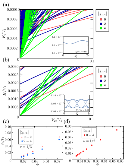
interaction () contributes ( and ). Figures 1 (a) and (b)
show the dependence of the four-electron energy obtained by the
exact diagonalization at and .
Since the exact topological degeneracy due to the
center-of-mass translation [52] is given by the Landau
gauge in a finite system, we choose a system of size for
as shown in Fig. 1 (a) at . For example, the
chirality-polarized ground state multiplet is exactly three-fold degenerated.
(See the inset in Fig. 1 (a).) As for the system at , to
be compatible to the Dirac cones at and points of graphene, the system
size should be (). Then, we choose the magnetic flux
as using the string gauge. In this case, the
topological degeneracy is not exact. However, the energy separation of the
entangled states within the ground state multiplet is very small. For example,
it is less than 0.003 times the energy gap for the six-fold ground state
multiplet with .
(See the inset in Fig. 1 (b).)
Note that the magnetic length ,
where is the area of the elementary hexagon with lattice
constant , is approximately and for and ,
respectively.
Figure 1: (Color online) (a, b) Many-body spectrum as a function of the ratio
at filling factor (a) and (b) .
The total chiralities are expressed by the line colors.
The insets show the many-body spectra with
for . The horizontal axis is the
twist (). (See Eq. (7).)
Note that the level crossing in the inset of (b) is not exact.
(c, d) Dependence of the phase transition point on
magnetic flux at (c) and (d) .
The transition point denoted as - indicates the transition between
and .
In the case of , that is, only the bipartite interactions,
many-body states with should be eigenstates with
zero eigenvalues. Generally, the system at
provides -fold degenerate ground states
(2 comes from the sign of chirality), which are lifted by the infinitesimal
. Further, an increase in leads the phase transition from to since the NNN interactions act between the same
sublattices. In Fig. 1 (c) and (d), the ratio
at the phase transition points is plotted against the magnetic flux
at and .
The results suggest that the
strong short-range interaction compared with the magnetic flux ()
favors the unpolarized chirality unless is not vanishing.
Since the pseudopotential is constructed on the basis of the honeycomb lattice
model,
only the -component of the pseudospin, , is conserved. The
SU(2) symmetry arising from the chirality is absent in contrast to the cases
in the continuum limit [36, 37]. Then,
in order to investigate the internal topological structure of
the many-body states, we evaluate the Chern number matrices associated with the
chirality. First, we investigate the twisted boundary condition
[7],
and
, where and
are the labels of the unit cell for the and directions. Since the
chiral symmetry remains in the kinetic Hamiltonian , the connection between chirality and sublattice is preserved.
Let us consider each projected fermion operator
and with different twisted boundary conditions,
(7)
where . The projected Hamiltonian can be defined by replacing
with in
Eq. (3). Note that this Hamiltonian can be written by the fermion
operators ,
which satisfy the canonical anticommutation relations
for any .
Now, let us further define the non-Abelian Berry connection and curvature
[9, 2, 3]
of the -fold ground state multiplet by selecting the sublattices in each direction as
(8)
(9)
where , and the two parameters except for
and are fixed to 0. Then, the Chern
number matrix is defined as
(12)
The element is evaluated as
[53, 51]
numerically, where
,
,
, and
represents the lattice displacement in the
direction for the sublattice .
In order to construct the ground state multiplet
numerically, a basis of -electron states classified by the total
chirality is defined as
.
Here, is the dimension of the Hilbert space, and
(13)
where is one of the possible ways to occupy states by
electrons, and . Then, the
ground state multiplet is expressed as , where , and is the eigenvector of
. We have
and
where
,
is the -th column vector of , and .
We first focus on the chirality-polarized states with for . Since the polarized many-body states occupy only
the sublattice , the staggered sublattice potential written as
stabilizes the polarized many-body states. Now, the ground
state multiplet is defined as a group of lowest-energy many-body states that is
separated from the other excited states. Numerically obtained ground
states at and are similar to those
provided by the pseudopotentials projected into the lowest Landau band
[51].
At , the ground state is always three-fold degenerated
irrespective of the number of electrons. This three-fold ground state multiplet
is gapped in the thermodynamic limit similar to the
Ref. \citendoi:10.7566/JPSJ.86.103701. In addition, its Chern number
is 1.
This implies that the ground state is the lattice analogue of the Laughlin
state.
On the other hand, for
the case, the degeneracy of the ground state has no such universal
feature, and there is no sign of a finite energy gap from its scaling. This
is also consistent with the composite fermion Fermi sea
[51].
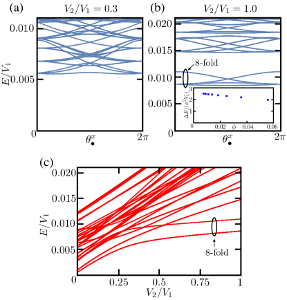
Next, let us consider the many-body states with , which
occupy the same number of sublattices and . Here, we
focus on the state. Figure 2 (a) and (b) shows the
dependence of the many-body spectrum at and
, respectively. In Fig. 2 (a), the ground state mixes
with
higher states with the change in boundary conditions, and the ground state
multiplet is not well-defined. On the other hand, in Fig. 2
(b), eight low-energy states are entangled and do not mix with excited states.
In Fig. 2 (c), the many-body spectrum with
for and is plotted as a function
of .
Figure 2: (Color online) Many-body spectrum with at
as a function of (a, b) the twist
and (c) the ratio of the interaction .
(a, b) The remaining parameters are fixed at . The inset in (b) shows the scaled energy gaps as a
function of the magnetic flux .
The behavior of the ground state in the spectral flow changes at
.
Note that the eight-fold ground state multiplet is always gapped for as long as (For , the energy gap of the
eight-fold
ground state multiplet vanishes, and the two decoupled states
should be the ground states). In the inset of the Fig. 2 (b),
the energy gaps at with periodic boundary
conditions are plotted as a function of the magnetic flux , where
is the -th eigenvalue of with .
The result indicates that the scaling low is roughly
valid in the wide range of . Since the electron density is obtained as
, we have ,
which means that the excitations are local.
Following the argument of the Ref. \citenPhysRevB.95.125134, the obtained
Chern number matrix suggests the -matrix as , where is the degeneracy.
The matrices defined by the eight-fold ground state at are
numerically observed as
(18)
As for a conventional bilayer FQH system with finite
interlayer separation , the pseudopotential does not have the SU(2) symmetry
arising from the pseudospin. However, in the limit or
, the system is exceptionally SU(2) invariant. Therefore, the ground
states of the case in these two limits are described by the
composite
fermion Fermi sea. The former is the two decoupled states and the latter is the
pseudospin-singlet state.
[54]
On the other hand, the Halperin 331 state, which does not have the SU(2)
symmetry, is realized as the ground state in the intermediate separation.
[18, 19, 20]
The FQH system for the LL of graphene in the continuum limit
corresponds to the conventional bilayer FQH system with , where the
Halperin 331 state should not be observed because there is SU(2) symmetry
in the system.
In contrast, the NN and NNN interactions in
the honeycomb lattice act between the different and same sublattices
(chiralities).
Therefore, by connecting the parameter and with the interlayer
and intralayer interactions, the FQH system of the Landau band
corresponds to the conventional bilayer quantum Hall system
with ; the
chirality plays the role of the two-layer index. Note that the only
-component of the pseudospin is conserved in both systems.
Thus, it is natural to expect that the analogue of the Halperin
331 state is realized for the Landau band when the ratio is on
the order of unity. We confirmed this scenario for the four-electron system
in terms of the Chern number matrix as Eq. (18).
The chirality-unpolarized ground state at is also considered in terms
of the Chern number matrix. In the conventional bilayer system at ,
for example, the Halperin 551 state is one of the candidates of the gapped
ground state[18, 54].
However, the results at are not systematic, and no clear picture is
obtained in contrast to the case. They will be discussed later
elsewhere.
To summarize, we have constructed the Chern number matrix in association with
the chiral basis by using the Hamiltonian projected into the
Landau band of the honeycomb lattice. Modifying the interaction range induces
the quantum phase transitions associated with the chirality ferromagnetism.
When the NN interactions are sufficiently strong, the ground
states at and are chirality-polarized, and consistent with the
Laughlin state and the composite fermion Fermi sea, respectively. On the
other hand, an increase in the strength of the NNN interaction
leads the ground state to chirality-unpolarize. The obtained Chern
number matrix indicates that the unpolarized ground state for large at
is consistent with the Halperin 331 state.
Acknowledgements.
This work is partly supported by Grants-in-Aid for Scientific Research,
(KAKENHI), Grant numbers 17H06138, 16K13845, and 25107005.
References
[1]
X. G. Wen: Phys. Rev. B 40 (1989) 7387.
[2]
Y. Hatsugai: Journal of the Physical Society of Japan 73 (2004)
2604.
[3]
Y. Hatsugai: Journal of the Physical Society of Japan 74 (2005)
1374.
[4]
K. v. Klitzing, G. Dorda, and M. Pepper: Phys. Rev. Lett. 45 (1980)
494.
[5]
D. C. Tsui, H. L. Stormer, and A. C. Gossard: Phys. Rev. Lett. 48
(1982) 1559.
[6]
D. J. Thouless, M. Kohmoto, M. P. Nightingale, and M. den Nijs: Phys. Rev.
Lett. 49 (1982) 405.
[7]
Q. Niu, D. J. Thouless, and Y.-S. Wu: Phys. Rev. B 31 (1985) 3372.
[8]
M. Kohmoto: Annals of Physics 160 (1985) 343 .
[9]
M. V. Berry: Proceedings of the Royal Society of London. A. Mathematical and
Physical Sciences 392 (1984) 45.
[10]
R. B. Laughlin: Phys. Rev. Lett. 50 (1983) 1395.
[11]
D. Arovas, J. R. Schrieffer, and F. Wilczek: Phys. Rev. Lett. 53
(1984) 722.
[12]
J. K. Jain: Phys. Rev. Lett. 63 (1989) 199.
[13]
B. I. Halperin, P. A. Lee, and N. Read: Phys. Rev. B 47 (1993)
7312.
[14]
R. Willett, J. P. Eisenstein, H. L. Störmer, D. C. Tsui, A. C. Gossard, and
J. H. English: Phys. Rev. Lett. 59 (1987) 1776.
[15]
G. Moore and N. Read: Nuclear Physics B 360 (1991) 362.
[16]
N. Read and E. Rezayi: Phys. Rev. B 54 (1996) 16864.
[17]
B. I. Halperin: Helv. Phys. Acta 56 (1983) 75.
[18]
D. Yoshioka, A. H. MacDonald, and S. M. Girvin: Phys. Rev. B 39
(1989) 1932.
[19]
S. He, S. Das Sarma, and X. C. Xie: Phys. Rev. B 47 (1993) 4394.
[20]
J. P. Eisenstein, G. S. Boebinger, L. N. Pfeiffer, K. W. West, and S. He: Phys.
Rev. Lett. 68 (1992) 1383.
[21]
K. Nomura and D. Yoshioka: Journal of the Physical Society of Japan 73 (2004) 2612.
[22]
M. R. Peterson and S. Das Sarma: Phys. Rev. B 81 (2010) 165304.
[23]
Z. Papić, M. O. Goerbig, N. Regnault, and
M. V. Milovanović: Phys. Rev. B 82 (2010) 075302.
[24]
X. G. Wen and A. Zee: Phys. Rev. B 46 (1992) 2290.
[25]
X. G. Wen and A. Zee: Phys. Rev. Lett. 69 (1992) 953.
[26]
B. Blok and X. G. Wen: Phys. Rev. B 42 (1990) 8133.
[27]
B. Blok and X. G. Wen: Phys. Rev. B 43 (1991) 8337.
[28]
D. N. Sheng, L. Balents, and Z. Wang: Phys. Rev. Lett. 91 (2003)
116802.
[29]
T.-S. Zeng, W. Zhu, and D. N. Sheng: Phys. Rev. B 95 (2017) 125134.
[30]
X. Du, I. Skachko, F. Duerr, A. Luican, and E. Y. Andrei: Nature 462 (2009) 192 EP .
[31]
K. I. Bolotin, F. Ghahari, M. D. Shulman, H. L. Stormer, and P. Kim: Nature
462 (2009) 196 EP .
[32]
C. R. Dean, A. F. Young, P. Cadden-Zimansky, L. Wang, H. Ren, K. Watanabe,
T. Taniguchi, P. Kim, J. Hone, and K. L. Shepard: Nature Physics 7 (2011) 693 EP .
[33]
F. Ghahari, Y. Zhao, P. Cadden-Zimansky, K. Bolotin, and P. Kim: Phys. Rev.
Lett. 106 (2011) 046801.
[34]
B. E. Feldman, B. Krauss, J. H. Smet, and A. Yacoby: Science 337
(2012) 1196.
[35]
K. Nomura and A. H. MacDonald: Phys. Rev. Lett. 96 (2006) 256602.
[36]
V. M. Apalkov and T. Chakraborty: Phys. Rev. Lett. 97 (2006)
126801.
[37]
C. Tőke, P. E. Lammert, V. H. Crespi, and
J. K. Jain: Phys. Rev. B 74 (2006) 235417.
[38]
C. Tőke and J. K. Jain: Phys. Rev. B
75 (2007) 245440.
[39]
N. Shibata and K. Nomura: Phys. Rev. B 77 (2008) 235426.
[40]
Z. Papić, M. Goerbig, and N. Regnault: Solid State Communications 149 (2009) 1056 .
[41]
N. Shibata and K. Nomura: Journal of the Physical Society of Japan 78 (2009) 104708.
[42]
Z. Papić, M. O. Goerbig, and N. Regnault:
Phys. Rev. Lett. 105 (2010) 176802.
[43]
Z. Papić, R. Thomale, and D. A. Abanin: Phys.
Rev. Lett. 107 (2011) 176602.
[44]
D. A. Abanin, B. E. Feldman, A. Yacoby, and B. I. Halperin: Phys. Rev. B
88 (2013) 115407.
[45]
A. C. Balram, C. Tőke, A. Wójs, and J. K.
Jain: Phys. Rev. B 92 (2015) 075410.
[46]
F. D. M. Haldane: Phys. Rev. Lett. 51 (1983) 605.
[47]
Y. Hamamoto, H. Aoki, and Y. Hatsugai: Phys. Rev. B 86 (2012)
205424.
[48]
Y. Hamamoto, T. Kawarabayashi, H. Aoki, and Y. Hatsugai: Phys. Rev. B
88 (2013) 195141.
[49]
Y. Hatsugai, T. Morimoto, T. Kawarabayashi, Y. Hamamoto, and H. Aoki: New
Journal of Physics 15 (2013) 035023.
[50]
Y. Hatsugai, K. Ishibashi, and Y. Morita: Phys. Rev. Lett. 83
(1999) 2246.
[51]
K. Kudo, T. Kariyado, and Y. Hatsugai: Journal of the Physical Society of Japan
86 (2017) 103701.
[52]
F. D. M. Haldane: Phys. Rev. Lett. 55 (1985) 2095.
[53]
T. Fukui, Y. Hatsugai, and H. Suzuki: Journal of the Physical Society of Japan
74 (2005) 1674.
[54]
V. W. Scarola and J. K. Jain: Phys. Rev. B 64 (2001) 085313.