An Empirical Study of Fault Localization Families and Their Combinations

Abstract

The performance of fault localization techniques is critical to their adoption in practice. This paper reports on an empirical study of a wide range of fault localization techniques on real-world faults. Different from previous studies, this paper (1) considers a wide range of techniques from different families, (2) combines different techniques, and (3) considers the execution time of different techniques. Our results reveal that a combined technique significantly outperforms any individual technique (200% increase in faults localized in Top 1), suggesting that combination may be a desirable way to apply fault localization techniques and that future techniques should also be evaluated in the combined setting. Our implementation is publicly available for evaluating and combining fault localization techniques.

1 Introduction

The goal of fault localization is to identify defective program elements related to software failures. Automated fault localization uses static and run-time information about the program to identify program elements that may be the root cause of the failure. This paper considers seven families of fault localization techniques, which take as input seven different types of information:

• Spectrum-based fault localization (SBFL) [1, 2, 3]: utilizing test coverage information

• Mutation-based fault localization (MBFL) [4, 5]: utilizing test results from mutating the program

• Dynamic program slicing [6, 7]: utilizing dynamic program dependencies

• Stack trace analysis [8, 9]: utilizing crash reports

• Predicate switching [10]: utilizing test results from mutating the results of conditional expressions

• Information-retrieval-based fault localization (IR-based FL) [11]: utilizing bug report information

• History-based fault localization [12, 13]: utilizing the development history

Some techniques compute a suspiciousness score for each program element and can generate a ranked list of elements, such as spectrum-based fault localization. Other techniques only mark a set of elements as suspicious, such as dynamic program slicing.

The performance of fault localization is critical to its adoption in practice. Fault localization techniques are helpful only when the root causes are ranked at a high absolute position [14, 15], such as within the top 5 [16]. A number of empirical studies [17, 18, 19, 20] have evaluated the performance of SBFL and MBFL. However, no empirical study has evaluated the performance of other techniques on real-world faults, as far as we know.

This paper reports on an empirical study of a wide range of fault localization techniques from different families. Following the insight from existing work [17] that the performance of fault localization techniques may differ between real faults and artificial faults, our study is based on 357 real-world faults from the Defects4J dataset [21].

Our study has two main novel aspects. First, since techniques in different families use different information sources, it is interesting to know how much these techniques are correlated to each other. We measured the correlation between different pairs of techniques and explored the possibility of combining these techniques using the learning to rank model [22]. In contrast, previous work usually considers techniques in one or a few families [23], e.g., combining different formulae in SBFL [24] or combining SBFL and history-based techniques [25], and our work, CombineFL, is the first to explore combinations of a wide range of techniques that rely on different information sources.

The second novelty is that we measured the time cost of different fault localization techniques. Existing studies have shown that efficiency and scalability are both critical to the adoption of fault localization techniques [16]. Thus, a good fault localization approach must balance between localization performance and cost. We have considered different usage scenarios to find the best balance in practice.

We also improved the measurement of fault localization performance by designing a new measurement $E_{\mathit{inspect}}$ that calculates the expected rank when multiple faulty elements are presented in ties.

Finally, we have released our experimental infrastructure CombineFL-core and the fault localization data of the studied techniques, which can be used by other researchers to evaluate fault localization techniques and to combine different fault localization techniques.

Our study has the following main findings:

• On real-world faults, all techniques except for Bugspots and BugLocator localize more than 6% of faults in the top 10. The best family, SBFL, localizes about 44% faults of in the top 10.

• Most techniques in our study are weakly correlated with each another, especially those in different families, indicating the potential of combining them.

• CombineFL improves performance significantly: 200/63/51/31% increase in localized faults in the top 1/3/5/10, compared to the best standalone technique.

• CombineFL also outperforms the four state-of-the-art fault localization approaches, MULTRIC [24], Savant [26], FLUCCS [25], and TraPT [27] by 133%, 167%, 11% and 18% in Top 1 correspondingly.

• Time costs of different fault localization families can be categorized into several levels. When using a technique at one time cost level, it does not affect run time to include all techniques from the preceding levels, but it does improve fault localization effectiveness.

• The above findings hold at both statement and method granularities — that is, when the FL technique is identifying suspicious statements and when it is identifying suspicious methods.

To sum up, the paper makes the following contributions.

• The first empirical study that compares a wide range of fault localization techniques on real faults.

• A combined technique, CombineFL, which is configurable based on the time cost, and the peak performance of the technique significantly outperforms standalone techniques.

• An infrastructure, CombineFL-core, for evaluating and combining fault localization techniques for future research.

The rest of the paper is organized as follows. Section 2 presents background about several fault localization families. Section 3 gives the empirical evaluation methodology. Section 4 shows the experiment results and answers the research questions. Section 5 discusses related research. Section 6 discusses the implications for future research. Section 7 concludes.

2 Background

Commonly, a fault localization technique takes as input a faulty program and a set of test cases with at least one failed test, and it generates as output a potentially ranked list of suspicious program elements. Recently, some approaches [11, 28, 13] considered other input information, such as the bug report or the development history. This paper also considers these approaches. The common levels of granularity for program elements are statements, methods, and files. This paper uses statements as program elements, except for Sections 4.5 and 4.6 which compare results for different granularities.

This section first introduces seven families of fault localization techniques, and then introduces the learning to rank model for combining different techniques.

2.1 Spectrum-Based Fault Localization

A program spectrum is a measurement of run-time behavior, such as code coverage [3]. Collofello and Cousins proposed that program spectra be used for fault localization [29]. Comparing program spectra on passed and failed test cases enable ranking of program elements. The more frequently an element is executed in failed tests, and the less frequently it is executed in passed tests, the more suspicious the element is.

Typically, an SBFL approach calculates suspiciousness scores using a ranking metric [30, 31, 32], or risk evaluation formula [1, 33], based on four values collected from the executions of the tests, as shown in Table I. For example, Ochiai [2] and DStar [34] are effective SBFL techniques [33, 35, 17] using the formulas:

$$\mathit{Ochiai}(\mathit{element}) = \frac{e_{f}}{\sqrt{(e_{f}+n_{f})\cdot(e_{f}+e_{p})}}$$

$$\mathit{DStar}(\mathit{element}) = \frac{e_{f}^{*}}{e_{p}+n_{f}}$$

DStar’s notation ‘*’ is a variable, which we set to 2 based on the recommendation from Wong et al. [34].

TABLE I: Input Values for Spectrum-Based Fault Localization

$e_{f}$	Number of failed tests that execute the program element.
$e_{p}$	Number of passed tests that execute the program element.
$n_{f}$	Number of failed tests that do not execute the program element.
$n_{p}$	Number of passed tests that do not execute the program element.

2.2 Mutation-Based Fault Localization

Mutation-based fault localization uses information from mutation analysis [36], rather than from regular program execution, as inputs to its ranking metric or risk evaluation formula. While SBFL techniques consider whether a statement is executed or not, MBFL techniques consider whether the execution of a statement affects the result of a test by injecting mutants. A mutant typically changes one expression or statement by replacing one operand or expression with another [17]. If a program statement affects failed tests more frequently and affects passed tests more rarely, it is more suspicious.

For a statement $s$, a MBFL technique:

• generates a set of mutants $m(s)=\langle m_{1}(s),m_{2}(s),...\rangle$,

• assigns each mutant a score $S_{\mathit{mutant}}(m_{i}(s))$, and

• aggregates the scores to a statement suspiciousness score $S_{\mathit{statement}}(s)$.

MUSE [5] and Metallaxis-FL [4] are two state-of-the-art MBFL techniques.

MUSE assigns each mutant a suspiciousness score as follows:

$$S_{\mathit{mutant}}(m_{i})=\mathit{failed}(m_{i})-\frac{f2p}{p2f}\cdot\mathit{passed}(m_{i})$$

where $\mathit{failed}(m_{i})$ is the number of test cases that failed on the original program but now pass on a mutant $m_{i}$, and likewise for $\mathit{passed}(m_{i})$. $f2p$ is the number of test cases that change from fail to pass on any mutant, and likewise for $p2f$. To aggregate mutant suspiciousness scores into a statement suspiciousness score, MUSE uses $S_{\mathit{statement}}(s)=Avg_{m_{i}\in m(s)}S_{\mathit{mutant}}(m_{i})$.

Metallaxis assigns each mutant a suspiciousness score using the Ochiai formula:

$$S_{\mathit{mutant}}(m_{i})=\frac{\mathit{failed}(m_{i})}{\sqrt{\mathit{totalfailed}\cdot(\mathit{failed}(m_{i})+\mathit{passed}(m_{i}))}}$$

where $\mathit{failed}(m_{i})$ is the number of test cases that failed on the original program and now the output changes on a mutant $m_{i}$, and similarly for $\mathit{passed}(m_{i})$. $\mathit{totalfailed}$ is the total number of test cases that fail on the original program.

A mutant is said to be killed by a test case if the test case has different execution results on the mutated program and the original program [37]. A test case that kills mutants may carry diagnostic information. Note that the definition of killed in MUSE and Metallaxis is different. In MUSE, a failed test case must change to passed to count as killing a mutant. In Metallaxis, a failed test case only needs to generate a different output (may still be failed) to count as killing a mutant.

2.3 Program Slicing

A slicing criterion is a set of variables at a program location; for example, they might be variables that have unexpected or undesired values. A program slice is a subset of program elements that potentially affect the slicing criterion [38].

Program slicing was introduced as a debugging tool to reduce a program to a minimal form while still maintaining a given behavior [39]. Static slicing only uses the source code and accounts for all possible executions of the program.

Dynamic slicing focuses on one execution for a specific input [40]. The key difference between dynamic slicing and static slicing is that dynamic slicing only includes executed statements for the specific input, but static slicing includes possibly-executed statements for all potential inputs. Since dynamic slices are significantly smaller, they are more suitable and effective for program debugging [41].

The following example shows the difference between static slicing and dynamic slicing.

⬇

int collatz(int x) {

1: int res;

2: if ((x % 2) == 0)

3: res = x / 2;

4: else

5: res = x * 3 + 1;

6: return res;

}

The collatz function returns $x/2$ when $x$ is even and returns $3x+1$ when $x$ is odd. Let the slicing criterion be res at line 6. Static slicing includes statements in both the then and else block, because both may affect the value of res. Dynamic slicing considers a particular execution of the program. For example, for x=3, the dynamic slice would contain line 5, but would not contain line 3.

2.4 Stack trace Analysis

A stack trace is the list of active stack frames during execution of a program. Each stack frame corresponds to a function call that has not yet returned. Stack traces are useful information sources for developers during debugging tasks. When the system crashes, the stack trace indicates the currently active function calls and the point where the crash occurred.

2.5 Predicate Switching

Predicate switching [10] is a fault localization technique designed for faults related to control flow. A predicate, or conditional expression, controls the execution of different branches. If a failed test case can be changed to a passed test case by modifying the evaluated result of a predicate, the predicate is called a critical predicate and may be the root cause of the fault.

The technique first traces the execution of the failed test and identifies all instances of branch predicates. Then it repeatedly re-runs the test, forcibly switching the outcome of a different predicate each time. If switching a predicate produces the correct output, the predicate is potentially the cause of the fault and is called a critical predicate.

Predicate switching is similar to MBFL techniques, as they both apply mutations and examine the change of the execution results. We treat predicate switching as a different family because predicate switching mutates the control flow rather than the program itself. For example, if a conditional expression has been evaluated multiple times during the program execution, predicate switching inverses one evaluation at a time instead of all evaluations. Furthermore, previous work [17, 27] does not include predicate switching as an MBFL approach as far as we are aware.

2.6 Information Retrieval-Based Fault Localization

Information Retrieval (IR) was initially used to index text and search for documents [42]. Recent studies [11, 43, 28, 44] have applied information retrieval techniques to fault localization. These approaches take as input a bug report, rather than a set of test cases, and generate as output a list of relevant source code files [45].

These approaches treat the bug reports as a query and then rank the source code files by their relevance to the query. Unlike aforementioned fault localization families, IR-based fault localization techniques do not require program execution information, such as passed and failed test cases. They locate relevant files based on the bug report [11].

2.7 History-Based Fault Localization

Program files that contained more bugs in the past are likely to have more bugs in the future [46]. Development history can be used for fault prediction, which ranks the elements in a program by their likelihood to be defective. Traditionally, fault prediction and fault localization are considered as different problems, and fault prediction runs before any failure has been discovered [12]. However, since they both produce a list of suspicious elements, this paper also considers fault prediction techniques.

We consider a simple fault prediction technique introduced by Rahman et al. [13]. This technique ranks files by the number of fixing changes applied on them. This simple technique has the same utility for inspections as a more sophisticated fault prediction technique, FixCache [12].

2.8 Learning to Rank

Learning to rank techniques train a machine learning model for a ranking task [47]. Learning to rank is widely used in Information Retrieval (IR) and Natural Language Processing (NLP) [48]. For example, in document retrieval, the task is to sort documents by their relevance to a query. One way to create the ranking model is with expert knowledge. By contrast, learning to rank techniques improve ranking performance and automatically create the ranking model, integrating many features (or signals).

Liu categorized learning to rank models into three groups [48]. Pointwise techniques transform the rank problem into a regression or ordinal classification problem for the ordinal score in the training data. Pairwise techniques approximate the problem by a classification problem: creating a classifier for classifying item pairs according to their ordinal position. The goal of pairwise techniques is to minimize ordinal inversions. Listwise techniques take ranking lists as input and evaluate the ranking lists directly by the loss functions.

Recently, Xuan and Monperrus showed that learning to rank model can be used to combine different formulae in SBFL [24]. The basic idea is to treat the suspiciousness score produced by different formulae as features and use learning to rank to find a model that ranks the faulty element as high as possible. In this paper we apply learning to rank similarly to combine techniques from different families.

3 Experimental Methodology

3.1 Experiment Overview and Research Questions

Our experiments investigate the following research questions.

RQ1:  How effective are the standalone fault localization techniques?

This question helps us to understand the performance of widely-used techniques.

RQ2:  Are these techniques correlated? What is their correlation?

This question explores the possibility of combining different techniques. If different techniques are not correlated, then combining them may archive better performance.

RQ3:  How effectively can we combine these techniques using learning to rank?

This question considers a specific way of combining different techniques, and evaluates the performance of the combined technique.

RQ4:  What is the run-time cost of standalone techniques and combined techniques?

The previous question only concerns the effectiveness of the combined techniques. This question considers the efficiency. The best technique for a given use case balances effectiveness and efficiency.

RQ5:  Are the results the same for statement and method granularity?

We shall answer the preceding four questions first at statement granularity, which is often used in evaluating fault localization approaches [49, 33, 50, 51] and in downstream applications such as program repair [52, 53, 54]. On the other hand, several studies have suggested that methods may be a better granularity for developers [26, 55], so we repeated the experiments for the above questions at the method granularity.

RQ6:  How effective the combined approach is when compared with the state-of-the-art techniques?

Recently, a set of new fault localization approaches were proposed. Interestingly, they also use learning to rank to combine existing techniques or other features. This research question compares the performance of our combined approach to these approaches.

3.2 Experimental Subjects

Our experiments evaluate fault localization techniques on the Defects4J [21] benchmark, version v1.0.1 (Footnote 2). Defects4J contains 357 faults minimized from real-world faults in five open-source Java projects. Many previous studies on fault localization used Defects4J as their benchmarks [56, 26, 17]. For each fault, Defects4J provides a faulty version of the project, a fixed version of the project, and a suite of test cases that contains at least one failed test case that triggers the fault.

TABLE II: Defects4J Dataset (version 1.0.1). ‘Faults’ is the number of defective versions of the program. ‘LoC’ is average lines of code for each buggy version of the project, as reported by cloc.

Project	Faults	LoC
Apache Commons Math	106	103.9k
Apache Commons Lang	65	49.9k
Joda-Time	27	105.2k
JFreeChart	26	132.2k
Google Closure compiler	133	216.2k
Total	357	138.0k

3.3 Studied Techniques and Their Implementations

A fault localization technique outputs one of the following:

• A ranked list. Examples include the SBFL, MBFL, stack trace, and history-based families, and one slicing technique.

• A suspicious set. The techniques do not distinguish the suspiciousness between these elements. Examples include the predicate switching family and some slicing techniques.

3.3.1 SBFL and MBFL

Pearson et al. [17] studied the performance of SBFL and MBFL on Defects4j, and our experiments reuse their infrastructure and the collected test coverage information. For SBFL, we used only the two techniques that performed best in Pearson et al.’s study: Ochiai [2] and DStar [34]. The parameter $*$ in DStar is set to $2$. For MBFL, we used the two mainstream MBFL techniques, MUSE [5] and Metallaxis [4]. The formulae for calculating the suspiciousness are introduced in Sections 2.1 and 2.2.

3.3.2 Dynamic Slicing

The JavaSlicer dynamic slicing tool [57] is based on the dynamic slicing algorithm of Wang and Roychoudhury [58, 59], with extensions for object-oriented programs. The JavaSlicer implementation attaches to the program as a Java agent and rewrites classes as they are loaded into the Java VM.

A test fails by throwing an exception, either because of a violated assertion or a run-time crash. If there is only a single failed test, we use the execution of the statement that throws the exception as the slicing criterion. The slice then contains all statements that may have affected the statement that throws the exception.

If there are multiple failed tests, our experiments apply three strategies from a previous study [60] to utilize multiple slices: union, intersection, and frequency. The first two strategies calculate the union or the intersection of the slices and report a set of statements as results. The frequency strategy calculates the inclusion frequency for each statement and reports a ranked list of statements based on the frequency. The more frequently a statement is included in the slice of a failed test, the more suspicious the statement is.

3.3.3 Stack Trace Analysis

According to Schroter et al. [61], if the stack trace includes the faulty method around 40% of the faults can be located in the very first frame, and 90% of the faults can be located within the top 10 stack frames.

We defined a stack trace technique based on this insight. If the exception is thrown by the testing framework (such as JUnit), then the technique returns an empty suspicious list. Otherwise, we call the fault a crash fault and the suspicious list consists of the frames in the stack trace. The frame at depth $d$ is given suspiciousness score $1/d$ score. The score of an element (method) is its maximum score in all failed tests.

3.3.4 Predicate Switching

We re-implemented Zhang et al.’s method of predicate switching for Java (the original implementation was for x86/x64 Linux binaries) [10]. Our implementation of the technique is based on Eclipse Java development tools (JDT). The technique first traces the execution of the failed test case and records all executed predicates. Then it forcibly switches the outcome of a predicate at run time. Once switching a predicate makes the failed test case pass, it reports the predicate as a critical predicate. The technique produces a set of critical predicates as the suspicious program elements.

3.3.5 IR-based Fault Localization

BugLocator [11] ranks all files based on the textual similarity between the initial bug report and the source code file using a revised Vector Space Model (rSVM).

Since the granularity in BugLocator is source file, our implementation uses the file score for all statements in it. For example, if BugLocator reports that file1.java has suspiciousness score 0.2, then it marks every executable statement in file1.java with suspiciousness score 0.2.

3.3.6 History-Based Fault Localization

Bugspots is an implementation of Rahman et al.’s algorithm [13]. Bugspots collects revision control changes with descriptions related to ‘fix’ or ‘close’. The tool ranks more recent bug-fixing changes higher than older ones.

the granularity in Bugspots is source file. Our implementation maps the score of a suspicious file to all executable statements as in Section 3.3.5.

Bugspots supports only Git repositories. However, the version control system of Chart in Defects4J uses a private format of Subversion and neither git-svn nor svn2git can convert this format. As a result, our experiments apply Bugspots on the Math, Lang, Time, and Closure projects.

3.3.7 Learning to Rank

For the learning to rank model, our experiments associate each program statement with a vector

$$\mathit{Suspiciousness}(e)=\langle s_{t_{1}}(e),s_{t_{2}}(e),...\rangle$$

where $e$ is a program element, and $s_{t_{i}}(e)$ is the suspiciousness score of $e$ reported by technique $t_{i}$. The vector values are normalized to be within the domain [0, 1], where 1 is most suspicious and 0 is least suspicious.

Then our experiments apply rankSVM [62] to train the learning to rank model. RankSVM is an open-source learning to rank tool based on LIBSVM [63]. It implements a pairwise learning to rank model and has been used in previous fault localization work [26, 25]. It generates pairwise constraints, e.g., $e^{\mathit{faulty}}_{i}>e^{\mathit{correct}}_{j}$, and the training goal is to rank the faulty elements at the top, i.e., maximize satisfied pairwise constraints.

3.4 Measurements

To evaluate fault localization techniques, we need to measure their performance quantitatively. Previous studies use similar metrics for this measurement, but they may differ in how they handle cases such as insertion or multiple faulty elements. This section describes the measurement methods used in our study.

3.4.1 Determining Faulty Elements

To understand how faulty elements are ranked, we need first to determine which elements in the program are faulty. Following common practice [25, 26, 17], we define the faulty program elements as those modified or deleted in the developer patch that fixes the defect. In the following example patch, i.e., the diff between the fixed and the faulty program, the second line is considered faulty.

⬇

1 if (real == 0.0 && imaginary == 0.0) {

2- return NaN;

3+ return INF;

4 }

5

6 if (isInfinite) {

7 return ZERO;

8 }

9 ...

However, sometimes a developer patch only inserts new elements rather than modifies or deletes old elements. To deal with insertions, we follow the principle used by Pearson et al. [17]: a fault localization technique should report the element immediately following the inserted element. The rationale is that the immediately following element indicates the location that a developer should change to fix the defect.

3.4.2 Multiple Faulty Elements

Many defective programs have multiple defective elements.

In Defects4J, there are two common reasons for multiple faulty elements.

• To repair a fault, the programmer changed multiple elements.

• The patch of a fault not only repairs the current fault but also repairs cloned bugs, i.e., the same bug in cloned code snippets.

Following existing work [17], we consider a fault to be localized by a fault localization technique if any faulty element is localized. It is assumed that if a fault localization technique gives any of the faulty elements, the developer can deduce the other faulty elements. Furthermore, when multiple cloned bugs exist, the developer can re-run fault localization to find the others or can use techniques for repairing cloned bugs [64, 65] to discover and fix other bugs.

3.4.3 Elements with the Same Score

Fault localization techniques often assign the same suspiciousness score to elements, either because the techniques are designed to only locate elements but not to rank them (e.g., union strategy in slicing), or because the techniques cannot distinguish some elements (e.g., statements in a basic block in SBFL). When presenting the suspicious list to the user, the elements with the same score are presented in an arbitrary order, and thus we need to consider the order when measuring the performance.

Previous studies [17, 45, 66] treat elements with the same score as all the $n$th element in the list, where $n$ is their average rank. However, this method may unnecessarily lower their ranks when multiple faulty elements exist. For example, suppose a set of tied elements are all faulty. Then regardless how this set is sorted, the user will find a faulty element at the first element in the set, rather than at the average rank.

To overcome this problem, in our study we measure the performance of a fault localization by the expected rank of the first faulty element, assuming tied elements are arbitrarily sorted. More concretely, assuming a group of $t$ tied elements starting at $P_{start}$ that contains $t_{f}$ faulty elements and there is no faulty element before $P_{\mathit{start}}$, we define ${E_{\mathit{inspect}}}$, which measures the expected rank of the first faulty element using the following formula.

$$E_{\mathit{inspect}}=P_{start}+\sum^{t-t_{f}}_{k=1}k\frac{\binom{t-k-1}{t_{f}-1}}{\binom{t}{t_{f}}}$$

The equation within the summation is the probability for the top-ranked faulty element to appear in the $k$th location after $P_{\mathit{start}}$: that is, the number of all combinations where the first faulty element is at $k$ ($\binom{t-k-1}{t_{f}-1}$) divided by the number of all combinations ($\binom{t}{t_{f}}$).

Notice that, when there is only one faulty element, i.e., $t_{f}=1$, the equation reduces to:

$$E_{\mathit{inspect}}=P_{start}+\frac{t-1}{2}$$

which is the same as average rank, also average accuracy, in existing studies [26, 27].

Also, when all tied elements are faulty, i.e., $t_{f}=t$, the equation reduces to:

$$E_{\mathit{inspect}}=P_{start}$$

which indicates the first element in the tied set.

3.4.4 Metrics

So far we have defined how to calculate the expected rank of the first faulty element. Based on this definition we use two metrics to measure the performance of a fault localization technique.

$\mathbf{E_{\mathit{inspect}}@n}$ counts the number of the 357 faults that were successfully localized within the top $n$ positions of the resultant ranked lists, i.e., the number of faults that $E_{\mathit{inspect}}$ values on these faults are less than or equal to $n$. It is adapted from metric $acc@n$ [26, 27]. A previous study [14] suggested that programmers will only inspect the top few positions in a ranked list, and $E_{\mathit{inspect}}@n$ reflects this.

EXAM [67] is the percentage of elements that have to be inspected until finding a faulty element, averaged across all 357 faults uniformly. It is a commonly used metric for fault localization techniques [17, 30, 68]. The EXAM score measures the relative position of the faulty element in the ranked list. Smaller EXAM scores are better.

The ${E_{\mathit{inspect}}@n}$ metric is a more meaningful measure of fault localization quality than the EXAM score. A developer will only examine the first few reports from a tool (say, 5 or 10) and a program repair tool will only examine the first 200 or so reports. Therefore, any reports other than these are irrelevant and can be disregarded, yet they are most of the reports and dominate the EXAM score. This paper includes the EXAM score to enable comparison with earlier papers.

4 Experiment Results

Our experiments investigate and answer six research questions. The granularity of all experiments is statements, except in Sections 4.5 and 4.6.

4.1 RQ1. Effectiveness of standalone techniques

4.1.1 Procedure

To evaluate the effectiveness of standalone fault localization techniques, we invoked each technique on Defects4J and compared their $E_{\mathit{inspect}}@n$ and EXAM scores. The definitions of $E_{\mathit{inspect}}@n$ and EXAM are in Section 3.4.4.

TABLE III: The Performance of Standalone Techniques on all 357 faults. Boldface indicates the best-performing techniques.

Family	Technique	$E_{\mathit{inspect}}$				EXAM
		@1	@3	@5	@10
SBFL	Ochiai	16 (4%)	81 (23%)	111 (31%)	156 (44%)	0.033
	DStar	17 (5%)	84 (24%)	111 (31%)	155 (43%)	0.033
MBFL	Metallaxis	23 (6%)	78 (22%)	103 (29%)	129 (36%)	0.118
	MUSE	24 (7%)	44 (12%)	58 (16%)	68 (19%)	0.304
slicing	union	5 (1%)	33 (9%)	58 (16%)	84 (24%)	0.207
	intersection	5 (1%)	35 (10%)	55 (15%)	71 (20%)	0.222
	frequency	6 (2%)	39 (11%)	58 (16%)	84 (24%)	0.208
stack trace	stack trace	20 (6%)	31 (9%)	38 (11%)	38 (11%)	0.311
predicate switching	predicate switching	3 (1%)	15 (4%)	20 (6%)	23 (6%)	0.331
IR-based	BugLocator	0 (0%)	0 (0%)	0 (0%)	3 (1%)	0.212
history-based	Bugspots	0 (0%)	0 (0%)	0 (0%)	0 (0%)	0.465

4.1.2 Results and Findings

Table III shows the $E_{\mathit{inspect}}@n$ and EXAM of each standalone technique.

Finding 1.1:  SBFL is the most effective standalone fault localization family in our experiments.

Two techniques of SBFL, Ochiai and DStar, are the best and second best on $E_{\mathit{inspect}}@3,5,10$ and EXAM. The two techniques locate 156 and 155 faults (about 44% of all faults) in the top 10 reports. SBFL may underperform at $E_{\mathit{inspect}}@1$ because blocks are the minimum granularity that SBFL can identify. In a single execution, the statements in a basic block are all executed or not executed, so the elements in a basic block always have the same $\langle e_{f},e_{p},n_{f},n_{p}\rangle$ values and the same score.

Finding 1.2:  Bugspots and BugLocator are not as effective at localizing faulty statements as other techniques.

Bugspots did not locate any fault in its top-10 statements and BugLocator did not locate any fault in its top-5 statements. A possible reason is that the two techniques works at the file granularity and all statements in a file will be tied. Even if the faulty statement is in the identified file, the statement will be tied with many other statements and will not be ranked high.

TABLE IV: The Performance of Techniques on Crash Faults (90 out of 357 faults, 25%)

Family	Technique	$E_{\mathit{inspect}}$				EXAM
		@1	@3	@5	@10
SBFL	Ochiai	4 (4%)	17 (19%)	32 (36%)	50 (56%)	0.028
	DStar	4 (4%)	18 (20%)	33 (37%)	50 (56%)	0.029
MBFL	Metallaxis	10 (11%)	30 (33%)	35 (39%)	44 (49%)	0.083
	MUSE	6 (7%)	13 (14%)	18 (20%)	19 (21%)	0.345
slicing	union	2 (2%)	13 (14%)	26 (29%)	36 (40%)	0.112
	intersection	2 (2%)	13 (14%)	21 (23%)	30 (33%)	0.136
	frequency	2 (2%)	14 (16%)	25 (28%)	36 (40%)	0.112
stack trace	stack trace	20 (22%)	31 (34%)	38 (42%)	38 (42%)	0.194
predicate switching	predicate switching	1 (1%)	5 (6%)	8 (9%)	9 (10%)	0.323
IR-based	BugLocator	0 (0%)	0 (0%)	0 (0%)	0 (0%)	0.199
history-based	Bugspots	0 (0%)	0 (0%)	0 (0%)	0 (0%)	0.433

Finding 1.3:  Stack trace is the most effective technique on crash faults.

Stack trace analysis only works on crash faults (Section 3.3.3). In the Defects4J dataset, 25% of the faults (90 out of 357) are crash faults, including application-defined exceptions, out of memory errors, and stack overflow errors. Table IV shows that stack trace analysis locates 22% of crash faults (20 out of 90) at top-1. By contrast, the second best technique on these crash faults is Metallaxis, which identifies 11% of faults (10 out of 90) at top-1. This finding indicates that the stack trace is a vital information source for crash faults. It is also consistent with debugging scenarios in practice: when a program crashes, the developer often starts by examining the stack trace.

TABLE V: The Performance of Techniques on Predicate-Related Faults (115 out of 357 faults, 32%)

Family	Technique	$E_{\mathit{inspect}}$				EXAM
		@1	@3	@5	@10
SBFL	Ochiai	5 (4%)	20 (17%)	29 (25%)	43 (37%)	0.027
	DStar	5 (4%)	21 (18%)	30 (26%)	43 (37%)	0.028
MBFL	Metallaxis	8 (7%)	25 (22%)	34 (30%)	44 (38%)	0.090
	MUSE	13 (11%)	24 (21%)	32 (28%)	35 (30%)	0.174
slicing	union	0 (0%)	6 (5%)	12 (10%)	26 (23%)	0.171
	intersection	0 (0%)	9 (8%)	13 (11%)	20 (17%)	0.185
	frequency	0 (0%)	10 (9%)	15 (13%)	27 (23%)	0.172
stack trace	stack trace	4 (3%)	7 (6%)	10 (9%)	10 (9%)	0.255
predicate switching	predicate switching	3 (3%)	15 (13%)	20 (17%)	23 (20%)	0.216
IR-based	BugLocator	0 (0%)	0 (0%)	0 (0%)	1 (0%)	0.156
history-based	Bugspots	0 (0%)	0 (0%)	0 (0%)	0 (0%)	0.417

Finding 1.4:  Predicate switching is not the most effective technique on “predicate-related” faults.

A predicate-related fault is one whose patch modifies the predicate in a conditional statement. In the Defects4J dataset, 32% of the faults are predicate-related faults. Table V shows the performance of each standalone technique on predicate-related faults. It was surprising to us that MBFL family works better than predicate switching on predicate-related faults. When working on predicates, MBFL and predicate switching have similar mechanisms. They both modify the predicates and check whether the execution result changes. Predicate switching may underperform MBFL because MBFL can further rank the critical predicates (modifying which can change the execution result) while predicate switching cannot.

4.2 RQ2. Correlation between Techniques

This research question explores the possibility of combining different techniques. Two techniques are (positively) correlated if they are good at localizing the same sorts of faults. If two techniques are less correlated, they may provide different information, and combining them has the potential to outperform either of the component techniques.

4.2.1 Procedure

First, to visually illustrate the correlation between techniques, we drew the results of each pair of techniques as a scatter plot. Each figure has 357 points, one for each fault in our dataset. The coordinate $(x,y)$ for a fault means on this fault, the $E_{\mathit{inspect}}$ for technique on X-axis is $x$, and the $E_{\mathit{inspect}}$ for technique on Y-axis is $y$.

To quantify the correlation between each pair of techniques, we computed coefficient of determination $r^{2}$, which measures of the linear correlation between two variables [69]. Recall that a developer will only examine the first few reports from a tool (say, 5 or 10) and a program repair tool will only examine the first 200 or so reports. When computing the correlation, we used all points such that $x\leq q$ or $y\leq q$, for threshold $q=100$. We also computed the $p$-value, to determine whether the correlation coefficient is statistically significant.

4.2.2 Qualitative Results

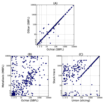
Figure 1: The Correlation of Three Example Pairs of Techniques. The X and Y values for a point show the $E_{\mathit{inspect}}$ values for two techniques on the same bug. $E_{\mathit{inspect}}$ is the expected rank of the first faulty element in the FL tool’s output, or the number of elements that a user would have to inspect before inspecting a faulty element.

Figure 1’s scatter plots visualize the correlation between three sample pairs of techniques. The three pairs capture typical patterns of the plots, and we omit the rest of the plots as they are similar to one of the three plots.

Finding 2.1:  Different correlation patterns exist between different pairs of techniques.

In Fig. 1 (A), most points lie on the diagonal. This distribution pattern means the two SBFL techniques, Ochiai and DStar, have almost the same $E_{\mathit{inspect}}$ values on all faults. The two techniques are very correlated and each is unlikely to provide more information than the other.

In Fig. 1 (B), there are many faults located in upper-left and lower-right regions, which correspond to faults that one technique works well on, while the other works poorly. These faults suggest that the two techniques are not positively correlated.

The dots in Fig. 1 (C) are located on the diagonal in the upper right region, but they are scattered in other regions. This pattern indicates that there are a set of faults where both techniques perform poorly, but there are also many faults where one technique performs well but the other does not.

4.2.3 Quantitative Results

Table VI shows the coefficient of determination, $r^{2}$, between each pair of techniques. Different from Fig. 1, which is a log-scale plot, this experiment calculates $r^{2}$ based on $E_{\mathit{inspect}}$, without log-scale normalization. Notice that the table is a symmetric matrix.

Finding 2.2:  Most techniques are weakly correlated, including all techniques in different families.

In Table VI, there are 55 pairs of different techniques. Only two of them are significantly correlated at $p$-value less than 0.05 level: $\langle$Ochiai, DStar$\rangle$ from SBFL, with $r^{2}=0.753$, $p$-value $\ll 0.01$, and $\langle$union, frequency$\rangle$ from slicing, with $r^{2}=0.310$, $p$-value $\ll 0.01$. The $r^{2}$ values in other pairs of techniques are much smaller, and the $p$-values of them are larger than 0.05, which suggests that there is no statistically significant correlation between other pairs of techniques, at least for the reports that a programmer or tool may view.

Two techniques may provide different information when they are less correlated. Since there exist many weakly correlated pairs, if a method could utilize the information from different techniques, it may improve the effectiveness of fault localization.

Finding 2.3:  The strongly correlated techniques only exist in the same family, but not all techniques in the same family are strongly correlated.

The most correlated pair of techniques, Ochiai and DStar, is from the SBFL family. The second most correlated pair is from the slicing family. However, not all techniques from the same family are strongly correlated. For example, the two from MBFL family are weakly correlated, and so is intersection with other slicing techniques. This finding suggests that though it may be less promising to combine techniques from the same family, it is still worth investigating.

TABLE VI: $r^{2}$ between Pairs of Techniques. The two pairs of statistically significantly correlated techniques ($p$-value $<0.05$) are highlighted.

	Family	SBFL		MBFL		slicing			stack trace	predicate switching	IR-based	history-based
Family	Technique	Ochiai	DStar	Metallaxis	MUSE	union	intersection	frequency	stack trace	predicate switching	BugLocator	Bugspots
SBFL	Ochiai	-	0.753	0.001	0.005	0.000	0.001	0.001	0.000	0.001	0.001	0.000
	DStar	0.753	-	0.001	0.004	0.000	0.000	0.000	0.000	0.001	0.001	0.000
MBFL	Metallaxis	0.001	0.001	1.000	0.002	0.008	0.005	0.005	0.004	0.003	0.003	0.001
	MUSE	0.005	0.004	0.002	1.000	0.012	0.013	0.013	0.015	0.009	0.015	0.024
slicing	union	0.000	0.000	0.008	0.012	-	0.004	0.310	0.009	0.010	0.003	0.000
	intersection	0.001	0.000	0.005	0.013	0.004	-	0.015	0.007	0.009	0.004	0.003
	frequency	0.001	0.000	0.005	0.013	0.310	0.015	-	0.005	0.009	0.003	0.000
stack trace	stack trace	0.000	0.000	0.004	0.015	0.009	0.007	0.005	-	0.014	0.005	0.022
predicate switching	predicate switching	0.001	0.001	0.003	0.009	0.010	0.009	0.009	0.014	-	0.007	0.026
IR-based	BugLocator	0.001	0.001	0.003	0.015	0.003	0.004	0.003	0.005	0.007	-	0.009
history-based	Bugspots	0.000	0.000	0.001	0.024	0.000	0.003	0.000	0.022	0.026	0.009	-

4.3 RQ3. Effectiveness of Combining Techniques

Section 4.2 indicates that the techniques are potentially complementary to each other. This section applies the learning to rank model to combine techniques.

4.3.1 Procedure

Our experiments perform cross-validation to evaluate the ranking model. Cross-validation estimates model performance without losing modeling or test capability despite small data size. In particular, we used two cross-validation methods.

• $k$-fold validation. This simulates within-project training. The original data were randomly split into $k$ different sets of the same size and the training-validation is performed $k$ times, each time training on $k$-1 sets and validating on the other set. We set $k=10$ in our experiment.

• Cross-project validation. This simulates cross-project training. We treat one project as the test set and the other projects as the training sets, and repeat the process for each project.

We performed two sets of experiments to evaluate the combined technique.

• The first experiment measured the performance of combining all techniques.

• The second experiment evaluated the contribution of each fault localization family. We excluded one family at a time and repeated the learning to rank procedure.

TABLE VII: Learning to Rank Results. Comparing cross project validation and $k$-fold validation.

Validation Method	$E_{\mathit{inspect}}$				EXAM
	@1	@3	@5	@10
10-fold	72 (20%)	137 (38%)	168 (47%)	205 (57%)	0.0173
cross project	68 (19%)	130 (36%)	165 (46%)	197 (55%)	0.0171

TABLE VIII: Learning to Rank Results. Learning to rank is significantly better than any original technique. The reduction of excluding a family is marked after the $E_{\mathit{inspect}}$ value. The Ochiai, DStar, and MUSE rows are copied from Table III for comparison.

Family /	$E_{\mathit{inspect}}$				EXAM
Technique	@1	@3	@5	@10
All Families	72 (20%)	137 (38%)	168 (47%)	205 (57%)	0.0173
w/o SBFL	61 (-11)	120 (-17)	145 (-23)	188 (-27)	0.0225
w/o MBFL	52 (-20)	122 (-15)	148 (-20)	194 (-11)	0.0206
w/o slicing	58 (-14)	129 (-8)	165 (-3)	201 (-4)	0.0190
w/o stack trace	63 (-9)	133 (-4)	161 (-7)	199 (-6)	0.0176
w/o predicate  switching	68 (-4)	136 (-1)	165 (-3)	198 (-7)	0.0178
w/o IR-based	66 (-6)	134 (-3)	162 (-6)	194 (-11)	0.0173
w/o history-based	71 (-1)	136 (-1)	167 (-1)	203 (-2)	0.0173
Ochiai	16 (4%)	81(23%)	111 (31%)	156 (44%)	0.033
DStar	17 (5%)	84 (24%)	111 (31%)	155 (43%)	0.033
MUSE	24 (7%)	44 (12%)	58 (16%)	68 (19%)	0.304

4.3.2 Results and Findings

Finding 3.1:  The two cross-validation methods yield similar evaluation results.

Table VII shows the results of the first experiment on validation methods. The evaluation results of the two validation methods are similar. Both of the two validation methods indicate that the combined technique significantly outperforms any standalone techniques in Table III. These results suggest that the learning to rank model we used has good generalizability across different projects. Since the performances of the two methods are close, the rest of the paper reports only 10-fold validation.

Finding 3.2:  The combined technique significantly outperforms any standalone technique.

Table VIII shows the results of the two experiments on combined techniques. The All Families row presents the results of the first experiment, i.e., the results of combining all families. The next rows present the results of the second experiment, where each row shows the performance of excluding one family at a time. The reduction of excluding a family is marked after the $E_{\mathit{inspect}}$ value.

The combined technique in the All families row is significantly better than any standalone techniques. At $E_{\mathit{inspect}}@1,3,5,10$, the combined technique improves 200%, 63%, 46% and 31% over the former best, respectively. At EXAM, it improves from 0.033 to 0.0173, an improvement of 48% from the former best. These results indicate that learning to rank is an effective method to combine different fault localization techniques and the performance of the combined technique is significantly improved.

Finding 3.3:  The contribution of each technique to the combined result is not determined by its effectiveness as a standalone technique.

For example, while the IR-based family could not locate any bugs in Top 1–5 and predicate switching can locate 3–20 bugs in Top 1–5, removing the IR-based family has a larger impact than predicate switching in Top 1–5. This finding indicates that, when considering a fault localization technique, it is not enough to evaluate its individual performance: we need to evaluate it in combination with other techniques.

Finding 3.4:  All families contribute to the overall results.

Table VIII shows that removing any family decreases all metrics. Bugspots, which does not rank any faulty element into the top 10 when used alone, slightly improved all $E_{inspect}@n$ values when combined with other techniques.

TABLE IX: Time Consumption of Each Technique (in seconds, to 2 digits of precision)

Time Level	Family	Technique	Average	Math	Lang	Time	Chart	Closure
Level 1 (Seconds)	history-based	Bugspots	0.54	0.66	0.22	0.20	-	0.67
	stack trace	stack trace	1.3	0.17	0.15	0.39	0.18	3.1
	IR-based	BugLocator	5.6	6.6	4.3	4.7	4.6	5.8
Level 2 (Minutes)	slicing	union	80	44	39	29	47	150
		intersection	80	44	39	29	47	150
		frequency	80	44	39	29	47	150
	SBFL	Ochiai	200	86	26	85	44	430
		DStar	200	86	26	85	44	430
Level 3 (Around ten minutes)	predicate switching	predicate switching	620	170	73	1100	120	1200
Level 4 (Hours)	MBFL	Metallaxis	4800	3000	270	12000	5400	7000
		MUSE	4800	3000	270	12000	5400	7000
-	learning to rank		11	0.32	0.082	0.68	0.42	28

4.4 RQ4. Time Consumption and Combination Strategy

This research question measures the run-time cost of each technique. Furthermore, we explored the optimal combination strategy under different time limitations, corresponding to various debugging scenarios.

4.4.1 Procedure

We designed two experiments. The first experiment measured the time consumption for each fault localization technique. We also measured the run time for the learning to rank model, which indicates the combination overhead. The second experiment combined fault localization families one by one and measured the execution time and the performance of the combined technique in order to find optimal combinations under different time limits.

Our experiments include or exclude an entire family at a time, rather than including/excluding specific techniques. The reason is that for each family, all techniques use the same raw data. Once the raw data is collected, the overhead for applying an extra technique from the same family is only re-calculating the scores and re-ranking the program elements, which is negligible.

4.4.2 Results and Findings

Table IX shows the time consumption for each technique. The average column presents the average time consumed per fault over the whole dataset, and the project name columns present the run time for the specific project.

Finding 4.1:  The training time for learning to rank is small compared to the fault localization time.

The learning to rank row at the bottom of Table IX shows the overhead for the training procedure, which costs around 10 seconds on average. The combination time is always less than a second except that it is 28 seconds for Closure. A possible reason is Closure is a JavaScript compiler and FL techniques would generate a long suspicious list, which make the learning procedure takes longer run-time. Since the combination of techniques involves at least two different techniques, this result suggests the overhead introduced by learning to rank model is small.

Finding 4.2:  The efficiency of families can be categorized into several levels with different orders of magnitude.

• Level 1: history-based, stack trace, and IR-based. Bugspots is the fastest technique; it only needs to examine the development history. Stack trace is also a fast technique; it needs to execute the test cases, once. IR-based technique measures the textual similarity between the bug report and the source files, which takes a few seconds.

• Level 2: slicing and SBFL. The slicing and SBFL families have similar mechanisms. They need to trace the execution of test cases, once. The main difference that affects the efficiency is that SBFL needs to trace all the test cases while slicing only needs to trace failed test cases.

• Level 3: predicate switching. Predicate switching is slower than the above families; it needs to modify predicates in the program and execute test cases multiple times.

• Level 4: MBFL. MBFL is the slowest family; it needs to modify all possible statements in the program and execute test cases multiple times.

TABLE X: Optimal Strategies under Time Consumption Levels

Time Level	Technique	Estimated Time	$E_{\mathit{inspect}}$				EXAM
		(in seconds)	@1	@3	@5	@10
Level 1	history-based	0.54	0 (0%)	0 (0%)	0 (0%)	0 (0%)	0.465
	stack trace	1.3	19 (5%)	29 (8%)	35 (10%)	35 (10%)	0.311
	stack trace +history-based	13	19 (5%)	29 (8%)	35 (10%)	35 (10%)	0.311
	stack trace +history-based +IR-based	19	25 (7%)	42 (12%)	53 (15%)	63 (18%)	0.0421
Level 2	Level 1 +slicing	98	28 (8%)	65 (18%)	95 (27%)	124 (35%)	0.0353
	Level 1 +SBFL	220	39 (11%)	105 (29%)	132 (37%)	174 (49%)	0.0244
	Level 1 +SBFL +slicing	300	52 (15%)	120 (34%)	146 (41%)	189 (53%)	0.0217
Level 3	Level 2 +predicate switching	920	52 (15%)	122 (34%)	148 (41%)	194 (54%)	0.0206
Level 4	Level 3 +MBFL	5700	72 (20%)	137 (38%)	168 (47%)	205 (57%)	0.0173

Finding 4.3:  Including preceding level families only slightly affects the time consumption but always improves the results. Therefore, all techniques in preceding levels should be included.

Table X shows the combinations at different time consumption levels, and the estimated time consumption. If more than one family is included, the estimated time consumption is the running time for each family and the training time for learning to rank. For each level, we merged the corresponding families into the preceding time levels one by one.

Table X shows that performance is significantly improved from level 1 to level 2. This result means slicing and SBFL brings vital information to the combined technique. It is also notably improved from level 3 to level 4, which means MBFL brings useful information to the combined technique, but it is also very costly.

Using Table X, developers can pick the best combination of techniques based on their use case. If the fault is a crash fault, the developer may try level 1 first, which gives the result instantly and is effective for crash bugs. For other real-time debugging, developers should try the combination at level 2, which only takes a few minutes. Since level 3 is three times as expensive as level 2 but the results are barely different, a developer would never choose to run level 3. If a developer debugs for more than a few minutes, it makes sense to run level 4 in the background and examine its results as soon as they are available, since CPU costs are much lower than human time.

Finding 4.4:  Level 2 and Level 4 are two levels with good balance between effectiveness and efficiency, while Level 1 is a good choice for crash bugs.

4.5 RQ5. Results at Method Granularity

Sections 4.1, 4.2, 4.3 and 4.4 answered the RQs at statement granularity. Some other studies have suggested that method may be a better granularity for developers [26, 55]. We repeated the previous experiments at method granularity and checked whether the answers still hold.

The suspiciousness score for a method is defined as the maximum score of its statements.

4.5.1 Results and Findings

Finding 5.1:  The main findings in RQ1 and RQ3 still hold at method granularity.

Table XI shows the $E_{\mathit{inspect}}@n$ and EXAM for each technique. The EXAM here presents the percentage of methods needed to inspect before finding the faulty one. The findings in RQ1 still hold at method granularity:

• SBFL is the most effective fault localization family. Ochiai and DStar have the best performance on all metrics.

• Stack trace is the most effective technique on crash faults. Based on 88 crash faults, stack trace can locate 44% of them at top-1, and 83% at top-10, which is consistent with the previous study [61].

• The relative performance between techniques have no significant changes.

Table XII shows the results of the learning to rank model. The results are significantly improved from standalone techniques in Table XI, which is consistent with the main findings in RQ3.

TABLE XI: The Performance of Standalone Techniques, Method Granularity.

Family	Technique	$E_{\mathit{inspect}}$				EXAM
		@1	@3	@5	@10
SBFL	Ochiai	92 (26%)	180 (50%)	207 (58%)	241 (68%)	0.044
	DStar	95 (27%)	182 (51%)	207 (58%)	241 (68%)	0.044
MBFL	Metallaxis	83 (23%)	151 (42%)	181 (51%)	208 (58%)	0.108
	MUSE	54 (15%)	95 (27%)	112 (31%)	134 (38%)	0.274
slicing	union	35 (10%)	80 (22%)	106 (30%)	131 (37%)	0.259
	intersection	35 (10%)	73 (20%)	90 (25%)	114 (32%)	0.279
	frequency	39 (11%)	84 (24%)	104 (29%)	133 (37%)	0.259
stack trace	stack trace	39 (11%)	59 (17%)	68 (19%)	73 (20%)	0.366
predicate switching	predicate switching	15 (4%)	38 (11%)	50 (14%)	60 (17%)	0.390
IR-based	BugLocator	0 (0%)	3(1%)	11(3%)	35(10%)	0.275
history-based	Bugspots	0 (0%)	2 (1%)	4 (1%)	13 (4%)	0.498
∗ EXAM here is based on the number of methods.

TABLE XII: Learning to Rank Results, Method Granularity.

Technique	$E_{\mathit{inspect}}$				EXAM
	@1	@3	@5	@10
All techniques	168 (47%)	230 (64%)	247 (69%)	271 (76%)	0.0034

4.6 RQ6. Comparison with State-of-the-Art Techniques

Other recent learning to rank approaches [24, 26, 25, 27] improve the performance of fault localization by combining techniques in one family or by augmenting one family with additional information. We compared our approach with these techniques. A detailed discussion of the compared techniques can be found in Section 5.1.

We obtained the performance of the compared approaches on Defects4J from previous publications [26, 25, 27]. Three of them (MULTRIC, Savant, TraPT) were evaluated on the whole dataset of Defects4J, while FLUCCS was evaluated on a subset of Defects4J containing 210 faults. To compare with FLUCCS, we also performed a cross-validation of our approach over the subset of 210 faults. All results of the compared approaches were obtained via cross-validation, where FLUCCS uses 10-fold cross-validation, and MULTRIC, Savant, and TraPT use 357-fold cross-validation.

This paper used newly defined metrics $E_{\mathit{inspect}}$ at top-n and others used average rank at top-n. These two metrics are only equivalent when $n=1$, so Table XIII shows that. All results are at the method granularity as all the compared approaches support only method granularity.

The result in Table XIII shows that CombineFL, which is the approach proposed in this paper, is significantly better than all these techniques. This result indicates that combining techniques from different families is an effective way to improve the performance of fault localization approaches. Furthermore, some information used in the compared approaches are not used in our approach, so we may further combine these techniques to achieve potentially better results in the future.

Notice that the aforesaid discussion only compares the output between the approaches. In practice, the run-time cost is also an important metric when comparing approaches. For example, since FLUCCS does not include the mutation component, it might require significantly less execution time than CombineFL. However, the existing papers did not report the run-time cost of these approaches so a comparison is left for future work.

TABLE XIII: Comparison with other learning to rank techniques, for $E_{\mathit{inspect}}@1$ at method granularity. CombineFL is the approach proposed in this paper.

Technique	on 357 faults	on 210 faults
CombineFL	168	118
MULTRIC [27]	72	-
Savant [26]	63	-
TraPT [27]	142	-
FLUCCS [25]	-	106

5 Related Work

To our knowledge, this paper is the first empirical study on a wide range of fault localization families.

5.1 Learning to Combine

Several studies have applied the learning to rank model to improve the effectiveness of fault localization techniques.

Xuan and Monperrus [24] proposed a learning-based approach, MULTRIC, to integrate 25 existing SBFL risk formulae. They conducted experiments on ten open-source Java programs with 5386 seeded (artificial) faults, and found that MULTRIC is more effective than theoretically optimal formulae studied by Xie et al. [1]. In this paper, we found that different techniques in SBFL family may contain strongly correlated information on real-world projects. To further improve the fault localization effectiveness, extra information sources should be introduced rather than only considering the SBFL family.

Le et al. [26] presented Savant, which augmented SBFL with Daikon [70] invariants as an additional feature. They applied the learning to rank model to integrate SBFL techniques and invariant information. They evaluated Savant on real-world faults from the Defects4J [21] dataset and found that Savant outperforms the best four SBFL formulae, including MULTRIC.

Sohn and Yoo [25] proposed FLUCCS, which extended SBFL techniques with code change metrics. They applied two learning to rank techniques, Genetic Programming, and linear rank Support Vector Machines. They also evaluated FLUCCS on the Defects4J dataset and found FLUCCS exceeds state-of-the-art SBFL techniques.

Li and Zhang [27] proposed TraPT, which used the learning to rank technique to extend MBFL with mutation information gathered from test code and messages. In their experiments, TraPT outperformed state-of-the-art MBFL and SBFL techniques.

To sum up, existing studies mainly focus on combining techniques in one family or augmenting one family with additional information. Compared with these studies, this paper is the first comprehensive and systematic study to combine a wide range of families. Our study includes eleven techniques from seven families, and we analyzed the contribution and the cost of each technique. The combined technique significantly outperforms any standalone technique. Nevertheless, we also observe that existing studies use some information that has not been considered in this paper. The additional information could further improve to the combined technique.

5.2 Empirical Studies on Fault Localization

Fault localization techniques have been extensively evaluated empirically.

Jones and Harrold [18] introduced the Tarantula SBFL technique and compared it with three other SBFL techniques based on test coverage (Set Union, Set Intersection, Nearest-Neighbor [7]) and with Cause Transitions [71] on the Siemens test suite [72]. They found that Tarantula is more effective and efficient than the other techniques.

Abreu et al. [2] introduced Ochiai, another SBFL technique. They found that Ochiai outperforms two other SBFL techniques (Jaccard [73] and Tarantula [18]) on the Siemens test suite.

Le et al. [74] also empirically evaluated several SBFL techniques on the Siemens test suite, to check whether the theoretically and practically best SBFL techniques match. This study suggested that Ochiai outperforms the theoretically optimal techniques by Xie et al. [1], because the optimality assumptions are unmet on their dataset.

Wong et al. [34] introduced DStar and compared over thirty SBFL techniques on nine different sets of programs, including Siemens test suite and several other projects. They found that DStar is more effective than all other techniques on all projects.

Pearson et al. [17] evaluated SBFL and MBFL techniques on both artificial and real-world faults to find whether the previous findings over artificial faults still hold on real-world faults. They identify several cases where results on artificial faults are different from those on real-world faults, indicating that experimenting over real-world faults is important. In other words, results from the Siemens test suite are not characteristic of real-world faults.

Zhang et al. [41] evaluated three dynamic slicing techniques on a set of real-world faults. They found that data slicing [75] is effective for memory related faults and full slicing [40] was adequate for other faults. None of the faults in their dataset required Relevant slicing [76, 77].

To sum up, existing studies mainly focus on evaluating techniques in one family, in particular, the SBFL family. Compared with these studies, our work evaluates a wide range of seven families. In addition, we also evaluate on large real-world projects and use a new metric to better measure elements with the same score. Finally, we also evaluate the combination of different techniques.

6 Implications

This section highlights implications for future research in fault localization.

6.1 Evaluating Fault Localization Techniques

Traditionally, fault localization techniques are often used and evaluated individually. This paper shows that it is easy to combine even very different fault localization techniques. We recommend that users should not to use a technique standalone, but instead combine multiple techniques within a time limit.

This implies that, for researchers evaluating a fault localization technique, it is more important to understand how the technique contributes in combination with existing techniques, than understanding the performance of the technique in isolation. Understanding the combination includes two aspects: (1) how much this technique can contribute to the combination of all existing approaches, and (2) how much this technique can contribute to the combination within a specific time limit. That is, both effectiveness and efficiency should be considered.

6.2 Infrastructure for Evaluating Fault Localization Techniques

To facilitate evaluation of future fault localization techniques, our infrastructure CombineFL-core and the fault localization data of the eleven studied fault localization techniques are available at https://damingz.github.io/combinefl/index.html.

Given a user-selected combination of techniques, our infrastructure automatically calculates its $E_{\mathit{inspect}}$ and EXAM scores on Defects4J and measures the execution time. To integrate a new technique into the dataset, the user only needs to provide the suspiciousness scores for program elements in each defect, as well as the execution time, in a specific format. Then the combinations of the newly added technique with any other existing techniques are automatically supported. Both statement granularity and method granularity are supported.

6.3 Efficiency

In the existing evaluation of fault localization approaches, efficiency often receives less attention than effectiveness. However, our study reveals that different techniques have huge differences in execution time, and some techniques are infeasible in certain use cases. Thus, efficiency is a critical issue that must be taken into consideration when evaluating fault localization techniques. Furthermore, optimizing the efficiency of fault localization techniques [78, 79] is an important research direction.

On the other hand, it is so far not clear how exactly efficiency affects the debugging performance of developers. This relates to questions such as: is it worthwhile to wait for the fault localization technique to produce a more accurate result or should the developer start with a less accurate result? Future work is needed to answer these questions.

6.4 Information Sources

Our study reveals that, when two techniques use the same information source, their performance is similar. Thus, in fault localization research, it seems to be more promising to find new information sources than optimizing existing information sources. Recent studies [26, 25, 27] also confirm that integrating more information sources significantly outperforms any techniques in the SBFL family.

6.5 Methods for Combining Approaches

Our study used a learning to rank approach to combine different techniques. This approach treats different techniques as black boxes and combines the suspiciousness scores linearly. This simple approach has multiple limitations. First, treating different techniques as black boxes disallows fine-grained combination. For example, different techniques may contain the same computations, but treating them as black boxes does not allow us to reuse these computations nor to utilize any intermediate results. Second, linear combination may not be optimal, and other possibilities are left to be explored. Third, this approach requires a training process, and how much the training data affect the effectiveness is yet unknown. These limitations call for new research on novel ways to combine different techniques as well as understanding more about the learning to rank approach.

7 Conclusion

This paper investigates the performance of a wide range of fault localization techniques, including eleven techniques from seven families, on 357 real-world faults. We evaluated the effectiveness of each standalone fault localization technique. Then we applied learning to rank model to combine these fault localization techniques. Finally, we also measured the execution time. Our experiments included both statement and method granularities.

The combined techniques significantly outperform any standalone technique. Furthermore, different techniques have significant different execution time. Based on these findings, we recommend combining fault localization techniques grouped by different time cost levels, and future fault localization techniques should also be evaluated in this setting. To facilitate research and application, our infrastructure CombineFL-core and the fault localization data of the eleven fault localization techniques for evaluating and combining fault localization techniques is available at https://damingz.github.io/combinefl/index.html.

Daming Zou received his B.S. degree in computer science and technology from Peking University. He is currently working toward the Ph.D. degree advised by Professor Lu Zhang and Professor Yingfei Xiong at Peking University. His research interests include software testing, software analysis, and program repair.

Jingjing Liang is a Ph.D. Student advised by Professor Yingfei Xiong at Peking University. She received her B.S. degree in software engineering from East China Normal University. Her research interests are fault localization and program repair.

Yingfei Xiong is an associate professor at Peking University. He got his Ph.D. degree from the University of Tokyo in 2009 and worked as a postdoctoral fellow at University of Waterloo between 2009 and 2011. His research interest is software engineering and programming languages.

Michael D. Ernst Michael Ernst is a Professor of Computer Science & Engineering at the University of Washington. Ernst’s research aims to make software more reliable, more secure, and easier (and more fun!) to produce. His primary technical interests are in software engineering, programming languages, type theory, security, program analysis, bug prediction, testing, and verification. Ernst’s research combines strong theoretical foundations with realistic experimentation, with an eye to changing the way that software developers work.

Lu Zhang is a professor at the School of Electronics Engineering and Computer Science, Peking University, P.R. China. He received both PhD and BSc in Computer Science from Peking University in 2000 and 1995 respectively. He was a postdoctoral researcher in Oxford Brookes University and University of Liverpool, UK. He served on the program committees of many prestigious conferences, such FSE, OOPSLA, ISSTA, and ASE. He was a program co-chair of SCAM2008 and a program co-chair of ICSM17. He has been on the editorial boards of Journal of Software Maintenance and Evolution: Research and Practice and Software Testing, Verification and Reliability. His current research interests include software testing and analysis, program comprehension, software maintenance and evolution,software reuse and component-based software development, and service computing.

References

- [1] X. Xie, T. Y. Chen, F.-C. Kuo, and B. Xu, “A theoretical analysis of the risk evaluation formulas for spectrum-based fault localization,” ACM Transactions on Software Engineering and Methodology (TOSEM), vol. 22, no. 4, p. 31, 2013.
- [2] R. Abreu, P. Zoeteweij, and A. J. Van Gemund, “On the accuracy of spectrum-based fault localization,” in Testing: Academic and Industrial Conference Practice and Research Techniques-MUTATION, 2007. TAICPART-MUTATION 2007. IEEE, 2007, pp. 89–98.
- [3] M. J. Harrold, G. Rothermel, K. Sayre, R. Wu, and L. Yi, “An empirical investigation of the relationship between spectra differences and regression faults,” Software Testing Verification and Reliability, vol. 10, no. 3, pp. 171–194, 2000.
- [4] M. Papadakis and Y. Le Traon, “Metallaxis-fl: mutation-based fault localization,” Software Testing, Verification and Reliability, vol. 25, no. 5-7, pp. 605–628, 2015.
- [5] S. Moon, Y. Kim, M. Kim, and S. Yoo, “Ask the mutants: Mutating faulty programs for fault localization,” in Software Testing, Verification and Validation (ICST), 2014 IEEE Seventh International Conference on. IEEE, 2014, pp. 153–162.
- [6] H. Agrawal, J. R. Horgan, S. London, and W. E. Wong, “Fault localization using execution slices and dataflow tests,” in Software Reliability Engineering, 1995. Proceedings., Sixth International Symposium on. IEEE, 1995, pp. 143–151.
- [7] M. Renieres and S. P. Reiss, “Fault localization with nearest neighbor queries,” in Automated Software Engineering, 2003. Proceedings. 18th IEEE International Conference on. IEEE, 2003, pp. 30–39.
- [8] C.-P. Wong, Y. Xiong, H. Zhang, D. Hao, L. Zhang, and H. Mei, “Boosting bug-report-oriented fault localization with segmentation and stack-trace analysis,” in Software Maintenance and Evolution (ICSME), 2014 IEEE International Conference on. IEEE, 2014, pp. 181–190.
- [9] R. Wu, H. Zhang, S.-C. Cheung, and S. Kim, “Crashlocator: locating crashing faults based on crash stacks,” in Proceedings of the 2014 International Symposium on Software Testing and Analysis. ACM, 2014, pp. 204–214.
- [10] X. Zhang, N. Gupta, and R. Gupta, “Locating faults through automated predicate switching,” in International Conference on Software Engineering, 2006, pp. 272–281.
- [11] J. Zhou, H. Zhang, and D. Lo, “Where should the bugs be fixed? more accurate information retrieval-based bug localization based on bug reports,” in Software Engineering (ICSE), 2012 34th International Conference on. IEEE, 2012, pp. 14–24.
- [12] S. Kim, T. Zimmermann, E. J. Whitehead Jr, and A. Zeller, “Predicting faults from cached history,” in Proceedings of the 29th international conference on Software Engineering. IEEE Computer Society, 2007, pp. 489–498.
- [13] F. Rahman, D. Posnett, A. Hindle, E. Barr, and P. Devanbu, “Bugcache for inspections: hit or miss?” in Proceedings of the 19th ACM SIGSOFT symposium and the 13th European conference on Foundations of software engineering. ACM, 2011, pp. 322–331.
- [14] C. Parnin and A. Orso, “Are automated debugging techniques actually helping programmers?” in Proceedings of the 2011 international symposium on software testing and analysis. ACM, 2011, pp. 199–209.
- [15] X. Xia, L. Bao, D. Lo, and S. Li, “”automated debugging considered harmful” considered harmful: A user study revisiting the usefulness of spectra-based fault localization techniques with professionals using real bugs from large systems,” in Software Maintenance and Evolution (ICSME), 2016 IEEE International Conference on. IEEE, 2016, pp. 267–278.
- [16] P. S. Kochhar, X. Xia, D. Lo, and S. Li, “Practitioners’ expectations on automated fault localization,” in Proceedings of the 25th International Symposium on Software Testing and Analysis. ACM, 2016, pp. 165–176.
- [17] S. Pearson, J. Campos, R. Just, G. Fraser, R. Abreu, M. D. Ernst, D. Pang, and B. Keller, “Evaluating & improving fault localization techniques,” in ICSE’17, Proceedings of the 39th International Conference on Software Engineering, May 24–26, 2017.
- [18] J. A. Jones and M. J. Harrold, “Empirical evaluation of the tarantula automatic fault-localization technique,” in Proceedings of the 20th IEEE/ACM international Conference on Automated software engineering. ACM, 2005, pp. 273–282.
- [19] R. Abreu, P. Zoeteweij, R. Golsteijn, and A. J. Van Gemund, “A practical evaluation of spectrum-based fault localization,” Journal of Systems and Software, vol. 82, no. 11, pp. 1780–1792, 2009.
- [20] M. J. Harrold, G. Rothermel, R. Wu, and L. Yi, “An empirical investigation of program spectra,” in Acm Sigplan Notices, vol. 33, no. 7. ACM, 1998, pp. 83–90.
- [21] R. Just, D. Jalali, and M. D. Ernst, “Defects4j: A database of existing faults to enable controlled testing studies for java programs,” in Proceedings of the 2014 International Symposium on Software Testing and Analysis. ACM, 2014, pp. 437–440.
- [22] C. Burges, T. Shaked, E. Renshaw, A. Lazier, M. Deeds, N. Hamilton, and G. Hullender, “Learning to rank using gradient descent,” in Proceedings of the 22nd international conference on Machine learning. ACM, 2005, pp. 89–96.
- [23] Y. Wang, Z. Huang, Y. Li, and B. Fang, “Lightweight fault localization combined with fault context to improve fault absolute rank,” SCIENCE CHINA Information Sciences, vol. 60, no. 9, p. 092113, 2017.
- [24] J. Xuan and M. Monperrus, “Learning to combine multiple ranking metrics for fault localization,” in Software Maintenance and Evolution (ICSME), 2014 IEEE International Conference on. IEEE, 2014, pp. 191–200.
- [25] J. Sohn and S. Yoo, “Fluccs: using code and change metrics to improve fault localization,” in Proceedings of the 26th ACM SIGSOFT International Symposium on Software Testing and Analysis. ACM, 2017, pp. 273–283.
- [26] T.-D. B Le, D. Lo, C. Le Goues, and L. Grunske, “A learning-to-rank based fault localization approach using likely invariants,” in Proceedings of the 25th International Symposium on Software Testing and Analysis. ACM, 2016, pp. 177–188.
- [27] X. Li and L. Zhang, “Transforming programs and tests in tandem for fault localization,” Proceedings of the ACM on Programming Languages, vol. 1, no. OOPSLA, p. 92, 2017.
- [28] M. Wen, R. Wu, and S.-C. Cheung, “Locus: Locating bugs from software changes,” in Automated Software Engineering (ASE), 2016 31st IEEE/ACM International Conference on. IEEE, 2016, pp. 262–273.
- [29] J. S. Collofello and L. Cousins, “Towards automatic software fault location through decision-to-decision path analysis,” in National Computer Conference. IEEE, 1986, p. 539.
- [30] L. Naish, H. J. Lee, and K. Ramamohanarao, “A model for spectra-based software diagnosis,” ACM Transactions on software engineering and methodology (TOSEM), vol. 20, no. 3, p. 11, 2011.
- [31] D. Hao, Y. Pan, L. Zhang, W. Zhao, H. Mei, and J. Sun, “A similarity-aware approach to testing based fault localization,” in Proceedings of the 20th IEEE/ACM international Conference on Automated software engineering. ACM, 2005, pp. 291–294.
- [32] D. Hao, L. Zhang, H. Zhong, H. Mei, and J. Sun, “Eliminating harmful redundancy for testing-based fault localization using test suite reduction: An experimental study,” in Software Maintenance, 2005. ICSM’05. Proceedings of the 21st IEEE International Conference on. IEEE, 2005, pp. 683–686.
- [33] S. Yoo, “Evolving human competitive spectra-based fault localisation techniques.” in SSBSE. Springer, 2012, pp. 244–258.
- [34] W. E. Wong, V. Debroy, R. Gao, and Y. Li, “The dstar method for effective software fault localization,” IEEE Transactions on Reliability, vol. 63, no. 1, pp. 290–308, 2014.
- [35] T.-D. B. Le, D. Lo, and F. Thung, “Should i follow this fault localization tool’s output?” Empirical Software Engineering, vol. 20, no. 5, pp. 1237–1274, 2015.
- [36] Y. Jia and M. Harman, “An analysis and survey of the development of mutation testing,” IEEE transactions on software engineering, vol. 37, no. 5, pp. 649–678, 2011.
- [37] J. Zhang, Z. Wang, L. Zhang, D. Hao, L. Zang, S. Cheng, and L. Zhang, “Predictive mutation testing,” in Proceedings of the 25th International Symposium on Software Testing and Analysis. ACM, 2016, pp. 342–353.
- [38] B. Xu, J. Qian, X. Zhang, Z. Wu, and L. Chen, “A brief survey of program slicing,” ACM SIGSOFT Software Engineering Notes, vol. 30, no. 2, pp. 1–36, 2005.
- [39] M. Weiser, “Program slicing,” in Proceedings of the 5th international conference on Software engineering. IEEE Press, 1981, pp. 439–449.
- [40] B. Korel and J. Laski, “Dynamic program slicing,” Information Processing Letters, vol. 29, no. 3, pp. 155–163, 1988.
- [41] X. Zhang, N. Gupta, and R. Gupta, “A study of effectiveness of dynamic slicing in locating real faults,” Empirical Software Engineering, vol. 12, no. 2, pp. 143–160, 2007.
- [42] R. Baeza-Yates and B. Ribeiro-Neto, Modern Information Retrieval: The Concepts and Technology Behind Search, 2nd ed. USA: Addison-Wesley Publishing Company, 2008.
- [43] R. K. Saha, M. Lease, S. Khurshid, and D. E. Perry, “Improving bug localization using structured information retrieval,” in Automated Software Engineering (ASE), 2013 IEEE/ACM 28th International Conference on. IEEE, 2013, pp. 345–355.
- [44] J. Zhang, D. Hao, B. Xie, L. Zhang, and H. Mei, “A survey on bug-report analysis,” SCIENCE CHINA Information Sciences, vol. 58, no. 2, pp. 1–24, Feb 2015.
- [45] W. E. Wong, R. Gao, Y. Li, R. Abreu, and F. Wotawa, “A survey on software fault localization,” IEEE Transactions on Software Engineering, vol. 42, no. 8, pp. 707–740, 2016.
- [46] R. Moser, W. Pedrycz, and G. Succi, “A comparative analysis of the efficiency of change metrics and static code attributes for defect prediction,” in Proceedings of the 30th international conference on Software engineering. ACM, 2008, pp. 181–190.
- [47] H. Li, “A short introduction to learning to rank,” IEICE TRANSACTIONS on Information and Systems, vol. 94, no. 10, pp. 1854–1862, 2011.
- [48] T.-Y. Liu et al., “Learning to rank for information retrieval,” Foundations and Trends® in Information Retrieval, vol. 3, no. 3, pp. 225–331, 2009.
- [49] X. Xie, F.-C. Kuo, T. Y. Chen, S. Yoo, and M. Harman, “Provably optimal and human-competitive results in sbse for spectrum based fault localisation,” in International Symposium on Search Based Software Engineering. Springer, 2013, pp. 224–238.
- [50] D. Hao, L. Zhang, H. Mei, and J. Sun, “Towards interactive fault localization using test information,” in Software Engineering Conference, 2006. APSEC 2006. 13th Asia Pacific. IEEE, 2006, pp. 277–284.
- [51] T. Xie, L. Zhang, X. Xiao, Y.-F. Xiong, and D. Hao, “Cooperative software testing and analysis: Advances and challenges,” Journal of Computer Science and Technology, vol. 29, no. 4, pp. 713–723, 2014.
- [52] Y. Xiong, J. Wang, R. Yan, J. Zhang, S. Han, G. Huang, and L. Zhang, “Precise condition synthesis for program repair,” in Proceedings of the 39th International Conference on Software Engineering. IEEE Press, 2017, pp. 416–426.
- [53] J. Jiang, Y. Xiong, H. Zhang, Q. Gao, and X. Chen, “Shaping program repair space with existing patches and similar code,” in Proceedings of the 27th ACM SIGSOFT International Symposium on Software Testing and Analysis. ACM, 2018, pp. 298–309.
- [54] Y. Xiong, X. Liu, M. Zeng, L. Zhang, and G. Huang, “Identifying patch correctness in test-based program repair,” in Proceedings of the 40th International Conference on Software Engineering. ACM, 2018, pp. 789–799.
- [55] D. Poshyvanyk, Y.-G. Gueheneuc, A. Marcus, G. Antoniol, and V. Rajlich, “Feature location using probabilistic ranking of methods based on execution scenarios and information retrieval,” IEEE Transactions on Software Engineering, vol. 33, no. 6, 2007.
- [56] L. Ma, C. Artho, C. Zhang, H. Sato, J. Gmeiner, and R. Ramler, “Grt: An automated test generator using orchestrated program analysis,” in Automated Software Engineering (ASE), 2015 30th IEEE/ACM International Conference on. IEEE, 2015, pp. 842–847.
- [57] C. Hammacher, “Design and implementation of an efficient dynamic slicer for Java,” Bachelor’s Thesis, Nov. 2008.
- [58] T. Wang and A. Roychoudhury, “Dynamic slicing on java bytecode traces,” ACM Transactions on Programming Languages and Systems (TOPLAS), vol. 30, no. 2, p. 10, 2008.
- [59] ——, “Using compressed bytecode traces for slicing java programs,” in Software Engineering, 2004. ICSE 2004. Proceedings. 26th International Conference on. IEEE, 2004, pp. 512–521.
- [60] H. Pan and E. H. Spafford, “Heuristics for automatic localization of software faults,” World Wide Web, 1992.
- [61] A. Schroter, A. Schröter, N. Bettenburg, and R. Premraj, “Do stack traces help developers fix bugs?” in 2010 7th IEEE Working Conference on Mining Software Repositories. IEEE, 2010, pp. 118–121.
- [62] T.-M. Kuo, C.-P. Lee, and C.-J. Lin, “Large-scale kernel ranksvm,” in Proceedings of the 2014 SIAM international conference on data mining. SIAM, 2014, pp. 812–820.
- [63] C.-C. Chang and C.-J. Lin, “LIBSVM: A library for support vector machines,” ACM Transactions on Intelligent Systems and Technology, vol. 2, pp. 27:1–27:27, 2011.
- [64] N. Meng, M. Kim, and K. S. McKinley, “Systematic editing: generating program transformations from an example,” in PLDI, 2011, pp. 329–342.
- [65] J. Jacobellis, N. Meng, and M. Kim, “LASE: an example-based program transformation tool for locating and applying systematic edits,” in ICSE, 2013, pp. 1319–1322.
- [66] F. Steimann, M. Frenkel, and R. Abreu, “Threats to the validity and value of empirical assessments of the accuracy of coverage-based fault locators,” in Proceedings of the 2013 International Symposium on Software Testing and Analysis. ACM, 2013, pp. 314–324.
- [67] E. Wong, T. Wei, Y. Qi, and L. Zhao, “A crosstab-based statistical method for effective fault localization,” in Software Testing, Verification, and Validation, 2008 1st International Conference on. IEEE, 2008, pp. 42–51.
- [68] W. E. Wong, V. Debroy, R. Golden, X. Xu, and B. Thuraisingham, “Effective software fault localization using an rbf neural network,” IEEE Transactions on Reliability, vol. 61, no. 1, pp. 149–169, 2012.
- [69] J. Lee Rodgers and W. A. Nicewander, “Thirteen ways to look at the correlation coefficient,” The American Statistician, vol. 42, no. 1, pp. 59–66, 1988.
- [70] M. D. Ernst, J. Cockrell, W. G. Griswold, and D. Notkin, “Dynamically discovering likely program invariants to support program evolution,” IEEE Transactions on Software Engineering, vol. 27, no. 2, pp. 99–123, 2001.
- [71] H. Cleve and A. Zeller, “Locating causes of program failures,” in Software Engineering, 2005. ICSE 2005. Proceedings. 27th International Conference on. IEEE, 2005, pp. 342–351.
- [72] M. Hutchins, H. Foster, T. Goradia, and T. Ostrand, “Experiments of the effectiveness of dataflow-and controlflow-based test adequacy criteria,” in Proceedings of the 16th international conference on Software engineering. IEEE, 1994, pp. 191–200.
- [73] M. Y. Chen, E. Kiciman, E. Fratkin, A. Fox, and E. Brewer, “Pinpoint: Problem determination in large, dynamic internet services,” in Dependable Systems and Networks, 2002. DSN 2002. Proceedings. International Conference on. IEEE, 2002, pp. 595–604.
- [74] T.-D. B. Le, F. Thung, and D. Lo, “Theory and practice, do they match? a case with spectrum-based fault localization,” in Software Maintenance (ICSM), 2013 29th IEEE International Conference on. IEEE, 2013, pp. 380–383.
- [75] X. Zhang, R. Gupta, and Y. Zhang, “Precise dynamic slicing algorithms,” in Software Engineering, 2003. Proceedings. 25th International Conference on. IEEE, 2003, pp. 319–329.
- [76] H. Agrawal, J. R. Horgan, E. W. Krauser, and S. A. London, “Incremental regression testing,” in Software Maintenance, 1993. CSM-93, Proceedings., Conference on. IEEE, 1993, pp. 348–357.
- [77] T. Gyimóthy, Á. Beszédes, and I. Forgács, “An efficient relevant slicing method for debugging,” ACM SIGSOFT Software Engineering Notes, vol. 24, no. 6, pp. 303–321, 1999.
- [78] B. Wang, Y. Xiong, Y. Shi, L. Zhang, and D. Hao, “Faster mutation analysis via equivalence modulo states,” in Proceedings of the 26th ACM SIGSOFT International Symposium on Software Testing and Analysis. ACM, 2017, pp. 295–306.
- [79] X. Wang, S. Jiang, P. Gao, X. Ju, R. Wang, and Y. Zhang, “Cost-effective testing based fault localization with distance based test-suite reduction,” SCIENCE CHINA Information Sciences, vol. 60, no. 9, p. 092112, 2017.