Evolution of late-type galaxies in a cluster environment: Effects of high-speed multiple encounters with early-type galaxies

Abstract

Late-type galaxies falling into a cluster would evolve being influenced by the interactions with both the cluster and the nearby cluster member galaxies. Most numerical studies, however, tend to focus on the effects of the former with little work done on those of the latter. We thus perform a numerical study on the evolution of a late-type galaxy interacting with neighboring early-type galaxies at high speed, using hydrodynamic simulations. Based on the information obtained from the Coma cluster, we set up the simulations for the case where a Milky Way-like late-type galaxy experiences six consecutive collisions with twice as massive early-type galaxies having hot gas in their halos at the closest approach distances of 15–65 $h^{-1}$ kpc at the relative velocities of 1500–1600 km s^-1. Our simulations show that the evolution of the late-type galaxy can be significantly affected by the accumulated effects of the high-speed multiple collisions with the early-type galaxies, such as on cold gas content and star formation activity of the late-type galaxy, particularly through the hydrodynamic interactions between cold disk and hot gas halos. We find that the late-type galaxy can lose most of its cold gas after the six collisions and have more star formation activity during the collisions. By comparing our simulation results with those of galaxy–cluster interactions, we claim that the role of the galaxy–galaxy interactions on the evolution of late-type galaxies in clusters could be comparable with that of the galaxy–cluster interactions, depending on the dynamical history.

1. INTRODUCTION

The evolution of galaxies is driven by both nature and nurture, and understanding the relative importance between the two has been one of important issues in astrophysics (e.g. Peng et al., 2010). It has been well known that the relative abundance of galaxies with different morphological types is closely related to the densities of their local environment (e.g. Dressler, 1980; Postman et al., 2005; Park et al., 2007; Ann, 2017; L’Huillier et al., 2017); the fraction of spiral galaxies is observed to be highest in the field ($\sim$80%), followed by the periphery of clusters ($\sim$60%) to almost nil ($\sim$0%) in the centers of rich clusters (Dressler, 1980; Whitmore et al., 1993). The other physical properties of cluster galaxies are also found to be starkly different from those of their field counterparts (e.g. Mastropietro et al., 2005; Park & Hwang, 2009; von der Linden et al., 2010; Hwang et al., 2012; Sheen et al., 2017; Song et al., 2017). This possibly indicates that environment does play a significant role in regulating the structure and morphology and therefore the evolution of galaxies.

The motivation behind studying late-type galaxies (LTGs) in cluster environment may not be obvious. This is because LTGs are relatively fewer in number and are, therefore, not quite representative of the general galaxy population. This apart, they are known to have evolved via the route of secular evolution, which effectively overrules environmental effects; hence late types are possibly not the ideal testbeds to study the effect of environment on galaxy evolution. However, LTGs are characterized by stellar and gaseous disks, which are cold, diffuse, and hosted in shallow gravitational potentials and are, hence fragile; therefore, they may serve as useful diagnostic tracers of environmental effects on galaxy properties (e.g. Blanton & Moustakas, 2009; Hwang et al., 2010). Besides, having evolved via secular evolution, they may reliably estimate the ages of the different galaxy components, unlike their early-type counterparts. Finally, there is an observed preponderance of the infall of LTGs into clusters in the current cosmological epoch, which makes it imperative to study the evolution of LTGs in a cluster environment.

As indicated earlier, the characteristics of LTGs in cluster environment are significantly different from those of their field counterparts (e.g. Boselli & Gavazzi, 2006). A deficiency in cold, neutral hydrogen (HI) is perhaps the most definite fingerprint of a rich cluster environment (Haynes et al., 1984; Giovanelli & Haynes, 1985). In particular, LTGs in cluster environment are found to have less extended or truncated HI disks, in addition to having signatures of sloshing and lopsidedness, which are characteristic of gas-poor galaxies in general. They are also marked by redder colors, lower rate of star formation, and truncated star-forming disks (Koopmann et al., 2006). Interestingly, all these observational features appear within the X-ray-emitting gas or the hot halo of the cluster, thus underscoring the role of the hot halo in regulating the evolution of the LTGs hosted in it (Gavazzi et al., 2006). The characteristics of LTGs in cluster environment as discussed above are regulated by various physical mechanisms, which are either gravitational or hydrodynamic in nature. While the gravitational interactions mainly culminate in the development of tidal features, the hydrodynamic interactions between the galactic interstellar medium (ISM) and the hot ambient medium may lead to ram-pressure stripping and quenching of star formation, among others (See, for example, Binney & Tremaine, 1987).

The possible role played by the ambient hot gas in regulating the structure and evolution of LTGs has been lately analyzed in several numerical and observational studies (e.g., Abadi et al., 1999; Schulz & Struck, 2001; Vollmer et al., 2001; Jáchym et al., 2007; Smith et al., 2013). But these earlier studies generally focused on the effect of hot gas associated with the intracluster medium (ICM) on the ISM of the LTGs. However, invoking the physics of just the ambient ICM could not always satisfactorily explain certain observed features in the ISM. For instance, some member LTGs in clusters show characteristic signatures of ram-pressure stripping; however, the direction of ram pressure appears uncorrelated with the direction to the cluster center, which is one of the primary requirements for the ram-pressure stripping to be effective (e.g., see Figure 2 of Ebeling et al., 2014). This already indicates that the effect of just the ambient ICM is not enough to understand the complex features observed in the ISM of member LTGs in the cluster environment.

Interestingly, X-ray observations of galaxy clusters have revealed that some early-type galaxies (ETGs) in clusters possess substantial hot gaseous halos, and their role in regulating the ISM of the neighborhood LTGs was reasonably promiscuous. The case of NGC 4438–-an LTG in the Virgo Cluster in the neighborhood of M86, a giant elliptical in the neighborhood of hot halo gas–-could be a good example. In fact, Ehlert et al. (2013) argued that the hot gas present in the halo of M86 strongly regulates the ISM of NGC 4438, while both are undergoing ram-pressure stripping by the ICM. Besides, Vollmer (2009) showed that NGC 4388 and NGC 4438, the two LTGs near M86, require several times higher peak ram pressure than expected from a smooth and static ICM, using the dynamical models and X-ray observations. This again prompts the need to invoke physics beyond that of the ambient ICM in understanding the ISM of member LTGs in a cluster environment.

Moreover, Park & Hwang (2009) have shown that galaxy–galaxy encounters can strongly affect the properties of cluster LTGs through gravitational/hydrodynamic interactions of the LTGs with nearby ETGs by analyzing the Sloan Digital Sky Survey (SDSS; York et al., 2000) galaxies associated with the Abell clusters. They have found that the hydrodynamic interactions between the members play a dominant role in star formation quenching, while the hot cluster gas plays a relatively minor role. They also stressed the effects of both galaxy–galaxy hydrodynamic interactions and galaxy–cluster/galaxy–galaxy gravitational interactions on the morphology transformation of the LTGs in clusters.

Motivated by such observational evidence highlighting the effects of galaxy–galaxy interactions on cluster galaxy properties, this work aims to study the evolution of LTGs via interaction with early-type cluster member galaxies using numerical simulations. We focus on the cases of an LTG, flying either edge-on or face-on, experiencing high-speed multiple collisions with neighboring ETGs that contain hot gas in their surrounding halos, in order to investigate the effects of hydrodynamic interactions of cold disk gas and hot halo gas. We examine the variation of the LTG properties, such as cold gas content and star formation activity, while undergoing consecutive collisions. To assess the influence of both the hot halo gas of the colliding ETGs and the hot cluster gas on the evolution of LTGs, we compare the results of our simulations with those of galaxy–cluster interactions in comparable simulation settings.

This paper is organized as follows. In Section 2, we present our galaxy models; in Section 3, our simulation code; and in Section 4, the initial setup of the encounters. In Section 5, we discuss the results showing the evolution of an LTG in a cluster environment. Finally, we present the summary and discussion in Section 6.

2. GALAXY MODELS

For this numerical study, we construct an LTG model “L” and an ETG model “EH” using the ZENO software package (Barnes 2011). We generate the models following the procedures described in Hwang et al. (2013) and Hwang & Park (2015). Both models L and EH for the current work adopt the same density models for all components (i.e., bulge, halo, and/or disk) as those used for the LTG and ETG models in Hwang & Park (2015), respectively, with minor changes in some model parameters. The key parameter values of the models are summarized in Table 1. In the following subsections, we give an overview of our models. (As shown in Appendix A, we have checked the stability of our models by evolving each model for several Gyr in isolation.)

Table 1Initial galaxy models

		Model L	Model EH
$M_{\rm tot}$ ($10^{10}~{}h^{-1}$ $M_{\odot}$)	Total mass of the system	88.9	177.8
$R_{\rm vir}$ ($h^{-1}$ kpc)	Virial radius	150	175
$f_{\rm dg}$	Disk gas fraction	0.13	$\cdots$
$f_{\rm hg}$	Halo gas fraction	$\cdots$	0.01
Gas disk:
Disk model		Exponential	$\cdots$
$a_{\rm dg}$ ($h^{-1}$ kpc)	Gas disk scale length	6.125	$\cdots$
$z_{\rm dg}$ ($h^{-1}$ kpc)	Vertical disk scale height	0.245	$\cdots$
$b_{\rm dg}$ ($h^{-1}$ kpc)	Outer disk cutoff radius	73.5	$\cdots$
$M_{\rm dg}$ ($10^{10}~{}h^{-1}$ $M_{\odot}$)	Total gas disk mass	0.56	$\cdots$
$N_{\rm dg}$	Number of particles	32 768	$\cdots$
$m_{\rm dg}$ ($10^{5}~{}h^{-1}$ $M_{\odot}$)	Mass of individual particles	1.71	$\cdots$
$\epsilon_{\rm dg}$ ($h^{-1}$ kpc)	Gravitational softening length	0.077	$\cdots$
Star disk:
Disk model		Exponential	$\cdots$
$a_{\rm ds}$ ($h^{-1}$ kpc)	Star disk scale length	2.45	$\cdots$
$z_{\rm ds}$ ($h^{-1}$ kpc)	Vertical disk scale height	0.245	$\cdots$
$b_{\rm ds}$ ($h^{-1}$ kpc)	Outer disk cutoff radius	29.4	$\cdots$
$M_{\rm ds}$ ($10^{10}~{}h^{-1}$ $M_{\odot}$)	Total star disk mass	3.64	$\cdots$
$N_{\rm ds}$	Number of particles	122 880	$\cdots$
$m_{\rm ds}$ ($10^{5}~{}h^{-1}$ $M_{\odot}$)	Mass of individual particles	2.96	$\cdots$
$\epsilon_{\rm ds}$ ($h^{-1}$ kpc)	Gravitational softening length	0.098	$\cdots$
Bulge:
Bulge model		Hernquist	Hernquist
$a_{\rm b}$ ($h^{-1}$ kpc)	Bulge scale length	0.49	1.96
$b_{\rm b}$ ($h^{-1}$ kpc)	Truncation radius	98	196
$M_{\rm b}$ ($10^{10}~{}h^{-1}$ $M_{\odot}$)	Total bulge mass	0.7	9.8
$N_{\rm b}$	Number of particles	24 576	344 064
$m_{\rm b}$ ($10^{5}~{}h^{-1}$ $M_{\odot}$)	Mass of individual particles	2.85	2.85
$\epsilon_{\rm b}$ ($h^{-1}$ kpc)	Gravitational softening length	0.098	0.098
Gas halo:
Halo model		$\cdots$	Isothermal
$a_{\rm hg}$ ($h^{-1}$ kpc)	Core radius	$\cdots$	8.4
$b_{\rm hg}$ ($h^{-1}$ kpc)	Tapering radius	$\cdots$	252
$M_{\rm hg}$ ($10^{10}~{}h^{-1}$ $M_{\odot}$)	Total gas halo mass	$\cdots$	1.68
$N_{\rm hg}$	Number of particles	$\cdots$	98 304
$m_{\rm hg}$ ($10^{5}~{}h^{-1}$ $M_{\odot}$)	Mass of individual particles	$\cdots$	1.71
$\epsilon_{\rm hg}$ ($h^{-1}$ kpc)	Gravitational softening length	$\cdots$	0.077
DM halo:
halo model		NFW	NFW
$a_{\rm hd}$ ($h^{-1}$ kpc)	DM halo scale length	14	17.5
$b_{\rm hd}$ ($h^{-1}$ kpc)	Tapering radius	42	52.5
$M_{\rm hd}(a_{\rm hd})$ ($10^{10}~{}h^{-1}$ M⊙)	Mass within radius $a_{\rm hd}$	9.21	18.24
$M_{\rm hd}(\infty)=M_{\rm hd}$ ($10^{10}~{}h^{-1}$ M⊙)	Total DM halo mass	84	166.32
$N_{\rm hd}$	Number of particles	655 360	1 310 720
$m_{\rm hd}$ ($10^{5}~{}h^{-1}$ $M_{\odot}$)	Mass of individual particles	12.82	12.7
$\epsilon_{\rm hd}$ ($h^{-1}$ kpc)	Gravitational softening length	0.21	0.21

2.1. Model L

The LTG model L is a Milky Way–like model. The total mass of the model system is set to $88.9\times 10^{10}\,h^{-1}{M_{\odot}}$ (Table 1; $h$ is set to 0.7 throughout this paper). The virial radius of the model is $\sim$150 $h^{-1}$ kpc. It consists of the four components–-a stellar disk, a gaseous disk, a stellar bulge, and a dark matter (DM) halo.

Both star and gas disks follow an exponential surface density profile and a sech² vertical profile, with radial and vertical scale lengths of $a_{\rm dc}$ and $z_{\rm dc}$, respectively (where the subscript “$\rm d$” stands for “disk” and the subscript “$\rm c$” stands for either “$\rm s$” for the star disk component or “$\rm g$” for the gas disk component):

$$\rho_{\rm dc}(R,z)=\frac{M_{\rm dc}}{4\pi a_{\rm dc}^{2}z_{\rm dc}}\,e^{-R/a_{\rm dc}}\,\mathrm{sech}^{2}\left(\frac{\it z}{\it z_{\rm dc}}\right)\,,$$ (1)

The radial scale lengths of the star and gas disks are set to $a_{\rm ds}$ = 2.45 $h^{-1}$ kpc and $a_{\rm dg}$ = 2.5 $a_{\rm ds}$, respectively, and the vertical scale length of both disks is chosen to $z_{\rm ds}$ = $z_{\rm dg}$ = 0.1 $a_{\rm ds}$ (cf. Moster et al. 2011). The total masses of the star and gas disks are $M_{\rm ds}=3.64\times 10^{10}\,h^{-1}{M_{\odot}}$ and $M_{\rm dg}=0.56\times 10^{10}\,h^{-1}{M_{\odot}}$, respectively. Thus, the gas fraction in the disk, defined as $f_{\rm dg}=M_{\rm dg}/(M_{\rm ds}+M_{\rm dg})$, is about 0.13. The surface density of the gas disk is shown in Figure 1 (left panel). Both disks rotate in clockwise direction. The gas particles on the disk move with the local circular velocities, while the stellar particles have additional velocity dispersions to the circular velocities as described in Barnes & Hibbard (2009). The temperatures of the disk gas particles are set to the single value of $T=10,000$ K at the initial time (cf. top left panel of Figure 2).

The bulge component, which consists of stars only, follows the Hernquist profile (Hernquist 1990) with truncation at large radii:

$$\rho_{\rm b}(r)=\left\{\begin{array}[]{ll}\displaystyle\frac{a_{\rm b}M_{\rm b}}{2\pi}\,\frac{1}{r(a_{\rm b}+r)^{3}}&{\rm for}\,\,r\leq b_{\rm b}\,,\\[11.38092pt] \displaystyle\rho_{\rm b}^{*}\,\left(\frac{b_{\rm b}}{r}\right)^{2}\,e^{-2r/b_{\rm b}}&{\rm for}\,\,r>b_{\rm b}\,.\\ \end{array}\right.$$ (2)

The radial scale length and the truncation radius are set to $a_{\rm b}=0.49$ and $b_{\rm b}$ = 98 $h^{-1}$ kpc, respectively (McMillan & Dehnen 2007). The total mass of the bulge is chosen to $M_{\rm b}=0.7\times 10^{10}\,h^{-1}{M_{\odot}}$. Then, the total mass of the two stellar components (stellar disk and stellar bulge) becomes $M_{\rm ds}+M_{\rm b}=4.34\times 10^{10}\,h^{-1}{M_{\odot}}$, in good agreement with recent observations of the Milky Way (e.g., McMillan 2011; Licquia & Newman 2015).

The DM halo follows a Navarro et al. (1996) model known as a Navarro–Frenk–White (NFW) profile, with an exponential taper at rage radii:

$$\rho_{\rm hd}(r)=\left\{\begin{array}[]{ll}\displaystyle\frac{M_{\rm hd}(a_{\rm hd})}{4\pi(\ln(2)-\frac{1}{2})}\,\frac{1}{r(r+a_{\rm hd})^{2}}&{\rm for}\,\,r\leq b_{\rm hd}\,,\\[11.38092pt] \displaystyle\rho_{\rm hd}^{*}\,\left(\frac{b_{\rm hd}}{r}\right)^{2}\,e^{-2\beta(r/b_{\rm hd}-1)}&{\rm for}\,\,r>b_{\rm hd}\,.\\ \end{array}\right.$$ (3)

The radial scale length and the tapering radius are chosen to $a_{\rm hd}$ = 14 and $b_{\rm hd}$ = 42 $h^{-1}$ kpc, respectively. The total mass of the DM component is set to $M_{\rm hd}$ = 84 $\times 10^{10}\,h^{-1}{M_{\odot}}$.

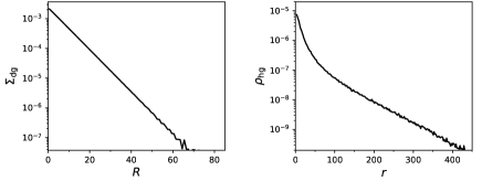
Figure 1.— Left: surface density profile of the gas disk of model L. The surface density $\Sigma_{\rm dg}$ is in the unit of $10^{10}\,h\,{M_{\odot}}\,{\rm{kpc}}^{-2}$, and the cylindrical radius $R$ is in $h^{-1}$ kpc. Right: spherically averaged density profile of the gas halo of model EH. The gas density $\rho_{\rm{hg}}$ is in the unit of $10^{10}\,h^{2}{M_{\odot}}\,{\rm{kpc}}^{-3}$, and the spherical radius $r$ is in $h^{-1}$ kpc.

2.2. Model EH

The ETG model EH is intended to be twice as massive as the LTG model L. The total mass and virial radius of model EH are $177.8\times 10^{10}\,h^{-1}{M_{\odot}}$ and $\sim$175 $h^{-1}$kpc, respectively (Table 1). Model EH is composed of a stellar bulge, DM halo, and gaseous halo.

As in model L, the stellar bulge component has the Hernquist profile (Equation (2)) with a radial scale length of $a_{\rm b}$ = 1.96 $h^{-1}$ kpc. The total mass is $M_{\rm b}=9.8\times 10^{10}\,h^{-1}{M_{\odot}}$, which is two times the total disk-plus-bulge mass of model L.

The DM halo component also follows the NFW profile (Equation (3)) as in model L, with a length scale and the tapering radius of $a_{\rm hd}$ = 17.5 and $b_{\rm hd}$ = 52.5 $h^{-1}$ kpc, respectively. The total mass of the DM halo is $166.32\times 10^{10}\,h^{-1}{M_{\odot}}$.

Unlike in model L, a gas halo component is included in model EH. The gas halo follows an isothermal profile with truncation:

$$\rho_{\rm hg}(r)=\displaystyle\frac{f_{\rm norm}M_{\rm hg}}{2{\pi}\sqrt{\pi}\,b_{\rm hg}}\,\frac{1}{r^{2}+a_{\rm hg}^{2}}\,e^{-(r/b_{\rm hg})^{2}}\,.\\$$ (4)

The core radius is set to $a_{\rm hg}$ = 8.4 $h^{-1}$ kpc, and the tapering radius is chosen to be $b_{\rm hg}$ = 252 $h^{-1}$ kpc. The total mass of the gas halo is $M_{\rm hg}=1.68\times 10^{10}\,h^{-1}{M_{\odot}}$. The halo gas fraction, $f_{\rm hg}=M_{\rm hg}/(M_{\rm hd}+M_{\rm hg})$, is 0.01. The radial density profile of the gas halo is presented in Figure 1 (right panel). The initial temperatures of the gas halo particles are determined by the hydrostatic equilibrium (cf. top row second left panel in Figure 2).

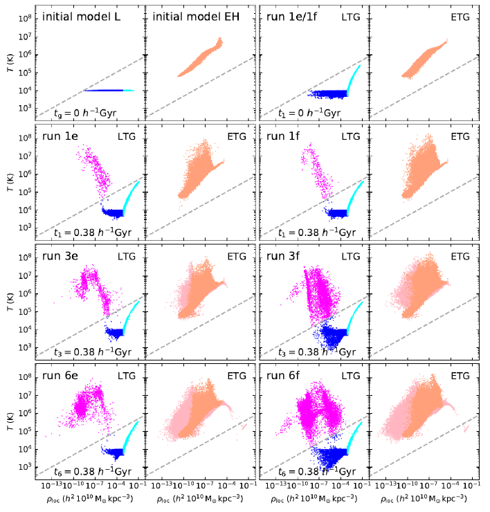
Figure 2.— Temperature ($T$) against local density ($\rho_{\rm loc}$) for the gas particles of the LTG and ETG models. Two top left panels: properties of the disk gas of model L (left panel) and the halo gas of model EH (right panel) in isolation at $t_{\rm g}=0$, i.e., at the time of the realization of each model. The disk gas and halo gas are well separated from each other in the $\rho_{\rm loc}$–$T$ plane by the dashed line. Among the disk gas, the star-forming gas is shown in cyan, and the non-star-forming “cold” gas (lying below the dashed line) is shown in blue. The “hot” halo gas (lying above the dashed line) of model EH is plotted in light brown. Two top right panels: gas properties at $t_{1}=0$, i.e., at the start of runs 1e and 1f. Models L and EH₁ included at this time step for the first-encounter simulations are those evolved in isolation for 0.7 $h^{-1}$ Gyr. The disk gas of model L and the halo gas of model EH₁ are still well separated by the dashed line. Remaining rows: gas properties shortly (0.03 $h^{-1}$ Gyr) after the first, third, and sixth collisions (second, third, and fourth rows, respectively) in the edge-on (left two columns) and face-on (right two columns) cases. (Here $t_{i}$ with ${i}$ = 1, 2, …, 6 represents the time elapsed since the start of the $i$th encounter simulations. The collisions between the LTG and the ETG models in the $i$th-encounter simulations occur at $t_{i}=0.35$ $h^{-1}$ Gyr, refer to Table 2.) Some of the particles originally set as the disk gas of model L have crossed the dashed line and become hot gas (magenta). In the third row, the halo gas particles of models EH₁ and EH₂ are plotted first (pink), and then those of model EH₃ are overplotted (light brown). Similarly, in the fourth row, the halo gas particles of model EH₆ (light brown) are plotted on top of those of models EH₁ through EH₅ (pink). In the bottom two rows, many more hot gas particles of model L (magenta) are seen in the face-on cases than in the edge-on cases.

3. Simulation code

For the simulations of the galaxy–galaxy interactions, we use an early version of the $N$-body/smoothed particle hydrodynamics (SPH) code GADGET-3 (originally described in Springel 2005), the same version of the code as we used in Hwang & Park (2015). Here we briefly describe the simulation code and refer interested readers to Springel & Hernquist (2003) and Hwang & Park (2015) for a more detailed description.

The code uses a tree algorithm (Barnes & Hut 1986) for calculating the gravitational force. For computing the hydrodynamic force, the SPH method in the entropy conservative formulation is adopted with a spline kernel (Gingold & Monaghan 1977; Springel & Hernquist 2002). The radiative cooling and heating are taken into account for the primordial mixture of hydrogen and helium (Katz et al. 1996). Star formation and supernova feedback in the ISM are also implemented using the effective multiphase model of Springel & Hernquist (2003).

For the parameters related to star formation and feedback, we adopt the standard values of the multiphase model in all of our simulations. The star formation time-scale is set to $t_{0}^{\star}=1.5~{}h^{-1}$ Gyr. The mass fraction of massive stars is $\beta=0.1$. The “supernova temperature” and the temperature of cold clouds are $T_{\rm SN}=10^{8}$ and $T_{\rm c}=1000$ K, respectively. The parameter value for supernova evaporation is $A_{0}=1000$.

We set the gravitational softening lengths for the particles in such a way that the maximum acceleration experienced by a single particle is equal in each component. Specifically, the softening lengths for the gas (both halo and disk gas), DM, disk star, and bulge particles are set to 0.077, 0.21, 0.098, and 0.098 $h^{-1}$ kpc, respectively (Table 1).

4. Initial setup of the encounters

The aim of our numerical study is to examine how an LTG (target galaxy) falling into a cluster evolves, particularly through multiple encounters with cluster ETGs possessing hot halo gas. In order to construct the initial conditions (ICs) of our simulations for plausible cases of the interactions, we use the information about the spatial distribution of galaxies drawn from the galaxy catalog of the Coma cluster (H. S. Hwang et al. 2018, in preparation).

In the following subsections, we first explain the Coma cluster catalog and the way we estimate the three-dimensional (3D) volume density of the member galaxies. Then, we describe the procedure to build the ICs for the consecutive collisions between our LTG and ETG models.

4.1. Galaxies in the Coma cluster

The Coma is a well-known nearby cluster at $z$=0.023. The estimated mass, radius, and the velocity dispersion of the cluster are $M_{200}=1.29^{+0.15}_{-0.15}\times 10^{15}\,{M_{\odot}}$, $R_{200}=2.23^{+0.08}_{-0.09}$ Mpc, and $\sigma_{\rm cl}=947\pm 31$ km s^-1, respectively (Sohn et al., 2017).

We have conducted a new redshift survey of the Coma cluster to uniformly and densely cover the cluster region with MMT/Hectospec. We did not use any color selection criteria for spectroscopic targets. By combining with the existing SDSS data in this region (mainly $r$ $<$ 17.77), we could increase the magnitude limit for the redshift data up to $r$ = 20. Among 4761 galaxies with measured redshifts within the radius of 1.9 $h^{-1}$Mpc, we use 1088 member galaxies identified with the caustic technique (Diaferio & Geller, 1997; Diaferio, 1999). The catalog includes right ascension, declination, and projected clustercentric radius, stellar mass, morphological type, Petrosian magnitude, etc. for each member.

In a cluster environment, since most encounters occur at high speed, the ones with less-massive galaxies are not expected to have significant effects on the evolution of the target galaxy. For this reason, given the target as a Milky Way–like LTG, we apply a mass cut to the Coma members. The adopted cut-off is in stellar mass $2.1\times 10^{10}\,h^{-1}{M_{\odot}}$, which is about half the total stellar mass of our LTG model L. With the cutoff, 209 galaxies out of 1088 are selected. These galaxies are only taken into account for the following estimation.

To obtain the 3D distribution of the 209 members, we follow the geometrical deprojection method used in McLaughlin (1999). The geometrical technique is simple and fulfills our need to estimate an approximate number density profile of the cluster. With the assumption of circular symmetry, it gives average volume densities in a number of concentric spherical shells along the 3D deprojected clustercentric radius out of the two-dimensional (2D) projected positions and the number counts listed in the catalog. We describe the procedure for computing the volume densities in Appendix B.

According to the volume density obtained at each shell, we assign the 3D positions of the 209 members by applying a Python module generating a random and uniform distribution. Because of the random feature we use, whenever we generate the 3D distribution of the galaxies, the position of the individual one varies while satisfying the estimated volume density. Thus, to reduce the statistical error, we obtain a total of 100 sets for the 3D distribution of the 209 galaxies and use the median values in our estimation as follows. (It should be noted that our estimation of the 3D distribution of the galaxies is only an approximation because of the small number of galaxies and the random feature we used. Nevertheless, the estimated information is sufficient for our purpose–-i.e., as a reference in constructing plausible ICs for the simulations of the interactions.)

In Figure 3, we show one of the deprojected 3D distribution sets in the $x$–$y$ plane. The orbit of a late-type target galaxy is chosen as a radial path along the $y$-axis, starting from the outer edge $y=1.9~{}h^{-1}$ Mpc to the cluster center $y=0$ (blue line). Because the orbit is the half of the entire path penetrating the cluster radially from one end to another, we consider the galaxies located in the upper hemisphere with $y\geq 0$. Searching for the galaxies lying relatively close to the path, a total of seven galaxies (red circles) are found to be located within 70 $h^{-1}$ kpc of the path (shaded region) in the upper hemisphere. (In the lower hemisphere, four galaxies are found to be situated within 70 $h^{-1}$ kpc of the one end of the path near $y=0$. We do not count them.) The perpendicular distances of these neighboring galaxies to the path are 12, 15, 17, 42, 58, 61, and 67 $h^{-1}$ kpc, from the closest one to the farthest from the path. (Here we consider the completely radial orbit for a simple estimation. The LTG path will actually be deflected by the collisions.)

From the entire 100 sets of the distributions, we search the closest galaxy from the path in each distribution and calculate the median distance of the 100 galaxies. We repeat this for the second-closest galaxy, and up to the sixth-closest galaxy until the median distance does not exceed 70 $h^{-1}$ kpc. The obtained six median values of the distances are 14.6, 24.6, 35.8, 46.3, 53.0, and 61.8 $h^{-1}$kpc, from nearest to farthest. In other words, an LTG moving radially toward the center would likely encounter, on average, six galaxies (with at least comparable masses) at the closest approach distances of roughly 15–65 $h^{-1}$ kpc at intervals of 10 $h^{-1}$ kpc. With the 100 sets, we have checked the tendency that more close encounters are likely to occur near the cluster center where the galaxy number density is highest, and most of the galaxies counted within 70 $h^{-1}$ kpc from the path are an early type. We have also checked the stellar masses of the selected neighboring galaxies from the 100 sets. In some distributions, a couple of very massive neighboring galaxies with stellar masses $\geq 50\times 10^{10}\,h^{-1}{M_{\odot}}$ are found near the center. However, the median values of the stellar masses of all selected neighboring galaxies fall in the range of 4–$5\times 10^{10}\,h^{-1}{M_{\odot}}$ (i.e., about 2–2.5 times the stellar mass of our LTG model). This justifies the mass ratio of our ETG model to LTG of 2:1.

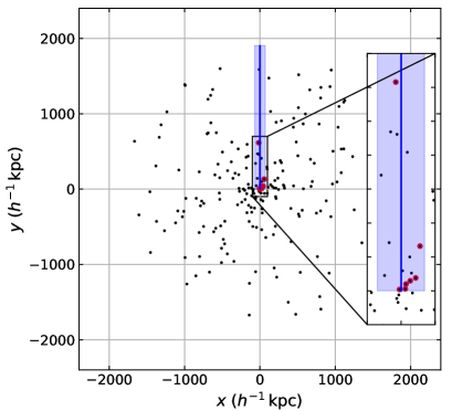
Figure 3.— One of the deprojected 3D distributions of the 209 Coma member galaxies (black dots) shown in the $x$–$y$ plane. The blue line drawn along the $y$-axis, from $y=1900$ to $y=0$ $h^{-1}$ kpc , is chosen for the radial path of an LTG galaxy (target galaxy) falling toward the cluster center. The blue shaded region is the axial cross section of the cylinder with a radius of 70 $h^{-1}$ kpc whose axis and height coincide with the $y$-axis and the orbital path of the target galaxy. Within the cylinder, seven galaxies (red circles) are enclosed in this distribution (see text for more details). The rectangular region $|x|$ $\leq$ $100$ $h^{-1}$ kpc, $-100$ $h^{-1}$ kpc $\leq$ $y$ $\leq$ $700$ $h^{-1}$ kpc is magnified.

4.2. ICs of the encounter simulations

Table 2Runs of the encounters

Runs	LTG Model		ETG Model		At the Closest Approach
	Initial $x$, $y$, $z$	Initial $v_{x}$, $v_{y}$, $v_{z}$	Initial $x$, $y$, $z$	Initial $v_{x}$, $v_{y}$, $v_{z}$	$d_{i}$	$dv_{i}$	$t_{i}$	$t_{{\rm gg}}$	$t_{\rm g}$
	($h^{-1}$kpc)	(km s-1)	($h^{-1}$kpc)	(km s-1)	($h^{-1}$kpc)	(km s-1)	($h^{-1}$Gyr)	($h^{-1}$Gyr)	($h^{-1}$Gyr)
1e, 1f	$-543$, 68, 0	1500, 0, 0	0, 0, 0	0, 0, 0	$d_{1}=65$	$dv_{1}$ = 1569	$t_{1}=0.35$	0.35	1.05
2e, 2f	104, 67, 0	1526, 0, 0	649, 7, 0	0, 0, 0	$d_{2}=55$	$dv_{2}$ = 1583	$t_{2}=0.35$	0.77	1.47
3e, 3f	753, 64, 0	1519, 0, 0	1296, 18, 0	0, 0, 0	$d_{3}=45$	$dv_{3}$ = 1583	$t_{3}=0.35$	1.19	1.89
4e, 4f	1340, 65, 0	1514, 0, 0	1940, 29, 0	0, 0, 0	$d_{4}=35$	$dv_{4}$ = 1586	$t_{4}=0.35$	1.61	2.31
5e, 5f	2042, 65, 0	1500, 0, 0	2579, 42, 0	0, 0, 0	$d_{5}=25$	$dv_{5}$ = 1591	$t_{5}=0.35$	2.03	2.73
6e, 6f	2681, 69, 0	1490, 0, 0	3213, 59, 0	0, 0, 0	$d_{6}=15$	$dv_{6}$ = 1608	$t_{6}=0.35$	2.45	3.15

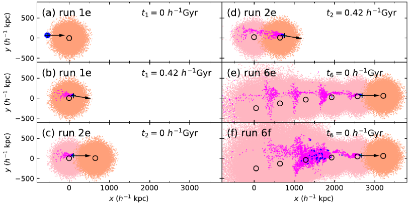
Figure 4.— Distribution of the gas particles of the LTG and ETG models from the encounter simulations seen in the $x$–$y$ plane. The positions of the center of the LTG and each ETG model are marked with a plus and a circle, respectively. The direction of the motion of the LTG model L is indicated by an arrow. The different colors of the gas particles are used in the same way as in Figure 2. (a) Initial configuration of run 1e at $t_{1}$ = 0. Model L has an initial velocity of 1500 km s^-1 in the positive $x$-axis (refer to Table 2). (b) Snapshot of run 1e at $t_{1}$ = 0.42 $h^{-1}$ Gyr, which is 0.07 $h^{-1}$ Gyr after the closest approach between models L and EH₁. The velocity of model L is ($v_{x}$, $v_{y}$, $v_{z}$) = (1524, $-$78, 0) km s^-1, and the direction is facing $\sim$3^∘ below the $x$-axis (the direction and the length of the arrow are not scaled). Model EH₁ is moving slowly with the velocity of ($v_{x}$, $v_{y}$, $v_{z}$) = ($-$12, 42, 0) km s^-1 (the direction of the motion of model EH₁ is not shown). (c) Initial configuration of run 2e at $t_{2}$ = 0. The snapshot of the above panel(b) is rotated $\sim$3^∘ around tje $z$-axis in a counterclockwise direction, and then model EH₂ is included at ($x$, $y$, $z$) = (649, 7, 0) $h^{-1}$ kpc in the rotated coordinate. The direction of motion of model L is now completely horizontal. (d) Snapshot of run 2e at $t_{2}$ = 0.42 $h^{-1}$ Gyr, which is 0.07 $h^{-1}$ Gyr after the closest approach between models L and EH₂. The direction of motion of Model L is slightly below the $x$-axis. (e)–(f) Initial configuration of run 6e and 6f, respectively, at $t_{6}$ = 0. The direction of motion of model L is horizontal. Model EH₆ is included at ($x$, $y$, $z$) = (3213, 59, 0) $h^{-1}$ kpc .

Based on the estimation using the Coma cluster members (explained in Section 4.1), we design the multiple encounters of an LTG with neighboring ETGs using our galaxy models L and EH (Table 2). For a radial orbit from the outskirts to the cluster center, the late-type target galaxy is intended to collide consecutively with six ETGs, first at the closest approach distances of 65 $h^{-1}$ kpc ($d_{1}$) and then at 55 ($d_{2}$), 45 ($d_{3}$), 35 ($d_{4}$), 25 ($d_{5}$), and 15 $h^{-1}$ kpc ($d_{6}$) in order. (Hereafter, we will use the subscripts 1 through 6 to distinguish the distances between the two models (and other quantities) of the first through sixth encounters. For all of the colliding ETGs, the same model EH is used six times and called model EH₁ through model EH₆.) The consecutive encounters are considered for the two different disk tilt angles relative to the orbital direction of the LTG, either edge-on or face-on, keeping all other parameters fixed. Since the ETGs would not affect the LTG significantly at great distances, the ETGs are included one by one in our ICs of the encounter simulations when the LTG approaches each of them relatively closely as follows.

The ICs of the first-encounter simulations for both edge-on and face-on cases (runs 1e and 1f, respectively) are presented in Table 2 and Figure 4(a). Model EH₁ is positioned at the origin, and model L is placed far enough away from the ETG at ($x_{0}$, $y_{0}$, $z_{0}$) = ($-$543, 68, 0) $h^{-1}$ kpc, about three times the virial radius of model EH₁ apart. At the initial time, model EH₁ is stationary and model L has a velocity of ($v_{x0}$, $v_{y0}$, $v_{z0}$) = (1500, 0, 0) km s^-1 in the horizontal direction toward the ETG. Both LTG and ETG models here are included after 0.7 $h^{-1}$ Gyr evolution in isolation. The initial position of model L relative to model EH₁ is chosen so that the two galaxy models encounter most closely with $d_{1}=65$ $h^{-1}$ kpc at $t_{1}=0.35~{}h^{-1}$ Gyr ($t_{1}$ represents the time elapsed since the start of the first-encounter simulations). Figure 4(b) shows the snapshot of run 1e at $t_{1}$ = 0.42 $h^{-1}$ Gyr, shortly after the collision between models L and EH₁. The position ($x$, $y$, $z$) and the velocity ($v_{x}$, $v_{y}$, $v_{z}$) of model L at this time are (108, 61, 0) $h^{-1}$ kpc and (1524, $-$78, 0) km s^-1, respectively. Those of model EH₁ are ($-$4, 4, 0) $h^{-1}$ kpc and ($-$12, 42, 0) km s^-1. The separation between the two models is now 126 $h^{-1}$ kpc, and the direction of motion of model L is slightly ($\sim$3^∘) below the horizontal axis. The second ETG is about to be included at this time step, as explained below.

The ICs of runs 2e and 2f are created by using the snapshots taken at $t_{1}$ = 0.42 $h^{-1}$ Gyr from runs 1e and 1f, respectively. Before putting the second ETG model EH₂ (which is identical to model EH₁ and has evolved for 0.7 $h^{-1}$ Gyr in isolation as well), the snapshots are rotated until the direction of motion of model L becomes completely horizontal (i.e., $\sim$3^∘ around the $z$-axis in the counterclockwise direction). Model EH₂ is then added at the right side of model L, as shown in Figure 4(c) at (649, 7, 0)$~{}h^{-1}$ kpc in the rotated coordinate. (The rotation does not alter the relative positions of the models. It is done solely for convenience in showing the deflection of model L during each encounter simulation.) The position of model EH₂ is chosen so that the closest approach between models L and EH₂ occurs at $t_{2}=0.35~{}h^{-1}$ Gyr with $d_{2}=55$ $h^{-1}$ kpc. The snapshot taken at $t_{2}$ = 0.42 $h^{-1}$ Gyr, shortly after the second collision, is displayed in Figure 4(d). The motion of model L is heading slightly downward below the $x$-axis. The snapshot is rotated again until the direction of model L becomes completely horizontal, and then the third ETG is added at (1296, 18, 0) $h^{-1}$ kpc for the simulations of the third encounter. The above steps are repeated until the sixth ETG is included in the snapshot at $t_{5}$ = 0.42 $h^{-1}$Gyr. Figure 4(e) and (f) present the configuration of the LTG and the six ETGs at the start of the sixth-encounter simulations for the edge-on and face-on cases, respectively.

5. Evolution of an LTG in a cluster environment

As noted earlier, an LTG falling into a cluster will interact with nearby cluster member galaxies and the cluster at the same time. However, taking both galaxy–galaxy and galaxy–cluster interactions into account simultaneously in the hydrodynamic simulations is complicated and overly time-consuming because of the very different scales/properties of the galactic and cluster components (i.e., size, mass, density, temperature, etc). Our simulations focus on galaxy–galaxy interactions with the aim of examining how and to what extent the multiple galaxy interactions can affect the evolution of cluster LTGs. We then compare our simulation results with those of galaxy–cluster interactions. Here we first present our simulation results and then the comparison with others.

5.1. Results of our simulations: effects of multiple galaxy–galaxy interactions

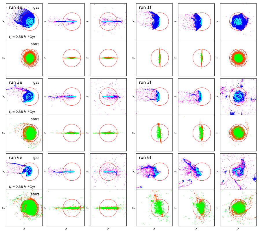
Figure 5.— Distribution of the disk particles of model L at $t_{1}$ = 0.38 $h^{-1}$ Gyr (top two rows), $t_{3}$ = 0.38 $h^{-1}$ Gyr (middle two rows), and $t_{6}$ = 0.38 $h^{-1}$ Gyr (bottom two rows) in the edge-on (left three columns) and face-on (right three columns) cases. The gas and star particles are presented separately (upper and lower panels, respectively) in orthogonal projections. The disk gas particles are displayed with different colors the same way as in Figure 4, i.e., hot non-star-forming gas in magenta, cold non-star-forming gas in blue, and star-forming gas in cyan. The stars originally set as the disk star particles of model L are plotted in orange, and the stars added onto the disk out of the initial disk gas are plotted in green. Each panel measures 100 $h^{-1}$ kpc on a side. A sphere is drawn (red) in the center of the disk with a radius of 24.5 $h^{-1}$ kpc, which enclosed 90% of the disk gas at the initial time $t_{1}$ = 0.

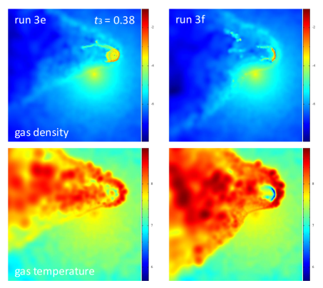
Figure 6.— Log column density (top row) and temperature (bottom row) of the gas components from runs 3e (left column) and 3f (right column) at $t_{3}$ = 0.38 $h^{-1}$ Gyr, projected in the $x$–$y$ plane. Only the gas particles within $\mid{z}\mid\,\leq 10$ are taken into account. Each of the color ranges for the density and temperature are fixed for both edge-on and face-on cases. Each panel measures 300 $h^{-1}$ kpc on a side. This figure is made using SPLASH (Price 2007).

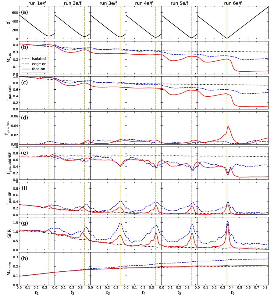
Figure 7.— Variation of some disk quantities throughout the simulations. From left to the right columns, the values obtained from the first-encounter simulations (runs 1e and 1f) through the sixth-encounter simulations (runs 6e and 6f) are displayed. The units are $h^{-1}$ Gyr for time, $h^{-1}$ kpc for distance, $10^{10}\,h^{-1}\,{M_{\odot}}$ for mass, and ${M_{\odot}}$ yr^-1 for SFR. The vertical dashed line drawn at $t_{i}$ = 0.35 $h^{-1}$ Gyr ($i$ = 1, 2, …, 6) in each column indicates the time of the closest approach between models L and EH_i. (a) Distance between model L and model EH_i ($i$ = 1, 2, …, 6) in the $i$th encounter runs. The values from the edge-on and face-on cases are almost equal to each other. (b)–(h) Quantities of the disk particles of model L enclosed within the sphere shown in Figure 5. The dotted, dashed, and solid lines represent the quantities from the isolated, edge-on, and face-on cases, respectively. (b) $M_{\rm gas}$ = total mass of the gas particles (i.e., blue, cyan, and magenta particles enclosed within the sphere in Figure 5). (c) $f_{\rm gas,\,cold}$ = total mass of the cold gas (blue and cyan) / total mass of the gas at $t_{1}$ = 0. (d) $f_{\rm gas,\,hot}$ = total mass of the hot gas (magenta) / total mass of the gas at $t_{1}$ = 0. (e) $f_{\rm gas,\,cold\,NSF}$ = total mass of the cold non-star-forming gas (blue) / total mass of the gas at $t_{1}$ = 0. (f) $f_{\rm gas,\,SF}$ = total mass of the star-forming gas (cyan) / total mass of the gas at $t_{1}$ = 0. (g) SFR = sum of the SFRs of the star-forming gas (cyan). (h) $M_{*,\rm{new}}$ = total mass of the new star particles formed out of the gas (i.e., green particles enclosed within the sphere in Figure 5).

We begin with Figure 2, which shows the evolution of the temperature ($T$) and local density ($\rho_{\rm loc}$) for the gas components of the LTG and ETG models in both edge-on and face-on encounter simulations. The initial values of $\rho_{\rm loc}$ and $T$, at the start of the first-encounter simulations of runs 1e and 1f, are presented in the two top right panels of the figure. At the initial time of $t_{1}=0$, the disk gas particles of model L (left panel) are situated lower right side in the $\rho_{\rm loc}$–$T$ plane. The star-forming gas (plotted in cyan) follows the fingerlike pattern in the higher-density region, which results from the effective equation of state for star-forming gas in the multiphase model (Springel & Hernquist 2003). The halo gas particles of model EH₁ (right panel) are located upper left side in the plane at the initial time. The dashed line is used as a fixed criterion to divide “cold” gas particles (those lying below the line) from “hot” gas particles (those lying above the line) throughout the simulations. At $t_{1}=0$, when the two galaxies have not yet started interactions, the disk gas and halo gas are well separated by the dashed line.

The $\rho_{\rm loc}$–$T$ distribution of the gas shortly after model L collided with models EH₁, EH₃, and EH₆ is shown in the second through fourth rows of Figure 2. Some of the particles initially set as the disk gas of model L are found above the dashed line (magenta dots) in the relatively high-temperature and low-density region, as they are heated and stripped off the disk through interactions with the ETGs. This hot gas appears more as the LTG experiences more collisions and when it flies face-on rather than edge-on.

The snapshots showing the appearance of the gas and the stellar disks of model L at the same times as in Figure 2 are presented in Figure 5. The gas disk forms the bow-like front as it moves fast against the halo gas included in the ETGs (cf. Figure 4). The star-forming gas particles (cyan) are found mostly along the spiral arms and the shock front. They will subsequently turn into stars (green) according to the star formation rates (SFRs) of the gas particles. Some of the disk gas is heated (magenta) and stripped off the disk. The long gas tail developed in runs 3e and 6e (see the $x$–$y$ views) is the result of the shock boundary combined with the clockwise directional rotation of the disk. The corresponding stellar disk, in contrast, forms more symmetrical two-sided tails. Overall, the gas disk shows very different morphology compared with the stellar one, due to hydrodynamic interactions with the halo gas of the ETGs. The offset between the “new” stars (green; stars formed out of the disk gas) and “old” stars (orange; stars originally set as the disk stars) is caused by the shock. Figure 6 more clearly shows the shock that arises from the collision between the gas disk of model L and the gas halo of model EH₃ at $t_{3}$ = 0.38 $h^{-1}$ Gyr, shortly after the third encounter. The shock developed in the face-on case is wider than that in the edge-on case.

In order to examine the evolution of the disk materials, we compute various quantities of the disk particles enclosed within a fixed sphere around the center of the disks over time and present the results in Figure 7. The large circle (red) shown in Figure 5 is the cross section of the sphere with a radius of 4 $\times$ $a_{dg}$, which initially enclosed 90$\%$ of the total mass of the disk gas at $t_{1}=0$. As displayed in Figure 7(b), the LTG loses more disk gas (which is initially set as the disk gas) through the collisions compared with the isolated disk (black dotted line). The disk gas, which is comprised of (cold) star-forming gas, cold non-star-forming gas, and hot (non-star-forming) gas (cf. Figure 2), decreases more severely in the face-on case (red solid line) than in the edge-on case (blue dashed line), in particular, most abruptly after the sixth, deepest collision. The cold gas (star-forming $+$ non-star-forming) fraction also drops shortly after each collision (panel (c)). In the face-on case, the remaining cold gas within the sphere after the sixth collision is only $\sim$10% of the initial value. The hot gas fraction in the edge-on and face-on cases becomes positive due to the collisions, whereas it remains zero in the isolated case (panel (d)). The hot gas fraction rises dramatically near the sixth face-on collision. Among the cold gas, the fraction of non-star-forming gas and star-forming gas decreases and increases in the opposite way near each collision (panels (e) and (f), respectively). The edge-on collisions produce star-forming gas more efficiently than the face-on collisions by inducing successive compression on the disk. By the same token, the SFR in the edge-on case is overall greater than in the face-on case, as well as in the isolated case (panel (g)). The SFR in the face-on case increases only near the collisions and is otherwise similar to that in the isolated case; it finally becomes lower than that in the isolated case after the sixth collision, when the disk loses a significant amount of cold gas. More stars are added onto the disk out of the star-forming gas in the edge-on case than in the face-on and isolated cases (panel (h)).

5.2. Comparison to other simulations: Effects of galaxy–cluster interactions

Here we refer to the numerical study of Jáchym et al. (2007) to compare with ours. The reason we choose this work among many others is because they considered the interactions between an LTG model comparable to ours and a cluster model along a completely radial orbit, just like in our work. They also used the $N$-body/SPH code GADGET (version 1.1; Springel et al., 2001) for the simulations, with some modifications as described below, which allows us more direct comparison.

In Jáchym et al. (2007), the standard galaxy model (“LM” in the paper) is a Milky Way–like model consisting of both stellar and gas disks, a stellar bulge, and a DM halo. (We use their results obtained with only the standard galaxy model LM.) The total disk mass and disk gas fraction are $8.6\times 10^{10}{M_{\odot}}$ and 0.1 in mass, respectively. Their standard cluster model is a Virgo cluster–like model possessing both DM and gaseous halos. The gas component of the hot ICM follows a $\beta$-profile (Equation (4) of the paper) with $R_{\rm{c,ICM}}$ = 13.4 kpc (a parameter of the ICM central concentration) and $\rho_{0,\rm{ICM}}$ = $4\times 10^{-3}\rm{cm^{-3}}$ (the volume density of the ICM in the cluster center). To model a wide variety of clusters from rich ones having a lot of hot gas to poor ones with only a little gas, they vary the values of $R_{\rm{c,ICM}}$ and $\rho_{0,\rm{ICM}}$ from 4 times to a quarter of the standard values, respectively.

They made some modifications in the GADGET code in order to simulate the hydrodynamic interactions between the disk gas and the cluster gas more appropriately. Whereas the original code handles all of the gas particles in one group, the modified code treats the disk and cluster gas as two different groups with different spatial resolution (for details, refer to Section 5 of their paper). This reduces numerical artifacts that can occur when the number densities of the two gas components are significantly different. The numbers of disk gas and cluster gas particles used in the standard models are 12,000 and 120,000, respectively. To achieve a comparable number density for the cluster gas component to that of the disk gas component using the limited number of particles, they kept all of the cluster gas within the 140 kpc radius, applying periodic boundary conditions. (It is not desirable, but rather inevitable to save computational expenses.)

In their simulations, the LTG model moves face-on in a completely radial orbit, from one edge of the cluster model passing the center to the other. The distance from the outskirts of the cluster to the center is 1 Mpc. The times when the LTG enters the ICM region, passes the center, and escapes the ICM region are about 1.52, 1.64, and 1.76 Gyr, respectively, since the start of the run. The velocity when it passes the center of the cluster is about 1300 km s^-1. In the run passing through the standard cluster model, the LTG model turned out to lose about one-third of its original disk gas by the end of the run at 2 Gyr. More specifically, the LTG model continues to lose its gas until just after it passes the cluster center. The minimum mass of the gas disk ($M_{\rm min}$), measuring the gas within $\pm 1$ kpc from the midplane of the disk, is 49 % of the original mass about 20 Myr after it passes the center. After the minimum, much of the stripped gas become accreted back onto the disk. The mass of the reaccreted gas ($M_{\rm accr}$) is 22 % of the original disk mass. Thus, the mass of the stripped gas ($M_{\rm strip}$) is 29 % of the initial mass of the gas disk (cf. $M_{\rm min}$ + $M_{\rm accr}$ + $M_{\rm strip}$ = 100 %).

In the run with the cluster model containing the richest ICM (having four times greater values of $R_{\rm{c,ICM}}$ and $\rho_{0,\rm{ICM}}$ than those of the standard cluster model), $M_{\rm min}$, $M_{\rm accr}$, and $M_{\rm strip}$ are 15 %, 0 %, and 85 %, respectively. In the opposite case, with the poorest ICM in the cluster model, $M_{\rm min}$, $M_{\rm accr}$, and $M_{\rm strip}$ are 84 %, 15 %, and 1 %, respectively.

Considering the fact that their standard cluster model is designed to represent a Virgo-like cluster, the ICM is confined within the sphere of the radius 140 kpc, and the maximum relative velocity of the LTG model is about 1300 km s^-1 (which is about 300 km s^-1 lower than that of ours), the standard cluster run may not be equivalent to make a comparison with our results, although their LTG orbit is a full path from one edge of the cluster model to the other.

Instead, their simulation using the cluster model with the richest ICM would be more suitable for the comparison. In both the richest ICM run and our face-on run, the LTGs came out to lose most of the gas through interactions with either the cluster or the six neighboring ETGs with hot gas, respectively. The amounts of the stripped gas obtained from the two runs are almost equivalent to each other, as both fall in the range of 80%–90% of the initial gas. This implies that the impact on disk gas stripping by hydrodynamic interactions with the cluster gas or the hot gas of many neighboring galaxies could be equally significant. Of course, because the distributions of both ICM and member galaxies in a cluster are not uniform, the LTGs in a cluster could evolve very differently, depending on the dynamical histories.

6. Summary and discussion

We have examined the evolution of LTGs in a cluster environment, focusing on the effects of high-speed multiple interactions with cluster ETGs, using $N$-body/SPH simulations. For this, we built the LTG model L having a gas disk and the ETG model EH containing a gas halo, with a total mass ratio of the LTG to ETG of 1:2. Based on the deprojected distribution of the Coma cluster members, we set the ICs of the consecutive collisions of an LTG with six ETGs, at the closest approach distances of 65, 55, 45, 35, 25, and 15 $h^{-1}~{}kpc$ in order, at the relative velocities of about 1500–1600 km $s^{-1}$ for either edge-on or face-on motion of the LTG.

We find that the evolution of an LTG can be significantly affected by high-speed multiple collisions with ETGs, particularly through the hydrodynamic interactions between the cold disk of the LTG and the hot gas halos of the ETGs. The LTG model L loses about half of its initial cold gas after the six collisions in edge-on, while the isolated disk loses about 25 % during the same period (Figure 7 (c)). For the face-on collision case, the cold gas removal from model L during the same period reaches about 90 % of its original gas due to the strongest ram pressure exerted on the disk. The amount of stripped gas obtained from our face-on consecutive run is as much as that found in the simulations of galaxy–cluster interactions of Jáchym et al. (2007), where an LTG (which is comparable with ours) is flying through a cluster with rich ICM (Section 5.2). This means that the evolution of LTGs in a cluster can be strongly affected by the interactions with not only the cluster but also the neighboring galaxies possessing hot gas. Depending on the dynamical history, the LTGs could be more influenced by collisions with neighboring member galaxies.

Our simulations show that star formation is enhanced in the LTG through consecutive high-speed collisions with the ETGs containing hot gas (Figure 7 (g)). For the LTG flying edge-on, not only does the SFR rise near the collisions, it also remains higher at all times than that in the LTG flying face-on. The pressure exerted on the leading side of the edge-on disk by collisions with hot halos subsequently compresses the cold disk more efficiently, leading to more active star formation. In the face-on case, the SFR increases near the collisions, but it decreases again between the collisions down to the level of the isolated one. The SFR in the face-on disk becomes lower than that in the isolated disk after the sixth collision, when the face-on disk loses most of the cold gas that could later participate in star formation.

Because our simulations have not taken a cluster model and the associated effects into account, our results have limitations to be directly compared with the corresponding observational results that bear all of the complex and combined effects over the course of the galaxy life. Nevertheless, our work clearly demonstrates that galaxy–galaxy hydrodynamic interactions can be a major mechanism for changing the properties of cluster LTGs, such as cold gas content and star formation activities. While very fast motion in general of the individual cluster members weakens the effects of the tidal interactions between them, it strengthens the effects of the hydrodynamic interactions. Besides, the frequent encounters between members can make the hydrodynamic interactions more important.

As mentioned in the introduction, some cluster LTGs showing imprints of strong galaxy–galaxy hydrodynamic interactions have also been observed. Some of the cluster LTGs presented in Ebeling et al. (2014; see their Figure 2) might have been influenced by the hydrodynamic interactions with neighboring galaxies as well as the cluster, because the gas tails of the LTGs extend to rather random directions uncorrelated with the deduced projected velocity vectors of the galaxies. In addition, NGC 4438, a highly disturbed LTG in the Virgo cluster, would be a good candidate showing the observational signatures of strong hydrodynamic interactions with the neighboring M86, a bright elliptical galaxy having a hot gas halo. The X-ray-emitting gas plume detected between NGC 4438 and M86 and the spatially coinciding filaments of H$\alpha$ emission support the idea (Ehlert et al., 2013). Besides, Vollmer (2009) showed, for some Virgo cluster LTGs, that the linear orbital segments derived from the dynamical models assuming a smooth, static, and spherical ICM, together with the ICM density distribution derived from X-ray observations, give estimates of the ram pressure that are about a factor of 2 higher than those derived from the dynamical simulations for NGC 4501, NGC 4330, and NGC 4569. Vollmer (2009) also showed that compared to these galaxies, the two LTGs near M86, NGC 4388 and NGC 4438, require a still 2 times higher peak ram pressure than expected from a smooth and static ICM, assuming an even higher stripping efficiency and/or ICM density. We also argue that, by taking the effects of the hydrodynamic interactions with neighboring galaxies into account, the discrepancy could be solved.

We end this work by emphasizing the importance of galaxy–galaxy hydrodynamic interactions in order to better understand the distinctive properties of the galaxies in the cluster environment, such as the morphology-radius or morphology-density relation. From a numerical aspect, more high-quality hydrodynamic simulations resolving both galactic and intracluster gas in comparable resolutions would be more effective to unveil the evolution of the galaxies in a cluster. Simulations with well-constrained ICs considering the cluster and all of the members orbiting in it together would be most desirable.

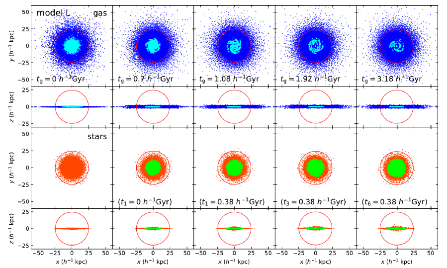
Figure 8.— Five snapshots of the distribution of the disk particles of the isolated model L at $t_{\rm g}$ = 0, 0.7, 1.08, 1.92, and 3.18 $h^{-1}$ Gyr. The gas and stellar particles are displayed with different colors in the same way as in Figure 5: cold non-star-forming gas in blue, star-forming gas in cyan, old disk stars in orange, and stars newly formed out of the gas in green. The large circle shown in each panel is the cross section of the sphere as in Figure 5, which encloses 90 % of the total disk gas in mass at $t_{\rm g}$ = 0.7 $h^{-1}$ Gyr. The times of the second through fifth snapshots correspond to $t_{1}$ = 0, $t_{1}$ = 0.38, $t_{3}$ = 0.38, and $t_{6}$ = 0.38 $h^{-1}$ Gyr, respectively (written in parentheses in the third row; refer to Table 2).

We run each of our models in isolation over 5 $h^{-1}$ Gyr and check the stability. The total energy and angular momentum of the models are well conserved, particularly with almost no change since the first few hundred Myr through the end of the runs. In Figure 8, we show the evolution of the star and gas disks of the LTG model L, where more interesting phenomena occur on the disks, in contrast to the ETG model EH. The star-forming gas (cyan) subsequently turns into stars (green), and the spiral arms and the bar develop on the disks. To minimize any initial fluctuations in our models, both models L and EH at the time of the second snapshot are included in the ICs of our encounter simulations.

APPENDIX B

DEPROJECTION METHOD

We adopt the geometrical deprojection algorithm of McLaughlin (1999) to obtain an approximate 3D distribution of the 209 galaxies in the galaxy catalog of the Coma cluster (H. S. Hwang et al. 2018, in preparation). The geometrical technique makes only one assumption of circular symmetry, in contrast to an Abel integral, which requires the appropriate fitting function for the density of the cluster. We calculate the average volume densities ($n_{\rm{cl}}$) for a number of concentric spherical shells, which are divided along the 3D radii of the cluster as follows.

First, we count the number of member galaxies in every interval, $dR$, of the 2D projected clustercentric radius $R$. As illustrated in Figure 11 in McLaughlin (1999), let the projected radius at each boundary of the cylindrical bins be labeled as $R_{0}$, $R_{1}$, $R_{2}$, …, $R_{m}$ from the center to the outer edge. (The outermost $R$ in the figure is labeled $R_{2}$, which corresponds to $R_{m}$ in our description.) We also divide the cluster into spherical shells at every $dr$ of the 3D deprojected clustercentric radius $r$ and label them $r_{0}$, $r_{1}$, $r_{2}$, …, $r_{m}$. Choosing the same value for both $dR$ and $dr$ makes $r_{0}=R_{0}$, $r_{1}=R_{1}$, and so on.

For the outermost cylindrical bin $R_{m-1}\leq R\leq R_{m}$, because all of the galaxies observed within the cylinder should be located in the outermost spherical shell $r_{m-1}\leq r\leq r_{m}$, the deprojected volume density $n_{\rm cl}$ at the outermost shell can easily be calculated as the number count at the cylinder $R_{m-1}\leq R\leq R_{m}$ divided by the volume of the shell $r_{m-1}\leq r\leq r_{m}$, which is intersected by the cylinder $R_{m-1}\leq R\leq R_{m}$ (i.e., the hatched regions between $R_{1}$ and $R_{2}$ in the figure). Moving inward to the second outermost cylinder $R_{m-2}\leq R\leq R_{m-1}$, the number count at the cylinder includes the contributions from both the outermost spherical shell and the second outermost shell. Given the volume density at the outermost shell, the volume density at the second outermost shell can be obtained by solving the generalized equation A2 of McLaughlin (1999). The volume density at all other shells, from the outside in, can also be calculated by using the same equation.

We try several different values for $dR$, ranging from 0.1 to 0.5 $h^{-1}$ Mpc. Some of them result in negative values of $n_{\rm cl}$ or very small values for certain spherical shells due to the limited number of sample galaxies. Choosing $dR$ = 0.3 $h^{-1}$ Mpc, we get all positive and reasonably smooth values for $n_{\rm cl}$. The obtained average number densities at the innermost shell through the outermost one are 37, 29, 31, 20, 41, 32, and 19, respectively.

APPENDIX C

RESOLUTION TEST

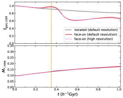
Figure 9.— Time evolution of the cold gas fraction (top panel) and the total mass of the newly formed stars (bottom panel) on the disk of the LTG model from the resolution test runs. The disk quantities (as in Figure 7 (c) and (h)) are measured within the spherical volume, which had initially enclosed 90% of the disk gas (as drawn in Figure 5). The stellar mass is in units of $10^{10}\,h^{-1}\,{M_{\odot}}$. The values obtained from the default and high-resolution encounter runs are displayed with solid and dashed lines, respectively. Those obtained from the isolated case with the default resolution are shown with dotted lines for comparison. The vertical dashed line indicates the closest approach time between the LTG and ETG models, $t$ = 0.35 $h^{-1}$ Gyr.

In order to check whether our simulation results are robust to changes in resolution, we build our LTG and ETG models with higher resolution as well, using four times the number of particles for all components as those listed in Table 1 (“default” resolution) and keeping all other parameters fixed.

As the resolution test, we run an LTG-ETG encounter simulation twice, first with the default resolution models and then with the high-resolution models. The initial configuration of the LTG and ETG models is as follows. Model L is initially placed at ($x_{0}$, $y_{0}$, $z_{0}$) = ($-$545, 38, 0) $h^{-1}$ kpc and flies face-on with a velocity of ($v_{x0}$, $v_{y0}$, $v_{z0}$) = (1500, 0, 0) km s^-1; model EH is initially positioned at the origin with zero velocity. After 0.35 $h^{-1}$ Gyr (since the start of each run), models L and EH encounter most closely at a distance of 35 $h^{-1}$ kpc.

In Figure 9, we show the time evolution of the cold gas fraction (top panel) and the total mass of the newly formed stars (bottom panel) from the default and high-resolution runs. We find that the values match each other well overall, and the main results of our simulations remain consistent in the different resolution runs.

APPENDIX D

GAS CONTENT OF THE LTG IN DIFFERENT SITUATIONS

We perform three runs, “D”, “Cv”, and “Cd”, to compare the evolution of the gas content of an LTG encountering an ETG at the closest approach distance of 35 $h^{-1}$ kpc. (i) Run D is the default resolution run that is described in Appendix C. (ii) Run Cv is the same as run D, except with the initial velocity of model L. It is $v_{x0}$ = 2500 km s^-1 in run Cv, which is about 1.7 times faster than that in run D. (iii) In run Cd, the LTG model L collides with the different ETG model “EH^′”. The initial positions and velocities of both models are identical to those of run D. Model EH^′ is designed to have a gas halo twice as massive as that of model EH. The total masses of the gas and the DM halos of model EH^′ are $M_{\rm hg}=3.36\times 10^{10}$ and $M_{\rm hd}=164.64\times 10^{10}\,h^{-1}{M_{\odot}}$, respectively. All other model parameters are the same as those of model EH (Table 1). The radial density profiles of the gas halos of models EH and EH^′ are presented in Figure 10.

The ram-pressure force exerting on the gas disk of the LTG, which flies face-on through the hot halo of the ETG, is proportional to the mass density of the gas halo and the square of the relative velocity of the LTG with respect to the ETG. Thus, the strength of the ram pressure on the gas disk is expected to be strongest in run Cv, second-strongest in run Cd, and weakest in run D. Figure 11 presents the evolution of the cold gas fraction of model L from the three comparison runs. The cold gas (cold non-star-forming gas + star-forming gas) fraction of model L becomes the lowest in run Cv after the collision because of the strongest ram pressure. After the cold gas fraction reaches the minimum, it rises as some of the cold gas that is not completely stripped off the disk falls back onto the disk. This trend appears more strongly in runs Cd and D than in run Cv. The ram pressure on the disk also leads the rise of the star-forming gas fraction near the collision, compared with that of the isolated case.

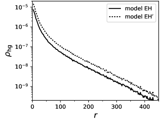
Figure 10.— Spherically averaged density profile of the gas halo of model EH^′ (dotted line) in comparison with that of model EH (solid line). The gas density $\rho_{\rm{hg}}$ is in units of $10^{10}\,h^{2}{M_{\odot}}\,{\rm{kpc}}^{-3}$, and the spherical radius $r$ is in $h^{-1}$ kpc.

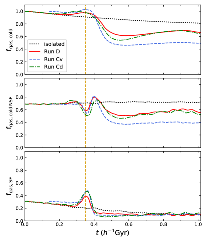
Figure 11.— Time evolutions of the cold gas (cold non-star-forming gas + star-forming gas) fraction (top panel), cold non-star-forming gas fraction (middle panel), and star-forming gas fraction (bottom panel) from the three comparison runs D, Cv, and Cd (solid, dashed, and dot-dashed curves, respectively). The dashed curves for run Cv are shifted along the $x$-axis toward the right by 1.4 $h^{-1}$ Gyr so that the closest approach time between the LTG and the ETG models in run Cv matches with those in runs D and Cd, which is 0.35 $h^{-1}$ Gyr (vertical dashed line).

References

- Abadi et al. (1999) Abadi, M. G., Moore, B., & Bower, R. G. 1999, MNRAS, 308, 947
- Ann (2017) Ann, H.-B. 2017, JKAS, 50, 111
- Barnes (2011) Barnes, J. E. 2011, Astrophysics Source Code Library, record ascl:1102.027
- Barnes & Hibbard (2009) Barnes, J. E., & Hibbard, J. E. 2009, AJ, 137, 3071
- Barnes & Hut (1986) Barnes, J., & Hut, P. 1986, Nature, 324, 446
- Binney & Tremaine (1987) Binney, J., & Tremaine, S. 1987, Galactic Dynamics (Princeton Univ. Press)
- Blanton & Moustakas (2009) Blanton, M. R., & Moustakas, J. 2009, ARA&A, 47, 159
- Boselli & Gavazzi (2006) Boselli, A., & Gavazzi, G. 2006, PASP, 118, 517
- Diaferio (1999) Diaferio, A. 1999, MNRAS, 309, 610
- Diaferio & Geller (1997) Diaferio, A., & Geller, M. J. 1997, ApJ, 481, 633
- Dressler (1980) Dressler, A. 1980, ApJ, 236, 351
- Ebeling et al. (2014) Ebeling, H., Stephenson, L. N., & Edge, A. C. 2014, ApJ, 781, L40
- Ehlert et al. (2013) Ehlert, S., Werner, N., Simionescu, A., et al. 2013, MNRAS, 430, 2401
- Gavazzi et al. (2006) Gavazzi, G., O’Neil, K., Boselli, A., & van Driel, W. 2006, A&A, 449, 929
- Gingold & Monaghan (1977) Gingold R. A., & Monaghan J. J. 1977, MNRAS, 181, 375
- Giovanelli & Haynes (1985) Giovanelli, R., & Haynes, M. P. 1985, ApJ, 292, 404
- Haynes et al. (1984) Haynes, M. P., Giovanelli, R., & Chincarini, G. L. 1984, ARA&A, 22, 445
- Hernquist (1990) Hernquist, L. 1990, ApJ, 356, 359
- Hwang et al. (2010) Hwang, H. S., Elbaz, D., Lee, J. C., et al. 2010, A&A, 522, 33
- Hwang et al. (2012) Hwang, H. S., Park, C., Elbaz, D., et al. 2012, A&A, 538, 15
- Hwang & Park (2015) Hwang, J.-S., & Park, C. 2015, ApJ, 805, 131
- Hwang et al. (2013) Hwang, J.-S., Park, C., & Choi, J.-H. 2013, JKAS, 46, 1
- Jáchym et al. (2007) Jáchym, P., Palous̆, J., Köppen, J., & Combes, F. 2007, A&A, 472, 5
- Katz et al. (1996) Katz, N., Weinberg, D. H., & Hernquist, L. 1996, ApJS, 105, 19
- Koopmann et al. (2006) Koopmann, R. A., Haynes, M. P., & Catinella, B. 2006, AJ, 131, 716
- L’Huillier et al. (2017) L’Huillier, B., Park, C. & Kim, J. 2017, MNRAS, 466, 4875
- Licquia & Newman (2015) Licquia, T. C., & Newman, J. A. 2015, ApJ, 806, 96
- Mastropietro et al. (2005) Mastropietro, C., Moore, B., Mayer, L. Debattista, V. P., Piffaretti1, R., & Stadel, J. 2005, MNRAS, 364, 607
- McLaughlin (1999) McLaughlin, D. E. 1999, AJ, 117, 2398
- McMillan (2011) McMillan, P. J. 2011, MNRAS, 414, 2446
- McMillan & Dehnen (2007) McMillan, P. J., & Dehnen, W. 2007, MNRAS, 378, 541
- Moster et al. (2011) Moster, B. P., Macciò, A. V., Somerville, R. S., Naab, T. & Cox, T. J. 2011, MNRAS, 415, 3750
- Navarro et al. (1996) Navarro, J. F., Frenk, C. S., & White, S. D. M. 1996, ApJ, 462, 563
- Park et al. (2007) Park, C., Choi, Y. Y., Vogeley, M. S., et al. 2007, ApJ, 658, 898
- Park & Hwang (2009) Park, C., & Hwang, H. S. 2009, ApJ, 699, 1595
- Peng et al. (2010) Peng, Y. J.., Lilly, S. J., Kovac̆, K., et al. 2010, ApJ, 721, 193
- Postman et al. (2005) Postman, M., Franx, M., Cross, N. J. G., et al. 2005, ApJ, 623, 721
- Price (2007) Price, D. J. 2007, PASA, 24, 159
- Schulz & Struck (2001) Schulz, S., & Struck, C. 2001, MNRAS, 328, 185
- Sheen et al. (2017) Sheen, Y.-K., Smith, R., Jaffé, Y., et al. 2017, ApJ, 840, L7
- Smith et al. (2013) Smith, R., Duc, P. A., Candlish, G. N., et al. 2013, MNRAS, 436, 839
- Sohn et al. (2017) Sohn, J., Geller, M. J., Zahid, H. J., et al. 2017, ApJS, 229, 20
- Song et al. (2017) Song, H., Hwang, H. S., Park, C., et al. 2017, ApJ, 842, 88
- Springel (2005) Springel, V. 2005, MNRAS, 364, 1105
- Springel & Hernquist (2002) Springel, V., & Hernquist, L. 2002, MNRAS, 333, 649
- Springel & Hernquist (2003) Springel, V., & Hernquist, L. 2003, MNRAS, 339, 289
- Springel et al. (2001) Springel, V., Yoshida, N., & White, S. D. M. 2001, New Astronomy, 6, 79
- Vollmer (2009) Vollmer, B. 2009, A&A, 502, 427
- Vollmer et al. (2001) Vollmer, B., Cayatte, V., Balkowski, C., & Duschl, W. J. 2001, ApJ, 561, 708
- von der Linden et al. (2010) von der Linden, A., Wild, V., Kauffmann, G., White, S. D. M., & Weinmann, S. 2010, MNRAS, 404, 1231
- Whitmore et al. (1993) Whitmore, B. C., Gilmore, D. M., & Jones, C. 1993, ApJ, 407, 489
- York et al. (2000) York, D. G., Adelman, J., Anderson, J. E., et al. 2000, AJ, 120, 1579