Heat Kernel analysis of Syntactic Structures

Abstract.

We consider two different data sets of syntactic parameters and we discuss how to detect relations between parameters through a heat kernel method developed by Belkin–Niyogi, which produces low dimensional representations of the data, based on Laplace eigenfunctions, that preserve neighborhood information. We analyze the different connectivity and clustering structures that arise in the two datasets, and the regions of maximal variance in the two-parameter space of the Belkin–Niyogi construction, which identify preferable choices of independent variables. We compute clustering coefficients and their variance.

1. Introduction: the Geometry of Syntactic Features

The Chomskian Generative Linguistics approach represented the first serious program aimed at a mathematical study of natural languages. The development of the mathematical theory of formal languages, for instance, can be seen as having partly arisen as a spinoff of this program. The aspect of this broad viewpoint that we are more directly interested in here is the concept of syntactic parameters, namely the idea that syntactic structures of natural languages can be “coordinatized” by a set of binary variables. This part of the broader “Principles and Parameters” model of syntax in essence postulates that syntactic structures of natural languages can be fully encoded in a vector of binary variables, which are usually syntactic parameters. The idea goes back to Chomsky’s seminal work [5], [6], and has since played a crucial role in Generative Linguistics. A broad survey of the concept of syntactic parameters is given in [1].

Among the shortcomings of the model is the fact that it has not been possible, so far, to identify a complete set of such syntactic parameters and, even though extensive lists of syntactic features are recorded for a reasonably large number of world languages, it is unclear what relations exist between these binary variables and whether there is a natural choice of a set of “independent coordinates” among them. In other words, the question can be broadly formulated as understanding the geometry of the space of languages, viewed at the syntactic level.

It is in general very difficult for linguists to collect extensive data about syntactic structures for a large number of languages. There are presently some sources of data that we have been using for our investigation. A first source we consider is the “Syntactic Structures of the World’s Languages” (SSWL) database [13], which is freely available as an online resource. The SSWL database has the advantage of being very extensive (presently, it includes 116 parameters and a set of 253 world languages). However, there are issues with these data that need to be taken into account carefully. One problem is linguistic in nature, namely the fact that some of the choices of binary variable recorded in the SSWL database do not reflect what linguists typically consider to be the “true” syntactic parameters, due to conflations of deep and surface structure. The other issue stems from the fact that the parameters in the SSWL database are very non-uniformly mapped across the languages recorded of the database, with some languages 100% mapped with all 116 parameters and others for which only very few of the parameters are recorded. Thus, our data analysis has to take into consideration how to handle the incomplete data. We discuss this issue in §2.1.1. A second recent source of data is given by a list of 83 syntactic parameters for a set of 62 languages (mostly Indo-European) collected by Giuseppe Longobardi, [9], which extends the previously available list of Longobardi and Guardiano [8]. This second list of parameters has several advantages with respect to the SSWL data: the syntactic features considered can be regarded as genuine syntactic parameters; the data are much more uniformly mapped across the set of languages considered, even though some lacunae in the data are still present; some relations between parameters are taken into consideration in the data. The type of relations considered in the Longobardi data are certain forms of entailment according to which some parameters in a language may become undefined by effect of the value of other parameters. This type of relation is recorded in the data using ternary instead of binary values, with $\pm 1$ values corresponding to the usual binary on/off values of a given parameter, and an additional value $0$ to denote the case where a parameter is undefined by effect of the values of one or more of the other parameters. In first approximation, we treat the syntactic features recorded in the data of [9] as an independent set of data with respect to the features recorded in the SSWL database [13].

We will use the term “parameters” in this paper, for simplicity, to denote quite broadly various sets of binary (or ternary, if an “undefined” value is included) variables encoding syntactic features, both in the case of the SSWL data [13] and in the case of the Longobardi data [9].

A natural approach, in order to investigate relations between syntactic parameters at the computational level, is to apply dimensional reduction algorithms to the data and identify possible connectivity and clustering structures. In this paper we focus on a technique developed in [2], [3], [4] based on the differential geometry of Laplacians and heat kernels.

2. Heat Kernel and dimensional reduction

We recall briefly the dimensional reduction technique developed in [2], [3], [4]. The problem addressed by this approach is generating efficient low dimensional representations of data sampled from a probability distribution on a manifold. What one aims for is a method that is generally more efficient at identifying connectivity structures in the data than typical dimensional reduction methods like Principal Component Analysis. The main idea is to build a graph associated to the data points that encodes neighborhood information, and use the Laplacian of the graph to obtain low dimensional representations that maintain the local neighborhood information, constructed using the eigenfunctions and eigenvalues of the Laplacian.

2.1. The Belkin–Niyogi algorithm

The general setting is the following. Consider a collection of data points $p_{1},\ldots,p_{k}$ which lie on a manifold ${\mathcal{M}}$ embedded in a Euclidean space ${\mathbb{R}}^{\ell}$. One wants to find a set of points $y_{1},\ldots,y_{k}$ in a significantly lower dimensional Euclidean space ${\mathbb{R}}^{m}$ (with $m<<\ell$) that suitabely represent the data points $p_{i}$, in the sense that relevant proximity relations are preserved. We assume that the data points $p_{i}$ are binary vectors of syntactic parameters embedded in ${\mathbb{R}}^{\ell}$. Thus, in particular, we can consider the Hamming distance $d_{H}(p_{i},p_{j})$ between data points.

The first step is the construction of an adjacency graph, with vertices given by the data points $p_{i}$ in the ambient space ${\mathbb{R}}^{\ell}$. There are several possible methods for assigning edges in the adjacency graph:

1. $\epsilon$-neighborhood: an edge $e_{ij}$ is assigned between the data points $p_{i}$ and $p_{j}$ iff the distance satisfies

   $$d_{H}(p_{i},p_{j})<\epsilon,$$

2. $n$-nearest neighborhood connectivity: an egde $e_{ij}$ is assigned between $p_{i}$ and $p_{j}$ iff $p_{i}$ is among the $n$ nearest neighbors of $p_{j}$ or viceversa,

3. farthest distance connectivity: a node $p_{i}$ is connected to the $n$ farthest nodes.

The third method has less immediately obvious physical interpretation, but it can be used to isolate highly independent syntactic parameters.

Once an adjacency graph is assigned by one of the methods listed above to the data set, the next step in the Belkin–Niyogi algorithm consists of assigning weights to the edges of the adjacency graph. The weights used in [2], [3], [4] are based on a heat kernel

(2.1) $$W_{ij}=\exp\left(-\frac{\|x_{i}-x_{j}\|^{2}}{t}\right)$$

assigned to an edge $e_{ij}$, with $W_{ij}=0$ if no edge is present between $p_{i}$ and $p_{j}$. The weights depend on a heat kernel parameter $t>0$.

The Laplacian of the graph is defined as the matrix $L=D-W$, where $W=(W_{ij})$ is the $k\times k$ matrix of weights and $D$ is the diagonal matrix with diagonal entries $D_{ii}=\sum_{j}W_{ji}$. One considers the eigenvalue problem

(2.2) $$L\psi=\lambda D\psi$$

where the eigenvalues are listed in increasing order, $0=\lambda_{0}\leq\lambda_{1}\leq\cdots\leq\lambda_{k-1}$ and $\psi_{j}$ are the corresponding eigenvectors, viewed as fuctions

$$\psi_{i}:\{1,\ldots,k\}\to{\mathbb{R}}$$

defined on set of vertices of the graph. One assumes here that the graph is connected, otherwise the same procedure is performed on each connected component.

The following step then consists of mapping the data set via these Laplace eigenfuctions,

(2.3) $${\mathbb{R}}^{\ell}\supset{\mathcal{M}}\ni x_{i}\mapsto(\psi_{1}(i),\ldots,\psi_{m}(i))\in{\mathbb{R}}^{m}.$$

A mapping of the data set to a lower dimensional ${\mathbb{R}}^{m}$ is obtained in this way by using the first $m$ eigenfunctions. That is, the first $m$ eigenvectors $\psi_{j}$, ordered by increasing associated eigvenvalues, form the columns of a $k\times m$ transformation matrix $T$ that transforms the parameter vectors $p=(p_{i})\in\mathbb{R}^{\ell}$ to dimensionally reduced vectors

(2.4) $$p^{\prime}=(p^{\prime}_{j})\in\mathbb{R}^{m}\ \ \ \ \text{ with }\ \ \ p^{\prime}_{j}=\sum_{i}T_{ji}p_{i}.$$

Belkin and Niyogi discussed in [4] the optimality of these embeddings by Laplace eigenfunctions.

2.1.1. Dealing with incomplete syntactic parameter data

To account for the incomplete mapping of languages in both the SSWL database and, to a lesser extent, in the Longobardi data, the data sets used have been filtered. For the SSWL data we considered only those languages for which at least $55\%$ of the parameters are mapped, and for the Longobardi data we only used the languages that are completely recorded ($100\%$ of the parameters mapped). For the graphical methods, we have replaced the remaining missing values in the SSWL data with $0.5$ values, so as not to assume a specific state of the parameter, and so that the frequency of parameter expression is not changed.

3. Connectivity structures of syntactic features

For each data set over $300$ graphs were generated and analyzed. These graphs were used for the clustering and connectivity analysis that we discuss in the next section, to determine structure in the parameter space.

We discuss here a sample of the graphs obtained with the $\epsilon$-neighborhood method and with the $n$-nearest neighborhood method and the possible linguistic implications of the clusters and cliques structures detected.

3.1. Relatedness structures in Longobardi’s syntactic data

We first consider the Longobardi dataset. We construct graphs with the $\epsilon$-neighborhood method for different values of $\epsilon$. The cases shown in Figures 1, 4, 6 show the resulting graphs for $\epsilon=8$, $\epsilon=15$, and $\epsilon=22$, respectively.

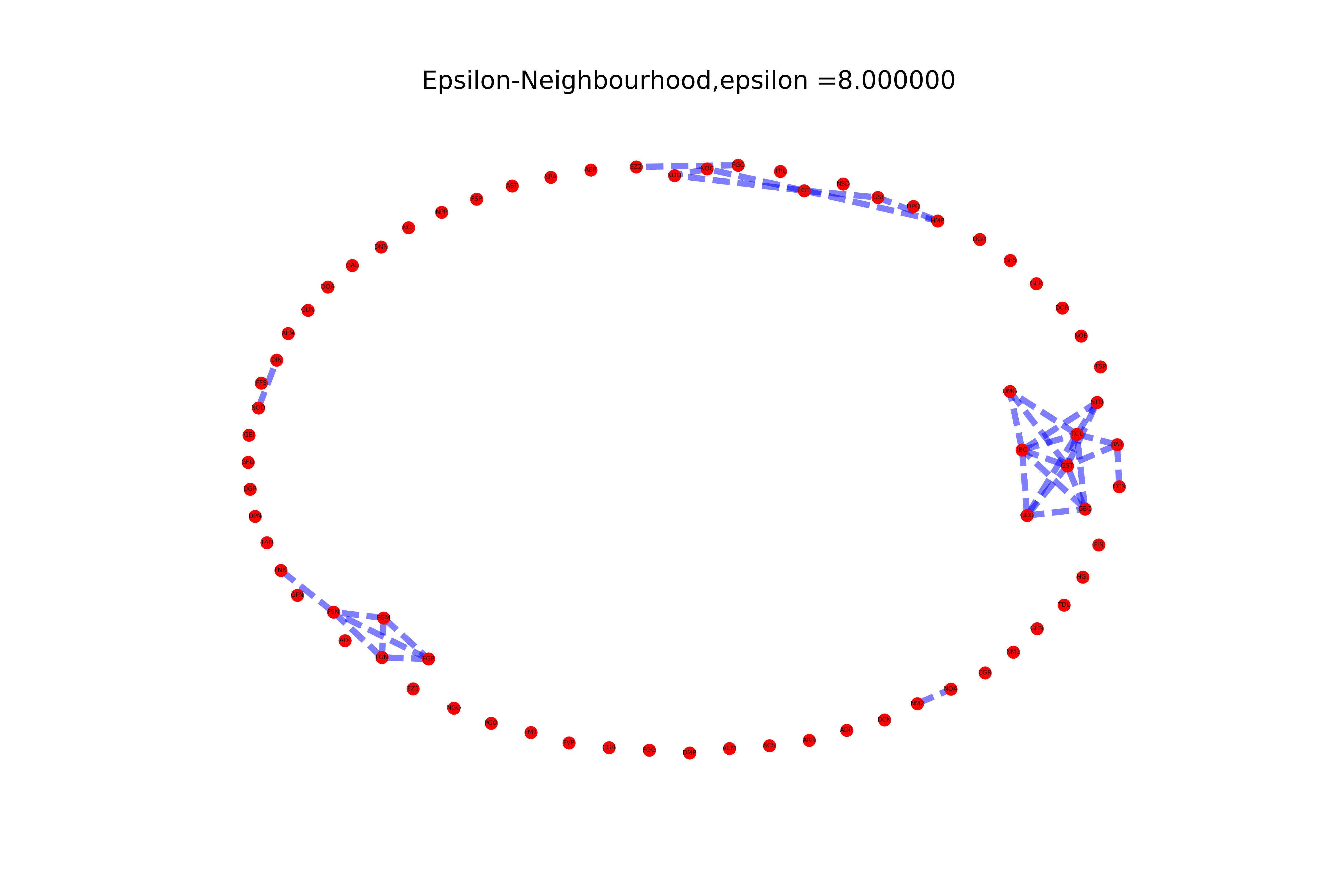
Figure 1. $\epsilon$-neighborhood graph for the Longobardi dataset with $\epsilon=8$.

In this graph one sees five relatedness structures. The two largest structures involve, respectively, $9$ and $7$ vertices, while three smaller relatedness structures involve $5$ vertices and two sets of $2$ vertices. The largest structure consists of the graph shown in Figure 2. The syntactic parameters related by this structure are those listed as DMG (def. matching genitives), GCO (gramm. collective number), GST (grammaticalised Genitive), along with other parameters: BAT, CCN, GBC, IBC, NTD, TCL (see [9] and [7]).

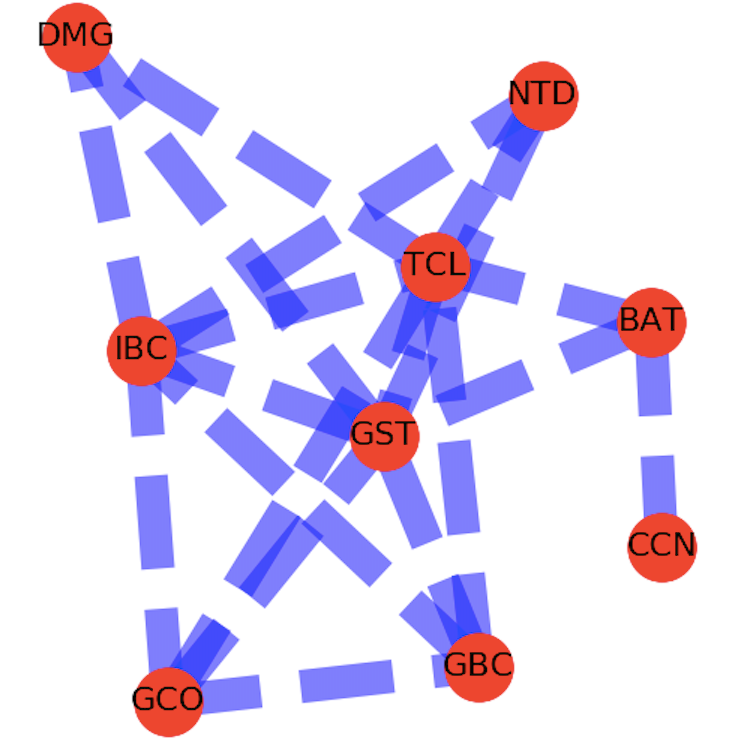
Figure 2. Largest component of $G(\epsilon=8)$ for the Longobardi dataset.

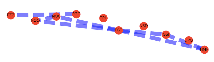
Figure 3. Second component of $G(\epsilon=8)$ for the Longobardi dataset.

The second largest structure in the graph of Figure 1 is the graph shown in Figure 3, which involves the syntactic parameters labelled EZ2 (non-clausal linker), FGC (gramm. classifier), FGT (gramm. temporality), GSI (grammaticalised inalienability), HMP (NP-heading modifier), along with other parameters: NOC, NOO. Note that these two structures appear quite different. If we use the vertex degree (valence) as a simple measure of centrality in a network, then we see that in the graph of Figure 2 the parameters TCL, GST, and IBC have valence $6$, GBC and GCO have valence $4$, and BAT, DMG, and NTD have valence $3$, while only CCN has valence one. Thus, notes in this network tend to have a higher degree of centrality than in the graph of Figure 3, where only the FGT and the NOC parameters have valence $4$, while all the other vertices have valence either one or two. This signals a higher degree of interconnectedness between the first group of syntactic parameters than within the second.

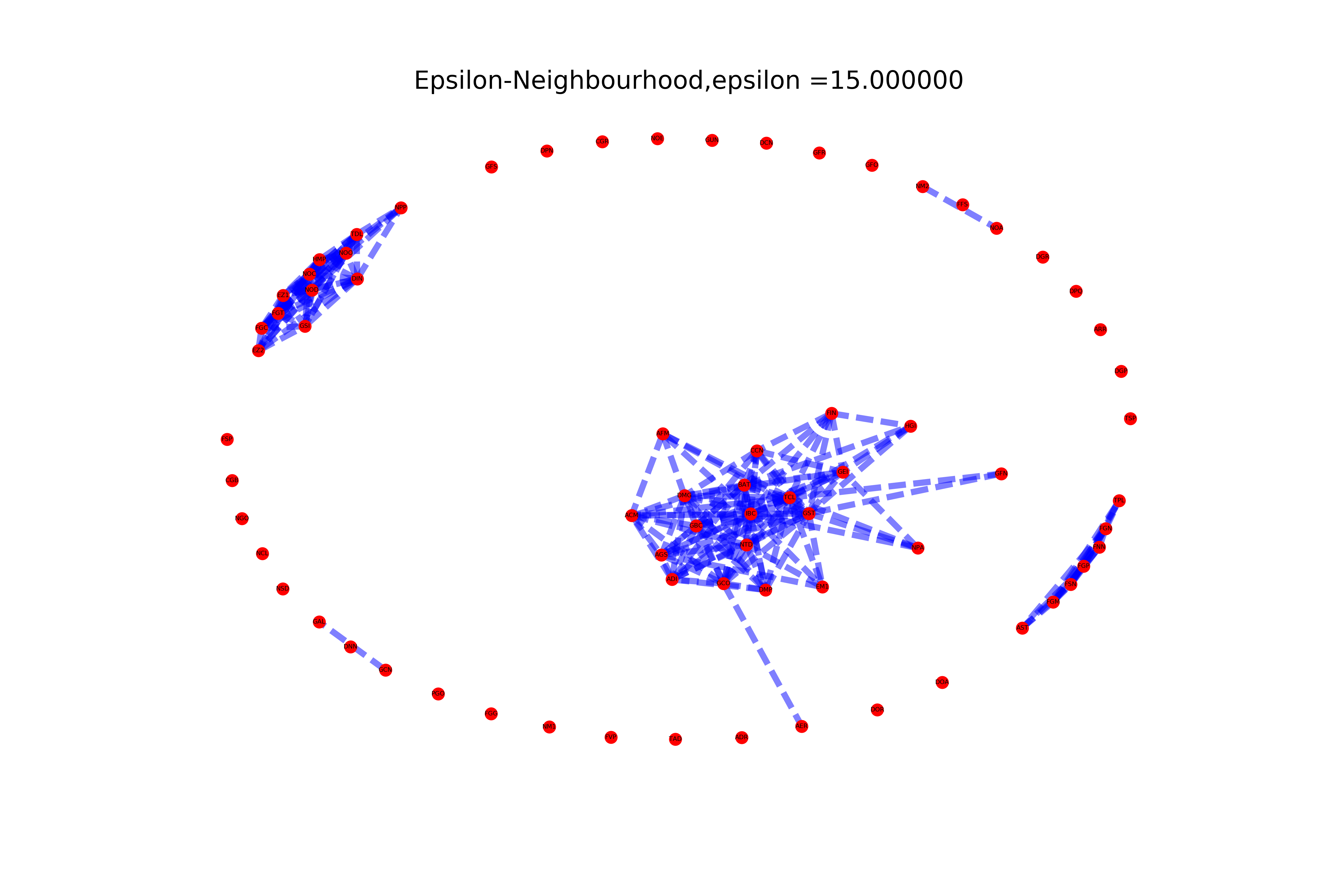
Figure 4. $\epsilon$-neighborhood graphs for the Longobardi dataset with $\epsilon=15$.

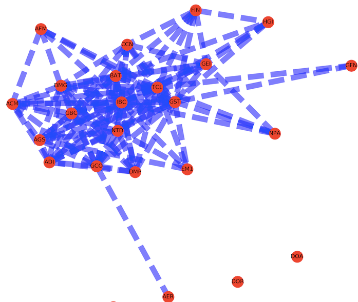
Figure 5. Largest component of $G(\epsilon=15)$ for the Longobardi dataset.

When we increase the $\epsilon$ variable to $15$, we see larger relatedness structures. In particular, we find two interesting networks. The component of Figure 2 has grown into a much larger component, shown in Figure 5, which in addition to the previous vertices BAT, CCN, DMG, GBC, GCO, GST, IBC, NTD, TCL, now includes also ACM, ADI, AER, AFM, AGS, DMP, FIN, HGI, GEI, GFN, NPA. Again, as in the previous case, most of the vertices in this networks have high centrality and only few of them (AER, GFN, NPA) have lower degrees. Those vertices like CCN that were peripheral for the lower value of $\epsilon=8$ in Figure 2 have acquired greater centrality (higher valence) at the scale $\epsilon=15$ in Figure 5. The second largest component involves the nodes DIN, EZ1, EZ2, FGC, FGT, GSI, HMP, NOC, NOD, NOO, NPP, TDL, and includes the network of Figure 3 but where the previous vertices have acquired higher centrality, A third smaller component appears involving connections between the parameters AST (structured APs), FGM (gramm. Case), FGN (gramm. number), FGP (gramm. person), FNN (number on N), FSN (feature spread to N), TPL.

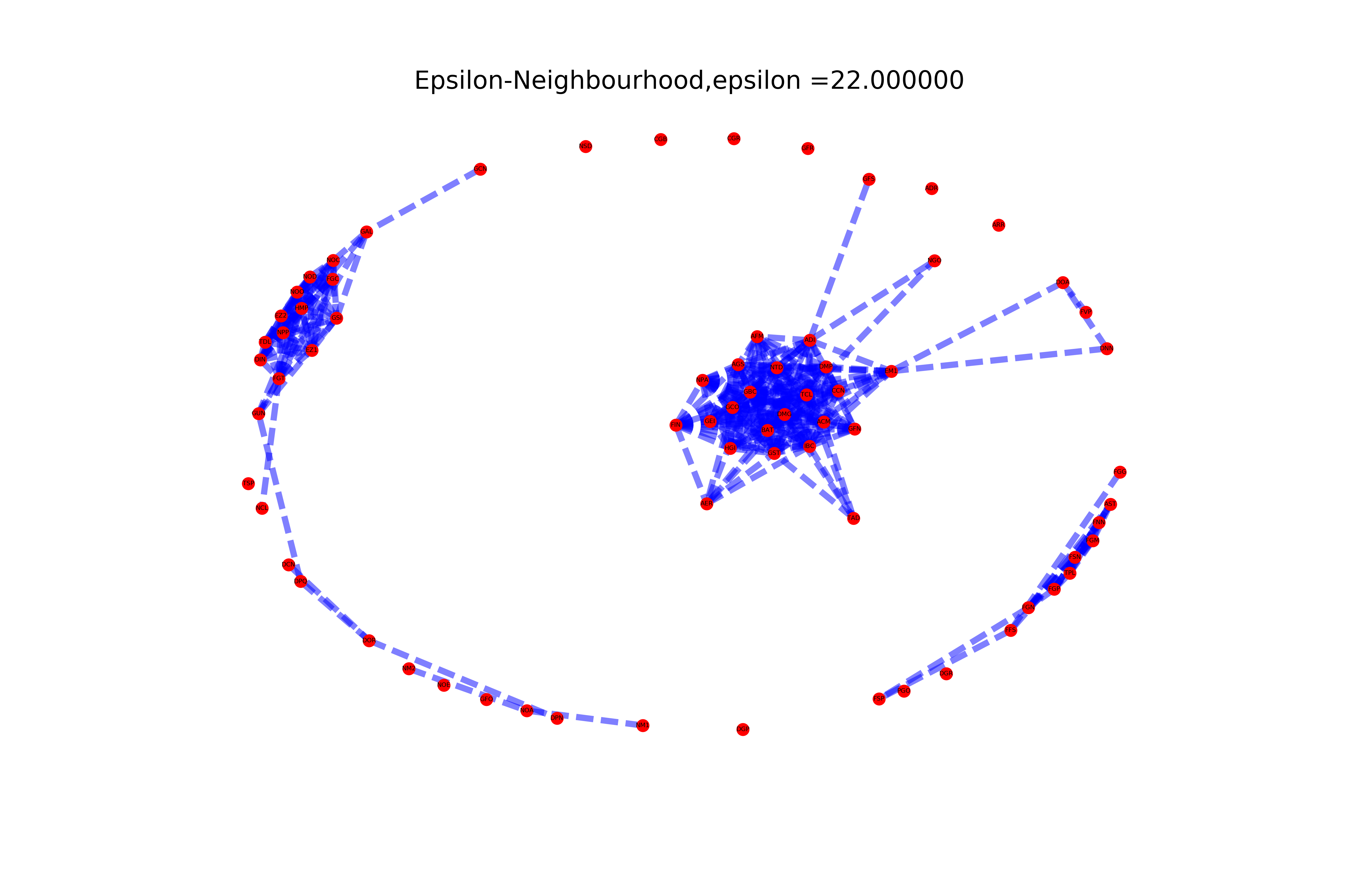
Figure 6. $\epsilon$-neighborhood graphs for the Longobardi dataset with $\epsilon=22$.

When we further increase the neighborhood size variable to $\epsilon=22$, we see that the three main relatedness structures identified above grow in size while still remaining three separate components, Figure 6. These three structures also now clearly differ significantly as network structures in terms of the centrality of nodes. The first component, which grows out of the structure of Figures 2 and 5 involves the nodes ACM, ADI, AER, AFM, AGS, BAT, CCN, DMG, DMP, DNN, DOA, EM1, FIN, FVP, GBC, GCO, GEI, GFN, GFS, GST, HGI, IBC, NGO, NPA, NTD, TAD, TCL. In this component again most of the nodes have a high degree of centrality, with only very few peripheral nodes, such as GFS (valence $1$), NGO, DOA, DNN, FVP (valence $2$), TAD (valence $3$).

The second component, which has grown from the component of Figure 3. Unlike the previous one, this contains a subgraph consisting of nodes with low valence, DCN, DOR, DPN, DPQ, GCN, GFO, NM1, NM2, NOA, NOE, connected through the nodes GUN and GAL to a cluster of high valence, highly interconnected nodes, DIN, EZ1, EZ2, FGC, FGT, GAL, GSI, HMP, NOC, NOD, NOO, NPP, TDL, which contains the original part of the network that already coalesced for smaller values of $\epsilon$.

While the third component grows out of the third component discussed above for the $\epsilon=15$ graph. It involves the nodes AST, FFS, FGG, FGM, FGN, FGP, FNN, FSN, FSP, PGO, TPL. This component also shows typical nodes of lower degrees and a lower interconnectivity.

3.2. Relatedness structures in the SSWL syntactic data

As we discuss more in detail in §4.1 below, connectivity and clustering structures in the SSWL data emerge much more slowly as a function of the neighborhood size $\epsilon$ than in the Longobardi dataset. We can see this for instance in Figure 7, which shows the structure of the SSWL data for the same value $\epsilon=22$ that we used in Figure 6 for the Longobardi data.

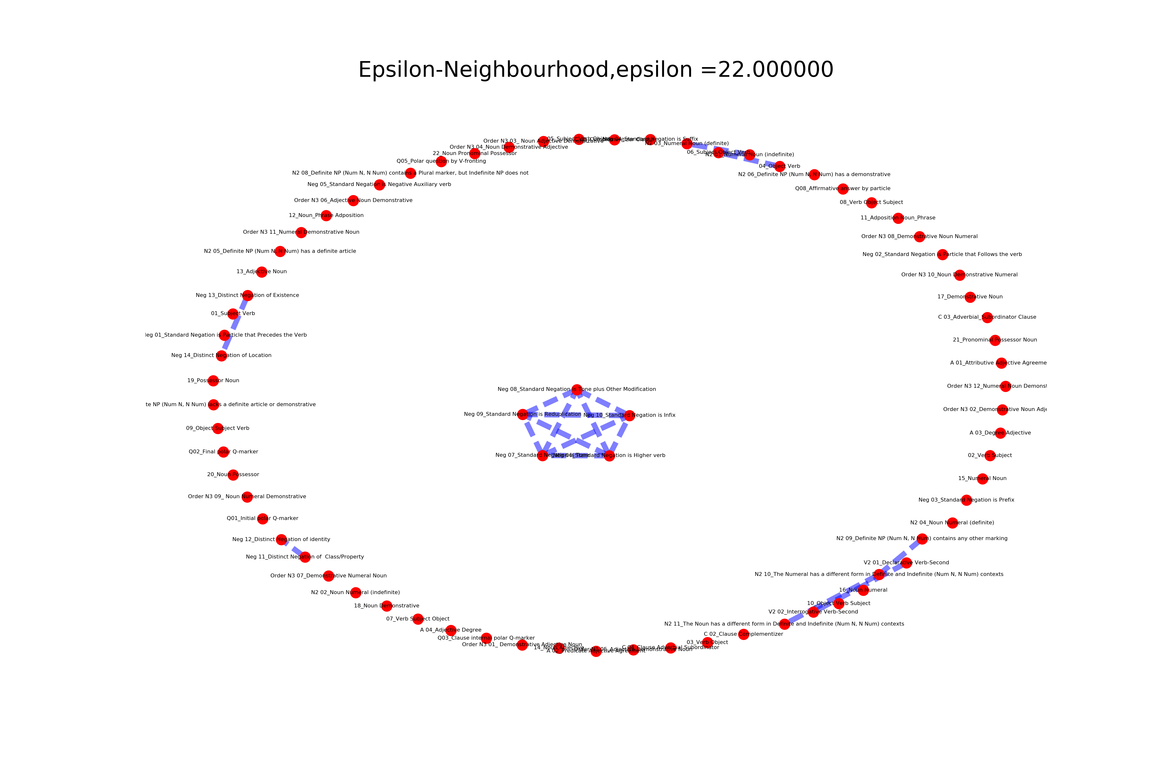
Figure 7. $\epsilon$-neighborhood graphs for the SSWL dataset with $\epsilon=22$.

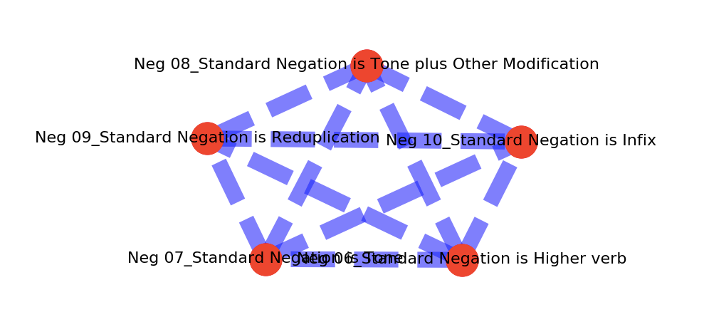
Figure 8. The Standard Negation $\epsilon$-neighborhood graph for $\epsilon=22$.

There are only a few small components visible at this scale in the SSWL data. One component (see Figure 8 is a complete graph on the nodes given by the syntactic features Neg06, Neg07, Neg08, Neg09, Neg10. These features are part of a set of binary variables (Neg01 to Neg10) that describe properties of Standard Negation. It seems interesting that connections between the Neg06 to Neg10 subset emerge earlier (in terms of $\epsilon$-size) than connections with the rest of the parameters in this set. Indeed one can see by computing the graphs at $\epsilon=15$ that the subset Neg07, Neg08, Neg09, Neg10 coalesce into a complete graph on four vertices already at this $\epsilon$-size, while Neg06 becomes connected to this component at a larger size. This subset of the Standard Negation parameters is indeed somewhat different in nature from the Neg01 to Neg05 subset. The first five Standard Negation parameters describe the position of a standard negation particle with respect to the verb (Neg01 and Neg02), whether standard negation is expressed by a prefix or a suffix (Neg03 and Neg04) or through a negative auxiliary verb (Neg05). The remaining set of Standard Negation parameters, which constitute the graph component of Figure 8, instead describe the expression of standard negation through predicate with a subordinate clause complement (Neg06, expressed in Polynesian languages like Tongan), or through tone (Neg07, expressed in Niger-Congo languages like Nupe and Guébie, or in Oto-Manguean languages like Triqui), or tone together with additional modifications to verb form and other constituents in the negated sentence (Neg08, expressed in Niger-Congo languages like Basaa, Igala), by a reduplicated verb form (Neg09, expressed in Niger-Congo languages like Eleme), or by an infix (Neg10, possibly expressed in the Muskogean language Chickasaw). The occurrence of the graph of Figure 8 appears to indicate that these modes of Standard Negation more strongly correlate to one another than the other modes described by the Neg01 to Neg05 variables.

At the scale $\epsilon=22$ there is also a three vertex component involving N2-09, N2-10, N2-11, with one edge between N2-11 and N2-10 and one between N2-10 and N2-09, as well as several components consisting of two vertices joined by an edge, such as V2-01 and V2-02, N2-01 and N2-03, 04 and 06, Neg13 and Neg14, Neg11 and Neg12. The N2-09, N2-10, N2-11 SSWL parameters describe whether the property that the definite NP (noun phrase) contains additional markers which is absent in the indefinite NP (N2-09, expressed in Niger-Congo languages like Basaa, or in the Eastern Armenian language), whether the Numeral has a different form in definite and indefinite contexts (N2-10, expressed in Arabic and Hebrew, in Icelandic and in Arawakan languages like Garifuna), and whether the noun itself has a different form in definite and indefinite contexts (N2-11, expressed for instance in Eastern Armenian, Danish, Icelandic, Norwegian, and in the Sandawe language). The two-vertex component connecting N2-01 and N2-03 also pertain to the same subset of SSWL variables: N2-01 is expressed if at least one numeral can precede the noun in an indefinite NP, while N2-03 is expressed if the same occurs with definite NP.

The parameter Neg13, Distinct Negation of Existence, is expressed in a language when negation of existence differs from Standard Negation (this is expressed in many languages including for instance Arabic and Hebrew, Mandarin, Hungarian, Japanese), while Neg 14, Distinct Negation of Location, is expressed if the negation of predications of location differs from Standard Negation and it also tends to be expressed in the same languages in which Neg13 is expressed. The edge connecting Neg11 and Neg12, on the other hand, connect the Distinct Negation of Class/Property (Neg11, expressed for example in Arabic, Burmese, Fijian, Kiswahili) where negation of predications of class inclusion and property assignments differs from Standard Negation, and Distinct Negation of identity (Neg12, expressed for example in Arabic and Hebrew, or in Indonesian, Thai, Kiswahili) where negation used in predications of identity differs from Standard Negation. At these $\epsilon$-scales these parameters in the Negation sector of the SSWL data do not yet coalesce with the Neg07-Neg10 connected component discussed above. Another single edge component relating V2-01 and V2-02 connects the Declarative Verb-Second property (V2-01, expressed for instance in most Germanic languages, in Estonian, in the Austroasiatic Khasi language, or the Malayo-Polynesian Bajau language) which is expressed when a language allows only one constituent to precede the finite verb in declarative main clauses and the Interrogative Verb-Second (V2-02, expressed for instance in the Germanic languages, in Spanish, Armenian, Georgian, in the Niger-Congo Dagaare language, or the Austroasiatic Khasi language) which is expressed when a language allows only one wh-constituent to precede the finite verb in interrogative main clauses. The fact that the Germanic subfamily of the Indo-European family shares both features may be a factor in driving the connection seen at this scale in the graph. The remaining two vertex connection visible at this $\epsilon$-scale relates the 04 and 06 parameters, that is, Object Verb, expressed when a verb can follow its object in a neutral context, and Subject Object Verb (SOV), expressed when the order Subject Object Verb can be used in a neutral context. Note that other similar pairs in the word order sector of the SSWL database, such as 01 Subject Verb and 05 Subject Verb Object (SVO) do not yes form connected components at these scales, while Object Verb and Subject Object Verb already do. This may reflect the fact that SOV languages are slightly more abundant (around 45$\%$ of world languages) than SVO languages (around 42$\%$ among world languages).

3.3. Nearest neighbor structures in syntactic data

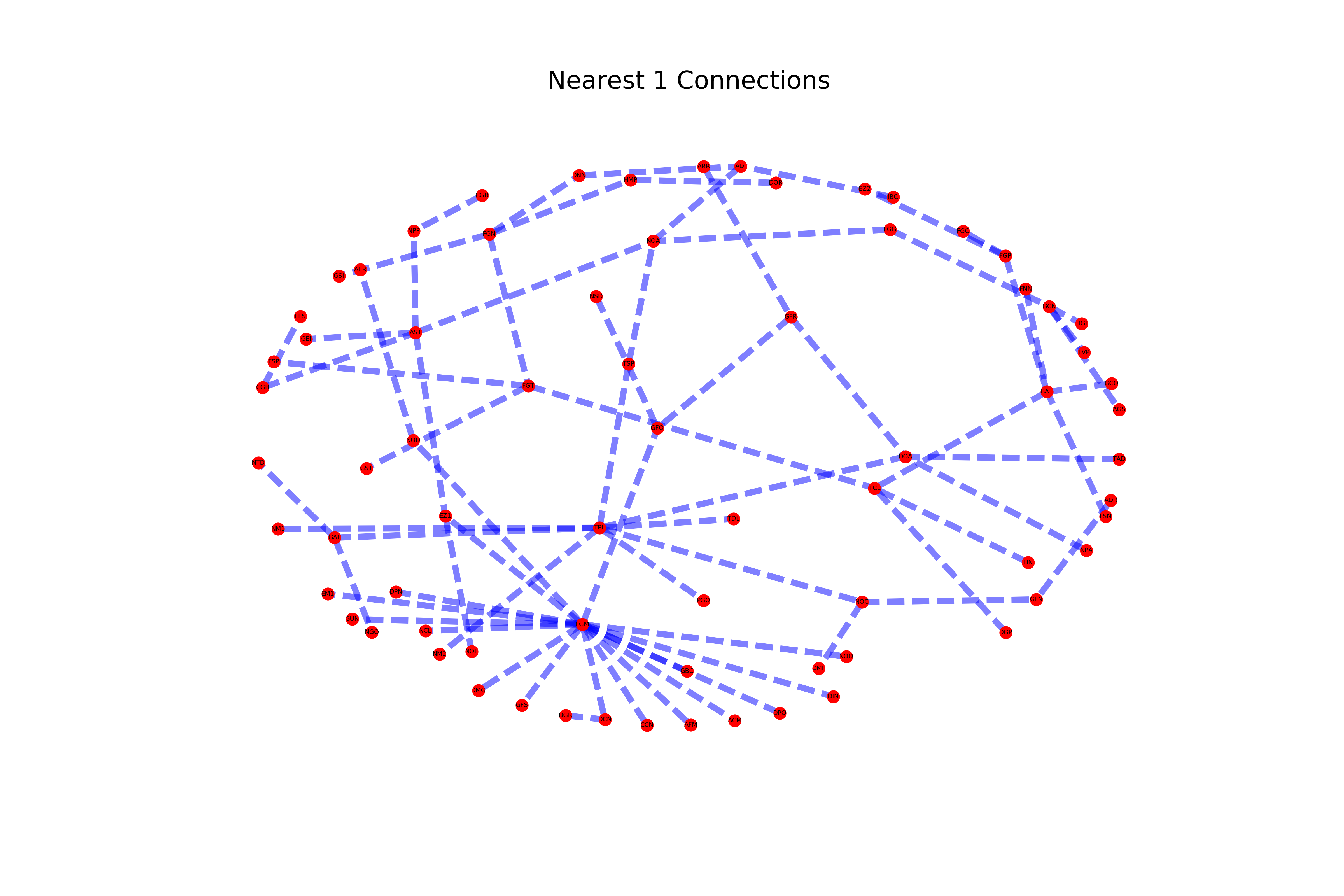
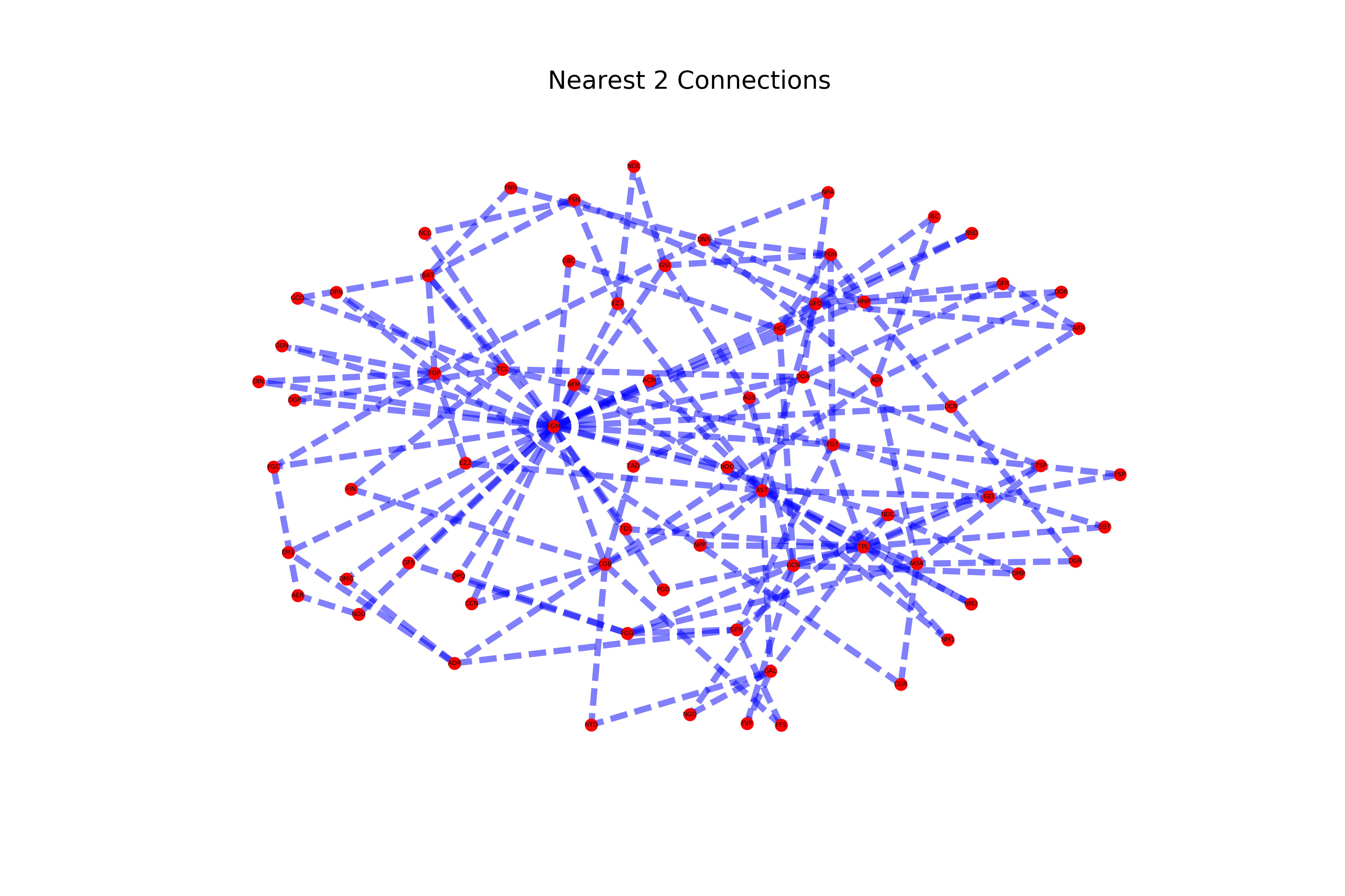
Figure 9. $n$-nearest neighbor graphs for the Longobardi dataset with $n=1$ and $n=2$.

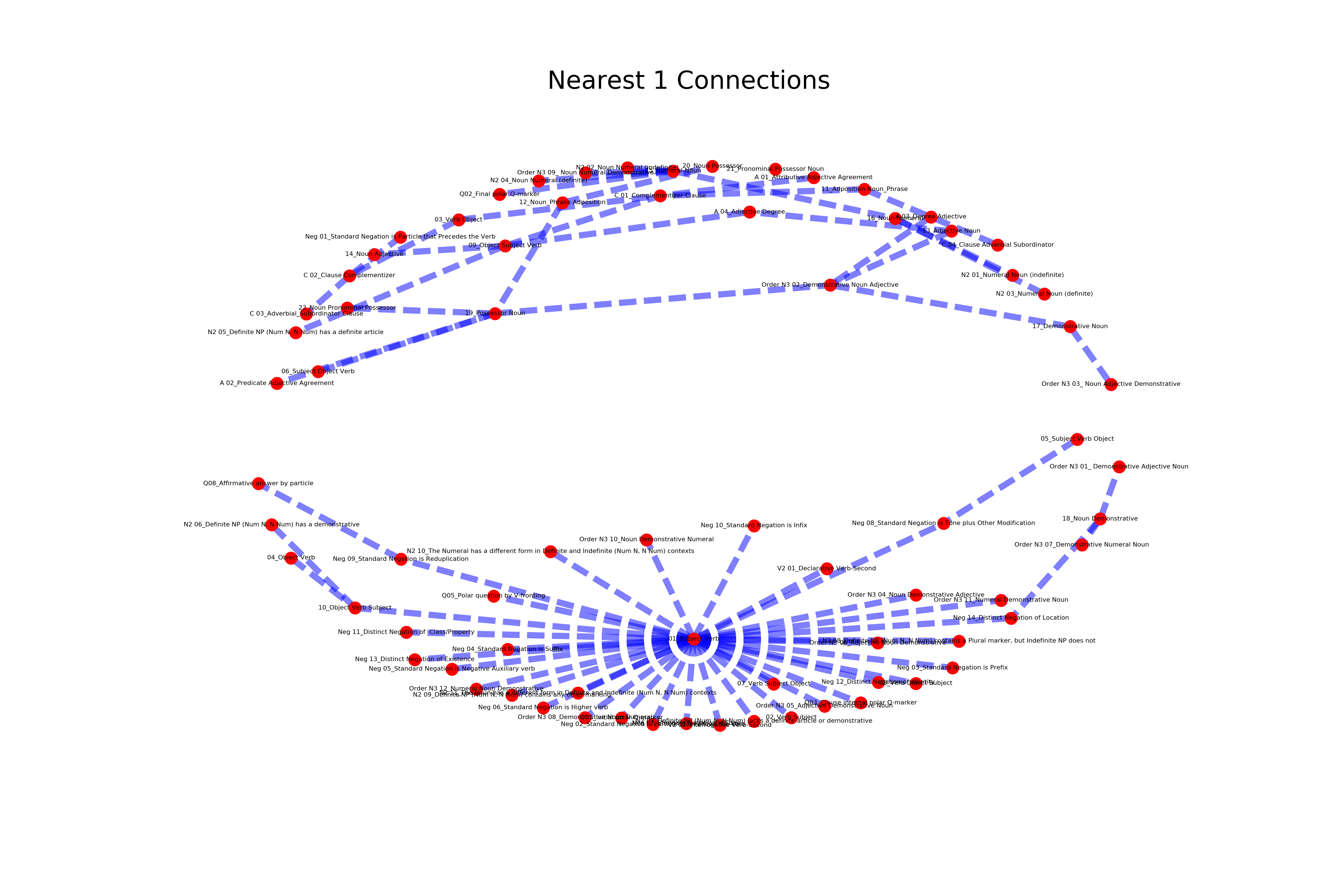
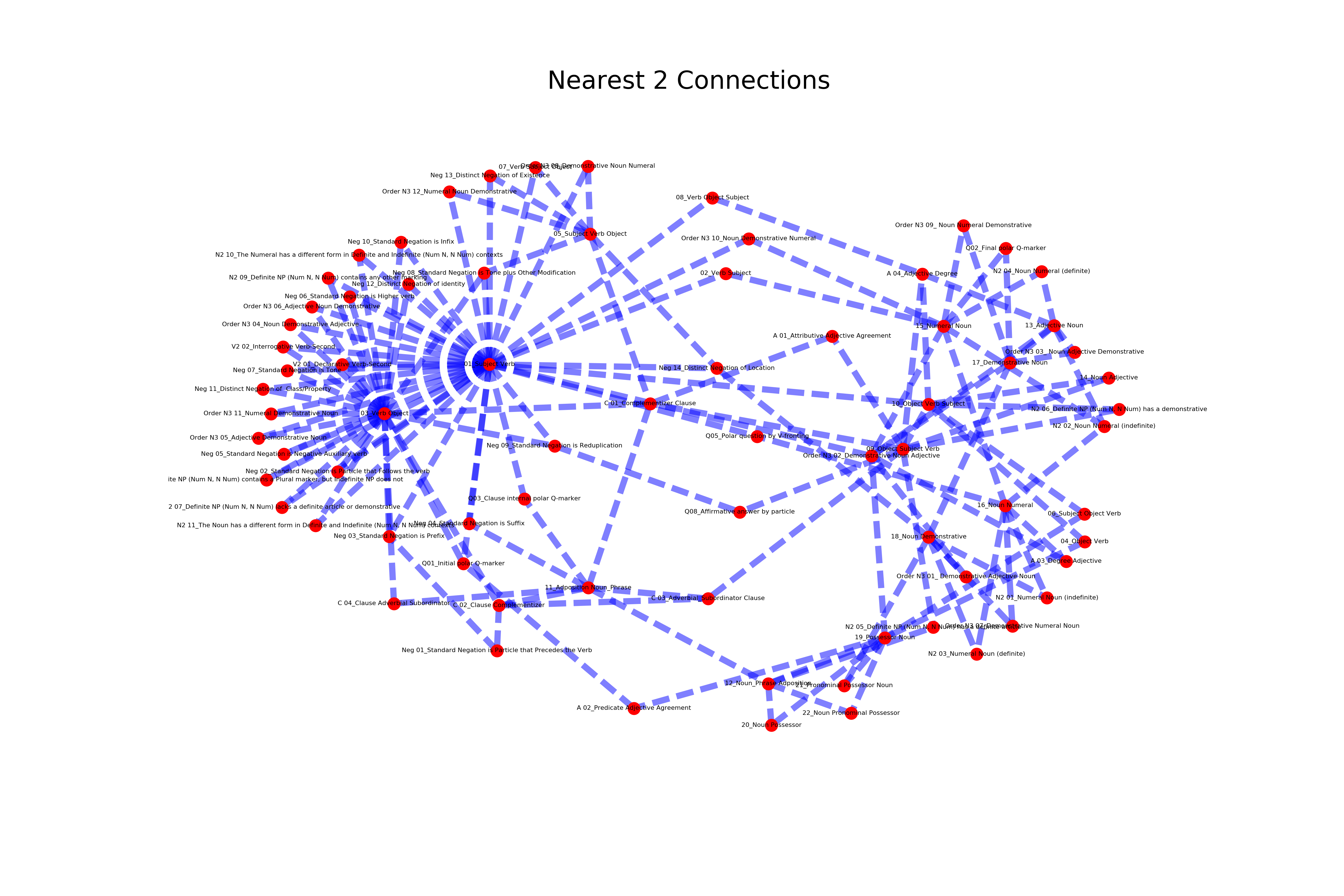
Figure 10. $n$-nearest neighbor graphs for the SSWL dataset with $n=1$ and $n=2$.

As we discuss more in detail in §4.1 below, if we use the $n$-nearest neighbor construction of graphs in the Belkin–Niyogi algorithm instead of the $\epsilon$-neighborhood method, the two sets of data, SSWL and Longobardi’s, tend to behave more similarly.

The nearest one and nearest two connections for the Longobardi dataset are shown in Figure 9. It stands out very clearly that the FGM node (gramm. Case) has a high centrality already at the $n=1$ level, with nodes like AST (structured APs), CGB (unbounded sg N), FGP (gramm. person) and others like TPL, also having high centrality in the network at the $n=2$ level.

A similar analysis of the SSWL data is shown in Figure 10. The type of connectivity structures one sees with this method differ significantly from those obtained by the $\epsilon$-neighborhood approach, discussed above. At the $n=1$ stage, the SSWL data separate neatly into two different connected components. The component shown in the bottom part of the first plot in Figure 10 has a single node of very high centrality, consisting of the 01 Subject Verb parameter, and the rest of the component shows very little interconnectivity. The only nodes in this component that are not directly connected to the central node are Q08 (connected to Neg09), N2-06 and 04 (both connected to 10), 05 (connected to Neg08), Order-N3-01 and Order-N3-07 (both connected to 18), while all other nodes are directly connected to the central 01 Subject Verb node and most of them are valence one. Most strikingly, this component is a tree (trivial first Betti number). This structure may be interpreted as an indicator of an influence of the value of the 01 Subject Verb parameter on the parameters located at all the adjacent nodes.

The other component, shown at the top of the first plot in Figure 10 has a very different structure. It contains no single node of very high centrality and it has a higher degree of interconenctivity (a nontrivial first Betti number). The largest valence of nodes in this component is just $5$ (19 Possessor Noun node); there are a few nodes of degree $4$ (Order-N3-02 Demonstrative Noun Adjectve node, C01 Complementizer Clause node, 09 Object Subject Verb) and of degree $3$ (A03 Degree Adjective, 15 Numeral Noun, 22 Noun Pronominal Possessor). Note how the subdivision of nodes into the two connected components in this $n=1$ graph does not appear to follow any of the natural subdivisions of the SSWL data into different sectors: for example, word order parameters like Subject Verb or Subject Object Verb do not belong to the same component, or the Numeral parameters N2, which fall partly in one and partly in the other component. Negation parameters all belong to the first component (at the bottom of the figure) but they do not form any interconnected structure, unlike the complete graphs in the $\epsilon$-neighborhood picture.

At the $n=2$ level, the two components have already merged. A second high centrality node, 03 Verb Object, has appeared alongside 01 Subject Verb. A large number of nodes are directly connected to these two nodes and to no others.

4. Exploring the $\epsilon$-$t$ space

In this section we discuss how the global clustering and a measure of connectivity for the graphs $G(\epsilon,t)$ generated from the datasets vary with the parameter $\epsilon$. This provides some insight into how the graphs evolve within the Belkin–Niyogi process and at what $\epsilon$-value the graphs stabilize to a complete graph.

4.1. Connectivity and clustering

The measure of connectivity that we consider here is vertex-connectivity, namely the minimum number of nodes that needs to be removed to make the graph disconnected. Clustering, on the other hand, is defined as the mean number of triangular sub-graphs that can be generated from the neighborhood of any given node.

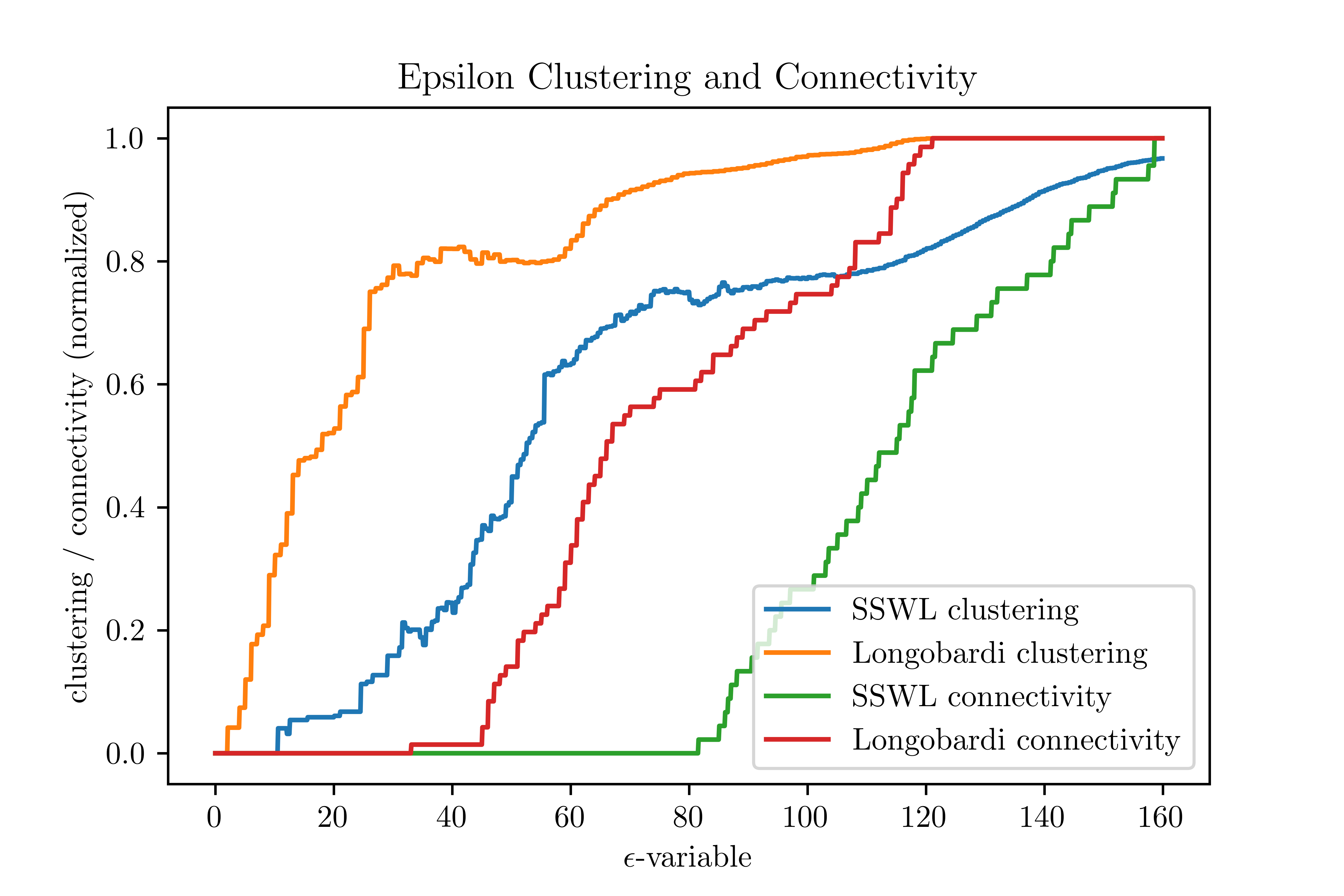
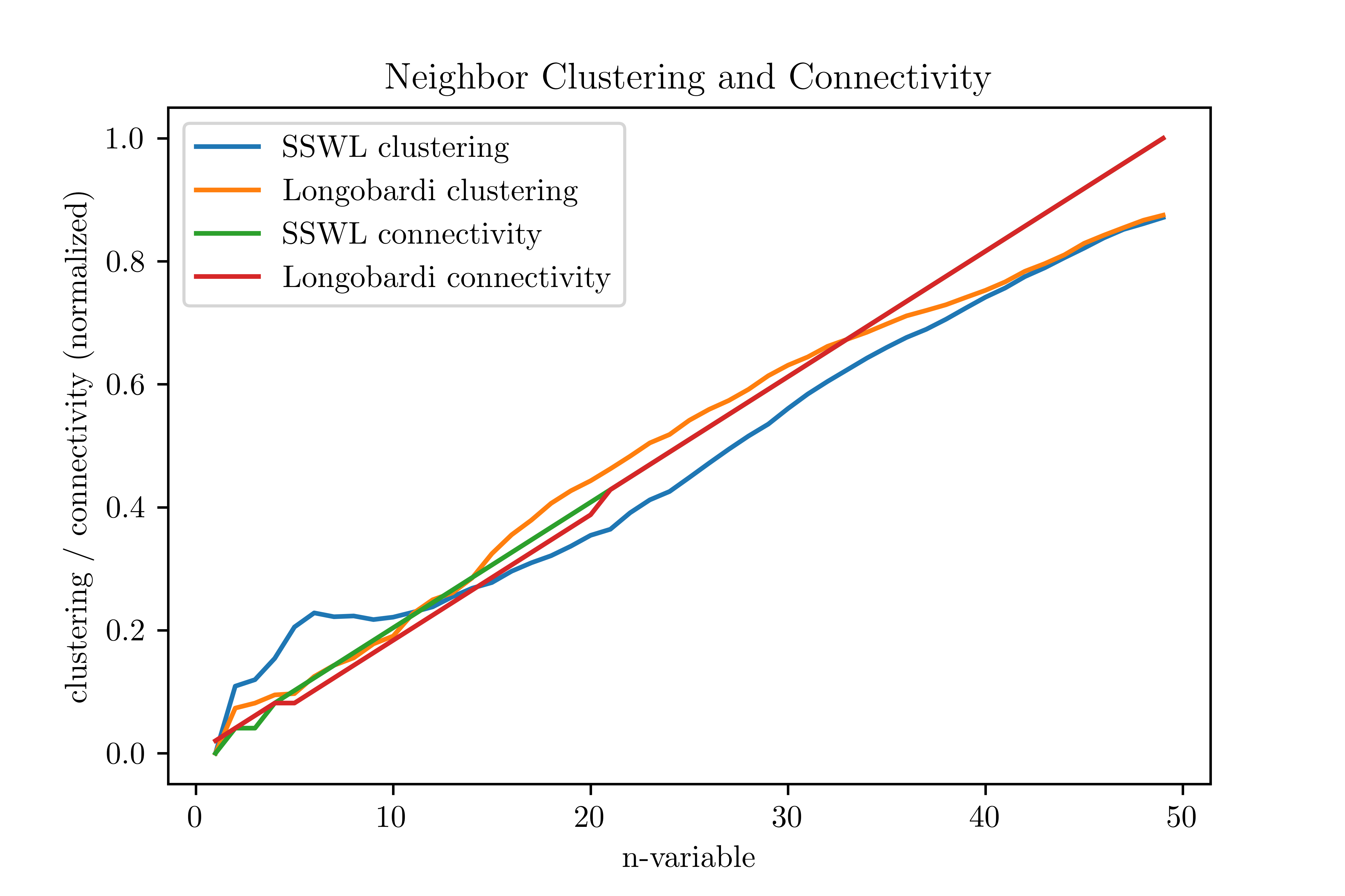
Figure 11. Plots of the connectivity and clustering of graphs as a function of the parameters $\epsilon$ and $n$, respectively, used in the graph generation methods.

The behavior of clustering and connectivity, as a function of either the $\epsilon$-variable in the $\epsilon$-neighborhood construction of the graphs, or of the $n$-variable in the $n$-nearest neighborhood construction shows a significantly different behavior between the SSWL data and the Longobardi data in the the $\epsilon$-neighborhood case, with the SSWL data exhibiting much lower connectivity and clustering than the Longobardi data. On the other hand, the behavior of the two datasets appears much more similar in the $n$-nearest neighborhood case, see Figure 11. If a higher degree of connectivity and clustering is to be taken as an indicator of the presence of relations between the parameters, then the different behavior of the two datasets un the $\epsilon$-neighborhood construction would point to more structured relations in the Longobardi dataset than in the set of syntactic variables reported in the SSWL. As we mentioned above (see [8], [9] for a more detailed explanation), the Longobardi dataset does explicitly record certain types of entailment relations between the listed parameters, so we know a priori that the dataset does not consist of independent variables. Previous analysis, such as [10], also indicated the presence of relations between the SSWL variables, although relations in the SSWL data are not explicitly formulated as the relations recorded in the Longobardi data, and were only detected through a measure of recoverability in Kanerva networks. It is possible that the higher levels of connectivity and clustering visible in the Longobardi data with the $\epsilon$-neighborhood method may reflect the more structured type of relations present in the Longobardi data. It is interesting, though, that when the graph construction is performed using the $n$-nearest neighborhood method, the two datasets tend to behave much more similarly, with the SSWL clustering value peaking above the Longobardi value for small $n$ and trailing slightly below for larger values of $n$.

4.2. Activity regions in the $\epsilon$-$t$ space

We investigate here the simultaneous dependence on both the $\epsilon$-variable of the $\epsilon$-neighborhood construction of the graphs and the $t$-variable of the heat kernel.

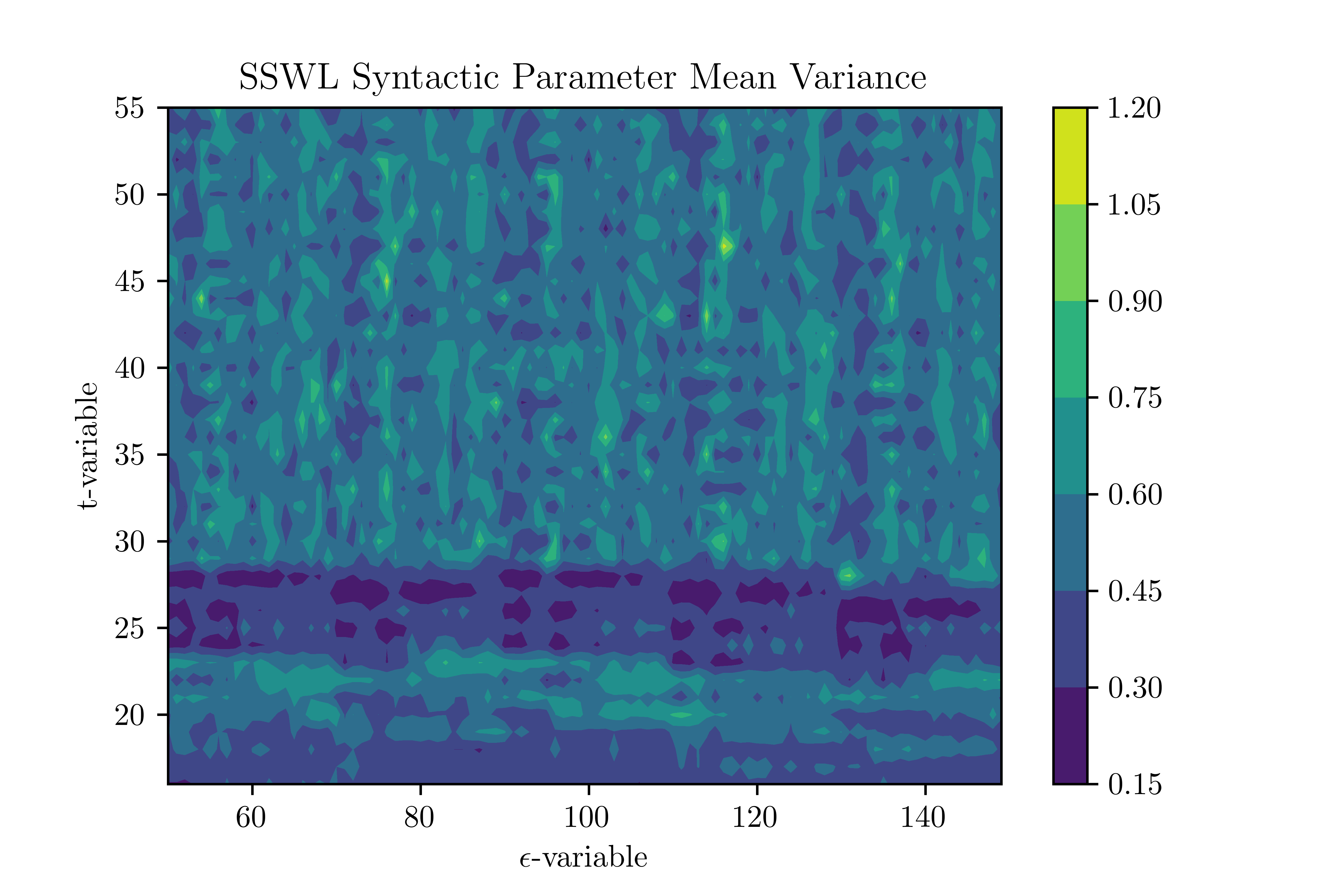
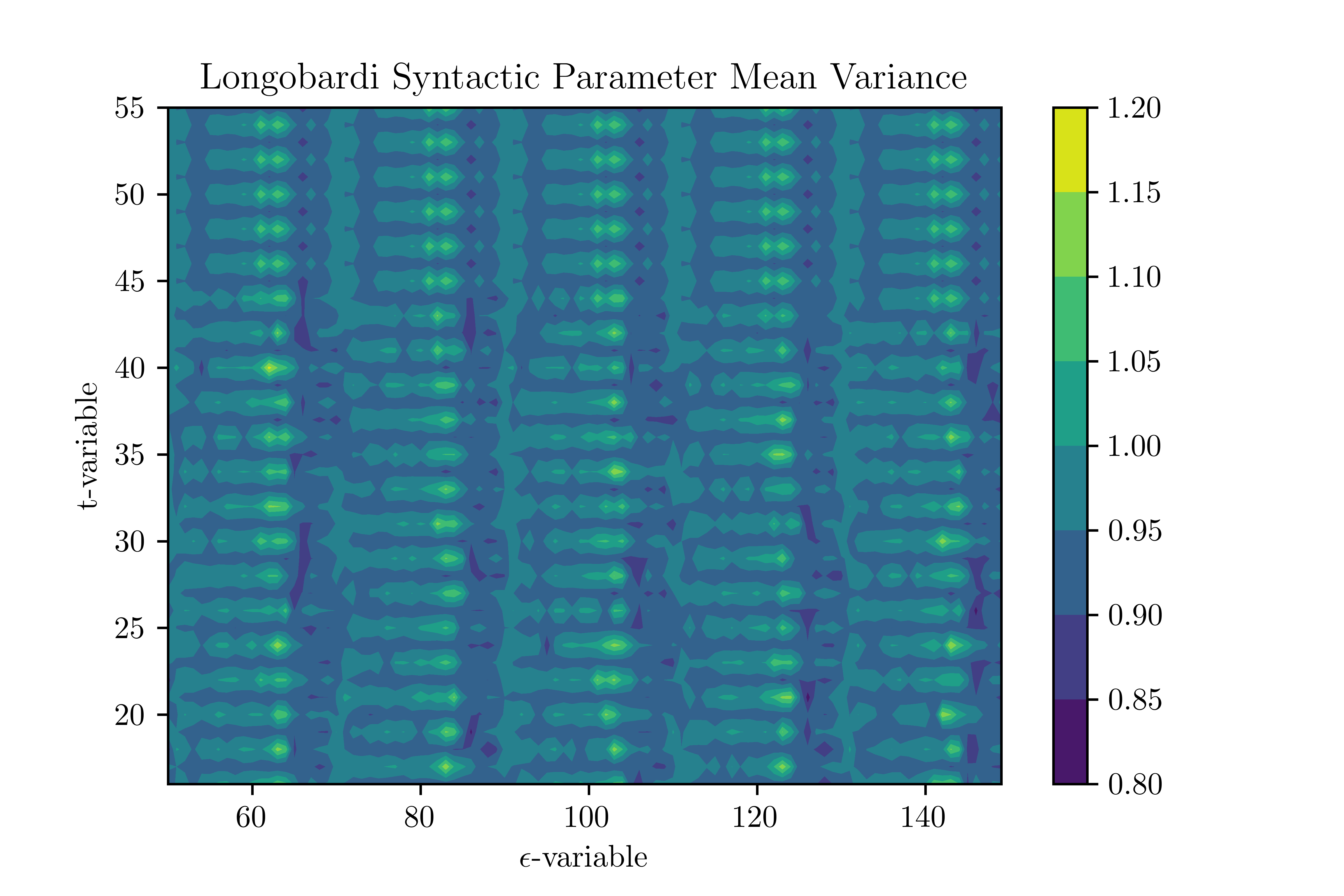
Figure 12. Contour plots of the variance of syntactic parameters as a function of the graph parameters $\epsilon$ and $t$. The yellow points indicate peaks in variance of the syntactic parameters.

The $\epsilon$-$t$ parameter space was explored to determine which values of $\epsilon$ and $t$ give rise to high variance in the distribution of each parameter under the mapping determined by the linear transformation $T$ of (2.3), (2.4) associated to a given weighted graph $G(\epsilon,t)$. The reason for considering this high variance condition is similar to the usual argument in the setting of principal component analysis, where high variance is used as an indicator that the resulting variables are highly independent. Thus, the high variance regions we identify in the $\epsilon$-$t$ space should be regarded as choices of the $\epsilon$-$t$ parameters that optimize the Belkin–Niyogi representation in the sense that the Laplace eigenfunction projections provide a set of highly independent variables for the representation of syntactic parameters. The resulting contour plot identifying high variance regions is shown in Figure 12.

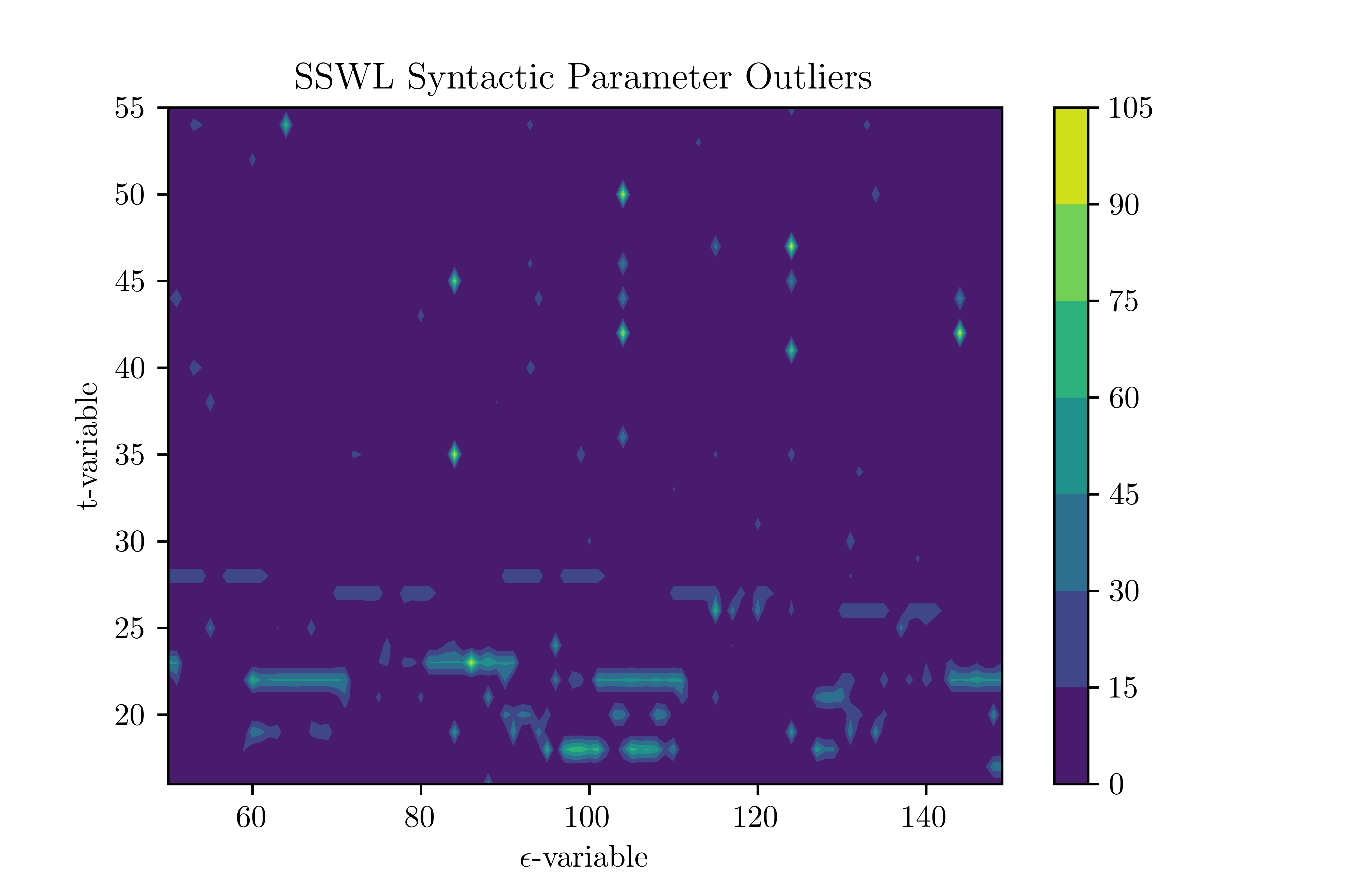
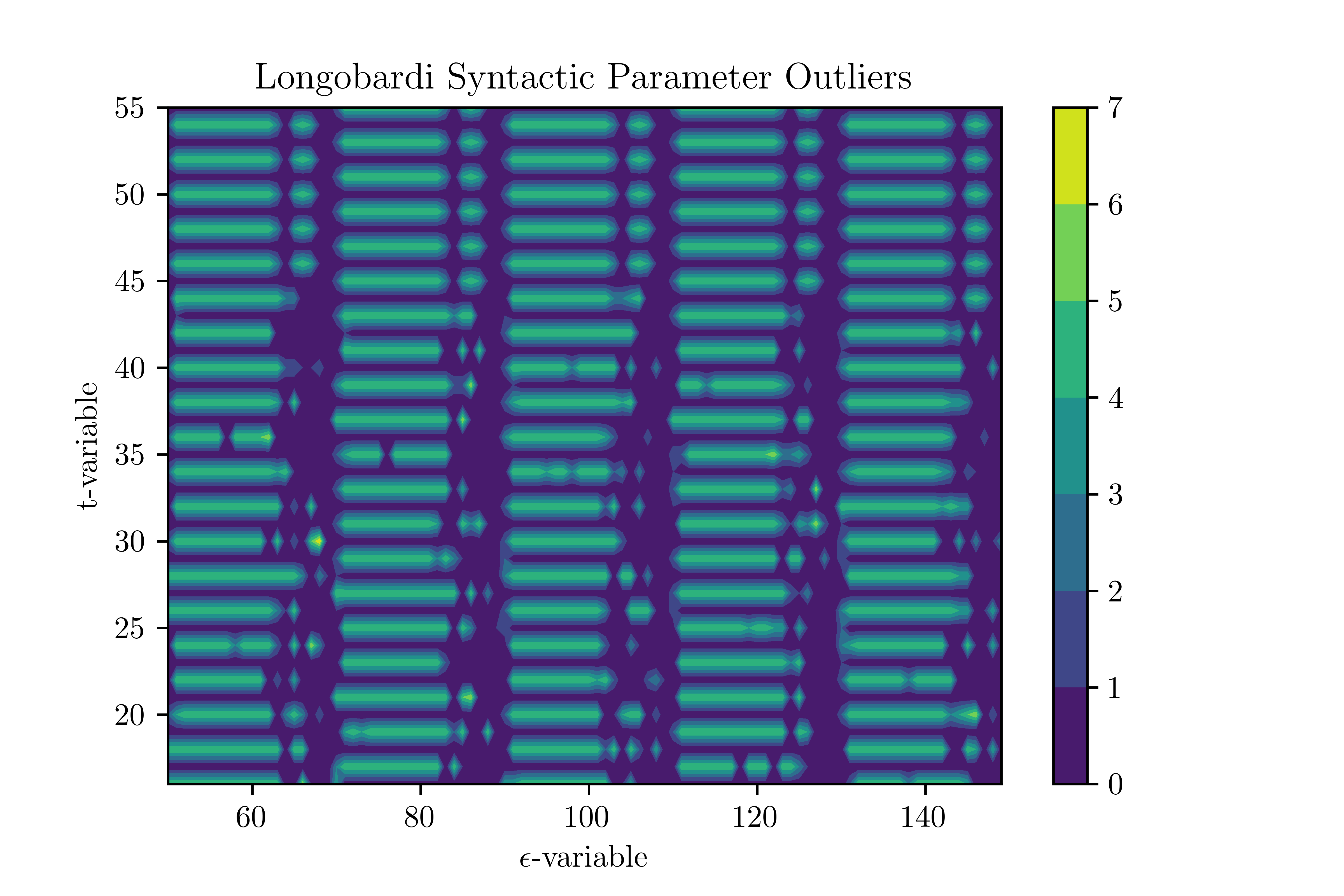
Figure 13. Contour plots of the number of outliers of syntactic parameters as a function of the graph parameters $\epsilon$ and $t$.

Another test aimed at identifying especially interesting regions in the $\epsilon$-$t$ space was conducted using a measure of the number of outliers produced among the set of coordinates for a given parameter. This measure indicated similar high magnitude in the regions analyzed with the previous method.

Let ${\mathcal{L}}$ be the set of languages in the database under consideration. We regard each $\ell_{i}\in{\mathcal{L}}$ as a binary vector $\ell_{i}\in{\mathbb{F}}_{2}^{n}$, where $n$ is the total number of syntactic parameters in the database, $\ell_{i}=(p_{i,j})_{j=1}^{n}$, where $p_{i,j}$ is the value that the $j$-th parameter takes in the $i$-th language. Similarly, we view each parameter $p_{j}$ as a vector $p_{j}\in{\mathbb{F}}_{2}^{N}$, where $N=\#{\mathcal{L}}$ is the number of languages in the database, $p_{j}=(p_{i,j})_{i=1}^{N}$.

Counting the number of outliers of the set $p_{j}=\{p_{i,j}\,|\,\ell_{i}\in{\mathcal{L}}\}$ and averaging that measure over all the sets of parameters gives a new measure of how the Laplacian eigenfunctions map method for dimensional reduction improves the efficiency of the new parameters to describe the languages in ${\mathcal{L}}$. The resulting plot of the number of outliers is given in Figure 13.

4.3. Clustering coefficients

We compute clustering coefficients of the nodes of the graphs $G(\epsilon,t)$ using the NetworkX package [12].

Consider an undirected graph $G_{i}=(V,E)$ composed of its set of vertices $V=V(G)$ (nodes) and set of edges $E=E(G)$, generated from a chosen region of the $\epsilon$-$t$ parameter space identified according to the analysis described in the previous subsections. The neighborhood, $\mathbb{V}_{i}$ of any given node, $v_{i}\in V(G)$ is the set of all nodes connected to that node. The size of $\mathbb{V}_{i}$ is referred to as the degree (valence) of the vertex $d_{i}=\deg(v_{i})=\#\mathbb{V}_{i}$. Since we are dealing with graphs that do not have parallel edges (are not multigraphs), the valence also counts the number of edges connected to $v_{i}$. The cardinality

(4.1) $$K_{i}=\#\{e\in E(G)\,|\,\partial(e)\cap\mathbb{V}_{i}\neq\emptyset\}$$

of the set all the edges connected to any of the vertices $v_{k}\in\mathbb{V}_{i}$ gives a measure of the clustering in the neighborhood of the vertex $v_{i}$. The local clustering coefficient $C_{i}$ of a vertex $v_{i}$ is then given by

(4.2) $$C_{i}=\frac{K_{i}}{{d_{i}\choose 2}}$$

Using the NetworkX package, the values $K_{i}$ can be determined from the graph objects present in the environment and the degrees $d_{i}$ are immediately available for any given node.

The variance of the clustering coefficients $C_{i}$ as a function of the $\epsilon$-variable in the $\epsilon$-neighborhood construction of the graph are well approximated by a Gaussian law of the form

$$f(x)=A\exp\left({-\frac{(x-H)^{2}}{\sigma^{2}}}\right)+V,$$

with the parameters as indicated in the Table, see Figure 14.

Fit Parameter	Value	1$\sigma$ Error ($\%$)
$A$	0.3359	0.3359
$H$	47.9530	22.99
$\sigma$	33.35	43.78
$V$	0.0541	0.002310

Table 1. SSWL Gaussian-Fit Parameter Data

Fit Parameter	Value	1$\sigma$ Error ($\%$)
$A$	0.4025	0.4070
$H$	18.2832	15.74
$\sigma$	18.5040	26.10
$V$	0.02934	0.1496

Table 2. Longobardi Gaussian-Fit Parameter Data

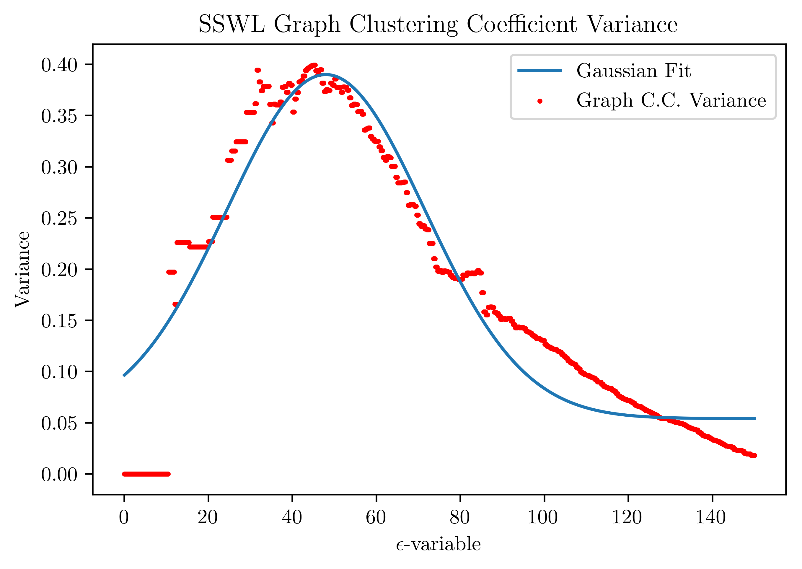
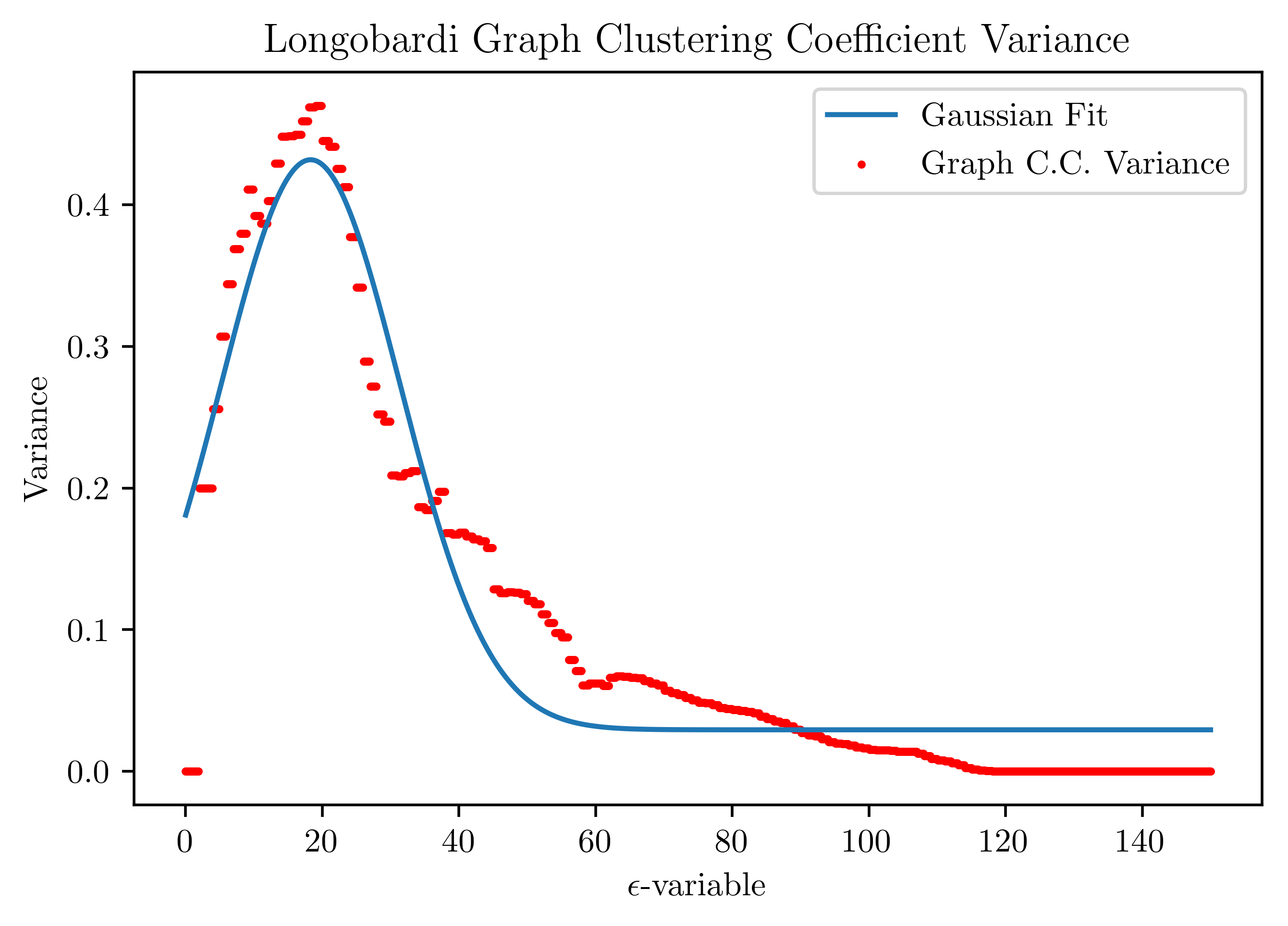
Figure 14. A plot of the variance among the clustering coefficents of a graph $G(\epsilon)$ as a function of $\epsilon$.

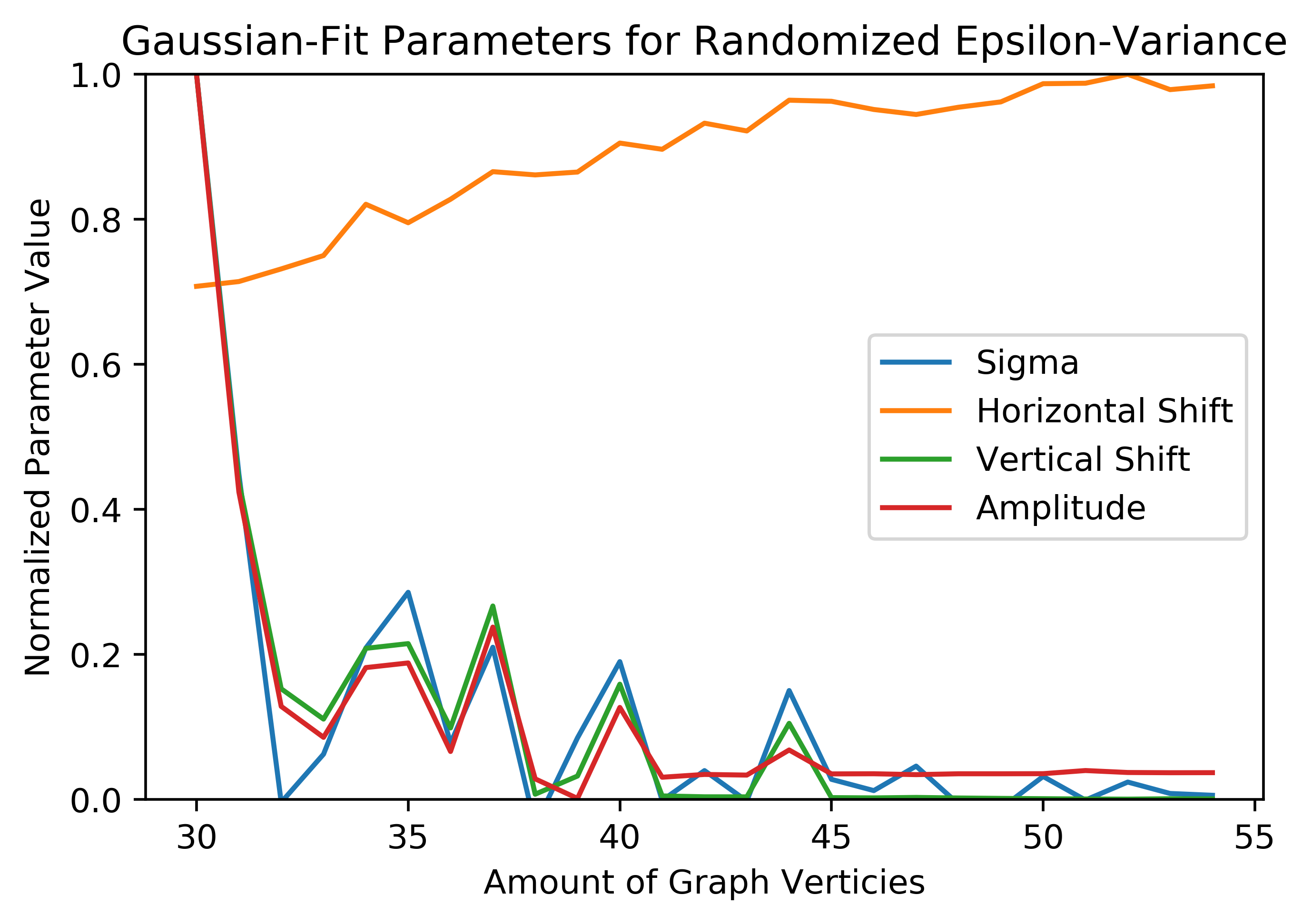
Figure 15. Gaussian parameters $\sigma$, $H$, $V$, and $A$ for random graphs as a function of the number of vertices.

We compare this behavior with that of random graphs with a varying number of vertices, obtained by generating random binary $n\times 260$ matrices where $n$ is the number of graphs vertices and using them as parameter data to generate graphs. A plot of the values of the Gaussian parameters $\sigma$, $H$, $V$, and $A$ as a function of the number of vertices in the graph is shown in Figure 15. The convergence of the horizontal shift $H$ indicates that this value only partially depends on the number of vertices in the graph and possibly on the number of parameter values at each vertex. The values of $\sigma$ and of the amplitude $A$ appear to converge to small but non-zero values, and the vertical shift value $V$ appears to converge to zero.

The set of all clustering coefficients $C_{i}$ can be used further in the context of phylogenetic reconstructions of language families, as outlined in the last section of [11]. Namely, the phylogenetic models used in [11] based on the method of phylogenetic algebraic geometry, are based on considering individual parameters as identically distributed independent random variables evolving according to the same Markov process on a tree. This hypothesis is not appropriate in view of the many relations that exist between syntactic parameters (some known explicitly, as those described in [8], [9]) and others only detected statistically, as discussed in the present paper, or with a different method in [10]. A modification of the phylogenetic model can be obtained by introducing different weights attached to different parameters in the boundary distribution at the leaves of the tree, which gives more weight in the model to parameters that are more likely to be “independent variables” and less weight to those that have a high degree of dependency on others. The latter can be measured in different possible ways, for instance through a degree of recoverability in Kanerva network as was done in [10], or through a function of the clustering coefficients computed here. We will return to investigate this kind of application in future work.

References

- [1] M. Baker, The Atoms of Language, Basic Books, 2001.
- [2] M. Belkin, P. Niyogi, Laplacian Eigenmaps and Spectral Techniques for Embedding and Clustering, in “Advances in Neural Information Processing Systems 14” pp.585–591, MIT Press, 2001.
- [3] M. Belkin, P. Niyogi, Laplacian eigenmaps for dimensionality reduction and data representation, Neural Comput. 15 (6) (2003) 1373–1396.
- [4] M. Belkin, P. Niyogi, Towards a theoretical foundation for Laplacian-based manifold methods, J. Comput. System Sci. 74 (2008), no. 8, 1289–1308.
- [5] N. Chomsky, Lectures on Government and Binding, Dordrecht, 1981.
- [6] N. Chomsky, H. Lasnik, The theory of Principles and Parameters, in “Syntax: An international handbook of contemporary research”, pp.506–569, de Gruyter, 1993.
- [7] Dimitar Kazakov, Guido Cordoni, Eyad Algahtani, Andrea Ceolin, Monica A. Irimia, Shin-Sook Kim, Dimitris Michelioudakis, Nina Radkevich, Cristina Guardiano, Giuseppe Longobardi, Learning Implicational Models of Universal Grammar Parameters, in “The Evolution of Language: Proceedings of the 12th International Conference (EVOLANGXII)”, 2017.
- [8] G. Longobardi, C. Guardiano, Evidence for syntax as a signal of historical relatedness, Lingua, 119 (2009) 1679–1706.
- [9] G. Longobardi, Principles, Parameters, and Schemata. A constructivist UG, Linguistic Analysis, 41 (2017) 3-4, 517–557.
- [10] J.J. Park, R. Boettcher, A. Zhao, A. Mun, K. Yuh, V. Kumar, M. Marcolli, Prevalence and recoverability of syntactic parameters in sparse distributed memories, in “Geometric Science of Information. Third International Conference GSI 2017”, pp. 265–272, Lecture Notes in Computer Science, Vol.10589, Springer 2017.
- [11] K. Shu, A. Ortegaray, R.C. Berwick, M. Marcolli, Phylogenetics of Indo-European language families via an algebro-geometric analysis of their syntactic structures, arXiv:1712.01719 [cs.CL]
- [12] NetworkX Software for Complex Networks, https://networkx.github.io/
- [13] Syntactic Structures of World Languages (SSWL) http://sswl.railsplayground.net/