Vibrational properties of metastable polymorph structures by machine learning

Abstract

Despite vibrational properties being critical for the ab initio prediction of the finite temperature stability and transport properties of solids, their inclusion in ab initio materials repositories has been hindered by expensive computational requirements. Here we tackle the challenge, by showing that a good estimation of force constants and vibrational properties can be quickly achieved from the knowledge of atomic equilibrium positions using machine learning. A random-forest algorithm trained on only 121 metastable structures of KZnF₃ reaches a maximum absolute error of 0.17 eV/$\textrm{\AA}^{2}$ for the interatomic force constants, and it is much less expensive than training the complete force field for such compound. The predicted force constants are then used to estimate phonon spectral features, heat capacities, vibrational entropies, and vibrational free energies, which compare well with the ab initio ones. The approach can be used for the rapid estimation of stability at finite temperatures.

Introduction

Large databases of calculated material properties, such as AFLOW.org^{1, 2}, the Materials Project³, and OQMD⁴, have become powerful tools for accelerated materials design^{5, 6, 7}. Ab initio relaxed crystal structures and ground state energies are routinely provided in these repositories, and often used to evaluate phase diagrams starting from zero temperature or with simple approximations ⁸. With this approach roughly 50% of the experimentally known compounds are found above the convex hull.^{9, 10} This can be due to the experimental structure being truly metastable. Another possible explanation could be the lack of accuracy of standard density functional approximations.¹¹ However, an important factor will undoubtedly be that phonon-related contributions are highly important at the temperatures of interest^{12, 13, 14, 15, 16}. These contributions are often neglected, principally due to the high computational cost posed by the interatomic force constants (IFC) matrix, i.e.the Hessian, or second derivatives of the energy with respect to the atomic displacements. Similarly, structural global energy minimization methods, such as USPEX^{17, 18}, generate hundreds of relaxed candidate structures. However, both for large databases and global energy methods, the vibrational energy contributions are typically too expensive to be calculated with brute force. A considerable advantage would come from an on-the-fly estimation of vibrational free energies during the search.

Neglecting phonon contributions to the free energy is obviously wrong and this practice is mainly due to computational necessities. Obtaining the Hessian typically requires one or two orders of magnitude more computer time than the corresponding structural relaxation. However, neglecting phonons can have dramatic consequences. For example, vibrational contributions have been shown to modify the sequence of reactions occurring as a function of temperature or pressure¹⁴, to explain the precipitation sequence of metallurgical phases¹⁹, or to alter the stability ordering of novel 2D material phases¹⁵. Phonons also have been shown to be as important as configurational disorder for the prediction of alloy phase diagrams and thereby essential to obtain experimental agreement^{12, 13}. Particularly relevant is the problem of polymorphs, i.e. materials sharing the same chemical composition but having different crystal structures. Calculations on organic molecules have shown that $\sim$69% of polymorph pairs reversed their relative stability when increasing the temperature, due to the vibrational contribution to the free energy²⁰. Also, roughly 50% of the compounds in the Materials Project database are metastable with a median energy above the convex hull of 15 meV/atom¹⁰ and similar values apply to the ICSD ²¹ repository within AFLOW.org. This energy is comparable to typical phonon free energy differences between polymorphs^{22, 19, 23}, highlighting the importance of including the phonon vibrational energy when determining the finite temperature ground states. The high-throughput prediction of phase diagrams at finite temperatures is still a major challenge for computational materials design, mostly because of the difficulty to quickly compute Hessians ^{6, 7}. Clearly, there is an urgent need for a rapid and reliable approach to predict the IFCs.

Machine learning (ML) algorithms can be used to avoid costly calculations. ML has been successfully used to predict IFCs for compounds from the same crystal structure but different chemical composition ^{24, 25}, which was subsequently shown to be a major factor determining the vibrational free energy of compounds²⁶. However, the more complex problem of predicting IFCs of competing structures of the same composition has not been addressed. Often the relaxed structures are already known and the challenge is to predict only the computationally expensive Hessians. This is the case with large ab initio databases, which contain many metastable structures or artificial configurations for sampling the phase space ². Contrary to force-field fitting where a continuum of “deformations$\rightarrow$forces” states has to be sampled, here accurate representations of the potential energy surface around diverse and potentially uncorrelated metastable states is needed. Is this doable? In the present work we tackle the challenge by finding an efficient solution with the help of random forests, trained with only one hundred metastable structures, but still capable of predicting accurate IFCs, spectral properties and thermodynamic quantities.

Approach

The interatomic force constants between atom $i$ and $j$ constitute a second-order tensor defined by the second derivatives of the PES with respect to atomic displacements

$$\mathbf{\Phi}_{ij}=(\nabla_{\!\mathbf{r}_{i}}\otimes\nabla_{\!\mathbf{r}_{j}})E$$ (1)

For ML to predict the $\mathbf{\Phi}_{ij}$’s we need to construct atom-centered descriptors based on an internal coordinate representation that is invariant with respect to the symmetries of the systems, as well as permutations among atoms of the same species. A similar challenge is faced in force-field fitting^{27, 28, 29} but here we face the additional problem of generalizing the concept to tensors.

Scalar quantities of the physical system, like the energy, are expressed in this representation as functions of a set of scalar descriptors, $\{g_{i,j}^{\alpha}\}$, based on these internal coordinates. Vector quantities associated to the $i^{\textrm{th}}$-atom can similarly be expressed by descriptors $g_{ij}^{\alpha}\mathbf{r}_{ij}$, that transform contravariantly. More generally, however, one can produce quantities that transform as tensors by taking gradients of the scalar descriptors.

We choose a series of Gaussians, similar to those used in force-field fitting²⁷, to represent the pair part

$$g_{ij}^{\alpha}=e^{-\left({\mathbf{r}_{ij}\over a_{\alpha}}\right)^{2}}$$ (2)

where $\left\{a_{\alpha}\right\}$ are a set of radii spanning a few interatomic distances encompassing atoms $i$ and $j$. Taking the gradients of these scalar descriptors leads to $3\times 3$ matrices defined for each atomic pair $(i,j)$ as:

$$M^{\eta,\eta^{\prime}}\equiv{\partial^{2}\over\partial{x_{i}}^{\eta}\partial{x_{j}}^{\eta^{\prime}}}g_{ij}^{\alpha}={2\over a_{\alpha}^{2}}g_{ij}^{\alpha}\left[\delta^{\eta,\eta^{\prime}}-{{2r^{\eta}_{ij}r^{\eta^{\prime}}_{ji}}\over{a_{\alpha}^{2}}}\right],$$ (3)

where $\eta$ and $\eta^{\prime}$ run over the three Cartesian coordinates. While the $\delta$ term transforms as a scalar, the $r_{ij}^{\eta}r_{ji}^{\eta^{\prime}}$ term corresponds to the outer product of the gradients of scalar function $g$ and transforms as a rank-2 tensor. Therefore, descriptors of the type

$$\mathbf{D}_{ij}^{(2)\alpha}=(\nabla_{\!\mathbf{r}_{i}}\otimes\nabla_{\!\mathbf{r}_{j}})g_{ij}^{\alpha}\propto g_{ij}^{\alpha}\mathbf{r}_{ij}\otimes\mathbf{r}_{ji},$$ (4)

transform as rank-2 tensors and can be used for the regression of Hessians. Periodic boundary conditions within the supercell spanning the force cut-off range (here $5\times 5\times 5$) require an extra modification of the descriptor as

$${\mathbf{D}}_{i,j}^{(2)\alpha}=\sum_{m}e^{-\left|{\mathbf{r}_{ij}+\mathbf{R}_{m}\over a_{\alpha}}\right|^{2}}(\mathbf{r}_{ij}+\mathbf{R}_{m})\otimes(\mathbf{r}_{ji}-\mathbf{R}_{m}),$$ (5)

where $\mathbf{R}_{m}$ are the translation vectors connecting identical atoms in the supercell.

The set of descriptors above can be extended to higher orders, at an increased computational expense. For instance, the following set of rank-2 tensor descriptors would capture further 3-body interactions.

$${\mathbf{D}}_{ij}^{(3)\alpha,\beta,\gamma} = \sum_{k}\{g_{ik}^{\alpha}g_{kj}^{\beta}\nabla_{\!\mathbf{r}_{i}}\theta_{ikj}\otimes\nabla_{\!\mathbf{r}_{j}}\theta_{ikj}+g_{ij}^{\gamma}g_{jk}^{\beta}\nabla_{\!\mathbf{r}_{i}}\theta_{ijk}\otimes\nabla_{\!\mathbf{r}_{j}}\theta_{ijk}+g_{ki}^{\alpha}g_{ij}^{\gamma}\nabla_{\!\mathbf{r}_{i}}\theta_{kij}\otimes\nabla_{\!\mathbf{r}_{j}}\theta_{kij}\}$$ (6)

$$\equiv \sum_{k}{\mathbf{D}}^{\alpha,\beta,\gamma}_{i,k,j}.$$

where $\theta_{ijk}$ is the angle formed by atoms $i$,$j$ and $k$. The gradients of $\theta_{ijk}$ can be expressed in terms of cross products of pairs in $\{i,j,k\}$ and ${\mathbf{D}}_{ij}^{(3)}$ transform as a tensor. There are other ways to define descriptors involving two and three-atom terms^{27, 30}. However, to the best of our knowledge, direct regression of Hessians using invariant tensorial-form descriptors has not been attempted before.

Descriptors $D_{i,j}^{(2)\alpha}$ are used to predict $\mathbf{\Phi}_{ij}$, i.e. the $3\times 3$ matrices of IFCs between different $i$- and $j$-atoms. Atomic force constants of the form, $\mathbf{\Phi}_{ii}$, which simply describes the forces on atom $i$ due to its own displacement, cannot come from $D_{i,i}^{(2)\alpha}$. Thus, the whole environment is included through the sum:

$${\mathbf{D}}_{i,i}^{({\mathrm{diag}})(2)\alpha}=\sum_{j}{\mathbf{D}}_{i,j}^{(2)\alpha},$$ (7)

where $j$ indices through all the atoms of the supercell , including $i$ itself. To get the whole IFCs, two different ML models are then trained: $D_{i,j}^{(2)\alpha}\xRightarrow{\text{\footnotesize ML}}\mathbf{\Phi}_{i\neq j}$ and $D_{i,i}^{({\mathrm{diag}})(2)\alpha}\xRightarrow{\text{\footnotesize ML}}\mathbf{\Phi}_{ii}$.

For clarity of the presentation, the dependence on chemical species, required for multi-component systems, has not been included in previous the formulas. Given a set of species $\{s\}$, the descriptors can be written as ${\mathbf{D}}_{s,s^{\prime};i,j}^{(2)\alpha}\equiv(\delta_{s_{i},s}\delta_{s_{j},s^{\prime}}+\delta_{s_{i},s^{\prime}}\delta_{s_{j},s}){\mathbf{D}}_{i,j}^{(2)\alpha}$, and ${\mathbf{D}}^{(3)\alpha,\beta,\gamma}_{s,s^{\prime},s^{\prime\prime},i,j}=\sum_{k}\delta_{s_{k},s^{\prime\prime}}(\delta_{s_{i},s}\delta_{s_{j},s^{\prime}}+\delta_{s_{i},s^{\prime}}\delta_{s_{j},s}){\mathbf{D}}^{(3)\alpha,\beta,\gamma}_{i,j,k}$, with $s$ and $s^{\prime}$ species indices.

Results and discussion

Data set.

The ML approach is developed for a test chemical system: the metastable structures of KZnF₃ (a cubic perovskite at 0K, chosen for simplicity). The initial data set consists of 267 KZnF₃ structures with 10 atoms per unit cell, randomly generated by the first-generation run of the USPEX code^{17, 18}, and optimized using density functional theory (DFT)^{31, 32} as implemented in VASP ³³. The projector augmented wave (PAW) method is employed to deal with the core and valence electrons³⁴. The data sets preparation follows AFLOW.org high-throughput recommendations ^{1, 35, 36}, and the kinetic energy cutoffs are set to 450 eV for the plane wave basis. The force constant matrices and the phonon frequencies are computed at $\Gamma$ using density functional perturbation theory³⁷.

The identification and reduction of symmetrically equivalent cells is performed through the following structural fingerprint. For every structure $C$, descriptors are computed for each $i$-, $j$-atom pair: $D_{s,s^{\prime};i,j}(C)^{\alpha}\equiv(\delta_{s_{i},s}\delta_{s_{j},s^{\prime}}+\delta_{s_{i},s^{\prime}}\delta_{s_{j},s})g_{ij}^{\alpha}(C)$, where $\{s,s^{\prime}\}$ are the species indices (these same descriptors are also employed to predict the IFC matrix invariants, as detailed later). The sum over the pairs leades to a fingerprint $K$ for a given structure $C$:

$$K^{\alpha}_{s,s^{\prime}}(C)\equiv\sum_{i,j}D_{s,s^{\prime};i,j}^{\alpha}(C)=\sum_{i,j}(\delta_{s_{i},s}\delta_{s_{j},s^{\prime}}+\delta_{s_{i},s^{\prime}}\delta_{s_{j},s})g_{ij}^{\alpha}(C)$$ (8)

The distance $d(C_{1},C_{2})$ between structures $C_{1}$ and $C_{2}$ is then defined as:

$$d(C_{1},C_{2})\equiv\sum_{(s,s^{\prime};\alpha)}\frac{|K^{\alpha}_{s,s^{\prime}}(C_{1})-K^{\alpha}_{s,s^{\prime}}(C_{2})|}{|K^{\alpha}_{s,s^{\prime}}(C_{1})|+|K^{\alpha}_{s,s^{\prime}}(C_{2})|}.$$ (9)

After combinatorial analysis between the structures, an optimum distance’s threshold of 0.35 is found by inspection. Only 121 inequivalent configurations are found, the remaining ones being discarded as duplicates (Supplementary Materials). The 121 cells are then used to build the ML model and assess its performance.

Predicting force constants.

Amongst the available regression algorithms, random forests (RF) are chosen because they are non-parametric, require virtually no data pre-conditioning, and usually yield robust and reliable results. The scikit-learn implementation³⁸ is used to assess the performance of the model via 10-fold cross validation. The forest contain 100 trees: better performance was not noticed with larger forests. The three independent scalar invariants ³⁹ $\{tr(\mathbf{\Phi}_{ij}),\sqrt{tr(\mathbf{\Phi}_{ij}^{2})},\sqrt[3]{tr(\mathbf{\Phi}_{ij}^{3})}\}$ — derived from calculated or predicted Hessians and defined for each IFC between different atoms — are used to assess the quality of the model. The performance of the random forests is listed in Table 1 and depicted in Figure 1.

Table 1: Performance: statistical analysis of DFT calculations versus RFs predictions.

	Pearson	Spearman	mean absolute	root mean
	coefficient	coefficient	error	square error
$tr(\mathbf{\Phi}_{ij})$	0.99	0.98	0.25	0.38
			(eV/$\textrm{\AA}^{2}$)	(eV/$\textrm{\AA}^{2}$)
$\sqrt{tr(\mathbf{\Phi}_{ij}^{2})}$	0.98	0.95	0.27	0.41
			(eV/$\textrm{\AA}^{2}$)	(eV/$\textrm{\AA}^{2}$)
$\sqrt[3]{tr(\mathbf{\Phi}_{ij}^{3})}$	0.98	0.95	0.28	0.43
			(eV/$\textrm{\AA}^{2}$)	(eV/$\textrm{\AA}^{2}$)
$\mathbf{\Phi}_{ij}$	0.99	0.93	0.17	0.32
			(eV/$\textrm{\AA}^{2}$)	(eV/$\textrm{\AA}^{2}$)
variance	0.88	0.87	0.88	1.14
$\sqrt{\overline{\left(\omega-\overline{\omega}\right)^{2}}}$			(rad/ps)	(rad/ps)
mean	0.92	0.88	0.73	0.94
$\overline{\omega}$			(rad/ps)	(rad/ps)
max	0.88	0.87	3.79	4.63
$\omega_{\begin{subarray}{c}\scalebox{0.6}{max}\end{subarray}}$			(rad/ps)	(rad/ps)
$C_{v}$	0.91	0.83	0.0008	0.0010
			(meV/K/atom)	(meV/K/atom)
$F_{\begin{subarray}{c}\scalebox{0.6}{vib}\end{subarray}}$	0.82	0.80	2.92	3.78
			(meV/atom)	(meV/atom)
$S_{\begin{subarray}{c}\scalebox{0.6}{vib}\end{subarray}}$	0.80	0.79	0.009	0.012
			(meV/K/atom)	(meV/K/atom)

Upon trying with various different choices of radii $a_{\alpha}$, the best results are achieved with $a_{\alpha}=\{1,2,3,...,30\}$ Å. The outcome of the descriptor with periodicity (Eq. (5)) is satisfactory. On the contrary, the performance is poor when periodicity is neglected (mean absolute errors are larger than 1eV/$\textrm{\AA}^{2}$, see Supplementary Materials). Errors are larger on small supercells, and decrease if training is performed on larger systems.

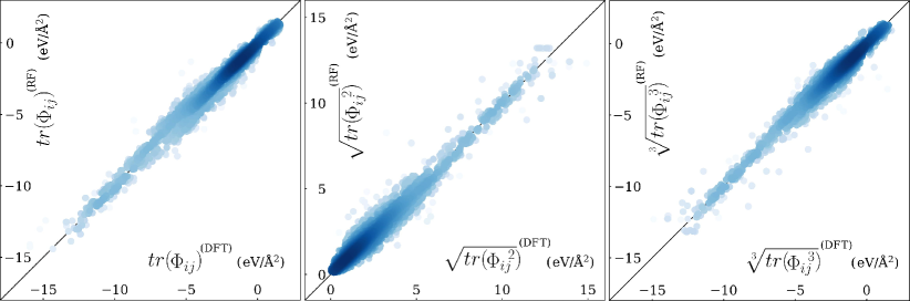
Figure 1: Random forest performance: predictions versus calculations of force constant sub-matrix components across $i$- and $j$-atoms. The abscissa shows the values obtained with DFT, and the ordinate those obtained with RFs.

The full Hessian is tackled with the descriptors from Eq. (5) and Eq. (7). The individual force constants predicted versus calculated — are compared in Figure 2 and listed in Table 1.

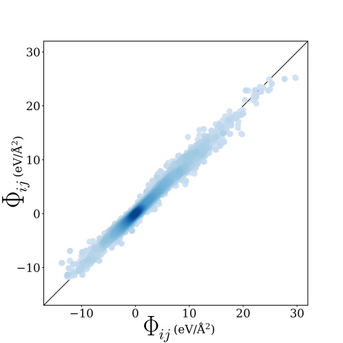
Figure 2: Random forest performance: predictions versus calculations for individual interatomic force constants. The abscissa shows the values computed with DFT and the ordinate shows the values obtained with RFs.

The RF results indicate that very good predictions can be obtained using only simple two-atom descriptors. The extension to the 3-atom environments, Eq. 6, does not noticeably improve the outcome, implying that the key factors determining the IFCs are the species and relative positions between atoms’ pairs, without much contribution from other environmental atoms. 3-atom descriptors take much longer to calculate, are much more numerous than the pair descriptors, and therefore impose constraints onto the number of accessible radii $\{\alpha\}$, potentially leading to sub optimal results. Thus, it is possible that other descriptor algebraic formalisms and/or broader training sets – more systems and larger structures — could improve the outcome when 3-atom environments are accessed. This is beyond the scope of the current work and it will be tackled in the future.

How does the promising accuracy of predicted IFCs translate into vibrational properties? Errors do accumulate and even an apparently good prediction of forces could still violate conservation rules of the system leading to unphysical results. The phonon frequencies of the different KZnF₃ cells are computed from the RF-predicted IFCs. Results are extremely sensitive to small inaccuracies in predicted forces and imaginary phonon frequencies appear.

The imaginary modes are removed by correcting each Hessian $H$ to the “closest” semipositive definite matrix $H^{\prime}$. A diagonal matrix $D$ is obtained through the basis transformation $H=PDP^{T}$. A corrected $D\rightarrow D_{\rm c}$ is produced by replacing the negative terms with zeroes. The object is rotated back to the original basis, $PD_{\rm c}P^{T}$. The term is further corrected by enforcing the acoustic sum rule leading to $H_{\rm c}=(I-Q)(PD_{\rm c}P^{T})(I-Q)$, with $Q\equiv\sum_{t=1,2,3}v_{t}^{T}v_{t}$, $v_{t}$ a vector of size $3N_{\begin{subarray}{c}\scalebox{0.6}{atoms}\end{subarray}}$ defined as $v_{t,i}={\delta_{i,k}}/{\sqrt{N_{\begin{subarray}{c}\scalebox{0.6}{atoms}\end{subarray}}}}$, and $k\equiv\left[(t-1)\mod 3\right]$.

The phonon frequencies are computed at $\Gamma$ from the corrected Hessian $H_{\rm c}$. Following Ref.  26, the zero frequencies are replaced by $\left<\omega_{\begin{subarray}{c}\scalebox{0.6}{opt}\end{subarray}}\right>/2$ ($\omega_{\begin{subarray}{c}\scalebox{0.6}{opt}\end{subarray}}$ represent the optical frequencies) in the calculation of vibrational properties. From here, phonon spectral distribution (mean, max, and variance) and thermodynamic properties are then obtained.

Figure 3 displays the square root of the variance, the mean, and the maximum of the compound frequencies, computed with DFT and predicted with RFs. There is good correlation and the statistical analysis is summarized in Table 1.

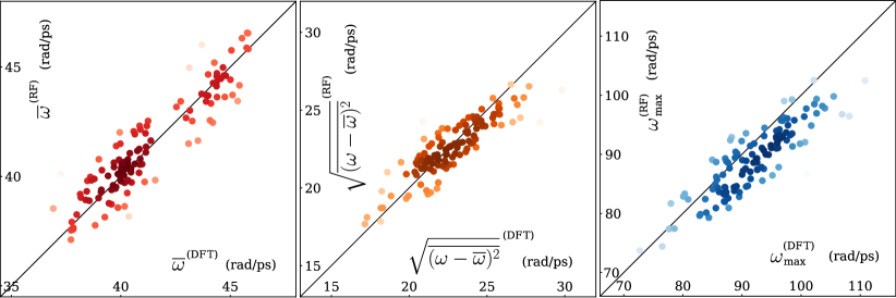
Figure 3: Plots of the square root of the variance (middle), the mean (left), and the maximum (right) of the compound frequencies. The $x$-axis shows the values computed with DFT and the $y$-axis shows the values obtained with RFs.

The specific heats at constant volume, vibrational entropies and free energies are computed at 300 K from the phonon frequencies $\omega$ following Ref. 40 ($N_{\mathrm{atoms}}$ is the number of atoms in the cell and $n_{\omega}$ is the Bose-Einstein distribution):

$$C_{\begin{subarray}{c}\scalebox{0.6}{V}\end{subarray}} = \frac{1}{N_{\mathrm{atoms}}}\sum_{\omega}\frac{\hbar^{2}\omega^{2}}{k_{\mathrm{B}}T^{2}}\frac{\exp\left(\frac{-\hbar\omega}{k_{\mathrm{B}}T}\right)}{\left(1-\exp\left(\frac{-\hbar\omega}{k_{\mathrm{B}}T}\right)\right)^{2}}$$

$$S_{\begin{subarray}{c}\scalebox{0.6}{vib}\end{subarray}} = \frac{1}{N_{\mathrm{atoms}}}\sum_{\omega}\left\{\frac{\frac{\hbar\omega}{T}\exp\left(\frac{-\hbar\omega}{k_{\mathrm{B}}T}\right)}{1-\exp\left\{\frac{-\hbar\omega}{k_{\mathrm{B}}T}\right)}-k_{\mathrm{B}}\ln{\left[1-\exp\left(\frac{-\hbar\omega}{k_{\mathrm{B}}T}\right)\right]}\right\}$$

$$F_{\begin{subarray}{c}\scalebox{0.6}{vib}\end{subarray}} = E_{\begin{subarray}{c}\scalebox{0.6}{vib}\end{subarray}}-TS_{\begin{subarray}{c}\scalebox{0.6}{vib}\end{subarray}}=-\frac{1}{N_{\mathrm{atoms}}}\sum_{\omega}\left(\frac{\hbar\omega}{2}+k_{\mathrm{B}}T\ln{n_{\omega}}\right)$$

The quantities are depicted in Figure 4: values computed with DFT are on the $x$-axis while values predicted with RFs are on the $y$-axis. The plots show that the RF approach gives a good approximation of the heat capacities, vibrational free energies and vibrational entropies of the different structures of KZnF₃. The statistical analysis is summarized in Table 1.

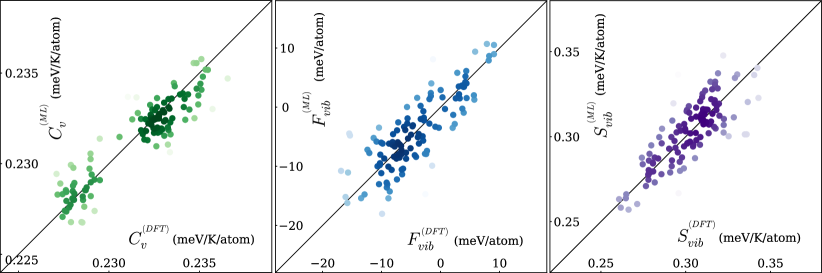
Figure 4: Heat capacities ($C_{\rm v}$), vibrational free energies ($F_{\rm vib}$), and vibrational entropies ($S_{\rm vib}$) are computed at 300 K with DFT and RFs.

The results illustrate that descriptors transforming as two-index tensors, in combination with RFs regression algorithms and relatively small training sets, can be used to predict IFCs for generic metastable crystal structures. Other approaches can be used to further improve the outcome: amongst them there are support vector machines or neural networks as algorithms, different descriptor definitions, inhomogeneous or adjustable grids for the radii, replacing the Gaussian by different functions, considering the species as separate descriptors from the structural ones. In addition, training on more and larger supercells, could improve the accuracy and enhance the relevance of 3-atom environmental descriptors, which could also take a different functional form from the presented one. However, regardless of potential improvements, here it has been shown that it is possible to predict force constants by training exclusively on metastable structures — very abundant in online respositories — without the necessity to include unstable configurations. Atomic configurations can be viewed as points in a high-dimensional space of rototranslation-permutation invariant descriptors: close points $\rightarrow$ similar properties. As such, to overcome similarity ML force fields are typically trained on tens of thousands of atomic configurations not corresponding to local energy minima, in order to have a sufficiently dense coverage of the representative hyper-volume in the configuration space: any new configuration is close to some other points in the training set, allowing for a good prediction of the energy/forces. In contrast, our case deals only with atomic configurations corresponding to local energy minima: metastable structures are intrinsically dissimilar, belonging to attraction basins separated by energy barriers in the configurational space. A priori there is no reason why the properties of such different structures should be related to each other. A posteriori, the results show that the Hessians of different local minima are indeed inter-related and strongly determined by pair-wise interactions. This unveils an underlying regularity in the character of the inter-atomic interactions that persists across the different metastable structures, enabling the prediction of force constants of an unknown metastable structure by training only on the other metastable systems available, without having to include any unstable structures to populate the empty configurational space between energy minima. The property can be leveraged for the quick estimation of vibrational contributions to phase stability and transport properties of materials, and to enable the high-throughput ab initio screening of these properties at finite temperatures.

Conclusions

We have shown that Hessians and associated vibrational properties of multi-component metastable structures can be efficiently predicted by machine learning regressions without the need of developing full force fields. The key factors determining the interatomic force constants are captured by tensor descriptors depending only on the species and distance between atoms’ pairs. The main features of the vibrational spectrum — maximum, mean and variance — are correctly reproduced. ML predictions of thermodynamic properties — specific heat, vibrational free energy and entropy — correlate well with the DFT calculations. Once trained, the model allows for the rapid vibrational characterization of relaxed structures with arbitrary complexity at low computational cost and the efficient comparison of polymorphs competing for stability at finite temperature. It is envisioned that machine learning vibrational-approaches will enable the use of the abundant online repositories information for efficient high-throughput screening of stability and transport at finite temperature.

References

- Curtarolo et al. 2012 Curtarolo, S.; Setyawan, W.; Hart, G. L. W.; Jahnátek, M.; Chepulskii, R. V.; Taylor, R. H.; Wang, S.; Xue, J.; Yang, K.; Levy, O.; Mehl, M. J.; Stokes, H. T.; Demchenko, D. O.; Morgan, D. AFLOW: An automatic framework for high-throughput materials discovery. Comput. Mater. Sci. 2012, 58, 218–226
- Curtarolo et al. 2012 Curtarolo, S.; Setyawan, W.; Wang, S.; Xue, J.; Yang, K.; Taylor, R. H.; Nelson, L. J.; Hart, G. L. W.; Sanvito, S.; Buongiorno Nardelli, M.; Mingo, N.; Levy, O. AFLOWLIB.ORG: A distributed materials properties repository from high-throughput ab initio calculations. Comput. Mater. Sci. 2012, 58, 227–235
- Jain et al. 2013 Jain, A.; Ong, S. P.; Hautier, G.; Chen, W.; Richards, W. D.; Dacek, S.; Cholia, S.; Gunter, D.; Skinner, D.; Ceder, G.; Persson, K. a. The Materials Project: A materials genome approach to accelerating materials innovation. APL Materials 2013, 1, 011002
- Kirklin et al. 2015 Kirklin, S.; Saal, J. E.; Meredig, B.; Thompson, A.; Doak, J. W.; Aykol, M.; Rühl, S.; Wolverton, C. The Open Quantum Materials Database (OQMD): assessing the accuracy of DFT formation energies. Npj Computational Materials 2015, 1, 15010
- Nosengo 2016 Nosengo, N. Can artificial intelligence create the next wonder material? Nature 2016, 533, 22–25
- Curtarolo et al. 2013 Curtarolo, S.; Hart, G. L. W.; Nardelli, M. B.; Mingo, N.; Sanvito, S.; Levy, O. The High-Throughput Highway to Computational Materials Design. Nat. Mater. 2013, 12, 191–201
- Green et al. 2017 Green, M. L. et al. Fulfilling the promise of the materials genome initiative with high-throughput experimental methodologies. Applied Physics Reviews 2017, 4, 011105
- Toher et al. 2017 Toher, C.; Oses, C.; Plata, J. J.; Hicks, D.; Rose, F.; Levy, O.; de Jong, M.; Asta, M. D.; Fornari, M.; Buongiorno Nardelli, M.; Curtarolo, S. Combining the AFLOW GIBBS and Elastic Libraries to efficiently and robustly screen thermomechanical properties of solids. Phys. Rev. Mater. 2017, 1, 015401
- Opahle et al. 2013 Opahle, I.; Parma, A.; McEniry, E. J.; Drautz, R.; Madsen, G. K. H. High-throughput study of the structural stability and thermoelectric properties of transition metal silicides. New Journal of Physics 2013, 15, 105010
- Sun et al. 2016 Sun, W.; Dacek, S. T.; Ong, S. P.; Hautier, G.; Jain, A.; Richards, W. D.; Gamst, A. C.; Persson, K. A.; Ceder, G. The thermodynamic scale of inorganic crystalline metastability. Science Advances 2016, 2
- Sun et al. 2016 Sun, J.; Remsing, R. C.; Zhang, Y.; Sun, Z.; Ruzsinszky, A.; Peng, H.; Yang, Z.; Paul, A.; Waghmare, U.; Wu, X.; Klein, M. L.; Perdew, J. P. Accurate first-principles structures and energies of diversely bonded systems from an efficient density functional. Nature Chem. 2016, 8, 831–836
- Liu et al. 2017 Liu, Z. T. Y.; Burton, B. P.; Khare, S. V.; Gall, D. First-principles phase diagram calculations for the rocksalt-structure quasibinary systems TiN–ZrN, TiN–HfN and ZrN–HfN. Journal of Physics: Condensed Matter 2017, 29, 035401
- Burton and van de Walle 2006 Burton, B. P.; van de Walle, A. First-principles phase diagram calculations for the system NaCl–KCl: The role of excess vibrational entropy. Chemical Geology 2006, 225, 222–229
- R. Akbarzadeh et al. 2007 R. Akbarzadeh, A.; Ozoliņš, V.; Wolverton, C. First-Principles Determination of Multicomponent Hydride Phase Diagrams: Application to the Li-Mg-N-H System. Advanced Materials 2007, 19, 3233–3239
- Carrete et al. 2017 Carrete, J.; Gallego, L. J.; Mingo, N. Structural Complexity and Phonon Physics in 2D Arsenenes. The Journal of Physical Chemistry Letters 2017, 1375–1380
- Körmann et al. 2017 Körmann, F.; Ikeda, Y.; Grabowski, B.; Sluiter, M. H. F. Phonon broadening in high entropy alloys. npj Computational Materials 2017, 3, 36
- Oganov and Glass 2006 Oganov, A. R.; Glass, C. W. Crystal structure prediction using ab initio evolutionary techniques: Principles and applications. The Journal of Chemical Physics 2006, 124, 244704
- Glass et al. 2006 Glass, C. W.; Oganov, A. R.; Hansen, N. USPEX — Evolutionary crystal structure prediction. Computer Physics Communications 2006, 175, 713 – 720
- Wolverton and Ozoliņš 2001 Wolverton, C.; Ozoliņš, V. Entropically Favored Ordering: The Metallurgy of Al2Cu Revisited. Phys. Rev. Lett. 2001, 86, 5518
- Nyman and Day 2015 Nyman, J.; Day, G. M. Static and lattice vibrational energy differences between polymorphs. CrystEngComm 2015, 17, 5154–5165
- Bergerhoff et al. 1983 Bergerhoff, G.; Hundt, R.; Sievers, R.; Brown, I. D. The inorganic crystal structure data base. J. Chem. Inf. Comput. Sci. 1983, 23, 66–69
- van de Walle and Ceder 2002 van de Walle, A.; Ceder, G. The effect of lattice vibrations on substitutional alloy thermodynamics. Reviews of Modern Physics 2002, 74, 11–45
- Curtarolo et al. 2005 Curtarolo, S.; Morgan, D.; Ceder, G. Accuracy of ab initio methods in predicting the crystal structures of metals: A review of 80 binary alloys. Calphad 2005, 29, 163–211
- Carrete et al. 2014 Carrete, J.; Li, W.; Mingo, N.; Wang, S.; Curtarolo, S. Finding Unprecedentedly Low-Thermal-Conductivity Half-Heusler Semiconductors via High-Throughput Materials Modeling. Phys. Rev. X 2014, 4, 011019
- van Roekeghem et al. 2016 van Roekeghem, A.; Carrete, J.; Oses, C.; Curtarolo, S.; Mingo, N. High-Throughput Computation of Thermal Conductivity of High-Temperature Solid Phases: The Case of Oxide and Fluoride Perovskites. Phys. Rev. X 2016, 6, 041061
- Legrain et al. 2017 Legrain, F.; Carrete, J.; van Roekeghem, A.; Curtarolo, S.; Mingo, N. How Chemical Composition Alone Can Predict Vibrational Free Energies and Entropies of Solids. Chemistry of Materials 2017, 29, 6220–6227
- Behler 2011 Behler, J. Atom-centered symmetry functions for constructing high-dimensional neural network potentials. The Journal of Chemical Physics 2011, 134, 074106
- Botu and Ramprasad 2015 Botu, V.; Ramprasad, R. Learning scheme to predict atomic forces and accelerate materials simulations. Phys. Rev. B 2015, 92, 094306
- Botu and Ramprasad 2015 Botu, V.; Ramprasad, R. Adaptive machine learning framework to accelerate ab initio molecular dynamics. International Journal of Quantum Chemistry 2015, 115, 1074–1083
- Artrith et al. 2017 Artrith, N.; Urban, A.; Ceder, G. Efficient and accurate machine-learning interpolation of atomic energies in compositions with many species. Physical Review B 2017, 96, 014112
- Hohenberg and Kohn 1964 Hohenberg, P.; Kohn, W. Inhomogeneous Electron Gas. Phys. Rev. 1964, 136, B864–B871
- Kohn and Sham 1965 Kohn, W.; Sham, L. J. Self-Consistent Equations Including Exchange and Correlation Effects. Phys. Rev. 1965, 140, A1133–A1138
- Kresse and Furthmüller 1996 Kresse, G.; Furthmüller, J. Efficiency of Ab-Initio Total Energy Calculations for Metals and Semiconductors Using a Plane-Wave Basis Set. Comput. Mater. Sci. 1996, 6, 15 – 50
- Kresse and Joubert 1999 Kresse, G.; Joubert, D. From Ultrasoft Pseudopotentials to the Projector Augmented-Wave Method. Phys. Rev. B 1999, 59, 1758–1775
- Taylor et al. 2014 Taylor, R. H.; Rose, F.; Toher, C.; Levy, O.; Yang, K.; Buongiorno Nardelli, M.; Curtarolo, S. A RESTful API for exchanging materials data in the AFLOWLIB.org consortium. Comput. Mater. Sci. 2014, 93, 178–192
- Calderon et al. 2015 Calderon, C. E.; Plata, J. J.; Toher, C.; Oses, C.; Levy, O.; Fornari, M.; Natan, A.; Mehl, M. J.; Hart, G. L. W.; Buongiorno Nardelli, M.; Curtarolo, S. The AFLOW standard for high-throughput materials science calculations. Comput. Mater. Sci. 2015, 108 Part A, 233–238
- Baroni et al. 2001 Baroni, S.; de Gironcoli, S.; Dal Corso, A.; Giannozzi, P. Phonons and Related Crystal Properties from Density-Functional Perturbation Theory. Rev. Mod. Phys. 2001, 73, 515–562
- Pedregosa et al. 2011 Pedregosa, F. et al. Scikit-learn: Machine Learning in Python. J. Mach. Learn. Res. 2011,
- Spencer 1980 Spencer, A. J. M. Continuum Mechanics; Longman Scientific and Technical, 1980
- Landau and Lifshitz 1969 Landau, L. D.; Lifshitz, E. M. Statistical Physics (Second Revised and Enlarged Edition); Pergamon Press: Oxford, 1969