The $X_{\mathrm{CO}}$ conversion factor from galactic multiphase ISM simulations

Abstract

$\mathrm{CO}(J=1-0)$ line emission is a widely used observational tracer of molecular gas, rendering essential the $X_{\mathrm{CO}}$ factor, which is applied to convert $\mathrm{CO}$ luminosity to $\mathrm{H_{2}}$ mass. We use numerical simulations to study how $X_{\mathrm{CO}}$ depends on numerical resolution, non-steady-state chemistry, physical environment, and observational beam size. Our study employs 3D magnetohydrodynamics (MHD) simulations of galactic disks with solar neighborhood conditions, where star formation and the three-phase interstellar medium (ISM) are self-consistently regulated by gravity and stellar feedback. Synthetic $\mathrm{CO}$ maps are obtained by post-processing the MHD simulations with chemistry and radiation transfer. We find that $\mathrm{CO}$ is only an approximate tracer of $\mathrm{H_{2}}$. On parsec scales, $W_{\mathrm{CO}}$ is more fundamentally a measure of mass-weighted volume density, rather than $\mathrm{H_{2}}$ column density. Nevertheless, $\langle{X}_{\mathrm{CO}}\rangle=0.7-1.0\times 10^{20}~{}\mathrm{cm^{-2}K^{-1}km^{-1}s}$ consistent with observations, insensitive to the evolutionary ISM state or radiation field strength if steady-state chemistry is assumed. Due to non-steady-state chemistry, younger molecular clouds have slightly lower $\langle{X}_{\mathrm{CO}}\rangle$ and flatter profiles of $X_{\mathrm{CO}}$ versus extinction than older ones. The $\mathrm{CO}$-dark $\mathrm{H_{2}}$ fraction is $26-79\%$, anti-correlated with the average extinction. As the observational beam size increases from $1~{}\mathrm{pc}$ to $100~{}\mathrm{pc}$, $\langle{X}_{\mathrm{CO}}\rangle$ increases by a factor of $\sim{2}$. Under solar neighborhood conditions, $\langle{X}_{\mathrm{CO}}\rangle$ in molecular clouds is converged at a numerical resolution of $2~{}\mathrm{pc}$. However, the total $\mathrm{CO}$ abundance and luminosity are not converged even at the numerical resolution of $1~{}\mathrm{pc}$. Our simulations successfully reproduce the observed variations of $X_{\mathrm{CO}}$ on parsec scales, as well as the dependence of $X_{\mathrm{CO}}$ on extinction and the $\mathrm{CO}$ excitation temperature.

1. Introduction

Molecular clouds are the birth places of stars. In addition, molecular gas is the dominant ISM component in dense and shielded environments. Measuring the properties of molecular clouds is therefore critical to understanding the ISM and star formation in the Milky Way and beyond. However, the most abundant molecule in the ISM, molecular hydrogen $\mathrm{H_{2}}$, is not directly observable in emission at typical ISM temperatures due to its low mass and lack of dipole moment. As a result, the second most abundant molecule, $\mathrm{CO}$, is often used as an observational tracer for $\mathrm{H_{2}}$. The standard technique employs a conversion factor $X_{\mathrm{CO}}$ to relate the observed velocity-integrated intensity of $\mathrm{CO}(J=1-0)$ line emission $W_{\mathrm{CO}}$ to the $\mathrm{H_{2}}$ column density $N_{\mathrm{H_{2}}}$,

$$N_{\mathrm{H_{2}}}=X_{\mathrm{CO}}W_{\mathrm{CO}}.$$ (1)

Although the $\mathrm{CO}(J=1-0)$ line emission is bright and easy to detect with ground based radio telescopes, it is often very optically thick. Many observational studies have measured $X_{\mathrm{CO}}$ by deriving the $\mathrm{H_{2}}$ mass independently of CO emission, via dust emission or extinction, gamma-ray emission, or the virial theorem (e.g. Dame et al. 2001; Lombardi et al. 2006; Strong & Mattox 1996; Solomon et al. 1987). Surprisingly, the value of $X_{\mathrm{CO}}$ only varies within a factor of $\sim 2$ for many molecular clouds in the Milky Way and local disk galaxies. This has motivated the adoption of a constant standard $X_{\mathrm{CO}}$ conversion factor in the literature, $X_{\mathrm{CO,MW}}=2\times 10^{20}~{}\mathrm{cm^{-2}K^{-1}km^{-1}s}$ (see review by Bolatto et al. 2013).

It is important to note that this standard $X_{\mathrm{CO}}$ is an average value for nearby molecular clouds on scales of tens of parsecs. $X_{\mathrm{CO}}$ is empirically known to vary both on small scales, and for molecular clouds in different environments. One of the earliest studies of $X_{\mathrm{CO}}$, Solomon et al. (1987), suggested that $X_{\mathrm{CO}}$ varies by a factor of a few for molecular clouds in the Milky Way, decreasing with increasing $\mathrm{CO}$ luminosity. Recent high-resolution observations have found that $X_{\mathrm{CO}}$ can vary by more than an order of magnitude on parsec scales, although the averages of $X_{\mathrm{CO}}$ over individual molecular clouds are within a factor of $\sim 2$ of the standard Milky Way value (Pineda et al. 2008; Ripple et al. 2013; Lee et al. 2014b; Kong et al. 2015; Imara 2015). Beyond nearby molecular clouds, $X_{\mathrm{CO}}$ in the Galactic center is a factor of $\sim 4$ lower than the mean value in the disk (Blitz et al. 1985; Ackermann et al. 2012), and similar results are found for the central regions in nearby spiral galaxies (Sandstrom et al. 2013). High surface density starburst regions have $X_{\mathrm{CO}}$ significantly below $X_{\mathrm{CO,MW}}$ (e.g. Downes & Solomon 1998; Bolatto et al. 2013, and references therein). Observations also indicate $X_{\mathrm{CO}}$ can be much higher than the standard Milky Way value in low metallicity galaxies (Israel 1997; Leroy et al. 2011).

Theoretical models and numerical simulations have provided insights into the $X_{\mathrm{CO}}$ conversion factor. Wolfire et al. (1993) constructed spherical cloud models with a photodissociation region (PDR) code, and suggested that $X_{\mathrm{CO}}$ is only weakly dependent on the incident far-ultraviolet (FUV) radiation field strength, and insensitive to the small variations in metallicity up to a reduction of metallicity by a factor of 5 relative to the solar neighborhood. These models rely on simple assumptions about cloud structure and kinematics. To model molecular clouds with more realistic structure, many numerical simulations have been carried out to study 3D turbulent molecular clouds with self-consistent, time-dependent chemistry and radiation transfer (e.g. Glover & Mac Low 2011; Shetty et al. 2011a, b; Glover & Clark 2012; Szűcs et al. 2016). Shetty et al. (2011b) and Szűcs et al. (2016) found similar cloud-average $X_{\mathrm{CO}}$ to the standard observed value (with significant variations on smaller-than-cloud scales). Shetty et al. (2011b) concluded that $X_{\mathrm{CO}}$ has a weak dependence on gas density, temperature, and velocity, and the nearly constant $X_{\mathrm{CO}}$ is the result of the limited range of physical properties found in the nearby molecular clouds. However, these simulations consider molecular clouds to be isolated from the large scale galactic ISM, and their key physical properties such as the average density and velocity dispersion are set artificially based on the initial conditions of the simulations and prescribed turbulent driving.

In recent years, more efforts have been made to investigate $X_{\mathrm{CO}}$ in global galaxy simulations (Narayanan et al. 2011, 2012; Feldmann et al. 2012; Duarte-Cabral et al. 2015). With resolutions of tens of parsecs, however, global galaxy simulations cannot resolve substructures in molecular clouds, and sub-grid models are generally required to estimate the $\mathrm{CO}$ emission. There is no systematic study of the dependence of $X_{\mathrm{CO}}$ on the numerical resolution in the literature. Moreover, the comparisons between simulations and observations are often focused on the cloud-average $X_{\mathrm{CO}}$. Despite the rich observational data, little comparison has been made regarding to the variation of $X_{\mathrm{CO}}$ within molecular clouds on parsec or smaller scales. Furthermore, as observations of galactic and extragalactic molecular gas probe a range of scales, it is important to understand how $X_{\mathrm{CO}}$ may vary with the effective area of a radio beam.

In this paper, we present a new study of the $X_{\mathrm{CO}}$ conversion factor in MHD galactic disk simulations with solar neighborhood conditions and $1-4~{}\mathrm{pc}$ resolutions. The high-density clouds are formed and destroyed self-consistently within the turbulent, multiphase, magnetized ISM by gravity and stellar feedback. In our models, the distribution of $\mathrm{H_{2}}$ and $\mathrm{CO}$ is obtained by post-processing the MHD simulations with chemistry and radiation transfer. While ideally all dynamics and chemistry would be self-consistent, Glover & Clark (2012) pointed out that the gas temperature is not sensitive to chemistry in the neutral ISM (see also Gong et al. 2017); as a consequence, dynamical simulations may still represent ISM structure fairly accurately even if they do not include time-dependent chemistry.

Using our models, we investigate the dependence of $X_{\mathrm{CO}}$ on numerical resolution, non-equilibrium (i.e. non-steady-state) chemistry, variation in large-scale ISM structure and star formation rates, and the observational beam size. Our analyses also identify the density and shielding conditions that are required for $\mathrm{H_{2}}$ and $\mathrm{CO}$ formation (which differ significantly) in realistic clouds, and break down the dependence of $W_{\mathrm{CO}}$ on microphysical properties. Additionally, we perform detailed comparisons with observations of $X_{\mathrm{CO}}$ in nearby molecular clouds at parsec scales.

The structure of this paper is as follows. In Section 2, we describe the method of our simulations and the parameters in the numerical models. In Section 3, we show our results and comparisons with observations. The main findings of this work are summarized in Section 4.

2. Method

To investigate the $X_{\mathrm{CO}}$ conversion factor in molecular clouds, we carry out MHD simulations of galactic disks, and post-process the results from MHD simulations with chemistry to obtain the distribution of molecular gas, including $\mathrm{H_{2}}$ and $\mathrm{CO}$. Then we use line radiation transfer code to model the $\mathrm{CO}$ emission from molecular clouds.

2.1. MHD Simulation

The MHD simulation is performed with the TIGRESS (Three-phase Interstellar medium in Galaxies Resolving Evolution with Star formation and Supernova feedback) framework introduced by Kim & Ostriker (2017, hereafter KO2017). Here we briefly describe the key physics in the simulations, and refer the readers to KO2017 for more extensive descriptions.

The TIGRESS simulations model a kpc-sized region of a galactic disk where the turbulent, multiphase, magnetized ISM is self-consistently modeled with resolved star formation and feedback. The physics are implemented within the Athena code (Stone et al. 2008). The ideal MHD equations are solved in a vertically-stratified local shearing box (e.g. Stone & Gardiner 2010). Self-gravity from gas and young stars are included by solving Poisson’s equation, while a fixed vertical gravitational potential represents the old stellar disk and the dark matter halo. Sink particles are implemented to represent star clusters, and feedback from massive stars are included based on a population synthesis model (STARBURST99; Leitherer et al. 1999). Both supernovae in star clusters and from runaway OB stars are included. The radiative heating and cooling of the gas are assumed to be optically thin. The heating of cold and warm neutral gas is from the photo-electric effect on dust grains; in the simulations the heating rate is time dependent and scales with the instantaneous FUV luminosity of the star cluster particles. The cooling rate is obtained from the local gas density and temperature using a simple cooling function appropriate for the ionized and atomic ISM (combination of Sutherland & Dopita (1993) and Koyama & Inutsuka (2002)).

The simulations self-consistently generate a representation of the turbulent and magnetized three-phase ISM. In the fiducial model with solar neighborhood parameters, much of the volume is occupied by hot ionized gas, and most of the mass near the midplane is in the warm and cold neutral medium (WNM and CNM), similar to the observed ISM in the Milky Way and nearby galaxies. Although molecular gas is not explicitly modeled in the TIGRESS simulations, large structures of dense gas naturally develop, and in reality molecular gas would form within the regions of the CNM where the gas is dense and shielded. We model the formation of molecular gas by post-processing the TIGRESS simulations with chemistry and shielding, which is described in detail in Section 2.2.

We adopt the fiducial solar neighborhood model of KO2017. The simulation domain size is $L_{x}=L_{y}=1024~{}\mathrm{pc}$ and $L_{z}=4096~{}\mathrm{pc}$. The initial gas surface density $\Sigma=13~{}M_{\odot}\mathrm{pc}^{-2}$. The simulation reaches a quasi-steady state after $t\approx 200~{}\mathrm{Myr}$. The total mass of the gas in the simulation slowly declines as the gas turns into stars or leaves the simulation domain as galactic winds. In this paper, we focus on the simulation during the time frame $t=350-420~{}\mathrm{Myr}$ when the surface density of the gas is in the range $9~{}M_{\odot}\mathrm{pc}^{-2}<\Sigma<10~{}M_{\odot}\mathrm{pc}^{-2}$.

In order to study the effect of numerical resolution on $X_{\mathrm{CO}}$, we consider the simulation with three different resolutions: $\Delta x=4$, $2$, and $1~{}\mathrm{pc}$. The $4~{}\mathrm{pc}$ simulation starts from $t=0$ with the initial condition described in KO2017, and runs until $t=700~{}\mathrm{Myr}$. To save computational time, we use an “extraction” method to refine the resolution. We use the output of the $4~{}\mathrm{pc}$ simulation at time $t=350~{}\mathrm{Myr}$ as the initial condition of the $2~{}\mathrm{pc}$ simulation, and run that for $70~{}\mathrm{Myr}$ (until $t=420~{}\mathrm{Myr}$). Similarly, we use the output of the $2~{}\mathrm{pc}$ simulation at $t=378~{}\mathrm{Myr}$ as the initial condition of the $1~{}\mathrm{pc}$ simulation, and run that for $4~{}\mathrm{Myr}$ (until $t=382~{}\mathrm{Myr}$). We also reduce the domain size in the z-direction to $L_{z}=2240~{}\mathrm{pc}$ for the $2~{}\mathrm{pc}$ simulation and to $L_{z}=896~{}\mathrm{pc}$ for the $1~{}\mathrm{pc}$ simulation. Because the scale-hight $H\sim 100~{}\mathrm{pc}$ for the CNM and $H\sim 400~{}\mathrm{pc}$ for the WNM, the simulation domain in the z-direction is big enough to capture most of the mass in the neutral and molecular ISM.

When refining from a coarser resolution, it takes some time for the turbulence to cascade down to smaller scales and create finer structures. The line-width size relation (e.g. Larson 1981; Solomon et al. 1987; Heyer & Brunt 2004; Heyer & Dame 2015),

$$v(l)\sim 0.7~{}\mathrm{km/s}~{}\left(\frac{l}{\mathrm{pc}}\right)^{1/2},$$ (2)

gives the expected timescale for turbulent cascade in the dense ISM:

$$t_{\mathrm{turb}}(l)=\frac{l}{v(l)}=1.4~{}\mathrm{Myr}~{}(l/\mathrm{pc})^{1/2}.$$ (3)

We only use the outputs from the $2~{}\mathrm{pc}$ and $1~{}\mathrm{pc}$ simulations $4-6~{}\mathrm{Myr}$ after the extraction from coarser resolution, allowing sufficient time for the turbulence to develop at the refined resolution.

The density threshold for sink particle creation, $n_{\mathrm{thr}}$, also depends on the resolution of the simulation. A sink particle is created if the cell is at the local gravitational potential minimum, the flow is converging, and the density of the cell exceeds the Larson-Penston threshold (Larson 1969; Penston 1969) suggested by Gong & Ostriker (2013),

$$\rho_{\mathrm{thr}}\equiv\rho_{\mathrm{LP}}(\Delta x/2)=\frac{8.86}{\pi}\frac{c_{s}^{2}}{G\Delta x^{2}}.$$ (4)

The typical density threshold at the equilibrium CNM temperature is $n_{\mathrm{thr}}=2956$, $927$, and $304~{}\mathrm{cm^{-3}}$ for resolutions $\Delta x=1$, $2$ and $4~{}\mathrm{pc}$.

2.2. Post-processing chemistry

To model the chemical composition of the gas, we have developed a post-processing module within the code Athena++ (White et al. 2016). This module reads the output from TIGRESS simulations and performs chemistry calculations assuming the density and velocity in each grid cell is fixed. We use the simplified chemical network of Gong et al. (2017), which focuses on the hydrogen, carbon, and oxygen chemistry, and gives accurate abundances of $\mathrm{H_{2}}$ and $\mathrm{CO}$. We assume an initial chemical composition of neutral atomic gas, with all hydrogen in the form of $\mathrm{H}$, all carbon in $\mathrm{C}$, all oxygen in $\mathrm{O}$, and all silicon in $\mathrm{Si}$. The initial temperature is the same as the output from MHD simulations. Then we evolve the chemistry, temperature, and radiation field (see below) for time $t_{\mathrm{chem}}=50~{}\mathrm{Myr}$, so that the chemical abundances of the gas reach steady state. In other words, we do not self-consistently calculate the time-dependent gas dynamics and chemistry, but instead consider the state in which the chemistry and temperature have reached a equilibrium, consistent with radiative heating and ISM structure as determined by the MHD simulations. Because gas cooling is not sensitive to the chemical composition, chemistry has minimal effect on the gas dynamics (Glover & Clark 2012; Gong et al. 2017). However, dust shielding can reduce the gas heating, and lower the gas temperature by a factor of $\sim 2$ in shielded regions of the CNM where molecular gas forms. In return, gas dynamics can also influence the chemical composition. For example, the timescale for $\mathrm{H_{2}}$ formation can be longer than the turbulent crossing time in the molecular clouds, which may lead to much lower $\mathrm{H_{2}}$ abundance than the equilibrium values (Gong et al. 2017). The temporal dependence of the chemical state and observable CO properties are considered in Section 3.2.

The heating and cooling of the gas is calculated simultaneously with chemistry, with the details described in Gong et al. (2017). We slightly modify the parameter $\tilde{N}(\mathrm{CO})$ for $\mathrm{CO}$ cooling in Gong et al. (2017) by setting

$$\tilde{N}(\mathrm{CO})=\frac{n(\mathrm{CO})}{\mathrm{max}\left(\langle|\mathrm{d}v/\mathrm{d}r|\rangle,v_{\mathrm{th}}/l_{\mathrm{esc}}\right)},$$ (5)

where $\langle|\mathrm{d}v/\mathrm{d}r|\rangle$ is the mean (absolute) velocity gradient across the six faces of each grid cell in the simulation, $v_{\mathrm{th}}=\sqrt{2kT/m(\mathrm{CO})}$ the thermal velocity of $\mathrm{CO}$ molecules, and $l_{\mathrm{esc}}=100~{}\mathrm{pc}$ the maximum length scale for a photon to escape. Using the maximum of two terms in the denominator of Equation (5) ensures that there is a minimum probability for the photon to escape when the local velocity gradient is small, given a maximal molecular cloud size, $\lesssim 100~{}\mathrm{pc}$. This formalism is consistent with the large velocity gradient (LVG) and escape probability approximation we adopted in carrying out the synthetic observations of $\mathrm{CO}$ line emission (Section 2.3).

In order to compute the photoionization and photodissociation rates in the chemistry network, a radiation transfer scheme is needed to calculate the reduction of FUV radiation by dust and molecule shielding. We use the six-ray approximation (Nelson & Langer 1997, 1999; Glover & Mac Low 2007): in each cell, the radiation field is calculated by ray-tracing and averaged over six directions along the Cartesian axes. The incident radiation field is assumed to come from the edge of the computational domain along each ray, and has the initial intensity the same as that in the MHD simulations (the MHD simulations themselves do not include shielding). The main advantage of this approach is the low computational cost. When comparing to ray-tracing along many more different angles, the six-ray approximation gives reasonably accurate results (Safranek-Shrader et al. 2017). Because chemistry and radiation depend on each other, we iterate to solve the chemistry equations and six-ray radiation transfer.

2.3. Synthetic Observation of $\mathrm{CO}$ Line Emission

To model the $\mathrm{CO}(J=1-0)$ line emission, we apply the publicly available radiation transfer code RADMC-3D (Dullemond et al. 2012) with chemistry and temperature obtained as described in Section 2.2. We select the mid-plane region $|z|<256~{}\mathrm{pc}$, where almost all molecules are found. $\mathrm{H_{2}}$ is assumed to be the only collisional partner with $\mathrm{CO}$, and we use a fixed ortho-to-para ratio of 3:1. The synthetic observations are performed along the z-axis, i.e., the observer is looking at the galactic disk face-on. This avoids cloud blending, as all molecular clouds form near the mid-plane of the galactic disk.

The $\mathrm{CO}$ population levels are calculated by using the LVG and escape probability approximation, which is implemented in RADMC-3D by Shetty et al. (2011a). This approximation allows the population levels to be calculated locally in each cell. The escape probability is

$$\beta=\frac{1-\mathrm{e}^{-\tau}}{\tau},$$ (6)

and the optical depth $\tau=\mathrm{min}\left(\tau_{\mathrm{LVG}},\tau_{\mathrm{EscProb}}\right)$. The LVG approximation gives

$$\tau_{\mathrm{LVG}}=\frac{\lambda_{10}^{3}}{8\pi}\frac{A_{10}n_{\mathrm{CO}}}{\langle|\mathrm{d}v/\mathrm{d}r|\rangle}f_{1}\left(\frac{f_{0}/g_{0}}{f_{1}/g_{1}}-1\right),$$ (7)

where $A_{10}$ is the Einstein A coefficient $A_{10}=7.203\times 10^{-8}~{}\mathrm{s^{-1}}$, $n_{\mathrm{CO}}$ the number density of $\mathrm{CO}$ molecules, $g_{0}=1$ and $g_{1}=3$ the degeneracy for $J=0$ and $J=1$ levels, $f_{0}=n_{0}/n_{\mathrm{CO}}$ and $f_{1}=n_{1}/n_{\mathrm{CO}}$ the fraction of $\mathrm{CO}$ molecules in $J=0$ and $J=1$ levels, where $n_{0}$ and $n_{1}$ are the level populations, $\langle|\mathrm{d}v/\mathrm{d}r|\rangle$ the same as that in Equation (5). The optical depth from the escape probability approximation is set by a typical length-scale $L_{\mathrm{EscProb}}$, and can be written in the same from as Equation (7) by substituting $\langle|\mathrm{d}v/\mathrm{d}r|\rangle$ with $\sqrt{\pi}v_{\mathrm{tot}}/L_{\mathrm{EscProb}}$ (Draine 2011). Here $v_{\mathrm{tot}}$ is the total velocity dispersion (see below). We adopt $L_{\mathrm{EscProb}}=100~{}\mathrm{pc}$, consistent with the $\mathrm{CO}$ line cooling in Equation (5). In our simulation, the velocity gradient is usually relatively large, and in most cells $\tau=\tau_{\mathrm{LVG}}$.

Ray-tracing is performed after the $\mathrm{CO}$ level populations are obtained. In general, the emission line intensity is determined by radiative transfer (e.g. Draine 2011):

$$\mathrm{d}I_{\nu}=-I_{\nu}\mathrm{d}\tau_{\nu}+S_{\nu}\mathrm{d}\tau_{\nu},$$ (8)

where $I_{\nu}$ is the line intensity at frequency $\nu$, $S_{\nu}$ the source function, and $\tau_{\nu}$ the optical depth. $\tau_{\nu}$ depends on the line profile, which is set by the velocity dispersion $v_{\mathrm{tot}}=\sqrt{v_{\mathrm{th}}^{2}+v_{\mathrm{turb}}^{2}}$. We include a sub-grid “micro-turbulent” velocity dispersion according to the line-width size relation (Equation (2)),

$$v_{\mathrm{turb}}=0.7~{}\mathrm{km/s}~{}\left(\frac{\Delta x}{\mathrm{pc}}\right)^{1/2},$$ (9)

where $\Delta x$ is the resolution of the simulation. We also include a background blackbody radiation field with temperature $T_{\mathrm{CMB}}=2.73~{}\mathrm{K}$ from the cosmic microwave background (CMB).

We run RADMC-3D with a passband from $-20~{}\mathrm{km/s}$ to $20~{}\mathrm{km/s}$ (wide enough to include all $\mathrm{CO}$ emission) and velocity resolution of $0.5~{}\mathrm{km/s}$. RADMC-3D produces spectral position-position-velocity (PPV) cubes of the $\mathrm{CO}(J=1-0)$ line. We then interpolate $I_{\nu}$ to a finer velocity resolution of $0.07~{}\mathrm{km/s}$, and calculate the total $\mathrm{CO}(J=1-0)$ line intensity in each observed pixel, $W_{\mathrm{CO}}$, by integrating $I_{\nu}$ over all velocity channels that have emission above the detection limit, $T_{\mathrm{det}}=0.4~{}\mathrm{K}$. This approach matches the typical velocity resolution and sensitivity in observations of nearby molecular clouds (e.g. Ridge et al. 2006; Pineda et al. 2008, 2010; Ripple et al. 2013; Lee et al. 2014a, , see also Table 1). We define the “$\mathrm{CO}$-bright” region as pixels with $W_{\mathrm{CO}}>0.1~{}\mathrm{K}~{}\mathrm{km/s}$, and calculate $X_{\mathrm{CO}}$ for each pixel in the $\mathrm{CO}$-bright region. The average $X_{\mathrm{CO}}$, $\langle X_{\mathrm{CO}}\rangle=\sum N_{\mathrm{H_{2}}}/\sum W_{\mathrm{CO}}$ is also calculated only within the $\mathrm{CO}$-bright region, similar to the common approach in observations (e.g. Pineda et al. 2008; Ripple et al. 2013). We define the fraction of $\mathrm{CO}$-dark $\mathrm{H_{2}}$,

$$f_{\mathrm{dark}}\equiv\frac{M_{\mathrm{H_{2}}}(W_{\mathrm{CO}}<0.1~{}\mathrm{K~{}km~{}s^{-1}})}{M_{\mathrm{H_{2},tot}}}.$$ (10)

2.4. The beam size in synthetic observations

The default beam size in our synthetic observations is the same as the numerical resolution in the MHD simulations. In real observations, the beam size (in physical units) varies depending on the telescope and the distance of the object. The dust extinction or emission map used to derive $\mathrm{H_{2}}$ column densities typically has coarser resolution than the $\mathrm{CO}$ map. To analyze the $X_{\mathrm{CO}}$ values, the dust map and $\mathrm{CO}$ map are smoothed to a common resolution (usually the resolution of the dust map), which we refer to as the “beam size”. The velocity resolution and sensitivity also vary in observations. We have compiled the observational parameters from the literature of $X_{\mathrm{CO}}$ observations in the Milky Way and nearby galaxies in Table 1. All the observations listed used $\mathrm{H_{2}}$ mass estimation from dust extinction or emission. We also list $\langle X_{\mathrm{CO}}\rangle$ obtained by the observations when available.

Table 1Observational parameters in selected $X_{\mathrm{CO}}$ literature

reference	beam size	$\mathrm{CO}$ map res.	distance	object	velocity res. ($\mathrm{km/s}$)	$T_{\mathrm{det}}(\mathrm{K})$	$\langle X_{\mathrm{CO}}\rangle_{20}$
Ripple et al. (2013)	0.2 pc	0.1 pc	420 pc	Orion	0.2	2	$1.4$
Lee et al. (2014b)	0.36 pc	0.06 pc	280 pc	Perseus	0.064	0.8	$0.3$
Pineda et al. (2008)	0.4 pc	0.06 pc	280 pc	Perseus	0.064	0.35	$2\pm 1$
Leroy et al. (2011)	60 pc	5.8 pc	50 kpc	LMC	0.1	0.35	$3.0$
Leroy et al. (2016)	60 pc	11-60 pc	0.05-21.5 Mpc	nearby galaxies	1.6-5	0.03-0.2	–
Smith et al. (2012)	140 pc	90 pc	780 kpc	M31	2.6	0.03	$1.9\pm 0.4$
Sandstrom et al. (2013)	0.6-4 kpc	0.2-1.2 kpc	3.6-21.4 Mpc	spiral galaxies	2.6	0.02-0.04	$1.4-1.8$

We investigate the effect of beam size on $X_{\mathrm{CO}}$ in Section 3.4. The adopted parameters and beam sizes are listed in Table 2, which is designed to match the typical observational parameters listed in Table 1. The synthetic observations with default beam size are based on the original model data (the same as the numerical resolution). To create synthetic maps with larger effective beam, we first smooth out the PPV cubes produced by RADMC-3D to the desired $\mathrm{CO}$ map resolution. Then we match the corresponding velocity resolution from the default $0.5~{}\mathrm{km/s}$ in the PPV cubes, by either interpolating to finer or integrating to coarser velocity resolution. We integrate over all velocity channels with emission above the detection limit $T_{\mathrm{det}}$ and obtain a 2D map of $W_{\mathrm{CO}}$ at the corresponding $\mathrm{CO}$ map resolution. Then both the map for $A_{V}(N_{\mathrm{H_{2}}})$ and the map for $W_{\mathrm{CO}}$ are smoothed to the common resolution of the beam size, for which $X_{\mathrm{CO}}$ is calculated. We note that the “beam” is square, not circular. The $\mathrm{CO}$-bright region, for which $\langle X_{\mathrm{CO}}\rangle$ is calculated, is defined as pixels with $W_{\mathrm{CO}}>3T_{\mathrm{det}}\Delta v$, where $\Delta v$ is the width of the velocity channel.

Table 2Parameters for synthetic observations

beam size(pc)	$\mathrm{CO}$ map res.(pc)	velocity res.($\mathrm{kms}$)	$T_{\mathrm{det}}(\mathrm{K})$
1	1	0.07	0.4
2	2	0.07	0.4
4	2	0.07	0.4
8	2	0.07	0.4
16	2	0.07	0.4
32	2	0.07	0.4
64	4	0.1	0.35
128	64	2.6	0.03
512	128	2.6	0.03
1024	256	2.6	0.03

2.5. Model parameters

We consider three sets of models designed to study different conditions that may affect $X_{\mathrm{CO}}$: the numerical resolution, non-equilibrium chemistry, and variation in the galactic environment (ISM structure and ambient radiation field). The parameters for our models are summarized in Table 3. Model names denote changes in numerical resolution (RES-1pc, etc.), chemical evolution time (TCHEM-5Myr, etc.), and simulation snapshot time (T-356Myr, etc.). Note that $t$ is the time for the MHD simulation, and $t_{\mathrm{chem}}$ is the time for the post-processing chemistry, as detailed in Section 2.2. RES-1pc and TCHEM-50Myr are two names for the same model, used for clarity in different sections discussing the numerical resolution or evolving chemistry. To do a controlled study, we set the incident radiation field strength $\chi=1$ (in Draine (1978) units, corresponding to $J_{\mathrm{FUV}}=2.7\times 10^{-3}\mathrm{erg~{}cm^{-2}s^{-1}}$) for all models that intercompare numerical resolution and non-equilibrium chemistry (model IDs starting with RES or TCHEM). In the set of models for studying the variation in galactic environments (model IDs starting with T), $\chi$ is obtained from the star cluster particles as described in KO2017.

Table 3Model parameters

ID	Resolution ($\mathrm{pc}$)	$t~{}(\mathrm{Myr})$	$t_{\mathrm{chem}}~{}(\mathrm{Myr})$
Convergence of numerical resolution:
RES-1pc	1	382	50
RES-2pc	2	382	50
RES-4pc	4	382	50
Non-equilibrium chemistry:
TCHEM-5Myr	1	382	5
$\vdots$
TCHEM-50Myr	1	382	50
Variation in galactic environments:
T-356Myr	2	356	50
$\vdots$
T-416Myr	2	416	50

3. Results

3.1. Convergence study: effects of numerical resolution

In this section, we investigate the effect of numerical resolution on both chemistry and $X_{\mathrm{CO}}$. An overview of the models RES-4pc, RES-2pc and RES-1pc is shown in Figure 1, and the overall properties of the models are listed in Table 4. As the resolution increases, more small structures and dense gas forms in the simulations. The locations of molecular clouds are similar in all three models, but the small scale filamentary structures within the molecular clouds can only be resolved in RES-2pc and RES-1pc. As we shall show (Section 3.1.2), at least $2~{}\mathrm{pc}$ resolution is needed to accurately determine the average $X_{\mathrm{CO}}$ in molecular clouds for the Solar neighborhood conditions of the present simulations.

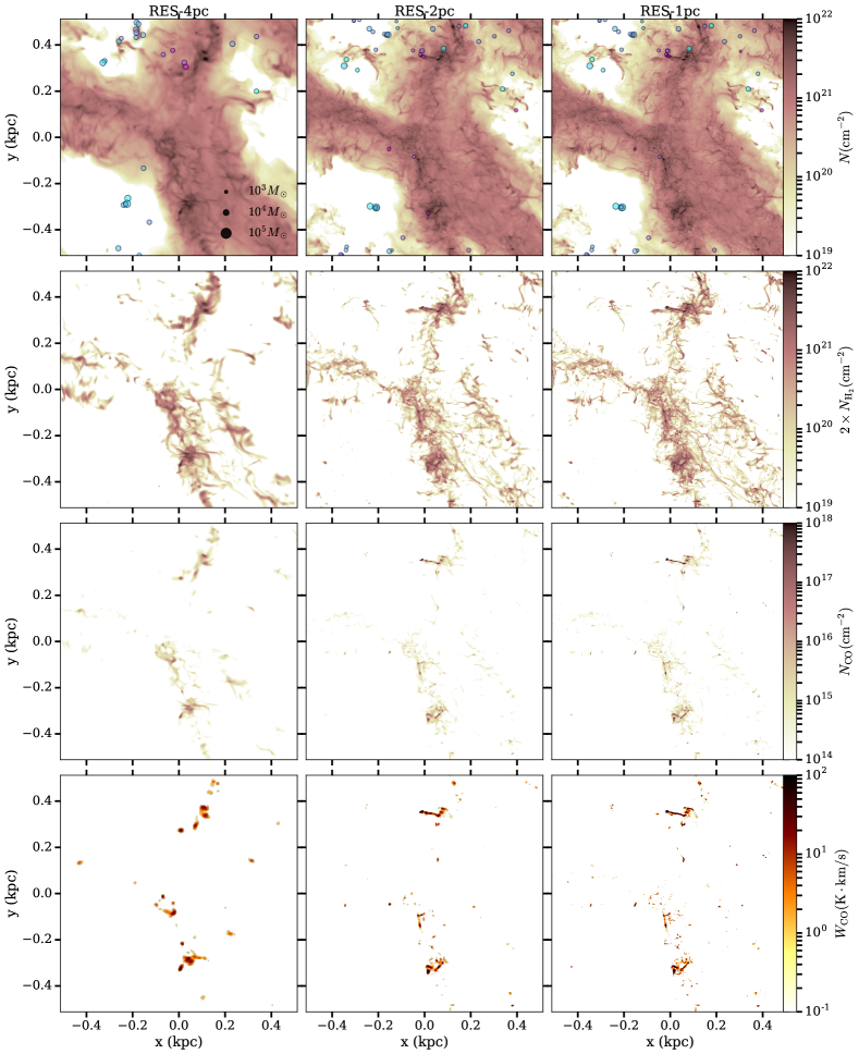
Figure 1.— The column density of all gas ($N$, first row), molecular gas ($N_{\mathrm{H_{2}}}$, second row), $\mathrm{CO}$ ($N_{\mathrm{CO}}$, third row), and the intensity of the $\mathrm{CO}(J=1-0)$ line ($W_{\mathrm{CO}}$, last row) in models RES-4pc, (left), RES-2pc (middle) and RES-1pc (right). The young (age $<40~{}\mathrm{Myr}$) star clusters/sink particles formed in the simulations are shown as filled circles in the first row with $N$. The area of the circles are proportional to the square root of the cluster masses, ranging from $10^{3}~{}M_{\odot}$ to $10^{5}~{}M_{\odot}$ (see legends in the top left panel), and the color of the circles indicates the cluster age, from $0$ (magenta) to $40~{}\mathrm{Myr}$ (blue).

Table 4Overall properties of models for comparisons in numerical resolution and non-equilibrium chemistry

model ID	$M_{\mathrm{tot}}(M_{\odot})$	$M_{\mathrm{H_{2}}}(M_{\odot})$	$M_{\mathrm{CO}}(M_{\odot})$	$L_{\mathrm{CO}}~{}(\mathrm{K~{}km~{}s^{-1}pc^{2}})$	$\langle X_{\mathrm{CO}}\rangle_{20}$	$f_{\mathrm{dark}}$	$f_{100}$	$2\langle f_{\mathrm{H_{2}}}\rangle$
RES-4pc	$7.48\times 10^{6}$	$5.76\times 10^{5}$	$4.82\times 10^{1}$	$7.63\times 10^{4}$	1.45	69%	0.4%	11%
RES-2pc	$7.41\times 10^{6}$	$5.55\times 10^{5}$	$5.49\times 10^{1}$	$8.27\times 10^{4}$	1.07	75%	0.9%	10%
RES-1pc (TCHEM-50Myr)	$7.41\times 10^{6}$	$6.89\times 10^{5}$	$1.21\times 10^{2}$	$1.22\times 10^{5}$	1.02	71%	2.3%	13%
TCHEM-5Myr	$7.41\times 10^{6}$	$2.46\times 10^{5}$	$8.96\times 10^{1}$	$9.06\times 10^{4}$	0.56	67%	2.3%	5%

3.1.1 Molecular Abundances and Dependence of Chemistry on numerical resolution

As the numerical resolution increases from $4~{}\mathrm{pc}$ to $1~{}\mathrm{pc}$, a larger fraction of mass in the simulations is in the dense gas. This is quantified by the increase of $f_{100}$ (the fraction of gas with density $n>100~{}\mathrm{cm^{-3}}$) with resolution in Table 4, and the density distributions in Figure 2. The density distributions are similar at low densities where the gas is well resolved. At high densities, the distribution cuts off near the density threshold for sink particle creation, where the unresolved dense gas is converted into sink particles in the simulations. As resolution increases, the density threshold for sink particle creation also increases, allowing denser gas to form.

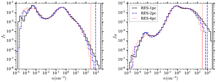
Figure 2.— Histograms of volume-weighted (left) and mass-weighted (right) density $n$ in models RES-1pc (solid black), RES-2pc (dashed blue) and RES-4pc (dotted red). The $y$-axes are normalized to show the fraction of volume $f_{V}$ or mass $f_{M}$ in each density bin. The vertical lines indicate the density threshold for sink particle creation at the corresponding resolution in each model (Section 2.1).

The change of density distribution with resolution affects the chemical compositions of the gas. As the resolution increases from $4~{}\mathrm{pc}$ to $1~{}\mathrm{pc}$, the total $\mathrm{H_{2}}$ mass stays nearly constant, but the total $\mathrm{CO}$ mass increases by a factor of nearly 3 (Table 4). The reason for this is evident in Figure 3: most $\mathrm{H_{2}}$ forms in the density range of $n=10-100~{}\mathrm{cm^{-3}}$, which is already well resolved with $4~{}\mathrm{pc}$ resolution. However, most $\mathrm{CO}$ forms at $n\gtrsim 200~{}\mathrm{cm^{-3}}$, which is not well resolved with $2~{}\mathrm{pc}$, maybe even $1~{}\mathrm{pc}$ resolution. Using adaptive mesh refinement (AMR) models, Seifried et al. (2017) found a resolution of $\sim 0.2~{}\mathrm{pc}$ is needed for the $\mathrm{CO}$ abundance to converge.

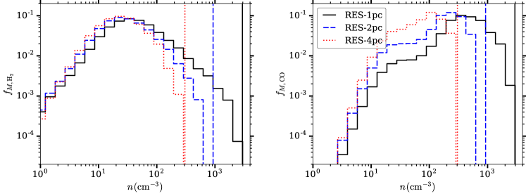
Figure 3.— Histograms of density, similar to Figure 2, but weighted by $\mathrm{H_{2}}$ mass (left) and $\mathrm{CO}$ mass (right) in each cell.

The chemical composition depends not only on density, which affects the rate of collisional reactions, but also on shielding, which determines the photodissociation rate by FUV photons. Which factor, density or shielding, is more important in determining the $\mathrm{H_{2}}$ and $\mathrm{CO}$ abundances in realistic molecular clouds with complex structures? Figures 4 and 5 plot the probability density distributions (PDFs) of the $\mathrm{H_{2}}$ and $\mathrm{CO}$ abundances versus density and shielding in each grid cell. We weight the PDFs by $nf_{\mathrm{H_{2}}}$ or $nf_{\mathrm{CO}}$, so that the color scale is proportional to the $\mathrm{H_{2}}$ or $\mathrm{CO}$ mass in each bin. Simple volume weighted PDFs will show distibutions centered at very low density and low molecular abundances, since by volume most gas is atomic.

We quantify the shielding by calculating the effective extinction $A_{V,\mathrm{eff}}$ for the photo-electric heating (Gong et al. 2017),

$$\chi_{\mathrm{PE}}\equiv\chi\exp(-1.8A_{V,\mathrm{eff}}),$$ (11)

where $\chi_{\mathrm{PE}}$ is the actual radiation field intensity obtained from the six-ray radiation transfer.

As shown in Figure 4, the $\mathrm{H_{2}}$ abundance has a much tighter correlation with density than with shielding. This is because $\mathrm{H_{2}}$ self-shielding is so efficient that the photodissociation rate of $\mathrm{H_{2}}$ is very small in most regions that have a significant amount of $\mathrm{H_{2}}$. In the absence of photodissociation by FUV radiation, the $\mathrm{H_{2}}$ abundance is then determined by the balance between $\mathrm{H_{2}}$ formation on dust grains,

$$\mathrm{H+H+gr\rightarrow H_{2}+gr},$$ (12)

with a rate coefficient $k_{\mathrm{gr}}=3.0\times 10^{-17}~{}\mathrm{cm^{3}s^{-1}}$ (assuming solar neighborhood dust abundance), $\mathrm{H_{2}}$ formation by $\mathrm{H_{3}^{+}}$,

$$\mathrm{H_{3}^{+}+e\rightarrow H_{2}+H},$$ (13)

with a rate coefficient $k_{\ref{eq:H2_H3+}}$, $\mathrm{H_{2}}$ destruction by cosmic-rays,

$$\mathrm{CR+H_{2}\rightarrow H_{2}^{+}+e},$$ (14)

with a rate coefficient $k_{\mathrm{CR}}=2\xi_{\mathrm{H}}(2.3f_{\mathrm{H_{2}}}+1.5f_{\mathrm{H}})$, and $\mathrm{H_{2}}$ destruction by $\mathrm{H_{2}^{+}}$,

$$\mathrm{H_{2}^{+}+H_{2}\rightarrow H_{3}^{+}+H},$$ (15)

with a rate coefficient $k_{\ref{eq:H2_H2p}}$. Reactions (14) and (15) are also the main pathways for $\mathrm{H_{2}^{+}}$ destruction and creation. Equilibrium of $\mathrm{H_{2}^{+}}$ requires

$$f_{\mathrm{H_{2}}}k_{\mathrm{CR}}=f_{\mathrm{H_{2}^{+}}}f_{\mathrm{H_{2}}}nk_{\ref{eq:H2_H2p}}.$$ (16)

$\mathrm{H_{3}^{+}}$ is mainly created by reaction (15), and destroyed by reaction $\mathrm{H_{3}^{+}+e}$, which forms $\mathrm{H_{2}+H}$ (reaction (13)) or $\mathrm{3H}$ with a branching ratio of 0.35:0.65. Equilibrium of $\mathrm{H_{3}^{+}}$ requires

$$f_{\mathrm{H_{2}^{+}}}f_{\mathrm{H_{2}}}nk_{\ref{eq:H2_H2p}}=\frac{1}{0.35}f_{\mathrm{H_{3}^{+}}}f_{\mathrm{e}}nk_{\ref{eq:H2_H3+}}.$$ (17)

Finally, equilibrium of fully-shielded $\mathrm{H_{2}}$ (Equations (12) - (17)) requires

$$f_{\mathrm{H}}nk_{\mathrm{gr}}+f_{\mathrm{H_{3}^{+}}}f_{\mathrm{e}}nk_{\ref{eq:H2_H3+}} =f_{\mathrm{H_{2}}}k_{\mathrm{CR}}+f_{\mathrm{H_{2}^{+}}}f_{\mathrm{H_{2}}}nk_{\ref{eq:H2_H2p}}$$ (18)

$$f_{\mathrm{H}}nk_{\mathrm{gr}}+0.35f_{\mathrm{H_{2}^{+}}}f_{\mathrm{H_{2}}}nk_{\ref{eq:H2_H2p}} =f_{\mathrm{H_{2}}}k_{\mathrm{CR}}+f_{\mathrm{H_{2}^{+}}}f_{\mathrm{H_{2}}}nk_{\ref{eq:H2_H2p}}$$

$$f_{\mathrm{H}}nk_{\mathrm{gr}} =1.65f_{\mathrm{H_{2}}}k_{\mathrm{CR}}.$$

In the above, each $f$ is the abundance of a given species relative to hydrogen nuclei.

Equation (18) can be solved with the conservation of hydrogen nuclei $f_{\mathrm{H}}+2f_{\mathrm{H_{2}}}=1$, giving the equilibrium $\mathrm{H_{2}}$ abundance as a function of $n$, plotted as the green dashed line in the left panel of Figure 4. This agrees very well with the upper limit of $f_{\mathrm{H_{2}}}$ in the simulations. The spread of $f_{\mathrm{H_{2}}}$ at a given density is due to the incomplete shielding of FUV radiation in some regions where destruction of $\mathrm{H_{2}}$ from photodissociation brings its abundance lower than that in completely shielded regions. This can also be seen in the right panel of Figure 4: there is a large spread of $A_{V,\mathrm{eff}}$ at a given $f_{\mathrm{H_{2}}}$, and there are many grid cells with $A_{V,\mathrm{eff}}<1$ and significant $\mathrm{H_{2}}$ abundance.

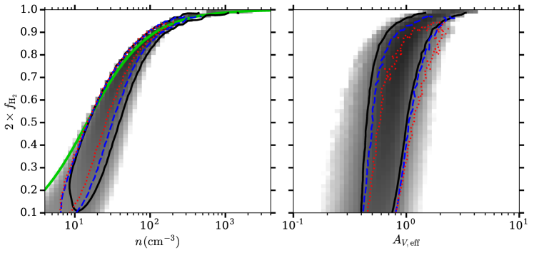
Figure 4.— Distributions of the $\mathrm{H_{2}}$ abundance $f_{\mathrm{H_{2}}}$ versus the gas density $n$ (left) and the effective extinction $A_{V,\mathrm{eff}}$ (right). The color scale shows the log of the $\mathrm{H_{2}}$ mass in each bin for model RES-1pc, spanning three orders of magnitude. The contours indicate 90% of the $\mathrm{H_{2}}$ mass in models RES-1pc (black solid), RES-2pc (blue dashed), and RES-4pc (red dotted). The green line shows the equilibrium $\mathrm{H_{2}}$ abundance assuming the FUV radiation is completely shielded (Equation (18)).

Contrary to the case of $\mathrm{H_{2}}$ abundance, which is determined mostly by density, the CO abundance is determined by both density and shielding, as shown in Figure 5. $\mathrm{CO}$ forms mainly in regions with $n\gtrsim 100~{}\mathrm{cm^{-3}}$ and $A_{V}\gtrsim 1$. This agrees very well with the results from 1D slab models in Gong et al. (2017, see their Figures 5 and 6). The main reason $\mathrm{H_{2}}$ and $\mathrm{CO}$ form under different conditions is that the self-shielding of $\mathrm{CO}$ and cross-shielding of $\mathrm{CO}$ by $\mathrm{H_{2}}$ are much less efficient than the $\mathrm{H_{2}}$ self-shielding. As a result, $\mathrm{CO}$ formation is limited by photodissociation, and $\mathrm{CO}$ can only form in regions with $A_{V,\mathrm{eff}}\gtrsim 1$ where the FUV radiation field is sufficiently shielded by dust. Moreover, $\mathrm{CO}$ formation also requires higher densities, as $\mathrm{C^{+}}$ and $\mathrm{He^{+}}$ formed by cosmic rays destroy $\mathrm{CO}$ at lower densities. Figures 4 and 5 again show that the $\mathrm{H_{2}}$ mass in our simulations is converged, but the $\mathrm{CO}$ mass is not, due to the lack of resolution for very high density gas (see also Figure 3 and discussion).

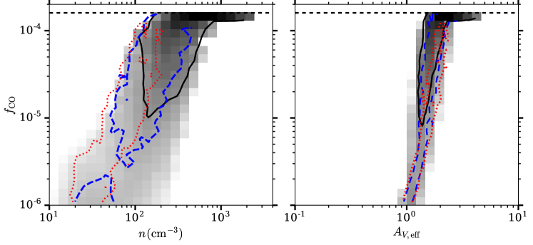
Figure 5.— Similar to Figure 4, but for the $\mathrm{CO}$ abundance $f_{\mathrm{CO}}$. The black dashed lines show where all carbon is in $\mathrm{CO}$, i.e., $f_{\mathrm{CO}}=1.6\times 10^{-4}$.

Because $\mathrm{H_{2}}$ and $\mathrm{CO}$ formation require different conditions, $\mathrm{CO}$ is only a very approximate tracer of $\mathrm{H_{2}}$. Figure 6 shows the distribution of density $n$ versus the effective extinction $A_{V,\mathrm{eff}}$ for each grid cell. At a given density, there is a large range of $A_{V,\mathrm{eff}}$. We roughly delineate loci where $\mathrm{H}$, $\mathrm{H_{2}}$, and $\mathrm{CO}$ form: $\mathrm{H_{2}}$ exists in high density regions, and $f_{\mathrm{H_{2}}}>0.5$ corresponds roughly to densities $n\gtrsim 30~{}\mathrm{cm^{-3}}$. $\mathrm{CO}$ forms in denser and well shielded regions, and $f_{\mathrm{CO}}>10^{-5}$ roughly corresponds to $n\gtrsim 100~{}\mathrm{cm^{-3}}$ and $A_{V,\mathrm{eff}}\gtrsim 1$. Figure 6 clearly shows that a significant fraction of $\mathrm{H_{2}}$ would not be traced by $\mathrm{CO}$ emission (see $f_{\mathrm{dark}}$ in Table 4). As $\Delta x$ decreases from $4~{}\mathrm{pc}$ to $1~{}\mathrm{pc}$, more and more high density gas is resolved, as also shown in Figure 2. Nevertheless, for all resolutions considered in our models, there is gas in the three different regimes – atomic, $\mathrm{CO}$-bright molecular, and $\mathrm{CO}$-dark molecular.

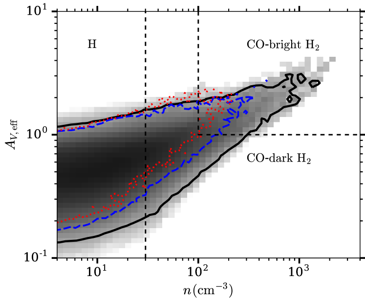
Figure 6.— Distribution of density $n$ versus effective extinction $A_{V,\mathrm{eff}}$. The color scale shows the log of the mass in each bin in model RES-1pc, spanning across three orders of magnitude. The contours indicate 99% of the mass in models RES-1pc (black solid), RES-2pc (blue dashed), and RES-4pc (red dotted). The dashed lines roughly denote the regions where $\mathrm{H}$, $\mathrm{H_{2}}$, and $\mathrm{CO}$ form (see text in Section 3.1.1).

To validate that we can accurately simulate chemistry in molecular clouds, we compare the $\mathrm{CO}$ column densities $N_{\mathrm{CO}}$ in our simulations to that in the UV absorption observations of diffuse molecular clouds. Figure 7 shows the comparison between the simulations and observations, as well as the result from the one-sided slab model in Gong et al. (2017). The x-axis of Figure 7 is the extinction from only $\mathrm{H_{2}}$:

$$A_{V}(N_{\mathrm{H_{2}}})=\frac{2N_{\mathrm{H_{2}}}}{1.87\times 10^{21}~{}\mathrm{cm^{-2}}}.$$ (19)

To avoid foreground/background contamination, we compare $N_{\mathrm{CO}}$ to $N_{\mathrm{H_{2}}}$ instead of the total column $N$. Compared to the simulations, the one-sided slab model gives higher $\mathrm{CO}$ abundance at $A_{V}(N_{\mathrm{H_{2}}})\sim 1$. This is because the six-ray radiation transfer in the 3D simulations considers extinction of FUV radiation from all directions along the Cartesian axes, which is generally lower than the extinction only along the z-axis, $A_{V}(N_{\mathrm{H_{2}}})$ (that is, $A_{\mathrm{V,eff}}\lesssim A_{V}(N_{\mathrm{H_{2}}})$). At $A_{V}(N_{\mathrm{H_{2}}})\ll 1$ or $A_{V}(N_{\mathrm{H_{2}}})\gg 1$, the $\mathrm{CO}$ abundance in the one-sided slab model and 3D simulations are more similar, because either the FUV radiation is only weakly shielded at low $A_{V}(N_{\mathrm{H_{2}}})$ so that the photodissociation rate is insensitive to $A_{V}(N_{\mathrm{H_{2}}})$, or else already completely shielded at high $A_{V}(N_{\mathrm{H_{2}}})$ so that the limiting factor for $\mathrm{CO}$ formation is no longer photodissociation. The UV absorption observations can only be conducted in diffuse molecular clouds with $A_{V}(N_{\mathrm{H_{2}}})\lesssim 1$, and there is a lack of observations at higher extinctions. For the range of $A_{V}(N_{\mathrm{H_{2}}})$ where the observational data are available, the RES-1pc simulation successfully reproduce the observed range of $N_{\mathrm{CO}}$. Lower resolution simulations RES-2pc and RES-4pc also show similar average values (magenta lines) and range (not shown in the Figure) of $N_{\mathrm{CO}}$ at $A_{V}\lesssim 1$. At $A_{V}>1$, models with lower resolutions start to show that the $\mathrm{CO}$ mass is not resolved at high densities.

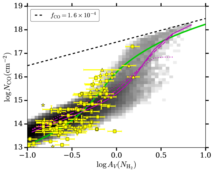
Figure 7.— Distribution of $\mathrm{CO}$ column density $N_{\mathrm{CO}}$ versus $A_{V}(N_{\mathrm{H_{2}}})$ in the model RES-1pc. The color scale shows the log of the gas column in each bin, spanning across three orders of magnitude. The magenta lines indicate the median of the $\log N_{\mathrm{CO}}$ in $\log A_{V}(N_{\mathrm{H_{2}}})$ bins for models RES-1pc (solid), RES-2pc (dashed) and RES-4pc (dotted). The black dashed line shows where all carbon is in $\mathrm{CO}$, i.e., $f_{\mathrm{CO}}=1.6\times 10^{-4}$. The yellow symbols are UV absorption observations in Rachford et al. (2002) (triangles), Sheffer et al. (2008) (squares), Crenny & Federman (2004) (stars) and Burgh et al. (2010) (pentagons), compiled by Gong et al. (2017). The green line shows the result from the one-sided slab model with constant density $n=100~{}\mathrm{cm^{-3}}$ in Gong et al. (2017).

3.1.2 Dependence of $X_{\mathrm{CO}}$ on Numerical Resolution

To understand the relation between physical properties of molecular clouds and $\mathrm{CO}$ emission, a helpful reference point is the simple uniform slab model for molecular clouds. In a uniform slab with constant $\mathrm{CO}$ excitation temperature $T_{\mathrm{exc}}$, Equation (8) can be integrated, giving

$$I_{\nu}=I_{\nu}(0)\mathrm{e}^{-\tau_{\nu}}+B_{\nu}(T_{\mathrm{exc}})(1-\mathrm{e}^{-\tau_{\nu}}),$$ (20)

where $S_{\nu}=B_{\nu}(T_{\mathrm{exc}})$, the blackbody radiation field intensity at temperature $T_{\mathrm{exc}}$, and $I_{\nu}(0)$ is the initial impinging radiation field intensity at $\tau_{\nu}=0$. The line intensity $I_{\nu}$ is usually measured in terms of the antenna temperature (also often referred to as the radiation temperature) in radio astronomy:

$$T_{A}(\nu)=\frac{c^{2}}{2k\nu^{2}}I_{\nu}.$$ (21)

In the limit of $\tau_{\nu}\rightarrow\infty$, Equations (20) and (21) becomes

$$T_{A}=\frac{T_{0}}{\mathrm{e}^{T_{0}/T_{\mathrm{exc}}}-1},$$ (22)

where $T_{0}=5.5~{}\mathrm{K}=h\nu_{0}/k$, with $\nu_{0}=115.3~{}\mathrm{Hz}$, the frequency of the $\mathrm{CO}(J=1-0)$ line.

Typically, the $\mathrm{CO}(J=1-0)$ line profile (in terms of $T_{A}$ and $v$) is not too far from a Gaussian profile, and to first order, the total $\mathrm{CO}$ line intensity $W_{\mathrm{CO}}$ is determined by two parameters: the peak of the line profile $T_{\mathrm{peak}}$ and the width/velocity dispersion of the line $\sigma_{v}$. Under the assumption that the line center is optically thick so that Equation (22) applies, the observed peak antenna temperature, $T_{\mathrm{peak}}$, would be directly related to the excitation temperature $T_{\mathrm{line}}$,

$$T_{\mathrm{line}}\equiv\frac{5.5~{}\mathrm{K}}{\ln(5.5~{}\mathrm{K}/T_{\mathrm{peak}}+1)}.$$ (23)

We use the notation $T_{\mathrm{line}}$ for the excitation temperature derived from the line profile ($T_{\mathrm{peak}}$) to distinguish from the true excitation temperature in the molecular clouds $T_{\mathrm{exc}}$. Although $T_{\mathrm{line}}=T_{\mathrm{exc}}$ in a uniform slab cloud as long as the $\mathrm{CO}$ line center is optically thick, in real molecular clouds and also in our numerical simulations, the excitation temperature along the line of sight is not constant, and $T_{\mathrm{line}}$ serves as an estimate of the excitation temperature where most $\mathrm{CO}$ emission comes from. For $T_{\mathrm{peak}}\gtrsim 5.5~{}\mathrm{K}$, Equation (23) gives $T_{\mathrm{line}}\approx T_{\mathrm{peak}}$. Another important parameter for the $\mathrm{CO}$ line, the velocity dispersion, is calculated using $\sigma_{v}\equiv\sqrt{\langle v^{2}\rangle_{T_{A}}-\langle v\rangle_{T_{A}}^{2}}$, where $\langle v\rangle_{T_{A}}\equiv\int vT_{A}\mathrm{d}v/\int T_{A}\mathrm{d}v$ is the intensity weighted average of velocity, and similarly $\langle v^{2}\rangle_{T_{A}}\equiv\int v^{2}T_{A}\mathrm{d}v/\int T_{A}\mathrm{d}v$.

The relations between $W_{\mathrm{CO}}$ and $T_{\mathrm{line}}$ or $\sigma_{v}$ in models RES-1pc, RES-2pc and RES-4pc are shown in Figure 8. $T_{\mathrm{line}}$ ranges from $\sim 2~{}\mathrm{K}$ (from the CMB background) to $\sim 20~{}\mathrm{K}$ (from the kinetic temperature of dense gas as discussed below), similar to the range of excitation temperature observed in Perseus and Taurus molecular clouds (Pineda et al. 2008, 2010). The velocity dispersion spans a relatively narrow range $\sigma_{v}\approx 1-2~{}\mathrm{km/s}$, and the lower limit for $\sigma_{v}$ is set by the sub-grid micro-turbulence velocity in Equation (9). The observations of nearby molecular clouds have higher resolutions of $\sim 0.2-0.4~{}\mathrm{pc}$, and therefore a slightly lower but still limited range of velocity dispersions $\sigma_{v}\approx 0.8-1.5~{}\mathrm{km/s}$ (Pineda et al. 2010; Kong et al. 2015). $W_{\mathrm{CO}}$ increases with both $T_{\mathrm{line}}$ and $\sigma_{v}$. For a Gaussian profile with $T_{\mathrm{peak}}\gtrsim 5.5~{}\mathrm{K}$, $W_{\mathrm{CO}}=\sqrt{2\pi}T_{\mathrm{peak}}\sigma_{v}\approx\sqrt{2\pi}T_{\mathrm{line}}\sigma_{v}$. Because the variation in $\sigma_{v}$ is small, $W_{\mathrm{CO}}$ correlates very well with $T_{\mathrm{line}}$, except for regions where $T_{\mathrm{line}}$ saturates around $20~{}\mathrm{K}$. There is no saturation of $W_{\mathrm{CO}}$, and $W_{\mathrm{CO}}$ keeps increasing with increasing $\sigma_{v}$.

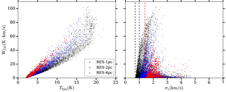
Figure 8.— Left: scatter plot of $W_{\mathrm{CO}}$ vs. $T_{\mathrm{line}}$, the excitation temperature of the $\mathrm{CO}(J=1-0)$ at line center (see Equation (23)); and right: $W_{\mathrm{CO}}$ vs. the velocity dispersion of the line, $\sigma_{v}$. Both panels show models RES-1pc (black), RES-2pc (blue) and RES-4pc (red), with the area of points proportional to the area of the pixel at the corresponding resolution. The vertical dashed lines show the sub-grid micro-turbulence parameter (see Equation (9)).

$W_{\mathrm{CO}}$ is largely determined by the excitation temperature, and the excitation temperature in turn depends on the gas density and temperature. Figure 9 shows the excitation temperature $T_{\mathrm{exc}}$ and gas temperature $T_{\mathrm{gas}}$ versus the gas density in each grid cell. $T_{\mathrm{gas}}$ decreases with increasing density, as the gas cooling becomes more efficient, and heating is also reduced by shielding of the FUV radiation field in dense regions. On the other hand, $T_{\mathrm{exc}}$ increases with increasing density, because the collisional excitation rate of $\mathrm{CO}$ is proportional to density, and because radiative trapping increases in dense regions.

The lower solid magenta line in Figure 9 shows the median $T_{\mathrm{exc}}$ from model RES-1pc as a function of density. $T_{\mathrm{exc}}$ only reaches equilibrium with $T_{\mathrm{gas}}$ at $n\gtrsim 400~{}\mathrm{cm^{-3}}$, implying that local thermal equilibrium (LTE) approximation would fail in most regions.

At a given density, $T_{\mathrm{exc}}$ is higher at lower resolutions for two reasons. First, the velocity gradient $|\mathrm{d}v/\mathrm{d}r|$ is smaller at lower resolutions, leading to higher $\tau_{\mathrm{LVG}}$ and thus lower escape probability $\beta$ and higher $T_{\mathrm{exc}}$ at a given density (See Equations (28) and (30) below). Second, at lower resolutions, less high-density gas is resolved, and a larger fraction of the $\mathrm{CO}$ gas is found in lower-density gas (see Fig. 3b). This shifts the distributions of $T_{\mathrm{exc}}$ and $T_{\mathrm{gas}}$ in Figure 9 to the left at lower resolution in models RES-2pc and RES-4pc (dashed and dotted magenta lines).

In general, thermalization is expected for densities above a critical value at which collisional deexcitation exceeds spontaneous emission. For $\mathrm{CO}$ collisions with $\mathrm{H_{2}}$, the collisional deexcitation rate is $n_{\mathrm{H_{2}}}k_{10}$ for

$$k_{10}\approx 6\times 10^{-11}\left(\frac{T_{\mathrm{gas}}}{100~{}\mathrm{K}}\right)^{0.2}~{}\mathrm{cm^{3}s^{-1}},$$ (24)

at $10~{}\mathrm{K}\lesssim T_{\mathrm{gas}}\lesssim 250~{}\mathrm{K}$ (Flower & Launay 1985; Flower 2001; Draine 2011). The spontaneous emission rate is $\beta A_{10}$, where Equation (6) gives the escape probability $\beta$, so that

$$n_{\mathrm{crit}}=\frac{\beta A_{10}}{k_{10}}.$$ (25)

For $T_{\mathrm{gas}}=20~{}\mathrm{K}$, Equation (24) gives $A_{10}/k_{10}\approx 2.1\times 10^{3}~{}\mathrm{cm^{-3}}$.

With increasing density, the optical depth $\tau_{\mathrm{LVG}}$ increases, leading to decreasing $\beta$ (Figure 10); at large $\tau_{\mathrm{LVG}}$, $\beta\approx 1/\tau_{\mathrm{LVG}}$. For model RES-1pc, we fit the average $\tau_{\mathrm{LVG}}$ at a given density with a broken power-law (magenta line in Figure 10):

$$\tau_{\mathrm{LVG}} =2.4\times 10^{-5}(n/\mathrm{cm^{-3}})^{2.3},\quad n<350~{}\mathrm{cm^{-3}}$$ (26)

$$\tau_{\mathrm{LVG}} =0.21(n/\mathrm{cm^{-3}})^{0.73},\quad n\geq 350~{}\mathrm{cm^{-3}}.$$

Combining Equations (25) and (26) yields $n_{\mathrm{crit}}\sim 300~{}\mathrm{cm^{-3}}$. Thus, in regions where $n\gtrsim 400~{}\mathrm{cm^{-3}}$, the $\mathrm{CO}(J=1)$ level is expected to be thermalized, and this is indeed consistent with the median $T_{\mathrm{exc}}$ for model RES-1pc.

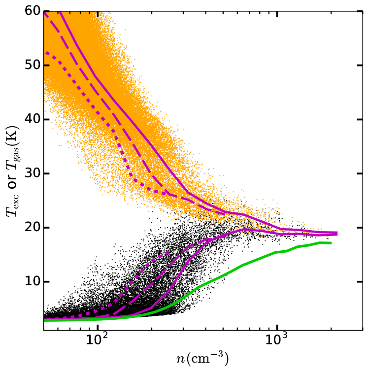
Figure 9.— Scatter plot of the gas temperature (orange, upper branch) and excitation temperature of $\mathrm{CO}(J=1-0)$ line (black, lower branch) versus gas density $n$ in each cell for model RES-1pc. The magenta lines indicate the median gas temperature and $\mathrm{CO}$ excitation temperature in density bins for moedels RES-1pc (solid), RES-2pc (dashed), and RES-4pc (dotted). The green line is the estimation of $T_{\mathrm{exc}}$ in a two-level system model (see Section 3.1.2).

The dependence of $T_{\mathrm{exc}}$ on $n$ can be understood in a simplified 2-level system model. The excitation temperature is defined as

$$T_{\mathrm{exc}}\equiv\frac{T_{0}}{\ln\left(\frac{n_{0}/g_{0}}{n_{1}/g_{1}}\right)}.$$ (27)

With the escape probability approximation, the level populations are given by (Draine 2011)

$$\frac{n_{1}}{n_{0}}=\frac{n_{c}k_{01}+\frac{g_{1}}{g_{0}}\beta A_{10}n_{\gamma}^{(0)}}{n_{c}k_{10}+\beta A_{10}(1+n_{\gamma}^{(0)})},$$ (28)

where

$$k_{01}=\frac{g_{1}}{g_{0}}k_{10}\mathrm{e}^{-T_{0}/T_{\mathrm{gas}}},$$ (29)

$n_{c}$ is the number density for the collisional species, and $n_{\gamma}^{(0)}=1/(\mathrm{e}^{T_{0}/T_{\mathrm{CMB}}}-1)$ the background incident radiation field from the CMB. If the CMB terms are negligible, Equation (27) becomes

$$T_{\mathrm{exc}}=\frac{T_{\mathrm{gas}}}{1+\frac{T_{\mathrm{gas}}}{T_{0}}\ln(1+\frac{\beta A_{10}}{n_{c}k_{10}})}.$$ (30)

For $\beta/n_{c}$ small, $T_{\mathrm{exc}}\rightarrow T_{\mathrm{gas}}$.

The excitation temperature can be estimated as a function of density by Equations (6), (27), (28) and (26) (assuming $\tau=\tau_{\mathrm{LVG}}$ in Equation (6) and using the average value of $T_{\mathrm{gas}}$ at a given density). The analytic 2-level system approximation for simulation RES-1pc (green line) agrees well with the result from radiation transfer by the RADMC-3D code (lower solid magenta line) at low and high densities, while there are differences within a factor of two at intermediate densities $n\sim 300$–$1000~{}\mathrm{cm^{-3}}$. This is because the $\mathrm{CO}$ rotational levels $J=1$, $2$, and $3$ have energies of $5.5$, $16.6$, and $33.2~{}\mathrm{K}$, all lower or comparable to the gas temperature. Indeed, there are significant populations in the $J\geq 2$ levels, as expected given that $T_{\mathrm{gas}}>5.5~{}\mathrm{K}$. The analytical expression in Equation (28) only takes into account the $J=0$ and $J=1$ levels, and therefore cannot predict the excitation temperature very accurately. At low and high densities the differences are small because the excitation temperature there is determined by the background CMB temperature or the gas temperature as the $\mathrm{CO}$ rotational levels approach LTE. Nonetheless, the analytical 2-level system approximation agrees with the general trend from the radiation transfer calculations, and gives some insight into the relation between $T_{\mathrm{exc}}$, $T_{\mathrm{gas}}$ and $n$. As a further test, we ran RADMC-3D only including the first $J=0$ and $J=1$ rotational levels of $\mathrm{CO}$, and found that it can indeed reproduce the analytical result of the 2-level system model. Figure 23 shows this comparison.

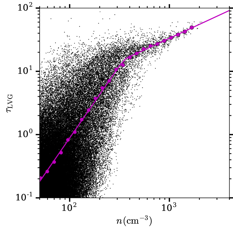
Figure 10.— Scatter plot of the optical depth from the LVG approximation $\tau_{\mathrm{LVG}}$ vs. density $n$ in each grid cell in model RES-1pc. The magenta circles are the binned average of $\tau_{\mathrm{LVG}}$, and the line is a broken power-law fit to the circles (Equation (26)).

The relation between $W_{\mathrm{CO}}$ and $T_{\mathrm{line}}$, as well as the relation between $T_{\mathrm{exc}}$ and density, give rise to the strong correlation between $W_{\mathrm{CO}}$ and the average (mass weighted) density $\langle n\rangle_{M}$ along the line of sight (Figure 11 left panel). Moreover, we found that in the simulations, $N_{\mathrm{H_{2}}}$ increases systematically with $\langle n\rangle_{M}$ (see Figure 6). This results in a correlation between $W_{\mathrm{CO}}$ and $N_{\mathrm{H_{2}}}$ (Figure 11 right panel). Although $X_{\mathrm{CO}}$ is measured in terms of $W_{\mathrm{CO}}$ and $N_{\mathrm{H_{2}}}$, there is a smaller dispersion in the correlation between $W_{\mathrm{CO}}$ and $\langle n\rangle_{M}$. This suggests that the $\mathrm{CO}$ emission is more fundamentally a measure of $\mathrm{H_{2}}$ density than column density.

Figure 11.— Distributions of $W_{\mathrm{CO}}$ versus mass-weighted mean density $\langle n\rangle_{M}$ (left) and $A_{V}(N_{\mathrm{H_{2}}})$ (right). The color scale in the PDF is proportional to the total $\mathrm{CO}$ luminosity $L_{\mathrm{CO}}$ from each bin in model RES-1pc. The black solid contour of the color scale indicates the regions where 50% of the total $\mathrm{CO}$ emission comes from in model RES-1pc. The blue dashed and red dotted contours indicate 50% of the emission, but for models RES-2pc and RES-4pc. The 1D histograms show $L_{\mathrm{CO}}$ in each bin for models RES-1pc (black solid), RES-2pc (blue dashed) and RES-4pc (red dotted).

The effect of numerical resolution on $W_{\mathrm{CO}}$ is already evident in Figures 9 and 11. As the resolution increases, more high density gas forms in the simulation, and thus there are more pixels with high $W_{\mathrm{CO}}$. Numerical resolution also has an effect on $X_{\mathrm{CO}}$, as shown in Figure 12, the histogram of $X_{\mathrm{CO,20}}=X_{\mathrm{CO}}/(10^{20}~{}\mathrm{cm^{-2}K^{-1}km^{-1}s})$ weighted by $W_{\mathrm{CO}}$. The average $X_{\mathrm{CO}}$ in a certain region can be written as:

$$\langle X_{\mathrm{CO}}\rangle=\frac{\sum N_{\mathrm{H_{2}}}}{\sum W_{\mathrm{CO}}}=\frac{\sum\frac{N_{\mathrm{H_{2}}}}{W_{\mathrm{CO}}}W_{\mathrm{CO}}}{\sum W_{\mathrm{CO}}}=\frac{\sum X_{\mathrm{CO}}W_{\mathrm{CO}}}{\sum W_{\mathrm{CO}}}.$$ (31)

In other words, $\langle X_{\mathrm{CO}}\rangle$ is simply the $W_{\mathrm{CO}}$ weighted average of $X_{\mathrm{CO}}$ in each pixel. Therefore, the peak of the histogram in Figure 12 roughly indicates the average $X_{\mathrm{CO}}$ in the whole simulation domain. The distributions of $X_{\mathrm{CO}}$ in models RES-1pc and RES-2pc are very similar, with a slightly higher peak in RES-1pc. As a result, $\langle X_{\mathrm{CO}}\rangle$ is almost the same in RES-1pc and RES-2pc (Table 4). The model RES-4pc, however, peaks at larger $X_{\mathrm{CO}}$ than the higher resolution models, and therefore has a higher $\langle X_{\mathrm{CO}}\rangle$. This is because the peak of $X_{\mathrm{CO}}$ distribution, $X_{\mathrm{CO,20}}\approx 0.5$, comes from regions with moderatly high density $n\approx 100~{}\mathrm{cm^{-3}}$ and $\mathrm{CO}$ emission $W_{\mathrm{CO}}\approx 40~{}\mathrm{K\cdot km/s}$, which can only be resolved at a resolution finer than $2~{}\mathrm{pc}$ (see histograms of $\langle n\rangle_{M}$ and $W_{\mathrm{CO}}$ in Figure 11). Therefore, we conclude that a numerical resolution of at least $2~{}\mathrm{pc}$ is needed in order to resolve the average $X_{\mathrm{CO}}$ in molecular clouds for solar neighborhood conditions.

Figure 12.— Histograms of $X_{\mathrm{CO,20}}$ weighted by $W_{\mathrm{CO}}$, in models RES-1pc (black solid), RES-2pc (blue dashed) and RES-4pc (red dotted).

Finally, we compare the distribution of $W_{\mathrm{CO}}$ versus $A_{V}(N_{\mathrm{H_{2}}})$ in model RES-1pc to observations of the Orion A and B molecular clouds by Ripple et al. (2013), as shown in Figure 13. Considering the noise level in the observation, we use a higher threshold of $W_{\mathrm{CO}}>1~{}\mathrm{K\cdot km/s}$ to compare to the $\mathrm{CO}$-bright region in Orion. Because most $\mathrm{CO}$ emission comes from regions with $W_{\mathrm{CO}}\gg 1~{}\mathrm{K\cdot km/s}$, $X_{\mathrm{CO}}$ is not sensitive to the $W_{\mathrm{CO}}$ threshold. Our simulations shows a similar distribution of $W_{\mathrm{CO}}$ versus $A_{V}(N_{\mathrm{H_{2}}})$ to that in Orion. The dispersion of $W_{\mathrm{CO}}$ at a given $A_{V}(N_{\mathrm{H_{2}}})$ is large, as much as more than an order of magnitude at low $A_{V}(N_{\mathrm{H_{2}}})$. However, despite the large dispersion of $W_{\mathrm{CO}}$, the average $X_{\mathrm{CO}}$ (which is inversely proportional to the slope) in different $A_{V}(N_{\mathrm{H_{2}}})$ bins is very similar, only varying by a factor of $\sim 2$. Similar features are observed in many Milky Way molecular clouds by Lee et al. (2018), and we discuss this in more detail in Section 3.3.

There are also some differences between the simulation and observations. The average $X_{\mathrm{CO}}$ in RES-1pc is a factor of 1.4 lower than that in Orion. As we shall show based on other analyses and comparisons, the typical $X_{\mathrm{CO}}$ in our simulations is about a factor of $\sim 2$ lower than the standard Milky Way value; we discuss possible reasons for this discrepency at the end of Section 3.3. We also note that because the observation in Ripple et al. (2013) has a higher spatial resolution of $\sim 0.2~{}\mathrm{pc}$, there are more pixels at $A_{V}(N_{\mathrm{H_{2}}})\gtrsim 4$ in the observation in Figure 13. The simulation has more pixels at $W_{\mathrm{CO}}\gtrsim 60~{}\mathrm{K\cdot km/s}$, a result of the slightly higher velocity dispersions (see Figure 8 and discussion). In spite of these differences, the general good agreement between the models and observations indicates that the simulations can succesfully reproduce the basic physical properties of observed molecular clouds.

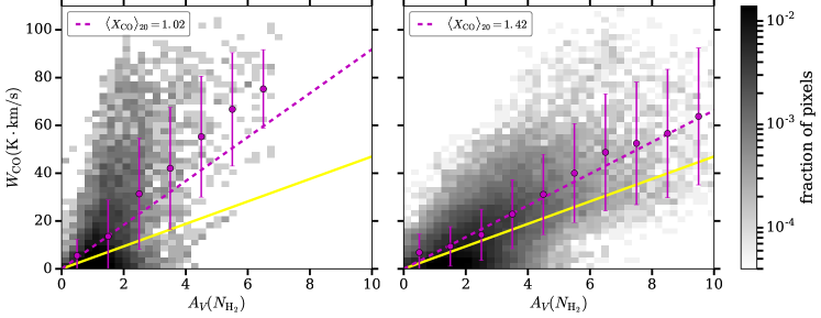
Figure 13.— Left: Distribution of $W_{\mathrm{CO}}$ versus $A_{V}(N_{\mathrm{H_{2}}})$ in model RES-1pc. The magenta filled circles and error bars show the average value and standard deviation of $W_{\mathrm{CO}}$ in each $A_{V}(N_{\mathrm{H_{2}}})$ bin. The yellow solid line shows the standard Milky Way value of $X_{\mathrm{CO,MW,20}}=2$. The magenta dashed line shows the average $X_{\mathrm{CO}}$ in model RES-1pc, $\langle X_{\mathrm{CO}}\rangle_{20}=1.02$. Right: similar to the left panel, but for the observations of Orion A and B molecular clouds by Ripple et al. (2013). The average $X_{\mathrm{CO}}$ for the Orion A and B clouds is $\langle X_{\mathrm{CO}}\rangle_{20}=1.42$.

3.2. Non-equilibrium Chemistry

The realistic ISM is highly dynamical: turbulence constantly creates and disperses molecular clouds, and moves gas to environments with different density, temperature and radiation field strength. As a result, non-equilibrium chemistry is likely to be important, especially in low density diffuse gas where the chemical timescales are long compared to the dynamical timescales. This is especially an issue for $\mathrm{H_{2}}$. Molecular hydrogen can form in low density gas due to its effective self-shielding, but its formation timescale, $t_{\mathrm{H_{2}}}\approx 10\mathrm{Myr}~{}(n/100~{}\mathrm{cm^{-3}})^{-1}$ (Gong et al. 2017), can be longer than the dynamical timescale (Equation (3)). Because $\mathrm{CO}$ formation chemically relies on the existence of $\mathrm{H_{2}}$, the $\mathrm{CO}$ abundance in molecular clouds can also be far from equilibrium. In this section, we carry out comparisons between models with different $t_{\mathrm{chem}}$ (model IDs start with TCHEM in Table 3) to investigate the effect of non-equilibrium chemistry on $X_{\mathrm{CO}}$.

Both $\mathrm{H_{2}}$ and $\mathrm{CO}$ abundance increase over $t_{\mathrm{chem}}$, reaching a steady state at $t_{\mathrm{chem}}\approx 50~{}\mathrm{Myr}$, as shown in Figure 14. Over timescales relevant for clouds of size $\gtrsim 10~{}\mathrm{pc}$ (Equation (3)), there is a larger increase in the $\mathrm{H_{2}}$ abundance than $\mathrm{CO}$: From $t_{\mathrm{chem}}=5~{}\mathrm{Myr}$ to $50~{}\mathrm{Myr}$, the $\mathrm{H_{2}}$ abundance increases by a factor of $\sim 3$, while $\mathrm{CO}$ abundance increases only by $\sim 30\%$.

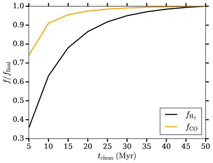
Figure 14.— The abundance of $\mathrm{H_{2}}$ (black) and $\mathrm{CO}$ (orange) as a function of $t_{\mathrm{chem}}$ in TCHEM models. The y-axis is normalized by the final $\mathrm{H_{2}}$ or $\mathrm{CO}$ abundance at $t_{\mathrm{chem}}=50~{}\mathrm{Myr}$.

The difference in the evolution of $\mathrm{H_{2}}$ and $\mathrm{CO}$ abundance comes from their different distributions. As shown in Figure 15, both $\mathrm{H_{2}}$ and $\mathrm{CO}$ abundances are closer to equilibrium at higher densities, as the rate of collisional reactions increases with density. In fact, at a given density in the range $\sim 40-400~{}\mathrm{cm^{-3}}$, at $5~{}\mathrm{Myr}$ the abundance of $\mathrm{H_{2}}$ is closer than the abundance of $\mathrm{CO}$ is to its final value. However, in equilibrium most of the $\mathrm{H_{2}}$ is in gas at intermediate densities $n\approx 10-100~{}\mathrm{cm^{-3}}$, whereas most $\mathrm{CO}$ is in gas at high densities $n\gtrsim 200~{}\mathrm{cm^{-3}}$ (Figure 3). This leads to a shorter timescale for the overall $\mathrm{CO}$ abundance to reach equilibrium than $\mathrm{H_{2}}$. Since the $\mathrm{CO}$ luminosity also increases much less than the $\mathrm{H_{2}}$ mass, this leads to a lower $X_{\mathrm{CO}}$ value at early $t_{\mathrm{chem}}$ (Table 4).

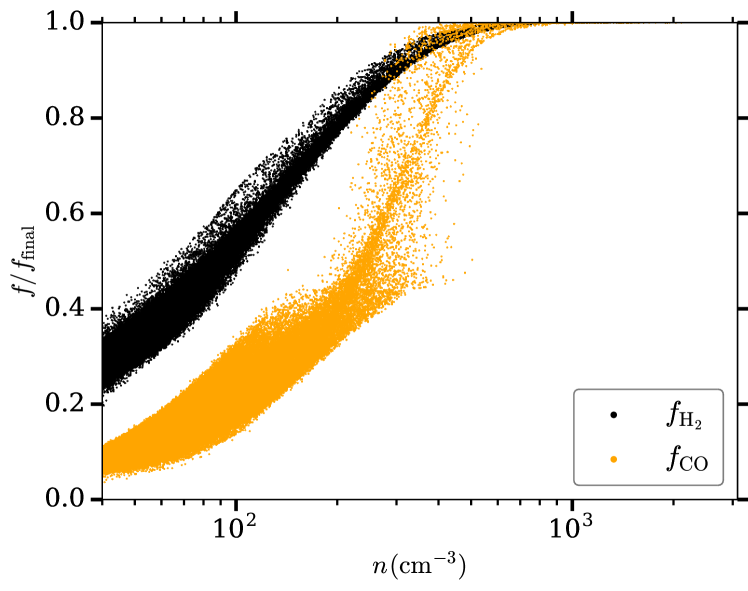
Figure 15.— Scatter plot of $f_{\mathrm{H_{2}}}$ (black) and $f_{\mathrm{CO}}$ (orange) versus density $n$ for model TCHEM-5Myr. $f_{\mathrm{H_{2}}}$ and $f_{\mathrm{CO}}$ in each grid cell is normalized to the equilibrium abundance $f_{\mathrm{H_{2},final}}$ and $f_{\mathrm{CO,final}}$ in that grid cell at $t_{\mathrm{chem}}=50~{}\mathrm{Myr}$ (in model TCHEM-50Myr).

Non-equilibrium chemistry also has an effect on the distribution of $W_{\mathrm{CO}}$ vs. $A_{V}(N_{\mathrm{H_{2}}})$. For model TCHEM-5Myr (Figure 16), the distribution of the pixels are shifted to the left compared to that in TCHEM-50Myr (left panel of Figure 13). This is because $W_{\mathrm{CO}}$ is close to equilibrium, but $N_{\mathrm{H_{2}}}$ is a factor of $\sim 2$ smaller than the equilibrium values, for the same reasons discussed above. Moreover, the distribution of $W_{\mathrm{CO}}$ vs. $A_{V}(N_{\mathrm{H_{2}}})$ in TCHEM-5Myr shows some hints of a plateau for $W_{\mathrm{CO}}$ at high $A_{V}(N_{\mathrm{H_{2}}})$, especially in the binned average value of $W_{\mathrm{CO}}$, which is not present in TCHEM-50Myr. This implies that younger clouds may not only have lower $X_{\mathrm{CO}}$ on average, but also different distributions of $W_{\mathrm{CO}}$ vs. $A_{V}(N_{\mathrm{H_{2}}})$ compared to older clouds. We discuss this further in Section 3.3. Note that $N_{\mathrm{H_{2}}}$ includes all $\mathrm{H_{2}}$ along the line of sight, both in high density clumps where $\mathrm{CO}$ forms, and in the foreground/background low density envelopes with only $\mathrm{H_{2}}$ and no $\mathrm{CO}$. Because most $\mathrm{H_{2}}$ (in equilibrium) lies in these low density envelopes, the fractions of $\mathrm{H_{2}}$ in $\mathrm{CO}$-bright and $\mathrm{CO}$-dark regions increase by similar proportions with $t_{\mathrm{chem}}$, and $f_{\mathrm{dark}}$ stays constant from $t_{\mathrm{chem}}=5~{}\mathrm{Myr}$ to $t_{\mathrm{chem}}=50~{}\mathrm{Myr}$ (Table 4).

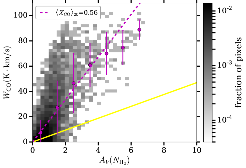
Figure 16.— Similar to the left panel of Figure 13, but for model TCHEM-5Myr.

3.3. Variations in Galactic Environments

Galactic environment fundamentally impacts the molecular content of the ISM. Supernova feedback creates and destroys molecular clouds, shocks and turbulence shape molecular clouds in different morphologies, and the radiation field varies with the star formation activities. Some of these effects can be seen visually in Figure 17. The morphology of molecular clouds varies from dense concentrated structures (such as in T-356Myr), to more diffuse, smaller clouds (such as in T-406Myr). The mass and number of young clusters also changes over time, reflecting the variations in the star formation rate. To quantify the effect of time-varying galactic environment on $X_{\mathrm{CO}}$, we compare models with $2~{}\mathrm{pc}$ resolution at different times during the galactic evolution (model IDs start with T in Table 3). As discussed in Section 3.1.2, the average $X_{\mathrm{CO}}$ is well resolved with a resolution of $2~{}\mathrm{pc}$ in these simulations.

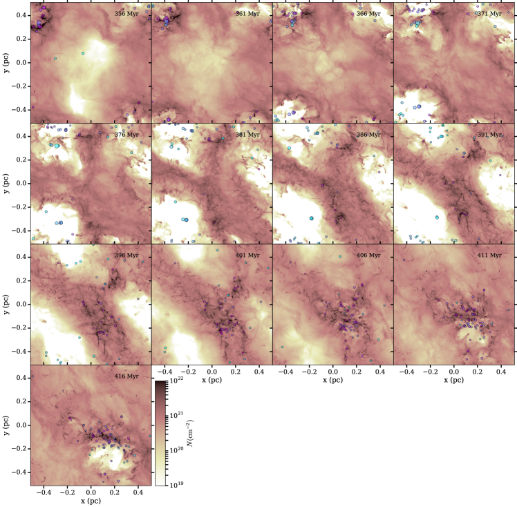
Figure 17.— Total gas surface density $N$ in models T-356Myr – T-416Myr. The star clusters are shown in circles, similar to Figure 1 top panels.

A summary of models T-356Myr – T-416Myr is listed in Table 5. In these models, $M_{\mathrm{H_{2}}}$ and $L_{\mathrm{CO}}$ vary by factor of $\sim 3$, and the incident radiation field strength varies by a factor of $\sim 8$. However, despite these large variations in the environment, $\langle X_{\mathrm{CO}}\rangle$ stays almost constant, changing only by $\sim 40\%$. We found no strong correlation (coefficient of determination $R^{2}<0.4$ in linear regression) between $\langle X_{\mathrm{CO}}\rangle$ and $M_{\mathrm{H_{2}}}$, the radiation field strength $\chi$, or the average extinction from $\mathrm{H_{2}}$ in $\mathrm{CO}$-bright regions $\langle A_{V}\rangle_{\mathrm{CO}}$. Remy et al. (2017) measured $\langle X_{\mathrm{CO}}\rangle$ in individual Milky Way molecular clouds using $\gamma$-ray observations, and they also found no strong correlation between $\langle X_{\mathrm{CO}}\rangle$ and $M_{\mathrm{H_{2}}}$ or $\langle A_{V}\rangle_{\mathrm{CO}}$.

Remy et al. (2017) found a slight anti-correlation of $\langle X_{\mathrm{CO}}\rangle$ and $\langle W_{\mathrm{CO}}\rangle$: $\langle X_{\mathrm{CO}}\rangle\sim-0.051\langle W_{\mathrm{CO}}\rangle$. We similarly found a slight anti-correlation (Figure 18 left panel), with $\langle X_{\mathrm{CO}}\rangle_{20}=-0.011\pm 0.005(\langle W_{\mathrm{CO}}\rangle/\mathrm{K~{}km~{}s^{-1}})+1.0\pm 0.09$, where the uncertainties represent the 90% confidence intervals for the fitted slope and intercept. The slope of the linear fit is very shallow, and $\langle X_{\mathrm{CO}}\rangle$ is not sensitive to the change of $\langle W_{\mathrm{CO}}\rangle$. We note however that Remy et al. (2017) focuses on the nearby low mass molecular clouds with much lower values of $\langle W_{\mathrm{CO}}\rangle\approx 2-10~{}\mathrm{K\cdot km/s}$ than $\langle W_{\mathrm{CO}}\rangle\approx 10-20~{}\mathrm{K\cdot km/s}$ in the GMCs in our simulations, and therefore may not be directly comparable to our results.

Large scale galaxy simulations by Narayanan et al. (2012) found a similar trend that $\langle X_{\mathrm{CO}}\rangle$ decreases with increasing $\langle W_{\mathrm{CO}}\rangle$, although the range of $\langle W_{\mathrm{CO}}\rangle$ is much larger in their simulations as they consider a wide range of galactic environments. Narayanan et al. (2012) found that the $\langle X_{\mathrm{CO}}\rangle$–$\langle W_{\mathrm{CO}}\rangle$ relation is caused by the increase of gas temperature and velocity dispersion at high $\langle W_{\mathrm{CO}}\rangle$, which leads to a faster increase of $W_{\mathrm{CO}}$ than $N_{\mathrm{H_{2}}}$, resulting in the decrease of $X_{\mathrm{CO}}$. Similarly, we found that the snapshots in our simulations with higher $\langle W_{\mathrm{CO}}\rangle$ also have larger velocity dispersions, although the gas temperature is roughly constant in the $\mathrm{CO}$ forming regions in our models (see discussion of Figure 8 in Section 3.1.2). Interestingly, this is also consistent with the fact that the galactic center molecular clouds have larger velocity dispersions and lower $X_{\mathrm{CO}}$ compared to the solar neighborhood clouds. We plan to carry out numerical simulations with galactic-center-like environments in the future to study the variation of $X_{\mathrm{CO}}$ in detail.

Table 5Overall properties of models: variations in galactic environment

model ID	$M_{\mathrm{tot}}(M_{\odot})$	$M_{\mathrm{H_{2}}}(M_{\odot})$	$M_{\mathrm{CO}}(M_{\odot})$	$L_{\mathrm{CO}}(\mathrm{K~{}km~{}s^{-1}pc^{2}})$	$\langle X_{\mathrm{CO}}\rangle_{20}$	$f_{\mathrm{dark}}$	$f_{100}$	$2\langle f_{\mathrm{H_{2}}}\rangle$	$\chi$
T356-Myr	$8.02\times 10^{6}$	$5.61\times 10^{5}$	$4.52\times 10^{2}$	$3.64\times 10^{5}$	0.71	26%	4.5%	10%	3.0
T361-Myr	$7.93\times 10^{6}$	$4.25\times 10^{5}$	$1.63\times 10^{2}$	$1.96\times 10^{5}$	0.81	41%	2.7%	8%	1.8
T366-Myr	$7.78\times 10^{6}$	$3.38\times 10^{5}$	$8.67\times 10^{1}$	$1.00\times 10^{5}$	0.83	61%	1.5%	6%	1.1
T371-Myr	$7.64\times 10^{6}$	$3.03\times 10^{5}$	$4.11\times 10^{1}$	$5.31\times 10^{4}$	0.74	79%	0.6%	6%	0.9
T376-Myr	$7.45\times 10^{6}$	$5.34\times 10^{5}$	$5.86\times 10^{1}$	$8.23\times 10^{4}$	0.95	77%	0.7%	10%	0.4
T381-Myr	$7.41\times 10^{6}$	$6.85\times 10^{5}$	$8.19\times 10^{1}$	$1.10\times 10^{5}$	1.00	74%	0.9%	13%	0.4
T386-Myr	$7.47\times 10^{6}$	$8.54\times 10^{6}$	$2.17\times 10^{2}$	$2.40\times 10^{5}$	0.85	62%	1.8%	16%	0.4
T391-Myr	$7.59\times 10^{6}$	$1.04\times 10^{6}$	$3.77\times 10^{2}$	$3.60\times 10^{5}$	0.83	54%	2.6%	19%	0.4
T396-Myr	$7.75\times 10^{6}$	$9.25\times 10^{6}$	$3.16\times 10^{2}$	$3.47\times 10^{5}$	0.84	49%	3.5%	17%	1.0
T401-Myr	$7.97\times 10^{6}$	$8.40\times 10^{6}$	$2.73\times 10^{2}$	$3.09\times 10^{5}$	0.85	50%	3.6%	15%	1.4
T406-Myr	$8.16\times 10^{6}$	$6.82\times 10^{5}$	$1.93\times 10^{2}$	$2.16\times 10^{5}$	0.96	51%	3.1%	12%	1.9
T411-Myr	$8.29\times 10^{6}$	$6.06\times 10^{5}$	$1.68\times 10^{2}$	$2.06\times 10^{5}$	0.90	51%	2.4%	10%	1.4
T416-Myr	$8.28\times 10^{6}$	$5.51\times 10^{5}$	$1.76\times 10^{2}$	$2.19\times 10^{5}$	0.79	50%	2.2%	9%	1.0
average	$7.83\times 10^{6}$	$6.42\times 10^{5}$	$2.00\times 10^{2}$	$2.16\times 10^{5}$	0.85	56%	2.3%	12%	1.2

Unlike $\langle X_{\mathrm{CO}}\rangle$, the fraction of $\mathrm{CO}$-dark $\mathrm{H_{2}}$, $f_{\mathrm{dark}}$, does show significant variations and a strong correlation ($R^{2}=0.6$) with $\langle A_{V}\rangle_{\mathrm{CO}}$ (Figure 18 right panel). Linear regression gives $f_{\mathrm{dark}}=-0.31\pm 0.14\langle A_{V}\rangle_{\mathrm{CO}}+1.0\pm 0.2$, where the uncertainties represent the 90% confidence intervals for the fitted slope and intercept. $f_{\mathrm{dark}}$ increases with decreasing $\langle A_{V}\rangle_{\mathrm{CO}}$. In other words, there is more $\mathrm{CO}$-dark $\mathrm{H_{2}}$ in more diffuse molecular clouds, which is not surprising as $\mathrm{CO}$ forms in denser gas than $\mathrm{H_{2}}$. The same trend was identified in the simplified spherical molecular cloud model by Wolfire et al. (2010). We note that Wolfire et al. (2010) uses a slightly different definition of $\mathrm{CO}$-dark $\mathrm{H_{2}}$, and we use Equation (A6) to translate their definition to ours. We have also performed an experiment by running the T-381Myr model only varying the radiation field strength, and found $f_{\mathrm{dark}}$ stays constant over $\chi=0.4-3.5$, confirming the result from Wolfire et al. (2010) that $f_{\mathrm{dark}}$ is not sensitive to $\chi$.

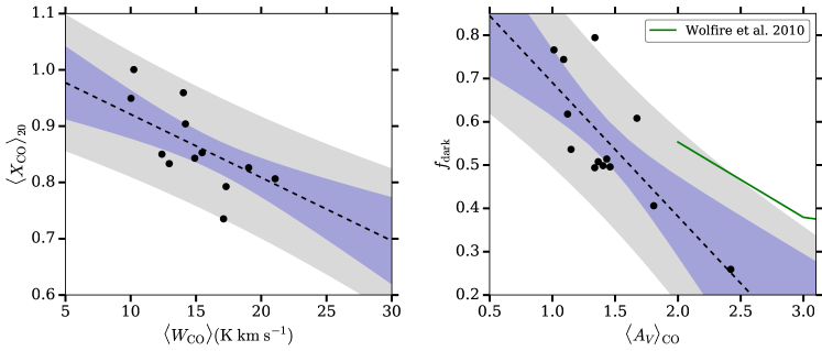
Figure 18.— $\langle X_{\mathrm{CO}}\rangle$ vs. $\langle W_{\mathrm{CO}}\rangle$ (left), and $f_{\mathrm{dark}}$ vs. $\langle A_{V}\rangle_{\mathrm{CO}}$ (right) in models T-356Myr – T-416Myr. The dashed lines are the linear fits to the simulation data (see text). The 90% confidence and prediction intervals from linear regression are indicated by the purple and gray regions. In the right panel, the green line shows the theoretical model of spherical molecular clouds in Wolfire et al. (2010) (their Figure 11, with their definition of $\mathrm{CO}$-dark $\mathrm{H_{2}}$ translated to our definition of $f_{\mathrm{dark}}$ according to Equation (A6)).

Another comparison of $X_{\mathrm{CO}}$ with observations is shown in Figure 19, where the $X_{\mathrm{CO}}$ in each pixel is plotted against $T_{\mathrm{line}}$. Comparing to the California cloud observed by Kong et al. (2015), our simulations shows a similar slope for the relation between $X_{\mathrm{CO}}$ and $T_{\mathrm{line}}$ at $T_{\mathrm{line}}>6~{}\mathrm{K}$ (the observational data are not available at lower $T_{\mathrm{line}}$). However, the value of $X_{\mathrm{CO}}$ at a given $T_{\mathrm{line}}$ is about a factor of $\sim 4$ lower than the observations. One reason for this discrepancy may be that Kong et al. (2015) observed $\mathrm{CO}(J=2-1)$ line and assumed a fixed line ratio of $W_{\mathrm{CO}}(J=2-1)/W_{\mathrm{CO}}(J=1-0)=0.7$, and this ratio is very uncertain. As discussed below in more detail, generally different observations and also our simulations show similar trends for the variations in $X_{\mathrm{CO}}$, but the absolute value of $X_{\mathrm{CO}}$ can differ by a factor of a few.

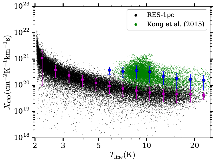
Figure 19.— Scatter plot of $X_{\mathrm{CO}}$ vs. $T_{\mathrm{line}}$ in models T-356Myr – T-416Myr (black) and Kong et al. (2015) (green). Each point is one pixel in the simulations/observations. The red and blue filled circles with error bars are the binned mean values and standard deviations of $X_{\mathrm{CO}}$ in our simulations and Kong et al. (2015).

Using all of the simulation models, a summary of $X_{\mathrm{CO}}$ as a function of $A_{V}(N_{\mathrm{H_{2}}})$ and comparison with observations is shown in Figure 20. Because of the large uncertainties in observations of $X_{\mathrm{CO}}$ at low $A_{V}(N_{\mathrm{H_{2}}})$, we only plot the data at $A_{V}(N_{\mathrm{H_{2}}})>1$. Both in our simulations and the observations, there is a factor of $\sim 2$ variation in $X_{\mathrm{CO}}$ over $A_{V}(N_{\mathrm{H_{2}}})=1-12$. Simulations with $t_{\mathrm{chem}}=50~{}\mathrm{Myr}$ (RES-1pc, RES-2pc, T-356Myr – T-416Myr) show a decrease of $X_{\mathrm{CO}}$ at $A_{V}(N_{\mathrm{H_{2}}})\lesssim 3$, regardless of the resolution and variations in galactic environments. Similar trends can be seen in the observations of Orion molecular clouds by Lee et al. (2018) and Ripple et al. (2013). In contrast, the TCHEM-5Myr model shows a flatter profile at $A_{V}(N_{\mathrm{H_{2}}})\lesssim 3$ and a slight increase of $X_{\mathrm{CO}}$ at $A_{V}(N_{\mathrm{H_{2}}})>3$. Interestingly, the California cloud observed by Lee et al. (2018) also shows a similar trend. Compared to Orion, the California cloud has similar mass and distance, but an order of magnitude lower star formation rate, and therefore is believed to be much younger (Lada et al. 2009). This has interesting implications that the profile of $X_{\mathrm{CO}}$ as a function of $A_{V}(N_{\mathrm{H_{2}}})$ may be used as an indicator of the age of molecular clouds.

Although the trend for the correlation between $X_{\mathrm{CO}}$ and $A_{V}(N_{\mathrm{H_{2}}})$ is similar in our simulations and observations, there is a discrepancy in the absolute value of $X_{\mathrm{CO}}$. This may be due to systematic errors in either observations or simulations. One major uncertainty in observations of $X_{\mathrm{CO}}$ comes from the assumptions in deriving $N_{\mathrm{H_{2}}}$. Estimations of $\mathrm{H_{2}}$ based on $\gamma$-ray emission systematically give a factor of $~{}2$ lower $X_{\mathrm{CO}}$ than dust-based methods, consistent with the value of $X_{\mathrm{CO}}$ in this paper (Bolatto et al. 2013; Remy et al. 2017, see also Figure 20). Even within the dust-based methods, the estimate of $X_{\mathrm{CO}}$ in Orion A based on dust emission is a factor of $\sim 2$ higher in observations of Lee et al. (2018) compared to that in Ripple et al. (2013) based on dust extinction. As another example, the $X_{\mathrm{CO}}$ in Perseus measured by Lee et al. (2014b) (dust emission) is a factor of $\sim 7$ lower than that in Pineda et al. (2008) (dust extinction).

Several possible factors can contribute to the systematics in dust-based observations: different assumptions of the dust to gas ratio, uncertainties in foreground/background subtraction, and different resolutions/beam size (although the resolution effect is relatively mild, as noted by Lee et al. (2014b) and discussed in Section 3.4). Lee et al. (2014b) discussed in detail for the case of Perseus molecular cloud, that all these factors can indeed lead to a different estimate of $X_{\mathrm{CO}}$. Sample differences in observations may also play a role. Most observations of $X_{\mathrm{CO}}$ are for nearby low-mass star forming regions, while most molecular clouds in the Milky Way and our simulations are forming or close to high-mass stars. The feedback form high-mass stars may lead to slightly higher velocity dispersions, and lower $X_{\mathrm{CO}}$. The only nearby high-mass star forming molecular cloud is Orion, and it does have a lower value of $X_{\mathrm{CO}}$ compared to the Milky Way average (Figures 13 and 20).

For the numerical simulations, the main uncertainties lie in the assumptions of equilibrium chemistry and the sub-grid model of micro-turbulence in calculating the $\mathrm{CO}$ emission. As a further test, we produced synthetic observations of model RES-2pc with half of the fiducial micro-turbulence velocity and no sub-grid micro-turbulence (only thermal line-broadening on the grid scale), and found that the values of $X_{\mathrm{CO}}$ increase by a factor of 1.4 and 1.8. Therefore, the uncertainty in sub-grid micro-turbulence may account for part but not all of the discrepencies in $X_{\mathrm{CO}}$ between our simulations and observations. Future AMR simulations with higher numerical resolution and non-equilibrium chemistry will be able to provide more insight into these issues.

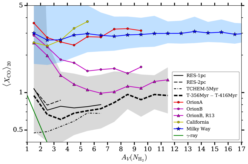
Figure 20.— The average $X_{\mathrm{CO}}$ binned in $A_{V}(N_{\mathrm{H_{2}}})$. The black lines are the simulation models of RES-1pc (solid), RES-2pc (thin dashed), TCHEM-5Myr (dash dotted), and T-356Myr – T-416Myr (thick dashed, 1-$\sigma$ dispersions showing as the gray shaded region). The filled circles show the observations of molecular clouds in Lee et al. (2018) for California (yellow), Orion A (red), and Orion B (magenta). The blue stars show the line-of-sight average of all clouds in Lee et al. (2018) (1-$\sigma$ dispersions showing as blue the shaded region). The magenta triangles show the observations of Orion A by Ripple et al. (2013). The green solid line plots the $\gamma$-ray observations averaged over individual molecular clouds in Remy et al. (2017).

3.4. Dependence of $X_{\mathrm{CO}}$ on the Observational Beam Size

Observation of molecular clouds often have different physical beam sizes/resolutions, which depend on the telescope as well as the distance of the object. In order to investigate the effect of observational resolution on $X_{\mathrm{CO}}$, we smooth the synthetic observations to different beam sizes as described in Section 2.4.

$\langle X_{\mathrm{CO}}\rangle$ increases by a factor of $\sim 2$ as the beam size increases from $\sim 1~{}\mathrm{pc}$ to $\sim 100~{}\mathrm{pc}$, as shown in Figure 21. This is a result of the $\mathrm{CO}$-dark $\mathrm{H_{2}}$. The total $\mathrm{CO}$ emission remains the same as the beam size increases, because the detection limits for different beam sizes (Table 2) are generally sensitive enough to detect most of the $\mathrm{CO}$ emission. This is not surprising as the sensitivity in observations are designed to serve the purpose of accurately measuring the $\mathrm{CO}$ emission. However, the $\mathrm{CO}$ emission is smoothed out spatially as the beam size increases, resulting in a larger area of $\mathrm{CO}$-bright regions. Although the total mass of $\mathrm{H_{2}}$ remains the same, because $X_{\mathrm{CO}}$ is calculated only within $\mathrm{CO}$-bright regions, a larger area of $\mathrm{CO}$-bright regions leads to a larger fraction of $\mathrm{H_{2}}$ mass accounted for, and therefore an increase of $X_{\mathrm{CO}}$. This is clearly illustrated in Figure 22, showing the correlation between $f_{\mathrm{dark}}$ and $\langle X_{\mathrm{CO}}\rangle$. From beam sizes of $\sim 100~{}\mathrm{pc}$ to $\sim 1~{}\mathrm{kpc}$, some simulations show a continued increase of $X_{\mathrm{CO}}$ (e.g. T-401Myr), but some simulations with more diffuse molecular clouds (e.g. T-381Myr) start to have part or all of their $\mathrm{CO}$ emission falling below the detection limits, leading to a non-detection of $W_{\mathrm{CO}}$ or reduction of $X_{\mathrm{CO}}$. This suggests that some diffuse molecular clouds may not be detected with a beam size coarser than $\sim 100~{}\mathrm{pc}$ in extragalactic observations.

In Figure 21, we plot the observations of $\langle X_{\mathrm{CO}}\rangle$ in Milky Way molecular clouds and nearby galaxies (Table 1). Because of the large uncertainties in the observations (as discussed above, and also seen directly in the different $\langle X_{\mathrm{CO}}\rangle$ from two Perseus observations) and dispersions of $\langle X_{\mathrm{CO}}\rangle$ in different molecular clouds, we cannot identify any obvious trend for the $X_{\mathrm{CO}}$ variation with beam size. The general range of $X_{\mathrm{CO}}$ in the simulations is similar to the observations.

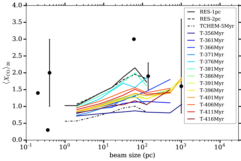
Figure 21.— $\langle X_{\mathrm{CO}}\rangle_{20}$ as a function of beam size in different models (see label). The black circles (with error bars) are observations from Table 1.

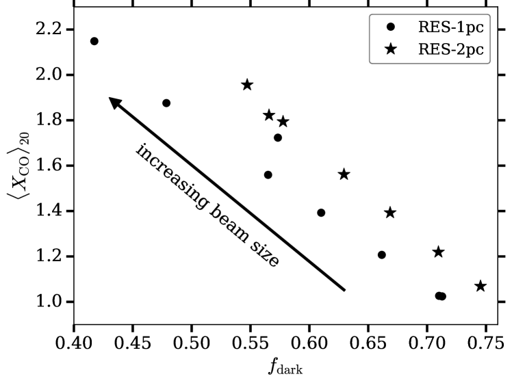
Figure 22.— $\langle X_{\mathrm{CO}}\rangle_{20}$ vs. $f_{\mathrm{dark}}$ in models RES-1pc and RES-2pc. Each point is for a different beam size in Figure 21.

4. Summary

In this paper, we theoretically model the $X_{\mathrm{CO}}$ conversion factor by post-processing MHD galactic disk ISM simulations with chemistry and radiation transfer to produce synthetic observations of molecular clouds. We conduct detailed analyses of the dependence of molecular abundances and observed line strengths on ISM conditions, and also consider numerical and observational effects on calculated and measured $X_{\mathrm{CO}}$. Our main findings are as follows:

1. $\mathrm{CO}$ is only a very approximate tracer of $\mathrm{H_{2}}$. In our simulations, most $\mathrm{H_{2}}$ forms at intermediate densities $n\approx 10-100~{}\mathrm{cm^{-3}}$, but most $\mathrm{CO}$ forms at higher densities $n\gtrsim 200~{}\mathrm{cm^{-3}}$ (Figure 3). The $\mathrm{H_{2}}$ abundance is determined mostly by density, while the $\mathrm{CO}$ abundance by dust shielding (Figures 4, 5). With a $2~{}\mathrm{pc}$ numerical resolution, $\mathrm{H_{2}}$ abundance is converged, but $\mathrm{CO}$ is not. Although there is considerable scatter, the mean relation between the $\mathrm{CO}$ and $\mathrm{H_{2}}$ column densities in the simulations are in agreement with observations of UV absorption spectra (Figure 7).

2. For $\mathrm{CO}$ emission, the high optical depth of the line further complicates the observable relation to $\mathrm{H_{2}}$. On parsec scales, $W_{\mathrm{CO}}$ is largely determined by the mean excitation temperature of $\mathrm{CO}$ (Figure 8), which is in turn determined by the mean gas density. Thus, $W_{\mathrm{CO}}$ most directly probes the mean gas density along the line of sight. However, for the turbulent clouds in our simulations, the mass-weighted mean volume density along a line of sight tends to be correlated with column density. This leads to a correlation between $W_{\mathrm{CO}}$ and $N_{\mathrm{H_{2}}}$ (Figure 11).

3. A numerical resolution of at least $2~{}\mathrm{pc}$ is needed in order to resolve the average $X_{\mathrm{CO}}$ in molecular clouds for solar neighborhood conditions (Figure 12). In our simulations with environmental conditions similar to the solar neighborhood, we found $\langle X_{\mathrm{CO}}\rangle=0.7-1.0\times 10^{20}~{}\mathrm{cm^{-2}K^{-1}km^{-1}s}$, about a factor of 2 lower than the estimate from dust-based observations, and consistent with the $X_{\mathrm{CO}}$ from $\gamma$-ray observations. The value of $\langle X_{\mathrm{CO}}\rangle$ is not sensitive to the variations in molecular cloud mass, extinction, or the strength of the FUV radiation field (Table 5).

4. We found the $\mathrm{CO}$-dark $\mathrm{H_{2}}$ fraction $f_{\mathrm{dark}}=26-79\%$, which has an anti-correlation with the average extinction of molecular clouds (Figure 18 right panel).

5. The chemical timescale for $\mathrm{H_{2}}$ abundance to reach equilibrium is longer than that for $\mathrm{CO}$ (Figure 14), because of differences in characteristic densities. As a result, younger molecular clouds are expected to have lower $\langle X_{\mathrm{CO}}\rangle$ values and flatter profiles of $X_{\mathrm{CO}}$ versus extinction compared to older molecular clouds (Figures 16, 20).

6. As the observational beam size increases from $\sim 1~{}\mathrm{pc}$ to $\sim 100~{}\mathrm{pc}$, $\langle X_{\mathrm{CO}}\rangle$ increases by a factor of $\sim 2$, due to the decrease of the $\mathrm{CO}$-dark $\mathrm{H_{2}}$ fraction (Figures 21, 22).

7. Our numerical simulations successfully reproduce the observed variations of $W_{\mathrm{CO}}$ on parsec scales, as well as the trends for the dependence of $X_{\mathrm{CO}}$ on extinction and the $\mathrm{CO}$ excitation temperature. However, the value of $X_{\mathrm{CO}}$ in our simulations is systematically lower by a factor of $\sim 2$ compared to dust-based observations (Figures 13, 19, 20).

The overall agreement between our numerical simulations and observations of Milky Way molecular clouds give us confidence that similar simulations can be used to probe the $X_{\mathrm{CO}}$ conversion factors in different environments, such as the Galactic center, low metallicity dwarfs, and extreme star-forming systems (ultra luminous infrared galaxies and high redshift galaxies). In a follow-up study, we will investigate the properties of individual molecular clouds in our simulations. In the future, we also plan to integrate full non-equilibrium chemistry with the MHD simulations.

5. Acknowledgment

This work was supported by grants NNX14AB49G from NASA, and AST-1312006 and AST-1713949 from the NSF. We thank the referee for helping us to improve the overall quality of this paper, Jim Stone, Kengo Tomida and Christopher J. White for making the code Athena++ available and their help in developing the chemistry module in the code, Mark H. Heyer for providing the observational data from Ripple et al. (2013), Adam K. Leroy for providing the data from Lee et al. (2018) and helpful discussions of comparisons with observations, Shuo Kong for providing the data from Kong et al. (2015), and Simon C. O. Glover for suggesting an investigation in the effects of the numerical resolution.

Appendix A Definitions of $\mathrm{CO}$-dark $\mathrm{H_{2}}$

In this paper, we define the $\mathrm{CO}$-dark $\mathrm{H_{2}}$ as the molecular gas without $\mathrm{CO}$ emission along a given line of sight. Wolfire et al. (2010) uses a slightly different definition in their spherical cloud model, and they refer the $\mathrm{CO}$-dark $\mathrm{H_{2}}$ as the molecular gas outside of the optical depth $\tau_{\mathrm{CO}}=1$ surface. Their definition of $\mathrm{CO}$-dark $\mathrm{H_{2}}$ includes the $\mathrm{H_{2}}$ along the line of sight in the projected $\mathrm{CO}$-bright areas on the plane of the sky, as long as it is outside of the $\tau_{\mathrm{CO}}=1$ surface (see their Figure 1). In other words, the definition of Wolfire et al. (2010) is in 3D physical space while our definition is in 2D observational space.

To compare the result from Wolfire et al. (2010) to our simulations, we need to translate their definition of $\mathrm{CO}$-dark $\mathrm{H_{2}}$ fraction, denoted by $f_{\mathrm{DG}}$ (their Equation 1) to our definition denoted by $f_{\mathrm{dark}}$ (Equation (10) in this paper). Below we derive the relation between $f_{\mathrm{DG}}$ and $f_{\mathrm{dark}}$. We refer the readers to Figure 1 in Wolfire et al. (2010) for a useful illustration for this derivation.

From Equation (10), $f_{\mathrm{dark}}$ can be written as:

$$f_{\mathrm{dark}}=\frac{M_{\mathrm{H_{2}}}-M_{\mathrm{br}}}{M_{\mathrm{H_{2}}}}=1-\frac{M_{\mathrm{br}}}{M_{\mathrm{H_{2}}}},$$ (A1)

where $M_{\mathrm{H_{2}}}$ is the total $\mathrm{H_{2}}$ mass (same as $M_{\mathrm{H_{2},tot}}$ in Equation (10)), $M_{\mathrm{br}}$ is the mass in $\mathrm{CO}$-bright areas on the projected sky. From Figure 1 in Wolfire et al. (2010), $M_{\mathrm{br}}=M_{\mathrm{CO}}+M_{\mathrm{DG}}$, where $M_{\mathrm{CO}}$ is the mass with $r<R_{\mathrm{CO}}$, and $R_{\mathrm{CO}}$ is the radius of the cloud where $\tau_{\mathrm{CO}}=1$. $M_{\mathrm{DG}}$ is the mass that lies within $R_{\mathrm{CO}}$ in the 2D projected sky, but outside $R_{\mathrm{CO}}$ in the 3D cloud. Compared to the definition in Wolfire et al. (2010),

$$f_{\mathrm{DG}}=1-\frac{M_{\mathrm{CO}}}{M_{\mathrm{H_{2}}}},$$ (A2)

$M_{\mathrm{DG}}$ is the part of the cloud that Wolfire et al. (2010) considered to be $\mathrm{CO}$-dark, but we do not.

Wolfire et al. (2010) assumes the cloud has a density profile $n(r)=n_{0}(r_{0}/r)$, where $n_{0}$ and $r_{0}$ are constants. This gives:

$$M_{\mathrm{H_{2}}}=\int_{0}^{R_{\mathrm{H_{2}}}}4\pi m_{\mathrm{H}}nr^{2}\mathrm{d}r=2\pi n_{0}m_{\mathrm{H}}r_{0}R_{\mathrm{H_{2}}}^{2},$$ (A3)

and similarly,

$$M_{\mathrm{CO}}=2\pi n_{0}m_{\mathrm{H}}r_{0}R_{\mathrm{CO}}^{2},$$ (A4)

where $m_{\mathrm{H}}$ is the mass of the hydrogen atom. $M_{\mathrm{DG}}$ can be estimated by $M_{\mathrm{DG}}\approx 2\pi R_{\mathrm{CO}}^{2}\Sigma_{\mathrm{DG}}$, where $\Sigma_{\mathrm{DG}}=m_{\mathrm{H}}\int_{R_{\mathrm{CO}}}^{R_{\mathrm{H_{2}}}}n\mathrm{d}r=n_{0}m_{\mathrm{H}}r_{0}\ln(R_{\mathrm{H_{2}}}/R_{\mathrm{CO}})$. Therefore,

$$M_{\mathrm{br}}=M_{\mathrm{CO}}+M_{\mathrm{DG}}\approx 2\pi n_{0}m_{\mathrm{H}}r_{0}R_{\mathrm{CO}}^{2}\left[1+\ln\left(\frac{R_{\mathrm{H_{2}}}}{R_{\mathrm{CO}}}\right)\right].$$ (A5)

Equations (A1) – (A5) then gives the relation between $f_{\mathrm{DG}}$ and $f_{\mathrm{dark}}$:

$$f_{\mathrm{dark}}\approx f_{\mathrm{DG}}-\frac{1}{2}(1-f_{\mathrm{DG}})\ln\left(\frac{1}{1-f_{\mathrm{DG}}}\right).$$ (A6)

Appendix B Test of the RADMC-3D code

Figure 23 shows a test for the RADMC-3D radiation transfer code. The level populations of $\mathrm{CO}$ are solved with only the first two rotational levels instead of the default 41 levels. The analytical model uses Equations (27) and (28) to compute $T_{\mathrm{exc}}$ versus $n$. Note that because $\tau_{\mathrm{LVG}}$ depends on level populations (see Equation (7)), the average values of $\tau_{\mathrm{LVG}}$ in this case are slightly larger than that given by Equation (26).

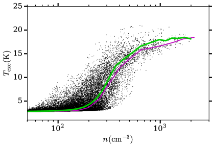
Figure 23.— Comparison of the excitation temperature from the RADMC-3D radiation transfer code (scatter points with median values in density bins shown as the magenta line) to the analytical 2-level system model (green line) for the simulation RES-1pc. Only the $J=0$ and $J=1$ rotational levels of $\mathrm{CO}$ are included in the calculations using RADMC-3D.

References

- Ackermann et al. (2012) Ackermann, M., Ajello, M., Atwood, W. B., et al. 2012, ApJ, 750, 3
- Blitz et al. (1985) Blitz, L., Bloemen, J. B. G. M., Hermsen, W., & Bania, T. M. 1985, A&A, 143, 267
- Bolatto et al. (2013) Bolatto, A. D., Wolfire, M., & Leroy, A. K. 2013, ARA&A, 51, 207
- Burgh et al. (2010) Burgh, E. B., France, K., & Jenkins, E. B. 2010, ApJ, 708, 334
- Crenny & Federman (2004) Crenny, T., & Federman, S. R. 2004, ApJ, 605, 278
- Dame et al. (2001) Dame, T. M., Hartmann, D., & Thaddeus, P. 2001, ApJ, 547, 792
- Downes & Solomon (1998) Downes, D., & Solomon, P. M. 1998, ApJ, 507, 615
- Draine (1978) Draine, B. T. 1978, ApJS, 36, 595
- Draine (2011) —. 2011, Physics of the Interstellar and Intergalactic Medium
- Duarte-Cabral et al. (2015) Duarte-Cabral, A., Acreman, D. M., Dobbs, C. L., et al. 2015, MNRAS, 447, 2144
- Dullemond et al. (2012) Dullemond, C. P., Juhasz, A., Pohl, A., et al. 2012, RADMC-3D: A multi-purpose radiative transfer tool, Astrophysics Source Code Library, ascl:1202.015
- Feldmann et al. (2012) Feldmann, R., Gnedin, N. Y., & Kravtsov, A. V. 2012, ApJ, 758, 127
- Flower (2001) Flower, D. R. 2001, Journal of Physics B: Atomic, Molecular and Optical Physics, 34, 2731
- Flower & Launay (1985) Flower, D. R., & Launay, J. M. 1985, MNRAS, 214, 271
- Glover & Clark (2012) Glover, S. C. O., & Clark, P. C. 2012, MNRAS, 421, 9
- Glover & Mac Low (2007) Glover, S. C. O., & Mac Low, M.-M. 2007, ApJS, 169, 239
- Glover & Mac Low (2011) —. 2011, MNRAS, 412, 337
- Gong & Ostriker (2013) Gong, H., & Ostriker, E. C. 2013, ApJS, 204, 8
- Gong et al. (2017) Gong, M., Ostriker, E. C., & Wolfire, M. G. 2017, ApJ, 843, 38
- Heyer & Dame (2015) Heyer, M., & Dame, T. M. 2015, ARA&A, 53, 583
- Heyer & Brunt (2004) Heyer, M. H., & Brunt, C. M. 2004, ApJ, 615, L45
- Imara (2015) Imara, N. 2015, ApJ, 803, 38
- Israel (1997) Israel, F. P. 1997, A&A, 328, 471
- Kim & Ostriker (2017) Kim, C.-G., & Ostriker, E. C. 2017, ApJ, 846, 133
- Kong et al. (2015) Kong, S., Lada, C. J., Lada, E. A., et al. 2015, ApJ, 805, 58
- Koyama & Inutsuka (2002) Koyama, H., & Inutsuka, S.-i. 2002, ApJ, 564, L97
- Lada et al. (2009) Lada, C. J., Lombardi, M., & Alves, J. F. 2009, ApJ, 703, 52
- Larson (1969) Larson, R. B. 1969, MNRAS, 145, 271
- Larson (1981) —. 1981, MNRAS, 194, 809
- Lee et al. (2018) Lee, C., Leroy, A. K., Bolatto, A. D., et al. 2018, MNRAS, 474, 4672
- Lee et al. (2014a) Lee, E. J., Chang, P., & Murray, N. 2014a, ArXiv e-prints, arXiv:1406.4148
- Lee et al. (2014b) Lee, M.-Y., Stanimirović, S., Wolfire, M. G., et al. 2014b, ApJ, 784, 80
- Leitherer et al. (1999) Leitherer, C., Schaerer, D., Goldader, J. D., et al. 1999, ApJS, 123, 3
- Leroy et al. (2011) Leroy, A. K., Bolatto, A., Gordon, K., et al. 2011, ApJ, 737, 12
- Leroy et al. (2016) Leroy, A. K., Hughes, A., Schruba, A., et al. 2016, ApJ, 831, 16
- Lombardi et al. (2006) Lombardi, M., Alves, J., & Lada, C. J. 2006, A&A, 454, 781
- Narayanan et al. (2011) Narayanan, D., Krumholz, M., Ostriker, E. C., & Hernquist, L. 2011, MNRAS, 418, 664
- Narayanan et al. (2012) Narayanan, D., Krumholz, M. R., Ostriker, E. C., & Hernquist, L. 2012, MNRAS, 421, 3127
- Nelson & Langer (1997) Nelson, R. P., & Langer, W. D. 1997, ApJ, 482, 796
- Nelson & Langer (1999) —. 1999, ApJ, 524, 923
- Penston (1969) Penston, M. V. 1969, MNRAS, 144, 425
- Pineda et al. (2008) Pineda, J. E., Caselli, P., & Goodman, A. A. 2008, ApJ, 679, 481
- Pineda et al. (2010) Pineda, J. L., Goldsmith, P. F., Chapman, N., et al. 2010, ApJ, 721, 686
- Rachford et al. (2002) Rachford, B. L., Snow, T. P., Tumlinson, J., et al. 2002, ApJ, 577, 221
- Remy et al. (2017) Remy, Q., Grenier, I. A., Marshall, D. J., & Casandjian, J. M. 2017, A&A, 601, A78
- Ridge et al. (2006) Ridge, N. A., Di Francesco, J., Kirk, H., et al. 2006, AJ, 131, 2921
- Ripple et al. (2013) Ripple, F., Heyer, M. H., Gutermuth, R., Snell, R. L., & Brunt, C. M. 2013, MNRAS, 431, 1296
- Safranek-Shrader et al. (2017) Safranek-Shrader, C., Krumholz, M. R., Kim, C.-G., et al. 2017, MNRAS, 465, 885
- Sandstrom et al. (2013) Sandstrom, K. M., Leroy, A. K., Walter, F., et al. 2013, ApJ, 777, 5
- Schlafly et al. (2014) Schlafly, E. F., Green, G., Finkbeiner, D. P., et al. 2014, ApJ, 786, 29
- Seifried et al. (2017) Seifried, D., Walch, S., Girichidis, P., et al. 2017, ArXiv e-prints, arXiv:1704.06487
- Sheffer et al. (2008) Sheffer, Y., Rogers, M., Federman, S. R., et al. 2008, ApJ, 687, 1075
- Shetty et al. (2011a) Shetty, R., Glover, S. C., Dullemond, C. P., & Klessen, R. S. 2011a, MNRAS, 412, 1686
- Shetty et al. (2011b) Shetty, R., Glover, S. C., Dullemond, C. P., et al. 2011b, MNRAS, 415, 3253
- Smith et al. (2012) Smith, M. W. L., Eales, S. A., Gomez, H. L., et al. 2012, ApJ, 756, 40
- Solomon et al. (1987) Solomon, P. M., Rivolo, A. R., Barrett, J., & Yahil, A. 1987, ApJ, 319, 730
- Stone & Gardiner (2010) Stone, J. M., & Gardiner, T. A. 2010, ApJS, 189, 142
- Stone et al. (2008) Stone, J. M., Gardiner, T. A., Teuben, P., Hawley, J. F., & Simon, J. B. 2008, ApJS, 178, 137
- Strong & Mattox (1996) Strong, A. W., & Mattox, J. R. 1996, A&A, 308, L21
- Sutherland & Dopita (1993) Sutherland, R. S., & Dopita, M. A. 1993, ApJS, 88, 253
- Szűcs et al. (2016) Szűcs, L., Glover, S. C. O., & Klessen, R. S. 2016, MNRAS, 460, 82
- White et al. (2016) White, C. J., Stone, J. M., & Gammie, C. F. 2016, ApJS, 225, 22
- Wolfire et al. (2010) Wolfire, M. G., Hollenbach, D., & McKee, C. F. 2010, ApJ, 716, 1191
- Wolfire et al. (1993) Wolfire, M. G., Hollenbach, D., & Tielens, A. G. G. M. 1993, ApJ, 402, 195