Variability search in M 31 using Principal Component Analysis and the Hubble Source Catalog

Abstract

Principal Component Analysis (PCA) is being extensively used in Astronomy but not yet exhaustively exploited for variability search. The aim of this work is to investigate the effectiveness of using the PCA as a method to search for variable stars in large photometric data sets. We apply PCA to variability indices computed for light curves of 18152 stars in three fields in M 31 extracted from the Hubble Source Catalogue. The projection of the data into the principal components is used as a stellar variability detection and classification tool, capable of distinguishing between RR Lyrae stars, long period variables (LPVs) and non-variables. This projection recovered more than 90% of the known variables and revealed 38 previously unknown variable stars (about 30% more), all LPVs except for one object of uncertain variability type. We conclude that this methodology can indeed successfully identify candidate variable stars.

1 Introduction

An increasing number of time-domain surveys are producing large catalogs of multi-epoch and multi-band photometric data, making it ever more important to invent algorithms that efficiently detect and classify variable objects. Multi-epoch photometry from the ground is collected by surveys for optical transients (e.g. Palomar Transient Factory –  PTF, Law et al. 2009; Catalina Real-Time Transient Survey – CRTS, Drake et al. 2009; All Sky Automated Survey for SuperNovae – ASAS-SN, Shappee et al. 2014), microlensing surveys (MAssive Compact Halo Object – MACHO, Griest et al. 1991; Optical Gravitational Lensing Experiment – OGLE, Udalski et al. 2008; Expérience pour la Recherche d’Objects Sombres – EROS, Kim et al. 2014, Tisserand et al. 2007), near-infrared surveys (e.g. Vista Variables in the Via Lactea – VVV, Minniti et al. 2010; The Vista near-infrared $Y$, $J$, $K_{S}$ survey of the Magellanic Clouds – VMC, Cioni et al. 2011), ground-based exoplanet surveys (Trans-Atlantic Exoplanet Survey – TrES, Alonso et al. 2007; Super Wide Angle Search for Planets – SuperWASP, Butters et al. 2010; Hungarian-made Automated Telescope Network – HATNet, Bakos et al. 2004; the Kilodegree Extremely Little Telescope – KELT, Pepper et al. 2007) and from space by Gaia (Perryman et al. 2001, Gaia Collaboration et al. 2016, Clementini et al. 2016) and Kepler (Koch et al. 2010) with the next generation time-domain surveys running or just around the corner ( among them PanSTARRS, Chambers et al. 2016; Large Synoptic Survey Telescope – LSST, Ivezic et al. 2008; the Next Generation Transit Survey – NGTS, Wheatley et al. 2017).

Identifying variable objects in a set of light curves (LCs) is non-trivial as the photometric measurements are often affected by correlated noise and outliers (Sec. 5). Traditional variability detection techniques include: identifying LCs with high scatter (e.g. Kolesnikova et al., 2008; Burdanov et al., 2016; Dutta et al., 2018) or the ones showing smooth systematic variations (Welch & Stetson, 1993; Stetson, 1996; Mowlavi, 2014), periodicity search (Fruth et al., 2012; Drake et al., 2014; Oelkers et al., 2018; Medina et al., 2018) and LC template fitting (Layden et al., 1999; Yoachim et al., 2009; Angeloni et al., 2014; Sesar et al., 2017). It is desirable for a variability detection algorithm to have the capability of detecting not only specific types of variable stars (e.g. Cepheids) or transient events with unique signatures (e.g. microlensing events), but also to discover all variable sources within the capabilities of a given survey. Once a variable object has been detected, it is often desired to determine its variability type from the light curve. Methods for automatically classifying LC of variable stars have been investigated by several authors (Debosscher et al. 2007, Paegert et al. 2014, Kim & Bailer-Jones 2016).

The “Hubble Catalog of Variables” (HCV; Gavras et al. 2017, Sokolovsky et al. 2017b, Yang et al. 2017) is an ESA project aiming to develop an algorithm for automatically detecting all variable sources within the Hubble Source Catalog (HSC, Whitmore et al. 2016) which will populate the HCV. The HSC will ultimately contain photometry of all sources observed by the main cameras on the Hubble Space Telescope (HST) over its lifetime. Despite the fact that HST observations have been extensively used for variability studies (e.g. Freedman et al., 2001; McCommas et al., 2009; Clementini et al., 2009; Fiorentino et al., 2010, 2013; Di Criscienzo et al., 2011; Bernard et al., 2013; Hoffmann et al., 2016) the HSC contains a wealth of variability information that is yet to be explored. While constructing the HCV pipeline we considered a number of statistical characteristics, referred hereafter as variability indices (Sec. 3.1), which quantify LC scatter and/or its smoothness. The ability of each index to identify variable sources depends on the variability type and observing cadence. Since the HST archive includes observations of Galactic and extragalactic fields (expected to have stellar variable sources as well as active galaxies, supernovae etc.) performed with various observing cadence over various time intervals, a single variability index will not optimally find variables in all HST fields. Here we explore a technique that may solve the problem of selecting an optimal variability index by automatically finding a quasi-optimal combination of multiple variability indices with no a priori information about the types of variable objects found in a given field.

Sokolovsky et al. (2017a) have investigated the effectiveness of applying variability indices to ground-based photometry. The authors proposed two robust ways of identifying variable sources in time-series photometry of any cadence: (i) to use a combination of two indices, the correlation-based inverse von Neumann ratio and the scatter-based Interquartile Range and (ii) to use the admixture coefficient of the first principal component resulting from the principal component analysis (PCA), as an optimal linear combination of multiple variability indices. Despite ground-based data are unstable both in terms of detector performance as well as in PSF variability due to seeing, it was found that the variability-related information may be recovered from the first significant principal component, without having to identify which index is the most suitable for each data set in advance.

In the current study we extend the PCA-based methodology of variability detection and apply it to variability indices derived from HSC LC of sources in three fields in M 31. These fields constitute part of the “control sample” for the HCV, as they have been studied in terms of variability by Brown et al. (2004) and Jeffery et al. (2011). Our goal is to construct a nearly-complete list of variable sources in these fields and evaluate the applicability of the PCA-based method to LCs containing a much smaller number of epochs than those investigated by Sokolovsky et al. (2017a). This technique is not specific to the HSC, but can be applied to identify variable sources in virtually any large set of LCs.

This paper is structured as follows: Section 2 describes the data used in this study; Section 3 introduces the PCA-based variability detection method adopted for the analysis; Section 4 presents the newly discovered variables and compares them with previously reported variables in the studied fields. In Section 5 we discuss the results and in Section 6. we summarize the conclusions.

2 Data

2.1 The Hubble Source Catalog

We extract the multi-epoch photometry from the HSC version 1 (HSCv1, Whitmore et al. 2016), which contains 80 million detections of 30 million sources. The catalog is based on images obtained with the WFPC2, ACS/WFC, WFC3/UVIS and WFC3/IR cameras on board the HST over a period of 16, 15, 8 and 8 years, respectively. As the HST data were collected with different instruments, filters and observing strategies, the photometric accuracy, data quality and cadence of observations vary greatly across the HSC, making the detection of variable objects a non-trivial task. The HSCv1 contains about 5 million sources with more than 2 measurements and about 40,000 objects with more than 10 measurements obtained with the ACS/F814W instrument/filter combination. The F814W is available also on the other cameras: WFPC2 and WFC3. The F814W magnitudes of objects listed in HSCv1 range from 15th to 26th mag for WFPC2, 15–27 mag for ACS and 16–28 mag for WFC3. The mean photometric accuracy is better than 0.10 mag, while the relative accuracy is $\simeq$ 0.02 mag at best. HSCv1 is based on the Hubble Legacy Archive (HLA) Data Release 8 images.

A visit is a series of one or more exposures on a target, including overheads, that are executed in one or more consecutive orbits. The exposures are interleaved by the time required for dithering, filter change, other instrumental overheads and the time the target source is occulted by the Earth. All exposures taken within one visit are combined by the HLA into a white-light image that is used for source detection. For each filter used in a given visit, the images taken in this filter are also combined. The filter-combined images are used to measure brightness of the sources in each filter during the visit. These stacked images are used for source extraction and photometry for the purpose of removing image artifacts caused by cosmic ray hits. The SExtractor software (Bertin & Arnouts, 1996) is employed to produce the HLA source lists providing magnitude measurements for each source. SExtractor is operated in dual-image mode with the white-light image used for source detection and filter-combined images used for photometry. Since the HSCv1 photometry is visit-based, the HSCv1 light curves for a specific source typically contain fewer data points compared to the respective LC presented in the literature that are usually extracted from individual images within a visit.

Positions of sources detected on the visit-combined HLA images are based on the information from HST fine guidance sensors. While the fine guidance sensors have superb internal astrometric accuracy (Benedict et al., 2017), the absolute positions reported by them are limited by the position accuracy of individual guide stars. The resulting absolute position errors could be as large as $\sim$1–2 arcsec for HST images obtained before 2005 when the Guide Star Catalog 2 became available (Lasker et al., 2008). The HSC is using PanSTARRS, SDSS (Ahn et al., 2014) and 2MASS (Skrutskie et al., 2006) sources within the HST cameras’ field of view to refine the absolute astrometry of the HLA images. The lists of sources detected during multiple visits of the same sky area are cross-matched using the Bayesian technique proposed by Budavári & Lubow (2012). This results in the final absolute astrometric accuracy of better than 0.1 arcsec for most of the HSC sources (Whitmore et al., 2016).

2.2 M 31 fields

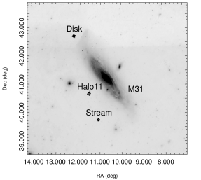
Figure 1: Finder chart of the M 31 Halo11, Disk and Stream fields, from the Digitized Sky Survey. North is up, east is to the left.

We selected three fields in M 31 observed by HST. These HST fields were originally investigated for variability by Brown et al. (2004) and Jeffery et al. (2011). The fields fall on the southeast minor axis (“Halo11”), on the north-east major axis (“Disk”) and in the giant stellar stream of metal rich stars (“Stream”; Ibata et al. 2001; Kirihara et al. 2017), as illustrated in Figure 1. The selection of these fields was based on (i) the large number of published variables (100 RR Lyrae stars and more than 30 Long Period Variables – LPVs) with very good astrometry and (ii) the availability of LC in two filters (F606W and F814W) in the HSCv1. Table 1 summarizes the main characteristics of these fields and the corresponding observations: coordinates, original Program ID, number of HSCv1 sources, minimum, maximum and median number of HST visits (corresponding to the number of data points in the HSCv1 LC) and time (modified Julian date, MJD) and magnitude range. In the Halo11 and the Disk fields $\sim$7000 point sources were detected in HSCv1, while $\sim$4300 sources were recorded in the Stream field. For the Halo11 field, the observations were obtained over a period of 40 days. The corresponding LC contain about twice as many visits as the Stream and Disk LC, which were obtained at lower cadence and over a shorter period of about 30 days (see discussion in Brown et al. 2009).

Table 1: Characteristics of the M 31 fields selected for PCA. In particular, Col. 6 and 7 indicate the number of minimum-maximum, median visits in F606W and F814W filters respectively.

Field	RA (deg)	Dec (deg)	Program ID	HSCv1	# Visits	# Visits	MJD range	MJD range
	J2000	J2000		sources	F606W	F814W	F606W	F814W
Halo11	11.52958	40.71083	GO-9453	7109	6-27, 27	6-33, 33	52610-52650	52611-52650
Disk	12.28583	42.75055	GO-10265	6732	6-11, 11	6-16, 16	53359-53374	53350-53389
Stream	11.07583	39.79222	GO-10265	4311	6-10, 10	6-15, 15	53248-53282	53250-53282

The HSCv1 sources used in our analysis satisfy the following criteria: (i) they are point sources according to the HSCv1 classification flag; (ii) they have at least 6 measurements in both the F606W and F814W LC; (iii) they are located within 240 arcsec from the center of the corresponding field; (iv) they have a SExtractor flag $\leq$7. Sources satisfying this constraint may be affected by bright and nearby neighbors, bad pixels affecting at least 10% of the integrated area, blending with another source, or saturated pixels. We retained data points marked as saturated since in the HSCv1 the saturation level is set incorrectly. Sources within $\sim$ 0.5 mag of the bright limit in either filter (see Table 1) are discarded at a later stage of the analysis to avoid false variability introduced by possible saturation (Section 4). Sources within 0.5 mag of the faint limit in either filter (Table 1) were treated with particular care (Section 4).

With the above constraints, we ended up with a catalog of 18152 sources in the three fields (“HSCv1 based sample” hereafter). Figure 2 shows the normalized magnitude histograms for the three fields. The histograms are similar for each filter in both bands, with a slight exception around magnitudes 24-26 mag, possibly due to different stellar population properties (Brown et al. 2006, 2009; Jeffery et al. 2011; see also discussion in Section 4).

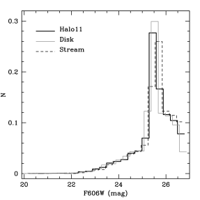
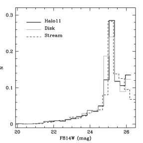
Figure 2: Normalized distribution of the mean F606W and F814W magnitudes of HSC sources in the three fields.

3 Methodology

3.1 Variability indices

We characterize each LC by its mean magnitude and the values for 18 variability indices. For a variable source we expect that (i) its LC has larger scatter than the LC of a non-variable object of similar brightness (irrespective of the variability timescale) and (ii) the measurements taken close in time result in similar magnitudes (i.e. the LC is smooth) if the variability timescale is significantly longer than the LC sampling rate. The variability indices used here capture one or both of these characteristics. In addition to the measured magnitudes, some indices take into account the estimated photometric errors, as well as the order and time at which the measurements were obtained. Table 2 presents the summary of the indices used and whether errors, order of observations or time of observations are taken into account by the corresponding index. A detailed discussion of these indices may be found in Sokolovsky et al. (2017a), see also Ferreira Lopes & Cross (2016a, 2017). While we used an HCV pipeline prototype to compute the variability indices, all the indices listed in Table 2 can also be computed by the freely available VaST code (Sokolovsky & Lebedev, 2018).

Characterizing a LC with variability indices is directly analogous to the feature extraction (Nun et al., 2015; Christ, Kempa-Liehr, & Feindt, 2016) performed

for machine learning classification of variable stars (Debosscher et al., 2009; Richards et al., 2011; Kim & Bailer-Jones, 2016). However, here, we purposefully avoid features based on periodicity in order to have the same set of indices characterizing periodic, irregular and non-variable objects. Period search results may not be reliable given the small number of observing epochs. Typically, more than a hundred brightness measurements that randomly sample the LC are needed for a reliable period determination (Horne & Baliunas 1986, Graham et al. 2013). A method of characterizing LCs without defining variability features is proposed by Kügler, Gianniotis, & Polstere (2015).

Although the individual indices are useful tools for variability search, a combination of multiple indices may be an even better variability indicator, as different indices are sensitive to different types of variability. The PCA offers a promising option to optimally combine variability indices, without having to decide a priori which indices are more suitable for a given data set. The PCA also provides a natural way to combine multi-band data for variability search, as it is possible to add features computed from the LC in all available filters.

Table 2: Variability indices used as an input for the PCA.

Index	Ref.	Errors	Order	Time
Scatter-based indices
reduced $\chi^{2}$ statistic ($\chi_{\rm red}^{2}$)	(a)	$\checkmark$
weighted standard deviation ($\sigma$)	(b)	$\checkmark$
median abs. deviation (${\rm MAD}$)	(c)
interquartile range (${\rm IQR}$)	(d)
robust median statistic (${\rm RoMS}$)	(e)	$\checkmark$
norm. excess variance ($\sigma_{\rm NXS}^{2}$)	(f)	$\checkmark$
norm. peak-to-peak amp. ($v$)	(g)	$\checkmark$
Stetson’s $K$ index	(h)
Correlation-based indices
Stetson’s $J$ index	(h)	$\checkmark$	$\checkmark$	$\checkmark$
weighted Stetson’s $J({\rm time})$ index	(i)	$\checkmark$	$\checkmark$	$\checkmark$
clipped Stetson’s $J({\rm clip})$ index	(d)	$\checkmark$	$\checkmark$	$\checkmark$
Stetson’s $L$ index	(h)	$\checkmark$	$\checkmark$	$\checkmark$
weighted Stetson’s $L({\rm time})$ index	(i)	$\checkmark$	$\checkmark$	$\checkmark$
clipped Stetson’s $L({\rm clip})$ index	(d)	$\checkmark$	$\checkmark$	$\checkmark$
excursions ($E_{x}$)	(j)	$\checkmark$	$\checkmark$	$\checkmark$
autocorrelation ($l_{1}$)	(k)		$\checkmark$
inv. von Neumann ratio ($1/\eta$)	(l)		$\checkmark$
$S_{B}$ statistic	(m)	$\checkmark$	$\checkmark$

References: (a) de Diego (2010), (b) Dutta et al. (2018), (c) Zhang et al. (2016), (d) Sokolovsky et al. (2017a), (e) Rose & Hintz (2007), (f) Nandra et al. (1997), (g) Brown et al. (1989), (h) Stetson (1996), (i) Fruth et al. (2012), (j) Parks et al. (2014), (k) Kim et al. (2011), (l) Shin et al. (2009), (m) Figuera Jaimes et al. (2013).

3.2 Principal Component Analysis

The PCA (Pearson, 1901) is extensively used in Astronomy (e.g. Bailer-Jones et al. 1998, Re Fiorentin et al. 2007, Yip et al. 2004, Karampelas et al. 2012, Steiner et al. 2009). It has also been employed for variable star detection using multi-band LCs (Süveges et al., 2012; Sokolovsky et al., 2017a), as first suggested by Eyer (2006). PCA linearly and orthogonally transforms a data set of $m$ quantities (where each data point is represented by a vector, $\mathbf{x_{j}}$, in the $m$-dimensional space) onto a new set of $m$ uncorrelated axes (the eigenvectors of the variance-covariance matrix of the data), where the data variance is being emphasized. These eigenvectors are called the principal components (PCs). Each observation $\mathbf{x_{j}}$ of the original data is expressed as

$$\mathbf{x_{j}}=\sum_{i=1}^{m}a_{j,i}\cdot\mathbf{PC_{i}}$$ (1)

where $a_{i}$ is the admixture coefficient of the principal component $\mathbf{PC_{i}}$. The coefficients $a_{i}$ are the coordinates of the data point $\mathbf{x_{j}}$ in the new axes.

PCs are ordered so that $\mathbf{PC_{1}}$ accounts for the highest data variance, $\mathbf{PC_{2}}$ (uncorrelated to $\mathbf{PC_{1}}$) incorporates most of the remaining variance and so on. Thus, along the sequence from $\mathbf{PC_{1}}$ to $\mathbf{PC_{m}}$, information, assumed to be represented by the data variance, extends from widespread, to rare, to noise. The amount of the variance corresponding to each PC is the respective eigenvalue $\lambda_{i}$ divided by the sum of all the eigenvalues. This relation originates from the diagonalization of the data variance-covariance matrix $C$, achieved through the PCA implementation. Each element $c_{ij}$ of $C$ is the covariance between the $i$-th and the $j$-th variables. If $i=j$, then $c_{ii}$ is the variance of the $i$-th variable. The variance-covariance matrix $C^{{}^{\prime}}$ of the transformed data is diagonal, having $c_{ij}^{{}^{\prime}}=0$ and $c_{ii}^{{}^{\prime}}=\lambda_{i}$. The larger the $\lambda_{i}$, the higher the variance represented by $\mathbf{PC_{i}}$.

Since the lower-order PCs do not represent any useful information, each observation can be approximately expressed by replacing $m$ with $r$ in Eq. (1) where $r<m$. There is no standard procedure for deciding how many principal components should be kept. If $r=2$ or $r=3$, the data can be visualized in two or three dimensions, using the corresponding admixture coefficients $a_{1}$, $a_{2}$ and $a_{3}$. The resulting dimensionality reduction/data compression is among the advantages of the PCA. The PCA is an unsupervised (no need for training data) and non-parametric (no need for tuning) procedure that provides a linear decomposition. On the other hand, PCA may not perform very well when the processes dominating the original data are not linear, although alternatives do exist such as kernel-PCA (e.g. Ishida & de Souza 2013) and robust-PCA (e.g. de Souza et al. 2014). PCA is also data-dependent, thus requiring a standardization of the original data, if the data variables express different characteristics (Sec. 3.3).

3.3 PCA implemented in the M 31 fields

The input characteristics for the PCA were the 18 variability indices listed in Table 2 and the mean magnitude computed for the LCs in each filter (F606W and F814W), resulting in a total of 38 parameters, for all sources detected in the three selected M 31 fields (Halo11, Disk and Stream). The variability indices were first standardized to zero average and unit variance. Standardization is necessary since the variance-enhancing PCA is data dependent and the input characteristics express different quantities. High values of an index may result in numerically large variance, although this index may not contain useful variability information. The standardized index values express the deviation from the average in multiples of the standard deviation, making the various indices comparable. By construction, large values of the variability indices (subsequently, positive values well above the zero average of the standardized indices) are expected to correspond to variable stars.

The scree plot presented in Figure 3 illustrates the percentage of the total variance that corresponds to the 10 most significant PCs.

High variance is caused by high values of the variability indices of variable sources, thus linking the most significant principal components to variable sources. About 60% of the data variance is captured by the first two PCs (average value for the three fields).

Figure 3: Scree plot representing the variances of the 10 most significant Principal Components.

3.4 Selection of candidate variables

The detectability of variable sources hinges on the following assumptions: (a) The sample contains variables and therefore the variability indices by construction contain variability information from the LC. (b) Variability is mainly encoded in $\mathbf{PC_{1}}$ and $\mathbf{PC_{2}}$ and their respective values (admixture coefficients $a_{1}$ and $a_{2}$.) The high values of the variability indices of the variable stars and their respective high variance “feed” the most significant principal components, since PCA preferentially highlights variance. Therefore, the variability information is expected to be encoded in the most significant principal components. (c) Variable stars are found in sparse regions on the $a_{1}$–$a_{2}$ plane, while constant stars have $a_{1}$ and $a_{2}$ values close to zero. Additionally, the observational fact that the majority of stars appear to be constant (at the level of photometric accuracy expected from HSC), ensures that they will form the distinct dense area in the $a_{1}$–$a_{2}$ plane, making the variables more easily distinguishable. Thus, sparseness in the $a_{1}$–$a_{2}$ plane emerges from variable stars being rare and having wider $a_{1}$ and $a_{2}$ ranges compared to the constant stars.

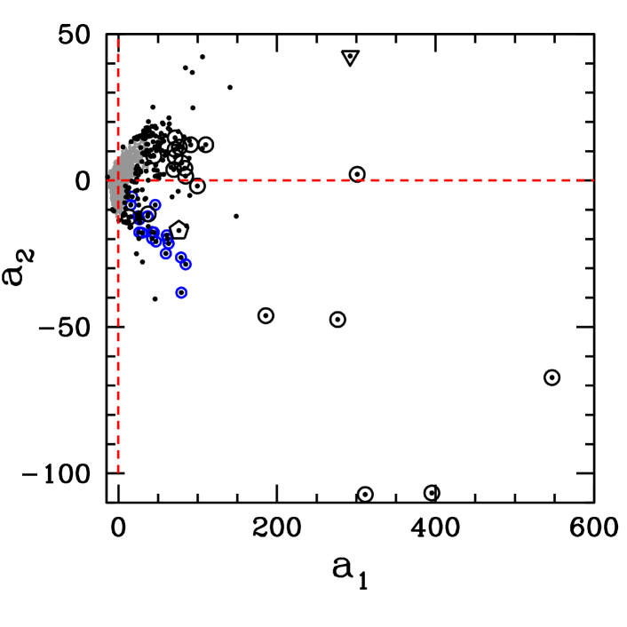
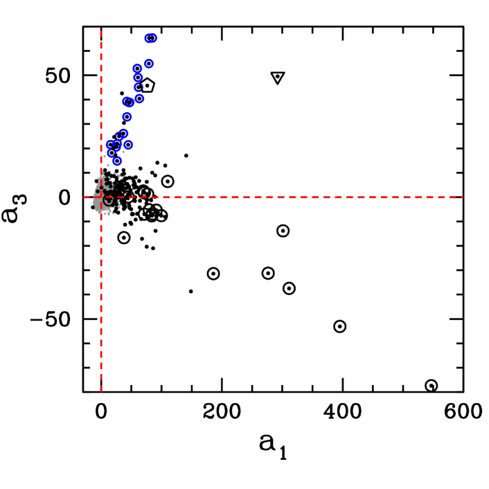
Figure 14: Same as Figure 4, but for the M 31 Disk. The candidate variables obtained with the method described in Section 3.4 are highlighted with black points, while newly discovered variables are marked with big black open circles. Small blue open circles, the black open pentagon and reversed black open triangle highlight RR Lyrae stars, anomalous and classical Cepheid variables, respectively, from Jeffery et al. (2011).

As the first two PCs summarize most of the data variance, we exploit the corresponding admixture coefficients $a_{1}$ and $a_{2}$ to identify variable sources. It is noted that the PCs are global for each field (all stars share the same $\mathbf{PC_{i}}$), while the admixture coefficients are star specific (each star has its own set of $a_{i}$). The upper left panel of Figure 4 shows the distribution of all sources in the Halo11 field on the $a_{1}$–$a_{2}$ plane. The great majority of sources occupy a distinct dense region around zero $a_{1}$ and $a_{2}$ values and are interpreted as “constant” sources. A small number of sources, with high absolute values of $a_{1}$ and $a_{2}$, lie outside this dense locus and are expected to correspond to variable sources. Similar plots for the Stream and Disk fields can be found in the Appendix (top left panel of Figures 14,  15). We employ the following two-step approach to select candidate variables.

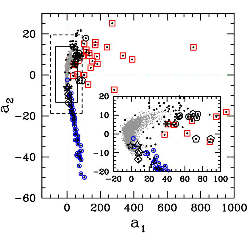
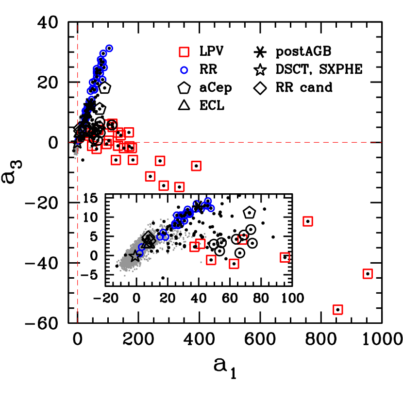
Figure 4: The location of candidate variables (black points) on the admixture coefficient planes for M 31 Halo11. The known LPVs (red open squares), RR Lyrae stars (small blue open circles), RR Lyrae star candidates (black open diamonds), eclipsing binaries (black open triangles), the dwarf Cepheid (black open star), the anomalous Cepheids (black open pentagons), the post-AGB star (black asterisk) are labeled, along with all the sources (grey dots). The newly discovered variables are marked with big black open circles. The solid box corresponds to the initial step of the selection process (step (i) in Sec. 3.4), while the dashed box indicates the region where the second step ((ii) in Sec. 3.4) of the process was applied. Insets present the most crowded areas.

(i) Initial selection of candidate variables
Any star with $a_{1}$ or $a_{2}$ values that differs at least three standard deviations ($3\sigma$) from the corresponding median values (i.e. outside the black solid line box in the upper-left panel of Figure 4), was considered to be a variable star candidate. The $a_{1}$ and $a_{2}$ medians, dominated by the low $a_{1}$ and $a_{2}$ values of the constant stars, would be low as well. The standard deviations, dominated by the extreme $a_{1}$ and $a_{2}$ values of some variable stars, will be relatively high. Thus, this criterion is expected to ensure detection of actual variable stars.

(ii) Selection fine-tuning
Even inside the solid line box of Figure 4 there are sources near but not inside the dense zone of, presumably, constant stars (that is not rectangular in shape). To retrieve these candidates we used the average (Euclidean) $a_{1}$–$a_{2}$ distance of each source inside the solid line box to its three nearest neighbors (hereafter d_k for the $k$-th star), the median source-to-source distance inside the box ($D_{inside}$), and the median source-to-source distance outside the box ($D_{outside}$), in an equal area lying between the solid and the dashed lines of Figure 4.

By construction, $D_{inside}$ characterizes constant stars, as the vast majority of sources inside the box are expected to be non-variables. On the other hand, most of the stars contained in the outer box are expected to be variables. Thus, for the $k$-th inner box star to be a variable candidate, its distance $d_{k}$ is expected to have a value closer to $D_{outside}$ rather than to $D_{inside}$, that is $|d_{k}-D_{outside}|<|d_{k}-D_{inside}|$.

The resulting candidate variables are marked with black dots on the $a_{1}$–$a_{2}$ selection plane for M 31 Halo11 (upper left panel of Figure 4). These candidate variables are validated and compared against published variables in Section 4. The candidate variables are also marked on higher order admixture coefficient planes (remaining panels of  Figure 4) which are further discussed in Section 5.1. Similar plots are available for the Disk and Stream fields in the Appendix (Figures 14,  15).

4 Results

The two step selection procedure described in the previous section, resulted in a total of 156 candidate variables in the Halo11 field (2.2% of the total number of sources), 192 in the Disk field (2.9%) and 88 in the Stream field (2.0%). Figures 5, 6, 7 show the color magnitude diagrams (CMD) for the three fields, respectively. The sources lie on the red giant (RGB), subgiant (SGB), asymptotic giant (AGB) and horizontal branches (HB). In most cases, main sequence stars lie below the detection limit, with the exception of the Disk field where they are detected at $\sim$23rd magnitude, indicating the presence of a younger population (see also Jeffery et al. 2011, Brown et al. 2006, 2009). The location of the candidates on the CMD is also shown (black points in Figures 5, 6, 7). Most of the candidate variables are associated with the HB where one expects to find RR Lyrae stars, with the AGB where one would expect to find LPVs and with the supergiant region. Several candidates lie on the RGB and SGB and might be eclipsing binaries. We consider as reliable variable candidates stars fainter than 21.0 mag in F606W (20.5 in F814W), corresponding to the saturation limit derived from the raw HST images.

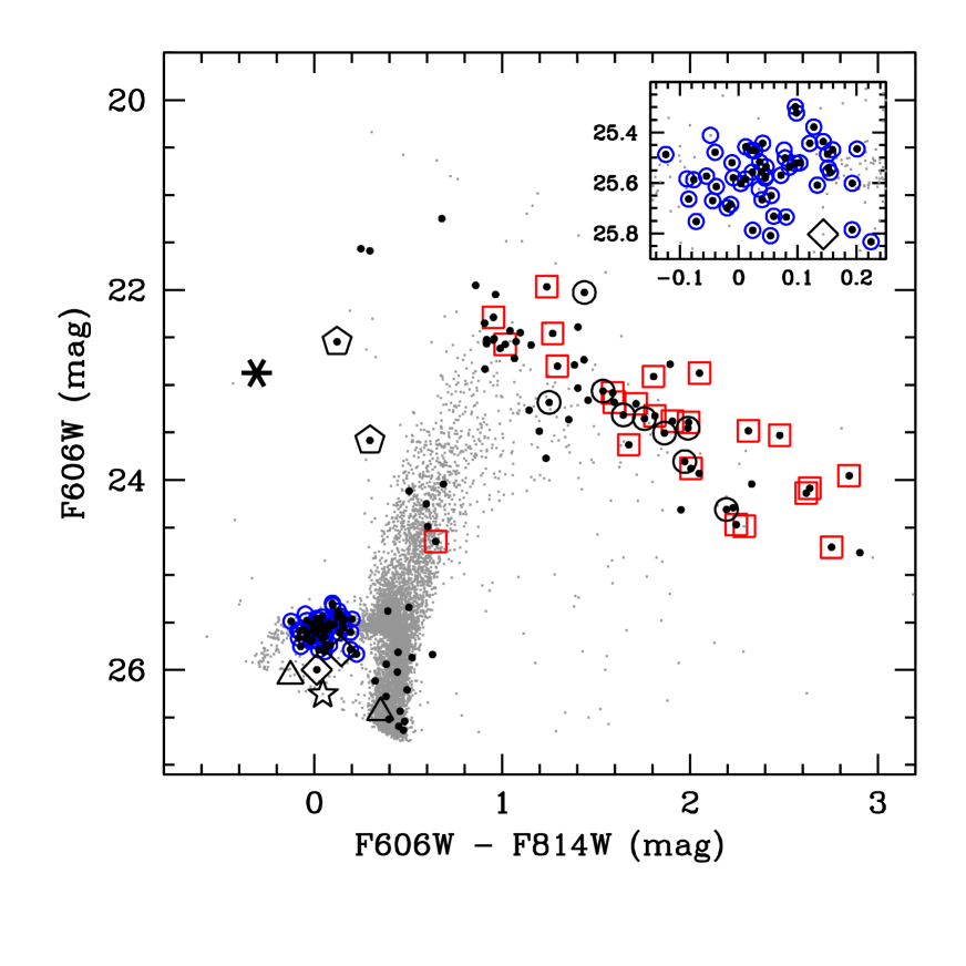
Figure 5: Color-magnitude distribution of sources in the Halo11 field. All sources are represented with grey dots, the PCA variable candidates are shown with black points. The new and known variables are labeled as in Figure 4. The inset presents the HB region.

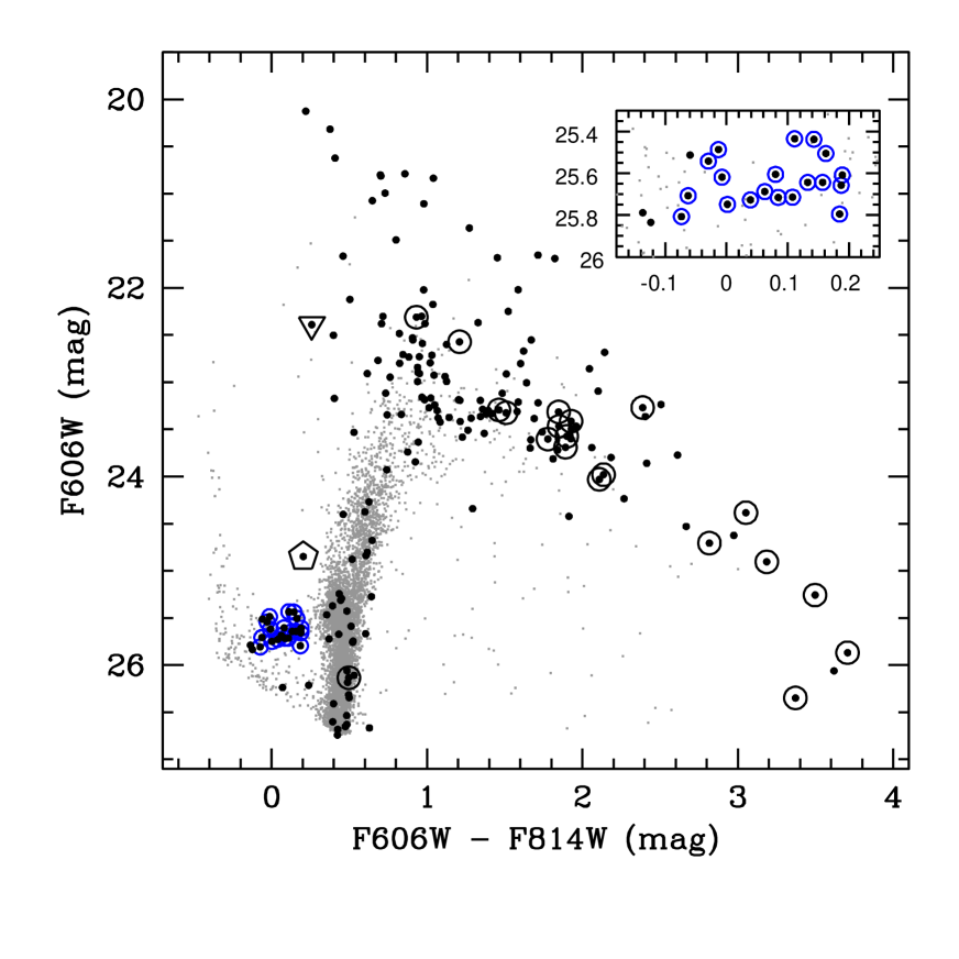
Figure 6: Same as Fig. 5, but for the Disk field. The literature variables are from Jeffery et al. (2011); the classical Cepheid is marked by a reversed open triangle.

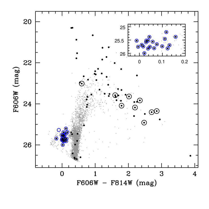
Figure 7: Same as Fig. 5, but for the Stream field. The literature variables are from Jeffery et al. (2011).

4.1 Recovery of known variables

To compare the list of variable stars published by Brown et al. (2004) and Jeffery et al. (2011), to our list of candidate variables (Section 3.4) and evaluate the effectiveness of our variability selection technique, we first need to ascertain whether a published variable is present in the HSCv1 based sample, as defined in 2.2. Some of the published variables may be excluded due to differences in image processing and source extraction strategies used to create the HSC and the ones employed by Brown et al. (2004) and Jeffery et al. (2011). For the same reason some of the sources that could not be used in the original studies may become useful for variability search through the HSC.

Most of the published variables have an HSCv1 counterpart within about 0.6 arcsec, indicating that the published and the HSCv1 astrometry are in good agreement. For RR Lyrae variables the validity of HSCv1 counterparts to the published variables was confirmed by visual inspection of the LC folded with the published period. In the case of LPVs published by Brown et al. (2004), no time series data were provided by the authors, thus the matching was performed based only on the positional coincidence and visual comparison of HSCv1 LCs with the LC plots from the paper. Table 3 summarizes the comparison results listing the number of published variables, the number of published variables with a counterpart within the HSCv1 and the number of published variables recovered in this work. Figures 4,  5,  6,  7 also show the known variables highlighted with different symbols as indicated in the legend of the upper right panel of Figure 4.

Figure 8 shows the LC for two RR Lyrae variables, one in the Halo11 and one in the Stream field. Literature LCs in Halo11 are provided without errors; according to Brown et al. (2004), they have typical photometric uncertainty of 0.03 mag in F606W and 0.04 mag in F814W. The literature data have been converted from STMAG to ABMAG to match the HSCv1 photometric system, by applying an appropriate aperture correction using the following equations: ABMAG${}_{F606W}={\rm STMAG}_{F606W}-0.169+{\rm APC}_{F606W}$, where ${\rm APC}_{F606W}=0.248$, and ABMAG${}_{F814W}={\rm STMAG}_{F814W}-0.840+{\rm APC}_{F814W}$, where ${\rm APC}_{F606W}=0.292$ (Brown et al. 2009; see HSCv1 use case 1). A small photometric discrepancy of few hundreds of a mag is still present, likely due to the charge transfer efficiency loss correction applied by Brown et al. (2009), but not in HSCv1, as comprehensively described in Whitmore et al. (2016).

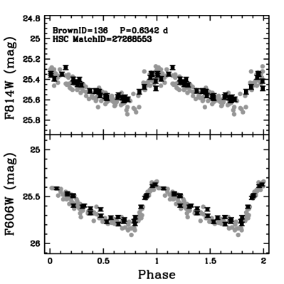
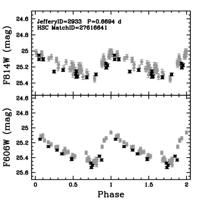
Figure 8: Light curves of two RR Lyrae stars from HSCv1 (black) and literature (grey) from Halo11 (upper panel) and the Stream (lower panel). Both are folded with the period provided in the literature.

Table 3: Published variables in the three M 31 HST fields.

Field	Published	Reference	Listed in	Recovered
	variables		HSCv1	variables
Halo11	115	Brown et al. (2004)	88	78 (89%)
Disk	21	Jeffery et al. (2011)	21	21 (100%)
Stream	24	Jeffery et al. (2011)	22	21 (95%)
All	160	Brown et al. (2004)	131	120 (92%)
		Jeffery et al. (2011)

Halo11 field

In the Halo11 field, 53 out of 55 published RR Lyrae variables have a confirmed counterpart in the HSCv1. One RR Lyrae star (V167) has not been included as it had fewer than 6 data points in the HSCv1 F814W filter LC. RR Lyrae variable V124 did not pass the point source selection, due to blending with a nearby source.

HSCv1 counterparts were confirmed for 27 out of 32 published LPVs (all 32 with amplitudes higher than 0.1 mag in both filters). Five LPVs (V14, V18, V19, V21, V25) have no HSCv1 counterpart within 1 arcsec, possibly due to their location near the globular cluster SKHB 312 (Holland et al., 1997), where severe blending can be expected. The Brown et al. (2004) list of variables also contains two anomalous Cepheid (aCep) candidates (V60, V118), one post-AGB (V84) and two RR Lyrae star candidates (V29, V6), all successfully matched within the HSCv1. Due to the shallower magnitude limit of HSCv1, we could not identify counterparts for the fainter variables published by Brown et al. (2004). Out of 8 eclipsing binary candidates only two have been matched with HSCv1 (V64 and V173). Out of 15 dwarf Cepheids only one could be reliably identified (V48) on the basis of its coordinates and location on the CMD, although the HSCv1 LC is too noisy to compare reliably with the published one.

A total of 88 known variables in the Halo11 field (53 confirmed RR Lyrae stars and 2 candidates, 27 LPVs, 2 possible anomalous Cepheids, 1 post AGB, 2 eclipsing binary candidates and 1 possible dwarf Cepheid) have HSCv1 LCs that pass our selection criteria and are expected to be recovered by our variability detection technique. Our procedure has yielded a total of 156 candidate variables when using both filters, and 128 (167) using only F606W (F814W) data. Out of the 88 known variables in the input catalog, 78 (89%) have been recovered by the variability selection method when using both filters, 90% when using only the F606W filter and 86% when using only the F814W filter. The recovery rate is higher for the F606W data compared to the F814W data, mainly due to the 1.5 times higher amplitude of RR Lyrae variables in F606W than in F814W. The variables not recovered are faint (two eclipsing binary candidates, V64 and V173, and one dwarf Cepheid, V48) or low amplitude variables (a post-AGB star V84, an LPV V158, four low amplitude RR Lyrae variables of RRc type, V40, V76, V80 and V137, and one possible RR Lyrae variable, V29). Some of these sources are also affected by problems such as possible blending, vicinity to the edge of an image, or, to a diffraction spike of a bright neighboring source.

Disk field

Jeffery et al. (2011) searched for short period variables discovering 21 RR Lyrae stars and two Cepheids in the Disk field. No reliable counterparts were found in the HSCv1 based sample for two Jeffery et al. (2011) RRc variables with IDs 15256 (due to a nebulosity) and 21631 (blending with a brighter source). We have HSCv1 LCs for 19 known RR Lyrae variables and 2 Cepheids in the Disk field.

The selection process yielded 192 candidate variables using both filters, which include all of the 21 known variables, thus yielding a 100% recovery rate. For comparison, 266 (202) candidates were found using only the F606W (F814W) filter, with a recovery rate of 100% (90%) of known variables.

Stream field

Jeffery et al. (2011) discovered 24 RR Lyrae stars in the Stream field. One of the RR Lyrae stars (ID 409) is missing from the HSCv1 based sample as it only had 5 visits in F606W filter, probably due to its location near the edge of the frame. No reliable counterpart was found for the RR Lyrae variable ID 8544, probably due to the adverse effect of a nearby nebulosity on the source extraction procedure employed for creating the HSCv1. We hence have 22 RR Lyrae stars in the Stream field successfully matched with HSCv1.

The variability selection procedure yielded 88 candidate variables using both filters, out of which 21 are in common with the Jeffery et al. (2011) list of 22 known variables in the input catalog (95% recovery rate). For comparison, 124 (96) candidates were found using only F606W (F814W) filter, with a recovery rate of 86% (91%). The only known variable not recovered is an RRc type RR Lyrae variable (ID 9975) of low amplitude ($\simeq$ 0.2 mag in F606W and $\simeq$0.15 in F814W).

4.2 New variables

Candidates that were not matched with known variables were validated using the following procedure:

1. visual inspection of the images in both filters, in order to identify probable sources of error such as: blending; proximity to a diffraction spike of another source; cosmic rays; bad column or hot pixel; proximity to the frame edge

2. inspection of the LC for the presence of outliers or inconsistencies in the appearance of variability in the two filters.

3. lack of obvious similarities with LC of other sources in the field, which may indicate systematic errors in photometry.

The source position on the CMD was used to confirm the variability type inferred from the LC, but it was not considered as a criterion when deciding whether a given source is variable or not. With the exception of a single source, 22221197, all new candidate variables that passed our visual inspection, were found to lie in either the RR-Lyrae or the LPV region of the CMD.

Table 4 summarizes the variability search results listing the field name, the total number of HSCv1 sources passing the initial quality cuts, the number of candidates obtained with the variable stars selection procedure, the number of confirmed variables together with the percentage of recovered known variables, the number of candidates that were rejected. The process of visual inspection is subjective by its nature. When presented with apparent low-amplitude variability we had to decide if a neighboring source is bright and close enough to corrupt the LC or if the LC is sufficiently different form some other LCs in the field. For about a half of the rejected candidates listed in Table 4 we had to make these judgment calls while the other half did not pass the saturation-magnitude cuts or had severe imaging problems.

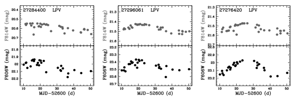
Figure 9: Sample LCs of the new variables in the Halo11 field. All LC plots are available in Appendix A.

The list of newly identified variables is presented in Table 5. For each variable the table lists the HSCv1 ID, Field, equatorial coordinates, F814W average magnitudes, number of visits in F814W, F606W average magnitudes, number of visits in F606W, classification and comments. The LCs of the new variables are presented in Fig. 9. Fig. 5, 6 and 7, which show the candidates and the confirmed new variables on the CMD together with all sources.

Table 4: Summary of confirmed and rejected candidate variables.

Field	HSCv1	Candidate	Confirmed	Rejected
	sources	variables	candidates	candidates
Halo11	7109	156	87 (89%, 9 new)	69
Disk	6732	192	41 (100%, 20 new)	151
Stream	4311	88	30 (95%, 9 new)	58
All	18152	436	158 (92%, 38 new)	278

Halo11 field

A total of 78 candidate new variables have been identified. Out of these, 13 are rejected because they are brighter than 21.0 mag in F606W and/or 20.5 mag in F814W. We visually inspected the images, LC and CMD location of 65 candidates: 30 of these are false detections: 13 (5 of which are close to globular cluster SKHB 312) are affected by blending; 15 are close to the frame edge; 1 is close to diffraction spikes of a nearby bright star; 1 is surrounded by a halo in some images. We were able to confirm 7 new variables, all LPVs. The results of visual inspection for the remaining candidates were inconclusive, so they were not included in the list of confirmed variables. The same procedure was followed for the candidates yielded by the selection procedure from the single-filter data resulting in two more confirmed LPVs.

Disk field

A total of 171 candidate new variables were identified using the two filters. Out of these, 15 are rejected as being possibly saturated. We visually inspected the remaining 156 candidates: 62 are affected by image problems of several types: 15 are blended with nearby sources, 31 are close to the frame edge, 10 are close to a nebulosity or surrounded by a halo in some images, 3 are very close diffraction spikes of nearby sources, 3 are close to hot pixels. We were able to confirm 20 new variables: 19 LPVs (one of which at the faint limit, see Table 5) and one with uncertain variability type. Visual inspection did not result in a firm classification for 74 sources.

Stream field

A total of 67 new candidate variables have been identified using both filters. Out of these, 11 have been rejected as possibly saturated. We hence visually inspected 56 candidates: 11 are affected by image problems such as 2 blended, 6 lying on the edge/very close to the edge, 2 very close diffraction spikes of nearby sources, 1 close to hot pixels. We were able to confirm 9 new variables, all LPVs (see Table 5). No other variables could be confirmed after inspecting candidates selected from the single-filter analysis.

The Stream field observations present a 20 day gap that complicates the analysis and classification of the LCs. In this case, we relied mostly on the shape of the LC in the first part of the time series. In some dubious cases (e.g. 27664093, see Figure 19), we visually inspected the LCs for the nearby sources to rule out photometric problems.

Table 5: Characteristics of new variable stars ordered by F814W average magnitudes in each field.

MatchID	Field	RA (deg)	Dec (deg)	F814W	# Visits	F606W	# Visits	Type	Comments
HSCv1		J2000	J2000	(mag)	F814W	(mag)	F606W
27284400	Halo11	11.550205	40.692210	20.586	32	22.026	27	LPV	—
27296061	Halo11	11.517188	40.681656	21.465	33	23.454	27	LPV	—
27276420	Halo11	11.518473	40.714756	21.528	33	23.064	27	LPV	—
27285008	Halo11	11.553176	40.694355	21.587	31	23.353	27	LPV	—
27273342	Halo11	11.546703	40.740814	21.635	31	23.506	27	LPV	—
27272426	Halo11	11.552447	40.733310	21.671	33	23.316	27	LPV	—
27307954	Halo11	11.502041	40.674786	21.834	17	23.806	13	LPV	F606W only
27283624	Halo11	11.523391	40.699898	21.932	32	23.184	27	LPV	F606W only
27289942	Halo11	11.504722	40.696518	22.117	33	24.310	27	LPV	—
22196858	Disk	12.289636	42.773460	20.882	16	23.270	11	LPV	—
22197833	Disk	12.296558	42.763630	21.333	16	24.384	11	LPV	—
22211719	Disk	12.291348	42.761390	21.363	16	22.572	11	LPV	—
22206385	Disk	12.283233	42.737830	21.379	16	22.310	11	LPV	—
22208821	Disk	12.296735	42.758934	21.468	16	23.315	11	LPV	—
22209236	Disk	12.301403	42.769558	21.487	16	23.414	11	LPV	—
22211391	Disk	12.315888	42.740982	21.618	16	23.468	11	LPV	—
22210819	Disk	12.296622	42.762190	21.673	16	23.573	11	LPV	—
22209784	Disk	12.253314	42.765840	21.718	16	24.904	11	LPV	—
22206501	Disk	12.294667	42.731520	21.760	12	25.256	11	LPV	—
22217682	Disk	12.296862	42.739853	21.800	16	23.691	11	LPV	—
22203253	Disk	12.269516	42.742680	21.816	16	23.324	11	LPV	—
22212431	Disk	12.262894	42.727220	21.826	16	23.603	11	LPV	—
22219207	Disk	12.290964	42.732960	21.832	16	23.294	11	LPV	—
22210620	Disk	12.250249	42.762253	21.845	16	23.980	11	LPV	—
22204580	Disk	12.321586	42.736850	21.890	16	24.706	11	LPV	—
22200824	Disk	12.298845	42.753952	21.922	16	24.031	11	LPV	—
22208319	Disk	12.278159	42.764660	22.163	12	25.869	8	LPV	—
22259268	Disk	12.277175	42.731316	22.977	16	26.348	10	LPV	faint limit in F606W
22221197	Disk	12.268279	42.742805	25.637	16	26.134	11	other	—
27663814	Stream	11.041388	39.788070	21.490	15	23.836	10	LPV	—
27661867	Stream	11.066272	39.778630	21.498	15	24.351	10	LPV	—
27654057	Stream	11.091002	39.781937	21.624	15	23.641	10	LPV	—
27659783	Stream	11.071672	39.786972	21.704	15	24.404	9	LPV	—
27664545	Stream	11.090615	39.765050	21.979	15	23.580	10	LPV	—
27665958	Stream	11.089661	39.768350	21.980	15	24.179	10	LPV	—
27664093	Stream	11.099528	39.772636	22.296	15	24.089	10	LPV	—
27630664	Stream	11.091218	39.797176	22.421	15	23.014	10	LPV	—
27619606	Stream	11.088532	39.802055	22.441	15	24.915	10	LPV	—

5 Discussion

The application of PCA to variability indices that characterize LCs allowed us to statistically select candidate variable sources using the admixture coefficients of the first two PCs, $a_{1}$ and $a_{2}$. The recovery rate of known variables in the fields studied has been more than $\simeq$90% in all cases, while 38 new variables were identified. We also confirmed that various issues that can affect the photometry, such as saturated pixels, blending, proximity to diffraction spikes, cosmic rays etc., significantly increase the number of false positives, thus making visual inspection of the automatically selected candidates imperative.

The need for visual inspection of candidate variables is common for all types of variability search (e.g. Bernard et al., 2010; Cusano et al., 2013; Abbas et al., 2014; Ramsay et al., 2014; Klagyivik et al., 2016; Pawlak et al., 2016). The underlying problem is that corrupted measurements cannot be reliably identified in all cases. Individual outlier measurements in a LC can be removed by sigma-clipping (e.g. Kim & Bailer-Jones, 2016) or tolerated thanks to the use of robust variability features (Pérez-Ortiz et al., 2017). However, these measures will not solve the problem if a given object has a large fraction of its measurements corrupted. Despite the progress in automatic rejection of imaging artifacts (Fruchter & Hook, 2002; Desai et al., 2016), visual inspection of images (Melchior et al., 2016) and LCs remains a valuable quality control tool. The goal of an automated variability detection algorithm is to minimize the percentage of false candidates passed to the visual inspection stage (Fruth et al., 2012). The PCA-based variability search is doing well in this regard when compared to other variability detection techniques applied to the same LC data (Sec. 5.4).

5.1 Physical Interpretation of the Principal Components

Each PC is a linear combination of all the input variability indices listed in Table 2:

$$\mathbf{PC_{i}}=c_{i,1}\chi_{\rm red}^{2}\mathbf{l_{1}}+c_{i,2}\sigma\mathbf{l_{2}}+c_{i,3}{\rm MAD}\mathbf{l_{3}}+c_{i,4}{\rm IQR}\mathbf{l_{4}}+\dots$$ (2)

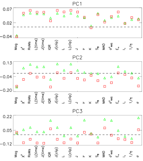
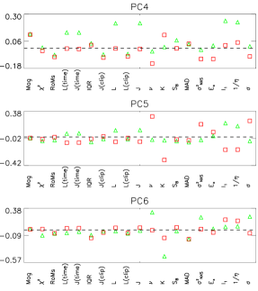
Figure 12: The first six principal components for the M 31 Disk data set. The dashed line indicates zero contribution of an index to the PC. Green triangles correspond to F606W, red squares to F814W.

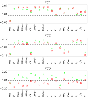
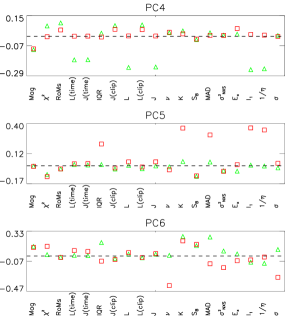
Figure 13: Same as Fig. 12 but for the Stream field.

where $c_{i,1}$, $c_{i,2}$, $c_{i,3}$, $c_{i,4}\dots$ are the coefficients determining the contribution of each index to the $i$th principal component, $\mathbf{PC_{i}}$; $\mathbf{l_{1}}$, $\mathbf{l_{2}}$, $\mathbf{l_{3}}$, $\mathbf{l_{4}}\dots$ are the unit vectors setting the directions of the $\chi_{\rm red}^{2}$, $\sigma$, ${\rm MAD}$, ${\rm IQR}\dots$ axes in the variability index space. As there are different ranges for the numerical values of the variability indices, they are standardized (as described in Sec. 3.3) before entering the equation (2). Figure 10 presents the contributions, $c_{i,j}$, of the variability indices to the first six principal components for the M 31 Halo11 PCA results. The dashed line indicates zero contribution of an index to the PC (the values of indices near that line have no effect on the PC value). The larger the distance of an index from the zero contribution line, the more it contributes to this PC. A qualitatively similar relative contribution of the variability indexes to the first few PCs is found in the Disk and Stream fields (Figures 12, 13).

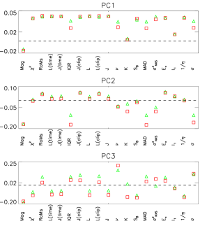
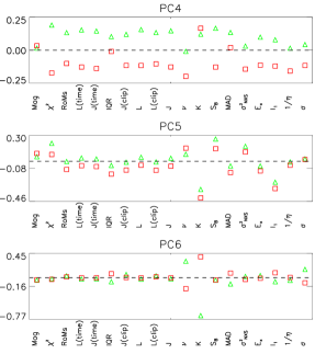
Figure 10: Coefficients $c_{i,j}$ determining relative contributions of variability indices to the first six principal components for the M 31 Halo11 data set; see equation (2). The indices computed using the F606W LCs are shown with green triangles and the ones computed using the F814W LCs are shown as red squares. The dashed line indicates zero contribution of an index to the PC.

Most variability indices contribute significantly to $\mathbf{PC_{1}}$. This is expected, since by construction the indices highlight variability. $\mathbf{PC_{1}}$ is dominated by three scatter-based indices that take into account the estimated photometric errors ($\chi^{2}$, RoMS, $\sigma^{2}_{NXS}$; see Table 2) and several correlation-based indices (L, J, S_B, E_X, $1/\eta$). The remaining scatter-based indices (IQR, MAD, $\sigma$; the first two being robust measures of scatter not relying on photometric errorbars) contribute to $\mathbf{PC_{1}}$ as well, but they are the main contributors to $\mathbf{PC_{2}}$ together with the magnitude. The admixture coefficient of $\mathbf{PC_{1}}$, $a_{1}$, has a large positive value for a bright source showing smooth high-amplitude lightcurve. The value of $a_{2}$ is large and negative for a faint source with a lightcurve that is not smooth and is showing a large scatter that is not driven by a few outlier points. $\mathbf{PC_{3}}$–$\mathbf{PC_{6}}$ show no easily interpretable patterns, while together they account for 15% of the total data variance. These components are expected to represent rare information encoded into the variability indices. $K$ and $l_{1}$ that do not contribute to $\mathbf{PC_{1}}$ and $\mathbf{PC_{2}}$ show more significant contribution to the higher order PCs and in particular $\mathbf{PC_{5}}$. As discussed in Section 5.4 (Table 6), the $K$ index (being a robust measure of kurtosis of the distribution of magnitudes in a lightcurve) cannot identify known variables when used on its own ($F_{1}=0$; c.f. Friedrich, Koenig, & Wicenec, 1997). It does not contribute to $\mathbf{PC_{1}}$ and contributes little to $\mathbf{PC_{2}}$ (Fig. 10).

It is interesting to note that although in $\mathbf{PC_{1}}$ and $\mathbf{PC_{2}}$ the variability indices computed in the two filters show similar behavior, this is not the case for the higher order PCs. Therefore, the higher order PCs highlight differences between LCs in two filters (color changes).

As the $\mathbf{PC_{2}}$ is dominated by the indices that are robust measures of scatter while the correlation-based indices contribute less to the $\mathbf{PC_{2}}$, it becomes possible to separate short and long period variables on the $a_{1}$–$a_{2}$ admixture coefficient plots. RR Lyrae variables (marked with blue circles in Fig. 4) have short periods and uncorrelated LCs, for the cadence of the available observations, thus yielding low absolute values for $a_{1}$ and higher values for $a_{2}$. On the contrary, LPVs (marked with red squares in Fig. 4) show smooth LCs with a high degree of correlation between measurements taken close in time and hence higher values of $a_{1}$. As it can be clearly seen in the left panel of Figure 4 the two types of variables are clearly separated in the $a_{1}$–$a_{2}$ plane. The two first PCs are effective not only in separating variable from constant sources, but also in distinguishing RR Lyrae variables from LPVs, without the need of constructing a CMD. In general, “fast” and “slow” (compared to the observing cadence) variables occupy separate locations in the $a_{1}$–$a_{2}$ plane. There are only few variables of types other than RR Lyrae and LPV in the studied fields to check if further type separation is possible using admixture coefficients of higher-order PCs.

Many candidate variable sources that were not confirmed by our visual inspection of LCs and images occupy a distinct region on the $a_{1}$–$a_{2}$ plane (for the Halo 11 field $a_{1}\leq 100$ and $a_{2}\geq 12$, cf. Figure  4). The Disk and Stream fields show a similar location of RR Lyrae stars, LPVs and (some) false candidates in the admixture coefficient space (see Appendix).

5.2 Selection efficiency on the $a_{1}$–$a_{2}$ plane

As described in Section 3.4, the selection process was performed in two steps. Examination of the resulting candidates from the first selection step alone, indicated a recovery level of known variables of $\simeq 80$%, which is significantly lower than the recovery level achieved when using the fine-tuning process ($\simeq 90$%, for the Halo11 field as an example). On the other hand, the initial selection yields about half the artifacts selected with fine-tuning. The artifacts that are not included in the initial selection are mostly caused by image problems, while the majority of the artifacts common in both selections are bright sources (probably affected by saturated pixels). All new variables were selected as such in both steps. Therefore, selection of variables using only the first step described in Section 3.4, provides lower completeness (as indicated by the lower recovery rate of known variables) but higher purity (i.e. lower incidence of artifacts). Application of the fine-tuning step, provides higher completeness, but lower purity (thus increasing the number of sources that need to be expert validated). If the number of input lightcurves is very large, one may prefer to use only the first candidate selection step to reduce the number of candidates that has to be expected (increase the purity of the candidate list at the cost of its completeness).

5.3 Reduced number of source and visits

The PCA-based variability detection method proposed here is a statistical method, that requires a substantial sample of sources (variable and constant) in order to identify candidate variables. Here we investigate the applicability of the method, when the size of the sample is reduced significantly. We divided the Halo11 sample into subsamples of different sizes, ranging from 6500 to 500 sources, in steps of 500. We then applied the PCA variability detection method for each subsample and calculated the recovery rate of known variables from Brown et al. (2004) that happen to be included in the specific subsample. The tests were repeated 100 times for each subsample size, each time randomly selecting the specified number of sources from the full sample. The average recovery rate was not affected significantly. This test indicates that the method can be applied even to relatively small samples with as few as 500 sources.

An additional sensitivity test was performed to evaluate the efficiency of our method when the number of data points in the LC is reduced. The experiment was conducted using the Halo11 LCs. Epochs were randomly omitted from the LCs and the PCA and selection analysis repeated each time, following the same steps as described in Section 3. The experiment was repeated for 30, 20, 10 and 5 data points in the LC. We do not consider LCs with smaller number of points, as the variability indices (Table 2), while being mathematically defined, are expected to lose their predictive power.

The decrease of the number of points in the LC expectedly increases the size of the constant star locus on the $a_{1}$–$a_{2}$ plane, thus degrading the detectability of variables that lie close to the constant star locus in the original selection plane of Figure 4 (upper left panel). When only 5 points are retained in the LC, additional 10 known variables are not recovered, reducing the recovery rate to $\simeq$77%, without appreciably increasing the false variable detection. This is still an acceptable result, indicating that the method can be successful even with a small number of epochs in the LC.

5.4 Comparison with a single-index search

We compare our new variability detection technique relying on identification of isolated points in the ($a_{1}$, $a_{2}$) plane (presented in Section 3) to the conventional methods discussed by Sokolovsky et al. (2017a). These methods identify candidate variables as objects having a value of a single variability index (Table 2) above some magnitude-dependent threshold (Fig. 11). The indices are computed independently for F606W and F814W LCs. The authors also suggested to use $a_{1}$ as a composite variability index. We test this approach (Fig. 11, top panel) combining in $a_{1}$ for each object all the variability indexes computed using its LCs in F606W and F814W bands.

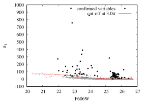
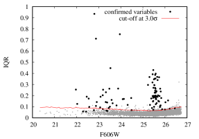
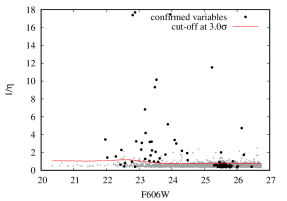
Figure 11: Candidate variable selection in the Halo11 field above magnitude-dependents cuts (solid line) in $a_{1}$, ${\rm IQR}$ and $1/\eta$ (Table 2).

To evaluate the quality of a variability search in a given set of LCs we need to know the ground truth: which objects are variable and which are not. As a working approximation of this we use a list of variables found by Brown et al. (2004) and Jeffery et al. (2011) cross-matched with the HSC (Table 3) together with the results of our visual inspection of candidate variables identified with the ($a_{1}$, $a_{2}$) technique (Sec. 4.2). Following Sokolovsky et al. (2017a); Pashchenko, Sokolovsky, & Gavras. (2017) we adopt the $F_{1}$-score (van Rijsbergen, 1974) as the success metric of variability detection. The $F_{1}$-score

$$F_{1}=2(C\times P)/(C+P)$$ (3)

is defined through the completeness $C$ (also known as “recall”) and purity $P$ (“precision”) of the list of candidate variables (Graham et al., 2014):

$$C=\frac{\mathrm{Number\,\,of\,\,variables\,\,in\,\,the\,\,list}}{\mathrm{Total\,\,number\,\,of\,\,variables\,\,in\,\,the\,\,field}}$$ (4)

$$P=\frac{\mathrm{Number\,\,of\,\,variables\,\,in\,\,the\,\,list}}{\mathrm{Total\,\,number\,\,of\,\,candidates\,\,in\,\,the\,\,list}}.$$ (5)

$F_{1}=1$ for the perfect selection of variables when one retrieves all the true variables and no false candidates while $F_{1}=0$ if no true variables got into the list of candidates.

Table 6: Variability detection efficiency ($F_{1}$-score).

Index	Filter	Halo11	Disk	Stream
PCA-based search
($a_{1}$, $a_{2}$)		0.628	0.434	0.595
$a_{1}$		0.564	0.373	0.530
Scatter-based indices
$\chi_{\rm red}^{2}$	F606W	0.419	0.154	0.260
$\chi_{\rm red}^{2}$	F814W	0.344	0.151	0.316
$\sigma$	F606W	0.532	0.230	0.412
$\sigma$	F814W	0.402	0.180	0.440
${\rm MAD}$	F606W	0.657	0.308	0.442
${\rm MAD}$	F814W	0.467	0.281	0.633
${\rm IQR}$	F606W	0.617	0.347	0.488
${\rm IQR}$	F814W	0.516	0.380	0.593
${\rm RoMS}$	F606W	0.602	0.304	0.454
${\rm RoMS}$	F814W	0.528	0.322	0.547
$\sigma_{\rm NXS}^{2}$	F606W	0.381	0.137	0.258
$\sigma_{\rm NXS}^{2}$	F814W	0.314	0.126	0.290
$v$	F606W	0.447	0.195	0.371
$v$	F814W	0.350	0.146	0.323
$K$	F606W	0.000	0.000	0.000
$K$	F814W	0.000	0.000	0.000
Correlation-based indices
$J$	F606W	0.551	0.429	0.447
$J$	F814W	0.396	0.354	0.444
$J({\rm time})$	F606W	0.494	0.361	0.467
$J({\rm time})$	F814W	0.373	0.295	0.410
$J({\rm clip})$	F606W	0.671	0.381	0.542
$J({\rm clip})$	F814W	0.566	0.335	0.552
$L$	F606W	0.553	0.359	0.379
$L$	F814W	0.404	0.336	0.354
$L({\rm time})$	F606W	0.481	0.372	0.467
$L({\rm time})$	F814W	0.391	0.298	0.378
$L({\rm clip})$	F606W	0.660	0.376	0.504
$L({\rm clip})$	F814W	0.557	0.379	0.567
$E_{x}$	F606W	0.505	0.158	0.246
$E_{x}$	F814W	0.379	0.193	0.232
$l_{1}$	F606W	0.271	0.107	0.000
$l_{1}$	F814W	0.068	0.037	0.000
$1/\eta$	F606W	0.193	0.099	0.055
$1/\eta$	F814W	0.176	0.091	0.056
$S_{B}$	F606W	0.257	0.099	0.146
$S_{B}$	F814W	0.232	0.104	0.121

The $F_{1}$-score is defined by equation (3); see Table 2 for additional information on the variability indices.

Table 6 compares the $F_{1}$-scores reached by the PCA-based and the conventional single-index techniques in the three investigated fields. For each individual index we use a $3\sigma$ threshold to select candidate variables. Despite a smaller median number of visits (Table 1), for most individual variability indices the F606W LCs result in higher $F_{1}$-scores than the F814W LCs. This may be attributed to the fact that pulsating stars tend to have higher variability amplitudes at shorter wavelengths and are therefore easier to distinguish from non-variable stars.

The PCA-based search results in consistently high $F_{1}$ values compared to candidate selection based on most individual indices, however the PCA $F_{1}$ is the highest one only in the Disk field. In the Halo11 field, the PCA search is outperformed by ${\rm MAD}$, $J({\rm clip})$ and $L({\rm clip})$ computed on F606W LCs. In the Stream field ${\rm MAD}$ computed on the F814W LCs results in the $F_{1}$ value higher than the one we obtain with the PCA, while ${\rm IQR}$ (F814W) results in only a slightly lower $F_{1}$. The ${\rm MAD}$ computed for F606W LCs results in much lower $F_{1}$ values compared to ${\rm MAD}$–F814W in the Stream field, while in the Halo 11 field it is the opposite: ${\rm MAD}$–F606W has the $F_{1}$-score much higher than ${\rm MAD}$–F814W. Our PCA variability search based on two admixture coefficients ($a_{1}$, $a_{2}$) for all three fields results in higher $F_{1}$ values compared to the PCA-based approach relying on a magnitude dependent cut in $a_{1}$ considered by Sokolovsky et al. (2017a).

It is hard to predict which index will be the most efficient variability indicator in a given data set. The efficiency of an index in identifying variables depends on variability type, observing cadence, percentage of outlier measurements and the level of correlated (systematic) noise in the data. The authors suggested ${\rm IQR}$ and $1/\eta$ as the indices that tend to perform well on diverse test data, while not necessarily being the best indices for any given data set. In the Halo11, Disk and Stream data sets considered here, ${\rm IQR}$ is among the best variability indices, while $1/\eta$ is among the worst ones. This is easily understood as $1/\eta$ being the measure of correlation (smoothness) of a lightcurve is unable to detect the numerous RR Lyrae variables in these data sets. The observing cadence is long compared to RR Lyrae periods, making their LCs appear smooth only when folded with the correct period (Fig. 8). Only the LPVs which have smooth LCs plotted as as a function of time can be identified with $1/\eta$ (and other correlation-based indices).

The PCA-based search results in higher $F_{1}$ values compared to both ${\rm IQR}$ and $1/\eta$ for the three studied fields. ${\rm MAD}$, another outlier resistant index, may show both higher and lower $F_{1}$-scores compared to both ${\rm IQR}$ and the PCA-based search, depending of field and filter. This suggests that, unless it is somehow known a priory which variability index is the best one for the studied data set, it is more efficient (in terms of archiving a higher $F_{1}$-score) to compute multiple variability indices and combine them via the PCA rather than use the “safe” indices, ${\rm MAD}$, ${\rm IQR}$ and $1/\eta$.

While the PCA constructs a linear combination of indices, machine-learning may help to find useful non-linear combinations of indices resulting in higher $F_{1}$-scores (Pashchenko, Sokolovsky, & Gavras., 2017). However, a variability search based on supervised machine learning requires a representative training set of LCs pre-classified as variable or non-variable by some other means and thus cannot be used for a blind variability search in a small field. Training a machine learning classifier on LCs obtained with one survey and then applying this classifier to LCs from another survey (“knowledge transfer”), while being in principle possible, remains an unsolved problem in practice. Variability search based on unsupervised machine learning may be a promising approach for conducting blind variability surveys (e.g. Shin et al., 2009, 2012; Mackenzie, Pichara, & Protopapas, 2016).

6 Conclusions

We investigate a new method of variable object detection in a large set of light curves, which is based on principal component analysis. Each light curve is characterized by its mean magnitude and a set of variability indices (Table 2) that are used as the input for the PCA. Candidate variable objects are identified as outliers in the plane of admixture coefficients $a_{1}$–$a_{2}$ corresponding to the two most significant principal components. The proposed method is suitable for (and most efficient in) large sets of LCs. It requires no a priori information about the type of the searched variable objects. Instead it relies on assumptions that variable objects are rare and the indices listed in Table 2 are able to capture variability information – the assumptions that hold true for most ground-based and many space-based observations in optical and near-infrared bands. This methodology can indeed successfully identify variable stars not only in the HSC database, but also in ground based data with different sample sizes and epochs as discussed in Section 5.3. There is no need to preselect the “best” variability indices for different samples, since PCA outputs their optimal linear combinations. Human intervention is still necessary to validate the resulting candidate variables (see discussion in 5.2). The present algorithm is performed in the framework of the HCV, which will be available in 2018.

The method is verified using 18152 LCs of stars in 3 fields in M 31 extracted from the Hubble Source Catalogue. We recovered about 90% of the known variables reported by Brown et al. (2004) and Jeffery et al. (2011). We found 38 new variable stars, among which 37 LPVs and one object of an uncertain variability type (Table 5). This demonstrates that the Hubble Source Catalogue, despite its shallower depth and reduced time resolution compared to what can be obtained with dedicated manual analysis of the archival HST images, includes many previously unknown variable objects in fields previously studied for variability.

Appendix A Disk and Stream Fields

In this appendix we show similar figures as those included in the main part of the paper but for the Disk and Stream fields. The presentation and discussion provided for field Halo11 are also applicable to the Disk and Stream fields unless specifically indicated. We also present the LCs of all new variables identified in the Halo11 (Fig. 16), Disk (Fig. 17) and Stream (Fig. 19) fields.

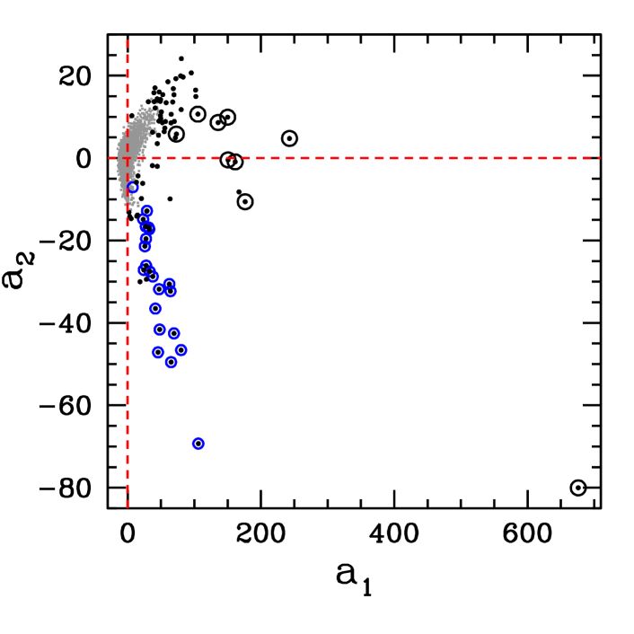
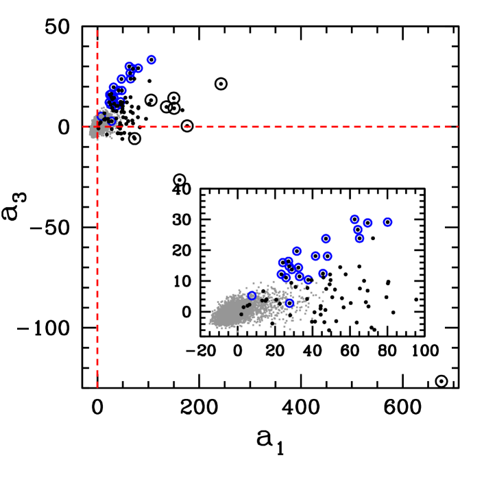
Figure 15: Same as Figure 4, but for the M 31 Stream. The candidate variables obtained with the method described in Section 3.4 are highlighted with black points, while newly discovered variables are marked with big black open circles. Small blue open circles highlight RR Lyrae variables from Jeffery et al. (2011).

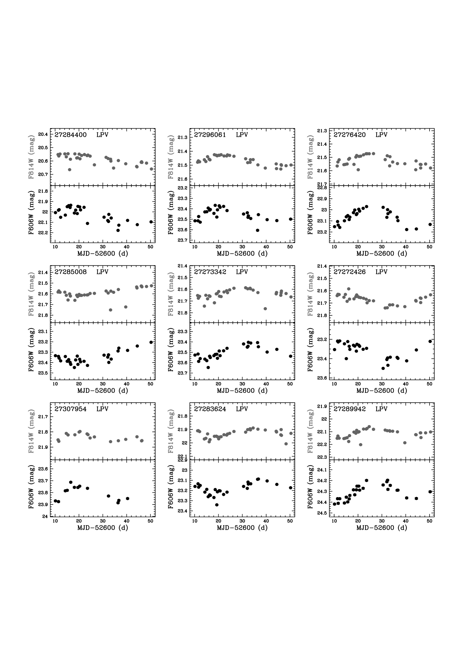
Figure 16: Light curves for the new variables in the Halo11 field, ordered by F814W magnitude.

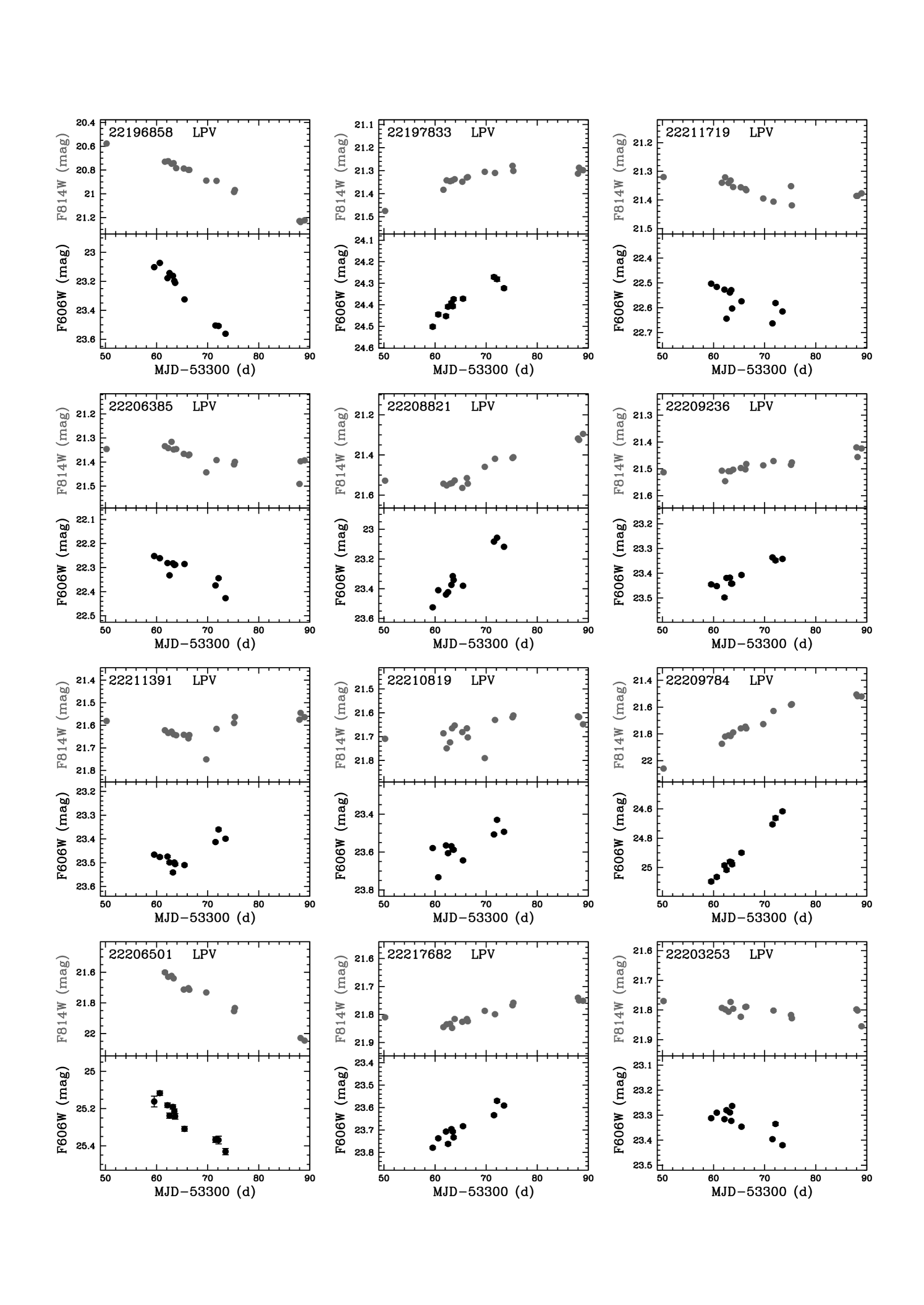
Figure 17: Light curves for the new variables in the Disk field, ordered by F814W magnitude.

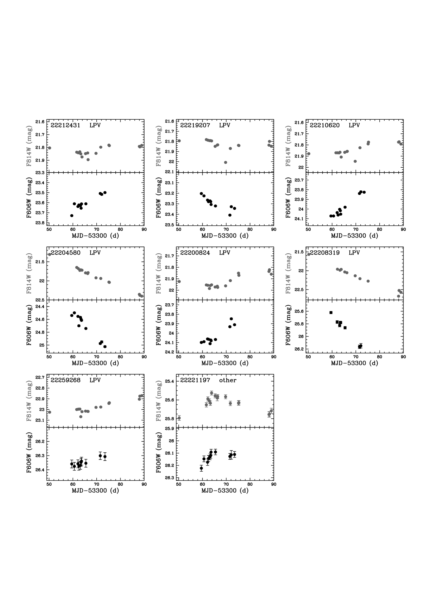
Figure 18: continued

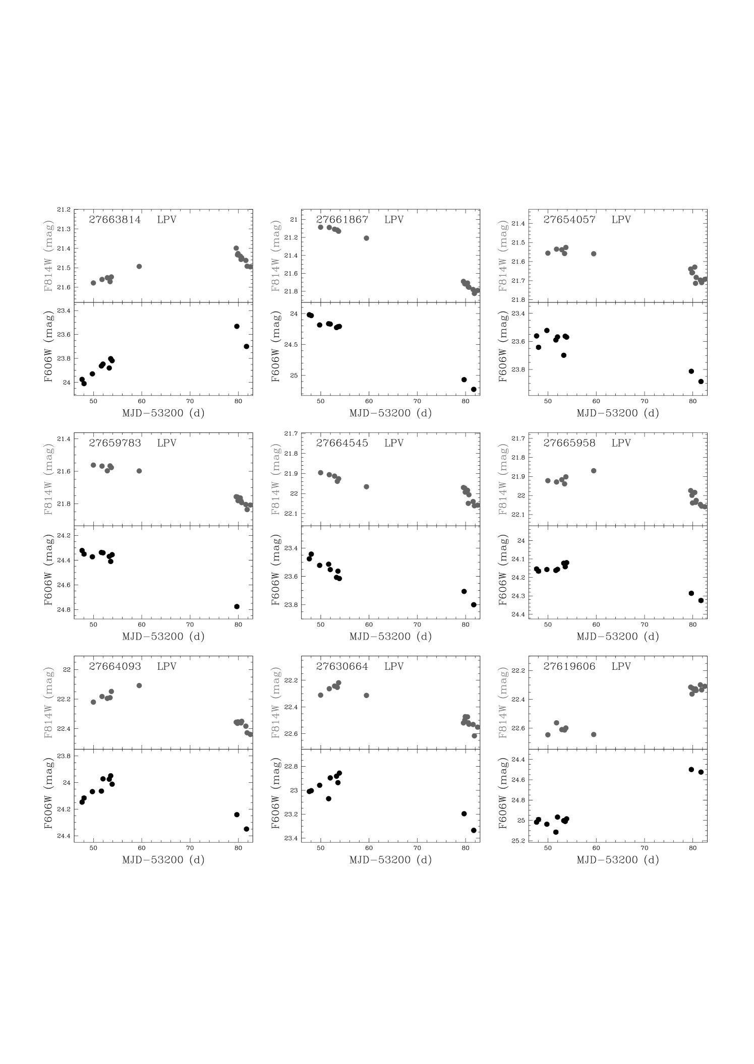
Figure 19: Light curves for the new variables in the Stream field, ordered by F814W magnitude.

References

- Abbas et al. (2014) Abbas M. A., Grebel E. K., Martin N. F., Burgett W. S., Flewelling H., Wainscoat R. J., 2014, MNRAS, 441, 1230
- Ahn et al. (2014) Ahn C. P., et al., 2014, ApJS, 211, 17
- Alonso et al. (2007) Alonso, R., Brown, T. M., Charbonneau, D., et al. 2007, Transiting Extrasolar Planets Workshop, 366, 13
- Angeloni et al. (2014) Angeloni R., et al., 2014, A&A, 567, A100
- Auvergne et al. (2009) Auvergne, M., Bodin, P., Boisnard, L., et al. 2009, A&A , 506, 411
- Bailer-Jones et al. (1998) Bailer-Jones, C. A. L., Irwin, M., & von Hippel, T. 1998, MNRAS , 298, 361
- Bakos et al. (2004) Bakos, G., Noyes, R. W., Kovács, G., et al. 2004, PASP , 116, 266
- Benedict et al. (2017) Benedict G. F., McArthur B. E., Nelan E. P., Harrison T. E., 2017, PASP, 129, 012001
- Bernard et al. (2010) Bernard E. J., et al., 2010, ApJ, 712, 1259
- Bernard et al. (2013) Bernard E. J., et al., 2013, MNRAS, 432, 3047
- Bertin & Arnouts (1996) Bertin, E., & Arnouts, S. 1996, A&A Supp. , 117, 393
- Bonanos & Stanek (2003) Bonanos, A. Z., & Stanek, K. Z. 2003, ApJL , 591, L111
- Borucki et al. (2010) Borucki, W. J., Koch, D., Basri, G., et al. 2010, Science, 327, 977
- Brown et al. (1989) Brown, L. M. J., Robson, E. I., Gear, W. K., & Smith, M. G. 1989, ApJ , 340, 150
- Brown et al. (2003) Brown, T. M., Ferguson, H. C., Smith, E., et al. 2003, ApJL , 592, L17
- Brown et al. (2004) Brown, T. M., Ferguson, H. C., Smith, E., et al. 2004, AJ , 127, 2738
- Brown et al. (2006) Brown, T. M., Smith, E., Ferguson, H. C., et al. 2006, ApJ , 652, 323
- Brown et al. (2009) Brown, T. M., Smith, E., Ferguson, H. C., et al. 2009, Astrop. J. Supp. , 184, 152
- Budavári & Lubow (2012) Budavári, T., & Lubow, S. H. 2012, ApJ , 761, 188
- Burdanov et al. (2016) Burdanov A. Y., et al., 2016, MNRAS, 461, 3854
- Butters et al. (2010) Butters, O. W., West, R. G., Anderson, D. R., et al. 2010, A&A , 520, L10
- Chambers et al. (2016) Chambers K. C., et al., 2016, arXiv:1612.05560
- Chazelas et al. (2012) Chazelas B., et al., 2012, SPIE, 8444, 84440E
- Christ, Kempa-Liehr, & Feindt (2016) Christ M., Kempa-Liehr A. W., Feindt M., 2016, arXiv:1610.07717
- Cioni et al. (2011) Cioni M.-R. L., Clementini G., Girardi L., et al. 2011, A&A , 527, A116
- Clementini et al. (2009) Clementini, G., Contreras, R., Federici, L., et al. 2009, ApJL , 704, L103
- Clementini et al. (2016) Clementini, G., Ripepi, V., Leccia, S., et al. 2016, A&A , 595, A133
- Cusano et al. (2013) Cusano F., et al., 2013, ApJ, 779, 7
- Debosscher et al. (2007) Debosscher, J., Sarro, L. M., Aerts, C., et al. 2007, A&A , 475, 1159
- Debosscher et al. (2009) Debosscher, J., Sarro, L. M., López, M., et al. 2009, A&A , 506, 519
- de Diego (2010) de Diego, J. A. 2010, AJ , 139, 1269
- Desai et al. (2016) Desai S., Mohr J. J., Bertin E., Kümmel M., Wetzstein M., 2016, A&C, 16, 67
- de Souza et al. (2014) de Souza, R. S., Maio, U., Biffi, V., & Ciardi, B. 2014, MNRAS , 440, 240
- Di Criscienzo et al. (2011) Di Criscienzo, M., Greco, C., Ripepi, V., et al. 2011, AJ , 141, 81
- Drake et al. (2009) Drake, A. J., Djorgovski, S. G., Mahabal, A., et al. 2009, ApJ , 696, 870
- Drake et al. (2014) Drake A. J., et al., 2014, ApJS, 213, 9
- Dutta et al. (2018) Dutta S., Mondal S., Joshi S., Jose J., Das R., Ghosh S., 2018, arXiv:1802.02303
- Eyer (2006) Eyer, L. 2006, Astrophysics of Variable Stars, 349, 15
- Ferreira Lopes & Cross (2016a) Ferreira Lopes, C. E., & Cross, N. J. G. 2016, A&A , 586, A36
- Ferreira Lopes & Cross (2017) Ferreira Lopes, C. E., & Cross, N. J. G. 2017, A&A , 604, A121
- Figuera Jaimes et al. (2013) Figuera Jaimes, R., Arellano Ferro, A., Bramich, D. M., Giridhar, S., & Kuppuswamy, K. 2013, A&A , 556, A20
- Fiorentino et al. (2013) Fiorentino, G., Musella, I., & Marconi, M. 2013, MNRAS , 434, 2866
- Fiorentino et al. (2010) Fiorentino, G., Contreras Ramos, R., Clementini, G., et al. 2010, ApJ , 711, 808
- Freedman et al. (2001) Freedman, W. L., Madore, B. F., Gibson, B. K., et al. 2001, ApJ , 553, 47
- Friedrich, Koenig, & Wicenec (1997) Friedrich S., Koenig M., Wicenec A., 1997, ESASP, 402, 441
- Fruchter & Hook (2002) Fruchter A. S., Hook R. N., 2002, PASP, 114, 144
- Fruth et al. (2012) Fruth, T., Kabath, P., Cabrera, J., et al. 2012, AJ , 143, 140
- Gaia Collaboration et al. (2016) Gaia Collaboration, Prusti, T., de Bruijne, J. H. J., et al. 2016, A&A , 595, A1
- Gavras et al. (2017) Gavras, P., Bonanos, A. Z., Bellas-Velidis, I., et al. 2017, IAU Symposium, 325, 369
- Graham et al. (2014) Graham M. J., Djorgovski S. G., Drake A. J., Mahabal A. A., Chang M., Stern D., Donalek C., Glikman E., 2014, MNRAS, 439, 703
- Griest et al. (1991) Griest, K., Alcock, C., Axelrod, T. S., et al. 1991, ApJL , 372, L79
- Graham et al. (2013) Graham, M. J., Drake, A. J., Djorgovski, S. G., et al. 2013, MNRAS , 434, 3423
- Hoffmann et al. (2016) Hoffmann S. L., et al., 2016, ApJ, 830, 10
- Holland et al. (1997) Holland, S., Fahlman, G. G., & Richer, H. B. 1997, AJ , 114, 1488
- Horne & Baliunas (1986) Horne, J. H., & Baliunas, S. L. 1986, ApJ , 302, 757
- Ibata et al. (2001) Ibata, R., Irwin, M., Lewis, G., Ferguson, A. M. N., & Tanvir, N. 2001, Nature , 412, 49
- Ishida & de Souza (2013) Ishida, E. E. O., & de Souza, R. S. 2013, MNRAS , 430, 509
- Ivezic et al. (2008) Ivezic Z., et al., 2008, arXiv:0805.2366
- Jeffery et al. (2011) Jeffery, E. J., Smith, E., Brown, T. M., et al. 2011, AJ , 141, 171
- Karampelas et al. (2012) Karampelas, A., Kontizas, M., Rocca-Volmerange, B., et al. 2012, A&A , 538, A38
- Kim et al. (2011) Kim, D.-W., Protopapas, P., Alcock, C., Byun, Y.-I., & Khardon, R. 2011, Astronomical Data Analysis Software and Systems XX, 442, 447
- Kim et al. (2014) Kim, D.-W., Protopapas, P., Bailer-Jones, C. A. L., et al. 2014, A&A , 566, A43
- Kim & Bailer-Jones (2016) Kim, D.-W., & Bailer-Jones, C. A. L. 2016, A&A , 587, A18
- Kirihara et al. (2017) Kirihara, T., Miki, Y., Mori, M., Kawaguchi, T., & Rich, R. M. 2017, MNRAS , 464, 3509
- Klagyivik et al. (2016) Klagyivik P., et al., 2016, AJ, 151, 110
- Koch et al. (2010) Koch, D.G., Borucki, W.J., Basri, G. et al., 2010, ApJ , 713, 79
- Kolesnikova et al. (2008) Kolesnikova, D. M., Sat, L. A., Sokolovsky, K. V., Antipin, S. V., & Samus, N. N. 2008, Acta Astron. , 58, 279
- Kügler, Gianniotis, & Polstere (2015) Kügler S. D., Gianniotis N., Polsterer K. L., 2015, MNRAS, 451, 3385
- Laher et al. (2017) Laher R. R., et al., 2017, arXiv:1708.01584
- Law et al. (2009) Law, N. M., Kulkarni, S. R., Dekany, R. G., et al. 2009, PASP , 121, 1395
- Lasker et al. (2008) Lasker, B. M., Lattanzi, M. G., McLean, B. J., et al. 2008, AJ , 136, 735
- Layden et al. (1999) Layden A. C., Ritter L. A., Welch D. L., Webb T. M. A., 1999, AJ, 117, 1313
- Mackenzie, Pichara, & Protopapas (2016) Mackenzie C., Pichara K., Protopapas P., 2016, ApJ, 820, 138
- Medina et al. (2018) Medina G., et al., 2018, arXiv, arXiv:1802.01581
- McCommas et al. (2009) McCommas L. P., Yoachim P., Williams B. F., Dalcanton J. J., Davis M. R., Dolphin A. E., 2009, AJ, 137, 4707
- Melchior et al. (2016) Melchior P., et al., 2016, A&C, 16, 99
- Minniti et al. (2010) Minniti, D., Lucas, P. W., Emerson, J. P., et al. 2010, New Astronomy , 15, 433
- Mowlavi (2014) Mowlavi N., 2014, A&A, 568, A78
- Nandra et al. (1997) Nandra, K., George, I. M., Mushotzky, R. F., Turner, T. J., & Yaqoob, T. 1997, ApJ , 476, 70
- Nun et al. (2015) Nun, I., Protopapas, P., Sim, B., et al. 2015, arXiv:1506.00010
- Oelkers et al. (2018) Oelkers R. J., et al., 2018, AJ, 155, 39
- Paegert et al. (2014) Paegert, M., Stassun, K. G., & Burger, D. M. 2014, AJ , 148, 31
- Parks et al. (2014) Parks, J. R., Plavchan, P., White, R. J., & Gee, A. H. 2014, Astrop. J. Supp. , 211, 3
- Pashchenko, Sokolovsky, & Gavras. (2017) Pashchenko I. N., Sokolovsky K. V., Gavras P., 2017, arXiv:1710.07290
- Pawlak et al. (2016) Pawlak M., et al., 2016, AcA, 66, 421
- Pearson (1901) Pearson K., 1901, Philosophical Magazine Series 6, 2, 11, 559
- Pepper et al. (2007) Pepper, J., Pogge, R. W., DePoy, D. L., et al. 2007, PASP , 119, 923
- Pérez-Ortiz et al. (2017) Pérez-Ortiz M. F., García-Varela A., Quiroz A. J., Sabogal B. E., Hernández J., 2017, A&A, 605, A123
- Perryman et al. (2001) Perryman, M. A. C., de Boer, K. S., Gilmore, G., et al. 2001, A&A , 369, 339
- Pojmanski (2002) Pojmanski, G. 2002, Acta Astron. , 52, 397
- Re Fiorentin et al. (2007) Re Fiorentin, P., Bailer-Jones, C. A. L., Lee, Y. S., et al. 2007, A&A , 467, 1373
- Ramsay et al. (2014) Ramsay G., et al., 2014, MNRAS, 437, 132
- Richards et al. (2011) Richards, J. W., Starr, D. L., Butler, N. R., et al. 2011, ApJ , 733, 10
- Ricker et al. (2014) Ricker G. R., et al., 2014, SPIE, 9143, 914320
- Rose & Hintz (2007) Rose, M. B., & Hintz, E. G. 2007, AJ , 134, 2067
- Samus et al. (2017) Samus N. N., Kazarovets E. V., Durlevich O. V., Kireeva N. N., Pastukhova E. N., 2017, ARep, 61, 80
- Sesar et al. (2017) Sesar B., et al., 2017, AJ, 153, 204
- Shappee et al. (2014) Shappee, B.J., Prieto, J.L., Grupe, D., et al., 2014, ApJ , 788, 48
- Shin et al. (2009) Shin, M.-S., Sekora, M., & Byun, Y.-I. 2009, MNRAS , 400, 1897
- Shin et al. (2012) Shin M.-S., Yi H., Kim D.-W., Chang S.-W., Byun Y.-I., 2012, AJ, 143, 65
- Skrutskie et al. (2006) Skrutskie M. F., et al., 2006, AJ, 131, 1163
- Sokolovsky et al. (2017a) Sokolovsky, K. V., Gavras, P., Karampelas, A., et al. 2017, MNRAS , 464, 274
- Sokolovsky et al. (2017b) Sokolovsky, K., Bonanos, A., Gavras, P., et al. 2017, arXiv:1703.02038
- Sokolovsky & Lebedev (2018) Sokolovsky K. V., Lebedev A. A., 2018, A&C, 22, 28
- Stetson (1996) Stetson, P. B. 1996, PASP , 108, 851
- Steiner et al. (2009) Steiner, J. E., Menezes, R. B., Ricci, T. V., & Oliveira, A. S. 2009, MNRAS , 395, 64
- Süveges et al. (2012) Süveges, M., Sesar, B., Váradi, M., et al. 2012, MNRAS , 424, 2528
- Tisserand et al. (2007) Tisserand P., et al. 2007, A&A , 469, 387
- Udalski et al. (2008) Udalski, A., Szymanski, M. K., Soszynski, I., & Poleski, R. 2008, Acta Astron. , 58, 69
- van Rijsbergen (1974) van Rijsbergen C. J., 1974, Journal of Documentation, 30, 12, 365
- Welch & Stetson (1993) Welch D. L., Stetson P. B., 1993, AJ, 105, 1813
- Wheatley et al. (2017) Wheatley P. J., et al., 2017, arXiv:1710.11100
- Whitmore et al. (2016) Whitmore B. C., et al., 2016, AJ, 151, 134
- Woźniak et al. (2004) Woźniak, P. R., Vestrand, W. T., Akerlof, C. W., et al. 2004, AJ , 127, 2436
- Yang et al. (2017) Yang M., et al., 2017, arXiv:1711.11491
- Yip et al. (2004) Yip, C. W., Connolly, A. J., Szalay, A. S., et al. 2004, AJ , 128, 585
- Yoachim et al. (2009) Yoachim P., McCommas L. P., Dalcanton J. J., Williams B. F., 2009, AJ, 137, 4697
- York et al. (2000) York, D. G., Adelman, J., Anderson, J. E., Jr., et al. 2000, AJ , 120, 1579
- Zhang et al. (2016) Zhang, M., Bakos, G. Á., Penev, K., et al. 2016, PASP , 128, 035001