The imprints of AGN feedback within a supermassive black hole’s sphere of influence

Abstract

We present a new $300\rm\;ks$ Chandra observation of M87 that limits pileup to only a few per cent of photon events and maps the hot gas properties closer to the nucleus than has previously been possible. Within the supermassive black hole’s gravitational sphere of influence, the hot gas is multiphase and spans temperatures from $0.2$ to $1\rm\;keV$. The radiative cooling time of the lowest temperature gas drops to only $0.1-0.5\rm\;Myr$, which is comparable to its free fall time. Whilst the temperature structure is remarkably symmetric about the nucleus, the density gradient is steep in sectors to the N and S, with $\rho{\propto}r^{-1.5\pm 0.1}$, and significantly shallower along the jet axis to the E, where $\rho{\propto}r^{-0.93\pm 0.07}$. The density structure within the Bondi radius is therefore consistent with steady inflows perpendicular to the jet axis and an outflow directed E along the jet axis. By putting limits on the radial flow speed, we rule out Bondi accretion on the scale resolved at the Bondi radius. We show that deprojected spectra extracted within the Bondi radius can be equivalently fit with only a single cooling flow model, where gas cools from $1.5\rm\;keV$ down below $0.1\rm\;keV$ at a rate of $0.03\hbox{$\hbox{$\rm\thinspace M_{\odot}$}\rm\;yr^{-1}\,$}$. For the alternative multi-temperature spectral fits, the emission measures for each temperature component are also consistent with a cooling flow model. The lowest temperature and most rapidly cooling gas in M87 is therefore located at the smallest radii at $\sim 100\rm\;pc$ and may form a mini cooling flow. If this cooling gas has some angular momentum, it will feed into the cold gas disk around the nucleus, which has a radius of $\sim 80\rm\;pc$ and therefore lies just inside the observed transition in the hot gas structure.

1 Introduction

Accretion onto supermassive black holes (SMBHs) powers the intense radiation observed from distant quasars and spectacular relativistic jets in radio galaxies that can reach far beyond the host galaxy. The interactions of these energetic outbursts with the gas in the host galaxy are now understood to be a key mechanism in galaxy evolution that can truncate the galaxy’s growth (Croton et al. 2006; Bower et al. 2006; Hopkins et al. 2006). By driving out and heating the surrounding gas, the active galactic nucleus (AGN) can suppress star formation but also restrict the fuel available for accretion. Known as AGN feedback, this process has two main modes (for a review see eg. Fabian 2012). The radiatively efficient quasar-mode operates at high accretion rates, typically above 10% of the Eddington rate. However, the vast majority of SMBHs are accreting well-below their Eddington limit (Ho 2008, 2009). These black holes are typically embedded in the substantial hot atmospheres of their host galaxies but are remarkably faint and must be accreting in a radiatively inefficient or radio mode (for reviews see Narayan & McClintock 2008; Yuan & Narayan 2014). The fuelling mechanism is therefore crucial for our understanding of AGN feedback but requires that we resolve structure on scales within the SMBH’s gravitational sphere of influence.

The classical Bondi model states that the galaxy’s hot gas atmosphere will be accreted by the SMBH if it falls within the Bondi radius, where the gravitational potential of the SMBH dominates over the thermal energy of the gas (Bondi 1952). The Bondi model assumes spherical accretion onto a point mass and an absorbing inner boundary condition. The Bondi radius is given by $r_{\mathrm{B}}=2GM_{\mathrm{BH}}/c^{2}_{\mathrm{s}}$, where $c_{\mathrm{s}}$ is the sound speed in the hot gas, and is at most a few arcsec for the nearest and most massive black holes. The X-ray emitting hot gas within this region can only currently be resolved in a handful of systems. The central galaxy in the Virgo cluster, M87, has bright thermal gas emission within the Bondi radius, which dominates over that from stellar sources and LMXBs. This hot gas may be fuelling the powerful radio-jet outburst (Bohringer et al. 1995; Bicknell & Begelman 1996; Young et al. 2002; Forman et al. 2005; Werner et al. 2010). Using early Chandra observations of M87, Di Matteo et al. (2003) extracted the gas temperature and density structure at the galaxy centre and determined the Bondi radius to be $\sim 0.15\rm\;kpc$ (for a black hole mass $M_{\mathrm{BH}}=3\times 10^{9}\hbox{$\rm\thinspace M_{\odot}$}$; Ford et al. 1994; Harms et al. 1994; Macchetto et al. 1997). Recent gas-dynamical and stellar-dynamical analyses of M87 estimate a supermassive black hole mass $M_{\mathrm{BH}}=3-6\times 10^{9}\hbox{$\rm\thinspace M_{\odot}$}$ (Gebhardt et al. 2011; Walsh et al. 2013), which corresponds to a Bondi radius $r_{\mathrm{B}}=0.12-0.22\rm\;kpc$ ($1.5-2.8\rm\;arcsec$). With deeper Chandra observations, the relatively high count rate from the hot atmosphere, compared to other possible targets, should produce the most detailed maps of the gas density and multi-temperature structure within a Bondi sphere. However, the hot gas structure within the Bondi radius of M87 is overwhelmed by the bright nuclear point source. From 2003 to 2010, the Bondi sphere was also inaccessible with Chandra beneath heavy pileup due to flaring of the jet knot HST-1, which is only $0.85\rm\;arcsec$ from the nucleus (Harris et al. 2006, 2009).

Although fainter, the hot gas emission within the Bondi radius of Sgr A* at the centre of the Milky Way and the nearby galaxy NGC 3115 were subsequently observed for multiple Ms with Chandra (Baganoff et al. 2003; Wong et al. 2011; Wang et al. 2013; Wong et al. 2014). These observations found shallow gas density profiles inside the Bondi radius with $\rho{\propto}r^{-1}$. Numerical simulations of radiatively inefficient accretion flows (ADAFs, Ichimaru 1977; Rees et al. 1982; Narayan & Yi 1994; Narayan & McClintock 2008) show that winds launched from the hot accretion flow will drive out a large fraction of the accreting gas and explain the observed shallow density slopes (eg. Stone et al. 1999; Stone & Pringle 2001; Hawley & Balbus 2002; Yuan et al. 2012; Li et al. 2013; Yuan & Narayan 2014). Whilst even a substantially reduced accretion rate provides ample fuel for these quiescent systems, it is likely insufficient to power the radio-jet outbursts that are a common feature of radiatively inefficient accretion flows (eg. Rafferty et al. 2006; Nemmen & Tchekhovskoy 2015). These systems may require a supplementary inflow from cold gas accretion (Pizzolato & Soker 2005; Gaspari et al. 2013) or additional power from black hole spin energy (McNamara et al. 2011; Tchekhovskoy et al. 2011; Tchekhovskoy & McKinney 2012; McKinney et al. 2012).

Deep Chandra observations of M87 have previously focused on the large cavities and weak shocks in the hot atmosphere where the radio jet and expanding lobes have displaced the surrounding medium (Bohringer et al. 1995; Bicknell & Begelman 1996; Young et al. 2002; Forman et al. 2005; Werner et al. 2010). The energy input by the jet is replacing the radiative losses from the galaxy’s X-ray atmosphere to keep the gas hot and prevent the formation of a large-scale cooling flow (for reviews see Peterson & Fabian 2006; McNamara & Nulsen 2007). The nucleus in M87 is also the target of ongoing Chandra monitoring observations, which revealed a decline in the jet knot brightness after the peak around 2005 (Harris et al. 2009; Harris et al. 2011). By 2010 the jet knot brightness had dropped back to the original level observed in 2000, therefore Russell et al. (2015) were able to stack twelve recent monitoring observations to produce radial temperature and density profiles of the hot gas within the Bondi radius. This analysis indicated a multiphase structure and a gas density profile consistent with $\rho{\propto}r^{-1}$, although this measurement was potentially affected by the inner cavity structure.

Here we present a new $300\rm\;ks$ short frame time Chandra observation of the centre of M87 that limits pileup of the nuclear emission to a few per cent. This allows us to map the detailed multi-temperature structure within the Bondi radius and study the response of the gas flow to the most recent AGN outburst on smaller scales than has previously been possible. We assume a distance to M87 of $16.1\rm\;Mpc$ (Tonry et al. 2001) to be consistent with earlier analyses of the Chandra datasets. This gives a linear scale of $0.078\hbox{$\rm\;kpc\rm\;arcsec^{-1}\,$}$ and $\sim 2-5\times 10^{5}$ gravitational radii per arcsec, depending on the black hole mass. All errors are $1\sigma$ unless otherwise noted.

Table 1: Details of the Chandra observations used for this analysis and best-fit nuclear spectral model parameters.

Obs. ID	Date	Exposure	Frame time	$n_{\mathrm{H}}$	$\Gamma$	Flux ($2-10\rm\;keV$)
		(ks)	(s)	($10^{22}\hbox{$\rm\;cm^{-2}\,$}$)		($10^{-12}\hbox{$\rm\;erg\rm\;cm^{-2}\rm\;s^{-1}\,$}$)
352	29/07/2000	29.4	3.2	-	-	-
1808	30/07/2000	12.8	0.4	$0.08\pm 0.01$	$2.37\pm 0.07$	$0.70\pm 0.04$
11513 - 14974	2010 - 2012	54.7	0.4	$0.057\pm 0.006$	$2.25\pm 0.03$	$1.30\pm 0.03$
18232	27/04/2016	18.2	0.4	$0.08\pm 0.02$	$2.29\pm 0.07$	$0.70^{+0.04}_{-0.03}$
18233	23/02/2016	37.2	0.4	$0.03\pm 0.01$	$2.27\pm 0.05$	$0.62\pm 0.02$
18781	24/02/2016	39.5	0.4	$0.04\pm 0.01$	$2.21\pm 0.05$	$0.67\pm 0.02$
18782	26/02/2016	34.1	0.4	$0.04\pm 0.02$	$2.21\pm 0.05$	$0.70\pm 0.03$
18783	20/04/2016	36.1	0.4	$0.05\pm 0.02$	$2.28\pm 0.05$	$0.55\pm 0.02$
18836	28/04/2016	38.8	0.4	$0.08\pm 0.02$	$2.27\pm 0.05$	$0.72\pm 0.02$
18837	30/04/2016	13.7	0.4	$0.04\pm 0.03$	$2.32\pm 0.09$	$0.52^{+0.04}_{-0.03}$
18838	28/05/2016	56.3	0.4	$0.04\pm 0.01$	$2.30\pm 0.05$	$0.50\pm 0.02$
18856	12/06/2016	24.5	0.4	$0.05\pm 0.02$	$2.30\pm 0.07$	$0.50^{+0.03}_{-0.02}$
18232 - 18856	2016	298.4	0.4	$0.052\pm 0.006$	$2.27\pm 0.02$	$0.537^{+0.008}_{-0.007}$

2 Chandra data analysis

The central $1\rm\;arcmin$ region of M87 was observed for a new large Chandra program on ACIS-S to map the properties of the hot gas atmosphere within the Bondi radius (obs. IDs 18232 to 18856, Table 1). The total exposure of $298\rm\;ks$ was taken with a short frame time of $0.4\rm\;s$ and used a subarray to minimize pileup. In these new observations, the nucleus and jet knot HST-1 have declined in brightness by more than a factor of $\sim 2$ below the levels measured in our earlier analysis (obs. IDs 11513 to 14974, Russell et al. 2015). As contamination of the hot gas emission by the nuclear and jet knot emission is the key limitation in our analysis, we have primarily used the new observations to extract the hot gas properties and thereby probe further into the Bondi sphere.

This analysis also utilized archival observations of M87 from 2000 (obs. ID 1808) and 2010 to 2012 (obs. IDs 11513 to 14974) to test the subtraction of the nuclear and jet knot emission (section 2.2). The ACIS-S observation without a subarray in 2000 (obs. ID 352) was also used to determine the gas properties at large radii for the deprojection analysis (section 2.4).

2.1 Data reduction

ciao version 4.9 and caldb version 4.7.3 provided by the Chandra X-ray Center (Fruscione et al. 2006) were used to analyse the new observations. The level 1 event files were reprocessed to ensure that a consistent calibration was applied to each dataset including the latest charge transfer inefficiency correction and gain adjustments. No major flare periods were found in background light curves extracted from each new dataset. The background light curves were also compared to ensure that no flares were missed in the shorter observations. Two short flares occurred during obs. ID 352 and the corresponding time periods were excluded from the analysis. The datasets used and their final cleaned exposure times are detailed in Table 1.

Due to the proximity of M87, the X-ray emission from the hot atmosphere can be detected across the full extent of the ACIS detector. Therefore, blank sky background observations were required to subtract the X-ray background emission from each dataset. Each appropriate background observation was reprocessed in the same way as the source files and reprojected to the corresponding sky position. The exposure time of the background dataset was then scaled so that the background count rate matched that of the source file in the $9.5-12\rm\;keV$ energy band, which ensured correct normalization of the particle background. Images that combined multiple observations required corresponding total backgrounds where the ratio of the background exposure time to the source exposure time was the same (12:1) for every input observation. We therefore discarded events at random from each blank sky background observation to reduce the exposure time and maintain the count rate.

Point sources were detected in a summed hard band image ($3-7\rm\;keV$) that included all the 2016 datasets, confirmed by eye and excluded from the analysis. As discussed in Russell et al. (2015), the emission from the hot atmosphere in M87 dominates over any remaining contaminating flux from unresolved sources, including low mass X-ray binaries, cataclysmic variables and coronally active binaries.

Sub-pixel event repositioning was used to separate the nucleus from the jet knot HST-1, which is located $0.8\rm\;arcsec$ away (Tsunemi et al. 2001; Li et al. 2004; Miller et al. 2017). For each observation, an image of the nucleus and nearby jet knots was generated using a spatial resolution 10 times finer than the native resolution of $0.495\rm\;arcsec$. The centre of each emission peak was then determined with 2D image fitting in sherpa, which utilized the simplex optimizer and separate 2D Gaussian components for each source. All observations were aligned according to the best-fit positions. Although the nuclear emission cannot be cleanly disentangled from the jet knot HST-1, either spatially or spectrally, subpixel event repositioning allowed us to exclude approximately half the emission from HST-1 using a region with radius $0.3\rm\;arcsec$ centred on the peak. The nucleus is brighter than HST-1 by a factor of $\sim 4$. Therefore the PSF wings from HST-1 will marginally increase the measured flux from the nucleus. This will contribute to the uncertainty in the subtraction of the nuclear PSF, which is evaluated in section 2.3. The analysis was restricted to the angular range $60-330^{\circ}$ from W due to the incomplete subtraction of the jet knots including HST-1.

2.2 Nuclear PSF simulation

The nuclear point source in M87 is brighter than the underlying extended emission from the galaxy’s hot atmosphere by more than an order of magnitude. The wings of the nuclear PSF contribute significantly to the total emission to a radius of a few arcseconds. Whilst the hot atmosphere dominates beyond this, the Bondi sphere is located at a radius of $\sim 2\rm\;arcsec$. If not accurately subtracted, high energy photons from the nucleus may distort the gas properties measured from spectra extracted within this region. Following Russell et al. (2015) (see also Russell et al. 2010; Siemiginowska et al. 2010), we extracted a spectrum of the nuclear emission from a region with a radius of $1\rm\;arcsec$ and determined the best-fit powerlaw model using xspec (Arnaud 1996). This model was input to the Chandra ray-tracer (ChaRT; Carter et al. 2003), which traces rays through the Chandra mirrors. The marx software (Davis et al. 2012) was then used to project these rays onto the ACIS-S detector and produce a simulated events file of the nuclear emission. This allowed us to determine the contribution of the nuclear point source to each spectrum extracted from different regions of the underlying hot gas emission. Although it was not possible to cleanly separate the nuclear and extended emission, either spectrally or spatially, our method removes the variable nuclear emission so that only the non-varying cluster emission remains. We show that the resulting cluster surface brightness profiles extracted from observations taken in 2000, 2010 and 2016 are consistent within the uncertainties for different energy bands. This method is described in detail in sections 2.2.1, 2.2.2, 2.2.3 and 2.3.

2.2.1 Pileup

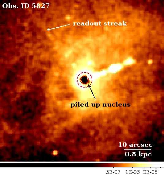
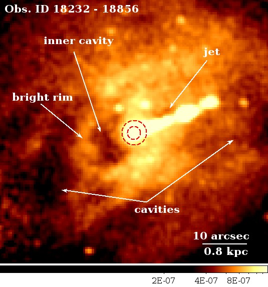
Figure 1: Exposure-corrected Chandra images for the energy range $0.5-7\rm\;keV$. The Bondi radius at $0.12-0.22\rm\;kpc$ ($1.5-2.8\rm\;arcsec$) is shown by the red dashed circles. Left: Obs. ID 5827 was taken in May 2005, close to the brightness peak of HST-1, and therefore exhibits strong pileup. Nuclear events were so piled up that they exceeded Chandra’s energy cutoff and were not telemetered to the ground, which produced the apparent hole. A readout streak also runs from top left to bottom right. Right: The new deep short frame-time Chandra observation shows a nucleus with at most a few per cent pileup and therefore no significant distortions. The colour bar units are $\rm\thinspace counts\hbox{$\rm\;cm^{-2}\,$}\hbox{$\rm\;s^{-1}\,$}\hbox{$\rm\;pixel^{-1}\,$}$.

The Chandra observations of M87 are affected by varying levels of pileup. Pileup occurs when multiple photons from a bright source arrive in the same detector pixel within a single integration time ($3.1\rm\;s$ for a typical Chandra observation). The photons are detected as a single event with higher energy and a broader charge cloud distribution (see eg. Davis 2001). Therefore, pileup hardens the source spectrum and causes grade migration, where events are misclassified as cosmic rays. In extreme cases, pileup can result in lost flux when events exceed the energy filter cutoff in the satellite and are not telemetered to the ground (Fig. 1 left). Strong pileup of the nucleus occurs in standard $3.1\rm\;s$ frame time observations of M87 ($\sim 80\%$ of events affected in obs. ID 352) and in short $0.4\rm\;s$ frame time observations from $\sim 2003-2010$ when the jet knot HST-1 flared and, at peak, was more than an order of magnitude brighter than the nucleus (Harris et al. 2009). Using pimms, the early short frame time observation in 2000 was determined to have a pileup fraction of only $\sim 6\%$ (obs. ID 1808) whilst the monitoring observations from 2010 to 2012 (obs. ids $11513-14974$) are closer to $\sim 10\%$. The drop in the nuclear brightness by roughly a factor of $2-3$ since 2012 ensures that our large observing program in 2016 has the lowest level of pileup at only a few per cent. The nuclear spectrum is therefore not significantly distorted by pileup in our new analysis. We also later confirmed this by including a statistical treatment of pileup in the marx simulations and finding no significant difference.

2.2.2 Nuclear spectrum

A nuclear spectrum was extracted from each separate observation using a circular region of radius $1\rm\;arcsec$ centred on the nuclear peak. The positioning was determined using sub-pixel event repositioning as described above (section 2). The contribution from the galaxy’s hot atmosphere was subtracted using a background spectrum extracted in a surrounding annulus from $2-4\rm\;arcsec$. However, this assumes that the surface brightness profile for the hot gas is flat over the radial range to the nucleus and that the nuclear PSF contribution to this background region is negligible. The hot gas emission is expected to be $\sim 5\%$ of the total emission within $1\rm\;arcsec$ radius whilst the nuclear PSF is at most a few per cent of the emission from $2-4\rm\;arcsec$ in the new datasets. As noted in section 2.1, the measured nuclear flux may also be marginally increased by emission from HST-1. We analysed the effect of these systematic uncertainties in the nuclear spectral model along with other uncertainties in the PSF subtraction in section 2.3.

The nuclear spectra were fit separately in xspec version 12.9.1 (Arnaud 1996) with an absorbed power law model phabs(zphabs(powerlaw)) over the energy range $0.5-7\rm\;keV$. The Galactic absorption component was fixed to the observed value of $1.94\times 10^{20}\hbox{$\rm\;cm^{-2}\,$}$ (Kalberla et al. 2005) and the redshift of the intrinsic absorption component was fixed to $z=0.0044$. All other parameters were left free and the best-fit values were determined by xspec’s modified version of the C-statistic (Cash 1979; Wachter et al. 1979). The best fit parameters for each observation are shown in Table 1. The pattern of nuclear variability appears consistent with long-term monitoring studies of X-ray variability in M87. Harris et al. (2009) characterized the nuclear variability as ‘flickering’, where large amplitude variations in flux are seen on short sampling times and smaller amplitude variations are observed on longer sampling times. Whilst the nuclear flux varies significantly between the separate observations, the spectral index and intrinsic absorption are consistent within the uncertainties. This is consistent with the variability found for other low luminosity AGN at the centre of clusters (eg. Russell et al. 2013). The nuclear spectra from the large program datasets could therefore be fitted together in xspec and this best-fit model was used as the basis of the ChaRT simulation.

2.2.3 ChaRT and marx

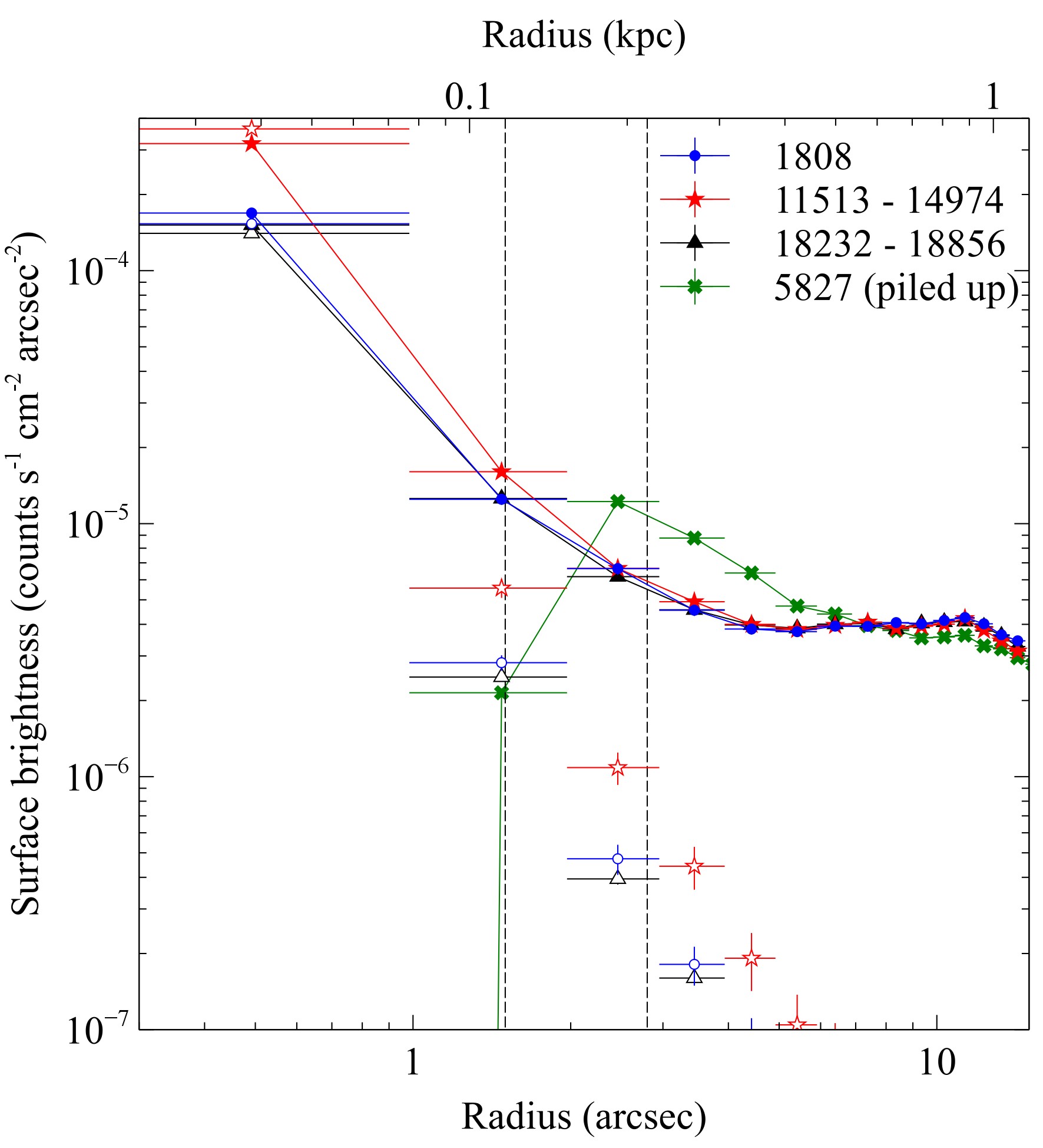
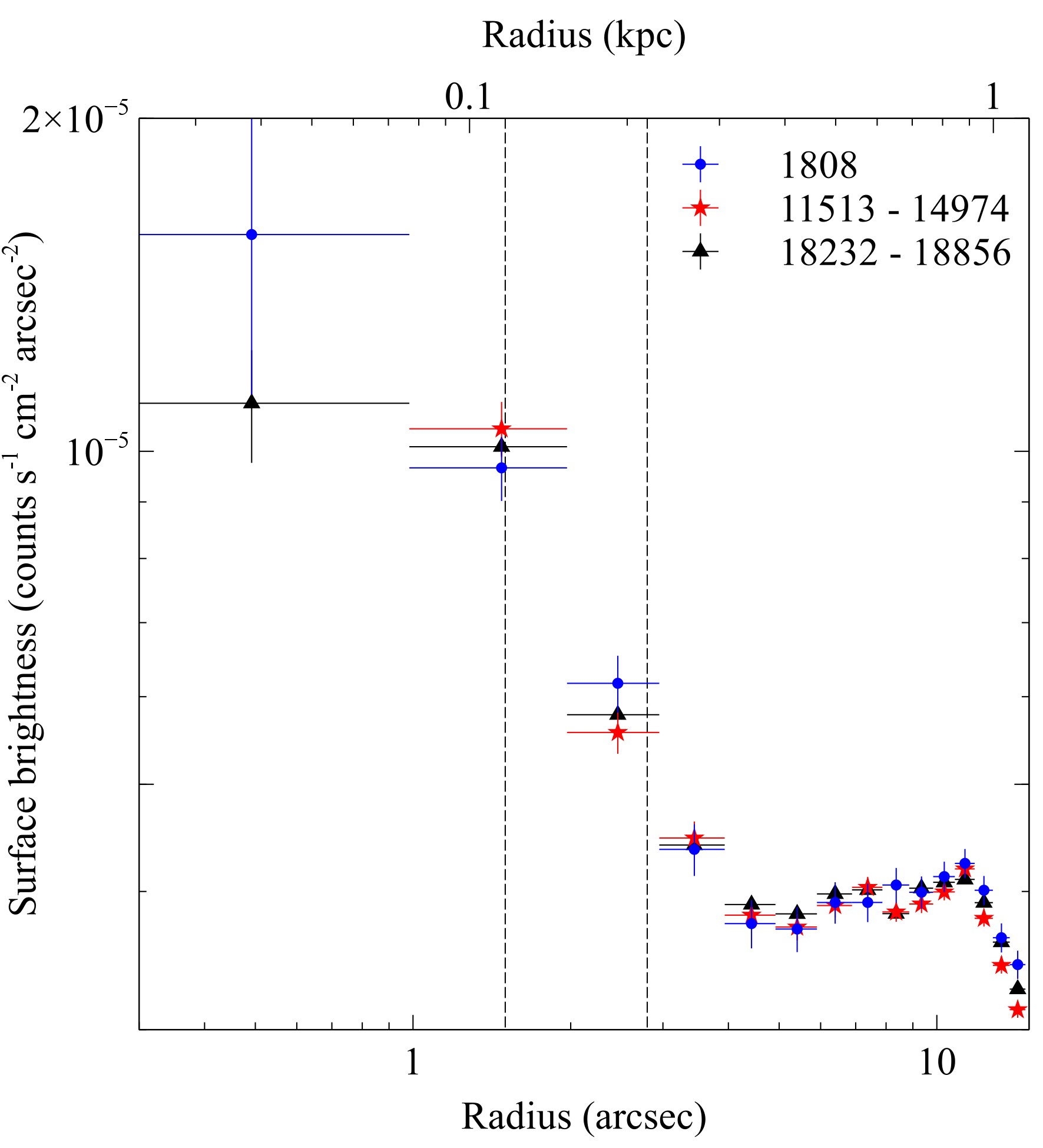
Figure 2: Left: Background-subtracted surface brightness profiles in the energy range $0.5-7\rm\;keV$ for obs. ID 1808, summed obs. IDs 11513 to 14974 and summed obs. IDs 18232 to 18856 (solid points) together with the corresponding ChaRT/marx simulation of the nuclear PSF (open points). Obs. ID 5827 is also shown for comparison. This observation was taken in 2005 with a regular $3.1\rm\;s$ frame time and therefore the nucleus is strongly piled up. Events at the centre exceeded the energy filter cutoff and were not telemetered to the ground from the satellite, which produces the sudden drop in surface brightness within $2\rm\;arcsec$. Right: Surface brightness profiles for the extended hot gas emission where the nuclear PSF has been subtracted from each observation. The radial range for the classical Bondi radius lies between the vertical dashed lines. The profiles were extracted in a sector from $90$ to $330^{\circ}$, which excluded the jet knot emission. The increase in surface brightness at a radius of $10\rm\;arcsec$ is instead due to the inner cavity’s rim. Note that vertical error bars are plotted for all points but in some cases are too small to see.

The ChaRT interface to the SAOTrace code was used to trace rays through the Chandra mirrors and marx then projected these rays onto the detector. SAOTrace was developed as a key calibration tool by the Chandra X-ray Center and provides the most accurate PSF at any off-axis angle and at any energy (eg. Jerius et al. 1995; Jerius et al. 2000; Jerius 2002). Multiple ray-traces were used to produce a total simulation exposure that was an order of magnitude deeper than the observation and thereby ensure good photon statistics. marx version 5.3.2 was used to combine these separate ray-traces, project them onto the ACIS-S detector and apply the appropriate instrumental response (Davis et al. 2012). Following Russell et al. (2015), we also used marx to determine a correction factor for the total flux of the PSF simulation that accounts for the fraction of the PSF lying beyond $1\rm\;arcsec$ radius and, for earlier datasets, the low level of pileup. The output simulated events file from marx was used to produce simulated images and spectra of the nuclear PSF and thereby subtract the nuclear contribution from radial profiles of the extended gas properties.

2.3 Subtraction of the nuclear PSF

The nuclear and jet knot brightness vary significantly over the 16 year span of the M87 observations in Table 1. However, if our method subtracts this emission accurately, the surface brightness of the remaining extended hot gas emission should be consistent within the uncertainties. Exposure-corrected images were produced from the simulated events file for the energy bands $0.5-7\rm\;keV$, $0.5-2\rm\;keV$ and $2-7\rm\;keV$ with spectral weighting given by the best-fit nuclear spectral model (section 2.2.2). Surface brightness profiles for the simulated PSF were extracted from these images using concentric annuli with $1\rm\;arcsec$ width. These simulated surface brightness profiles were compared with, and subtracted from, observed surface brightness profiles generated from a merged, exposure-corrected image (obs. IDs $18232-18856$). The X-ray background emission was also subtracted from the observed datasets using blank sky background images for the corresponding energy range (section 2). This analysis was repeated for the stacked monitoring observations (obs. IDs $11513-14974$) and the earliest short frame-time dataset (obs. ID 1808). Each had a corresponding nuclear PSF simulation. Fig. 2 compares observed, simulated and PSF-subtracted surface brightness profiles for three epochs. In summary, the PSF-subtracted profiles are consistent within the uncertainties for radii $>1\rm\;arcsec$. Therefore, this method produces a reliable PSF subtraction over this radial range.

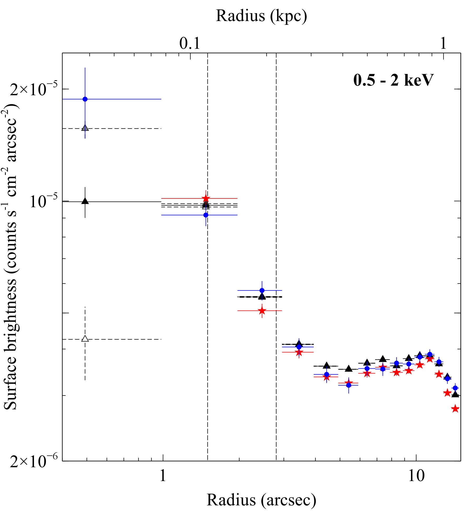
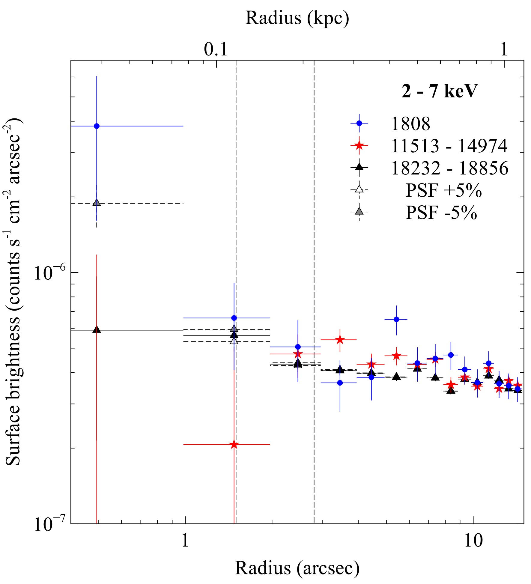
Figure 3: PSF-subtracted surface brightness profiles in two energy bands, $0.5-2\rm\;keV$ and $2-7\rm\;keV$, for the obs. IDs specified in Fig. 2. The impact of under or oversubtracting the PSF simulation by 5% is shown for obs. IDs 18232-18856 by the grey and open points, respectively. The radial range for the classical Bondi radius lies between the vertical dashed lines.

Fig. 3 compares the PSF-subtracted surface brightness profiles for soft and hard energy bands. The temperature of the hot atmosphere at the centre of M87 is $\sim 1\rm\;keV$. This therefore predominantly emits in the soft energy band (Di Matteo et al. 2003; Forman et al. 2005; Million et al. 2010). This gas forms dense, clumpy structures at the galaxy’s centre. The extended emission in the hard energy band from $2-7\rm\;keV$ is dominated by projected emission at large radii, which doesn’t exhibit strong spatial variations on $\sim\rm\;kpc$ scales at the galaxy centre. Therefore, in the absence of nuclear emission, we would expect the hard band surface brightness profile to be close to flat whilst the soft band image has a steeper gradient that traces the low temperature gas at the galaxy centre. The nuclear PSF is a significant emission component in both energy bands within a few arcsec radius. However, when it is correctly subtracted, the hard band surface brightness profile should be roughly flat. A steep decline in surface brightness within a few arcsec radius would indicate a clear oversubtraction, whilst a steep increase would indicate an undersubtraction. Fig. 3 shows that the hard band surface brightness gradient is shallow with no strong variation within a few arcsec of the nucleus. The soft and hard band profiles are also consistent over all three epochs, which suggests that the method is robust.

When the total flux of the optimum PSF simulation is increased by 5 per cent, the $2-7\rm\;keV$ flux within $1\rm\;arcsec$ radius then drops below zero at $-7\pm 4\times 10^{-7}\hbox{$\rm\thinspace counts\hbox{$\rm\;cm^{-2}\,$}\hbox{$\rm\;s^{-1}\,$}\hbox{$\rm\;arcsec^{-2}\,$}$}$. Alternatively, if the flux of the PSF simulation is decreased by 5 per cent, the $2-7\rm\;keV$ flux within $1\rm\;arcsec$ radius is strongly peaked at $1.9\pm 0.4\times 10^{-6}\hbox{$\rm\thinspace counts\hbox{$\rm\;cm^{-2}\,$}\hbox{$\rm\;s^{-1}\,$}\hbox{$\rm\;arcsec^{-2}\,$}$}$. We therefore estimate uncertainties on the total flux of the nuclear PSF simulation to be less than 5 per cent. This uncertainty is ultimately due to the difficulty in cleanly separating the nuclear emission from the background extended emission. We tested the impact of variations in the subtracted PSF normalization by $\pm 5\%$ on the best-fit cluster model parameters. The resulting systematic uncertainties were found to be insignificant compared to the statistical uncertainties. The nuclear PSF subtraction is therefore sufficiently accurate for this analysis.

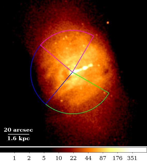
Figure 4: Summed image for obs. IDs 18232 to 18856 showing the N, E and S sectors used. The colour bar has units of counts.

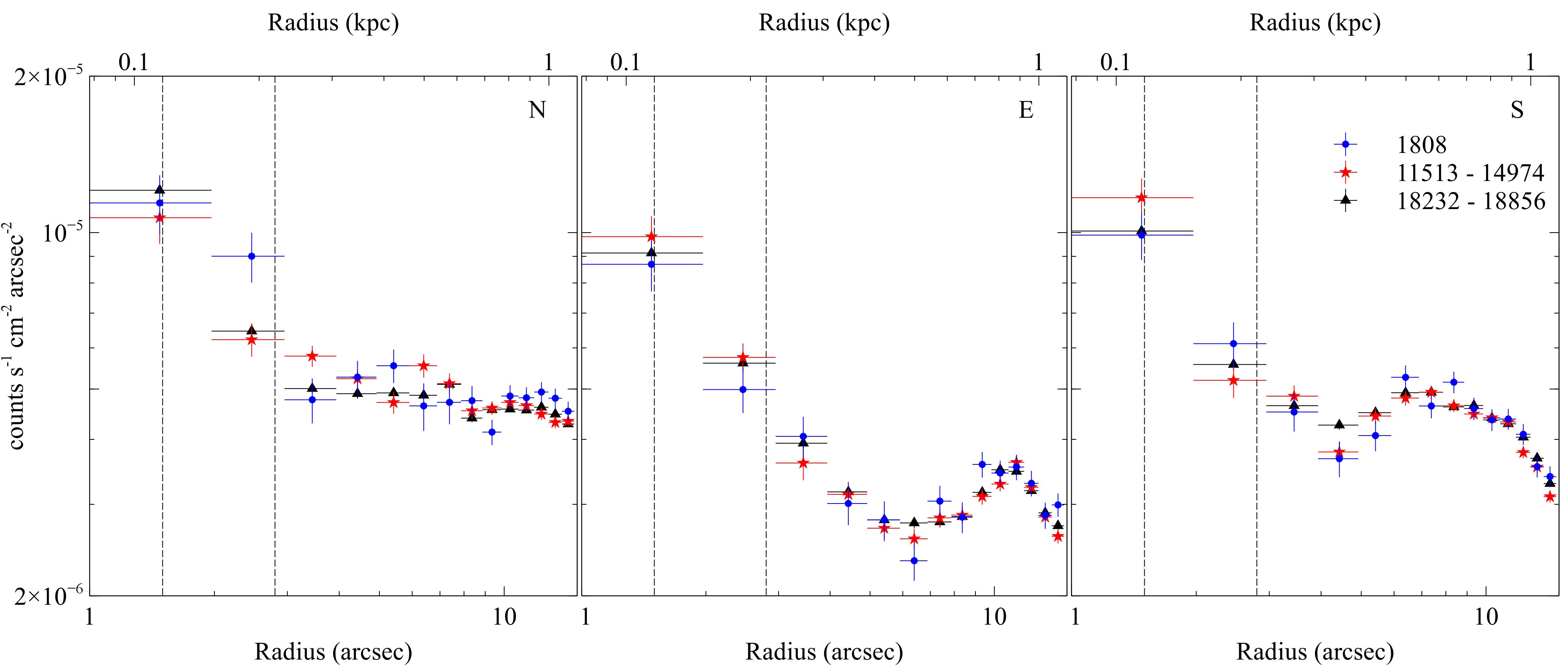
Figure 5: PSF-subtracted surface brightness profiles in three sectors (Fig. 4) for the obs. IDs specified in Fig. 2. The radial range for the classical Bondi radius lies between the vertical dashed lines. The drop in surface brightness due to the inner cavity can be clearly seen from $\sim 4-10\rm\;arcsec$ in the E and S sectors.

The gas properties of the galaxy’s hot atmosphere were also extracted in three sectors that together covered the angular range $90-330^{\circ}$ avoiding the jet (Fig. 4). Within this range, the sectors were selected on the morphology of the extended emission, particularly the cavity to the E of the nucleus from $\sim 4$ to $10\rm\;arcsec$ radius and the soft X-ray filaments. Fig. 5 shows that the PSF-subtracted surface brightness profiles are also consistent across the three epochs in each of the sectors. The PSF simulation was therefore accurately centred on the observed PSF during the subtraction by the subpixel event repositioning (section 2). Although not shown, the PSF-subtracted surface brightness profiles in each sector are also consistent when split into soft and hard energy bands as discussed above.

2.4 Spectral analysis

Spectra were extracted from each observation (obs. IDs $18232-18856$) in concentric annuli from $60-330^{\circ}$ and in sectors from $60-140^{\circ}$ (N sector), $140-230^{\circ}$ (E sector) and $230-330^{\circ}$ (S sector), where angles are measured anti-clockwise from W (Fig. 4). Background spectra were extracted from the blank sky backgrounds that had been generated for each dataset (section 2). Observations $18232-18856$ were taken over a period of only a few months and the spatial regions analysed are all within the central $30\rm\;arcsec$ and therefore have similar responses. Spectra from the same spatial region were therefore summed together and the response files were averaged according to a weighting determined from the fraction of the total counts in each observation. The use of summed spectra was also verified by comparing the best-fit parameters with those determined when fitting the individual spectra simultaneously in xspec. The best-fit results in each case were found to be consistent within the uncertainties.

The short frame-time observations were taken using a 1/8th subarray to preserve observing efficiency. Therefore the field of view was limited to $1\times 8\rm\;arcmin$. We increased the radial range for the analysis by extracting spectra from $14-300\rm\;arcsec$ in obs. ID 352, which is only strongly piled up within the central few arcsec of the nucleus. Spectra were deprojected with a modified version of the model-independent deprojection routine dsdeproj, which assumes spherical symmetry and employs a geometrical procedure to subtract off the projected emission. This version of dsdeproj includes a correction for the difference in effective area between the summed spectra and those extracted from obs. ID 352 (Sanders & Fabian 2007; Russell et al. 2008; Russell et al. 2015). The spectra were analysed over the energy range $0.5-7\rm\;keV$ and counts were grouped for at least 25 per spectral bin.

The deprojected spectra were fitted in xspec version 12.9.1 (Arnaud 1996) with absorbed one, two and three component vapec models (Smith et al. 2001). The redshift was fixed to $z=0.0044$ and the Galactic absorption was fixed to $n_{\mathrm{H}}=1.94\times 10^{20}\hbox{$\rm\;cm^{-2}\,$}$. The $\chi^{2}$ statistic was used to determine the best-fit model. The metal abundances were fixed relative to Fe according to the radial profiles for Fe, Si, S, Ar, Ca, Ne, Mg and Ni measured by Million et al. (2011) from the archival Chandra observations. The C, N and O abundances were also fixed relative to Fe according to the XMM-Newton RGS results of Werner et al. (2006).

The XMM RGS results were extracted from a $1.1\rm\;arcmin$ wide strip and the Chandra analysis excluded the inner core and the X-ray bright arms therefore it was not clear whether the measured abundances were applicable for the multi-phase gas within a radius of $1\rm\;kpc$. However, in the existing data, it was not possible to constrain individual metal abundances in the cooler gas component, even when fixing the abundances of the spatially coincident hotter component. We have therefore assumed no strong variation in the metal abundances relative to iron between the multiple temperature components, which is broadly supported by these earlier analyses. The abundances were measured throughout relative to the protosolar measurements from Lodders (2003).

An additional absorbed power-law component was used to account for the nuclear emission in spectra extracted within a radius of $6\rm\;arcsec$ ($0.5\rm\;kpc$). The parameters were fixed to values determined from the PSF simulations. Spectra were extracted from the simulations using identical regions, deprojected and then fit in xspec with an absorbed power-law model phabs(zphabs(powerlaw)). The Galactic column density and redshift were fixed but all other parameters were left free when fitting to the simulated spectra. The best-fit parameters from the simulation were then fixed in the nuclear emission component used to model the observed spectra. These parameters must be fixed when modelling the observed spectra to ensure that the PSF contribution is not incorrectly interpreted as a hot thermal component when a multi-temperature model is used.

The temperature and normalization of each thermal vapec component were left free and the iron abundance was left free for spectra extracted from larger radial bins. For the multi-temperature models, the iron abundance was tied between the different components. The densities were calculated from the vapec normalizations and assumed pressure equilibrium between the multi-temperature components.

3 Results

By simulating and modelling the spectral contribution of the bright nucleus, the temperature and density structure of the galaxy’s hot atmosphere could be extracted in sectors to a radius of $1\rm\;arcsec$ ($78\rm\;pc$), which is within the SMBH’s gravitational sphere of influence. Fig. 6 shows an analysis in large radial bins for annuli from $60-330^{\circ}$ where up to three temperature components were included. The iron abundance was left as a free parameter. The hot gas is clearly multi-phase at the galaxy centre with components at $1.6^{+0.3}_{-0.2}\rm\;keV$, $0.7\pm 0.2\rm\;keV$ and $0.19\pm 0.03\rm\;keV$. The temperature of all three components decreases, or is approximately constant, toward the nucleus. The electron density increases steadily with decreasing radius and the density of the cooler component peaks above $1\hbox{$\rm\;cm^{-3}\,$}$. Note that the increase in density in the outermost radial bin is an artefact of deprojection.

The iron abundance peaks at $\sim 2\hbox{$\thinspace\mathrm{Z}_{\odot}$}$ at a radius of $2\rm\;kpc$ ($25\rm\;arcsec$) and then decreases towards the galaxy centre to $\sim 0.7\hbox{$\thinspace\mathrm{Z}_{\odot}$}$. This abundance drop was previously found in XMM-Newton observations (Böhringer et al. 2001) and does not appear to be due to the Fe bias that typically occurs when a single temperature model is fitted to the spectrum of a multi-temperature medium (eg. Buote 2000) or to resonant scattering (Mathews et al. 2001; Sanders & Fabian 2006). The metallicity was fixed according to this profile in our subsequent analysis.

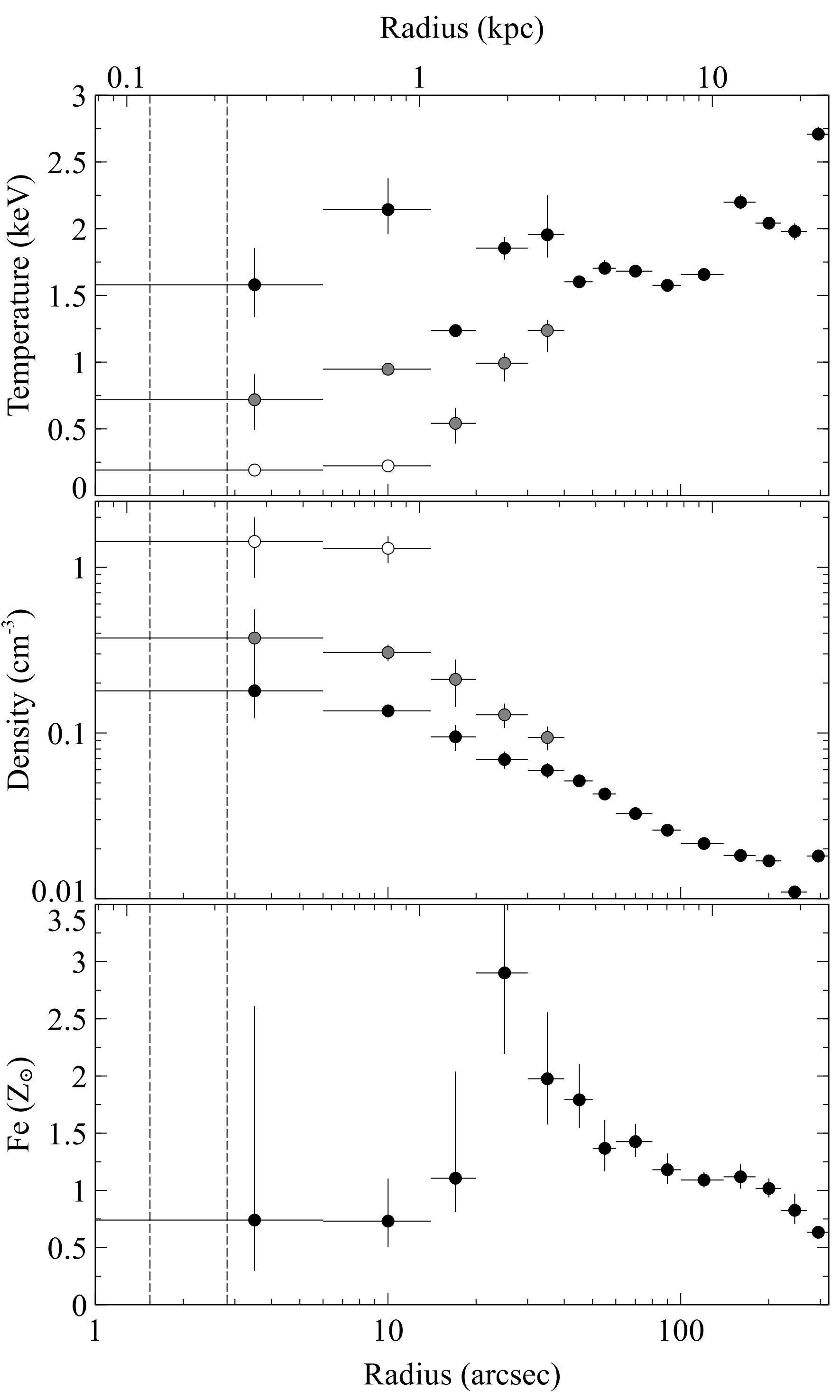
Figure 6: Deprojected temperature, electron density and Fe abundance profiles for full annuli in broad radial bins. Additional spectral components were added where these significantly improved the best-fit result and these are shown as grey and white points. The radial range for the classical Bondi radius lies between the vertical dashed lines.

3.1 Multi-phase gas structure within the Bondi radius

These annuli with broad radial binning were sub-divided into $1-2\rm\;arcsec$ widths in N, E and S sectors to resolve the temperature and density structure within the Bondi radius (Fig. 4 and Table 2). The N sector covers the brightest loops of soft X-ray emission that are coincident with H$\alpha$ filaments and extend $\sim 20\rm\;arcsec$ north of the nucleus (eg. Sparks et al. 1993; Sparks et al. 2004). The E sector encompasses the inner cavity and the knotty complex of soft X-ray and H$\alpha$ emission at a radius of $\sim 35\rm\;arcsec$ that coincides with the outer edge of the radio lobe (Sparks et al. 1993). The S sector covers the SW corner of the inner cavity and contains bright soft X-ray emission similar to the N sector but is relatively free of H$\alpha$ emission. The SW corner of the inner cavity extends to the S of the nucleus. It was therefore not possible to exclude this cavity from the S sector whilst also ensuring that the innermost region was at least $1\rm\;arcsec$ across to match Chandra’s spatial resolution. We therefore positioned the boundary between the E and S sectors to provide comparable deprojected count rates in the inner regions and therefore similar parameter constraints.

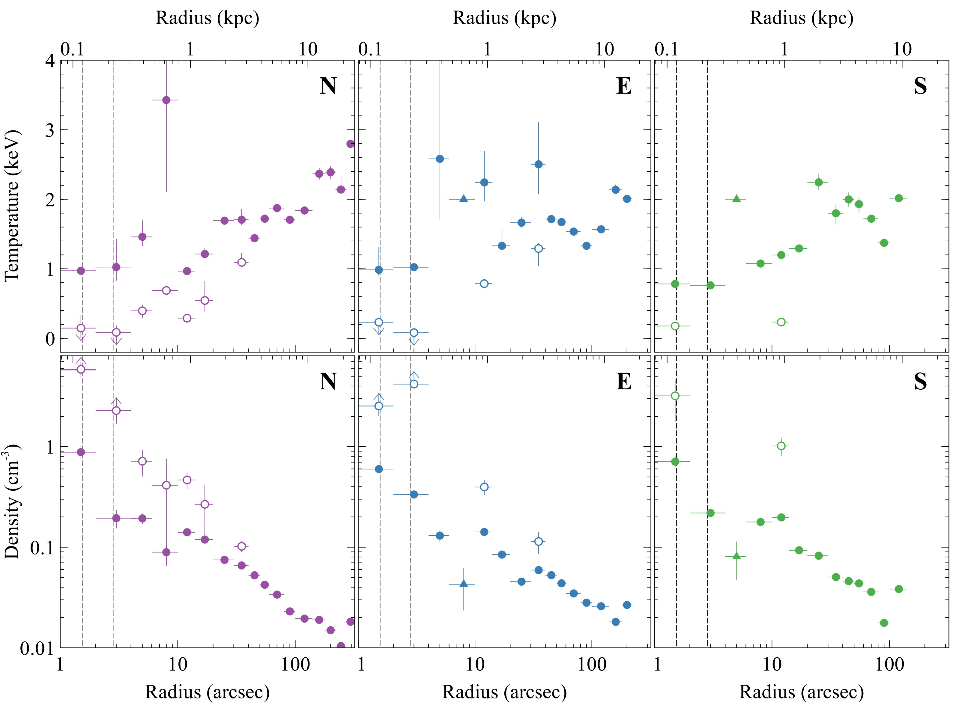
Figure 7: Deprojected temperature and electron density profiles in the N, E and S sectors (Fig. 4). An additional spectral component was added where this significantly improved the best-fit result (open points). Regions affected by the cavity where the temperature was fixed are shown by the triangles. The radial range for the classical Bondi radius lies between the vertical dashed lines.

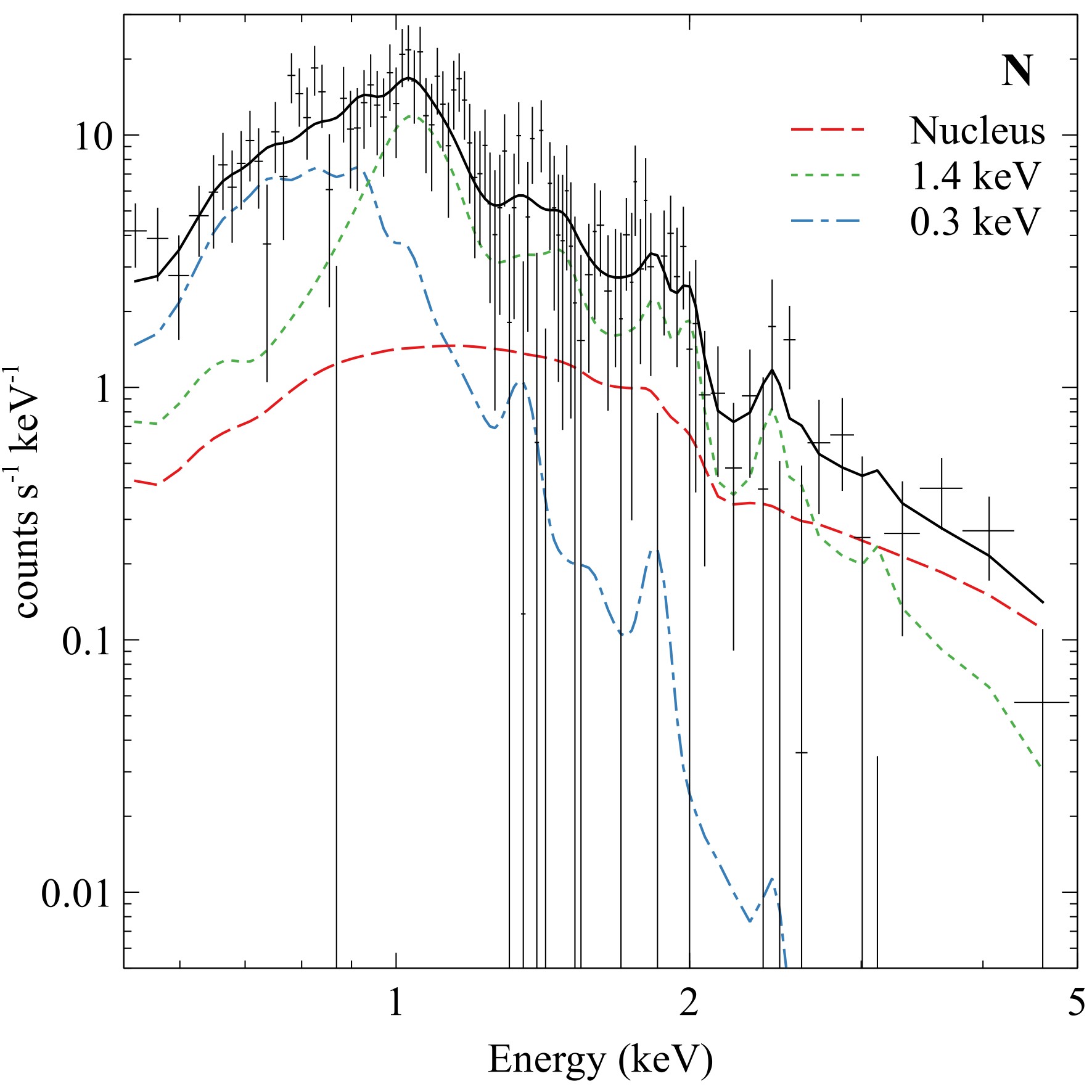
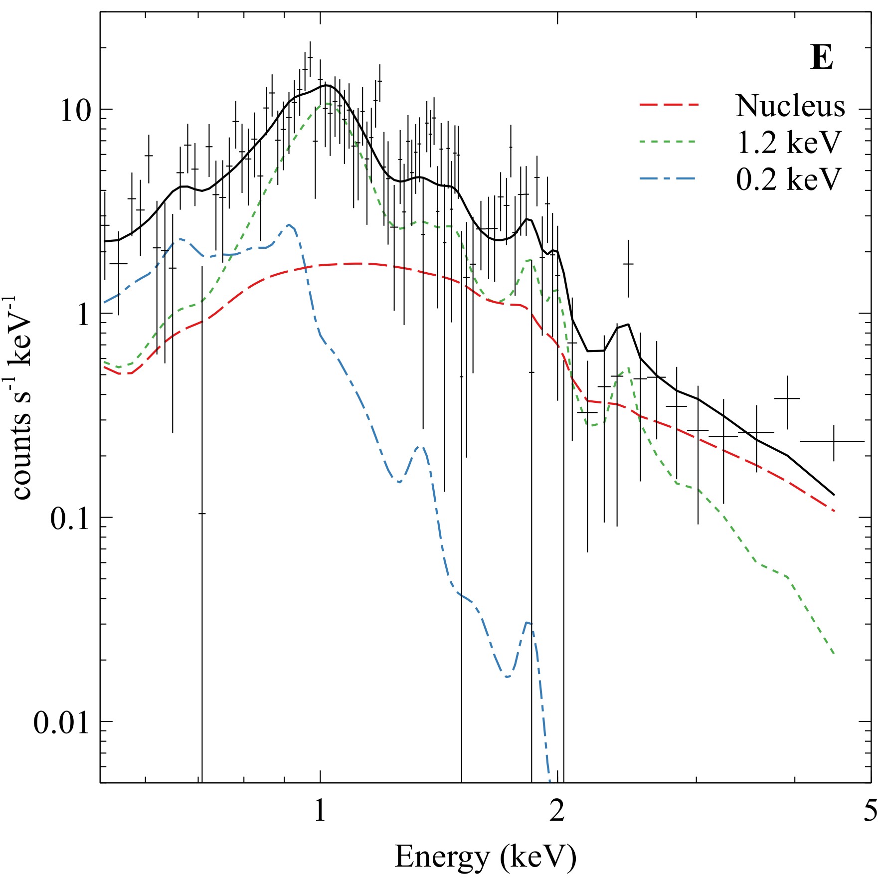
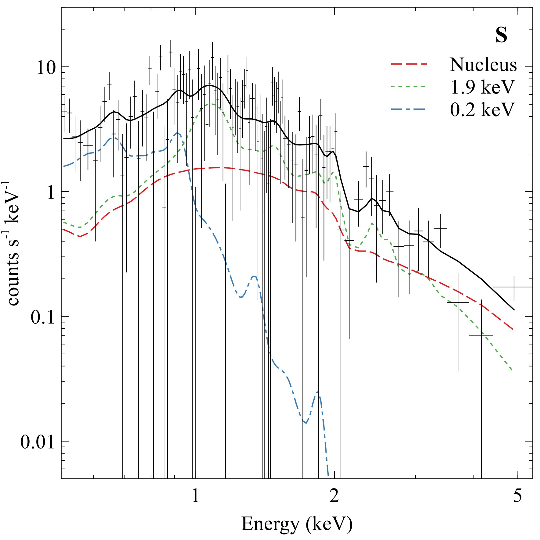
Figure 8: Deprojected spectra with best-fit models for the innermost region ($1-6\rm\;arcsec$) in the N (left), E (centre) and S (right) sectors. The total best-fit model is shown by the black solid line and each component is shown by a dashed or dotted line. Although the best-fit models can be improved if some metallicity parameters are left free, particularly Mg and Si, the best-fit values are very poorly constrained.

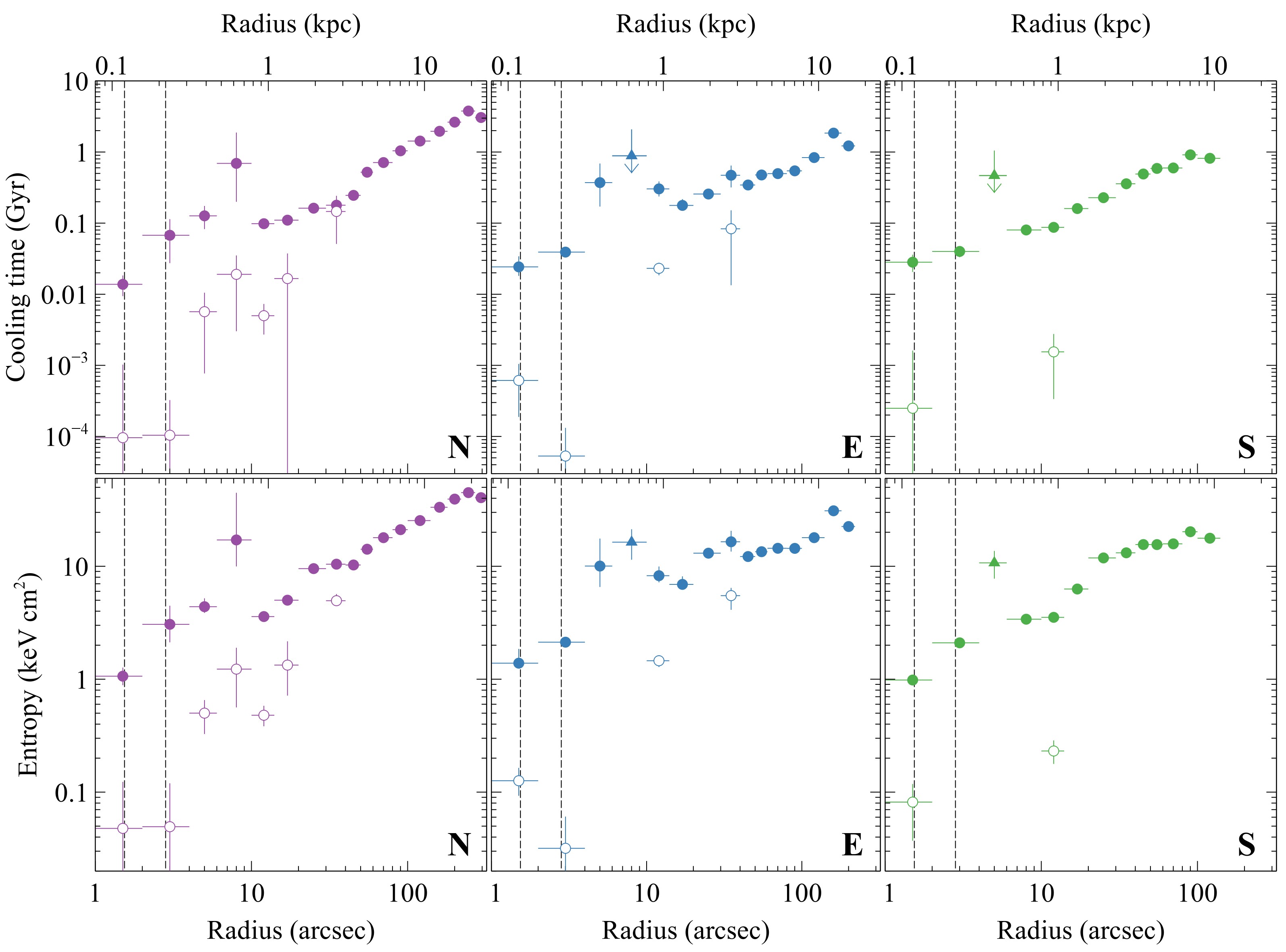
Figure 9: Deprojected cooling time and entropy profiles in the N, E and S sectors (Fig. 4). An additional spectral component was added where this significantly improved the best-fit result (open points). Regions affected by the cavity where the temperature was fixed are shown by the triangles. The radial range for the classical Bondi radius lies between the vertical dashed lines. Within the Bondi radius, a vmcflow model provides a similarly good fit.

Fig. 7 shows that the multi-temperature structure is detected within all sectors in the central kpc with components at $0.2\rm\;keV$ and $0.8-1\rm\;keV$. The temperature structure within the central few arcsec is remarkably symmetric about the nucleus, despite the inner cavity structure. Whilst the additional $0.2\rm\;keV$ components significantly improve the best-fit result, their specific temperature and density values are poorly constrained by Chandra’s $0.5-7\rm\;keV$ energy range and are therefore shown as upper and lower limits in Fig. 7, respectively. No evidence was found for a temperature increase within the Bondi radius due to the gravitational influence of the SMBH. Instead, the lowest temperature gas is located closest to the nucleus.

The metallicity was fixed according to the profiles found for spectra extracted from annuli from $60-330^{\circ}$ (section 3). We note that, if the Fe abundance is left as a free parameter for spectra extracted in sectors, the corresponding metallicity profiles are similar between these sectors, particularly within the central few kpc. However, given the large uncertainties within $\sim 10\rm\;arcsec$, we also investigated whether possible variations of $\pm 0.3\hbox{$\thinspace\mathrm{Z}_{\odot}$}$ could affect the derived gas properties. This level of uncertainty produced negligible changes in the temperature values for each component but shifts of $\sim 15\%$ and $\sim 20\%$ in the density values for the higher and lower temperature components, respectively. Therefore, whilst the temperature structure is unaffected, strong variations in the metallicity on scales of $\sim 100\rm\;pc$ could affect the measured density gradient within the Bondi radius.

Fig. 8 shows the deprojected spectra and best-fit models for regions covering $1-6\rm\;arcsec$ in the N, E and S sectors. For the N sector, the fit statistic decreases from $\chi^{2}=159$ with 100 degrees of freedom for one vapec component to $\chi^{2}=98$ with 98 degrees of freedom for two vapec components. The additional low temperature component at $0.30\pm 0.04\rm\;keV$ is therefore clearly required over a single vapec model and fits the excess at $\sim 0.7\rm\;keV$, which is likely due to O emission (eg. Sakelliou et al. 2002; Werner et al. 2006). For the E sector, the fit statistic decreases from $\chi^{2}=129$ with 95 degrees of freedom for one vapec component to $\chi^{2}=109$ with 93 degrees of freedom for two vapec components. Similarly, for the S sector, the fit statistic decreases from $\chi^{2}=154$ with 100 degrees of freedom for one vapec component to $\chi^{2}=103$ with 98 degrees of freedom for two vapec components. The excess emission at low energies above a $\sim 1\rm\;keV$ model is less prominent than in the N sector but still significant. We note that the best-fit results can be improved if some metallicity parameters are left free, such as Mg and Si, which have prominent emission lines at $1.3$ and $1.9\rm\;keV$ respectively. However, the best-fit values are very poorly constrained.

For the innermost regions within the Bondi radius, the deprojected spectra can also be equivalently fit with an absorbed cooling flow model phabs(vmcflow) with no vapec components (Mushotzky & Szymkowiak 1988; Johnstone et al. 1992). For the N sector, the best-fit cooling flow model has $\chi^{2}=57.2$ for 44 degrees of freedom compared to the two vapec component model with $\chi^{2}=55.2$ for 43 degrees of freedom. The abundances for both models were fixed to the values determined in section 3. The best-fit upper temperature parameter for the vmcflow model was $1.5\pm 0.1\rm\;keV$. The best-fit lower temperature parameter reached the model’s lower limit at $0.08\rm\;keV$ with an upper limit of $<0.4\rm\;keV$. The mass deposition rate was $0.028^{+0.002}_{-0.003}\hbox{$\hbox{$\rm\thinspace M_{\odot}$}\rm\;yr^{-1}\,$}$. Similar results were obtained for the innermost deprojected spectra in the E and S sectors. The emission within the Bondi radius is therefore equivalently consistent with a cooling flow in all three sectors with gas cooling down out of the X-ray band from $1-1.5\rm\;keV$ at a rate of $\sim 0.03\hbox{$\hbox{$\rm\thinspace M_{\odot}$}\rm\;yr^{-1}\,$}$.

Detection of the low temperature X-ray gas could be affected by variations in the Galactic absorption or the growing layer of molecular contaminant on the ACIS optical blocking filter. However, it is unlikely that strong variations in either of these effects would only occur coincident with the Bondi sphere. Lieu et al. (1996) found a smooth distribution of Hi with $n_{\mathrm{H}}\sim\left(1.8-2.1\right)\times 10^{20}\hbox{$\rm\;cm^{-2}\,$}$ and limited spatial variation over the field of M87 (also Kalberla et al. 2005). Similarly, whilst the molecular contaminant is not uniformly distributed with increased depth at the edges of the filters, strong spatial variation just within the Bondi sphere at the centre of the chip is unlikely. Although it is possible that the deprojection routine could compound effective area uncertainties into the spectra for the central regions, due to the limited 1/8th field of view of the short frame-time observations, the majority of the projected emission was subtracted with obs. ID 352 (section 2.4), which was taken early in the Chandra mission before significant contaminant buildup. Given the brighter nuclear emission and shorter exposure times, it was unfortunately not possible to verify the detection of low temperature gas in the earlier short frame-time observations of M87.

On larger scales, the multi-temperature X-ray structure extends to $\sim 20\rm\;arcsec$ radius in the N sector, which is consistent with the extent of the ionized gas filaments (eg. Sparks et al. 1993; Sparks et al. 2004). In the E sector, the low temperature components are detected around the periphery of the inner cavity. The S sector is largely free of ionized gas and we similarly find only limited low X-ray temperature gas beyond that detected within the Bondi radius. The narrow radial binning produced two regions that were strongly affected by the X-ray surface brightness depression of the inner radio bubble. The corresponding deprojected spectra had very low numbers of photons therefore the temperature was fixed in these regions to that of the projected emission at $2\rm\;keV$ (shown as triangles in Fig. 7). These radial bins are included in the figures for reference but were not considered further in our analysis.

The low temperature component likely consists of rapidly cooling blobs and filaments within the hotter, volume-filling component at $1-2\rm\;keV$. The filling fraction of the cold gas is $5-20\%$ within the Bondi sphere and roughly a few per cent at larger radii. By assuming that the two gas phases are in pressure equilibrium, and ignoring magnetic pressure, the gas density of each component can be calculated. The density of both temperature components continues to rise towards the nucleus. The density of the hotter component peaks at $0.9\pm 0.1\hbox{$\rm\;cm^{-3}\,$}$ in the N sector within the Bondi radius. The gas density in the other sectors is similarly high within the Bondi radius and peaks at $0.60\pm 0.05\hbox{$\rm\;cm^{-3}\,$}$ and $0.71\pm 0.09\hbox{$\rm\;cm^{-3}\,$}$ in the E and S sectors, respectively. Although poorly constrained by Chandra’s energy range, the cooler component likely reaches densities at least a factor of a few greater than this at $>2\hbox{$\rm\;cm^{-3}\,$}$.

The radiative cooling time, $t_{\mathrm{cool}}=(5/2)nkT/n^{2}\Lambda$, and the entropy, $S=T/n_{\mathrm{e}}^{2/3}$, of each component were calculated from the deprojected temperature and density profiles. Note that this definition of cooling time is $5/3$ times that used in Russell et al. (2015). Fig. 9 shows the radiative cooling time and entropy profiles in each of the three sectors. For the higher temperature component, the cooling time and entropy continue to decline to the Bondi radius to $\sim 0.02\rm\;Gyr$ and $\sim 1\hbox{$\rm\;keV\rm\;cm^{2}\,$}$, respectively. The cooling time of the low temperature gas drops to only $0.1-0.5\rm\;Myr$. This is comparable to the free fall time at this radius, which can be determined from models of the mass distribution in M87 that include the stellar mass, the dark matter halo and the central supermassive black hole (eg. Gebhardt & Thomas 2009). The entropy of this component is equivalently below $0.1\hbox{$\rm\;keV\rm\;cm^{2}\,$}$.

3.2 Density gradient within the Bondi radius

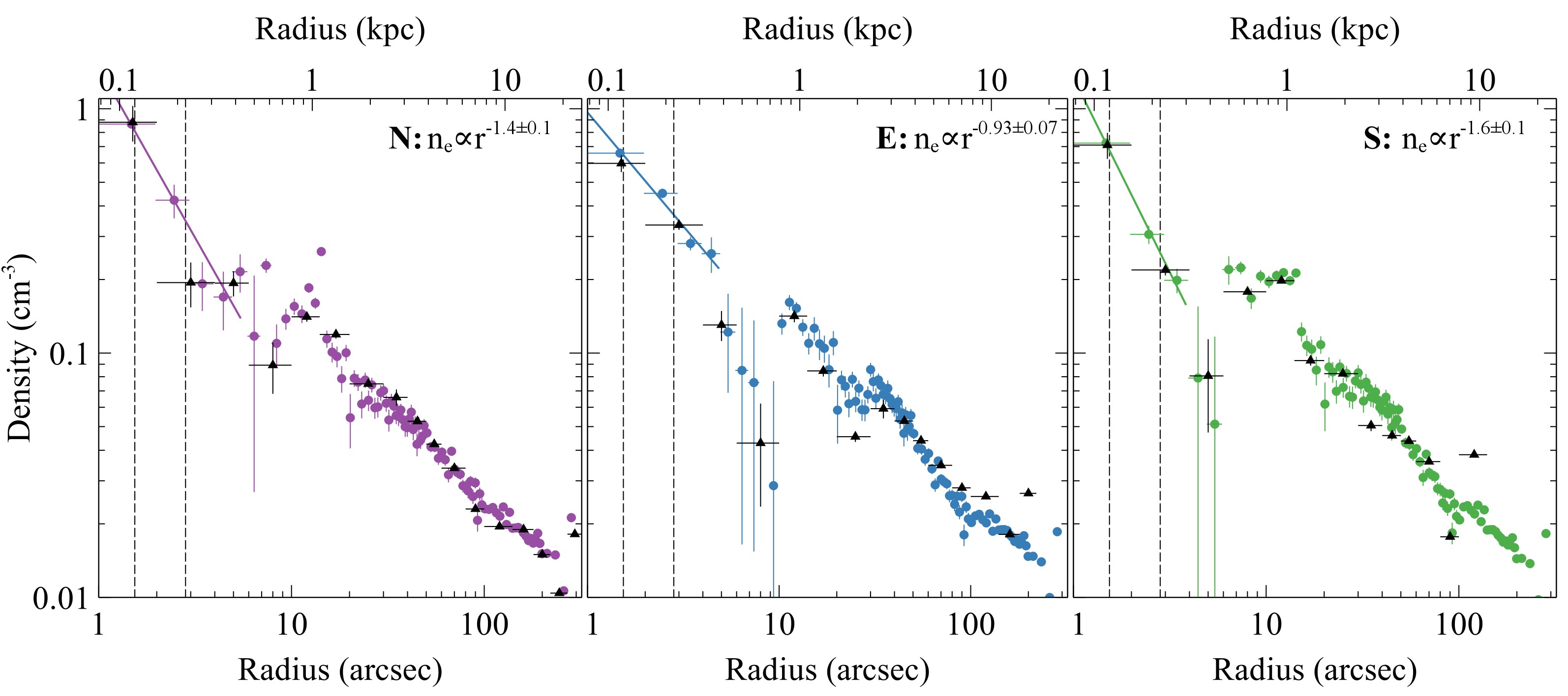
Figure 10: Deprojected electron density profiles with finer radial binning and the original binning (black triangles) for the N, E and S sectors (Fig. 4). The solid lines show the best-fit powerlaw models for the hot gas within the Bondi radius. The radial range for the classical Bondi radius lies between the vertical dashed lines.

Density profiles with finer radial binning were also generated from the PSF and background subtracted surface brightness profiles in each sector. Following eg. Cavagnolo et al. (2009), this technique incorporates temperature and metallicity variations determined from the spectral fitting results. Fig. 10 shows the density profiles in each sector for the hotter volume filling component (see also Table 3). The density values determined in narrower radial bins are consistent with our previous results from spectral fitting. The density gradient across the Bondi radius was determined by fitting a power-law model to the density profile in each sector using data points within a radius of $4-5\rm\;arcsec$ ($0.3-0.4\rm\;kpc$). This region was selected to cover the symmetric structure about the nucleus and avoid the inner cavity. Note that this covered only 5 radial points in the N sector, 4 points in the E sector and 3 points in the S sector. The best-fit powerlaw slopes, $n_{\mathrm{e}}{\propto}r^{\alpha}$, in the N, E and S sectors are $\alpha=-1.4\pm 0.1$, $\alpha=-0.93\pm 0.07$ and $-1.6\pm 0.1$, respectively. The E sector along the jet has a significantly flatter density gradient than the N and S sectors that are perpendicular to the jet. Russell et al. (2015) previously determined a powerlaw slope of $-1.2\pm 0.2$ for circular annuli, which is roughly consistent with our new results. The shallower observations utilized in this earlier work prevented us from excluding the inner cavity or separating the density profiles into separate sectors.

3.3 Bondi accretion rate

The Bondi model states that the galaxy’s hot gas atmosphere will be accreted by the SMBH if it falls within the Bondi radius, where the gravitational potential of the SMBH dominates over the thermal energy of the gas (Bondi 1952). This model assumes spherical accretion onto a point mass, an absorbing inner boundary condition and negligable angular momentum. The Bondi rate can then be calculated from the gas electron density, $n_{\mathrm{e}}$, and temperature, $T$, and the mass of the black hole, $M_{\mathrm{BH}}$. The Bondi accretion rate is given by

$$\dot{M}_{\mathrm{B}}=\frac{4\pi\lambda\left(GM_{\mathrm{BH}}\right)^{2}}{c_{\mathrm{s}}^{3}},$$ (1)

where $c_{\mathrm{s}}$ is the sound speed in the gas and $\lambda$ is dependent on the adiabatic index of the gas. Assuming an adiabatic index $\gamma=5/3$, this coefficient $\lambda=0.25$. The Bondi accretion rate can then be written as

$$\frac{\dot{M}_{\mathrm{B}}}{\hbox{$\hbox{$\rm\thinspace M_{\odot}$}\rm\;yr^{-1}\,$}}=0.012\left(\frac{k_{\mathrm{B}}T}{\mathrm{keV}}\right)^{-3/2}\left(\frac{n_{\mathrm{e}}}{\hbox{$\rm\;cm^{-3}\,$}}\right)\left(\frac{M_{\mathrm{BH}}}{10^{9}\hbox{$\rm\thinspace M_{\odot}$}}\right)^{2},$$ (2)

and the Bondi radius is given by

$$\frac{r_{\mathrm{B}}}{\mathrm{kpc}}=0.031\left(\frac{k_{\mathrm{B}}T}{\mathrm{keV}}\right)^{-1}\left(\frac{M_{\mathrm{BH}}}{10^{9}\hbox{$\rm\thinspace M_{\odot}$}}\right).$$ (3)

Stellar-dynamical and gas-dynamical measurements of the black hole mass at the centre at M87 typically differ by a factor of two and are discrepant at the $2\sigma$ level. From stellar dynamics, Gebhardt et al. (2011) measure $M_{\mathrm{BH}}=\left(6.6\pm 0.4\right)\times 10^{9}\hbox{$\rm\thinspace M_{\odot}$}$ (see also Sargent et al. 1978; Oldham & Auger 2016). Whilst from gas dynamics, Walsh et al. (2013) measure $M_{\mathrm{BH}}=\left(3.5^{+0.9}_{-0.7}\right)\times 10^{9}\hbox{$\rm\thinspace M_{\odot}$}$ (see also Harms et al. 1994; Macchetto et al. 1997). Properties that are dependent on the black hole mass, such as the Bondi radius and Bondi accretion rate, are therefore shown as a range of values that span these two measurements.

For the volume-filling, higher temperature component, the deprojected temperature at the centre of M87 is $0.97^{+0.10}_{-0.04}\rm\;keV$, $0.98^{+0.33}_{-0.08}\rm\;keV$ and $0.78^{+0.06}_{-0.04}\rm\;keV$ in the N, E and S sectors, respectively. The Bondi radius is therefore located at $0.12-0.21\rm\;kpc$ ($1.5-2.7\rm\;arcsec$) in the N and E sectors and $0.14-0.26\rm\;kpc$ ($1.8-3.3\rm\;arcsec$) in the S sector. The Bondi accretion rate is then $0.1-0.5\hbox{$\hbox{$\rm\thinspace M_{\odot}$}\rm\;yr^{-1}\,$}$ for the higher temperature component.

4 Discussion

Our new $300\rm\;ks$, short frame-time dataset for M87 provides a detailed view of the hot gas properties inside the Bondi radius of the SMBH. On these scales, the temperature structure is spherically symmetric about the nucleus with two temperature components at $0.2\rm\;keV$ and $0.8-1\rm\;keV$ detected in all three sectors. The lowest temperature and most rapidly cooling X-ray gas in M87 is therefore located within the Bondi radius. The radio-jet has carved out a series of cavities in the surrounding X-ray gas, each at least few kpc across, that heat the hot atmosphere on these larger scales (eg. Forman et al. 2005, 2007; Forman et al. 2017). Beyond the Bondi sphere, additional low temperature components detected in the hot gas are predominantly located to the N of the nucleus and clearly coincident with the soft X-ray and bright ionized gas filaments. These filaments extend for several kpc to the N and E of the nucleus and are entwined around the buoyant bubbles (eg. Forman et al. 2005, 2007).

The density profiles in each sector plateau at a radius of $0.5-1\rm\;kpc$, around the inner cavity structure, and then rise steeply within the Bondi radius to $\sim 1\hbox{$\rm\;cm^{-3}\,$}$. The N and S sectors have the steepest gradients with $\rho{\propto}r^{-1.5}$. The E sector along the jet axis is significantly shallower with $\rho{\propto}r^{-0.9}$. This structure is consistent with anisotropic outflow along the jet. On larger scales, the density structure clearly varies across the different sectors due to the surface brightness depressions and bright rims of the radio bubbles. Additional higher density, cool gas structures associated with the soft X-ray filaments are embedded within the hotter volume-filling gas and detected to a radius of several kpc. Although the flux of the low temperature component is poorly constrained by Chandra’s energy range, the density is likely to be at least a factor of a few higher at $>2\hbox{$\rm\;cm^{-3}\,$}$. Within the Bondi radius, the gas is rapidly cooling to low temperatures but asymmetries in the density gradient suggest this region is a mixture of steadily inflowing material to the N and S and outflow along the jet axis.

4.1 Gas cooling within the Bondi sphere

The radiative cooling time of the $0.2\rm\;keV$ gas within the Bondi radius is extremely short at $<1\rm\;Myr$, which is similar to the free fall time at this radius. In section 3.1, we showed that deprojected spectra extracted from within the Bondi radius can be fit equivalently by a two temperature thermal model with components at $0.2$ and $1\rm\;keV$ or by a single cooling flow model with gas cooling from $1.5\rm\;keV$ down to the lower limit of $0.08\rm\;keV$. It appears likely that the gas is rapidly cooling down out of the X-ray band within the Bondi radius. The best-fit mass deposition rate within a radius of $2\rm\;arcsec$ ($0.15\rm\;kpc$) is $0.028^{+0.002}_{-0.003}\hbox{$\hbox{$\rm\thinspace M_{\odot}$}\rm\;yr^{-1}\,$}$. This cooling rate is consistent with the XMM-Newton RGS limit on gas cooling below $0.5\rm\;keV$ of $\dot{M}<0.06\hbox{$\hbox{$\rm\thinspace M_{\odot}$}\rm\;yr^{-1}\,$}$ (Werner et al. 2010), which was determined in a $1.1\rm\;arcmin$ wide aperture ($5.2\rm\;kpc$).

Fig. 11 shows the distribution of normalizations for each temperature component in the two component spectral fits within the Bondi radius compared to the expected normalization for a cooling flow model. The gas was assumed to cool from $1.5$ to $0.08\rm\;keV$ at a rate of $0.04\hbox{$\hbox{$\rm\thinspace M_{\odot}$}\rm\;yr^{-1}\,$}$ with metal abundances as detailed in section 2.4. On large scales in comparable cool core clusters, this analysis typically demonstrates a lack of gas at the lowest temperatures compared to the predictions of a cooling flow (eg. Peterson et al. 2003; Sanders et al. 2010). Although the normalizations for temperature components at $<0.2\rm\;keV$ are poorly constrained by Chandra’s energy range, Fig. 11 shows that the measured normalizations are consistent with the expectations of a cooling flow model to low temperatures.

It is therefore plausible that the multi-phase hot atmosphere at the centre of M87 cools catastrophically within the Bondi radius to form a mini cooling flow. Regardless of whether there is a continuous distribution in temperature from $\sim 1.5\rm\;keV$ down below the X-ray band, the $0.2\rm\;keV$ gas within the Bondi radius has an extremely short radiative cooling time that is comparable to the free fall time. This rapidly cooling gas will be in the form of denser, cool gas blobs that are decoupling from any hotter volume-filling component. It is likely that this cooling gas has some angular momentum and would therefore feed into the cold gas disk around the nucleus (Ford et al. 1994). The radius of the cold gas disk is $\sim 1\rm\;arcsec$ ($\sim 80\rm\;pc$) and therefore lies immediately within the observed transition in the X-ray gas properties within the Bondi radius at $1-3\rm\;arcsec$ ($80-250\rm\;pc$).

HST observations of the rotating ionized gas disk found velocities from $-500$ to $+500\hbox{$\rm\;km\rm\;s^{-1}\,$}$ and a mass of $\sim 4\pm 1\times 10^{3}\hbox{$\rm\thinspace M_{\odot}$}$ (Ford et al. 1994; Harms et al. 1994; Macchetto et al. 1997). Whilst the bulk of the circumnuclear gas in the disk is likely in molecular form, only tentative detections and upper limits of typically $\times 10^{6-7}\hbox{$\rm\thinspace M_{\odot}$}$ have so far been published (Braine & Wiklind 1993; Combes et al. 2007; Tan et al. 2008; Salomé & Combes 2008; Ocaña Flaquer et al. 2010). ALMA observations are expected to significantly improve on this. Based on the upper limits, the mini cooling flow could supply this mass of cold gas on timescales of a few $\times 10^{7-8}\rm\;yr$. McNamara & O’Connell (1989) determined a nuclear star formation rate within $300\rm\;pc$ radius of $0.03\pm 0.01\hbox{$\hbox{$\rm\thinspace M_{\odot}$}\rm\;yr^{-1}\,$}$, which suggests that a significant fraction of the cooling gas is comsumed by star formation before it reaches the nucleus.

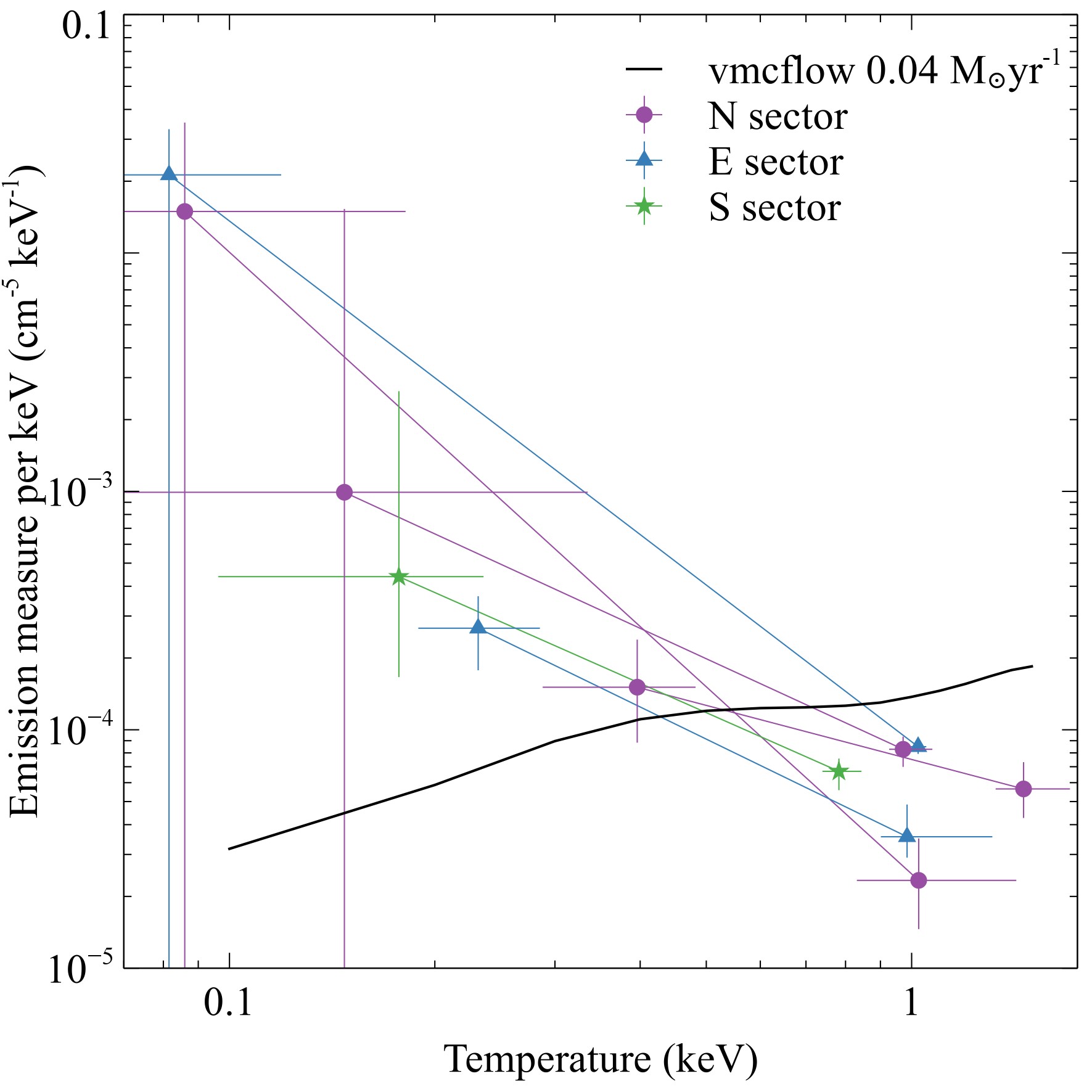
Figure 11: Emission measure per unit energy as a function of temperature for the two component spectral models fit to spectra extracted from within the Bondi radius. The black line shows the expected distribution of emission measure for a $0.04\hbox{$\hbox{$\rm\thinspace M_{\odot}$}\rm\;yr^{-1}\,$}$ cooling flow with the same metallicity structure.

4.2 A settling flow within the Bondi sphere

Assuming a steady-state, spherical flow of gas, we can use the measurements of the gas density and temperature at the Bondi radius to put limits on the radial flow speed and accretion rate. In terms of entropy, $S$, the energy equation for steady spherical flow is

$$\rho Tv_{\mathrm{r}}\left(\frac{\mathrm{d}S}{\mathrm{d}r}\right)=n_{\mathrm{e}}n_{\mathrm{H}}\Lambda,$$ (4)

where $v_{r}$ is the inflow speed, $\rho$ is the gas density, $T$ is the temperature and $n_{\mathrm{e}}n_{\mathrm{H}}\Lambda$ is the energy radiated (see eg. Fabian & Nulsen 1977). Equation 4 can also be written as

$$v_{\mathrm{r}}\left(\frac{\mathrm{d\ln}K}{\mathrm{d\ln}r}\right)=\frac{r}{t_{\mathrm{cool}}},$$ (5)

where $K$ is now entropy as defined in the literature for studies of galaxy clusters $K=k_{\mathrm{B}}T/n_{\mathrm{e}}^{2/3}$ (eg. Voit 2005). Variations in $\mathrm{d\ln}K/\mathrm{d\ln}r$ are assumed to be negligible.

For the N sector, at a radius of $0.12\rm\;kpc$ ($1.5\rm\;arcsec$), the cooling time of the $1\rm\;keV$ gas is $0.014\pm 0.004\rm\;Gyr$ and the corresponding entropy gradient $\mathrm{dln}K/\mathrm{dln}r=1.04\pm 0.09$. The inflow velocity is then $8\pm 2\hbox{$\rm\;km\rm\;s^{-1}\,$}$. Similarly in the S sector the inflow velocity is $9\pm 1\hbox{$\rm\;km\rm\;s^{-1}\,$}$. In practice, this is an upper limit on the flow velocity because the gas may be heated and not flowing inward. If gas was flowing in at a higher velocity than this limit, it would be unable to cool and the entropy gradient should be shallower than observed. The flow velocity within the Bondi sphere is therefore subsonic, which indicates a settling flow rather than a Bondi flow. The gas flow must be supported by pressure or rotation or both. We therefore rule out Bondi accretion on the scale resolved at the Bondi radius.

Mass conservation for the gas flow is given by

$$\dot{m}_{\mathrm{acc}}=4\pi\rho v_{\mathrm{r}}r^{2},$$ (6)

where the gas density $\rho=\mu m_{\mathrm{H}}n$, $\mu m_{\mathrm{H}}$ is the mean gas mass per particle and $n$ is the total particle number density. By substituting for $v_{\mathrm{r}}$ in equation 5 with equation 6, the expected density profile can be expressed as

$$\rho{\propto}r^{-3/2}\left(\frac{\dot{m}_{\mathrm{acc}}T}{\Lambda\left(T\right)}\right)^{1/2}.$$ (7)

The gas temperature profile is roughly isothermal at the Bondi radius and should transition to $T{\propto}r^{-1}$ on smaller scales. For bremsstrahlung cooling, the cooling function $\Lambda{\propto}T^{1/2}$. Therefore, for a steady spherical flow with constant $\dot{m}_{\mathrm{acc}}$, the density profile should steepen from $\rho{\propto}r^{-3/2}$ at the Bondi radius to $\rho{\propto}r^{-7/4}$ at smaller radii where the temperature transitions to $T{\propto}1/r$. The measured density profile slopes to the N and S are consistent with $\rho{\propto}r^{-3/2}$ (section 3.2), as expected for the roughly isothermal temperature profile. The density gradient to the E along the jet axis is significantly shallower at $\rho{\propto}r^{-0.93\pm 0.07}$, which likely indicates an outflow driven by the jet. The assumption of spherical symmetry is clearly violated by the observed density structure within the Bondi radius. Within the Bondi radius, the density gradients are consistent with steady inflow to the N and S, whilst the shallower gradient to the E indicates disruption by the jet activity.

Although equation 6 assumes spherical symmetry, which is violated on the scale of the Bondi radius, it can provide an estimate of the mass inflow rate. In the N sector, the electron density $n_{\mathrm{e}}=0.88\pm 0.15\hbox{$\rm\;cm^{-3}\,$}$ at a radius of $0.12\rm\;kpc$. Therefore, the spherical mass accretion rate $\dot{m}_{\mathrm{acc}}\lesssim 0.010\pm 0.003\hbox{$\hbox{$\rm\thinspace M_{\odot}$}\rm\;yr^{-1}\,$}$. The estimated spherical mass accretion rate limit is consistent in the S sector. We can compare this upper limit on the accretion rate for a steady spherical inflow with the Bondi accretion rate. For the N sector, the Bondi rate in the $1\rm\;keV$ gas is $0.1-0.5\hbox{$\hbox{$\rm\thinspace M_{\odot}$}\rm\;yr^{-1}\,$}$, where the range reflects the uncertainty on the black hole mass (section 3.3). This is a factor of ten higher than our upper limit on the accretion rate. A similar result is obtained for the E and S sectors. This result is consistent with the low inflow velocity, which indicates a much lower accretion rate than the Bondi rate.

From the $PV$ work done by the radio jet to displace the hot gas in the cavities, the mechanical jet power is $8^{+7}_{-3}\times 10^{42}\hbox{$\rm\;erg\rm\;s^{-1}\,$}$ (eg. Reynolds et al. 1996a; Bicknell & Begelman 1999; Di Matteo et al. 2003; Rafferty et al. 2006). The nuclear bolometric luminosity is roughly an order of magnitude lower at $L_{\mathrm{bol}}\sim 2\times 10^{41}\hbox{$\rm\;erg\rm\;s^{-1}\,$}$ (Reynolds et al. 1996b; Di Matteo et al. 2003). Assuming an efficiency of $10\%$, our accretion rate limit of $\lesssim 0.010\pm 0.003\hbox{$\hbox{$\rm\thinspace M_{\odot}$}\rm\;yr^{-1}\,$}$ could supply $P_{\mathrm{acc}}<6\pm 2\times 10^{43}\hbox{$\rm\;erg\rm\;s^{-1}\,$}$. Therefore, the inflow rate appears to supply roughly an order of magnitude more power than is required for the AGN activity.

4.3 Outflow

Numerical simulations of hot accretion flows, such as advection-dominated accretion flows (ADAFs, Ichimaru 1977; Rees et al. 1982; Narayan & Yi 1994), found that outflows are ubiquitous and the inflow rate is expected to decrease with decreasing radius (for a review see Yuan & Narayan 2014). This should flatten the density profile from $\rho{\propto}r^{-1.5}$ expected for a constant inflow rate to $\rho{\propto}r^{-p}$, where $p$ is typically $0.5-1$ (eg. Igumenshchev & Abramowicz 1999; Stone et al. 1999; Stone & Pringle 2001; Hawley & Balbus 2002; Yuan & Bu 2010; Begelman 2012). The majority of the inflowing material is ejected before it reaches the event horizon by winds off the rotationally supported accretion flow. Faraday rotation measurements can probe this region on scales of tens of Schwarzchild radii, $r_{\mathrm{s}}$, and constrain the accretion rate. These results can be compared with X-ray measurements, which are sensitive to the outer radial density profile. Chandra observations combined with Faraday rotation measurements in Sgr A* and NGC 3115 indicate shallow density profiles at the Bondi radius (Wang et al. 2013; Wong et al. 2014) and reduced accretion rates at $r\leq 100r_{\mathrm{s}}$ (Bower et al. 2003; Marrone et al. 2006, 2007; Macquart et al. 2006) with $\lesssim 1\%$ of the matter captured at the Bondi radius reaching the inner regions of the accretion flow. In M87, the measured density profile slopes to the N and S are consistent with $\rho{\propto}r^{-3/2}$ whilst the gradient along the jet axis is significantly flatter with $\rho{\propto}r^{-0.93\pm 0.07}$. This flatter density gradient indicates an outflow directed along the jet axis. Faraday rotation measurements for M87 constrain the accretion rate on scales of $\sim 10r_{\mathrm{s}}$ to be an order of magnitude below our upper limit on the inflow rate at the Bondi radius (Kuo et al. 2014). The majority of the material that is gravitationally captured at the Bondi radius is therefore lost before it reaches the SMBH, either in an outflow or consumed by star formation (section 4.1). We note that this analysis assumes that the observed Faraday rotation originates in the accretion flow and that the density profile follows a powerlaw $n{\propto}r^{-\beta}$ with $\beta\leqslant 3/2$.

4.4 Depletion of metals

The sharp drop in metal abundance within the central few kpc in M87 was first found for Fe and Si abundances in XMM-Newton observations (Böhringer et al. 2001). Although the Chandra observations presented here cannot effectively constrain individual metal abundances, we confirm that the metallicity drops from $2\hbox{$\thinspace\mathrm{Z}_{\odot}$}$ to $0.75\hbox{$\thinspace\mathrm{Z}_{\odot}$}$ within the central $\sim 1.5\rm\;kpc$. This region is strongly multi-phase therefore we employ up to three model temperature components as required and find that the metallicity drop is robust. The hot gas should be strongly enriched by centrally peaked stellar mass loss and supernovae but instead the metallicity drops sharply. Central declines in metallicity have been found in a number of other cool core galaxy clusters (eg. Sanders & Fabian 2002; Johnstone et al. 2002; Panagoulia et al. 2013, 2015). This decline appears to be due to a real absence of iron rather than resonance scattering or a spectral fitting bias.

The hot atmosphere within the central few kpc of M87 has a multiphase structure with gas blobs cooling rapidly down out of the X-ray band and a dusty, filamentary cool gas nebula. The cooler phases must be shielded from the surrounding hot X-ray gas at a few keV (eg. Donahue et al. 2011), presumably by magnetic fields (eg. Fabian et al. 2008). Iron, and other elements such as silicon, may adsorb onto cold dust grains (eg. Draine 2009) and therefore are heavily depleted from the hot gas. Measurements of the dust mass in M87 are complicated by the strong synchrotron emission from the jet (eg. Perlman et al. 2007; Buson et al. 2009; Baes et al. 2010). Recent Herschel observations that cover the far IR indicate a dust mass of $2.2\pm 0.2\times 10^{5}\hbox{$\rm\thinspace M_{\odot}$}$ (di Serego Alighieri et al. 2013), which is consistent with previous upper limits. For Lodders (2003) abundances and an average electron density of $\sim 0.3\hbox{$\rm\;cm^{-3}\,$}$, we estimate that $\sim 10^{5}\hbox{$\rm\thinspace M_{\odot}$}$ of Fe must have been depleted onto dust grains within the central $1.3\rm\;kpc$ to explain the drop in metallicity from $2$ to $0.75\hbox{$\thinspace\mathrm{Z}_{\odot}$}$. Böhringer et al. (2001) found a similar drop in the Si and O abundances. Therefore, the total mass that must have been depleted onto dust is very similar to the total dust mass.

5 Conclusions

Using a new $300\rm\;ks$ short frame time Chandra observation of the centre of M87, we have studied the detailed structure of the hot gas atmosphere within the Bondi radius of the supermassive black hole. We found that:

• The hot gas is multiphase on these scales with temperatures spanning $0.2$ to $1\rm\;keV$. The radiative cooling time of the lowest temperature $0.2\rm\;keV$ gas drops to only $0.1-0.5\rm\;Myr$, which is comparable to the free fall time. The lowest temperature and most rapidly cooling gas in M87 is therefore located at the smallest radii that we can resolve ($\sim 100\rm\;pc$).

• Whilst the temperature structure appears remarkably symmetric about the nucleus inside the Bondi radius, the density gradient is significantly shallower along the jet axis. The density profiles in each sector analysed plateau around the inner cavity structures from $0.5-1\rm\;kpc$ and then smoothly steepen within the Bondi radius to $\sim 1\hbox{$\rm\;cm^{-3}\,$}$ with cooler blobs at $>2\hbox{$\rm\;cm^{-3}\,$}$. The best-fit powerlaw slopes in the N and S sectors, perpendicular to the jet axis, are $-1.4\pm 0.1$ and $-1.6\pm 0.1$, respectively, compared to $-0.93\pm 0.07$ in the E sector along the jet axis. The density structure within the Bondi radius of M87 is therefore consistent with steady inflow perpendicular to the jet axis and outflow directed along the jet axis.

• By putting limits on the radial flow speed $v_{\mathrm{r}}<8\pm 2\hbox{$\rm\;km\rm\;s^{-1}\,$}$, we rule out Bondi accretion on the scale resolved at the Bondi radius. The flow velocity within the Bondi sphere is subsonic, which indicates a settling flow rather than a Bondi flow. The gas flow must be supported by pressure or rotation or both. We estimate the spherical mass inflow rate $\dot{m}_{\mathrm{acc}}\lesssim 0.010\pm 0.003\hbox{$\hbox{$\rm\thinspace M_{\odot}$}\rm\;yr^{-1}\,$}$. Assuming an efficiency of 10%, this inflow rate could supply roughly an order of magnitude more power than is required for the AGN activity. However, much of this material may be lost in an outflow or consumed by star formation before it is accreted by the SMBH.

• The hot gas within the Bondi radius of M87 may form a mini cooling flow. The deprojected spectra extracted within the Bondi radius can be fit equivalently by a two temperature thermal model, with components at $0.2$ and $1\rm\;keV$, or by a single cooling flow model (no additional thermal components) with gas cooling from $1.5\rm\;keV$ to the lower limit of $0.08\rm\;keV$. The best-fit cooling rate of $0.03\hbox{$\hbox{$\rm\thinspace M_{\odot}$}\rm\;yr^{-1}\,$}$ is consistent with the limit on gas cooling below $0.5\rm\;keV$ from the XMM-Newton RGS. HST observations have shown that the circumnuclear gas disk has a radius of $80\rm\;pc$ and therefore lies within a putative transition to a cooling flow at $80-250\rm\;pc$. If the cooling gas has significant angular momentum, it may feed into the circumnuclear gas disk. Based on the upper limits for the cold gas mass in the disk, we estimate that the mini cooling flow could supply sufficient material on timescales of a few $\times 10^{7-8}\rm\;yr$.

• The proposed successor missions to Chandra, including AXIS and Lynx, will resolve these transitions in the hot gas flow within the Bondi radius in many more systems and identify trends with jet power or molecular gas structure. Improved sensitivity at low energies will also be essential to trace this rapidly cooling gas closer to the nucleus.

References

- Arnaud (1996) Arnaud K. A., 1996, in Jacoby G. H., Barnes J., eds, Astronomical Society of the Pacific Conference Series Vol. 101, Astronomical Data Analysis Software and Systems V. pp 17–+
- Baes et al. (2010) Baes M., et al., 2010, \hrefhttp://dx.doi.org/10.1051/0004-6361/201014555 A&A, \hrefhttp://adsabs.harvard.edu/abs/2010A%26A…518L..53B 518, L53
- Baganoff et al. (2003) Baganoff F. K., et al., 2003, \hrefhttp://dx.doi.org/10.1086/375145 ApJ, \hrefhttp://adsabs.harvard.edu/abs/2003ApJ…591..891B 591, 891
- Begelman (2012) Begelman M. C., 2012, \hrefhttp://dx.doi.org/10.1111/j.1365-2966.2011.20071.x MNRAS, \hrefhttp://adsabs.harvard.edu/abs/2012MNRAS.420.2912B 420, 2912
- Bicknell & Begelman (1996) Bicknell G. V., Begelman M. C., 1996, \hrefhttp://dx.doi.org/10.1086/177636 ApJ, \hrefhttp://adsabs.harvard.edu/abs/1996ApJ…467..597B 467, 597
- Bicknell & Begelman (1999) Bicknell G. V., Begelman M. C., 1999, in Röser H.-J., Meisenheimer K., eds, Lecture Notes in Physics, Berlin Springer Verlag Vol. 530, The Radio Galaxy Messier 87. p. 235, \hrefhttp://dx.doi.org/10.1007/BFb0106435 doi:10.1007/BFb0106435
- Bohringer et al. (1995) Bohringer H., Nulsen P. E. J., Braun R., Fabian A. C., 1995, MNRAS, \hrefhttp://adsabs.harvard.edu/abs/1995MNRAS.274L..67B 274, L67
- Böhringer et al. (2001) Böhringer H., et al., 2001, \hrefhttp://dx.doi.org/10.1051/0004-6361:20000092 A&A, \hrefhttp://adsabs.harvard.edu/abs/2001A%26A…365L.181B 365, L181
- Bondi (1952) Bondi H., 1952, MNRAS, \hrefhttp://adsabs.harvard.edu/abs/1952MNRAS.112..195B 112, 195
- Bower et al. (2003) Bower G. C., Wright M. C. H., Falcke H., Backer D. C., 2003, \hrefhttp://dx.doi.org/10.1086/373989 ApJ, \hrefhttp://adsabs.harvard.edu/abs/2003ApJ…588..331B 588, 331
- Bower et al. (2006) Bower R. G., Benson A. J., Malbon R., Helly J. C., Frenk C. S., Baugh C. M., Cole S., Lacey C. G., 2006, \hrefhttp://dx.doi.org/10.1111/j.1365-2966.2006.10519.x MNRAS, \hrefhttp://adsabs.harvard.edu/abs/2006MNRAS.370..645B 370, 645
- Braine & Wiklind (1993) Braine J., Wiklind T., 1993, A&A, \hrefhttp://adsabs.harvard.edu/abs/1993A%26A…267L..47B 267, L47
- Buote (2000) Buote D. A., 2000, \hrefhttp://dx.doi.org/10.1046/j.1365-8711.2000.03046.x MNRAS, \hrefhttp://adsabs.harvard.edu/abs/2000MNRAS.311..176B 311, 176
- Buson et al. (2009) Buson L., et al., 2009, \hrefhttp://dx.doi.org/10.1088/0004-637X/705/1/356 ApJ, \hrefhttp://adsabs.harvard.edu/abs/2009ApJ…705..356B 705, 356
- Carter et al. (2003) Carter C., Karovska M., Jerius D., Glotfelty K., Beikman S., 2003, in Payne H. E., Jedrzejewski R. I., Hook R. N., eds, Astronomical Society of the Pacific Conference Series Vol. 295, Astronomical Data Analysis Software and Systems XII. pp 477–+
- Cash (1979) Cash W., 1979, \hrefhttp://dx.doi.org/10.1086/156922 ApJ, \hrefhttp://adsabs.harvard.edu/abs/1979ApJ…228..939C 228, 939
- Cavagnolo et al. (2009) Cavagnolo K. W., Donahue M., Voit G. M., Sun M., 2009, \hrefhttp://dx.doi.org/10.1088/0067-0049/182/1/12 ApJS, \hrefhttp://adsabs.harvard.edu/abs/2009ApJS..182…12C 182, 12
- Combes et al. (2007) Combes F., Young L. M., Bureau M., 2007, \hrefhttp://dx.doi.org/10.1111/j.1365-2966.2007.11759.x MNRAS, \hrefhttp://adsabs.harvard.edu/abs/2007MNRAS.377.1795C 377, 1795
- Croton et al. (2006) Croton D. J., et al., 2006, \hrefhttp://dx.doi.org/10.1111/j.1365-2966.2005.09675.x MNRAS, \hrefhttp://adsabs.harvard.edu/abs/2006MNRAS.365…11C 365, 11
- Davis (2001) Davis J. E., 2001, \hrefhttp://dx.doi.org/10.1086/323488 ApJ, \hrefhttp://adsabs.harvard.edu/abs/2001ApJ…562..575D 562, 575
- Davis et al. (2012) Davis J. E., et al., 2012, in Space Telescopes and Instrumentation 2012: Ultraviolet to Gamma Ray. p. 84431A, \hrefhttp://dx.doi.org/10.1117/12.926937 doi:10.1117/12.926937
- Di Matteo et al. (2003) Di Matteo T., Allen S. W., Fabian A. C., Wilson A. S., Young A. J., 2003, \hrefhttp://dx.doi.org/10.1086/344504 ApJ, \hrefhttp://adsabs.harvard.edu/abs/2003ApJ…582..133D 582, 133
- Donahue et al. (2011) Donahue M., de Messières G. E., O’Connell R. W., Voit G. M., Hoffer A., McNamara B. R., Nulsen P. E. J., 2011, \hrefhttp://dx.doi.org/10.1088/0004-637X/732/1/40 ApJ, \hrefhttp://adsabs.harvard.edu/abs/2011ApJ…732…40D 732, 40
- Draine (2009) Draine B. T., 2009, in Henning T., Grün E., Steinacker J., eds, Astronomical Society of the Pacific Conference Series Vol. 414, Cosmic Dust - Near and Far. p. 453 (\hrefhttp://arxiv.org/abs/0903.1658 arXiv:0903.1658)
- Fabian (2012) Fabian A. C., 2012, \hrefhttp://dx.doi.org/10.1146/annurev-astro-081811-125521 ARA&A, \hrefhttp://adsabs.harvard.edu/abs/2012ARA%26A..50..455F 50, 455
- Fabian & Nulsen (1977) Fabian A. C., Nulsen P. E. J., 1977, \hrefhttp://dx.doi.org/10.1093/mnras/180.3.479 MNRAS, \hrefhttp://adsabs.harvard.edu/abs/1977MNRAS.180..479F 180, 479
- Fabian et al. (2008) Fabian A. C., Johnstone R. M., Sanders J. S., Conselice C. J., Crawford C. S., Gallagher III J. S., Zweibel E., 2008, \hrefhttp://dx.doi.org/10.1038/nature07169 Nat, \hrefhttp://adsabs.harvard.edu/abs/2008Natur.454..968F 454, 968
- Ford et al. (1994) Ford H. C., et al., 1994, \hrefhttp://dx.doi.org/10.1086/187586 ApJ, \hrefhttp://adsabs.harvard.edu/abs/1994ApJ…435L..27F 435, L27
- Forman et al. (2005) Forman W., et al., 2005, \hrefhttp://dx.doi.org/10.1086/429746 ApJ, \hrefhttp://adsabs.harvard.edu/abs/2005ApJ…635..894F 635, 894
- Forman et al. (2007) Forman W., et al., 2007, \hrefhttp://dx.doi.org/10.1086/519480 ApJ, \hrefhttp://adsabs.harvard.edu/abs/2007ApJ…665.1057F 665, 1057
- Forman et al. (2017) Forman W., Churazov E., Jones C., Heinz S., Kraft R., Vikhlinin A., 2017, \hrefhttp://dx.doi.org/10.3847/1538-4357/aa70e4 ApJ, \hrefhttp://adsabs.harvard.edu/abs/2017ApJ…844..122F 844, 122
- Fruscione et al. (2006) Fruscione A., et al., 2006, in Society of Photo-Optical Instrumentation Engineers (SPIE) Conference Series. , \hrefhttp://dx.doi.org/10.1117/12.671760 doi:10.1117/12.671760
- Gaspari et al. (2013) Gaspari M., Ruszkowski M., Oh S. P., 2013, \hrefhttp://dx.doi.org/10.1093/mnras/stt692 MNRAS, \hrefhttp://adsabs.harvard.edu/abs/2013MNRAS.432.3401G 432, 3401
- Gebhardt & Thomas (2009) Gebhardt K., Thomas J., 2009, \hrefhttp://dx.doi.org/10.1088/0004-637X/700/2/1690 ApJ, \hrefhttp://adsabs.harvard.edu/abs/2009ApJ…700.1690G 700, 1690
- Gebhardt et al. (2011) Gebhardt K., Adams J., Richstone D., Lauer T. R., Faber S. M., Gültekin K., Murphy J., Tremaine S., 2011, \hrefhttp://dx.doi.org/10.1088/0004-637X/729/2/119 ApJ, \hrefhttp://adsabs.harvard.edu/abs/2011ApJ…729..119G 729, 119
- Harms et al. (1994) Harms R. J., et al., 1994, \hrefhttp://dx.doi.org/10.1086/187588 ApJ, \hrefhttp://adsabs.harvard.edu/abs/1994ApJ…435L..35H 435, L35
- Harris et al. (2006) Harris D. E., Cheung C. C., Biretta J. A., Sparks W. B., Junor W., Perlman E. S., Wilson A. S., 2006, \hrefhttp://dx.doi.org/10.1086/500081 ApJ, \hrefhttp://adsabs.harvard.edu/abs/2006ApJ…640..211H 640, 211
- Harris et al. (2009) Harris D. E., Cheung C. C., Stawarz Ł., Biretta J. A., Perlman E. S., 2009, \hrefhttp://dx.doi.org/10.1088/0004-637X/699/1/305 ApJ, \hrefhttp://adsabs.harvard.edu/abs/2009ApJ…699..305H 699, 305
- Harris et al. (2011) Harris D. E., et al., 2011, \hrefhttp://dx.doi.org/10.1088/0004-637X/743/2/177 ApJ, \hrefhttp://adsabs.harvard.edu/abs/2011ApJ…743..177H 743, 177
- Hawley & Balbus (2002) Hawley J. F., Balbus S. A., 2002, \hrefhttp://dx.doi.org/10.1086/340765 ApJ, \hrefhttp://adsabs.harvard.edu/abs/2002ApJ…573..738H 573, 738
- Ho (2008) Ho L. C., 2008, \hrefhttp://dx.doi.org/10.1146/annurev.astro.45.051806.110546 ARA&A, \hrefhttp://adsabs.harvard.edu/abs/2008ARA%26A..46..475H 46, 475
- Ho (2009) Ho L. C., 2009, \hrefhttp://dx.doi.org/10.1088/0004-637X/699/1/626 ApJ, \hrefhttp://adsabs.harvard.edu/abs/2009ApJ…699..626H 699, 626
- Hopkins et al. (2006) Hopkins P. F., Hernquist L., Cox T. J., Di Matteo T., Robertson B., Springel V., 2006, \hrefhttp://dx.doi.org/10.1086/499298 ApJS, \hrefhttp://adsabs.harvard.edu/abs/2006ApJS..163….1H 163, 1
- Ichimaru (1977) Ichimaru S., 1977, \hrefhttp://dx.doi.org/10.1086/155314 ApJ, \hrefhttp://adsabs.harvard.edu/abs/1977ApJ…214..840I 214, 840
- Igumenshchev & Abramowicz (1999) Igumenshchev I. V., Abramowicz M. A., 1999, \hrefhttp://dx.doi.org/10.1046/j.1365-8711.1999.02220.x MNRAS, \hrefhttp://adsabs.harvard.edu/abs/1999MNRAS.303..309I 303, 309
- Jerius (2002) Jerius D., 2002, Comparison of on-axis Chandra Observations of AR Lac to SAOsac Simulations
- Jerius et al. (1995) Jerius D., Freeman M., Gaetz T., Hughes J. P., Podgorski W., 1995, in Shaw R. A., Payne H. E., Hayes J. J. E., eds, Astronomical Society of the Pacific Conference Series Vol. 77, Astronomical Data Analysis Software and Systems IV. pp 357–+
- Jerius et al. (2000) Jerius D., Donnelly R. H., Tibbetts M. S., Edgar R. J., Gaetz T. J., Schwartz D. A., Van Speybroeck L. P., Zhao P., 2000, in Truemper J. E., Aschenbach B., eds, Proc. SPIE Vol. 4012, X-Ray Optics, Instruments, and Missions III. pp 17–27, \hrefhttp://dx.doi.org/10.1117/12.391555 doi:10.1117/12.391555
- Johnstone et al. (1992) Johnstone R. M., Fabian A. C., Edge A. C., Thomas P. A., 1992, \hrefhttp://dx.doi.org/10.1093/mnras/255.3.431 MNRAS, \hrefhttp://adsabs.harvard.edu/abs/1992MNRAS.255..431J 255, 431
- Johnstone et al. (2002) Johnstone R. M., Allen S. W., Fabian A. C., Sanders J. S., 2002, \hrefhttp://dx.doi.org/10.1046/j.1365-8711.2002.05743.x MNRAS, \hrefhttp://adsabs.harvard.edu/abs/2002MNRAS.336..299J 336, 299
- Kalberla et al. (2005) Kalberla P. M. W., Burton W. B., Hartmann D., Arnal E. M., Bajaja E., Morras R., Pöppel W. G. L., 2005, \hrefhttp://dx.doi.org/10.1051/0004-6361:20041864 A&A, \hrefhttp://adsabs.harvard.edu/abs/2005A%26A…440..775K 440, 775
- Kuo et al. (2014) Kuo C. Y., et al., 2014, \hrefhttp://dx.doi.org/10.1088/2041-8205/783/2/L33 ApJ, \hrefhttp://adsabs.harvard.edu/abs/2014ApJ…783L..33K 783, L33
- Li et al. (2004) Li J., Kastner J. H., Prigozhin G. Y., Schulz N. S., Feigelson E. D., Getman K. V., 2004, \hrefhttp://dx.doi.org/10.1086/421866 ApJ, \hrefhttp://adsabs.harvard.edu/abs/2004ApJ…610.1204L 610, 1204
- Li et al. (2013) Li J., Ostriker J., Sunyaev R., 2013, \hrefhttp://dx.doi.org/10.1088/0004-637X/767/2/105 ApJ, \hrefhttp://adsabs.harvard.edu/abs/2013ApJ…767..105L 767, 105
- Lieu et al. (1996) Lieu R., Mittaz J. P. D., Bowyer S., Lockman F. J., Hwang C.-Y., Schmitt J. H. M. M., 1996, \hrefhttp://dx.doi.org/10.1086/309908 ApJ, \hrefhttp://adsabs.harvard.edu/abs/1996ApJ…458L…5L 458, L5
- Lodders (2003) Lodders K., 2003, \hrefhttp://dx.doi.org/10.1086/375492 ApJ, \hrefhttp://adsabs.harvard.edu/abs/2003ApJ…591.1220L 591, 1220
- Macchetto et al. (1997) Macchetto F., Marconi A., Axon D. J., Capetti A., Sparks W., Crane P., 1997, \hrefhttp://dx.doi.org/10.1086/304823 ApJ, \hrefhttp://adsabs.harvard.edu/abs/1997ApJ…489..579M 489, 579
- Macquart et al. (2006) Macquart J.-P., Bower G. C., Wright M. C. H., Backer D. C., Falcke H., 2006, \hrefhttp://dx.doi.org/10.1086/506932 ApJ, \hrefhttp://adsabs.harvard.edu/abs/2006ApJ…646L.111M 646, L111
- Marrone et al. (2006) Marrone D. P., Moran J. M., Zhao J.-H., Rao R., 2006, \hrefhttp://dx.doi.org/10.1086/500106 ApJ, \hrefhttp://adsabs.harvard.edu/abs/2006ApJ…640..308M 640, 308
- Marrone et al. (2007) Marrone D. P., Moran J. M., Zhao J.-H., Rao R., 2007, \hrefhttp://dx.doi.org/10.1086/510850 ApJ, \hrefhttp://adsabs.harvard.edu/abs/2007ApJ…654L..57M 654, L57
- Mathews et al. (2001) Mathews W. G., Buote D. A., Brighenti F., 2001, \hrefhttp://dx.doi.org/10.1086/319497 ApJ, \hrefhttp://adsabs.harvard.edu/abs/2001ApJ…550L..31M 550, L31
- McKinney et al. (2012) McKinney J. C., Tchekhovskoy A., Blandford R. D., 2012, \hrefhttp://dx.doi.org/10.1111/j.1365-2966.2012.21074.x MNRAS, \hrefhttp://adsabs.harvard.edu/abs/2012MNRAS.423.3083M 423, 3083
- McNamara & Nulsen (2007) McNamara B. R., Nulsen P. E. J., 2007, \hrefhttp://dx.doi.org/10.1146/annurev.astro.45.051806.110625 ARA&A, \hrefhttp://adsabs.harvard.edu/abs/2007ARA%26A..45..117M 45, 117
- McNamara & O’Connell (1989) McNamara B. R., O’Connell R. W., 1989, \hrefhttp://dx.doi.org/10.1086/115275 AJ, \hrefhttp://adsabs.harvard.edu/abs/1989AJ…..98.2018M 98, 2018
- McNamara et al. (2011) McNamara B. R., Rohanizadegan M., Nulsen P. E. J., 2011, \hrefhttp://dx.doi.org/10.1088/0004-637X/727/1/39 ApJ, \hrefhttp://adsabs.harvard.edu/abs/2011ApJ…727…39M 727, 39
- Miller et al. (2017) Miller J. M., Bautz M. W., McNamara B. R., 2017, \hrefhttp://dx.doi.org/10.3847/2041-8213/aa9566 ApJ, \hrefhttp://adsabs.harvard.edu/abs/2017ApJ…850L…3M 850, L3
- Million et al. (2010) Million E. T., Werner N., Simionescu A., Allen S. W., Nulsen P. E. J., Fabian A. C., Böhringer H., Sanders J. S., 2010, \hrefhttp://dx.doi.org/10.1111/j.1365-2966.2010.17220.x MNRAS, \hrefhttp://adsabs.harvard.edu/abs/2010MNRAS.407.2046M 407, 2046
- Million et al. (2011) Million E. T., Werner N., Simionescu A., Allen S. W., 2011, \hrefhttp://dx.doi.org/10.1111/j.1365-2966.2011.19664.x MNRAS, \hrefhttp://adsabs.harvard.edu/abs/2011MNRAS.418.2744M 418, 2744
- Mushotzky & Szymkowiak (1988) Mushotzky R. F., Szymkowiak A. E., 1988, in Fabian A. C., ed., NATO Advanced Science Institutes (ASI) Series C Vol. 229, NATO Advanced Science Institutes (ASI) Series C. pp 53–62
- Narayan & McClintock (2008) Narayan R., McClintock J. E., 2008, \hrefhttp://dx.doi.org/10.1016/j.newar.2008.03.002 NewA Rev., \hrefhttp://adsabs.harvard.edu/abs/2008NewAR..51..733N 51, 733
- Narayan & Yi (1994) Narayan R., Yi I., 1994, \hrefhttp://dx.doi.org/10.1086/187381 ApJ, \hrefhttp://adsabs.harvard.edu/abs/1994ApJ…428L..13N 428, L13
- Nemmen & Tchekhovskoy (2015) Nemmen R. S., Tchekhovskoy A., 2015, \hrefhttp://dx.doi.org/10.1093/mnras/stv260 MNRAS, \hrefhttp://adsabs.harvard.edu/abs/2015MNRAS.449..316N 449, 316
- Ocaña Flaquer et al. (2010) Ocaña Flaquer B., Leon S., Combes F., Lim J., 2010, \hrefhttp://dx.doi.org/10.1051/0004-6361/200913392 A&A, \hrefhttp://adsabs.harvard.edu/abs/2010A%26A…518A…9O 518, A9
- Oldham & Auger (2016) Oldham L. J., Auger M. W., 2016, \hrefhttp://dx.doi.org/10.1093/mnras/stv2982 MNRAS, \hrefhttp://adsabs.harvard.edu/abs/2016MNRAS.457..421O 457, 421
- Panagoulia et al. (2013) Panagoulia E. K., Fabian A. C., Sanders J. S., 2013, \hrefhttp://dx.doi.org/10.1093/mnras/stt969 MNRAS, \hrefhttp://adsabs.harvard.edu/abs/2013MNRAS.433.3290P 433, 3290
- Panagoulia et al. (2015) Panagoulia E. K., Sanders J. S., Fabian A. C., 2015, \hrefhttp://dx.doi.org/10.1093/mnras/stu2469 MNRAS, \hrefhttp://adsabs.harvard.edu/abs/2015MNRAS.447..417P 447, 417
- Perlman et al. (2007) Perlman E. S., et al., 2007, \hrefhttp://dx.doi.org/10.1086/518781 ApJ, \hrefhttp://adsabs.harvard.edu/abs/2007ApJ…663..808P 663, 808
- Peterson & Fabian (2006) Peterson J. R., Fabian A. C., 2006, \hrefhttp://dx.doi.org/10.1016/j.physrep.2005.12.007 Phys. Rep., \hrefhttp://adsabs.harvard.edu/abs/2006PhR…427….1P 427, 1
- Peterson et al. (2003) Peterson J. R., Kahn S. M., Paerels F. B. S., Kaastra J. S., Tamura T., Bleeker J. A. M., Ferrigno C., Jernigan J. G., 2003, \hrefhttp://dx.doi.org/10.1086/374830 ApJ, \hrefhttp://adsabs.harvard.edu/abs/2003ApJ…590..207P 590, 207
- Pizzolato & Soker (2005) Pizzolato F., Soker N., 2005, \hrefhttp://dx.doi.org/10.1086/444344 ApJ, \hrefhttp://adsabs.harvard.edu/abs/2005ApJ…632..821P 632, 821
- Rafferty et al. (2006) Rafferty D. A., McNamara B. R., Nulsen P. E. J., Wise M. W., 2006, \hrefhttp://dx.doi.org/10.1086/507672 ApJ, \hrefhttp://adsabs.harvard.edu/abs/2006ApJ…652..216R 652, 216
- Rees et al. (1982) Rees M. J., Begelman M. C., Blandford R. D., Phinney E. S., 1982, \hrefhttp://dx.doi.org/10.1038/295017a0 Nat, \hrefhttp://adsabs.harvard.edu/abs/1982Natur.295…17R 295, 17
- Reynolds et al. (1996a) Reynolds C. S., Fabian A. C., Celotti A., Rees M. J., 1996a, \hrefhttp://dx.doi.org/10.1093/mnras/283.3.873 MNRAS, \hrefhttp://adsabs.harvard.edu/abs/1996MNRAS.283..873R 283, 873
- Reynolds et al. (1996b) Reynolds C. S., Di Matteo T., Fabian A. C., Hwang U., Canizares C. R., 1996b, MNRAS, \hrefhttp://adsabs.harvard.edu/abs/1996MNRAS.283L.111R 283, L111
- Russell et al. (2008) Russell H. R., Sanders J. S., Fabian A. C., 2008, \hrefhttp://dx.doi.org/10.1111/j.1365-2966.2008.13823.x MNRAS, \hrefhttp://adsabs.harvard.edu/abs/2008MNRAS.390.1207R 390, 1207
- Russell et al. (2010) Russell H. R., Fabian A. C., Sanders J. S., Johnstone R. M., Blundell K. M., Brandt W. N., Crawford C. S., 2010, \hrefhttp://dx.doi.org/10.1111/j.1365-2966.2009.16027.x MNRAS, \hrefhttp://adsabs.harvard.edu/abs/2010MNRAS.402.1561R 402, 1561
- Russell et al. (2013) Russell H. R., McNamara B. R., Edge A. C., Hogan M. T., Main R. A., Vantyghem A. N., 2013, \hrefhttp://dx.doi.org/10.1093/mnras/stt490 MNRAS, \hrefhttp://adsabs.harvard.edu/abs/2013MNRAS.432..530R 432, 530
- Russell et al. (2015) Russell H. R., Fabian A. C., McNamara B. R., Broderick A. E., 2015, \hrefhttp://dx.doi.org/10.1093/mnras/stv954 MNRAS, \hrefhttp://adsabs.harvard.edu/abs/2015MNRAS.451..588R 451, 588
- Sakelliou et al. (2002) Sakelliou I., et al., 2002, \hrefhttp://dx.doi.org/10.1051/0004-6361:20020900 A&A, \hrefhttp://adsabs.harvard.edu/abs/2002A%26A…391..903S 391, 903
- Salomé & Combes (2008) Salomé P., Combes F., 2008, \hrefhttp://dx.doi.org/10.1051/0004-6361:200810262 A&A, \hrefhttp://adsabs.harvard.edu/abs/2008A%26A…489..101S 489, 101
- Sanders & Fabian (2002) Sanders J. S., Fabian A. C., 2002, \hrefhttp://dx.doi.org/10.1046/j.1365-8711.2002.05211.x MNRAS, \hrefhttp://adsabs.harvard.edu/abs/2002MNRAS.331..273S 331, 273
- Sanders & Fabian (2006) Sanders J. S., Fabian A. C., 2006, \hrefhttp://dx.doi.org/10.1111/j.1365-2966.2006.10497.x MNRAS, \hrefhttp://adsabs.harvard.edu/abs/2006MNRAS.370…63S 370, 63
- Sanders & Fabian (2007) Sanders J. S., Fabian A. C., 2007, \hrefhttp://dx.doi.org/10.1111/j.1365-2966.2007.12347.x MNRAS, \hrefhttp://adsabs.harvard.edu/abs/2007MNRAS.381.1381S 381, 1381
- Sanders et al. (2010) Sanders J. S., Fabian A. C., Frank K. A., Peterson J. R., Russell H. R., 2010, \hrefhttp://dx.doi.org/10.1111/j.1365-2966.2009.15902.x MNRAS, \hrefhttp://adsabs.harvard.edu/abs/2010MNRAS.402..127S 402, 127
- Sargent et al. (1978) Sargent W. L. W., Young P. J., Lynds C. R., Boksenberg A., Shortridge K., Hartwick F. D. A., 1978, \hrefhttp://dx.doi.org/10.1086/156077 ApJ, \hrefhttp://adsabs.harvard.edu/abs/1978ApJ…221..731S 221, 731
- Siemiginowska et al. (2010) Siemiginowska A., Burke D. J., Aldcroft T. L., Worrall D. M., Allen S., Bechtold J., Clarke T., Cheung C. C., 2010, \hrefhttp://dx.doi.org/10.1088/0004-637X/722/1/102 ApJ, \hrefhttp://adsabs.harvard.edu/abs/2010ApJ…722..102S 722, 102
- Smith et al. (2001) Smith R. K., Brickhouse N. S., Liedahl D. A., Raymond J. C., 2001, \hrefhttp://dx.doi.org/10.1086/322992 ApJ, \hrefhttp://adsabs.harvard.edu/abs/2001ApJ…556L..91S 556, L91
- Sparks et al. (1993) Sparks W. B., Ford H. C., Kinney A. L., 1993, \hrefhttp://dx.doi.org/10.1086/173022 ApJ, \hrefhttp://adsabs.harvard.edu/abs/1993ApJ…413..531S 413, 531
- Sparks et al. (2004) Sparks W. B., Donahue M., Jordán A., Ferrarese L., Côté P., 2004, \hrefhttp://dx.doi.org/10.1086/383189 ApJ, \hrefhttp://adsabs.harvard.edu/abs/2004ApJ…607..294S 607, 294
- Stone & Pringle (2001) Stone J. M., Pringle J. E., 2001, \hrefhttp://dx.doi.org/10.1046/j.1365-8711.2001.04138.x MNRAS, \hrefhttp://adsabs.harvard.edu/abs/2001MNRAS.322..461S 322, 461
- Stone et al. (1999) Stone J. M., Pringle J. E., Begelman M. C., 1999, \hrefhttp://dx.doi.org/10.1046/j.1365-8711.1999.03024.x MNRAS, \hrefhttp://adsabs.harvard.edu/abs/1999MNRAS.310.1002S 310, 1002
- Tan et al. (2008) Tan J. C., Beuther H., Walter F., Blackman E. G., 2008, \hrefhttp://dx.doi.org/10.1086/592592 ApJ, \hrefhttp://adsabs.harvard.edu/abs/2008ApJ…689..775T 689, 775
- Tchekhovskoy & McKinney (2012) Tchekhovskoy A., McKinney J. C., 2012, \hrefhttp://dx.doi.org/10.1111/j.1745-3933.2012.01256.x MNRAS, \hrefhttp://adsabs.harvard.edu/abs/2012MNRAS.423L..55T 423, L55
- Tchekhovskoy et al. (2011) Tchekhovskoy A., Narayan R., McKinney J. C., 2011, \hrefhttp://dx.doi.org/10.1111/j.1745-3933.2011.01147.x MNRAS, \hrefhttp://adsabs.harvard.edu/abs/2011MNRAS.418L..79T 418, L79
- Tonry et al. (2001) Tonry J. L., Dressler A., Blakeslee J. P., Ajhar E. A., Fletcher A. B., Luppino G. A., Metzger M. R., Moore C. B., 2001, \hrefhttp://dx.doi.org/10.1086/318301 ApJ, \hrefhttp://adsabs.harvard.edu/abs/2001ApJ…546..681T 546, 681
- Tsunemi et al. (2001) Tsunemi H., Mori K., Miyata E., Baluta C., Burrows D. N., Garmire G. P., Chartas G., 2001, \hrefhttp://dx.doi.org/10.1086/321338 ApJ, \hrefhttp://adsabs.harvard.edu/abs/2001ApJ…554..496T 554, 496
- Voit (2005) Voit G. M., 2005, \hrefhttp://dx.doi.org/10.1103/RevModPhys.77.207 Reviews of Modern Physics, \hrefhttp://adsabs.harvard.edu/abs/2005RvMP…77..207V 77, 207
- Wachter et al. (1979) Wachter K., Leach R., Kellogg E., 1979, \hrefhttp://dx.doi.org/10.1086/157084 ApJ, \hrefhttp://adsabs.harvard.edu/abs/1979ApJ…230..274W 230, 274
- Walsh et al. (2013) Walsh J. L., Barth A. J., Ho L. C., Sarzi M., 2013, \hrefhttp://dx.doi.org/10.1088/0004-637X/770/2/86 ApJ, \hrefhttp://adsabs.harvard.edu/abs/2013ApJ…770…86W 770, 86
- Wang et al. (2013) Wang Q. D., et al., 2013, \hrefhttp://dx.doi.org/10.1126/science.1240755 Science, \hrefhttp://adsabs.harvard.edu/abs/2013Sci…341..981W 341, 981
- Werner et al. (2006) Werner N., Böhringer H., Kaastra J. S., de Plaa J., Simionescu A., Vink J., 2006, \hrefhttp://dx.doi.org/10.1051/0004-6361:20065678 A&A, \hrefhttp://adsabs.harvard.edu/abs/2006A%26A…459..353W 459, 353
- Werner et al. (2010) Werner N., et al., 2010, \hrefhttp://dx.doi.org/10.1111/j.1365-2966.2010.16755.x MNRAS, \hrefhttp://adsabs.harvard.edu/abs/2010MNRAS.407.2063W 407, 2063
- Wong et al. (2011) Wong K.-W., Irwin J. A., Yukita M., Million E. T., Mathews W. G., Bregman J. N., 2011, \hrefhttp://dx.doi.org/10.1088/2041-8205/736/1/L23 ApJ, \hrefhttp://adsabs.harvard.edu/abs/2011ApJ…736L..23W 736, L23
- Wong et al. (2014) Wong K.-W., Irwin J. A., Shcherbakov R. V., Yukita M., Million E. T., Bregman J. N., 2014, \hrefhttp://dx.doi.org/10.1088/0004-637X/780/1/9 ApJ, \hrefhttp://adsabs.harvard.edu/abs/2014ApJ…780….9W 780, 9
- Young et al. (2002) Young A. J., Wilson A. S., Mundell C. G., 2002, \hrefhttp://dx.doi.org/10.1086/342918 ApJ, \hrefhttp://adsabs.harvard.edu/abs/2002ApJ…579..560Y 579, 560
- Yuan & Bu (2010) Yuan F., Bu D.-F., 2010, \hrefhttp://dx.doi.org/10.1111/j.1365-2966.2010.17175.x MNRAS, \hrefhttp://adsabs.harvard.edu/abs/2010MNRAS.408.1051Y 408, 1051
- Yuan & Narayan (2014) Yuan F., Narayan R., 2014, \hrefhttp://dx.doi.org/10.1146/annurev-astro-082812-141003 ARA&A, \hrefhttp://adsabs.harvard.edu/abs/2014ARA%26A..52..529Y 52, 529
- Yuan et al. (2012) Yuan F., Wu M., Bu D., 2012, \hrefhttp://dx.doi.org/10.1088/0004-637X/761/2/129 ApJ, \hrefhttp://adsabs.harvard.edu/abs/2012ApJ…761..129Y 761, 129
- di Serego Alighieri et al. (2013) di Serego Alighieri S., et al., 2013, \hrefhttp://dx.doi.org/10.1051/0004-6361/201220551 A&A, \hrefhttp://adsabs.harvard.edu/abs/2013A%26A…552A…8D 552, A8