Comparison of local density functionals based on electron gas and finite systems

Abstract

A widely used approximation to the exchange-correlation functional in density functional theory is the local density approximation (LDA), typically derived from the properties of the homogeneous electron gas (HEG). We previously introduced a set of alternative LDAs constructed from one-dimensional systems of one, two, and three electrons that resemble the HEG within a finite region. We now construct a HEG-based LDA appropriate for spinless electrons in one dimension and find that it is remarkably similar to the finite LDAs. As expected, all LDAs are inadequate in low-density systems where correlation is strong. However, exploring the small but significant differences between the functionals, we find that the finite LDAs give better densities and energies in high-density exchange-dominated systems, arising partly from a better description of the self-interaction correction.

I Introduction

Density functional theory Hohenberg and Kohn (1964) (DFT) is the most popular method to calculate the ground-state properties of many-electron systems Dreizler and Gross (2012); Parr and Yang (1994); Fiolhais et al. (2003); Burke (2012); Martin (2004); Engel and Dreizler (2011). In the widely employed Kohn-Sham Kohn and Sham (1965) (KS) formalism of DFT, the real system of interacting electrons is mapped onto a fictitious system of noninteracting electrons moving in an effective local potential, with both systems having the same electron density. While in principle an exact theory, in practice the accuracy of DFT calculations is constrained by our ability to approximate the exchange-correlation (xc) part of the KS functional, whose exact form is unknown. Identifying properties of the exact xc functional that are missing in commonly used approximations is vital for further developments.

A widely used approximation is the local density approximation Kohn and Sham (1965) (LDA) which assumes that the true xc functional is solely dependent on the electron density at each point in the system. LDAs are traditionally derived from knowledge of the xc energy of the homogeneous electron gas Ceperley and Alder (1980) (HEG), a model system where the exchange energy is known analytically and the correlation energy is usually calculated using quantum Monte Carlo simulations. LDAs have been hugely successful in many cases Dreizler and Gross (2012); Parr and Yang (1994), however, their validity breaks down in a number of important situations Onida et al. (2002); Lein et al. (2000); Gritsenko et al. (2000); Maitra et al. (2002); Burke et al. (2005); Varsano et al. (2008); Jones and Gunnarsson (1989); Pickett (1989); Gonze et al. (1997), particularly when there is strong correlation. They are known to miss out some critical features that are present in the exact xc potential, such as the cancellation of the spurious electron self-interaction Perdew and Zunger (1981); Tozer and Handy (1998); Dreuw et al. (2003), or the Coulomb-type $-1/r$ decay of the xc potential far from a finite system Levy et al. (1984); Almbladh and von Barth (1985), instead following an incorrect exponential decay Perdew and Zunger (1981); Almbladh and von Barth (1985). They also fail to capture the derivative discontinuity Mori-Sanchez and Cohen (2014); Mosquera and Wasserman (2014a, b), the discontinuous nature of the derivative of the xc energy with respect to electron number $N$, at integer $N$.

In a previous paper Entwistle et al. (2016), we introduced a set of LDAs which, in contrast to the traditional HEG LDA, were constructed from systems of one, two, and three electrons which resembled the HEG within a finite region. Illustrating our approach in one dimension (1D), we found that the three LDAs were remarkably similar to one another. In this paper, we construct a 1D HEG LDA through suitable diffusion Monte Carlo Casula et al. (2005) (DMC) techniques, along with a revised set of LDAs constructed from finite systems. We compare the finite and HEG LDAs with one another to demonstrate that local approximations constructed from finite systems are a viable alternative, and explore the nature of any differences between them.

In order to test the LDAs, we employ our iDEA code Hodgson et al. (2013) which solves the many-electron Schrödinger equation exactly for model finite systems to determine the exact, fully-correlated, many-electron wave function. Using this to obtain the exact electron density, we then utilize our reverse engineering algorithm to find the exact KS system. In our calculations we use spinless electrons to more closely approach the nature of exchange and correlation in many-electron systems, which interact via the appropriately softened Coulomb repulsion Gordon et al. (2005)^, $(|x-x^{\prime}|+1)^{-1}$.

II Set of LDAs

II.1 LDAs from finite systems

In Ref. Entwistle et al., 2016 we chose a set of finite locally homogeneous systems in order to mimic the HEG, which we referred to as “slabs” (Fig. 1). We generated sets of one-electron ($1e$), two-electron ($2e$), and three-electron ($3e$) slab systems over a typical density range (up to 0.6 a.u.) and in each case calculated the exact xc energy $E_{\mathrm{xc}}$. From this we parametrized the xc energy density $\varepsilon_{\mathrm{xc}}=E_{\mathrm{xc}}/N$ in terms of the electron density of the plateau region of the slabs, repeating for the $1e$, $2e$, and $3e$ set.

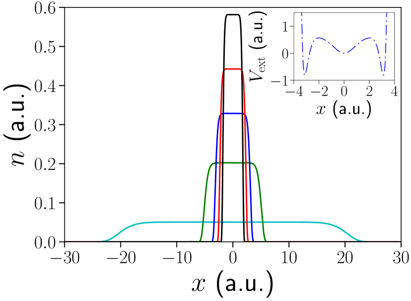
Figure 1: The exact many-body electron density (solid lines) for a selection of the two-electron slab systems. The density is locally homogeneous across a plateau region and decays exponentially at the edges. Inset: the external potential for a typical two-electron slab system (middle density in main figure).

To approximate the xc energy of an inhomogeneous system, the LDA focuses on the local electron density at each point in the system:

$$E_{\mathrm{xc}}^{\mathrm{LDA}}[n]=\int n(x)\varepsilon_{\mathrm{xc}}(n)\ dx,$$ (1)

where in a conventional LDA $\varepsilon_{\mathrm{xc}}(n)$ is the xc energy density of a HEG of density $n$. This approximation becomes exact in the limit of the HEG, and so it is a reasonable requirement for the finite LDAs to become exact in the limit of the slab systems. Due to the initial parametrization of $\varepsilon_{\mathrm{xc}}(n)$ focusing on the plateau regions of the slabs (i.e., ignoring the inhomogeneous regions at the edges), we used a refinement process Entwistle et al. (2016) in order to fulfill this requirement.

The refined form for the xc energy density in the three finite LDAs has now been increased from the four-parameter fit in Ref. Entwistle et al., 2016 to a seven-parameter fit in this paper:

$$\varepsilon_{\mathrm{xc}}(n)=(A+Bn+Cn^{2}+Dn^{3}+En^{4}+Fn^{5})n^{G},$$ (2)

where the optimal parameters for each LDA are given in Table 1. The xc potential $V_{\mathrm{xc}}$ is defined as the functional derivative of the xc energy which in the LDA reduces to a simple form :

$$V_{\mathrm{xc}}^{\mathrm{LDA}}(n)=\varepsilon_{\mathrm{xc}}(n(x))+n(x)\frac{d\varepsilon_{\mathrm{xc}}}{dn}\bigg{|}_{n(x)}.$$ (3)

Table 1: Optimal fit parameters for $\varepsilon_{\mathrm{xc}}(n)$ in the finite LDAs. The last two rows contain the mean absolute error (MAE) and root-mean-square error (RMSE) of the fits. $\varepsilon_{\mathrm{xc}}(n)$ is graphed in Sec. II.4 below.

Parameter	$1e$ value	$2e$ value	$3e$ value
$A$	$-1.2202$	$-1.0831$	$-1.1002$
$B$	3.6838	2.7609	2.9750
$C$	$-11.254$	$-7.1577$	$-8.1618$
$D$	23.169	12.713	15.169
$E$	$-26.299$	$-12.755$	$-15.776$
$F$	12.282	5.3817	6.8494
$G$	7.4876 $\times 10^{-1}$	7.0955 $\times 10^{-1}$	7.0907 $\times 10^{-1}$
MAE	1.3 $\times 10^{-4}$	1.2 $\times 10^{-4}$	9.9 $\times 10^{-5}$
RMSE	1.9 $\times 10^{-3}$	5.1 $\times 10^{-4}$	3.8 $\times 10^{-4}$

II.2 HEG exchange functional

In Ref. Entwistle et al., 2016 we solved the Hartree-Fock equations to find the exact exchange energy density $\varepsilon_{\mathrm{x}}$ for a fully spin-polarized [$\zeta=1$ where $\zeta\equiv(N^{\uparrow}-N^{\downarrow})/N$] 1D HEG of density $n$ consisting of an infinite number of electrons interacting via the softened Coulomb repulsion $u(x-x^{\prime})=(|x-x^{\prime}|+1)^{-1}$:

$$\varepsilon_{\mathrm{x}}(n)=-\frac{1}{8\pi^{2}n}\int_{-\pi n}^{\pi n}dk\int_{-\pi n}^{\pi n}dk^{\prime}\ u(k^{\prime}-k),$$ (4)

where the Fourier transform of $u(x-x^{\prime})$ is integrated over the plane defined by the Fermi wave vector $k_{\mathrm{F}}=\pi n$.

Solving Eq. (4) for the range of densities we used in the finite LDAs, we parametrized $\varepsilon_{\mathrm{x}}(n)$. Once again, we have increased our fit from four parameters to seven parameters, as in Eq. (2) above . The optimal parameters are given in Table 2. The $\varepsilon_{\mathrm{x}}(n)$ curve is shown in the inset of Fig. 2.

Table 2: Optimal fit parameters for $\varepsilon_{\mathrm{x}}(n)$ in the HEG LDA. The last two rows contain the mean absolute error (MAE) and root-mean-square error (RMSE) of the fit.

Parameter	Value
$A$	$-1.1511$
$B$	3.3440
$C$	$-9.7079$
$D$	19.088
$E$	$-20.896$
$F$	9.4861
$G$	7.3586 $\times 10^{-1}$
MAE	6.5 $\times 10^{-5}$
RMSE	7.2 $\times 10^{-4}$

II.3 HEG correlation functional

We use the lattice regularized diffusion Monte Carlo (LRDMC) algorithm Casula et al. (2005) to compute the ground-state energy of the fully spin-polarized HEG over a wide range of densities, much higher than the 0.6 a.u. limit used in the finite LDAs. This is in order to ensure the resultant parametrization of the correlation energy density $\varepsilon_{\mathrm{c}}$ reduces to the known high-density and low-density limits. We determine $\varepsilon_{\mathrm{c}}$ by subtracting the kinetic energy and $\varepsilon_{\mathrm{x}}$ contributions from the total energy.

To parametrize the correlation energy density we use a fit of the form :

$$\varepsilon_{\mathrm{c}}(r_{\mathrm{s}})=-\frac{A_{\mathrm{RPA}}r_{\mathrm{s}}+Er_{\mathrm{s}}^{2}}{1+Br_{\mathrm{s}}+Cr_{\mathrm{s}}^{2}+Dr_{\mathrm{s}}^{3}}\frac{\ln(1+\alpha r_{\mathrm{s}}+\beta r_{\mathrm{s}}^{2})}{\alpha},$$ (5)

where $r_{\mathrm{s}}$ is the Wigner-Seitz radius and is related to the density (in 1D) by $2r_{\mathrm{s}}=1/n$. The optimal parameters (with estimated errors) are given in Table 3. The fit applied to the data is shown in Fig. 2.

Table 3: Optimal fit parameters with estimated errors in parentheses for $\varepsilon_{\mathrm{c}}(r_{\mathrm{s}})$ in the HEG LDA. The last two rows contain the mean absolute error (MAE) and root-mean-square error (RMSE) of the fit. Note: $A_{\mathrm{RPA}}$ has been determined from the high-density limit for $\varepsilon_{\mathrm{c}}$ (in which the random phase approximation (RPA) is exact Casula et al. (2006); Shulenburger et al. (2009)), which is exactly fulfilled by our fit, and hence has no associated error.

Parameter	Value
$A_{\mathrm{RPA}}$	9.415195 $\times 10^{-4}$
$B$	2.601(5) $\times 10^{-1}$
$C$	6.404(7) $\times 10^{-2}$
$D$	2.48(3) $\times 10^{-4}$
$E$	2.61(3) $\times 10^{-6}$
$\alpha$	1.254(2)
$\beta$	28.8(1)
MAE	2.4 $\times 10^{-5}$
RMSE	1.3 $\times 10^{-4}$

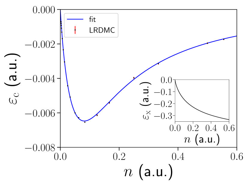
Figure 2: The $\varepsilon_{\mathrm{c}}$ (with associated error bars) for a set of HEGs over the density range used in the finite LDAs. The fit applied (solid blue) becomes exact in the known high-density and low-density limits. Inset: The $\varepsilon_{\mathrm{x}}$ curve in the HEG LDA.

The high-density limit (infinitely-weak correlation) of the parametrization is:

$$\varepsilon_{\mathrm{c}}(r_{\mathrm{s}}\rightarrow 0)=-A_{\mathrm{RPA}}r_{\mathrm{s}}^{2},$$ (6)

and its low-density limit (infinitely-strong correlation) is:

$$\varepsilon_{\mathrm{c}}(r_{\mathrm{s}}\rightarrow\infty)=-\frac{2E}{\alpha D}\frac{\ln(r_{\mathrm{s}})}{r_{\mathrm{s}}}.$$ (7)

Therefore, the parametric form in Eq. (5) correctly reproduces the expected behavior of the correlation energy density in the high-density limit Casula et al. (2006); Shulenburger et al. (2009) [$\varepsilon_{\mathrm{c}}\propto r_{\mathrm{s}}^{2}$] and low-density limit [$\varepsilon_{\mathrm{c}}\propto\ln(r_{\mathrm{s}})/r_{\mathrm{s}}$].

II.4 Comparison of 1e, 2e, 3e and HEG LDAs

Summing together the HEG exchange and correlation parametric fits, we can now compare the HEG LDA that we have developed against the three finite LDAs. The striking similarity between the four $\varepsilon_{\mathrm{xc}}$ curves can be seen in Fig. 3(a). While very similar in the low-density range, there are some differences between them. These are highlighted in Fig. 3(b) which, using the $1e$ LDA as a reference, plots its difference with the remaining LDAs. There is a competing balance between exchange and correlation. At low densities, these differences can be mainly attributed to $\varepsilon_{\mathrm{c}}$, which is entirely absent in the $1e$ LDA, and increases in magnitude as we progress to $2e$ to $3e$ to HEG (Fig. 4). As we move to higher densities in which the magnitude of $\varepsilon_{\mathrm{c}}$ decreases, and the magnitude of $\varepsilon_{\mathrm{x}}$ increases, the order of the four $\varepsilon_{\mathrm{xc}}$ curves reverses. They increasingly separate as we move to higher densities with the $1e$ LDA, which consists entirely of self-interaction correction, giving the largest magnitude for $\varepsilon_{\mathrm{xc}}$. By plotting the difference between the $1e$ LDA (where correlation is absent) and the exchange part of the HEG LDA (i.e., removing the correlation term), it can be seen that the $1e$ LDA yields a larger exchange energy density than the HEG LDA at all densities (Fig. 5).

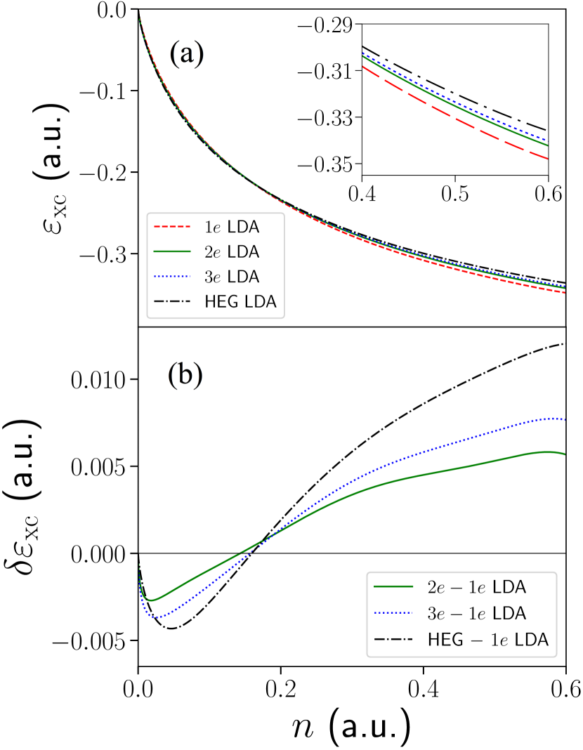
Figure 3: (a) The $\varepsilon_{\mathrm{xc}}$ curves in the $1e$ (dashed red), $2e$ (solid green), $3e$ (dotted blue) and HEG (dotted-dashed black) LDAs. Inset: Close-up of the four curves at higher densities. The similarity between them is striking, with a clear progression from $1e$ to $2e$ to $3e$ to HEG. (b) The $1e$ LDA is used as a reference here. Plotted is its difference ($\delta\varepsilon_{\mathrm{xc}}=\varepsilon_{\mathrm{xc}}-\varepsilon_{\mathrm{xc}}^{1e}$) with the $2e$ (solid green), $3e$ (dotted blue) and HEG (dotted-dashed black) LDAs.

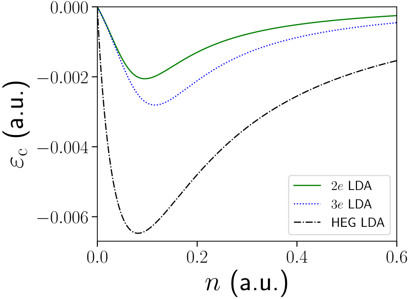
Figure 4: We calculate the exact $\varepsilon_{\mathrm{c}}$ for the $2e$ (solid green line) and $3e$ (dotted blue line) slab systems through Hartree-Fock calculations. We plot these against the $\varepsilon_{\mathrm{c}}$ curve in the HEG LDA (dotted-dashed black line). The $\varepsilon_{\mathrm{c}}$ in the HEG LDA is much larger ($\sim$2–3 that of the $3e$ LDA and $\sim$3–4 that of the $2e$ LDA). While not a perfect comparison due to the refinement process used in the construction of the finite LDAs, it gives a useful indication of the size of $\varepsilon_{\mathrm{c}}$ in their $\varepsilon_{\mathrm{xc}}$ curves.

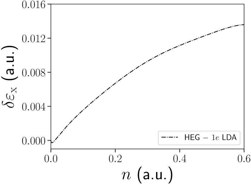
Figure 5: The $\varepsilon_{\mathrm{x}}$ curve in the $1e$ LDA ($\varepsilon_{\mathrm{x}}=\varepsilon_{\mathrm{xc}}$) is used as a reference here. Plotted is its difference ($\delta\varepsilon_{\mathrm{x}}=\varepsilon_{\mathrm{x}}-\varepsilon_{\mathrm{x}}^{1e}$) with the $\varepsilon_{\mathrm{x}}$ curve in the HEG LDA ($\varepsilon_{\mathrm{x}}=\varepsilon_{\mathrm{xc}}-\varepsilon_{\mathrm{c}}$). It can be seen that the $1e$ LDA yields a larger exchange energy density than the HEG LDA at all densities. Note: This is not true in the very low-density region ($n<0.012$), which we attribute to errors in the fits.

The refinement process used in the construction of the finite LDAs focused on giving the correct $E_{\mathrm{xc}}$ in the limit of the slab systems, but did not ensure that the correct $V_{\mathrm{xc}}$, and by extension electron density, were reproduced (a property of HEG LDAs). We find that the finite LDAs are completely inadequate at reproducing the densities of the slab systems. We compare the exact $V_{\mathrm{xc}}$ against $n$ and find that there is a high nonlocal dependence on $n$, implying that no local density functional can accurately reproduce $V_{\mathrm{xc}}$ and hence $n$ for the slab systems. In light of this, the success of the finite LDAs reported below is all the more surprising.

III Testing the LDAs

In the previous section we observed the close similarity between the four LDAs. In this section we apply them to a range of model systems in order to identify the differences between them.

III.1 Weakly correlated systems

System 1 (2e harmonic well). We first consider a pair of interacting electrons in a strongly confining harmonic potential well ($\omega=\frac{2}{3}$ a.u.) where correlation is very weak . We calculate the exact many-body electron density using iDEA, and compare it against the densities obtained from applying the LDAs self-consistently. There is a progression from the $1e$–$2e$–$3e$–HEG LDA and so we choose to plot the $1e$ and HEG LDA densities (i.e., the $2e$ and $3e$ LDA densities lie between these) against the exact [Fig. 6(a)]. Both LDAs match the exact density well, and so we plot their absolute errors ($\delta n=n^{\mathrm{LDA}}-n^{\mathrm{exact}}$) to more clearly identify their differences [Fig. 6(b)]. The $1e$ LDA has a slightly smaller net absolute error ($\int|\delta n|\ dx$). While the HEG LDA gives a slightly better electron density in the central region (dip in the density), the $1e$ LDA better matches the decay of the density towards the edges of the system, and perhaps more interestingly, the two peaks in the density where the self-interaction correction is largest.

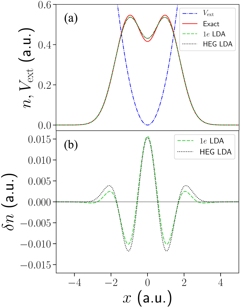
Figure 6: System 1 (two electrons in a harmonic potential well). (a) The external potential (dotted-dashed blue line), together with the exact electron density (solid red line), and the densities obtained from applying the $1e$ (dashed green line) and HEG (dotted black line) LDAs. Both LDAs are in very good agreement with the exact result. (b) The absolute error in the density ($\delta n=n^{\mathrm{LDA}}-n^{\mathrm{exact}}$) in the $1e$ (dashed green line) and HEG (dotted black line) LDAs, allowing their differences to be more clearly identified.

Due to the importance of energies in DFT calculations, we also compare the exact $E_{\mathrm{xc}}$ and total energy $E_{\mathrm{total}}$, with those obtained from applying the LDAs self-consistently (Table 4). While all the LDAs give good approximations to both quantities, there are some significant differences due to this system being dominated by regions of high density, and the $\varepsilon_{\mathrm{xc}}$ curves separating in this limit (see Fig. 3). As with the approximations to the electron density, there is a progression from the $1e$–$2e$–$3e$–HEG LDA, with the $1e$ LDA reducing the absolute errors ($\frac{\delta E_{\mathrm{xc}}}{E_{\mathrm{xc}}}$, $\frac{\delta E}{E}$) in the HEG LDA by a factor of $5-6$.

Table 4: Total energies and xc energies for the set of weakly correlated systems (1–3), from exact calculations and from applying the four LDAs self-consistently ($\delta E^{\mathrm{LDA}}=E^{\mathrm{LDA}}-E^{\mathrm{exact}}$). Estimated errors are $\pm$1 in the last decimal place, unless otherwise stated in parentheses.

System			$E_{\mathrm{total}}$ (a.u.)					$E_{\mathrm{xc}}$ (a.u.)
	Exact	$\delta E_{\mathrm{total}}^{1e}$	$\delta E_{\mathrm{total}}^{2e}$	$\delta E_{\mathrm{total}}^{3e}$	$\delta E_{\mathrm{total}}^{\text{HEG}}$	Exact	$\delta E_{\mathrm{xc}}^{1e}$	$\delta E_{\mathrm{xc}}^{2e}$	$\delta E_{\mathrm{xc}}^{3e}$	$\delta E_{\mathrm{xc}}^{\text{HEG}}$
$2e$ harmonic well	1.6932	0.0037	0.0126	0.0153	0.0211	$-0.6192$	0.0045	0.0137	0.0165	0.0225
$3e$ harmonic well	3.1875	$-0.0073$	0.0065	0.0108	0.0199	$-0.9305(5)$	$-0.0058(5)$	0.0085(5)	0.0129(5)	0.0223(5)
$2e$ double well	$-1.0301$	0.0237	0.0286	0.0296	0.0323	$-0.5349$	0.0256	0.0317	0.0331	0.0363

System 2 (3e harmonic well). Next, we consider a harmonic potential well with three electrons, but slightly less confining ($\omega=\frac{1}{2}$), in order to avoid an unphysically high electron density ($n>0.6$ a.u.). As in the $2e$ harmonic well system, we find a progression from the $1e$–$2e$–$3e$–HEG LDA, with all LDAs giving good electron densities (see Fig. 7(a) for the $1e$ and HEG LDA densities plotted against the exact). Again, the $1e$ LDA has the smallest net absolute error, and outperforms the rest of the LDAs in the regions where the density peaks [Fig. 7(b)].

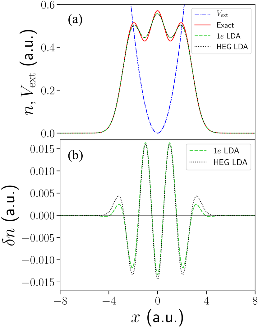
Figure 7: System 2 (three electrons in a harmonic potential well). (a) The external potential (dotted-dashed blue line), together with the exact electron density (solid red line), and the densities obtained from applying the $1e$ (dashed green line) and HEG (dotted black line) LDAs. Much like the $2e$ harmonic well system, both LDAs match the exact density well. (b) The absolute error in the density in the $1e$ (dashed green line) and HEG (dotted black line) LDAs. Again, the $1e$ LDA outperforms the HEG LDA in the density peaks, which is dominated by the self-interaction correction.

We also compare the exact $E_{\mathrm{xc}}$ and $E_{\mathrm{total}}$ against the LDAs (Table 4). All LDAs give good energies, with some noticeable differences between them due to this system being dominated by regions of high density, like in the $2e$ harmonic well system. However, the magnitude of $E_{\mathrm{xc}}$ in the $1e$ LDA is greater than the exact (i.e., it overestimates the amount of exchange $+$ correlation), and subsequently it gives a total energy lower than the exact. While the absolute error in $E_{\mathrm{xc}}$ for each LDA is similar to that in $E_{\mathrm{total}}$, this overestimation of exchange $+$ correlation in the $1e$ LDA results in the $2e$ LDA giving the best total energy.

III.2 A system dominated by the self-interaction correction

The self-interaction correction (SIC) is absent in xc functionals constructed from the HEG. However, the xc energy of the $1e$ slab systems (which were used to construct the $1e$ LDA) consists entirely of SIC. In the first two model systems, we found that the $1e$ LDA (and indeed the other finite LDAs) better describes the electron density in regions where the SIC is strongest, than the HEG LDA. We now investigate this further.

System 3 (2e double well). We choose a system with two electrons confined to a double-well potential. The wells are separated, such that the electrons are highly localized and can be considered as two separate subsystems [Fig. 8(a)]. This results in the Hartree potential being small outside of the wells, and being dominated by the electron self-interaction within the wells. Consequently, a large proportion of the xc potential is self-interaction correction. Applying the LDAs, we find the usual progression $1e$–$2e$–$3e$–HEG. Focusing on the peaks in the electron density, the $1e$ LDA substantially reduces the error present in the HEG LDA [Fig. 8(b)]. To understand this, we analyze the xc potential [Fig. 8(c)]. The $1e$ LDA better reproduces the large dips in $V_{\mathrm{xc}}$, corresponding to the peaks in the electron density. Hence, the SIC is more effectively captured.

Figure 8: System 3 (two electrons in a double-well potential). (a) The external potential (dotted-dashed blue line), together with the exact electron density (solid red line), and the densities obtained from applying the $1e$ (dashed green line) and HEG (dotted black line) LDAs. The wells are separated, such that the electrons are highly localized. (b) The absolute error in the density in the $1e$ (dashed green line) and HEG (dotted black line) LDAs. The $1e$ LDA is far superior in the regions where the density peaks, and hence where the Hartree potential is large and dominated by the electron self-interaction. (c) The exact xc potential (solid red line), and the xc potentials given by the $1e$ (dashed green line) and HEG (dotted black line) LDAs. The dips in $V_{\mathrm{xc}}$ are more closely matched by the $1e$ LDA due to it better capturing the self-interaction correction, present in the exact $V_{\mathrm{xc}}$.

While the LDA errors in $E_{\mathrm{xc}}$ are larger than in the first two systems, they are still small (4.8–6.8$\%$) (Table 4). The absolute errors in $E_{\mathrm{total}}$ are similar.

III.3 Systems where correlation is stronger

System 4 (2e atom). We now consider a system where the relative size of electron correlation increases significantly : two electrons confined to a softened atomiclike potential, $V_{\mathrm{ext}}=-(|ax|+1)^{-1}$, where $a=\frac{1}{20}$. Although we find the same progression ($1e$–$2e$–$3e$–HEG) as seen in the first three model systems, in which correlation was weak, all LDAs give inadequate electron densities. This can be seen by plotting the $1e$ and HEG LDA densities against the exact [Fig. 9(a)]. The LDAs give densities that are not even qualitatively correct, e.g., predicting a single peak in the center of the system, which is absent in the exact density. The net absolute errors are much larger than in the weakly correlated systems, however, the $1e$ LDA once again gives the smallest [Fig. 9(b)].

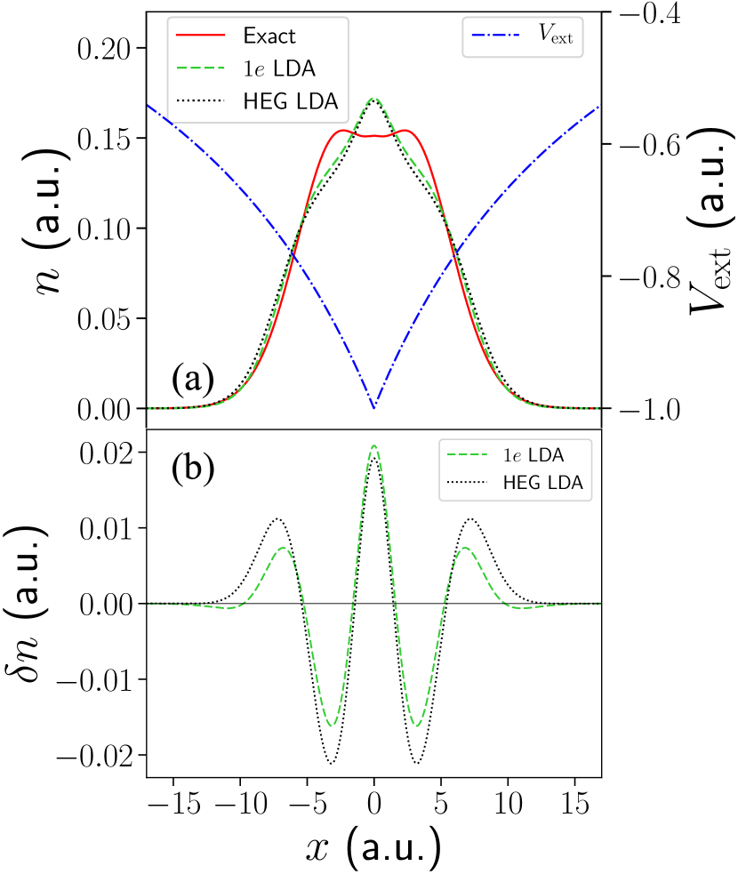
Figure 9: System 4 (two electrons in a softened atomiclike potential). (a) The external potential (dotted-dashed blue line), together with the exact electron density (solid red line), and the densities obtained from applying the $1e$ (dashed green line) and HEG (dotted black line) LDAs. Unlike in the weakly correlated systems, the LDAs give poor electron densities. (b) The absolute error in the density in the $1e$ (dashed green line) and HEG (dotted black line) LDAs. While the net absolute errors are much larger than in the weakly correlated systems, the $1e$ LDA still performs the best.

We find that although the LDA densities are poor, the xc energies are surprisingly good (Table 5). This can be attributed somewhat (see Sec. III.4 for investigation of further causes) to errors in the density being partially canceled by errors inherent in the approximate xc energy functional Kim et al. (2013). We infer this by noting the progression (HEG–$3e$–$2e$–$1e$) when we apply the LDAs to the exact density, in contrast to the self-consistent solutions in Table 5. As in the weakly correlated systems, the absolute errors in $E_{\mathrm{total}}$ are smaller than in $E_{\mathrm{xc}}$, due to a partial cancellation of errors from the Hartree energy component. It is much more apparent in this system due to the LDAs incorrectly predicting a central peak in the electron density [Fig. 9(a)].

Table 5: Total energies and xc energies for the set of strongly correlated systems (4-5), from exact calculations and from applying the four LDAs self-consistently ($\delta E^{\mathrm{LDA}}=E^{\mathrm{LDA}}-E^{\mathrm{exact}}$). Estimated errors are $\pm$1 in the last decimal place, unless otherwise stated in parentheses.

System			$E_{\mathrm{total}}$ (a.u.)					$E_{\mathrm{xc}}$ (a.u.)
	Exact	$\delta E_{\mathrm{total}}^{1e}$	$\delta E_{\mathrm{total}}^{2e}$	$\delta E_{\mathrm{total}}^{3e}$	$\delta E_{\mathrm{total}}^{\text{HEG}}$	Exact	$\delta E_{\mathrm{xc}}^{1e}$	$\delta E_{\mathrm{xc}}^{2e}$	$\delta E_{\mathrm{xc}}^{3e}$	$\delta E_{\mathrm{xc}}^{\text{HEG}}$
$2e$ atom	-1.5099	0.0053	0.0044	0.0032	0.0022	-0.3728	0.0084	0.0101	0.0099	0.0111
$3e$ atom	-2.3282(5)	0.0121(5)	0.0085(5)	0.0057(5)	0.0029(5)	-0.493(4)	0.029(4)	0.029(4)	0.027(4)	0.028(4)

System 5 (3e atom). Finally, we consider three electrons in an external potential of the same form as the $2e$ atom, but less confining, with $a=\frac{1}{50}$. Along with the usual progression ($1e$–$2e$–$3e$–HEG), we find a similar result to the $2e$ atom, with the LDAs giving poor electron densities [Fig. 10(a)]. Although the densities are qualitatively correct, unlike in the $2e$ atom, the LDAs significantly underestimate the peaks in the electron density. Subsequently, the absolute errors are very large [Fig. 10(b)]. The $1e$ LDA, along with giving the lowest net absolute error, most accurately reproduces the peaks in the density, where the SIC is largest.

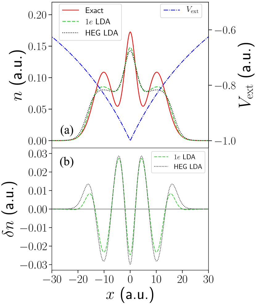
Figure 10: System 5 (three electrons in a softened atomiclike potential). (a) The external potential (dotted-dashed blue line), together with the exact electron density (solid red line), and the densities obtained from applying the $1e$ (dashed green line) and HEG (dotted black line) LDAs. Like in the $2e$ atom, the LDAs give poor electron densities. The $1e$ LDA more accurately reproduces the peaks in the density, where the SIC is largest. (b) The absolute error in the density in the $1e$ (dashed green line) and HEG (dotted black line) LDAs. Again, the net absolute errors are large, with the $1e$ LDA giving the smallest.

While the absolute errors in $E_{\mathrm{xc}}$ are larger than in the $2e$ atom, they are still small (Table 5). Again, this partially arises from applying approximate xc energy functionals to incorrect densities. As in the $2e$ atom, the absolute errors in $E_{\mathrm{total}}$ are much lower than those in $E_{\mathrm{xc}}$, due to a partial cancellation of errors from the Hartree energy component.

III.4 Cancellation of errors between exchange and correlation

HEG-based LDAs have been known to typically underestimate the magnitude of the exchange energy $E_{\mathrm{x}}$, while overestimating the magnitude of the correlation energy $E_{\mathrm{c}}$. Consequently, while the total $E_{\mathrm{xc}}$ is underestimated in magnitude, the approximation proves to be better than was originally expected due to a partial cancellation of errors.

We investigate how well our HEG LDA approximates $E_{\mathrm{x}}$ and $E_{\mathrm{c}}$ in the model systems, and how this contributes to accurate values for $E_{\mathrm{xc}}$. To do this we perform Hartree-Fock calculations for each of the model systems, and together with the exact solutions obtained through iDEA, are able to divide the exact $E_{\mathrm{xc}}$ into its exchange and correlation components. We then apply the HEG LDA, which is split into separate $E_{\mathrm{x}}$ and $E_{\mathrm{c}}$ functionals, for comparison (Table 6). In all systems, the HEG LDA underestimates the magnitude of $E_{\mathrm{x}}$, while it overestimates the magnitude of $E_{\mathrm{c}}$. However, due to the exchange energy being the dominant component of $E_{\mathrm{xc}}$, even in strongly correlated systems, this only leads to a partial cancellation of errors.

The $1e$ LDA yields a larger magnitude for $\varepsilon_{\mathrm{x}}$ than the HEG LDA across the entire density range studied (up to 0.6 a.u.) (Fig. 5), which arises from a better description of the SIC (Sec. III.2). In the $1e$ LDA correlation is absent. Consequently, the $1e$ xc energies that follow from Tables 4 and  5 can be considered as approximations to $E_{\mathrm{x}}$. We note that the $1e$ LDA substantially reduces the error in $E_{\mathrm{x}}$ that arises in the HEG LDA . We infer that this error reduction will also extend to the $2e$ and $3e$ LDAs.

Table 6: Exchange energies and correlation energies for all systems (1-5), from exact calculations and from applying the HEG LDA self-consistently ($\delta E^{\mathrm{LDA}}=E^{\mathrm{LDA}}-E^{\mathrm{exact}}$). Estimated errors are $\pm$1 in the last decimal place, unless otherwise stated in parentheses.

System	$\ \ \ \ \ \ \ \ \ \ \ \ \ \ \ \ \ \ \ \ \ \ \ \ \ \ \ \ E_{\mathrm{x}}\ \text{(a.u.)}$
	Exact	$\delta E_{\mathrm{x}}^{\text{HEG}}$
$2e$ harmonic well	$-0.6184$	$0.0268\rule{0.0pt}{11.19443pt}$
$3e$ harmonic well	$-0.9286(5)$	$0.0276(5)$
$2e$ double well	$-0.5349$	$0.0441$
$2e$ atom	$-0.3686$	$0.0185$
$3e$ atom	$-0.488(3)$	$0.041(3)\rule[-5.16663pt]{0.0pt}{0.0pt}$
System	$\ \ \ \ \ \ \ \ \ \ \ \ \ \ \ \ \ \ \ \ \ \ \ \ \ \ \ \ E_{\mathrm{c}}\ \text{(a.u.)}$
	Exact	$\delta E_{\mathrm{c}}^{\text{HEG}}$
$2e$ harmonic well	$-0.0008$	$-0.0043\rule{0.0pt}{11.19443pt}$
$3e$ harmonic well	$-0.0019$	$-0.0053$
$2e$ double well	$-0.0000$	$-0.0077$
$2e$ atom	$-0.0042$	$-0.0074$
$3e$ atom	$-0.0043(5)$	$-0.0142(5)$

IV Conclusions

We have constructed an LDA based on the homogeneous electron gas (HEG) through suitable quantum Monte Carlo techniques and find that it is remarkably similar in many regards to a set of three LDAs constructed from finite systems. Applying them to test systems to explore the differences between them, we find that the finite LDAs give better densities and energies in highly confined systems in which correlation is weak. Most interestingly, the LDA constructed from systems of just one electron most accurately describes the self-interaction correction. All LDAs give poor densities in systems where correlation is stronger, but give reasonably good energies, with the HEG LDA giving the best total energies. Across all test systems, the HEG LDA underestimates the magnitude of the exchange energy and overestimates the magnitude of the correlation energy, leading to a partial cancellation of errors. As a consequence of the finite LDAs giving a better description of the self-interaction correction, we infer that they would reduce the error in the exchange energy. Furthermore, we expect that finite LDA functionals will also provide a better treatment of the SIC for spinful electrons. Their derivation and usage could lead to an improved description of the electronic structure in a variety of situations, such as at the onset of Wigner oscillations.

Data created during this research is available by request from the York Research Database .