Neutron star merger GW170817 strongly constrains doubly coupled bigravity
Abstract
We study the implications of the recent detection of gravitational waves emitted by a pair of merging neutron stars and their electromagnetic counterpart, events GW170817 and GRB170817A, on the viability of the doubly coupled bimetric models of cosmic evolution, where the two metrics couple directly to matter through a composite, effective metric. We demonstrate that the bounds on the speed of gravitational waves place strong constraints on the doubly coupled models, forcing either the two metrics to be proportional at the background level or the models to become singly coupled. Proportional backgrounds are particularly interesting as they provide stable cosmological solutions with phenomenologies equivalent to that of CDM at the background level as well as for linear perturbations, while nonlinearities are expected to show deviations from the standard model.
I Introduction
The discovery of the late-time cosmic acceleration Riess et al. (1998); Perlmutter et al. (1999) (see Refs. Caldwell and Kamionkowski (2009); Weinberg et al. (2013); Joyce et al. (2015); Bull et al. (2016) for recent comprehensive reviews on the subject) triggered a wide interest in modifications of general relativity (see, e.g., Refs. Amendola and Tsujikawa (2010); Clifton et al. (2012) for reviews). Among these modifications to gravity, the bimetric theory of ghost-free, massive gravity is of particular interest. It stands out especially because of the strong theoretical restrictions on the possibilities for constructing a healthy theory of this type. Indeed, historically it has proven to be difficult to invent a healthy theory of massive, spin-2 field beyond the linear regime. The linearized theory has been known for a long time Fierz and Pauli (1939), while at the fully nonlinear level the theory has been discovered only recently by constructing the ghost-free111See, however, Ref. Koennig et al. (2016) for a discussion of the possibility of constructing viable theories of massive gravity in the presence of ghosts. theory of massive gravity de Rham and Gabadadze (2010); de Rham et al. (2011a); Hassan and Rosen (2011, 2012a); de Rham et al. (2012, 2011b); Hassan et al. (2012a); Hassan and Rosen (2012b); Hassan et al. (2012b); Hinterbichler and Rosen (2012). This development has also naturally led to the healthy theory of interacting, spin-2 fields, i.e. the theory of ghost-free, massive bigravity Hassan and Rosen (2012c); see Refs. de Rham (2014); Hinterbichler (2012); Schmidt-May and von Strauss (2016); Solomon (2015); Hinterbichler (2017) for reviews.
Over the past decade, there has been a substantial effort directed towards understanding the cosmological behavior of bimetric models,222See Ref. Luben et al. (2016) for viable background cosmologies of theories with more than two spin-2 fields. both theoretically and observationally. Particularly, it has been shown that bigravity admits Friedman-Lemaître-Robertson-Walker (FLRW) cosmologies333See Ref. Nersisyan et al. (2015) and references therein for bimetric cosmologies with other types of background metrics. which perfectly agree with cosmological observations at the background level Volkov (2012); Comelli et al. (2012a); von Strauss et al. (2012); Akrami et al. (2013a, 2015a); Könnig et al. (2014a); Enander et al. (2015a); Mortsell (2017). At the level of linear perturbations, the theory has been studied extensively in Refs. Comelli et al. (2012b); Khosravi et al. (2012); Berg et al. (2012); Könnig and Amendola (2014); Solomon et al. (2014); Könnig et al. (2014b); Lagos and Ferreira (2014); Cusin et al. (2015); Yamashita and Tanaka (2014); De Felice et al. (2014a); Fasiello and Tolley (2013); Enander et al. (2015b); Amendola et al. (2015); Johnson and Terrana (2015); Könnig (2015); Lagos and Ferreira (2017), and the cosmological solutions have been shown to suffer from either ghost or gradient instabilities, although the latter can be pushed back to arbitrarily early times by imposing a hierarchy between the two Planck masses of the theory Akrami et al. (2015b). It is also conjectured Mortsell and Enander (2015) that the gradient instability might be cured at the nonlinear level due to the presence of the Vainshtein screening mechanism Vainshtein (1972); Babichev and Deffayet (2013) in the theory. The version of the bimetric theory studied in all this work is the so-called singly coupled scenario, where the matter sector is assumed to couple to only one of the two metrics (spin-2 fields). The metric directly coupled to matter is called the physical metric, and the other spin-2 field, called the reference metric, affects the matter sector only indirectly and through its interaction with the physical metric.
In the absence of any theoretical mechanism that forbids the coupling of the matter fields directly to the reference metric, it is natural to go beyond the singly coupled scenarios and study doubly coupled models, where the two metrics couple to matter either directly or through a composite metric constructed out of the two spin-2 fields. This generalization might look even more natural since the gravity sector of ghost-free bigravity is fully symmetric in terms of the two metrics, and it might feel unnatural to impose the matter sector to break this symmetry by coupling only to one metric.444Note also that such theories do not necessarily violate the equivalence principle, and if they do, this may not be an issue. For discussions on the violation of the equivalence principle in theories with both metrics minimally coupled to matter, see Refs. Akrami et al. (2013b, 2014). For theories with a composite metric coupled to matter the (weak) equivalence principle is not violated, as all particles move along the geodesics of the composite metric. Theories of doubly coupled massive gravity and bigravity, and, in particular, their cosmologies, have also been extensively studied Hassan et al. (2013); Akrami et al. (2013b); Tamanini et al. (2014); Akrami et al. (2014); Yamashita et al. (2014); de Rham et al. (2015, 2015); Hassan et al. (2014); Enander et al. (2015a); Solomon et al. (2015); Schmidt-May (2015); de Rham et al. (2014); Gümrükçüoğlu et al. (2015a); Heisenberg (2015a); Gümrükçüoğlu et al. (2015b); Hinterbichler and Rosen (2015); Heisenberg (2015b, c); Lagos and Noller (2016); Melville and Noller (2016); Heisenberg and Refregier (2016); Brax et al. (2017a, b, c). It has been shown, particularly, that the dangerous Boulware-Deser (BD) ghost Boulware and Deser (1972) reemerges almost always if the same matter fields couple to both metrics. One interesting exception has been proposed in Ref. de Rham et al. (2015), where an acceptable doubly coupled theory of bimetric gravity has been constructed with matter coupled to a composite metric of the form
| (1) |
with and being the two metrics of the theory, and and being two arbitrary constants. Clearly, setting to ( to ) turns the doubly coupled theory into a singly coupled one with () being the physical metric. Even though in this case the BD ghost is not completely removed from the theory, it is effective only at high energies above the cutoff scale of the theory,555This cutoff scale for massive gravity, corresponding to the strong-coupling scale, is , where is the graviton mass and is the Planck mass. The cutoff scale can be higher for bigravity Akrami et al. (2015b). making it a valid effective field theory at low energies.
This doubly coupled theory has been shown to provide viable and interesting cosmological solutions at the background level Enander et al. (2015a); Lagos and Noller (2016), with linear perturbations that are stable at least around specific cosmological backgrounds Comelli et al. (2015) (see also Refs. Gümrükçüoğlu et al. (2015b); Brax et al. (2017a, b, c)). In particular, in contrast to the singly coupled theory, this double coupling admits combinations of proportional metrics at the background level, and interestingly, the effective metric always corresponds to the massless fluctuations around such backgrounds, i.e. it satisfies the linearized Einstein equations. It can further be considered as a nonlinear massless spin-2 field Schmidt-May (2015). This means that around proportional backgrounds the theory is equivalent to general relativity at the background level as well as for linear perturbations, and differences from general relativity are expected only at the nonlinear level, at least in the sector coupled to matter. The immediate implication of this feature is that doubly coupled bigravity admits viable and stable cosmologies at least for proportional metrics, which are potentially distinguishable from standard cosmology in the nonlinear regime.666The linear cosmological perturbations for doubly coupled bigravity around proportional, FLRW backgrounds separate into two decoupled sectors. The first (visible) sector coupled to matter is equivalent to general relativity. The second (hidden) sector is decoupled from matter and is not free from some instabilities. The most dangerous one Comelli et al. (2015); Brax et al. (2017a) occurs for vectors, which have a gradient instability in the radiation era. This may jeopardize the perturbativity of the models very early on in the Universe. On the other hand, however, the doubly coupled models with a mass are expected to have an ultraviolet (UV) cutoff scale of order , which is low and prevents any reliable description of the physics of bigravity when the horizon scale becomes smaller than . Strictly speaking, for bimetric theories is the cutoff scale in the decoupling limit, and the cutoff scale for the full theory can be higher, contrary to massive gravity. However, since the decoupling limit is not well defined above , we expect the entire theory to need modifications. The scale happens at a redshift of order which is just before big bang nucleosynthesis. The unknown UV completion of doubly coupled bigravity would certainly affect the early-Universe instability. In the late Universe as we consider here, no instability is present and the decoupled sector can be safely ignored for proportional backgrounds. As we show in this paper, proportional metrics are extremely interesting also from the point of view of gravitational waves (GWs), as they are the only cases that survive after the recent measurements of the speed of gravity in addition to the singly coupled models. This provides us with a unique class of bimetric models that are healthy and compatible with all cosmological observations as well as gravitational wave constraints.
Given the large number of possible modifications to gravity, it is natural to ask how all these theories can be tested and potentially falsified. Several high-precision large-scale structure surveys are planned to come into operation in the very near future, and therefore most attempts so far have focused on studying the cosmological implications of such theories in a hope that the future cosmological surveys will be sufficiently sensitive to judge against or for many of these theories. Notably, however, the recent detection of the GWs originating from a pair of merging neutron stars and the simultaneous detection of their electromagnetic counterpart, events GW170817 Abbott et al. (2017) and GRB 170817A Goldstein et al. (2017), have proven to be able to provide us with an immense amount of knowledge about the landscape of the possible theories of gravity (mainly) through the strong bounds that they have placed on the speed of GWs Creminelli and Vernizzi (2017); Sakstein and Jain (2017); Ezquiaga and Zumalacarregui (2017); Baker et al. (2017); Nojiri and Odintsov (2017); Boran et al. (2018); Amendola et al. (2017); Crisostomi and Koyama (2017a); Langlois et al. (2017); Gumrukcuoglu et al. (2017); Heisenberg and Tsujikawa (2017); Kreisch and Komatsu (2017); Dima and Vernizzi (2017); Peirone et al. (2017); Crisostomi and Koyama (2017b); Linder (2018); Kase and Tsujikawa (2018); Battye et al. (2018) (see also Refs. Lombriser and Taylor (2016); Brax et al. (2016); Lombriser and Lima (2017); Pogosian and Silvestri (2016); Bettoni et al. (2017) for discussions on the consequences of such strong bounds for classes of modified theories of gravity prior to the actual observations).
GWs in bigravity have been studied in Refs. De Felice et al. (2014b); Saltas et al. (2014); Cusin et al. (2015); Narikawa et al. (2015); Amendola et al. (2015); Johnson and Terrana (2015); Max et al. (2017a); Brax et al. (2017b); Nishizawa (2017); Max et al. (2017b), although they have been investigated for the doubly coupled models only in Ref. Brax et al. (2017b). In the literature, bigravity models are often considered to be on the safe side with respect to the bounds placed by current observations of GWs. While this holds for singly coupled models, we show in this paper that the bounds on the speed of GWs severely constrain the parameter space of the doubly coupled scenarios. We particularly show that the models which survive the bounds from current gravitational wave observations are the ones for which the two background metrics are proportional, or for the choices of the parameters of the model that render it singly coupled.
We first derive, analytically, the conditions under which bimetric models are safe in terms of the gravitational wave measurements. We then perform a Markov chain Monte Carlo (MCMC) analysis of the parameter space of doubly coupled bigravity by imposing the constraints from geometrical measurements of cosmic history, now taking into account also the constraints from gravitational wave observations. We illustrate that this numerical analysis confirms our analytical arguments.
The paper is organized as follows: In Sec. II we summarize the basics of doubly coupled bigravity and its cosmology, and present the equations necessary for studying the background cosmological evolution. Section III discusses the evolution equations and the speed of GWs in the theory and presents the cosmological conditions that result in the speed equal to the speed of light. Section IV provides the results of our MCMC scans, and our conclusions are given in Sec. V. Finally, in Appendix A we derive the cosmological evolution equations for tensor modes in detail, at the level of the field equations as well as the action.
II Cosmology of doubly coupled bigravity
The theory of doubly coupled bigravity can be formulated in terms of an action of the form de Rham et al. (2015); Enander et al. (2015a)
| (2) |
where and are the two metrics of the theory with determinants and , respectively, and standard Einstein-Hilbert kinetic terms. plays the role of the Planck mass,777It should be noted that the theory can be formulated in terms of two separate Planck masses and corresponding to the and sectors, respectively. As has been shown in Ref. Enander et al. (2015a), the effective metric in this case does not include any free parameters and has the fixed form . We have chosen the formulation in terms of with and being present explicitly since it shows the singly coupled limits of the theory more clearly. are the elementary symmetric polynomials of the matrix (see Ref. Hassan and Rosen (2012c) for their detailed definitions), and the quantities are five free parameters determining the strength of the possible interaction terms. The parameter sets the mass scale of the interactions and is not an independent parameter of the theory as it can be absorbed into the parameters; needs to be of the order of , the present value of the Hubble parameter , in order for the theory to provide self-accelerating solutions consistent with observational data. Matter fields have been shown collectively by , which couple to the effective metric defined in Eq. (1) in terms of and and the two coupling parameters and .
In order to study the cosmological implications of the theory, we assume the background metrics and to have the FLRW forms
| (3) | ||||
| (4) |
where is the cosmic time, and are the lapse functions for and , respectively, and and are the corresponding scale factors, all functions of only.
Using the forms (3) and (4) for the background metrics and , Eq. (1) fixes the form of the effective metric to
| (5) |
where Enander et al. (2015a)
| (6) | ||||
| (7) |
are the lapse and the scale factor of the effective metric, respectively. The dynamics of and are governed by their Friedmann equations, which take the forms
| (8) | ||||
| (9) |
where
| (10) |
are the Hubble parameters for and , respectively, is the energy density of matter and radiation, the dot denotes a derivative with respect to , and
| (11) |
is the ratio of the two scale factors and . We have also fixed to in the two Friedmann equations, as we are interested in self-accelerating solutions for which .
In addition to the two Friedmann equations (8) and (9), the consistency of the theory requires the Bianchi constraint Enander et al. (2015a)
| (12) |
to be satisfied.888Note that the Bianchi constraint gives two branches of solutions. The one we consider here is the so-called dynamical branch. See Refs. Enander et al. (2015a); Lagos and Noller (2016) for the discussion of the second, algebraic branch. Having introduced the effective lapse and scale factor and , one can naturally introduce an effective Hubble parameter associated with the effective metric ,
| (13) |
which satisfies its own effective Friedmann equation Enander et al. (2015a),
| (14) |
where we have also introduced
| (15) | ||||
| (16) |
Equation (14) is obtained by adding the two Friedman equations (8) and (9), and applying the Bianchi constraint (12). The effective Hubble parameter can be written in terms of or as
| (17) |
In addition to the Friedmann equation for , by again using the Bianchi constraint (12) and now subtracting the two Friedmann equations (8) and (9) we arrive at the algebraic condition
| (18) |
The energy-momentum tensor for matter and radiation is covariantly conserved with respect to the effective metric, which means that the energy density satisfies the continuity equation
| (19) |
This motivates us to introduce , the number of -folds in terms of the effective scale factor , as a time coordinate. In terms of , we can recover the usual behavior of the matter and radiation energy densities
| (20) |
assuming that these two components are conserved separately. Here, and are the current values of the energy densities of matter and radiation, respectively.
It is easy to show that the coupling parameters and affect observables only though their ratio , as we can assume without loss of generality999This is indeed the case because the singly coupled bigravity theories with either of the metrics being coupled to matter are completely equivalent. and then rescale by a factor of . Later in this paper, when discussing the constraints, we use this rescaling freedom and introduce a new parameter
| (21) |
which plays the role of the only extra parameter for doubly coupled models compared to the singly coupled ones. Identifying the effective Planck mass with the usual Planck mass , our doubly coupled bimetric model now possesses six free parameters, with , and . For now, however, let us keep both and explicit as it allows us to see explicitly the duality properties of the background dynamics equations as well as the equations governing the propagation speed of the GWs.
Before we proceed with our studies of gravitational waves in the next sections, let us emphasize an important property of the cosmological evolution equations that we presented in this section. As can be seen easily at the level of the action, the theory is symmetric under the simultaneous interchanges , and (or ) and therefore all the dynamical equations remain unchanged Enander et al. (2015a). More concretely, let us consider two sets of parameters and , where are some particular values of the parameters. It is easy to show that the solution of Eq. (18) for with the first set of parameter values is identical to the solution for the quantity with the second set of parameter values. Now if we rewrite Eq. (14) in terms of (note that we do not make an actual interchange , and we only rewrite the equations in terms of ) then for the two distinct sets of parameter values given above the two Friedmann equations are precisely the same. This, for example, implies that when scanning the single-parameter submodel with all the parameters turned off except the space of all the cosmological solutions that we obtain is fully equivalent to the one for the submodel with only turned on (given that we leave and , or equivalently , free). This is a useful observation and helps us reduce the number of cases studied in the next sections.
III The speed of gravitational waves
The spectrum of bimetric theories of gravity contains two gravitons, one massive and one massless, with five and two degrees of freedom, respectively. In order to study the properties of gravitational waves one needs to focus only on tensor modes, i.e. the helicity-2 modes of the gravitons. Massless and massive gravitons have two helicity-2 modes each. It is important to note that in general the two metrics of the theory, and , each contain a combination of massive and massless modes, and therefore the evolution equations for the and tensor modes do not represent directly the evolution of the tensor modes for massive and massless modes. Indeed, it is not possible in general to diagonalize the spectrum of spin-2 perturbations into mass eigenstates, and therefore the notion of mass does not make sense around arbitrary backgrounds Schmidt-May (2015). One can specifically show Schmidt-May (2015) that mass eigenstates can be defined only around proportional metrics by computing the spectrum of linear perturbations and comparing their equations with those of linearized general relativity. Proportional metrics are therefore extremely interesting from this point of view, as the notion of spin-2 mass eigenstates does not exist for other types of backgrounds. As we mentioned in Sec. I, contrary to the theory of singly coupled bigravity, the doubly coupled theory admits proportional backgrounds (both in vacuum and in the presence of matter). It can be shown additionally that the effective metric of the theory, , corresponds exactly to the massless mode around such backgrounds, while the massive mode is fully decoupled Schmidt-May (2015). This immediately implies that the speed of GWs around proportional backgrounds measured by any detectors must be equal to the speed of light since the detectors see only the effective metric. Such solutions are therefore safe regarding the bounds from the GW observations. We show later in this paper that, in addition to the singly coupled corner of the theory, proportional backgrounds are indeed the only solutions that survive the bounds from GWs.
As detailed in Appendix A, the propagation equations for the and tensor modes and around the cosmological backgrounds are
| (22) | |||||
| (23) |
Here, the prime denotes a derivative with respect to the conformal time corresponding to the effective metric, , which is defined through
| (24) |
With this time coordinate the background effective metric reads
| (25) |
First note that we have written the equations in terms of the time coordinate corresponding to the effective metric and not or , because the effective metric is the one that couples to matter and therefore plays the role of the physical spacetime metric, used for measuring distances and time intervals. In addition, we chose to work with the conformal time because in this coordinate light rays travel as in a Minkowski spacetime, making a particularly useful time coordinate for identifying the propagation speeds of the gravitational waves.
We can now read off from Eqs. (22) and (23) the propagation speeds and for the gravitational waves and , respectively, as101010Note that since we are interested in bigravity solutions with the interaction scale in order to explain cosmic acceleration, the effects of the graviton mass on the speed of the gravitational waves are several orders of magnitude smaller than the sensitivity of current GW detectors. We therefore fully ignore the direct contributions from the mass terms to the speed.
| (26) | |||||
| (27) |
The ratio of the two speeds is a coordinate-independent quantity and is given by
| (28) |
As we see later, the quantity plays a crucial role in the rest of the discussions in this paper.
One should note again that in doubly coupled bigravity one measures neither nor separately. The tensor modes measured by gravitational wave detectors are the ones corresponding to the effective metric . These observable modes can be written in terms of and , the tensor modes of the and metrics respectively, as
| (29) |
where
| (30) | |||||
| (31) | |||||
| (32) |
with (see Appendix A for details).
The recent measurements of the GWs from neutron star mergers have imposed incredibly tight constraints on the speed of gravitons. The relative difference between the two speeds must be smaller than , which is practically . Let us therefore assume that the speed of GWs is exactly the same as the speed of light, and study its implications.
The mentioned bound on the speed of GWs tells us that at least one of the quantities and should be unity (note that in our units). The reason for this is that at least one of the or graviton modes should have traveled with the speed of light when arriving at the detector. Keeping this in mind let us first assume that
-
•
we are in a truly doubly coupled regime (i.e. and ) ,
-
•
is a finite and nonzero quantity,
-
•
and are finite and nonzero.
Let us further set and write the two speeds and as
| (33) | |||||
| (34) |
Now it is clear that, first of all, when , both and become unity. Moreover, when either or is unity, we necessarily have . This then tells us very strongly that in the case of finite and nonzero , and , and under the assumption of and , is the necessary and sufficient condition for compatibility with the GW experiments.
Let us now discuss the validity of the assumptions that we made above. From the Friedmann equation (14) we see that both infinite and zero values of lead to singularity in the observable Hubble function unless either or is , i.e. the theory is singly coupled. This means that for physical solutions in the doubly coupled regime is necessarily finite and nonzero. Additionally, if while is finite and nonzero, we see that while 111111Here we have used the expression for the effective lapse function which is not equal to unity unless we are in the singly coupled regime of . In exactly the same way the case of while simultaneously is finite and nonzero is excluded. In principle, one should also consider the cases with one of the lapse functions going to infinity while their ratio is fixed.121212Otherwise, obviously, they cannot satisfy the gauge fixing condition . Note however that such cases not only produce unphysical propagation speeds in both and sectors, but they also remove the second-order time derivatives in the tensor propagation equations, hence rendering the initial data from the past lost at one particular instant in time (when the divergence happens). Based on these considerations we can conclude that the cases with or are excluded.
Finally, as it is expected, in the singly coupled case (say, and ), we have and , which is the only observationally important speed in this limit. It is very important to note that in such a singly coupled limit or are not necessarily dangerous since the potentially singular terms containing (as well as the terms containing , which are dangerous when ) are multiplied by both and and therefore vanish in either the case of or . Putting all these discussions together we arrive at an important statement: the propagation of gravitational waves in doubly coupled bigravity is viable if and only if or we are in a singly coupled regime.
It is important to note that the current bounds on the speed of GWs have been placed through the observations at very low redshifts (), i.e. at almost the present time. This means that, strictly speaking, the viability conditions we discussed above are required to hold only at , including the condition . Let us for now assume that the constraint on the speed of GWs is valid not only in the present epoch but it applies also to the earlier epochs of the Universe, i.e. we assume at all times. Later on, when we discuss our numerical analysis, we show a rather vigorous feature of the theory that imposing will force to be unity at all redshifts.
Imposing at all times tells us that the two background metrics and should be proportional. This can easily be seen by setting in Eq. (28) and noting that , resulting in
| (35) |
with being some (constant) proportionality factor. In order to understand under which circumstances these proportional solutions exist, let us consider the early-time and late-time asymptotic limits of Eq. (18). By taking the future asymptotic limit, with , we obtain
| (36) |
for the value of in the far future, . Note that being a solution of this time-independent equation means that it is a constant. This in turn means that the two metrics are necessarily proportional in the far-future limit. Additionally, the early-Universe limit of Eq. (18) fixes the value of to either or . The latter does not give viable cosmologies Enander et al. (2015a), and therefore is the only viable early-time limit. Restricting to the solutions for which does not exhibit any singular behavior Enander et al. (2015a), one can show that should monotonically evolve between and over the history. The monotonicity of implies that when the two limiting values and coincide, i.e. when , we have constant over the entire history of the Universe and hence the background metrics are proportional in that case.
Based on the discussions above, we can now formulate the necessary and sufficient conditions for the two background metrics to be proportional:
-
1.
Background solutions are proportional if and only if is given by at all times, where . Note that one does not need to check whether this condition holds at all times; as we argued above, because of the monotonicity of , having even at one instant in time, other than the asymptotic past, is sufficient for the condition to be satisfied at all times.
-
2.
Equivalently, the background solutions are proportional if and only if the parameters of the model solve the algebraic equation
(37)
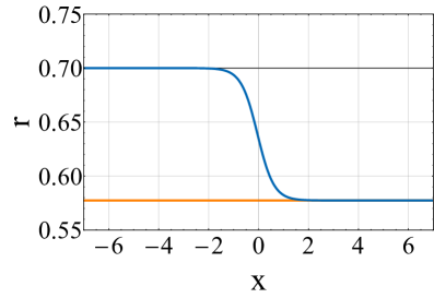
We demonstrate these conditions in Fig. 1 by plotting the dependence of on the number of -folds , with the present time given by , for a single-interaction-parameter scenario where only is turned on while . The blue curve corresponds to a case where does not satisfy the special tuning condition for proportional metrics. The curve exhibits two constant- epochs. The far-past epoch corresponds to (the horizontal, thin, black line), while the far-future limit is given by the solution of Eq. (36) for which regardless of the value of . The orange curve corresponds to a case where is chosen such that it is the solution of Eq. (36), i.e. . The value of is not relevant for the arguments here because in this case the asymptotic value is independent of the value of (the value of is always independent of the values of parameters). In order to illustrate our arguments, we have chosen two different values of for producing the two curves (blue and orange). As expected, they agree in the far-future limit, even though the values of are different for the two curves.
As we see in the next section, bigravity models for which only one of the parameters is turned on are particularly interesting. For those cases the proportional background solutions correspond to the following values of the parameter :
-
1.
or only: ,
-
2.
only: ,
-
3.
only: ,
-
4.
only: .
Note that and therefore in these cases are independent of the value of the corresponding parameter. Note also that, as we discussed in the previous section, the single-parameter models with only or turned on are identical, as long as (or equivalently ), justifying the values and for in these models. In addition, it is interesting to notice that for the and only models, proportional backgrounds do not exist, as in those cases is forced to be vanishing, and therefore the theory becomes singly coupled.
All these cases of proportional background metrics with only one of the parameters being nonzero can be verified easily by applying the Bianchi constraint to the Friedmann equations (8) and (9), obtaining
| (38) | ||||
| (39) |
In general, we have two dynamical variables and , which are determined by the two independent, dynamical equations (38) and (39). Now, if the two metrics are proportional, this means that and are also proportional, and is a constant. We then have effectively only one dynamical variable, or , and the two dynamical equations (38) and (39) must be identical. This means that the right-hand sides of the two equations should be identically the same. Now, setting all the parameters to , except for either of , , or , we immediately arrive at the values for and presented above for these three cases.
Now turning back to the condition for the speed of the gravitational waves to be identical to the speed of light, we argued that what is strictly needed is to have , as the speed of GWs has been measured only at the present epoch . If, additionally, the parameters of the model giving satisfy the algebraic equation (37) then they lead to proportional background solutions and the condition is satisfied at all times, implying necessarily that at all times. The question of whether a set of parameters giving (hence ) while not satisfying Eq. (37) can happen in our doubly coupled bigravity models cannot be answered based on our analytical arguments here, and needs a numerical scanning of the parameter space. In principle it could be possible that the two background metrics are not proportional while becomes unity at the present epoch simply as a coincidence for a specific combination of the parameters. We however demonstrate later that for all the models that we study in this paper the cosmologically viable solutions with also satisfy Eq. (37), implying at all times, and therefore the proportionality of the background metrics.
IV MCMC scans and observational constraints
In this section we present the results of a set of MCMC scans of the parameter space of doubly coupled bigravity when different sets of parameters are allowed to vary while the rest are fixed to . We should first emphasize that we do not intend here to perform a detailed parameter estimation of the model using cosmological observations. This has been done in Ref. Enander et al. (2015a) using the geometrical constraints on cosmic histories at the background level.131313Note, however, that the MCMC scans presented in Ref. Enander et al. (2015a) include only single- models, while in the current paper we consider also the cosmological constraints on two-parameter models. We are rather interested in studying the impact of the constraints from the measurements of gravitational waves and the bounds on their speed on the cosmologically viable regions of the parameter space. We first perform MCMC scans of the models using similar cosmological data sets as those used in Ref. Enander et al. (2015a). The geometrical constraints that we consider are a combination of the observed angular scales of the cosmic microwave background anisotropies Ade et al. (2016), the supernovae redshift-luminosity relation Betoule et al. (2014), the measurements of the baryon acoustic oscillations (BAO) Beutler et al. (2011); Blake et al. (2011); Anderson et al. (2013, 2014); Ross et al. (2015), and the local measurement of the Hubble constant Riess et al. (2016). Our scans provide a set of points in the parameter space of the models all of which are in good agreement with cosmological observations. We have checked that our results are in perfect agreement with the results of Ref. Enander et al. (2015a) for the cases studied in that paper. We then explore the implications of imposing the GW constraints on the points, and investigate whether and how strongly the cosmologically viable regions are affected by the GW observations.
Our full bigravity model contains seven free parameters, as far as our MCMC scans are concerned. These include the five parameters for the interaction terms, the ratio of the couplings of the two metrics to matter , and the present value of the matter density parameter , defined as
| (40) |
Note that one should not necessarily expect to obtain a value for similar to the best-fit one in the standard model of cosmology, CDM, for a bigravity model that fits the data well, even for proportional backgrounds where the interaction terms contribute with a -like constant to the Friedmann equation. The reason, as explained in Ref. Enander et al. (2015a) in detail, is the extra factor appearing in the matter density term of the Friedmann equation. We see below that indeed in some cases the viable points in the parameter space give values for that are significantly smaller than the CDM value of .
For each point in the parameter space of the theory we also output the corresponding values of , , and , all evaluated at the present time. These allow us to check which parts of the parameter space agree with the observational constraint (or ), and to verify explicitly the conditions on and . We particularly use the quantity as a measure of how fit a point is to the observational constraints on the speed of GWs.
We perform our MCMC scans for various submodels, namely the single-parameter141414This is only a terminological convention here, and strictly speaking, our single-parameter models have two free parameters, as is always a free parameter of the models. models of , , and (with other being set to zero in each case), and the two-parameter models of , , , and . One should note that, as we discussed before, the single-parameter models of and are identical to the and models, respectively, because of the duality properties of the theory. In addition, for the same reason, each one of the other two-parameter models is equivalent to one of the two-parameter models considered here, and their phenomenologies are therefore already captured. Our objective in this paper is not to perform a detailed and extensive statistical analysis of the entire parameter space of doubly coupled bigravity, and we are mainly interested in a qualitative understanding of the implications of the GW observations for the viability of the theory, which can very well be captured in the studies of single-parameter and two-parameter cases. We therefore do not discuss three- or higher-parameter models. As we see later, although the constraints are quite strong for most of these cases, the parameter space in some models still allows viable cosmologies, and clearly, by increasing the number of free parameters one expects to enlarge the number of possibilities for finding viable scenarios within the model. We leave a detailed statistical analysis of the full model for future work.
IV.1 One-parameter models
model: Let us first emphasize that, contrary to singly coupled bigravity, in the doubly coupled theory the parameters and are no longer the explicit cosmological constants corresponding to the two metrics and . The reason is that matter couples to the effective metric , which is a combination of and . This can be seen explicitly by looking at the effective Friedmann equation (14) and comparing it with Eqs. (8) and (9). In addition, in the singly coupled theory, where matter couples to, say, , behaves as the matter vacuum energy in the action of the theory, as it appears in the interaction terms as (note that ). In the doubly coupled theory, however, all the interaction parameters directly receive contributions from quantum matter loops, and the definition of vacuum energy is more subtle than in the singly coupled theory. It is therefore interesting to study a single-parameter, doubly coupled model with only turned on, while all the other parameters are set to : for the singly coupled case this is nothing but CDM. The cosmology of this model in doubly coupled bigravity has been studied in Ref. Enander et al. (2015a). We reproduce and show the cosmological constraints on the three parameters , , and in the upper panels of Fig. 2, which are in full agreement with the results of Ref. Enander et al. (2015a). Note that corresponds to the singly coupled scenario, which reduces to CDM for this -only model.

Let us now look at the lowest panel of Fig. 2, where the present value of has been depicted versus . This plot shows that in order for the model to be cosmologically viable and simultaneously predict gravitational waves with the speed equal to the speed of light (i.e. for at least one of the two quantities and to be unity), is required to be , which in turn implies that the model needs to be singly coupled. In this case is forced to be vanishing, although is no longer a meaningful quantity as there is no interaction between and , and completely decouples from the theory. This all tells us that the model satisfies the cosmological and gravitational wave constraints only in its singly coupled limit, which is equivalent to CDM. We do not see any cases of proportional metrics in this model, as such cases should also give GWs consistent with observations. Let us take a closer look at this and understand why such a situation does not happen in the model by looking again at the condition for proportional background metrics. As we argued in the previous section, for proportional backgrounds must satisfy Eq. (37), while . Setting all parameters to except for , we arrive at . First of all, this is exactly what we see in the middle, left panel of Fig. 2 for and . Additionally, we are back to the condition that corresponds to a single coupling. This means that the model does not admit any sets of (nontrivial) proportional backgrounds, unless we consider to be proportional to with a vanishing proportionality factor. The fact that this is a peculiar case can also be seen by looking at the middle, right panel of Fig. 2, which shows versus . is always negative, which means that the condition for proportional backgrounds, , can never be satisfied.
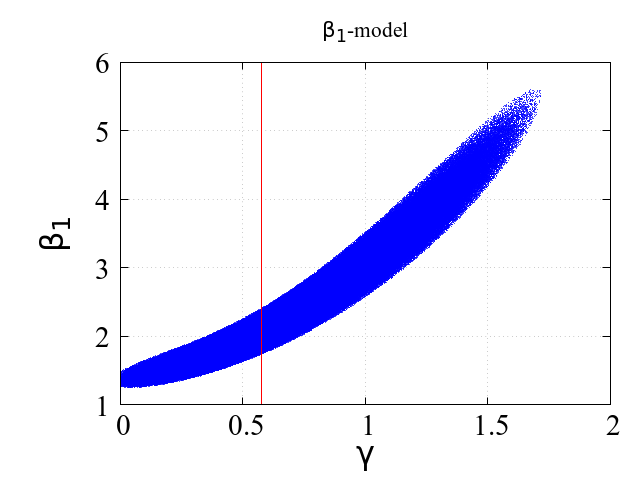
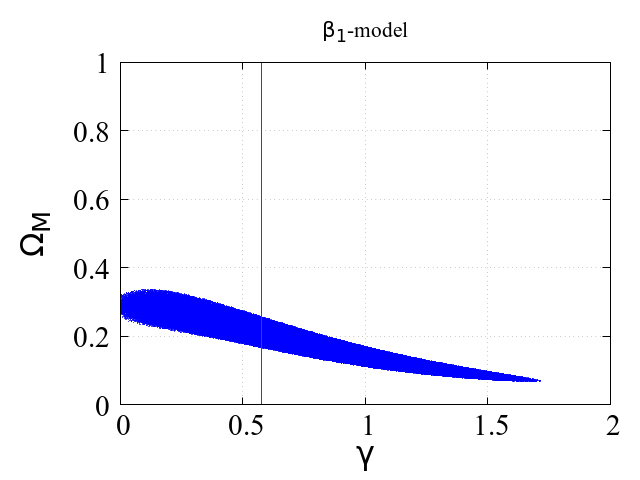
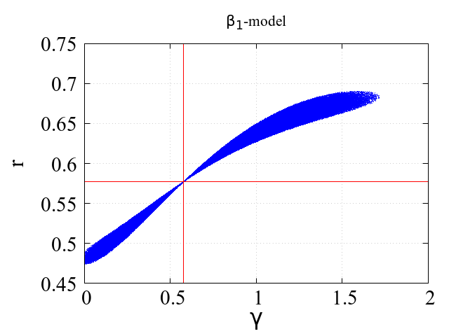
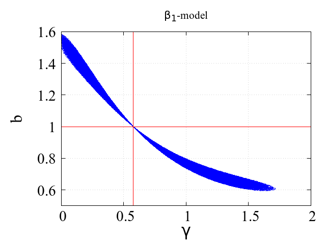
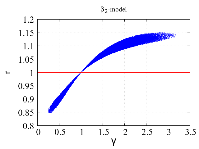
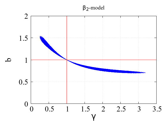
model: Here we turn on only the parameter and set to all the other interaction parameters . From our discussions in the previous section, we expect this submodel to give the speed of gravity waves equal to the speed of light for the cases with , where the background metrics are proportional, as well as for the singly coupled corners with . The lowest panel of Fig. 3 presents the dependence of on the value of as a result of our numerical scans. We first notice that no viable combinations of the parameters provide and both larger or smaller than the speed of light, as is always negative or . The plot also shows two points with , one of which being the obvious limit of single coupling with , and the other one, as expected, corresponding to the case of proportional backgrounds with , depicted by the vertical, red line. This becomes more clear by looking at the middle panels of Fig. 3, showing and versus . The red lines in the plots show that indeed corresponds to and , as expected. Also note that is always positive for all the cosmologically viable points in the parameter space of this model. Finally, the upper panels of Fig. 3 show the constraints on and versus , with the vertical lines again showing the condition for the two background metrics to be proportional, with giving : all the points residing on the lines are viable. Although most of the original, cosmologically viable points are now excluded and the model is highly constrained, our results show that there still remains some freedom in choosing for the fixed . It is also interesting to note that the preferred values of are smaller than the CDM value of . In summary, as expected, the viable points in the parameter space of the model correspond to the scenarios which do not represent the full dynamics of the doubly coupled model. One remaining region is the singly coupled limit, and the other one corresponds to the cases where the background metrics are proportional, and we again effectively have only one dynamical metric at work. In this latter case, the model is effectively equivalent to CDM, at the level of the background (and linear perturbations Schmidt-May (2015)).

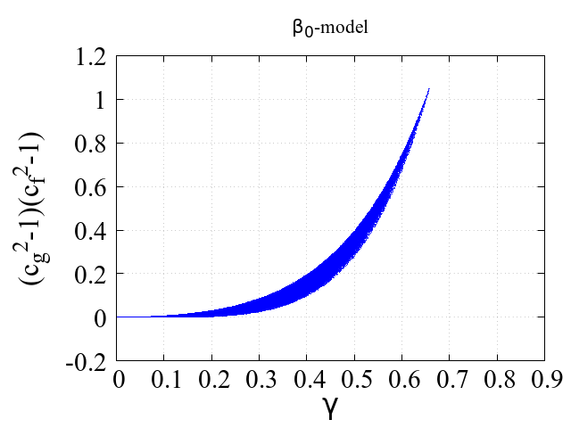
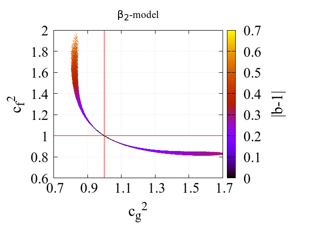
model: Fig. 4 presents the results of our MCMC scans for the model with only turned on. All the panels clearly show that the singly coupled subset of the parameter space (with ) is not viable cosmologically as there are no points with that fit the data. This is in agreement with the results of Ref. Akrami et al. (2015a). The model, however, provides excellent fits to the data for . Looking now at the lowest panel of Fig. 4, we see that the only points in the parameter space that are consistent with today, i.e. with the bounds from the GW observations, are the ones for which , meaning that the metrics are proportional. These points correspond to (see the middle, right panel). This is in agreement with our findings in the previous section for the model, with for proportional metrics. For all the other cosmologically viable points the tensor modes of one of the two metrics and travel faster and the other ones travel slower than light. Finally, the upper panels show the constraints on the model parameters and , with again lower preferred values for compared to CDM.


IV.2 Two-parameter models
Let us now turn on two of the interaction parameters and let them vary. As we argued earlier, many of these submodels are physically equivalent because of the symmetry of the theory. We therefore study four representative cases of , , , and models. Note that even though for example the model with only turned on is identical to the model with only turned on, when the two parameters are both nonzero the resulting two-parameter model can in general be very different from the single-parameter ones, with generally richer phenomenologies. The reason is that the two parameters can take two different values, making the model different from the cases with only one of the parameters left free.
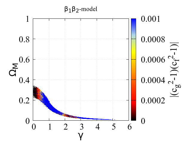
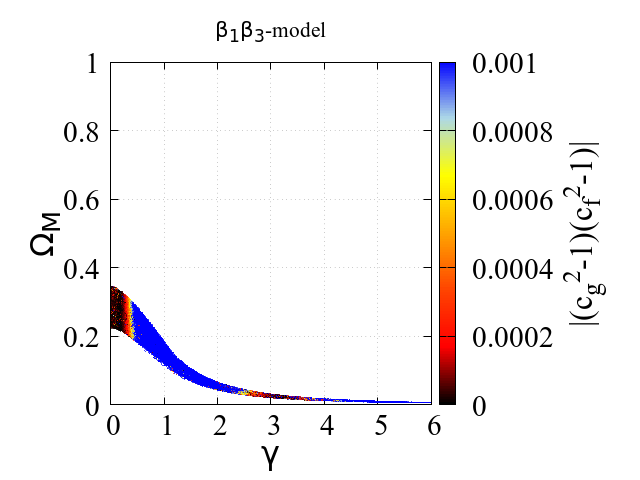
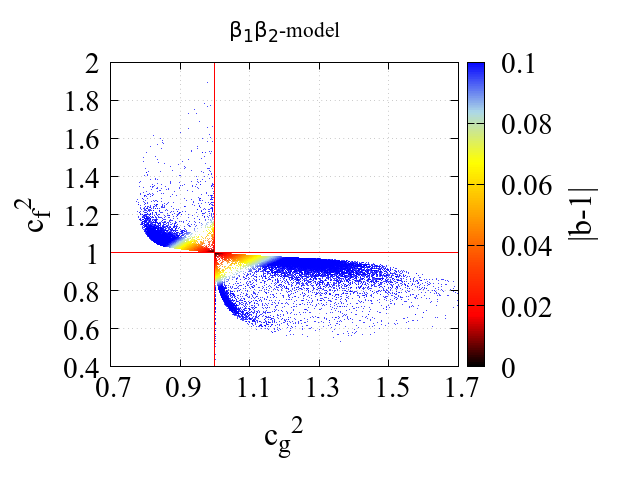
The results of our MCMC scans for these models are presented in Fig. 5, where the quantities and (both computed at the present time) are given in terms of the coupling ratio . The color code shows the values of .

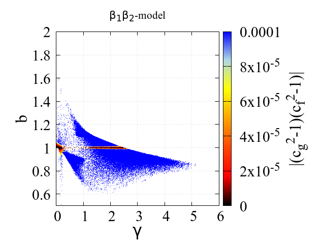


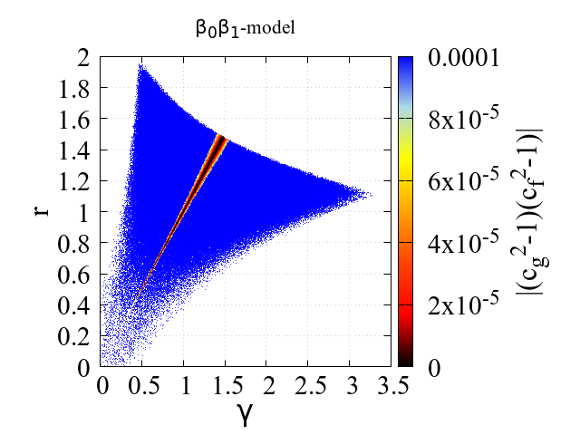
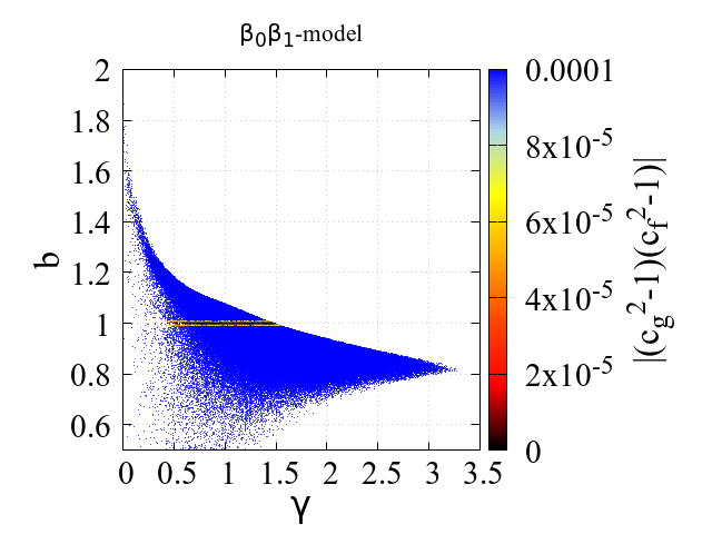
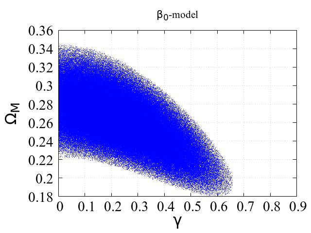
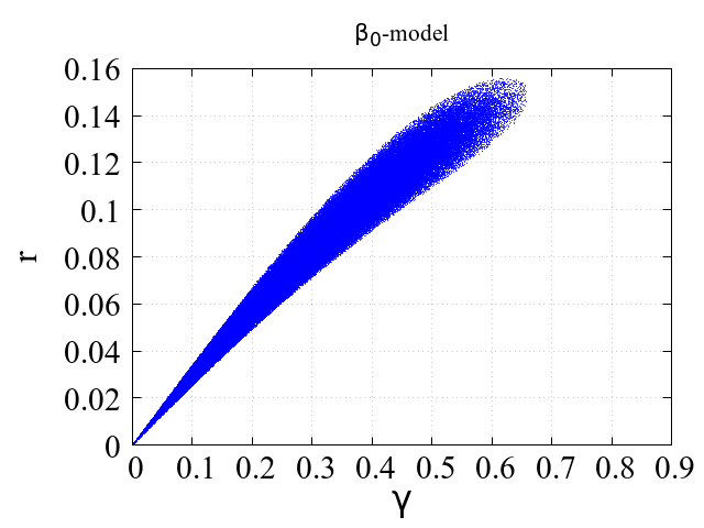
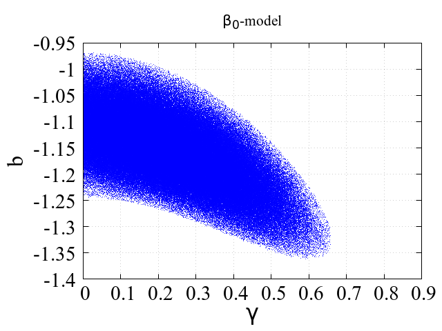
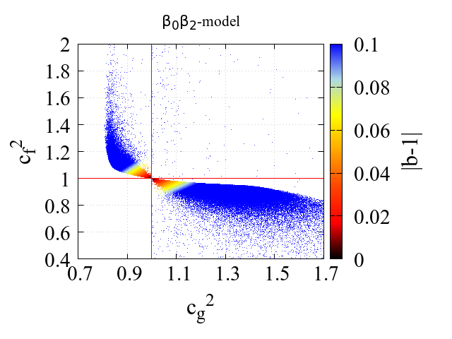
and models: Looking at the four upper panels of Fig. 5 for these models, we observe an interesting feature. The points in the parameter space of both models for which is small seem to be residing on a thin region, shown with shades of black. All the other points are excluded by gravitational waves, although they give good fits to the cosmological observations. Let us try to understand this favored, thin region. We argued in the previous section that if becomes equal to , even at one point over the history (in addition to far in the past), the two background metrics of the model should be proportional at all times. This means that in particular if a point in the parameter space requires at the present time, that point should correspond to proportional metrics. Now looking at the plots of versus for both and models, we see that the very thin, linelike part of the favored region is indeed the line. This therefore shows that one main region with corresponds in fact to the cases with proportional backgrounds. This can be seen further by looking at the plots of versus . The thin, black line now corresponds to , as expected for proportional metrics. The other tiny region with being very small is the one in the vicinity of . Note that this region is not clearly visible in the plots because it is a highly thin region perpendicular to the axis and is difficult to depict. The plots are therefore consistent with our analytical arguments in the previous section that only singly coupled submodels or the ones with the two background metrics being proportional are consistent with the speed of gravitational waves being the same as the speed of light. The observations of gravitational waves therefore highly constrain these two bigravity models as it was the case also for the single-parameter models. Note that the upper cuts in the plots are the result of the finite ranges which we have chosen in our MCMC scans for the parameters. We have checked that by increasing these ranges the cuts on the plots systematically move upwards, but the main features do not change—the thin, favored regions only extend to larger and . Finally, we show in the upper panels of Fig. 6 the constraints on , the present value of the matter density parameter, for the and models. We can clearly see that there are two regions with being close to , one in the vicinity of , corresponding to the singly coupled corner of the theory, and the other one with far from , corresponding to proportional backgrounds. It is interesting to note that the values of for the latter case which are consistent with GW constraints are significantly smaller than the best-fit value of for the CDM model.
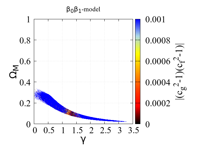
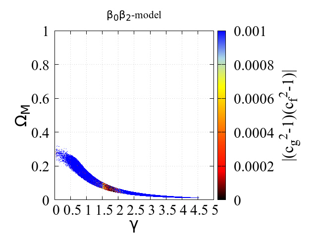
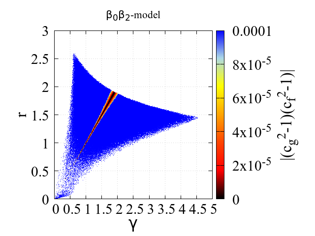
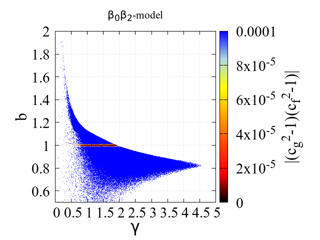
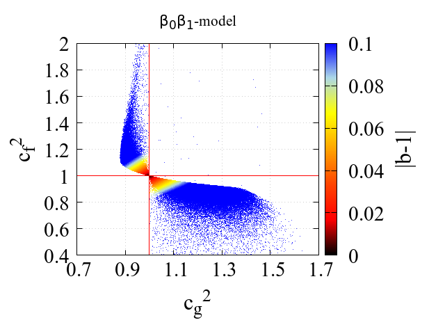
and models: Let us now investigate the two and models, by studying the four lower panels of Fig. 5. Overall, the same features as in the previous models of and can be seen here, especially that proportional backgrounds survive the bounds on the speed of gravitational waves. This can be seen again as a thin line. There is however an interesting difference in these two models compared to the previous ones.
The parameters and being in each case while is also set to corresponds to CDM, with playing the role of the cosmological constant. We may therefore expect a large concentration of cosmologically viable points in the region. Even though this region does exist, as is better visible for the model, the majority of the viable points seem to be clustering around large , especially for the model. In order to understand this, let us look at Figs. 2 and 4 for the single-parameter, and models. It is clear from these figures that the models act in opposite ways. While the model favors small , the model does not admit smaller than . Although we may expect the entire range of to be covered by turning on both of the parameters, our numerical investigations show that the points in the parameter space of the model fit the cosmological observations better when is not and is large. That is why the density of the points in the figures is higher at large , where the model deviates significantly from the singly coupled scenario. The same holds for the model, although in that case the singly coupled submodel is less disfavored. This can be understood by looking at Fig. 3 for the single-parameter, model, where the plots show that small are cosmologically viable, contrary to the model.


IV.3 Further remarks
Before we end the discussions of our numerical investigation, let us present the results of our MCMC scans for all the two-parameter models of , , , and , as well as the single-parameter models of and , now in terms of the speed of the gravitational waves corresponding to the two metrics of the theory, and . These have been shown in Fig. 7. In order to see how far each cosmologically viable point in the parameter space is from the proportional backgrounds, we color code the points by the value of . All the quantities , , and have been computed at the present time, i.e. at .
First of all, the plots confirm our analytical arguments in the previous section that having () automatically implies (), unless the theory is singly coupled. In addition, the plots also show that is equivalent to , i.e. it corresponds to proportional backgrounds, as expected. These can clearly be seen in all the panels. Let us first focus on the single-parameter cases of and , i.e. the first two upper panels of Fig. 7. The intersections of the and lines in both models correspond to the proportional backgrounds, as at those points. In addition, for the model we see that there are points for which while takes larger values (). This is fully consistent with our previous discussions that the model admits cosmologically viable singly coupled solutions—these are the points with and therefore consistent with the GW observations. The model, on the other hand, does not allow singly coupled models consistent with cosmological observations, and we therefore do not see any points in the panel of Fig. 7 with and . Note that in our analysis where we work with instead of and , the singly coupled models are captured only by being the physical metric, as we fix to unity and therefore . That is why we do not see any points with and for the model. Let us now focus on the two-parameter models. As we discussed above, the and models do not favor singly coupled solutions, and that is why we do not see many points in the corresponding panels of Fig. 7 with and . Out of the two other two-parameter models of and , we see that in the latter case there is a concentration of cosmologically favored points along the vertical line of even with in the and panels of Fig. 7. This is again consistent with our findings above that singly coupled bigravity is not disfavored in the model.
V Conclusions
In this paper, we have extensively studied the implications of the recently detected gravitational waves from a neutron star merger and their electromagnetic counterpart on the viability of the doubly coupled theory of bimetric gravity, and have identified the regions of the parameter space that are consistent with both cosmological observations and gravitational wave measurements. We have been interested in models that provide an alternative explanation for the late-time acceleration of the Universe, and therefore require an interaction (or mass) scale of the order of the present value of the Hubble parameter (i.e. ). Our studies have been based on both an analytical investigation of cosmic evolution and propagation of tensor modes in the theory, as well as a numerical exploration of the parameter space of the model using MCMC scans. We have demonstrated that the only regions of the parameter space that survive both the cosmological and gravitational wave constraints are those with the two background metrics being proportional or the singly coupled submodels. Our findings therefore demonstrate that the theory is strongly constrained by the bounds on the speed of gravity waves if it is considered as the mechanism behind cosmic acceleration.
The cases with proportional backgrounds are particularly interesting for various reasons Schmidt-May (2015). First of all, the background evolution of the Universe as well as linear perturbations mimic those of the CDM model, and the model is therefore consistent with all the existing cosmological observations. This also means that the model does not suffer from any ghost or gradient instabilities, which are the typical drawbacks of singly coupled cosmological scenarios, in the (visible) sector where the cosmological perturbations are coupled to matter. The model is however expected to deviate from general relativity, and therefore CDM, at the nonlinear level and in the early Universe such as the radiation era, where a vector instability in the (hidden) sector decoupled from matter would have to be cured by an as yet unknown UV completion. The expected nonlinear deviations from general relativity in the late Universe open up an interesting route for further tests of the theory using the observations of structure formation and evolution at nonlinear scales. In addition, graviton mass eigenstates can be diagonalized only around the proportional backgrounds, and therefore the notion of spin-2 mass makes sense only in those cases—singly coupled bigravity does not admit proportional metrics in the presence of matter. Moreover, the effective metric of the doubly coupled theory, which is the one that couples to matter, corresponds to the massless modes at the linear level, while the massive modes are fully decoupled; the massive and massless modes however mix at the nonlinear level.
We therefore conclude that the recent, tight constraints on the speed of gravitational waves leave us with a highly constrained corner of bigravity which is theoretically healthy at low energies151515These models are valid below the cutoff scale and are therefore well suited for a description of the late-time Universe. and observationally viable. It remains to be seen whether the model will also fit the cosmological observations at the nonlinear level, or will be ruled out; we leave the investigation of this interesting question for future work.
Acknowledgements.
Y.A. acknowledges support from the Netherlands Organization for Scientific Research (NWO) and the Dutch Ministry of Education, Culture and Science (OCW), and also from the D-ITP consortium, a program of the NWO that is funded by the OCW. A.C.D is partially supported by STFC under Grants No. ST/L000385/1 and No. ST/L000636/1. V.V. is supported by a de Sitter PhD fellowship of NWO. This work is supported in part by the EU Horizon 2020 research and innovation program under the Marie-Sklodowska Grant No. 690575. This article is based upon work related to the COST Action Grant No. CA15117 (CANTATA) supported by COST (European Cooperation in Science and Technology).Appendix A Tensor modes
Here we present the detailed derivation of tensor perturbations and their propagation equations in doubly coupled bimetric gravity. We present the calculations in the metric formalism at the level of the equations of motion, as well as at the action level, both in metric and vierbein formalisms.
Derivation from equations of motion. — Here our starting point is the full (modified) Einstein equations for the two metrics and , which are given by (see Ref. Schmidt-May (2015) for details)
| (41) | |||||
and
| (42) | |||||
where and are the Einstein tensors for and , respectively, is the stress-energy tensor corresponding to the effective metric , and the square-root matrices and are defined through
| (43) | |||||
| (44) |
Now, the linear metric perturbations for and tensor modes and can be written as
| (45) | |||||
| (46) | |||||
Plugging these into Eqs. (43) and (44) we find
| (47) |
and
| (48) |
for the square-root matrices at the linear order.
Having these expressions for and , the nonvanishing parts of the tensor sector of the effective metric can be shown to be
| (49) | |||||
| (50) | |||||
By using Eqs. (47) and (48) in the field equations we recover Friedmann equations at the background level, while at the linear order we obtain the propagation equations for the tensor modes and ,
| (51) | |||||
| (52) |
where
| (53) | |||||
| (54) |
with here being the pressure of the matter sector.
It should be noted that these two propagation equations can be written in a form that manifestly shows the symmetry of the interaction terms (i.e. the symmetry of the mass matrix). This can be seen by rewriting the propagation equations as
| (55) | |||||
| (56) | |||||
where now the same factor of appears in front of in the first equation and in front of in the second equation.
Derivation of the quadratic action. — In order to facilitate the comparison with the results of Refs. Brax et al. (2017a, b) let us also present the calculation of the graviton mass matrix at the level of the action. In this analysis we ignore the matter sector, i.e. we study a fully dark energy dominated epoch.
First of all, by varying the background part of the action with respect to the lapses and scale factors we recover the background equations of motion
| (57) | |||||
| (58) | |||||
| (59) | |||||
Our objective here is to obtain the mass terms of the gravitational waves. In principle, the calculation of the quadratic action is straightforward, but the subtle point here is that besides the potential terms of bigravity, also the two Einstein-Hilbert terms contribute with additional terms quadratic in and . Let us exemplify this by looking at the kinetic term of the -sector. First of all, there is a contribution from the volume factor, which reads as
| (60) |
where is the background part of the Ricci scalar, which is given by
| (61) |
Additional contributions come from some of the terms in the perturbed part of the Ricci scalar, namely from
| (62) |
where
| (63) |
The corresponding contributions to the mass matrix are given by
| (64) |
Note that we needed to divide by a factor of in the last expression, because in the original terms only the variations with respect to the fields under the time derivatives could contribute to the mass terms in the equations of motion.
These contributions should be added to the contributions from the potential terms. In order to find the latter we also need the second-order piece of the matrix, the nonvanishing components of which are found to be
| (65) | |||||
| (66) |
Combining all the potential terms and dropping an overall factor of from the action we obtain the graviton mass terms
| (67) |
where the mass matrix is found to be
| (68) | |||||
Note particularly that we have recovered the same interaction terms as in Eqs. (55) and (56).
In Refs. Brax et al. (2017a, b) the interaction sector has been written in terms of the constrained metric vierbeins as
| (69) | |||||
where the tetrad fields (or vierbeins) are defined through
| (70) |
Here labels the two metrics, , and are the covariant indices, and and are the indices in the local Lorentz frame. The interaction matrix is fully symmetric and its components in terms of the parameters are given by
| (71) | |||||
| (72) |
with the other components being trivially related to the ones above due to the total symmetry of the matrix.
In order to derive the mass sector of the quadratic action in the vierbein formalism we first derive the tensor perturbations of the vierbeins by linearizing Eq. (70). As a result, for the matrix we have
| (73) |
The total mass matrix is built up from two different parts of the action as before.
The first (diagonal) contribution comes from the Einstein-Hilbert terms in the action, and is given by
| (74) |
where we have found that
| (75) | |||||
| (76) |
Here and are the same functions as in Eq. (63).
The second part comes from the expansion of the potential term (69) to second order in the gravitons. Direct calculation gives
| (77) |
where
| (78) | |||||
| (79) | |||||
| (80) | |||||
Adding the two sectors, making use of the background equations of motion (57)-(59), and dropping an overall factor of from the action, we retrieve the action (67) with the mass matrix given exactly by (68).
The massless and massive modes. — The dynamics of the two gravitons can be better understood by switching to the canonically normalized basis
| (81) |
where and we have defined
| (82) |
In this new basis the mass matrix reads
| (83) |
where . In this basis the graviton equations read
| (84) |
where we have identified the speeds of the waves in the effective conformal time (for which photons have a normalized speed ),
| (85) |
It is easy to see that this mass matrix always has a massless and a massive eigenmode given by
| (86) |
with eigenmass square being
| (87) |
where the factor of has been included to comply with the usual definition for the mass of graviton in FLRW spacetimes. In the case of proportional metrics, when , the above mass eigenvectors reduce to
| (88) |
which guarantees that one can diagonalize the system of dynamical equations (84) by simply adding linear combinations of the two propagation equations with constant coefficients.
Now, one can see that the canonically normalized massless eigenmode is associated to the effective graviton modes. Indeed, first of all from Eqs. (49) and (50) we see that , with . The canonically normalized version of this field is the massless mode . The massive mode, on the other hand, corresponds to the difference .
Combining the equations of motion in (84) appropriately, we obtain
| (89) | |||||
| (90) |
Here we have used the fact that for the proportional backgrounds we have if we pick the lapses as . Moreover, recalling that
| (91) |
we see that . The first of these dynamical equations is the propagation equation of gravitons in general relativity, with the gravitons being massless but receiving a “pseudo”mass of the form . The second one is the propagation equation for a massive graviton of mass . Notice that for both modes the speed of propagation is , and that (91) implies that the light cones for gravitons and photons coincide.
References
- Riess et al. (1998) Adam G. Riess et al. (Supernova Search Team), “Observational evidence from supernovae for an accelerating universe and a cosmological constant,” Astron. J. 116, 1009–1038 (1998), arXiv:astro-ph/9805201 [astro-ph] .
- Perlmutter et al. (1999) S. Perlmutter et al. (Supernova Cosmology Project), “Measurements of Omega and Lambda from 42 high redshift supernovae,” Astrophys. J. 517, 565–586 (1999), arXiv:astro-ph/9812133 [astro-ph] .
- Caldwell and Kamionkowski (2009) Robert R. Caldwell and Marc Kamionkowski, “The Physics of Cosmic Acceleration,” Ann. Rev. Nucl. Part. Sci. 59, 397–429 (2009), arXiv:0903.0866 [astro-ph.CO] .
- Weinberg et al. (2013) David H. Weinberg, Michael J. Mortonson, Daniel J. Eisenstein, Christopher Hirata, Adam G. Riess, and Eduardo Rozo, “Observational Probes of Cosmic Acceleration,” Phys. Rept. 530, 87–255 (2013), arXiv:1201.2434 [astro-ph.CO] .
- Joyce et al. (2015) Austin Joyce, Bhuvnesh Jain, Justin Khoury, and Mark Trodden, “Beyond the Cosmological Standard Model,” Phys. Rept. 568, 1–98 (2015), arXiv:1407.0059 [astro-ph.CO] .
- Bull et al. (2016) Philip Bull, Yashar Akrami, et al., “Beyond CDM: Problems, solutions, and the road ahead,” Phys. Dark Univ. 12, 56–99 (2016), arXiv:1512.05356 [astro-ph.CO] .
- Amendola and Tsujikawa (2010) L. Amendola and S. Tsujikawa, Dark Energy: Theory and Observations (Cambridge University Press, 2010).
- Clifton et al. (2012) Timothy Clifton, Pedro G. Ferreira, Antonio Padilla, and Constantinos Skordis, “Modified Gravity and Cosmology,” Phys.Rept. 513, 1–189 (2012), arXiv:1106.2476 [astro-ph.CO] .
- Fierz and Pauli (1939) M. Fierz and W. Pauli, “On relativistic wave equations for particles of arbitrary spin in an electromagnetic field,” Proc.Roy.Soc.Lond. A173, 211–232 (1939).
- Koennig et al. (2016) Frank Koennig, Henrik Nersisyan, Yashar Akrami, Luca Amendola, and Miguel Zumalacarregui, “A spectre is haunting the cosmos: Quantum stability of massive gravity with ghosts,” JHEP 11, 118 (2016), arXiv:1605.08757 [gr-qc] .
- de Rham and Gabadadze (2010) Claudia de Rham and Gregory Gabadadze, “Generalization of the Fierz-Pauli Action,” Phys.Rev. D82, 044020 (2010), arXiv:1007.0443 [hep-th] .
- de Rham et al. (2011a) Claudia de Rham, Gregory Gabadadze, and Andrew J. Tolley, “Resummation of Massive Gravity,” Phys.Rev.Lett. 106, 231101 (2011a), arXiv:1011.1232 [hep-th] .
- Hassan and Rosen (2011) S.F. Hassan and Rachel A. Rosen, “On Non-Linear Actions for Massive Gravity,” JHEP 1107, 009 (2011), arXiv:1103.6055 [hep-th] .
- Hassan and Rosen (2012a) S.F. Hassan and Rachel A. Rosen, “Resolving the Ghost Problem in non-Linear Massive Gravity,” Phys.Rev.Lett. 108, 041101 (2012a), arXiv:1106.3344 [hep-th] .
- de Rham et al. (2012) Claudia de Rham, Gregory Gabadadze, and Andrew J. Tolley, “Ghost free Massive Gravity in the Stückelberg language,” Phys.Lett. B711, 190–195 (2012), arXiv:1107.3820 [hep-th] .
- de Rham et al. (2011b) Claudia de Rham, Gregory Gabadadze, and Andrew J. Tolley, “Helicity Decomposition of Ghost-free Massive Gravity,” JHEP 1111, 093 (2011b), arXiv:1108.4521 [hep-th] .
- Hassan et al. (2012a) S.F. Hassan, Rachel A. Rosen, and Angnis Schmidt-May, “Ghost-free Massive Gravity with a General Reference Metric,” JHEP 1202, 026 (2012a), arXiv:1109.3230 [hep-th] .
- Hassan and Rosen (2012b) S.F. Hassan and Rachel A. Rosen, “Confirmation of the Secondary Constraint and Absence of Ghost in Massive Gravity and Bimetric Gravity,” JHEP 1204, 123 (2012b), arXiv:1111.2070 [hep-th] .
- Hassan et al. (2012b) S.F. Hassan, Angnis Schmidt-May, and Mikael von Strauss, “Proof of Consistency of Nonlinear Massive Gravity in the Stückelberg Formulation,” Phys.Lett. B715, 335–339 (2012b), arXiv:1203.5283 [hep-th] .
- Hinterbichler and Rosen (2012) Kurt Hinterbichler and Rachel A. Rosen, “Interacting Spin-2 Fields,” JHEP 1207, 047 (2012), arXiv:1203.5783 [hep-th] .
- Hassan and Rosen (2012c) S.F. Hassan and Rachel A. Rosen, “Bimetric Gravity from Ghost-free Massive Gravity,” JHEP 1202, 126 (2012c), arXiv:1109.3515 [hep-th] .
- de Rham (2014) Claudia de Rham, “Massive Gravity,” Living Rev.Rel. 17, 7 (2014), arXiv:1401.4173 [hep-th] .
- Hinterbichler (2012) Kurt Hinterbichler, “Theoretical Aspects of Massive Gravity,” Rev.Mod.Phys. 84, 671–710 (2012), arXiv:1105.3735 [hep-th] .
- Schmidt-May and von Strauss (2016) Angnis Schmidt-May and Mikael von Strauss, “Recent developments in bimetric theory,” J. Phys. A49, 183001 (2016), arXiv:1512.00021 [hep-th] .
- Solomon (2015) Adam R. Solomon, Cosmology Beyond Einstein, Ph.D. thesis, Cambridge U. (2015), arXiv:1508.06859 [gr-qc] .
- Hinterbichler (2017) Kurt Hinterbichler, “Cosmology of Massive Gravity and its Extensions,” in 51st Rencontres de Moriond on Cosmology La Thuile (2017) arXiv:1701.02873 [astro-ph.CO] .
- Luben et al. (2016) Marvin Luben, Yashar Akrami, Luca Amendola, and Adam R. Solomon, “Cosmology with three interacting spin-2 fields,” Phys. Rev. D94, 043530 (2016), arXiv:1604.04285 [astro-ph.CO] .
- Nersisyan et al. (2015) Henrik Nersisyan, Yashar Akrami, and Luca Amendola, “Consistent metric combinations in cosmology of massive bigravity,” Phys. Rev. D92, 104034 (2015), arXiv:1502.03988 [gr-qc] .
- Volkov (2012) Mikhail S. Volkov, “Cosmological solutions with massive gravitons in the bigravity theory,” JHEP 1201, 035 (2012), arXiv:1110.6153 [hep-th] .
- Comelli et al. (2012a) D. Comelli, M. Crisostomi, F. Nesti, and L. Pilo, “FRW Cosmology in Ghost Free Massive Gravity,” JHEP 1203, 067 (2012a), arXiv:1111.1983 [hep-th] .
- von Strauss et al. (2012) Mikael von Strauss, Angnis Schmidt-May, Jonas Enander, Edvard Mörtsell, and S.F. Hassan, “Cosmological Solutions in Bimetric Gravity and their Observational Tests,” JCAP 1203, 042 (2012), arXiv:1111.1655 [gr-qc] .
- Akrami et al. (2013a) Yashar Akrami, Tomi S. Koivisto, and Marit Sandstad, “Accelerated expansion from ghost-free bigravity: a statistical analysis with improved generality,” JHEP 1303, 099 (2013a), arXiv:1209.0457 [astro-ph.CO] .
- Akrami et al. (2015a) Yashar Akrami, Tomi S. Koivisto, and Marit Sandstad, “Cosmological constraints on ghost-free bigravity: background dynamics and late-time acceleration,” in Proceedings, 13th Marcel Grossmann Meeting (MG13) (2015) pp. 1252–1254, arXiv:1302.5268 [astro-ph.CO] .
- Könnig et al. (2014a) Frank Könnig, Aashay Patil, and Luca Amendola, “Viable cosmological solutions in massive bimetric gravity,” JCAP 1403, 029 (2014a), arXiv:1312.3208 [astro-ph.CO] .
- Enander et al. (2015a) Jonas Enander, Adam R. Solomon, Yashar Akrami, and Edvard Mortsell, “Cosmic expansion histories in massive bigravity with symmetric matter coupling,” JCAP 01, 006 (2015a), arXiv:1409.2860 [astro-ph.CO] .
- Mortsell (2017) Edvard Mortsell, “Cosmological histories in bimetric gravity: A graphical approach,” (2017), arXiv:1701.00710 [gr-qc] .
- Comelli et al. (2012b) D. Comelli, M. Crisostomi, and L. Pilo, “Perturbations in Massive Gravity Cosmology,” JHEP 1206, 085 (2012b), arXiv:1202.1986 [hep-th] .
- Khosravi et al. (2012) Nima Khosravi, Hamid Reza Sepangi, and Shahab Shahidi, “Massive cosmological scalar perturbations,” Phys.Rev. D86, 043517 (2012), arXiv:1202.2767 [gr-qc] .
- Berg et al. (2012) Marcus Berg, Igor Buchberger, Jonas Enander, Edvard Mörtsell, and Stefan Sjörs, “Growth Histories in Bimetric Massive Gravity,” JCAP 1212, 021 (2012), arXiv:1206.3496 [gr-qc] .
- Könnig and Amendola (2014) Frank Könnig and Luca Amendola, “Instability in a minimal bimetric gravity model,” Phys.Rev. D90, 044030 (2014), arXiv:1402.1988 [astro-ph.CO] .
- Solomon et al. (2014) Adam R. Solomon, Yashar Akrami, and Tomi S. Koivisto, “Linear growth of structure in massive bigravity,” JCAP 1410, 066 (2014), arXiv:1404.4061 [astro-ph.CO] .
- Könnig et al. (2014b) Frank Könnig, Yashar Akrami, Luca Amendola, Mariele Motta, and Adam R. Solomon, “Stable and unstable cosmological models in bimetric massive gravity,” Phys.Rev. D90, 124014 (2014b), arXiv:1407.4331 [astro-ph.CO] .
- Lagos and Ferreira (2014) Macarena Lagos and Pedro G. Ferreira, “Cosmological perturbations in massive bigravity,” JCAP 1412, 026 (2014), arXiv:1410.0207 [gr-qc] .
- Cusin et al. (2015) Giulia Cusin, Ruth Durrer, Pietro Guarato, and Mariele Motta, “Gravitational waves in bigravity cosmology,” JCAP 1505, 030 (2015), arXiv:1412.5979 [astro-ph.CO] .
- Yamashita and Tanaka (2014) Yasuho Yamashita and Takahiro Tanaka, “Mapping the ghost free bigravity into braneworld setup,” JCAP 1406, 004 (2014), arXiv:1401.4336 [hep-th] .
- De Felice et al. (2014a) Antonio De Felice, A. Emir Gümrükçüoğlu, Shinji Mukohyama, Norihiro Tanahashi, and Takahiro Tanaka, “Viable cosmology in bimetric theory,” JCAP 1406, 037 (2014a), arXiv:1404.0008 [hep-th] .
- Fasiello and Tolley (2013) Matteo Fasiello and Andrew J. Tolley, “Cosmological Stability Bound in Massive Gravity and Bigravity,” JCAP 1312, 002 (2013), arXiv:1308.1647 [hep-th] .
- Enander et al. (2015b) Jonas Enander, Yashar Akrami, Edvard Mörtsell, Malin Renneby, and Adam R. Solomon, “Integrated Sachs-Wolfe effect in massive bigravity,” Phys.Rev. D91, 084046 (2015b), arXiv:1501.02140 [astro-ph.CO] .
- Amendola et al. (2015) Luca Amendola, Frank Könnig, Matteo Martinelli, Valeria Pettorino, and Miguel Zumalacarregui, “Surfing gravitational waves: can bigravity survive growing tensor modes?” JCAP 1505, 052 (2015), arXiv:1503.02490 [astro-ph.CO] .
- Johnson and Terrana (2015) Matthew Johnson and Alexandra Terrana, “Tensor Modes in Bigravity: Primordial to Present,” Phys. Rev. D92, 044001 (2015), arXiv:1503.05560 [astro-ph.CO] .
- Könnig (2015) Frank Könnig, “Higuchi Ghosts and Gradient Instabilities in Bimetric Gravity,” Phys.Rev. D91, 104019 (2015), arXiv:1503.07436 [astro-ph.CO] .
- Lagos and Ferreira (2017) Macarena Lagos and Pedro G. Ferreira, “A general theory of linear cosmological perturbations: bimetric theories,” JCAP 1701, 047 (2017), arXiv:1610.00553 [gr-qc] .
- Akrami et al. (2015b) Yashar Akrami, S. F. Hassan, Frank Könnig, Angnis Schmidt-May, and Adam R. Solomon, “Bimetric gravity is cosmologically viable,” Phys. Lett. B748, 37–44 (2015b), arXiv:1503.07521 [gr-qc] .
- Mortsell and Enander (2015) E. Mortsell and J. Enander, “Scalar instabilities in bimetric gravity: The Vainshtein mechanism and structure formation,” JCAP 1510, 044 (2015), arXiv:1506.04977 [astro-ph.CO] .
- Vainshtein (1972) A.I. Vainshtein, “To the problem of nonvanishing gravitation mass,” Phys.Lett. B39, 393–394 (1972).
- Babichev and Deffayet (2013) Eugeny Babichev and Cédric Deffayet, “An introduction to the Vainshtein mechanism,” Class.Quant.Grav. 30, 184001 (2013), arXiv:1304.7240 [gr-qc] .
- Akrami et al. (2013b) Yashar Akrami, Tomi S. Koivisto, David F. Mota, and Marit Sandstad, “Bimetric gravity doubly coupled to matter: theory and cosmological implications,” JCAP 1310, 046 (2013b), arXiv:1306.0004 [hep-th] .
- Akrami et al. (2014) Yashar Akrami, Tomi S. Koivisto, and Adam R. Solomon, “The nature of spacetime in bigravity: two metrics or none?” Gen.Rel.Grav. 47, 1838 (2014), arXiv:1404.0006 [gr-qc] .
- Hassan et al. (2013) S.F. Hassan, Angnis Schmidt-May, and Mikael von Strauss, “On Consistent Theories of Massive Spin-2 Fields Coupled to Gravity,” JHEP 1305, 086 (2013), arXiv:1208.1515 [hep-th] .
- Tamanini et al. (2014) Nicola Tamanini, Emmanuel N. Saridakis, and Tomi S. Koivisto, “The Cosmology of Interacting Spin-2 Fields,” JCAP 1402, 015 (2014), arXiv:1307.5984 [hep-th] .
- Yamashita et al. (2014) Yasuho Yamashita, Antonio De Felice, and Takahiro Tanaka, “Appearance of Boulware-Deser ghost in bigravity with doubly coupled matter,” Int.J.Mod.Phys. D23, 3003 (2014), arXiv:1408.0487 [hep-th] .
- de Rham et al. (2015) Claudia de Rham, Lavinia Heisenberg, and Raquel H. Ribeiro, “On couplings to matter in massive (bi-)gravity,” Class.Quant.Grav. 32, 035022 (2015), arXiv:1408.1678 [hep-th] .
- Hassan et al. (2014) S.F. Hassan, Mikica Kocic, and Angnis Schmidt-May, “Absence of ghost in a new bimetric-matter coupling,” (2014), arXiv:1409.1909 [hep-th] .
- Solomon et al. (2015) Adam R. Solomon, Jonas Enander, Yashar Akrami, Tomi S. Koivisto, Frank Könnig, et al., “Cosmological viability of massive gravity with generalized matter coupling,” JCAP 1504, 027 (2015), arXiv:1409.8300 [astro-ph.CO] .
- Schmidt-May (2015) Angnis Schmidt-May, “Mass eigenstates in bimetric theory with matter coupling,” JCAP 1501, 039 (2015), arXiv:1409.3146 [gr-qc] .
- de Rham et al. (2014) Claudia de Rham, Lavinia Heisenberg, and Raquel H. Ribeiro, “Ghosts & Matter Couplings in Massive (bi-&multi-)Gravity,” Phys.Rev. D90, 124042 (2014), arXiv:1409.3834 [hep-th] .
- Gümrükçüoğlu et al. (2015a) A. Emir Gümrükçüoğlu, Lavinia Heisenberg, and Shinji Mukohyama, “Cosmological perturbations in massive gravity with doubly coupled matter,” JCAP 1502, 022 (2015a), arXiv:1409.7260 [hep-th] .
- Heisenberg (2015a) Lavinia Heisenberg, “Quantum corrections in massive bigravity and new effective composite metrics,” Class.Quant.Grav. 32, 105011 (2015a), arXiv:1410.4239 [hep-th] .
- Gümrükçüoğlu et al. (2015b) A. Emir Gümrükçüoğlu, Lavinia Heisenberg, Shinji Mukohyama, and Norihiro Tanahashi, “Cosmology in bimetric theory with an effective composite coupling to matter,” JCAP 1504, 008 (2015b), arXiv:1501.02790 [hep-th] .
- Hinterbichler and Rosen (2015) Kurt Hinterbichler and Rachel A. Rosen, “Note on ghost-free matter couplings in massive gravity and multigravity,” Phys. Rev. D92, 024030 (2015), arXiv:1503.06796 [hep-th] .
- Heisenberg (2015b) Lavinia Heisenberg, “More on effective composite metrics,” Phys. Rev. D92, 023525 (2015b), arXiv:1505.02966 [hep-th] .
- Heisenberg (2015c) Lavinia Heisenberg, “Non-minimal derivative couplings of the composite metric,” JCAP 1511, 005 (2015c), arXiv:1506.00580 [hep-th] .
- Lagos and Noller (2016) Macarena Lagos and Johannes Noller, “New massive bigravity cosmologies with double matter coupling,” JCAP 1601, 023 (2016), arXiv:1508.05864 [gr-qc] .
- Melville and Noller (2016) Scott Melville and Johannes Noller, “Generalised matter couplings in massive bigravity,” JHEP 01, 094 (2016), arXiv:1511.01485 [hep-th] .
- Heisenberg and Refregier (2016) Lavinia Heisenberg and Alexandre Refregier, “Cosmology in massive gravity with effective composite metric,” JCAP 1609, 020 (2016), arXiv:1604.07306 [gr-qc] .
- Brax et al. (2017a) Philippe Brax, Anne-Christine Davis, and Johannes Noller, “Dark Energy and Doubly Coupled Bigravity,” Class. Quant. Grav. 34, 095014 (2017a), arXiv:1606.05590 [gr-qc] .
- Brax et al. (2017b) Philippe Brax, Anne-Christine Davis, and Johannes Noller, “Gravitational Waves in Doubly Coupled Bigravity,” Phys. Rev. D96, 023518 (2017b), arXiv:1703.08016 [gr-qc] .
- Brax et al. (2017c) Philippe Brax, Sebastian Cespedes, and Anne-Christine Davis, “Signatures of graviton masses on the CMB,” (2017c), arXiv:1710.09818 [astro-ph.CO] .
- Boulware and Deser (1972) D.G. Boulware and Stanley Deser, “Can gravitation have a finite range?” Phys.Rev. D6, 3368–3382 (1972).
- Comelli et al. (2015) Denis Comelli, Marco Crisostomi, Kazuya Koyama, Luigi Pilo, and Gianmassimo Tasinato, “Cosmology of bigravity with doubly coupled matter,” JCAP 1504, 026 (2015), arXiv:1501.00864 [hep-th] .
- Abbott et al. (2017) B. P. Abbott et al. (Virgo, LIGO Scientific), “GW170817: Observation of Gravitational Waves from a Binary Neutron Star Inspiral,” Phys. Rev. Lett. 119, 161101 (2017), arXiv:1710.05832 [gr-qc] .
- Goldstein et al. (2017) A. Goldstein et al., “An Ordinary Short Gamma-Ray Burst with Extraordinary Implications: Fermi-GBM Detection of GRB 170817A,” Astrophys. J. 848, L14 (2017), arXiv:1710.05446 [astro-ph.HE] .
- Creminelli and Vernizzi (2017) Paolo Creminelli and Filippo Vernizzi, “Dark Energy after GW170817 and GRB170817A,” (2017), arXiv:1710.05877 [astro-ph.CO] .
- Sakstein and Jain (2017) Jeremy Sakstein and Bhuvnesh Jain, “Implications of the Neutron Star Merger GW170817 for Cosmological Scalar-Tensor Theories,” (2017), arXiv:1710.05893 [astro-ph.CO] .
- Ezquiaga and Zumalacarregui (2017) Jose MarÃa Ezquiaga and Miguel Zumalacarregui, “Dark Energy after GW170817: dead ends and the road ahead,” (2017), arXiv:1710.05901 [astro-ph.CO] .
- Baker et al. (2017) T. Baker, E. Bellini, P. G. Ferreira, M. Lagos, J. Noller, and I. Sawicki, “Strong constraints on cosmological gravity from GW170817 and GRB 170817A,” (2017), arXiv:1710.06394 [astro-ph.CO] .
- Nojiri and Odintsov (2017) Shin’ichi Nojiri and Sergei D. Odintsov, “Cosmological Bound from the Neutron Star Merger GW170817 in Modified Gravity,” (2017), arXiv:1711.00492 [astro-ph.CO] .
- Boran et al. (2018) S. Boran, S. Desai, E. O. Kahya, and R. P. Woodard, “GW170817 Falsifies Dark Matter Emulators,” Phys. Rev. D97, 041501 (2018), arXiv:1710.06168 [astro-ph.HE] .
- Amendola et al. (2017) Luca Amendola, Martin Kunz, Ippocratis D. Saltas, and Ignacy Sawicki, “The fate of large-scale structure in modified gravity after GW170817 and GRB170817A,” (2017), arXiv:1711.04825 [astro-ph.CO] .
- Crisostomi and Koyama (2017a) Marco Crisostomi and Kazuya Koyama, “Vainshtein mechanism after GW170817,” (2017a), arXiv:1711.06661 [astro-ph.CO] .
- Langlois et al. (2017) David Langlois, Ryo Saito, Daisuke Yamauchi, and Karim Noui, “Scalar-tensor theories and modified gravity in the wake of GW170817,” (2017), arXiv:1711.07403 [gr-qc] .
- Gumrukcuoglu et al. (2017) A. Emir Gumrukcuoglu, Mehdi Saravani, and Thomas P. Sotiriou, “Hořava Gravity after GW170817,” (2017), arXiv:1711.08845 [gr-qc] .
- Heisenberg and Tsujikawa (2017) Lavinia Heisenberg and Shinji Tsujikawa, “Dark energy survivals in massive gravity after GW170817: SO(3) invariant,” (2017), arXiv:1711.09430 [gr-qc] .
- Kreisch and Komatsu (2017) C. D. Kreisch and E. Komatsu, “Cosmological Constraints on Horndeski Gravity in Light of GW170817,” (2017), arXiv:1712.02710 [astro-ph.CO] .
- Dima and Vernizzi (2017) Alexandru Dima and Filippo Vernizzi, “Vainshtein Screening in Scalar-Tensor Theories before and after GW170817: Constraints on Theories beyond Horndeski,” (2017), arXiv:1712.04731 [gr-qc] .
- Peirone et al. (2017) Simone Peirone, Kazuya Koyama, Levon Pogosian, Marco Raveri, and Alessandra Silvestri, “Large-scale structure phenomenology of viable Horndeski theories,” (2017), arXiv:1712.00444 [astro-ph.CO] .
- Crisostomi and Koyama (2017b) Marco Crisostomi and Kazuya Koyama, “Self-accelerating universe in scalar-tensor theories after GW170817,” (2017b), arXiv:1712.06556 [astro-ph.CO] .
- Linder (2018) Eric V. Linder, “No Slip Gravity,” JCAP 1803, 005 (2018), arXiv:1801.01503 [astro-ph.CO] .
- Kase and Tsujikawa (2018) Ryotaro Kase and Shinji Tsujikawa, “A dark energy scenario consistent with GW170817 in theories beyond Horndeski,” (2018), arXiv:1802.02728 [gr-qc] .
- Battye et al. (2018) Richard A. Battye, Francesco Pace, and Damien Trinh, “Gravitational wave constraints on dark sector models,” (2018), arXiv:1802.09447 [astro-ph.CO] .
- Lombriser and Taylor (2016) Lucas Lombriser and Andy Taylor, “Breaking a Dark Degeneracy with Gravitational Waves,” JCAP 1603, 031 (2016), arXiv:1509.08458 [astro-ph.CO] .
- Brax et al. (2016) Philippe Brax, Clare Burrage, and Anne-Christine Davis, “The Speed of Galileon Gravity,” JCAP 1603, 004 (2016), arXiv:1510.03701 [gr-qc] .
- Lombriser and Lima (2017) Lucas Lombriser and Nelson A. Lima, “Challenges to Self-Acceleration in Modified Gravity from Gravitational Waves and Large-Scale Structure,” Phys. Lett. B765, 382–385 (2017), arXiv:1602.07670 [astro-ph.CO] .
- Pogosian and Silvestri (2016) Levon Pogosian and Alessandra Silvestri, “What can cosmology tell us about gravity? Constraining Horndeski gravity with and ,” Phys. Rev. D94, 104014 (2016), arXiv:1606.05339 [astro-ph.CO] .
- Bettoni et al. (2017) Dario Bettoni, Jose María Ezquiaga, Kurt Hinterbichler, and Miguel Zumalacárregui, “Speed of Gravitational Waves and the Fate of Scalar-Tensor Gravity,” Phys. Rev. D95, 084029 (2017), arXiv:1608.01982 [gr-qc] .
- De Felice et al. (2014b) Antonio De Felice, Takashi Nakamura, and Takahiro Tanaka, “Possible existence of viable models of bi-gravity with detectable graviton oscillations by gravitational wave detectors,” PTEP 2014, 043E01 (2014b), arXiv:1304.3920 [gr-qc] .
- Saltas et al. (2014) Ippocratis D. Saltas, Ignacy Sawicki, Luca Amendola, and Martin Kunz, “Anisotropic Stress as a Signature of Nonstandard Propagation of Gravitational Waves,” Phys. Rev. Lett. 113, 191101 (2014), arXiv:1406.7139 [astro-ph.CO] .
- Narikawa et al. (2015) Tatsuya Narikawa, Koh Ueno, Hideyuki Tagoshi, Takahiro Tanaka, Nobuyuki Kanda, and Takashi Nakamura, “Detectability of bigravity with graviton oscillations using gravitational wave observations,” Phys. Rev. D91, 062007 (2015), arXiv:1412.8074 [gr-qc] .
- Max et al. (2017a) Kevin Max, Moritz Platscher, and Juri Smirnov, “Gravitational Wave Oscillations in Bigravity,” Phys. Rev. Lett. 119, 111101 (2017a), arXiv:1703.07785 [gr-qc] .
- Nishizawa (2017) Atsushi Nishizawa, “Generalized framework for testing gravity with gravitational-wave propagation. I. Formulation,” (2017), arXiv:1710.04825 [gr-qc] .
- Max et al. (2017b) Kevin Max, Moritz Platscher, and Juri Smirnov, “Decoherence of Gravitational Wave Oscillations in Bigravity,” (2017b), arXiv:1712.06601 [gr-qc] .
- Ade et al. (2016) P. A. R. Ade et al. (Planck), “Planck 2015 results. XIII. Cosmological parameters,” Astron. Astrophys. 594, A13 (2016), arXiv:1502.01589 [astro-ph.CO] .
- Betoule et al. (2014) M. Betoule et al. (SDSS), “Improved cosmological constraints from a joint analysis of the SDSS-II and SNLS supernova samples,” Astron. Astrophys. 568, A22 (2014), arXiv:1401.4064 [astro-ph.CO] .
- Beutler et al. (2011) Florian Beutler, Chris Blake, Matthew Colless, D. Heath Jones, Lister Staveley-Smith, Lachlan Campbell, Quentin Parker, Will Saunders, and Fred Watson, “The 6dF Galaxy Survey: Baryon Acoustic Oscillations and the Local Hubble Constant,” Mon. Not. Roy. Astron. Soc. 416, 3017–3032 (2011), arXiv:1106.3366 [astro-ph.CO] .
- Blake et al. (2011) Chris Blake et al., “The WiggleZ Dark Energy Survey: mapping the distance-redshift relation with baryon acoustic oscillations,” Mon. Not. Roy. Astron. Soc. 418, 1707–1724 (2011), arXiv:1108.2635 [astro-ph.CO] .
- Anderson et al. (2013) Lauren Anderson et al., “The clustering of galaxies in the SDSS-III Baryon Oscillation Spectroscopic Survey: Baryon Acoustic Oscillations in the Data Release 9 Spectroscopic Galaxy Sample,” Mon. Not. Roy. Astron. Soc. 427, 3435–3467 (2013), arXiv:1203.6594 [astro-ph.CO] .
- Anderson et al. (2014) Lauren Anderson et al. (BOSS), “The clustering of galaxies in the SDSS-III Baryon Oscillation Spectroscopic Survey: baryon acoustic oscillations in the Data Releases 10 and 11 Galaxy samples,” Mon. Not. Roy. Astron. Soc. 441, 24–62 (2014), arXiv:1312.4877 [astro-ph.CO] .
- Ross et al. (2015) Ashley J. Ross, Lado Samushia, Cullan Howlett, Will J. Percival, Angela Burden, and Marc Manera, “The clustering of the SDSS DR7 main Galaxy sample - I. A 4 per cent distance measure at ,” Mon. Not. Roy. Astron. Soc. 449, 835–847 (2015), arXiv:1409.3242 [astro-ph.CO] .
- Riess et al. (2016) Adam G. Riess et al., “A 2.4% Determination of the Local Value of the Hubble Constant,” Astrophys. J. 826, 56 (2016), arXiv:1604.01424 [astro-ph.CO] .