Abstract

Recent large cancer studies have measured somatic alterations in an unprecedented number of tumours. These large datasets allow the identification of cancer-related sets of genetic alterations by identifying relevant combinatorial patterns. Among such patterns, mutual exclusivity has been employed by several recent methods that have shown its effectivenes in characterizing gene sets associated to cancer. Mutual exclusivity arises because of the complementarity, at the functional level, of alterations in genes which are part of a group (e.g., a pathway) performing a given function. The availability of quantitative target profiles, from genetic perturbations or from clinical phenotypes, provides additional information that can be leveraged to improve the identification of cancer related gene sets by discovering groups with complementary functional associations with such targets.

In this work we study the problem of finding groups of mutually exclusive alterations associated with a quantitative (functional) target. We propose a combinatorial formulation for the problem, and prove that the associated computation problem is computationally hard. We design two algorithms to solve the problem and implement them in our tool UNCOVER. We provide analytic evidence of the effectiveness of UNCOVER in finding high-quality solutions and show experimentally that UNCOVER finds sets of alterations significantly associated with functional targets in a variety of scenarios. In particular, we show that our algorithms find sets which are better than the ones obtained by the state-of-the-art method, even when sets are evaluated using the statistical score employed by the latter. In addition, our algorithms are much faster than the state-of-the-art, allowing the analysis of large datasets of thousands of target profiles from cancer cell lines. We show that on one such dataset from project Achilles our methods identify several significant gene sets with complementary functional associations with targets. Software available at: https://github.com/VandinLab/UNCOVER.

Introduction

Recent advances in sequencing technologies now allow to collect genome-wide measurements in large cohorts of cancer patients (e.g., [1, 2, 3, 4, 5, 6]). In particular, they allow the measurement of the entire complement of somatic (i.e., appearing during the lifetime of an individual) alterations in all samples from large tumour cohorts. The study of such alterations has lead to an unprecedented improvement in our understanding of how tumours arise and progress [7]. One of the main remaining challenges is the interpretation of such alterations, in particular identifying alterations with functional impact or with relevance to therapy [8].

Several computational and statistical methods have been recently designed to identify driver alterations, associated to the disease, and to distinguish them from random, passenger alterations not related with the disease [9]. The identification of genes associated with cancer is complicated by the extensive intertumour heterogeneity [10], with large (100-1000’s) and different collections of alterations being present in tumours from different patients and no two tumours having the same collection of alterations [11, 10]. Two main reasons for such heterogeneity are that i) most mutations are passenger, random mutations, and, more importantly, ii) driver alterations target cancer pathways, groups of interacting genes that perform given functions in the cell and whose alteration is required to develop the disease. Several methods have been designed to identify cancer genes using a-priori defined pathways [12] or interaction information in the form of large interaction networks [13, 14].

Recently several methods (see Section Related work) for the de novo discovery of mutated cancer pathways have leveraged the mutual exclusivity of alterations in cancer pathways. Mutual exclusivity of alterations, with sets of genes displaying at most one alteration for each patient, has been observed in various cancer types [15, 11, 7, 16]. The mutual exclusivity property is due to the complementarity of genes in the same pathway, with alterations in different members of a pathway resulting in a similar impact at the functional level. Mutual exclusivity has been successfully used to identify cancer pathways in large cancer cohorts [15, 17, 18].

An additional source of information that can be used to identify genes with complementary functions are quantitative measures for each samples such as: functional profiles, obtained for example by genomic or chemical perturbations [19, 20, 21]; clinical data describing, obtained for example by (quantitative) indicators of response to therapy; activation measurements for genes or sets of genes, as obtained for example by single sample scores of Gene Set Enrichment Analysis [22, 23]. The employment of such quantitative measurements is crucial to identify meaningful complementary alterations since one can expect mutual exclusivity to reflect in functional properties (of altered samples) that are specific to the altered samples.

Related work

Several recent methods have used mutual exclusivity signals to identify sets of genes important for cancer [24]. RME [25] identifies mutually exclusive sets using a score derived from information theory. Dendrix [26] defines a combinatorial gene set score and uses a Markov Chain Monte Carlo (MCMC) approach for identifying mutually exclusive gene sets altered in a large fraction of the patients. Multi-Dendrix [27] extends the score of Dendrix to multiple sets and uses an integer linear program (ILP) based algorithm to simultaneously find multiple sets with mutually exclusive alterations. CoMET [18] uses a generalization of Fisher exact test to higher dimensional contingency tables to define a score to characterize mutually exclusive gene sets altered in relatively low fractions of the samples. WExT [18] generalizes the test from CoMET to incorporate individual gene weights (probabilities) for each alteration in each sample. WeSME [28] introduces a test that incorporates the alteration rates of patients and genes and uses a fast permutation approach to assess the statistical significance of the sets. TiMEx [29] assumes a generative model for alterations and defines a test to assess the null hypothesis that mutual exclusivity of a gene set is due to the interplay between waiting times to alterations and the time at which the tumor is sequenced. MEMo [17] and the method from [30] employ mutual exclusivity to find gene sets, but use an interaction network to limit the candidate gene sets. The method by [31] and PathTIMEx [32] introduce an additional dimension to the characterization of inter-tumor heterogeneity, by reconstructing the order in which mutually exclusive gene sets are mutated. None of these methods take quantitative targets into account in the discovery of significant gene sets and sets showing high mutual exclusivity may not be associated with target profiles (Fig. 1).

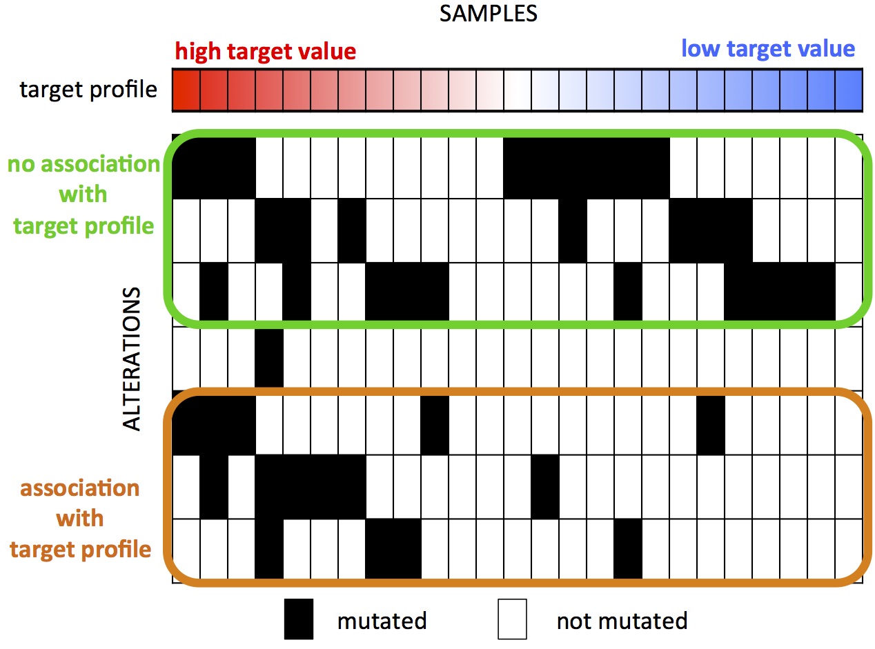
Fig 1: Identification of mutually exclusive alterations associated with a target profile.
Alterations in the green set have high mutual exclusivity but no association with the target profile. Alterations in the orange set have lower mutual exclusivity but strong association with the target profile. Methods that find mutually exclusive sets of alterations without considering the target profile will identify the green set as the most important gene set.

[33] recently developed the repeated evaluation of variables conditional entropy and redundancy (REVEALER) method, to identify mutually exclusive sets of alterations associated with functional phenotypes. REVEALER uses as objective function (to score a set of alterations) a re-scaled mutual information metric called information coefficient (IC). REVEALER employs a greedy strategy, computing at each iteration the conditional mutual information (CIC) of the target profile and each feature, conditioned on the current solution. REVEALER can be used to find sets of mutually exclusive alterations starting either from a user-defined seed for the solution or from scratch, and [33] shows that REVEALER finds sets of meaningful cancer-related alterations.

Our contribution

In this paper we study the problem of finding sets of alterations with complementary functional associations using alteration data and a quantitative (functional) target measure from a collection of cancer samples. Our contributions in this regard are fourfold. First, we provide a rigorous combinatorial formulation for the problem of finding groups of mutually exclusive alterations associated with a quantitative target and prove that the associated computational problem is NP-hard. Second, we develop two efficient algorithms, a greedy algorithm and an ILP-based algorithm to identify the set of $k$ genes with the highest association with a target; our algorithms are implemented in our method fUNctional Complementarity of alteratiOns discoVERy (UNCOVER). Third, we show that our algorithms identify highly significant sets of genes in various scenarios; in particular, we compare UNCOVER with REVEALER on the same datasets used in [33], showing that UNCOVER identifies solutions of higher quality than REVEALER while being on average two order of magnitudes faster than REVEALER. Interestingly, the solutions obtained by UNCOVER are better than the ones obtained by REVEALER even when evaluated using the objective function (IC score) optimized by REVEALER. Fourth, we show that the efficieny of UNCOVER enables the analysis of a large dataset from Project Achilles with thousands of target measurements and tens of thousands of alterations. On such dataset UNCOVER identifies identifies several statistically significant associations between target values and mutually exclusive alterations in genes sets sets, with an enrichment in well-known cancer genes and in known cancer pathways.

Materials and methods

This section describes the problem we study and the algorithms we designed to solve it, that are implemented in our tool UNCOVER. We also describe the data and computational environment for our experimental evaluation.

UNCOVER: Functional complementarity of alterations discovery

The workflow of our algorithm UNCOVER is presented in Fig. 2. UNCOVERtakes in input information regarding 1. the alterations measured in a number of samples (e.g., patients or cell lines), and 2. the value of the target measure for each patient. UNCOVER then identifies the set of mutually exclusive alterations with the highest association to the target, and employs a permutation test to assess the significance of the association. Details regarding the computational problem and the algorithms used by UNCOVER are described in the following sections. The implementation of UNCOVER is available at https://github.com/VandinLab/UNCOVER.

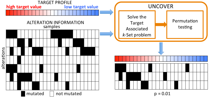
Fig 2: UNCOVER: Functional complementarity of alterations discovery.
UNCOVER takes in input the alterations information and a target profile for a set of samples, and identifies the set of complementary alterations with the highest association to the target by solving the Target Associated $k$-Set problem and performing a permutation test.

Computational problem

Let $J=\{j_{1},\dots,j_{m}\}$ be the set of samples and let $G=\{g_{1},\dots,g_{n}\}$ be the set of genes for which we have measured alterations in $J$. We are also given a target profile, that is for each sample $j\in J$ we have a target value $w_{j}\in\mathbb{R}$ which quantitatively measures a functional phenotype (e.g., pathway activation, drug response, etc.). For each sample $j\in J$ we also have information on whether each $g\in G$ is altered or not in $j$. Let $A_{g}$ be the set of patients in which gene $g\in G$ is mutated. We say that a patient $j\in J$ is covered by gene $g\in G$ if $j\in A_{g}$ i.e. if gene $g$ is mutated in sample $j$. Given a set of genes $S\subset G$, we say that sample $j\in J$ is covered by $S$ if $j\in\cup_{g\in S}A_{g}$.

The goal is to identify a set $S$ of at most $k$ genes, corresponding to $k$ subsets $S_{1},S_{2},\dots S_{k}$ where for each subset $S_{i}$ we have that $S_{i}\subseteq J$, such that the sum of the weights of the elements covered by $S$ is maximized. We also penalize overlaps between sets when an element is covered more than once by $S$ by assigning a penalty $p_{j}$ for each of the additional times $j$ is covered by $S$. As penalty we use the positive average of the normalized target values if the original weight of the element was positive. If the original weight of the element was negative we assign a penalty equal to its weight.

Let $c_{S}(j)$ be the number of sets in $S_{1},\dots,S_{k}$ that cover element $j\in J$.

Therefore for a set $S$ of genes, we define its weight $W(S)$ as:

$$W(S)=\sum_{j\in\cup_{s\in S}{A_{s}}}w_{j}-\sum_{j\in\cup_{s\in S}{A_{s}}}(c_{S}(j)-1)p_{j}$$

The Target Associated $k$-Set problem: missingGiven a set $J$ of samples, sets $A_{g_{1}},\dots,A_{g_{n}}$ describing alterations of genes $G=\{g_{1},\dots,g_{n}\}$ in the set $J$, weights $w_{j}$ and penalties $p_{j}>0$ for each sample $j\in J$ find the $S$ of $\leq k$ elements maximizing $W(S)$.

The following results defines the computational hardness of the problem above.

Theorem 1.

The Target Associated $k$-Set  problem is NP-hard.

Proof.

The proof is by reduction from the Maximum Weight Submatrix Problem (MWSP) defined and proved to be NP-hard in [34]. The MSWP takes as input an $m\times n$ binary matrix $A$ and an integer $k>0$ and requires to find the $m\times k$ column sub-matrix $\hat{M}$ of $A$ that maximizes the objective function $|\Gamma(M)|-\omega(M)$, where $\Gamma(M)$ is the set of rows with at least one $1$ in columns of $M$ and $\omega(M)=\sum_{g\in M}|\Gamma(\{g\})|-|\Gamma(M)|$.

Given an instance of Maximum Weight Submatrix Problem, we define an instance of the Target Associated $k$-Set as follow: the set of samples $J$ corresponds to the rows of $A$, the set of genes $G$ corresponds to the columns of $A$, and the set $S_{g}$ of samples covered by gene $g\in G$ is the subset of the rows in which $g$ has a 1. By setting $w_{j}=1$ and $p_{j}=1$ for all $j\in J$, we have that the objective function of MWSP corresponds to the weight $W(S)$ for the Target Associated $k$-Set  therefore the optimal solution of the Target Associated $k$-Set corresponds to the optimal solution of MWSP. ∎

ILP formulation

In this subsection we provide an ILP formulation for the Target Associated $k$-Set problem. Let $x_{i}$ be a binary variable equal to $1$ if set $i\in G$ is selected and $x_{i}=0$ otherwise. Let $z_{j}$ be a binary variable equal to $1$ if element $j$ is covered and $z_{j}=0$ otherwise. Let $y_{j}$ denote the number of sets in the solution covering element $j$. Finally, let $w_{j}$ be the weight of element $j$ and $p_{j}$ be the penalty for element $j$

In our ILP formulation, the following constraints need to be satisfied by a valid solution:

• the total number of sets in the solution is at most $k$: $\sum_{i}x_{i}\leq k$

• for each element $j\in J$ we have: $y_{j}=\sum_{i:j\in S_{i}}x_{i}$

• for each element $j\in J$, if $j$ is covered by the current solution then the number of times $j$ is covered in the solution is at least $1$: $y_{j}\geq z_{j}$

• for each element $j\in J$, if $j$ is covered by at least one element in the current solution then $j$ is covered: $z_{j}\geq y_{j}/k$.

With the variables defined above, the score for a given solution is

$$z(q)=\max\sum_{j=1}^{m}(w_{j}+p_{j})z_{j}-\sum_{j=1}^{m}p_{j}y_{j}.$$ (1)

$z(q)$ constitutes the objective function of our ILP formulation.

Greedy algorithm

Since solving ILPs can be impractical for very large datasets, we also design a $k$-stage greedy algorithm to solve the Target Associated $k$-Set problem. During each stage the algorithm picks 1 set $A_{i}$ to be part of the solution; this is done by first computing the total weight of each subset which is defined as the sum of the weights of its elements $W(A_{i})=\sum_{j\in A_{i}}w_{j}$. Then the algorithm finds the subset $A_{i}$ of maximum positive weight and adds it to the solution. It may be that at some stage $\ell$ no additional set of positive weight can be selected, in this case, the solution obtained after stage $\ell-1$ will be our output. At the end of the iteration the weight of every element $j$ that belonged to the chosen set $A_{i}$ is set to the negative of penalty $p_{j}$, in order to penalize future selections of the same elements. The greedy algorithm is described in Algorithm 1.

Input: A set of elements $J$ (samples), a class $I$ of subsets of $J$ (genetic alterations) and an integer $k$ (number of alterations we want to find). Each element $j\in J$ has an associated weight $w_{j}$ (target profile) and a penalty $p_{j}$.

Output: $k$ subsets, $S_{1},S_{2},\dots S_{k}$ , where each subset selected is a member of $I$, such that the sum of the weights of the elements in the selected sets is maximized and the overlap between selected sets is minimized.

for $\ell\leftarrow 1$ to $k$ do

       for $i\leftarrow 1$ to $n$ do $W(A_{i})\leftarrow\sum_{j\in A_{i}}w_{j}$;

       $S_{\ell}\leftarrow\arg\max_{A_{i}>0}\{W(A_{i})\}$;

       for $j\in S_{\ell}$ do $w_{j}\leftarrow-p_{j}$;

      

end for

return $S_{1}\dots S_{k}$;

Algorithm 1 Greedy Coverage

We note that our greedy algorithm is analogous to the greedy algorithm for the Maximum k-Coverage problem [35] with the difference that rather than eliminating the elements already selected we change their weight to a penalty. Also, assuming it is acceptable to return less than $k$ sets, we only pick a set if it has a positive weight. The running time of the algorithm is $O(kmn)$ where $m=$ number of samples and $n=$ number of alterations.

While the greedy algorithm may not return the optimal solution, we prove that it provides guarantees on the weight of the solution it provides.

Proposition 1.

Let $S^{*}$ the optimal solution of the Target Associated $k$-Set and $\hat{S}$ be the solution returned by the greedy algorithm. Then $W(\hat{S})\geq W(S^{*})/k$.

Proof.

Note that the weight of subsets in the optimal solution $W(S^{*})$ can only be lower compared to the original weight of the subsets, since the only weight update operation performed is to substitute positive weights of elements selected with a negative penalty.

The first subset $\hat{S_{1}}$ selected by our algorithm is the set of maximum weight out of all subsets and therefore $W(\hat{S_{1}})\geq W(S_{\ell}^{*})$ for $\ell=1..k$. By the pigeonhole principle, one of these subsets in the optimal solution must cover at least $W(S^{*})/k$ worth of elements. Thus $W(\hat{S_{1}})\geq W(S^{*})/k$. Therefore the first subset selected by the algorithm already gives a $1/k$ approximation of the optimal solution. In subsequent iterations of the algorithm we only pick additional sets if they have a positive weight so our approximation ratio can only improve. ∎

We also prove that the bound above is tight

Proposition 2.

There are instances of the Target Associated $k$-Set such that $W(\hat{S})=W(S^{*})/k$.

The proof is in the Supplementary Material.

While the proposition above is based on an extreme example, our experimental analysis shows that in practice the greedy algorithm works well and often identifies the optimal solution. We therefore analyze the greedy algorithm under a generative model in which there is a set $H$ of $k$ genes with mutually exclusive alterations associated with the target, while each genes $g\in G\setminus H$ is mutated in sample $j$ with probability $p_{g}$ independently of all other events. We also assume that the weights $w_{j}$ are such that $\sum_{j\in J}w_{j}=0$ and for each $j:|w_{j}\leq 1|$. (In practice this is achieved by normalizing the target values before running the algorithm, by subtracting to each $w_{j}$ the average value $\sum_{j\in J}w_{j}/m$ and then dividing the result by the maximum of the absolute values of the transformed $w_{j}$’s.) Note that this last condition implies that $|p_{j}|\leq 1$ for all $j$. We also assume that for genes in $H$ the following assumptions hold:

• the set $H$ has an association with the target, i.e.: $\mathbf{E}[W(H)]\geq\frac{m}{c^{\prime}}$ for a constant $c^{\prime}\geq 1$.

• each gene of $H$ contributes to the weight of $H$, i.e. for each $S\subset H$ and each $g\in H\setminus S$ we have $\mathbf{E}[W(S\cup\{g\})]-\mathbf{E}[W(S)]\geq\frac{W(H)}{kc^{{}^{\prime\prime}}}$ for a constant $c^{{}^{\prime\prime}}\geq 1$.

The following shows that, if enough samples from the generative model are considered, the greedy algorithm finds the set $H$ associated with the target with high probability.

Proposition 3.

If $m\in{\Omega}\left(k^{2}\ln(n/\delta)\right)$ samples from the generative model above are provided to the greedy algorithm, then the solution of the greedy algorithm is H with probability $\geq\delta$.

The proof is in the Supplementary Material.

Statistical significance

To assess the significance of the solution reported by our algorithms we use a permutation test in which the dependencies among alterations in various genes are maintained, while the association of alterations and the target is removed. In particular, a permuted dataset under the null distribution is obtained as follows: the sets $A_{g},g\in\mathcal{G}$ are the same as observed in the data; the values of the target are randomly permuted across the samples.

To estimate the $p$-value for the solutions obtained by our methods we used the following standard procedure: 1) we run an algorithm (ILP or greedy) on the real data $\mathcal{D}$, obtaining a solution with objective function $o_{\mathcal{D}}$; 2) we generate $N$ permuted datasets as described above; 3) we run the same algorithm on each permuted dataset; 4) the $p$-value is the given by $(e+1)/(N+1)$, where $e$ is the number of permuted datasets in which our algorithm found a solution with objective function $\geq o_{\mathcal{D}}$.

Data and computational environment

Alteration Data.

We downloaded data for the Cancer Cell Line Encyclopedia on $25^{th}$ September, 2017 from http://www.broadinstitute.org/ccle. In particular we used the mutation (single nucleotide variants) and copy number aberrations (CNAs) which are derived from the original Cancer Cell Line Encyclopedia (CCLE) mutations and CNA datasets. The file we used is CCLE_MUT_CNA_AMP_DEL_0.70_2fold.MC.gct. It consists of a binary (0/1) matrix across 1,030 samples and 48,270 gene alterations in the form of mutations, amplifications and deletions, with a 1 meaning that the alteration is present in a sample, and a 0 otherwise.

Target Data.

In terms of target values we use the same datasets used by [33] to compare the performance of UNCOVER with REVEALER. In particular we used the following files available through the Supplementary Material of [33]: CTNBB1_transcriptional _reporter.gct, which consists of measurements of a $\beta$-catenin reporter in 81 cell lines; NFE2L2_activation_profile.gct, which includes NFE2L2 enrichment profiles for 182 lung cell lines; MEK_inhibitor_profile.gct, which contains MEK-inhibitor PD-0325901 sensitivity profile in 493 cancer cell lines from the Broad Novartis CCLE14l; and KRAS_essentiality_profile.gct, which corresponds to the feature KRAS from a subset of 100 cell lines from the Achilles project dataset. In all these cases we considered the same direction of association (positive or negative) between alterations and the target as in [33]. Since our algorithm is very efficient we then decided to run it on a large dataset from Project Achilles  (https://portals.broadinstitute.org/achilles), that uses genome-scale RNAi and CRISPR-Cas9 perturbations to silence or knockout individual genes. In particular, we use the whole 2.4.2 Achilles dataset (Achilles_QC_v2.4.3.rnai.Gs.gct) available from the project website. This dataset provides phenotype values for 5711 targets, corresponding to genes silenced by shRNA. The phenotype values correspond to ATARiS [37] gene (target) level scores, quantifying the cell viability when the target gene is silenced by shRNA. These scores are provided for 216 cell lines [19], with 205 of them appearing in CCLE.

Data Preprocessing.

To be consistent with REVEALER we discarded features with high or low frequency, in particular features present in less than 3 samples or more than 50 samples were excluded from our analyses. The only exception was the MEK-inhibitor example, where the high frequency threshold was changed to be 100 since the number of original samples was substantially higher (i.e., 493) for this case. From the Achilles dataset we excluded targets that have at least one missing value, in particular in this case we exclude 21 of the 5711 sets of target scores. In all our experiments we normalized the target values before running the algorithm, by subtracting to each weight $w_{j}$ the average value $\sum_{j\in J}w_{j}/m$ and dividing the result by the standard deviation of the (original) $w_{j}$’s, in order to have both positive and negative target values.

Simulated Data.

We investigated how effective UNCOVER is at finding selected alterations in a controlled setting, where the ground truth is known. We generated target values according to a normal distribution with mean 0 and standard deviation 1. We tested dataset with 200, 600, 1000 and 10000 samples. For each dataset we considered the 38002 gene alterations present in CCLE and for each of them we placed alterations in the samples independently of all other events with the same frequencies as they appear in CCLE. To be consistent with the preprocessing done on rel data we filtered alterations to only have alterations with frequencies between 0.1 and 0.25. We also generated a set $T$ of 5 features to have an association with the target values. This association was varied throughout the experiments to cover different percentages of positive and negative targets. In particular we generated the selected features to cover 100%, 80%, 60%, 40% of the positive target values and 5%, 10%, 15%, 20% of the negative target values respectively, chosing random subsets of samples with positive or negative target values. We will refer to the parameter indicating the percentage of samples with positive target values selected as $P$ and to the parameter for the percentage of samples with negative target values selected as $N$. We divided the number of targets covered by each of the 5 mutations equally.

Computing Environment and Solver Configuration.

To describe and solve an ILP we used AMPL 20150516 and CPLEX 12.6.3. All parameters in CPLEX were left at their default values. We implemented our greedy algorithm in Python 3.6.1. We run our experiments (with the exception of experiments conducted on simulated data) on a MacBook Air with 1.7 GHz Intel Core i7 processor, 8 GB RAM and 500 GB of local storage. In order to make a time comparison with REVEALER we also run the R code provided in [33] on the same machine, using R 3.3.3. All the parameters were left at their given values except for the number of permutations used to calculate their p-value, which we changed in order to compare the running time of the methods excluding the time needed to compute $p$-values. Experiments on simulated data were conducted on local nodes of a computing cluster. Each node had the following configuration: four 2.27 GHz CPUs, 5.71 GB RAM and 241 GB of storage.

Results and discussion

We tested UNCOVER on a number of cancer datasets in order to compare its results with state-of-the-art algorithms and to test whether UNCOVER allows the analysis of large datasets. In particular we used four datasets described in [33] to compare UNCOVER with REVEALER, and then performed a large scale analysis using targets from the Achilles project dataset and alterations from the Cancer Cell Line Encyclopedia (CCLE).

Comparison with REVEALER

We run the greedy algorithm and the ILP from UNCOVER on the same four datasets considered by the REVEALER publication [33]. We used the same values of $k$ used in [33], that is $k=3$ for all the datasets, except from the KRAS dataset where $k=4$ was used. For each dataset we recorded the solution reported by the greedy algorithm, the solution reported by the ILP, the value of the objective functions for such solutions and the running time to obtain such solutions. For ILP solutions, we also performed the permutation test (see Materials and methods) to compute a $p$-value using $1000$ permutations. The results are reported in Table 1, in which we also show the results from REVEALER (without initial seeds). Fig. 3 shows alteration matrices and the association with the target for the solutions identified by UNCOVER.

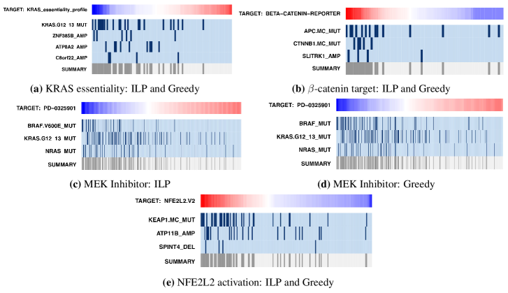
Fig 3: Results of UNCOVER on four cancer datasets from [33].
(a) Solution found by ILP and greedy for KRAS essentiality target. (b) Solution found by ILP and greedy for $\beta$-catenin activation target. (c) Solution found by ILP for MEK inihibitor target. (d) Solution found by greedy for MEK inihibitor target. (e) Solution found by ILP and greedy for NFE2L2 activation target. Each panel shows the value of the target (top row) for various samples (columns), with red being positive and blue being negative values. For each gene in the solution, alterations in each sample are shown in dark blue, while samples not altered are in light blue. The last row shows the alteration profile of the entire solution.

We can see that the greedy algorithm identifies the same solution of the ILP based algorithm in three out of four cases, and that the runtime of the ILP and the runtime of greedy algorithm are comparable and very low ($<40$ seconds) in all cases. In contrast, the running time of REVEALER is much higher ($>1000$ seconds in most cases). (We included all preprocessing in the reported runtimes in table 1 to ensure a fair comparison with REVEALER; not including preprocessing our running times are all under 10 seconds.) Comparing the alteration matrices of the solutions by UNCOVER and the ones of solutions by REVEALER (Supplementary Fig. 7) we note that alterations in solutions by UNCOVER tend to have higher mutual exclusivity and to be more concentrated in high weight samples than alterations in solutions by REVEALER. As expected, the value of the objective function we use is much lower for solutions from REVEALER than for solutions from our algorithm.

Table 1: Comparison of our algorithms with REVEALER.

	NFE2L2 activation	MEK-inhibitor	KRAS essentiality	$\beta$-catenin activation
ILP solution	KEAP1.MC MUT	BRAF.V600E MUT	KRAS.G12 13 MUT	APC.MC MUT
	ATP11B AMP	KRAS.G12 13 MUT	ZNF385B AMP	CTNNB1.MC MUT
	SPINT4 DEL	NRAS MUT	ATP8A2 AMP	SLITRK1 AMP
			C8orf22 AMP
Objective value	46.17	108.32	28.00	22.97
IC score	0.58	0.49	0.63	0.67
p-value	0.000999	0.000999	0.025974	0.1068931
Running time (s)	14	39	9	9
Greedy solution	KEAP1.MC MUT	BRAF MUT	KRAS.G12 13 MUT	APC.MC MUT
	ATP11B AMP	KRAS.G12 13 MUT	ZNF385B AMP	CTNNB1.MC MUT
	SPINT4 DEL	NRAS MUT	ATP8A2 AMP	SLITRK1 AMP
			C8orf22 AMP
Objective value	46.17	104.29	28.00	22.97
IC score	0.58	0.5	0.63	0.67
Running time (s)	15	35	9	8
REVEALER solution	KEAP1.MC MUT	BRAF MUT	KRAS.G12 13 MUT	APC.MC MUT
	LRP1B DEL	KRAS.G12 13 MUT	ZNF385B AMP	CTNNB1.MC MUT
	OR4F13P AMP	NRAS MUT	LINC00340 DEL	ITGBL1 AMP
			NUP153 MUT
Objective value	30.35	104.29	21.86	22.12
IC score	0.54	0.5	0.6	0.7
Running time (s)	1615	4965	1243	787

For each of the four targets (NFE2L2 activation, MEK-inhibitor, KRAS essentiality, $\beta$-catenin activation) considered in [33], the set of alterations of cardinality $k$ reported by our ILP algorithm, by our greedy algorithm, and by REVEALER (without seeds) is reported. $k$ is chosen as in [33]. For each pair (algorithm, target) we also report the (objective) value of our objective function for the solution, the value of the IC score (that is, the objective function used in [33]), and the running time of the algorithm for the target. For solutions found by our ILP we also report the $p$-value computed by permutation test using 1000 permutations.

We then compared the solutions obtained by our algorihtms with the solutions from REVEALER in terms of the information coefficient (IC), that is the target association score used in [33] as a quality of the solution. Surprisingly, in two out of four datasets UNCOVER, which does not consider the IC score, identifies solutions with IC score higher (by at least $5\%$) than the solutions reported by REVEALER. For the other two cases, in one dataset the IC score is very similar (0.50 vs 0.49) while in the other case the IC score by REVEALER is higher (0.7 vs 0.67) but the solution reported by REVEALER differs from the solution reported by UNCOVER by 1 gene only. Interestingly, the latter is the only case where the solution from the ILP has a $p$-value $>0.1$ ($p<0.03$ in all other cases), and therefore the solutions (by our methods and by REVEALER) for such dataset may be, at least in part, due to random fluctuations of the data.

In most cases the solutions by UNCOVER and by REVEALER are very similar, with cancer relevant genes identified by both methods. For NFE2L2 activation, both methods identify KEAP1, a repressor of NFE2L2 activation [38]. For MEK-inhibitor, both methods find BRAF, KRAS, and NRAS, three well knwon oncogenic activators of the MAPK signaling pathway, which contains MEK as well. For KRAS essentiality, both methods report mutations in KRAS in the solution. For $\beta$-catenin activation, both methods identify CTNNB1 mutations and APC mutations, that is known to be associated to $\beta$-catenin activation [39]. These results show that UNCOVER identifies relevant biological solutions that are better than the ones identified by REVEALER when evaluated using our objective function and also when evaluated according to the objective function of REVEALER with a running time that is on average two orders of magnitude smaller than required by REVEALER.

Results on simulated data

For each combination we generated 10 simulated dateset as described in Materials and methods. Each dataset contains a planted set of 5 alterations associated with the target. We used both the greedy algorithm and the ILP from UNCOVER  with $k=5$ to attempt to find the 5 correct alteration, and evaluated our algorithms both in terms of fraction of the correct (i.e., planted) solution reported and running time.

As shown in Fig. 4, the greedy algorithm is faster than the ILP for all datasets, and the difference in running time increases as the number $m$ of samples increases, with the runtime of the greedy algorithm being almost two order of magnitude smalle than the runtime of the ILP for $m=1000$ samples. In addition, for a fixed number of samples and alterations, the running time of the greedy algorithm is constant, that is it does not depend on the properties of the planted solution, while the running time of the ILP varies greatly depending on these parameters. For $m=10,000$ samples the running time of the ILP becomes extremely high, so we restricted to consider only two sets of paramters ($p-n=0.95$ and $p-n=0.2$). In this case the ILP took between 44 minutes and 7 hours to complete, while the greedy algorithm terminates in 5 minutes.

In terms of the quality of the solutions found, as expected the ILP outperforms the greedy (Fig. 5) but the difference among the two tends to disappear when the number of samples is higher. In addition, since the ILP finds the optimal solution, we can see that for a limited number of samples we may not reliably identify the planted solution with 200 samples unless the planted solution appears almost only in positive targets and in almost all of them ($p-n=0.95$), while for m=$1000$ we can reliably identify the planted solution using both the ILP and the greedy algorithm even when the association with the target is weaker ($p-n=0.6)$. When $m=10,000$, both the ILP and the greedy algorithm perform well in terms of the quality of the solution: the ILP finds the correct alterations on every experiment and the greedy identifies the whole planted solution in all experiments but one for $p-n=0.2$, for which it still reports a solution containing 4 genes in the planted solution.

These results show that for a large number of samples the greedy algorithm reliably identifies sets of alterations associated with the target, as predicted by our theoretical analysis, and is much faster than the ILP. For smaller sample size the ILP identifies better solutions than the greedy and has a reasonable running time.

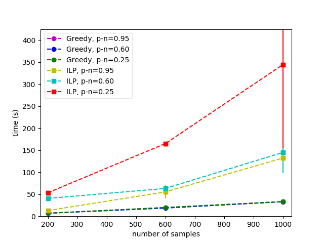
Fig 4: Running time of UNCOVERon simulated data.
The running time (expectation and standard deviation) of the greedy algorithm and of the ILP approach are shown for different number of samples and the difference $p-n$ between the percentage $p$ of samples with positive target and the percentage $n$ of samples with negative target covered by the the correct solution.

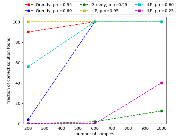
Fig 5: Quality of solutions of UNCOVERon simulated data.
The fraction of genes in the planted (i.e., correct) solution found by the greedy algorithm and by the ILP approach are shown for different number of samples and the difference $p-n$ between the percentage $p$ of samples with positive target and the percentage $n$ of samples with negative target covered by the the correct solution.

Analysis of Achilles project data

The efficiency of UNCOVER renders the analysis of a large number of targets, such as the ones available through the Achilles project, possible. After preprocessing the dataset included 5690 functional phenotypes as targets, and for each of these the CCLE provides alteration information for 205 samples and 31137 alterations. In total we have therefore run 10380 instances (i.e., 5690 targets screened for positive and for negative associations) looking for both positive and negative association with target values. Since the number of samples (205) is relatively small, we have run only the ILP from UNCOVER on the whole Achilles dataset and looked for solutions with $k=3$ genes. The runtime of UNCOVER to find both positive and negative associations, including preprocessing, is 24 hours. Based on the runtime required on the instances reported in [33] (see the Comparison with REVEALER section), running REVEALER on this dataset would have required about 5 months of compute time.

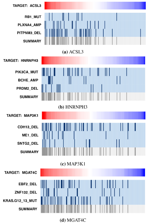
Fig 8: Alteration matrices for results of UNCOVER the Achilles Project data.

To identify statistically significant associations with targets in the Achilles project dataset we used a nested permutation test. We first run the permutation test with 10 permutations on all instances (i.e., on all targets for both positive association and negative association). We then considered all the instances with the lowest p-value (1/11) and performed a permutation test with 100 permutations only for such instances. We the iterated such procedure once more, selecting all the instances with lowest p-value (1/101) and performing a permutation test with 1000 permutations only for such instances. For positive association we found 60 solutions with $p$-value $<0.001$, and for negative association we found 102 solutions with $p$-value $<0.001$. The solutions with $p$-value $<0.001$ (with 1000 permutations) are reported in Supplementary Table 2 and  3. See Supplemental Fig. 8 for some corresponding alteration matrices.

The genes in the solutions by UNCOVER with p-value $1/1001$ are enriched ($p=2\times 10^{-12}$ by Fisher exact test) for well-known cancer genes, as reported in [11]. We also tested whether genes in solutions by UNCOVER (with p-value $1/1001$) are enriched for interactions, by comparing the number of interactions in iRefIndex [40] among genes in such solution with the number of interactions in random sets of genes of the same cardinality. Genes in solutions by UNCOVER are significantly enriched in interactions ($p=7\times 10^{-3}$ by permutation test). In addition, the genes in solutions by UNCOVER are also enriched in genes in well-known pathways: 12 KEGG pathways [41] have a significant (corrected $p\leq 0.05$) overlap with genes in solutions by UNCOVER and four of these (endometrial cancer, glioma, hepatocellular carcinoma, EGFR tyrosine kinase inhibitor resistance) are cancer related pathways. In addition, the targets (i.e., genes) with solutions of $p$-value $1/1001$ are enriched ($p=10^{-3}$ by permutation test) for interactions in iRefIndex and for well-known cancer genes as reported in [11]. These results show that UNCOVER enables the identification of groups of well known cancer genes with significant associations to important targets in large datasets of functional target profiles. For example, for target (i.e., silenced gene) TSG101, related to cell growth, UNCOVER identifies the gene set shown in Figure 6 as associated to reduced cell viability. ERBB2 is a well known cancer gene and CDH4 is frequently mutated in several cancer types, and both are associated to cell growth.

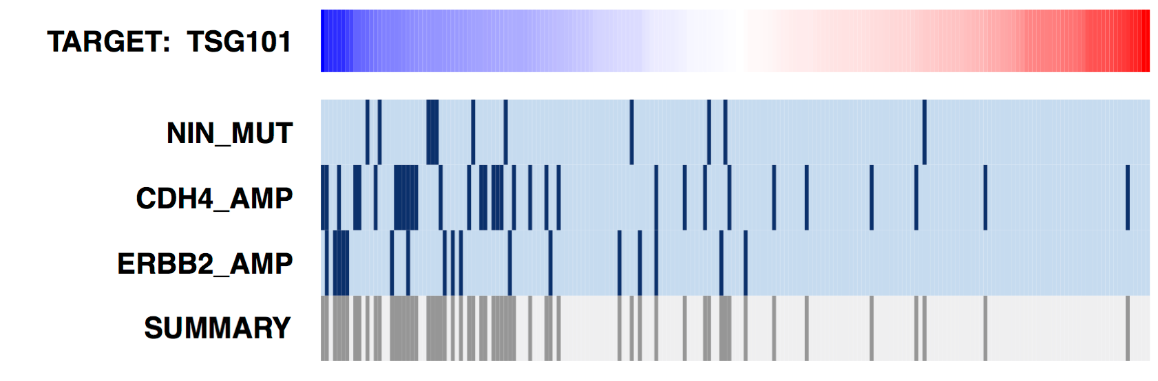
Fig 6: Solution by UNCOVER for silencing of TSG101 (data from Achilles Project).
The alteration matrix of genes in the solution identified by UNCOVER as associated to reduced cell viability is reported. The figure shows the value of the target (top row) for various samples (columns), with blue being negative values (i.e., reduced cell viability) and red being positive values. For each gene in the solution, alterations in each sample are shown in dark blue, while samples not altered are in light blue. The last row shows the alteration profile of the entire solution.

Conclusion

In this work we study the problem of identifying sets of mutually exclusive alterations associated with a quantitative target profile. We provide a combinatorial formulation for the problem, proving that the corresponding computational problem is NP-hard. We design two efficient algorithms, a greedy algorithm and an ILP-based algorithm, for the identification of sets of mutually exclusive alterations associated with a target profile. We provide a formal analysis for our greedy algorithm, proving that it returns solutions with rigorous guarantees in the worst-case as well under a reasonable genarative model for the data. We implemented our algorithms in our method UNCOVER, and showed that it finds sets of alterations with a significant association with target profiles in a variety of scenarios. By comparing the results of UNCOVER with the results of REVEALER on four target profiles used in the REVEALER publication [33], we show that UNCOVER identifies better solutions than REVEALER, even when evaluated using REVEALER objective function. Moreover, UNCOVER is much faster than REVEALER, allowing the analysis of large datasets such as the dataset from project Achilles, in which UNCOVER identifies a number of associations between functional target profiles and gene set alterations. Our tool UNCOVER (as well as REVELEAR) relies on the assumption that the mutual exclusivity among alterations is due to functional complementarity. Another explanation for mutual exclusivity is the fact that each cancer may comprise different subtypes, with different subtypes being characterized by different alterations [27]. UNCOVER can be used to identify sets of mutually exclusive alterations associated with a specific subtype whenever the subtype information is available, by assigning high weight to samples of the subtype of interest and low weight to samples of the other subtypes.

Supplementary Material

Proposition 4.

There are instances of the Target Associated $k$-Set such that $W(\hat{S})=W(S^{*})/k$.

Proof.

To see that the bound is tight just consider the following example. We want to pick k sets out of n sets $A_{1}...A_{n}$. Sets $A_{1}...A_{k}$ include 2 elements of respective weight $a\geq 0$ and $b=a/(k-1)$. Subset $A_{k+1}$ includes all the elements of weight $b$ from the previous $k$ sets and one element with a small weight $\epsilon$. Each of the remaining sets $A_{k+2}...A_{n}$ include an arbitrary number of elements with overall weight $\leq 0$. We choose a penalty of value $a$. Note that one can choose the weights of elements in sets $A_{k+2}...A_{n}$ in such a way that the average of all positive normalized weights is equal to $a$. Clearly the optimal solution to the Target Associated $k$-Set problem consists of sets $A_{1}...A_{k}$ with an objective value of $k(a+b)$. The greedy algorithm will pick set $A_{k+1}$ at the first iteration and then assign a new weight to its elements equal to $-a$. The updated weight of sets $A_{1}...A_{k}$ is now 0 and the algorithm will stop and output $A_{k+1}$ as the solution, giving an approximation ratio of

$$\frac{kb+\epsilon}{k(a+b)}=\frac{1}{k}+\frac{\epsilon}{kb}$$

∎

Proposition 5.

If $m\in{\Omega}\left(k^{2}\ln(n/\delta)\right)$ samples from the generative model above are provided to the greedy algorithm, then the solution of the greedy algorithm is H with probability $\geq\delta$.

Proof.

We prove that in iteration $i$ of the greedy algorithm, conditioning on the current solution being a set $S$ with $S\subset H$, then the greedy algorithm adds a gene in $H\setminus S$ to the solution with probability $\geq delta/k$, and that the first gene added by the greedy algorithm is $g\in H$. The result then follows by union bound on the $k$ iterations of the greedy algorithm.

Consider the first iteration of the greedy algorithm and consider a gene $g\in G$. Note that if $g\not\in H$ then $\mathbf{E}[W(\{g\})]\leq 0$, since $\mathbf{E}[\sum_{j\in A_{g}}w_{j}]=0$ because the samples in which $g$ is mutated are taken uniformly at random while $\sum_{j\in A_{g}}(c_{S}(j)-1)\geq 0$. If $g\in H$ by the assumptions of the model we have $\mathbf{E}[W(\{g\})]\geq\frac{m}{kc^{{}^{\prime\prime\prime}}}$ for a constant $c^{\prime\prime\prime}\geq 1$. Note that $W(\{g\})$ can be written as the sum $\sum_{i=1}^{m}X_{i}$ of random variables (r.v.’s) $X_{i}$ where $X_{i}$ is the contribution of sample $i$ to $W(\{g\})$ with $X_{i}\in[-1,1]$. By the Azuma-Hoeffding inequality [36] and union bound (on the $n$ genes) the first gene chosen by the greedy algorithm is not gene $g\in H$ with probability $\leq e^{-\frac{2m^{2}}{4mk^{2}(c^{{}^{\prime\prime\prime}})^{2}}}$ which is $\leq\delta/k$ when $m\in{\Omega}\left(k^{2}\ln(nk/\delta))\right)$.

Now assume that in iteration $i$, for the current solution $S\subset H$. Consider a gene $g\in G\setminus H$, then $\mathbf{E}[W(S\cup\{g\})-W(S)]\leq 0$, since $\mathbf{E}[\sum_{j\in\cup_{s\in S\cup{g}}{A_{s}}}w_{j}-\sum_{j\in\cup_{s\in S}{A_{s}}}w_{j}]\leq 0$ (by the assumptions of the model $W(S)>0$ and the fact that alterations in $\{g\}$ are placed uniformly at random among samples) and $\mathbf{E}[\sum_{j\in\cup_{s\in S\cup{g}}}(c_{S}(j)-1)-\sum_{j\in\cup_{s\in S}}(c_{S}(j)-1)]\geq 0$ (because for each sample $i$, the number of alterations of $S\cup\{g\}$ in $i$ is a superset of the number of alterations of $S$ in $i$). Consider now a gene $g\in H\setminus S$: by the assumptions of the model $\mathbf{E}[W(S\cup\{g\})-W(S)]\leq\frac{m}{kc^{{}^{\prime\prime\prime}}}$ for a constant $c^{{}^{\prime\prime\prime}}>1$. Note that $\mathbf{E}[W(S\cup\{g\})-W(S)$ can be written as the sum of $\sum_{i=1}^{m}X_{i}$ of random variables (r.v.’s) $X_{i}$ where $X_{i}$ is the contribution of sample $i$ in the increase in weight from $W(S)$ to $W(S\cup\{g\})$, where $X_{i}\in[-1,1]$. By the Azuma-Hoeffding inequality and union bound (on the $<n$ genes considered for addition by the greedy algorithm) the gene $g$ added to $S$ by the greedy algorithm in iteration $i$ is not in $H\setminus S$ with probability $\leq e^{-\frac{2m^{2}}{4mk^{2}(c^{{}^{\prime\prime\prime}})^{2}}}$ which is $\leq\delta/k$ when $m\in{\Omega}\left(k^{2}\ln(nk/\delta))\right)$. ∎

Table 2: Solutions found when running our ILP algorithm for the Achilles dataset, looking for positive correlation with the target. For each target we report the objective function value for the optimal solution, the set of alterations of cardinality 3 and the p-value computed by permutation test using 1000 permutations

target	objective	alterations:
VAMP7	50.19	CLYBL_AMP	FBXL17_DEL	ARHGEF10_DEL
VHLL	43.87	ZNF705B_DEL	FARS2_DEL	ZRANB2_DEL
TRIM13	43.75	AMY2A_AMP	SH3KBP1_DEL	LOC649352_DEL
QDPR	43.39	DAB1_MUT	SLX1A_DEL	RPL23AP53_DEL
CD302	43.36	FRG2C_DEL	LOC650623_DEL	CTDP1_DEL
DDX4	43.23	LYPD8_AMP	TRIM28_AMP	SLC18A1_DEL
ZNF439	43.21	PLCXD3_AMP	ITGA7_AMP	PMP22_DEL
PTBP3	42.58	TAOK3_MUT	MRPS30_AMP	ALOX15_DEL
SRGAP3	42.42	FAM66B_AMP	SCAND3_AMP	C17orf101_AMP
C10orf10	42.12	HLA-A_DEL	CDH12_AMP	PTPRT_DEL
TNIP1	42.10	LINC00547_AMP	XG_AMP	LOC729732_DEL
PAWR	42.02	EPSTI1_AMP	GPLD1_DEL	DLGAP2_DEL
PRDM5	41.99	ADAD2_DEL	HSD17B10_DEL	IMMP2L_DEL
TXNDC5	41.90	MEP1B_DEL	SFRP1_DEL	ZNF385D_DEL
TXNDC5	41.90	MEP1B_DEL	SFRP1_DEL	ZNF385D_DEL
ACSL3	41.85	RB1_MUT	PLXNA4_AMP	PITPNM3_DEL
ANAPC2	41.78	HERC2P3_DEL	LCE1D_AMP	MAP1LC3A_AMP
CNDP2	41.76	EPSTI1_AMP	PITPNA_DEL	FAM86B2_DEL
MDM4	41.75	LY86-AS1_DEL	THSD7B_AMP	LINC00583_DEL
ADCYAP1R1	41.69	HEATR4_AMP	EPB41L4A_DEL	DLGAP2_DEL
NMBR	41.64	LOC100506136_AMP	AP4S1_AMP	PSPC1_DEL
PPP2R2D	41.64	LZTS1_DEL	NF1P2_DEL	QKI_DEL
SLC39A10	41.64	OBSCN_MUT	LOC100302640_AMP	SGSM2_DEL
GK	41.61	DST_MUT	ADCY8_DEL	ARHGAP44_DEL
EIF4E	41.36	GUSBP9_AMP	PON2_AMP	CAB39L_DEL
SLC31A1	41.26	FAM66E_DEL	TMEM132C_DEL	CD83_DEL
PLS3	41.24	LOC154872_AMP	FAM60A_AMP	KRT16P2_DEL
CCT5	41.20	RASA4_DEL	GUSBP1_AMP	KCNQ5_DEL
FFAR2	41.17	PTPRT_DEL	ERICH1_DEL	NBEAP1_DEL
OR4K17	41.15	THSD7B_AMP	C6orf201_DEL	FAM86B2_DEL
TCEB1	41.09	DENND5B_AMP	SLC1A3_AMP	SLIT3_DEL
FGD1	41.08	MLL3_MUT	MIR19B1_AMP	MSR1_DEL
HNRNPH3	40.99	PIK3CA_MUT	BCHE_AMP	PRDM2_DEL
EFHB	40.93	FANCM_MUT	WDR7_DEL	RIMS2_DEL
MIF	40.90	FRG2C_DEL	LINC00340_DEL	PPP3CC_DEL
PRKY	40.85	ATP11A_MUT	TCEB3C_DEL	NFIB_DEL
MGAT4C	40.81	EBF2_DEL	ZNF132_DEL	KRAS.G12_13_MUT
RCN2	40.54	MYLK_MUT	PIK3C2G_MUT	FAM86B1_DEL
CSE1L	40.49	LY86-AS1_DEL	COL1A2_AMP	GLIPR2_DEL
DGKG	40.23	MEP1B_DEL	PARD3B_DEL	MEX3C_DEL
MST1R	40.20	SLC6A10P_DEL	GOLPH3L_AMP	OR52N5_DEL
TLR4	39.91	C18orf61_AMP	PTEN_DEL	LOC728875_DEL
OR4D11	39.85	CREBBP_MUT	MIR4796_AMP	LOC340357_DEL
CD47	39.71	STK3_AMP	LOC728190_AMP	NLRP1_DEL
RNF183	39.71	GPR112_MUT	IFLTD1_AMP	LOC340357_DEL
SULT1A3	39.68	LY86-AS1_DEL	CACNA1D_DEL	SEC24D_DEL
SULT1A4	39.68	LY86-AS1_DEL	CACNA1D_DEL	SEC24D_DEL
FGG	39.66	H3F3C_AMP	MSRA_DEL	PSG5_DEL
NFAT5	39.40	LOC286184_AMP	PCTP_AMP	MIR4744_DEL
ANKRD5	39.40	COL14A1_AMP	CXADRP2_DEL	OPALIN_DEL
MGP	39.37	TFAP2D_AMP	GAL_AMP	LOC728323_DEL
PDE12	39.32	HTR3C_AMP	GALNTL2_DEL	APC.MC_MUT
RAB31	39.31	IGLL5_AMP	FAM106CP_DEL	PACRG_DEL
ACTR6	39.09	DDAH1_AMP	SNORD115-6_DEL	LOC340357_DEL
PGLS	38.98	LOC146880_AMP	EYA1_DEL	GUCY1A3_DEL
MAP3K1	38.97	CDH13_DEL	ME1_DEL	SNTG2_DEL
SERPINA12	38.84	FLNA_MUT	FAM22A_AMP	MSR1_DEL
RWDD2A	38.79	DNAH5_AMP	ESR1_AMP	COLEC12_DEL
FAT2	38.10	LDLRAD3_AMP	TAC1_AMP	LOC440040_DEL
WSB2	36.81	MLL3_MUT	CDH6_AMP	CLK2_AMP

Table 3: Solutions found when running our ILP algorithm for the Achilles dataset, looking for negative correlation with the target. For each target we report the objective function value for the optimal solution, the set of alterations of cardinality 3 and the p-value computed by permutation test using 1000 permutations

target	objective	alterations:
KRAS	55.22	KRAS_MUT	TUBB8_AMP	LRRC37A2_DEL
COG2	50.11	CRYZ_DEL	CCNY_DEL	KRAS.G12_13_MUT
SF3B3	46.93	GPR112_MUT	SDHAP1_AMP	EIF2C2_AMP
PIK3CA	45.68	PIK3CA_MUT	PRAMEF10_DEL	TMEM232_DEL
BRAF	45.65	BRAF_MUT	TPGS2_DEL	TRPS1_DEL
PRPF31	45.37	FBN1_MUT	COL22A1_AMP	MUC4_AMP
LOC100131735	45.18	TRPS1_MUT	ADCY8_AMP	HIPK4_AMP
SF3A3	45.07	MLL3_MUT	KHDRBS3_AMP	GPRC5D_DEL
POLR2A	44.99	EIF2C2_AMP	FYTTD1_AMP	LOC100506393_DEL
GTF2F1	44.92	KIAA1409_MUT	MUC4_AMP	FAM135B_AMP
H1FNT	44.19	CUBN_MUT	THSD7B_AMP	SLC39A14_DEL
EIF3I	43.88	MSN_MUT	ZFR_AMP	MBD2_DEL
BCLAF1	43.43	DLC1_MUT	URB2_MUT	FAM83H_AMP
HAUS1	43.33	ABHD12_AMP	HARBI1_DEL	MBD2_DEL
VARS	43.13	MSN_MUT	CTNND2_AMP	MBD2_DEL
HGS	43.10	NOSIP_AMP	LOC100506990_DEL	FARS2_DEL
RPS12	43.03	KHDRBS3_AMP	ARL11_AMP	TLL2_DEL
TRIM26	42.94	LRP1B_MUT	GSG1L_DEL	RUNX1_DEL
EIF2B3	42.87	ATP7B_AMP	RHPN2_AMP	MSRA_DEL
CAND1	42.85	NOTCH1_MUT	SLC6A13_AMP	KBTBD11_DEL
TXNL4A	42.80	TXNRD2_AMP	PTPN14_AMP	CTDP1_DEL
OC90	42.78	DHRS4L2_AMP	SLC6A13_AMP	C8orf42_DEL
UGGT1	42.64	ZNF385B_DEL	NLGN1_DEL	C18orf26_DEL
SRRM1	42.45	PIK3CA_MUT	SGK2_AMP	CELA3A_DEL
PSMD12	42.26	ZNF286B_AMP	GAGE2E_DEL	MBD2_DEL
SNRPF	42.25	PRKCG_MUT	COL22A1_AMP	MUC4_AMP
OSR2	42.22	MRPS30_AMP	CHEK2P2_DEL	TMEM11_DEL
BUB1B	42.18	FBXO45_AMP	EIF2C2_AMP	POTEC_AMP
ADSL	41.95	PARP1_MUT	MIR19B1_AMP	MIR596_DEL
ALDH9A1	41.88	LOC728323_DEL	PRAMEF14_DEL	KRAS.G12_13_MUT
C1QA	41.87	TPPP_AMP	DERA_AMP	TMEM11_DEL
RNF40	41.86	KALRN_MUT	NF1P2_DEL	FAM86B2_DEL
MEST	41.76	KRAS_MUT	EIF3B_DEL	DHX38_DEL
RPAP1	41.63	EIF2C2_AMP	SHKBP1_AMP	LRRTM4_DEL
PRPF8	41.57	ITIH5L_MUT	PHF20L1_AMP	SLC43A2_DEL
POLR2E	41.56	FBN1_MUT	MUC4_AMP	FAM135B_AMP
ABCB7	41.50	ARID1A_MUT	RNU6-78_AMP	ZNF623_AMP
POLR2F	41.38	GPR112_MUT	EIF2C2_AMP	MUC4_AMP
APLP1	41.37	C3orf33_AMP	ERGIC3_AMP	CCDC146_AMP
TSG101	41.21	NIN_MUT	CDH4_AMP	ERBB2_AMP
CIAO1	41.20	ZNF705G_AMP	MIR3914-1_AMP	TBC1D16_AMP
EIF2B5	41.17	FBN1_MUT	SAMD12_AMP	PDCD5_AMP
RANBP2	41.09	KRAS_MUT	TRIM49_AMP	LOC731275_AMP
LOC402207	41.00	CTNNB1_MUT	LOC284100_AMP	LOC649352_DEL
TOMM40	40.94	EIF2C2_AMP	GNAQ_AMP	MUC4_AMP
POLD1	40.92	MLL3_MUT	FAM83H_AMP	ZNF91_DEL
LIG4	40.91	TFRC_AMP	PLA2G4F_DEL	CSGALNACT1_DEL
MYCBP2	40.90	FLT1_MUT	LOC642426_AMP	LINC00305_DEL
SOD1	40.82	ODZ1_MUT	ACOT1_AMP	LOC729732_DEL
MAPK4	40.77	NIPBL_MUT	FOXP1_DEL	PITPNM3_DEL
TWISTNB	40.76	FGFR2_MUT	FBXO32_AMP	KRT16P2_AMP
RBMX	40.73	FBN1_MUT	HPYR1_AMP	HS1BP3_DEL
HBG1	40.63	KRAS_MUT	FRY_AMP	LOC148145_AMP
EIF2B4	40.58	SGK3_MUT	SNORA4_AMP	MBD2_DEL
RBM47	40.49	MIR4470_AMP	LOC284100_AMP	SETBP1_DEL
SF3A2	40.41	SETDB1_MUT	LRRN3_DEL	FAM90A2P_DEL
NUDT1	40.39	YY1AP1_AMP	ANK1_DEL	NRN1_DEL
EIF3F	40.30	LRGUK_MUT	EIF2C2_AMP	MUC4_AMP
RPS3	40.29	PIK3CA_MUT	LCE1C_AMP	MARCH8_DEL
TUBGCP3	40.28	FCGR1C_AMP	URI1_AMP	CLDN10_DEL

Table 4: continues

target	objective	alterations:
PRKRIR	40.23	KIAA1549_MUT	PCAT1_AMP	FAM75A1_DEL
SF3B1	40.21	FBXO32_AMP	ARID3B_DEL	FBXW7_DEL
DDB1	40.14	RGS22_MUT	THEG5_AMP	WDR7_DEL
SNRPB2	40.08	ERCC6_MUT	GET4_AMP	DEFB109P1_DEL
BRF2	40.07	KRAS_MUT	CNTN5_AMP	NBEAP1_DEL
POLR2C	39.98	FLNA_MUT	COL22A1_AMP	COMMD6_AMP
POLR2D	39.98	C8orf31_AMP	PRKRIR_AMP	MBD2_DEL
PI4KA	39.97	KRAS_MUT	MIR624_AMP	OR4L1_DEL
ADRA1B	39.96	ODZ1_MUT	PAPL_AMP	GTF2E2_DEL
RFX2	39.93	OBSCN_MUT	TBL1XR1_AMP	FAM18B2_DEL
SFPQ	39.93	USP25_AMP	TRIM49_AMP	PYCRL_AMP
PSMD13	39.92	NIN_MUT	VAPB_AMP	KIAA0825_DEL
KRR1	39.87	EVPLL_AMP	TNXB_AMP	MBD2_DEL
LGI1	39.86	SIK1_AMP	CDC73_AMP	FAM221A_DEL
COPZ1	39.83	EIF2C2_AMP	MUC4_AMP	ZNF91_DEL
PDXK	39.76	COX10-AS1_DEL	SNTG2_DEL	OR4K5_DEL
COPS2	39.75	TRMT12_AMP	BMPR2_AMP	STS_DEL
LSM3	39.72	ZC3H3_AMP	MUC4_AMP	EXOC4_DEL
APOBEC3G	39.48	SNAR-D_AMP	TPPP_AMP	APC.MC_MUT
TCOF1	39.39	HCN1_AMP	PTPRT_DEL	PRR5_DEL
RAB19	39.38	PIK3CA_MUT	FLJ31813_DEL	MTHFD1_DEL
ZNF433	39.38	PCDH15_MUT	DPF2_AMP	ATP2A3_DEL
OXSM	39.26	TSHZ3_AMP	C17orf101_AMP	ELAC1_DEL
AP3M1	39.16	SMARCA4_MUT	CALM1_AMP	MBD2_DEL
PLRG1	39.14	FBN1_MUT	MUC4_AMP	TSTA3_AMP
SRP9	39.09	EDN3_AMP	RSBN1L_AMP	NF2_DEL
RPS27A	39.07	NOS2_MUT	TPPP_AMP	C17orf51_DEL
USPL1	39.01	LOC643401_AMP	TOMM20_AMP	ARL8B_DEL
ARHGEF3	38.99	ZNF423_MUT	ST6GAL1_DEL	FBXO31_DEL
SNW1	38.69	MLLT3_MUT	WRN_MUT	KIFC2_AMP
OTUD7A	38.62	DST_MUT	PTPN21_AMP	MIR497HG_DEL
FUT6	38.43	ACLY_AMP	FAM190A_DEL	ADAMTSL3_DEL
SLC25A20	38.41	DOCK3_MUT	ZNF536_AMP	FHOD3_DEL
EFTUD2	38.32	FBN1_MUT	MUC4_AMP	FAM135B_AMP
IFT27	38.31	SVIL_AMP	C18orf26_DEL	HTT_DEL
PRKACG	37.98	UBE3B_MUT	LOC100287314_AMP	ZNF705B_DEL
RUFY1	37.86	AHCY_AMP	PRICKLE4_AMP	NETO1_DEL
DHX15	37.83	KIAA2022_MUT	SNAR-I_AMP	SERPINB11_DEL
NCBP2	37.77	GPR112_MUT	FCGR3B_AMP	FAM135B_AMP
ESPL1	36.84	GPC6_AMP	CD226_DEL	KALRN_DEL
RPL31	36.09	PIK3CA_MUT	LOC643401_AMP	FLJ23152_DEL
NHP2L1	35.98	CEP72_AMP	CT45A3_DEL	COLEC12_DEL

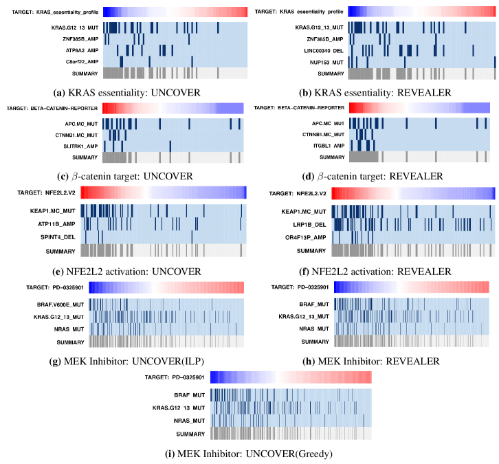
Fig 7: Results of UNCOVER and REVEALER on four cancer datasets from [33].
(a) Solution found by ILP and greedy for KRAS essentiality target. (b) Solution found by ILP and greedy for $\beta$-catenin activation target. (c) Solution found by ILP for MEK inihibitor target. (d) Solution found by greedy for MEK inihibitor target. (e) Solution found by ILP and greedy for NFE2L2 activation target. Each panel shows the value of the target (top row) for various samples (columns), with red being positive and blue being negative values. For each gene in the solution, alterations in each sample are shown in dark blue, while samples not altered are in light blue. The last row shows the alteration profile of the entire solution.

References

- 1. Brennan CW, Verhaak RGW, McKenna A, Campos B, Noushmehr H, Salama SR, et al. The somatic genomic landscape of glioblastoma. Cell. 2013;155(2):462–77. doi:10.1016/j.cell.2013.09.034.
- 2. Cancer Genome Atlas Network. Comprehensive genomic characterization of head and neck squamous cell carcinomas. Nature. 2015;517(7536):576–82. doi:10.1038/nature14129.
- 3. Cancer Genome Atlas Research Network. Comprehensive molecular characterization of clear cell renal cell carcinoma. Nature. 2013;499(7456):43–9. doi:10.1038/nature12222.
- 4. Cancer Genome Atlas Research Network. Integrated genomic characterization of papillary thyroid carcinoma. Cell. 2014;159(3):676–90. doi:10.1016/j.cell.2014.09.050.
- 5. Network CGAR, et al. Integrated genomic characterization of oesophageal carcinoma. Nature. 2017;541(7636):169–175.
- 6. Network CGAR, et al. Integrated Genomic Characterization of Pancreatic Ductal Adenocarcinoma. Cancer cell. 2017;32(2):185.
- 7. Garraway LA, Lander ES. Lessons from the cancer genome. Cell. 2013;153(1):17–37.
- 8. McGranahan N, Swanton C. Clonal heterogeneity and tumor evolution: past, present, and the future. Cell. 2017;168(4):613–628.
- 9. Raphael BJ, Dobson JR, Oesper L, Vandin F. Identifying driver mutations in sequenced cancer genomes: computational approaches to enable precision medicine. Genome Med. 2014;6(1):5.
- 10. Vandin F. Computational Methods for Characterizing Cancer Mutational Heterogeneity. Frontiers in genetics. 2017;8:83.
- 11. Vogelstein B, Papadopoulos N, Velculescu VE, Zhou S, Diaz LA, Kinzler KW. Cancer genome landscapes. science. 2013;339(6127):1546–1558.
- 12. Vaske CJ, Benz SC, Sanborn JZ, Earl D, Szeto C, Zhu J, et al. Inference of patient-specific pathway activities from multi-dimensional cancer genomics data using PARADIGM. Bioinformatics. 2010;26(12):i237–i245.
- 13. Leiserson MDM, Vandin F, Wu HT, Dobson JR, Eldridge JV, Thomas JL, et al. Pan-cancer network analysis identifies combinations of rare somatic mutations across pathways and protein complexes. Nat Genet. 2015;47(2):106–14. doi:10.1038/ng.3168.
- 14. Creixell P, Reimand J, Haider S, Wu G, Shibata T, Vazquez M, et al. Pathway and network analysis of cancer genomes. Nature methods. 2015;12(7):615.
- 15. Kandoth C, McLellan MD, Vandin F, Ye K, Niu B, Lu C, et al. Mutational landscape and significance across 12 major cancer types. Nature. 2013;502(7471):333–339.
- 16. Hanahan D, Weinberg RA. Hallmarks of cancer: the next generation. cell. 2011;144(5):646–674.
- 17. Ciriello G, Cerami E, Sander C, Schultz N. Mutual exclusivity analysis identifies oncogenic network modules. Genome Res. 2012;22(2):398–406. doi:10.1101/gr.125567.111.
- 18. Leiserson MD, Wu HT, Vandin F, Raphael BJ. CoMEt: a statistical approach to identify combinations of mutually exclusive alterations in cancer. Genome biology. 2015;16(1):160.
- 19. Cowley GS, Weir BA, Vazquez F, Tamayo P, Scott JA, Rusin S, et al. Parallel genome-scale loss of function screens in 216 cancer cell lines for the identification of context-specific genetic dependencies. Sci Data. 2014;1:140035.
- 20. Aguirre AJ, Meyers RM, Weir BA, Vazquez F, Zhang CZ, Ben-David U, et al. Genomic Copy Number Dictates a Gene-Independent Cell Response to CRISPR/Cas9 Targeting. Cancer Discov. 2016;6(8):914–929.
- 21. Tsherniak A, Vazquez F, Montgomery PG, Weir BA, Kryukov G, Cowley GS, et al. Defining a Cancer Dependency Map. Cell. 2017;170(3):564–576.
- 22. Mootha VK, Lindgren CM, Eriksson KF, Subramanian A, Sihag S, Lehar J, et al. PGC-1alpha-responsive genes involved in oxidative phosphorylation are coordinately downregulated in human diabetes. Nat Genet. 2003;34(3):267–273.
- 23. Subramanian A, Tamayo P, Mootha VK, Mukherjee S, Ebert BL, Gillette MA, et al. Gene set enrichment analysis: a knowledge-based approach for interpreting genome-wide expression profiles. Proc Natl Acad Sci USA. 2005;102(43):15545–15550.
- 24. Yeang CH, McCormick F, Levine A. Combinatorial patterns of somatic gene mutations in cancer. The FASEB Journal. 2008;22(8):2605–2622.
- 25. Miller CA, Settle SH, Sulman EP, Aldape KD, Milosavljevic A. Discovering functional modules by identifying recurrent and mutually exclusive mutational patterns in tumors. BMC Med Genomics. 2011;4:34. doi:10.1186/1755-8794-4-34.
- 26. Vandin F, Upfal E, Raphael BJ. De novo discovery of mutated driver pathways in cancer. Genome Res. 2012;22(2):375–85. doi:10.1101/gr.120477.111.
- 27. Leiserson MD, Blokh D, Sharan R, Raphael BJ. Simultaneous identification of multiple driver pathways in cancer. PLoS Comput Biol. 2013;9(5):e1003054.
- 28. Kim YA, Madan S, Przytycka TM. WeSME: uncovering mutual exclusivity of cancer drivers and beyond. Bioinformatics. 2016; p. btw242.
- 29. Constantinescu S, Szczurek E, Mohammadi P, Rahnenführer J, Beerenwinkel N. TiMEx: a waiting time model for mutually exclusive cancer alterations. Bioinformatics. 2015; p. btv400.
- 30. Babur Ö, Gönen M, Aksoy BA, Schultz N, Ciriello G, Sander C, et al. Systematic identification of cancer driving signaling pathways based on mutual exclusivity of genomic alterations. Genome biology. 2015;16(1):45.
- 31. Raphael BJ, Vandin F. Simultaneous inference of cancer pathways and tumor progression from cross-sectional mutation data. Journal of Computational Biology. 2015;22(6):510–527.
- 32. Cristea S, Kuipers J, Beerenwinkel N. pathTiMEx: Joint Inference of Mutually Exclusive Cancer Pathways and Their Progression Dynamics. Journal of Computational Biology. 2016;.
- 33. Kim ea Jong. Characterizing genomic alterations in cancer by complementary functional associations. Nature Biotechnology. 2016;34(5):539–546.
- 34. Vandin F, Upfal E, Raphael BJ. De novo discovery of mutated driver pathways in cancer. Genome Res. 2012;22(2):375–385.
- 35. Hochbaum D, Pathria A. Analysis of the Greedy Approach in Problems of Maximum k-Coverage. Naval Research Logistics. 1998;45(6):615–627.
- 36. Mitzenmacher M, Upfal E. Probability and Computing: Randomization and Probabilistic Techniques in Algorithms and Data Analysis. Cambridge university press; 2017.
- 37. Shao DD, Tsherniak A, Gopal S, Weir BA, Tamayo P, Stransky N, et al. ATARiS: computational quantification of gene suppression phenotypes from multisample RNAi screens. Genome Res. 2013;23(4):665–678.
- 38. Solis LM, Behrens C, Dong W, Suraokar M, Ozburn NC, Moran CA, et al. Nrf2 and Keap1 abnormalities in non-small cell lung carcinoma and association with clinicopathologic features. Clin Cancer Res. 2010;16(14):3743–3753.
- 39. Minde DP, Anvarian Z, Rudiger SG, Maurice MM. Messing up disorder: how do missense mutations in the tumor suppressor protein APC lead to cancer? Mol Cancer. 2011;10:101.
- 40. Razick S, Magklaras G, Donaldson IM. iRefIndex: a consolidated protein interaction database with provenance. BMC Bioinformatics. 2008;9:405.
- 41. Kanehisa M, Furumichi M, Tanabe M, Sato Y, Morishima K. KEGG: new perspectives on genomes, pathways, diseases and drugs. Nucleic Acids Res. 2017;45(D1):D353–D361.