Robust principal components for irregularly spaced longitudinal data

Abstract

Consider longitudinal data $x_{ij},$ with $i=1,...,n$ and $j=1,...,p_{i},$ where $x_{ij}$ is the $j-$th observation of the random function $X_{i}\left(.\right)$ observed at time $t_{j}.$ The goal of this paper is to develop a parsimonious representation of the data by a linear combination of a set of $q$ smooth functions $H_{k}\left(.\right)$ ($k=1,..,q)$ in the sense that $x_{ij}\approx\mu_{j}+\sum_{k=1}^{q}\beta_{ki}H_{k}\left(t_{j}\right),$ such that it fulfills three goals: it is resistant to atypical $X_{i}$’s (“case contamination”), it is resistant to isolated gross errors at some $t_{ij}$ (”cell contamination”), and it can be applied when some of the $x_{ij}$ are missing (”irregularly spaced —or ’incomplete’– data”).

Two approaches will be proposed for this problem. One deals with the three goals stated above, and is based on ideas similar to MM-estimation (Yohai 1987). The other is a simple and fast estimator which can be applied to complete data with case- and cellwise contamination, and is based on applying a standard robust principal components estimate and smoothing the principal directions. Experiments with real and simulated data suggest that with complete data the simple estimator outperforms its competitors, while the MM estimator is competitive for incomplete data.

Keywords: Principal components, MM-estimator, longitudinal .data, B-splines, incomplete data.

1 Introduction

Consider longitudinal data $x_{ij},$ with $i=1,...,n$ and $j=1,...,p,$ where $x_{ij}$ is the $j-$th observation of the random function $X_{i}\left(.\right)$ observed at time $t_{j}.$ The goal of this paper is to develop a parsimonious representation of the data by a linear combination of a set of $q$ smooth functions $H_{k}\left(.\right)$ ($k=1,..,q)$ in the sense that

$$x_{ij}\approx\mu_{j}+\sum_{k=1}^{q}\beta_{ik}H_{k}\left(t_{j}\right),$$ (1)

such that it fulfills three goals: it is resistant to atypical $X_{i}$’s (“case contamination”), it is resistant to isolated gross errors at some $t_{j}$ (”cell contamination”), and it can be applied when some of the $x_{ij}$ are missing (”irregularly spaced —or ’incomplete’– data”).

Among the abundant literature on this subject, Bali et al. (2011) propose an approach based on projection pursuit; Boente et al. (2015) and Cevallos (2016) transform the functional data to lower dimensional data through a spline basis representation, to which they apply robust principal components based on the minimization of a robust scale; and Lee et al. (2013) propose a penalized M-estimator. These approaches hold only for complete data with casewise contamination. James et al. (2001) and Yao et al (2005) propose estimators for incomplete data. They require computing sample means and covariances and are therefore not robust.

Two approaches will be proposed for this problem. One deals with the three goals stated above, and is based on ideas similar to MM-estimation (Yohai 1987); the other is a very simple and fast estimator which can be applied to complete data with case- and cellwise contamination. It is based on applying a standard robust principal components estimate and smoothing the principal directions, and will be called the “Naive” estimator.

The contents of the paper are as follows. Sections 2 and 3 present the MM- and the Naive estimators. Sections 4 and 6 compare their performances for complete data to those of former proposals through simulations and a real data example. Sections 8 and 9 compare the performance of MM for incomplete data to that of a former proposal through simulations and a real data example. Finally Sections 10 and 11 give the details of the computation of the MM- and Naive estimates.

2 The “MM” estimator

Let $B_{l}\left(t\right)$ ($l=1,...,m)$ be a basis of B-splines defined on an interval containing $t_{1},...,t_{p}.$ Call $q$ the desired number of components.

For given $\boldsymbol{\alpha}\mathbf{=}[\alpha_{kl}]$, $\boldsymbol{\beta}\mathbf{=[}\beta_{ik}\mathbf{]}$ and $\boldsymbol{\mu}=[\mu_{j}],$ with $i=1,..,n,$ $j=1,...,p,$ $l=1,..,m$ and $k=1,...,q$ define

$$\widehat{x}_{ij}\left(\boldsymbol{\alpha.\beta,\mu}\right)=\mu_{j}+\sum_{k=1}^{q}\beta_{ik}H_{k}\left(t_{j}\right)\$$

with

$$H_{k}\left(t\right)=\sum_{l=1}^{m}\alpha_{kl}B_{l}\left(t\right).$$ (2)

Then the proposed estimator is given by

$$\left(\widehat{\boldsymbol{a}},\widehat{\boldsymbol{\beta}},\widehat{\boldsymbol{\mu}}\right)=\arg\min_{\boldsymbol{\alpha,\beta,\mu}}\sum_{i=1}^{n}\sum_{j\in J_{i}}\widehat{\sigma}_{j}^{2}\rho\left(\frac{x_{ij}-\widehat{x}_{ij}\left(\boldsymbol{\alpha,\beta,\mu}\right)}{\widehat{\sigma}_{j}}\right).$$ (3)

where $\widehat{\sigma}_{j}$ are previously computed local scales and $J_{i}=\{j:x_{ij}$ is non-missing$\}.$ If $\rho\left(t\right)=t^{2}$ and the data are complete, the estimator coincides with the classical principal components (PC) estimator. The matrix of principal directions (“eigenvectors”) is

$$\mathbf{E=B}\widehat{\mathbf{\alpha}}^{\prime}\in R^{p\times q},$$ (4)

where $\mathbf{B}$ is the matrix with elements $b_{jl}=B_{l}\left(t_{j}\right).$

This estimator will henceforth be called “MM-estimator”. It is computed iteratively, starting from a deterministic initial estimator. Since the whole procedure is complex, the details are postponed to Section 10.

A robust measure of “unexplained variance” for $q$ components is defined as

$$V_{q}=\sum_{i=1}^{n}\sum_{j\in J_{i}}\widehat{\sigma}_{j}^{2}\rho\left(\frac{x_{ij}-\widehat{x}_{ij}\left(\widehat{\boldsymbol{\alpha}}\boldsymbol{,}\widehat{\boldsymbol{\beta}}\boldsymbol{,}\widehat{\boldsymbol{\mu}}\right)}{\widehat{\sigma}_{j}}\right),$$

and the “proportion of explained variance” is given by

$$u_{q}=1-\frac{V_{q}}{V_{0}},$$ (5)

where $V_{0}$ is obtained from (3) with $\mathbf{\alpha=0}$ and $\mathbf{\beta=0.}$

The number of spline knots is of the form $[p/K],$ where $[.]$ denotes the integer part. Choosing $K$ through cross-validation did not yield better results than using a fixed value. After a series of exploratory simulations it was decided that $K=6$ yielded satisfactory results.

3 The “naive” estimator

A simple proposal complete data is introduced. It consists of four steps:

1. “Clean” local outliers by applying a robust smoother to each $\mathbf{x}_{i}$ and then imputing atypical values.

2. Compute $q$ ordinary robust PC’s of the “cleaned” $\mathbf{x}_{i}$s.

3. Smooth the $q$ eigenvectors using a B-spline basis.

4. Orthogonalize them.

A robust “proportion of unexplained variance” can be computed as explained in Section 11.

In order to simplify the exposition, the details are given in Section 11.

4 Complete data: simulation

Instead of using arbitrary functions for the simulation scenarios, it was considered more realistic to take them from a real data set. We chose the Low Resolution Spectroscopy (LRS) data set (Bay 1999), which contains $n=531$ spectra, on the“red” and “blue” ranges. We deal with the “blue” data, which has $p=44.$

The first two classical components account respectively for 60% and 33% of the variability. It was therefore considered that $q=2$ components was a good choice.

The first four classical eigenvectors $\mathbf{e}_{k}$ ($k=1,..,4)$ and the mean vector $\boldsymbol{\mu}$ were computed, and a polynomial approximation was fitted to them, so that they can be obtained for any $p.$ The first two $\mathbf{e}_{k}$s and the mean vector are plotted in Figure 1

Figure 1: LRS Blue data: first two eigenvectors and mean vector.

For given $p$ and $q$ the data are generated as multivariate normal with mean $\boldsymbol{\mu}$ and covariance matrix

$$\boldsymbol{\Sigma}\mathbf{=}\left[\sigma_{ij}\right]=\sum_{k=1}^{q}\pi_{k}\mathbf{e}_{k}\mathbf{e}_{k}^{\prime}+\pi_{0}\mathbf{I,}$$ (6)

where now $\mathbf{\mu}$ and $\mathbf{e}_{k}$ are the original vectors “scaled” to the interval $[1,p]$ rather than the original $[1,43],$ and $\mathbf{I}$ is the $p$-dimensional identity matrix. The last term induces noise. The simulations were run for $q=2$ and 3 and under different configurations of the $\pi^{\prime}$s.

4.1 Contamination

Two types of contamination are considered. In case-wise contamination, a proportion $\varepsilon_{\mathrm{case}}$ of cases are replaced by $\mathbf{x}_{0}=K\sqrt{\lambda_{1}}\mathbf{c,}$where $\mathbf{c}$ is orthogonal to $\mathbf{e}_{k},$ $k=1,..,q,$ and $\lambda_{1}$ is the first eigenvalue of $\mathbf{\Sigma.}$ The factor $\sqrt{\lambda_{1}}$ simplifies the choice of the range of $K.$ Two choices for $\mathbf{c}$ were employed: one was simply $\mathbf{e}_{q+1},$ the $(q+1)$-th eigenvector of $\mathbf{\Sigma,}$ and the other was a random direction orthogonal to $\mathbf{e}_{k},$ $k=1,..,q.$ Since the qualitative results yielded by both options were similar, only those corresponding to the first one are shown.

The outlier size $K$ ranges between 0.10 and 3, in order to find the “most malign” configurations for each estimator.

Figure 2 shows for $p=50$ and $q=2$ three “typical” cases and a case outlier with $K=1.2$.

Figure 2: Simulation: three “typical” cases and one case outlier (–)

In cell-wise contamination, each cell is contaminated at random with probability $\varepsilon_{\mathrm{cell}}=1/p.$ This means that each case has in average one outlier, but about 63% of the cases have some outliers. In contaminated cells, $x_{ij}$ is replaced by $x_{ij}+K\sigma_{jj}.$ Here $K$ ranges between 1 and 7.

4.2 Evaluation

Two issues have to be considered to evaluate an estimator’s performance at a given simulation scenario. The first is the precision with which the PCs reconstruct the data, which means measuring the differences between the fitted and the observed values. It was observed that even for “good” data, the distribution of the prediction errors $x_{ij}-\widehat{x}_{ij}$ may have heavy tails. For this reason the fit of each estimator was evaluated through its prediction Mean Absolute Error (MAE), which was considered as less sensitive than the Mean Squared Error to some atypical values.

For a given estimator call $\widehat{x}_{ij}$ the fitted values. For case-wise contamination call $I$ the set of non-contaminated rows. Then define for a data set $[x_{ij}]$

$$\mathrm{MAE=ave}\left\{|x_{ij}-\widehat{x}_{ij}|:i\in I,\ j=1,..,p\right\}.$$

For cell-wise contamination the average is taken over all cells:

$$\mathrm{MAE=ave}\left\{|x_{ij}-\widehat{x}_{ij}|:i=1,..,n,\ j=1,..,p\right\},$$

the justification being that the estimator should be able to “guess” the true value at the contaminated cell because of the assumed underlying smoothness of the data.

Finally, for each estimator the average MAE over all Monte Carlo replications is computed.

The second issue is the estimation of the “true” PCs. To this end, the angle $\alpha$ between the estimated subspace and the subspace generated by $\{\mathbf{e}_{k},k=1,..,q\}$ was computed. Since it was thought that $\sin\left(\alpha\right)$ would be easier to interpret (because it ranges between 0 and one), the averages of $\sin\left(\alpha\right)$ are reported.

5 Simulation results

The estimators involved in the simulation are: Classic, “Naive”, MM, the S-estimator of Boente and Salibian-Barrera (2015) using a B-spline basis, and the LTS estimator of Cevallos (2016). The R code for the S and LTS estimators was kindly supplied by the authors. Unfortunately it was not possible to obtain the code for the estimator of Lee et al. (2013).

The dimension was set at $p=50.$ The number of components was chosen as $q=$ 2 and 3. Different configurations for the $\pi_{j}$s in (6) were employed. The results given here are for $q=2$ and $\pi_{1}=0.6,$ $\pi_{2}=0.3,$ $\pi_{3}=0.05.$ Since the qualitative results yielded by $q=3$ and by other configurations of the $\pi_{j}$s are similar, they are not reported here. The number of replications is 200. It would probably be more realistic to fix a predetermined proportion of “explained variance” (say, 90%) and let each estimator choose $q$ accordingly. While this can be done with the Classic, Naive and MM estimators, it cannot be done with the S and LTS estimators.

“Efficiency” will be loosely defined as “similitude with the Classical estimator when $\varepsilon_{\mathrm{case}}=\varepsilon_{\mathrm{cell}}=0$”.

Table 1 shows the maximum averages (over $K$) of the MAEs for $p=50$ and two components.

$n$	$\varepsilon_{\mathrm{case}}$	$\varepsilon_{\mathrm{cell}}$	Class.	Naive	MM	S	LTS
100	0	0	557	563	595	563	600
	0.1	0	2663	565	675	564	638
	0.2	0	2633	604	1051	591	2708
	0	0.02	2701	585	617	1567	1593
200	0	0	282	287	298	285	411
	0.1	0	1334	288	351	287	414
	0.2	0	1323	334	547	287	1406
	0	0.02	892	288	295	664	764

Table 1: Simulation: maximum MAEs of estimators

Table 2 shows the maximum mean $\sin\left(\alpha\right)$ for the same scenarios.

$n$	$\varepsilon_{\mathrm{case}}$	$\varepsilon_{\mathrm{cell}}$	Class.	Naive	MM	S	LTS
50	0	0	0.014	0.015	0.025	0.018	0.055
	0.1	0	0.998	0.016	0.079	0.020	0.070
	0.2	0	0.999	0.036	0.194	0.042	0.878
	0	0.02	0.619	0.016	0.039	0.021	0.058
200	0	0	0.011	0.012	0.017	0.016	0.210
	0.1	0	0.998	0.013	0.085	0.019	0.211
	0.2	0	0.999	0.059	0.190	0.020	0.879
	0	0.02	0.287	0.012	0.020	0.019	0.211

Table 2: Simulation: maximum sin($\alpha$) of estimators

5.1 Discussion

Comparing the maximum MAEs it can be concluded that

• The Naive, S and MM estimators appear as reasonably efficient

• For case-wise contamination, the Naive and S estimators appear as the best, the latter being slightly better; LTS and MM have similar acceptable performances for $\varepsilon_{\mathrm{case}}=0.1;$ when $\varepsilon_{\mathrm{case}}=0.2,$ MM and especially LTS have poorer performances

• For cell-wise contamination, the Naive and MM estimators are practically unaffected by outliers, while the other estimators are clearly affected by them.

The results of Table 2 for $\varepsilon_{\mathrm{cell}}=0$ parallel those of Table 1. However, comparing the results for $\varepsilon_{\mathrm{cell}}=0.02$ with those for $\varepsilon_{\mathrm{cell}}=\varepsilon_{\mathrm{case}}=0$ it is seen that S and LTS are almost unaffected by cell outliers!. The seeming contradiction between these results and those of Table 1 is explained by the fact that in (1), even if the $H_{k}$s are correctly estimated, the $\beta$s must be robustly estimated too, and it is here that these two estimators fail.

Examination of intermediate results reveals that the “weak spot” of MM lies at the starting values, which require the estimation of a covariance matrix, which has to be deterministic, fast, resistant to cell-wise outliers and computable for incomplete data. The price for so many requirements is a decrease in robustness for large $\varepsilon_{\mathrm{case}}.$ See Section 10 for details.

6 Complete data: a real example

The chosen data set is the “red” range of the LRS data (Bay 1999), which has $n=531$ spectra with $p=49.$

The estimated proportions of explained variance with two components are

Classic	Naive	MM
0.91	0.85	0.88

It was therefore considered reasonable to choose $q=2$ components.

Since our goal is assessing how well do the fitted values approximate the data (rather than outlier detection), estimates will be evaluated by their MAEs. For a given estimate let the MAE of row $i=1,..,n$ be

$$m_{i}=\mathrm{ave}\left\{\left|x_{ij}-\widehat{x}_{ij}\right|:j=1,...,p\right\},\$$ (7)

The overall MAEs (averages of the $m_{i})$ are

184160162160384.fragments 184160162160384\begin{tabular}[c]{ccccc}\hline\cr Class.&Naive&MM&S&LTS\\ \hline\cr\lx@intercol\hfil 184\lx@intercol &\lx@intercol\hfil 160\lx@intercol &\lx@intercol\hfil 162\lx@intercol &\lx@intercol\hfil 160\lx@intercol &\lx@intercol\hfil 384\lx@intercol\\ \hline\cr\end{tabular}\ \ \ .

Class.NaiveMMSLTSClass.NaiveMMSLTS

Figure 3 shows the quantiles (in log scale) of the MAEs corresponding to the different estimates.

Figure 3: LRS data: quantiles of estimates’ MAEs: Classical (—), Naive(- -), MM (…), S (-.-.) and LTS (– –)

The MM, Naive and S estimate give similar results; the classical estimate gives slightly poorer results, and LTS shows a poor fit. The quantiles of the classical estimate are larger than those of MM, Naive and S, except for the top 4%. This fact can be attributed to outlying cases. Figure 4 shows three “typical” cases corresponding to the quartiles of the Naive estimate’s $m_{i}$ (dashed lines) and to the 0.96-quantile (solid line). The latter appears as totally atypical. One may thus interpret that the classical estimate attempts to fit all cases, including the atypical ones, at the expense of the typical ones, while the robust estimates downweight the latter.

Figure 4: LRS data: three “typical” cases (dashed line) and an outlier (full line).

For a closer look at the behavior of LTS, Figure 5 shows the fit to case 338, a typical one. It is seen that the Naive, S and MM estimators give good fits and the Classical performs a bit worse, while LTS gives wrong values at the extremes. This behavior occurs in most cases of this data set.

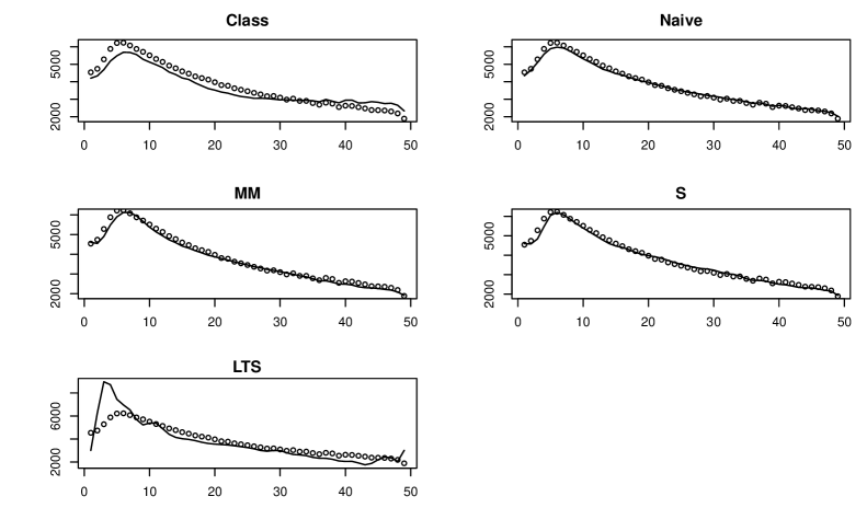
Figure 5: LRS data: case 338 (o) and fits by different estimates (—)

7 Computing times

The next table shows the average computing times in seconds for $n=4p$ and number of components $q,$ on a PC with a 3.60 GH processor with 4 cores. Here “S” denotes the parallelized version of the S estimator’s code.

$p$	$n$	$q$	Naive	MM	LTS	S
50	200	2	0.07	2.65	11.80	22.91
		4	0.07	3.66	12.69	23.13
100	400	2	0.25	14.75	19.18	103.80
		4	0.25	22.24	21.98	107.37
200	800	2	1.20	105.73	32.10	710.31
		4	1.21	157.84	38.60	742.25

Table 3: Computing times of estimators

It is seen that the Naive estimator is by far the fastest, and S is the slowest; MM is faster than LTS for $p\leq 100,$ but slower otherwise. The computing times of S and LTS are unaffected by $q;$ the computing time of MM increases with $q$ (because components are computed one at a time)

As a final conclusion: considering efficiency, robustness and speed, it may be concluded that for complete data, the Naive estimator is to be recommended.

8 Incomplete data: a real example

We begin our treatment of incomplete data by introducing a new data set, which belongs to the Multicenter AIDS Cohort Study (MACS) and is available at https://statepi.jhsph.edu/macs/pdt.html. It contains $n=305$ cases, with $p=48.$ The number of observations per case varies between 1 and 9. There is a total of 2001 measurements, which yields a “decimation rate”

$$d=\frac{\#(\mathrm{measurements})}{np}=0.137.$$ (8)

The MM-estimator was compared to the procedure “Principal Analysis by Conditional Estimation” (PACE) (Yao et al 2005), which is implemented in the package fdapace available at the authors’ web site.

The proportions of explained variance for one and two components were 0.92 and 0.98 for PACE, and 0.77 and 0.81 for MM. It was decided to take $q=2.$

The overall MAEs of PACE and MM are respectively 93.2 and 87.5. Figure 6 compares the quantiles of the MAEs $m_{i}$ (7) from both estimates. It is seen that their performances are similar, with MM doing slightly better.

Figure 6: MACS data: case MAEs of PACE(—) and MM ( -)

The proportions of explained variance from MM are much lower than those from PACE. The reason is that they employ different measures of variability. Outliers in the first principal axes inflate the ordinary variance but contribute little to a robust variance. A similar phenomenon is observed in (Maronna et al, 2006, ps. 213-14).

9 Incomplete data: simulation:

Two scenarios were chosen for the simulations. One is the same employed in Section 4. The other is based on the MACS data set; the mean vector $\mathbf{\mu}$ and the first principal directions $\mathbf{e}_{k}$ of the data were estimated with PACE, and then employed in the same way as with the LRS data. They will be called “LRS scenario” and “MACS scenario”.

For each scenario a complete data set was generated, and then each cell was kept at random with probability $d,$ the “decimation rate” as in (8), and the others set as “missing”. The values of $d$ were 0.25 and 0.5. The outlier size $K$ ranged between 1 and 6. The values of $\pi_{1},$ $\pi_{2}$ and $\pi_{3}$ are the same as in Section 4. The dimension was set as $p=50,$ and the sample size $n$ took on the values 100 and 200. Since both values yielded similar results, only those corresponding to the first one are shown.

Table 4 shows the results for the MACS scenario with $q=2$. It is seen that MM is practically unaffected by the contamination. The MAEs of PACE are heavily affected by both case- and cell-contamination; the angle is also heavily affected by case contamination, but not so much by cell contamination.

$d$	$\varepsilon_{\mathrm{case}}$	$\varepsilon_{\mathrm{cell}}$	MAE		Angle
			PACE	MM	PACE	MM
0.5	0	0	26.49	23.64	0.066	0.058
	0.05	0	155.71	24.61	0.996	0.072
	0.1	0	210.43	26.46	0.999	0.096
	0	0.02	55.40	23.72	0.087	0.058
	0	0.05	97.74	23.80	0.112	0.058
0.25	0	0	28.97	25.27	0.097	0.097
	0.05	0	156.31	25.62	0.987	0.100
	0.1	0	209.98	27.02	0.996	0.112
	0	0.02	64.13	25.70	0.132	0.097
	0	0.05	111.27	27.46	0.173	0.098

Table 4: Simulation with MACS scenario: maximum MAEs and mean angles for $p=50$ and $n=100$

Figure 7 shows the MAEs and mean angles as a function of $K$ for $d=0.5.$ $\varepsilon_{\mathrm{case}}=0.1$ and $\varepsilon_{\mathrm{cell}}=0,$ and Figure 8 does the same for $\varepsilon_{\mathrm{case}}=0$ and $\varepsilon_{\mathrm{cell}}=0.05.$ The values for $K=0$ are those corresponding $\varepsilon_{\mathrm{case}}=\varepsilon_{\mathrm{cell}}=0.$ It is seen that in all cases MM remains practically constant with $K;$ when $\varepsilon_{\mathrm{case}}=0.1$ PACE is clearly affected when $K\geq 2;$ and when $\varepsilon_{\mathrm{cell}}=0.05$ its MAEs are also affected but the angle shows more resistance.

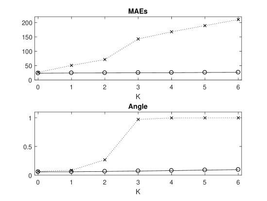
Figure 7: Simulation with MACS scenario: MAEs of PACE(x) and MM (o) as a function of outlier size $K$ for $\varepsilon_{\mathrm{case}}=0.1$ and $d=0.5$

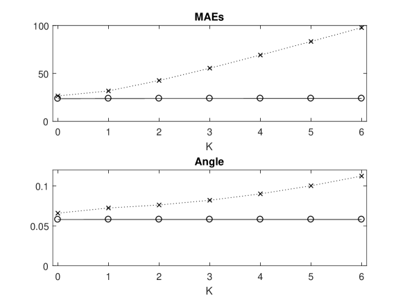
Figure 8: Simulation with MACS scenario: MAEs of PACE(x) and MM (o) as a function of outlier size $K$ for $\varepsilon_{\mathrm{cell}}=0.05$ and $d=0.5$

A surprising feature of Table 4 is that for $\varepsilon_{\mathrm{case}}=\varepsilon_{\mathrm{cell}}=0$ MM is slightly better than PACE. Changing the random generator seed yielded similar results.

Table 5 shows the results for the LRS scenario.

$d$	$\varepsilon_{\mathrm{case}}$	$\varepsilon_{\mathrm{cell}}$	MAE		Angle
			PACE	MM	PACE	MM
0.5	0	0	778	637	0.171	0.082
	0.05	0	2664	819	0.644	0.086
	0.1	0	3978	697	0.968	0.109
	0	0.02	1400	637	0.174	0.082
	0	0.05	2296	655	0.186	0.087
0.25	0	0	778	1000	0.182	0.267
	0.05	0	2562	1057	0.667	0.275
	0.1	0	3651	1078	0.937	0.283
	0	0.02	1532	1066	0.193	0.276
	0	0.05	2556	1182	0.230	0.278

Table 5: Simulation with LRS scenario: maximum MAEs and mean angles for $p=50$ and $n=100$

It is seen that when $d=0.5$ MM is unaffected by contamination and again outperforms PACE in all cases. When $d=0.25$ MM has a lower MAE for $\varepsilon_{\mathrm{case}}>0$. When $\varepsilon_{\mathrm{case}}=0.$ PACE has lower MAE and mean Angle than MM when $\varepsilon_{\mathrm{cell}}=0,$ and a lower maximum mean Angle when $\varepsilon_{\mathrm{cell}}>0.$ Since PACE makes a clever use of the information when data is sparse, this result is more on line with what would be expected.

It can be concluded that MM is resistant to both case- and cell-contamination, that its efficiency with respect to PACE is high for decimation rate $d=0.5,$ while it may depend on the data structure for $d=0.25.$

10 Computing algorithm of the MM-estimator

The computation proceeds one component at a time. Define for $i=1,..,n$ and $j=1,...,p$

$$J_{i}=\{j:\ x_{ij}~{}\text{is non-missing}\},\ \text{\ }I_{j}=\{i:\ x_{ij}~{}\text{is non-missing}\}.$$

At the beginning (“zero components”): apply robust nonparametric regression to obtain robust and smooth local location and scale values $\widehat{\mu}_{0j}$ and $\widehat{\sigma}_{0j},$ $j=1,...,p$ as follows. Let $S\left(.,.\right)$ be a robust smoother. Let $m_{j}$ be a location M-estimator of $\{x_{ij},~{}i\in I_{j}\};$ then the set $\{\widehat{\mu}_{0j},~{}j=1,..,p\}$ is obtained by applying $S$ to $\left(\tau_{j},m_{j},j=1,...,p\right).$ Let $s_{j}$ be a $\tau$-scale of $\{x_{ij}-\widehat{\mu}_{0j},i\in I_{j}\}$; then the set $\{\widehat{\sigma}_{0j},j=1,,,,p\}$ is obtained by applying $S$ to $\left(\tau_{j},s_{j},j=1,..,p\right).$ The chosen smoother was the robust version of Loess (Cleveland 1979) with a span of 0.3.

Let $y_{ij}^{\left(0\right)}=x_{ij}-\widehat{\mu}_{0j}.$ Compute the “unexplained variance”

$$V_{0}=\frac{1}{N}\sum_{i=1}^{n}\sum_{j\in I_{j}}\widehat{\sigma}_{0}{}_{j}^{2}\rho\left(\frac{y_{ij}^{\left(0\right)}}{\widehat{\sigma}_{0}{}_{j}}\right)~{}~{}\mathrm{with~{}}\ N=\sum_{j=1}^{p}\mathrm{card}\left(I_{j}\right).$$

For component 1 use the $y_{ij}^{\left(0\right)}$ as input and compute

$$\left(\widehat{\boldsymbol{a}}^{\left(1\right)},\widehat{\boldsymbol{\beta}}^{\left(1\right)},\boldsymbol{\mu}^{\left(1\right)}\right)=\arg\min_{\mathbf{\alpha,\beta,}\boldsymbol{\mu}}\sum_{i=1}^{n}\sum_{j\in I_{j}}\widehat{\sigma}_{0j}^{2}\rho\left(\frac{y_{ij}^{\left(0\right)}-\widehat{y}_{ij}^{\left(0\right)}\left(\boldsymbol{\alpha,\beta,\mu}\right)}{\widehat{\sigma}_{0j}}\right).$$ (9)

The minimum is computed iteratively, starting from a deterministic initial estimator to be described in Section 10.2.

Compute the residuals $y_{ij}^{\left(1\right)}=y_{ij}^{\left(0\right)}-\widehat{y}_{ij}^{\left(0\right)}\left(\widehat{\boldsymbol{\alpha}}\boldsymbol{,}\widehat{\boldsymbol{\beta}}\boldsymbol{,}\widehat{\boldsymbol{\mu}}\right).$ Apply a smoother to compute local residual scales $\widehat{\sigma}_{1}{}_{j}$ and the “unexplained variance” with one component:

$$V_{1}=\frac{1}{N}\sum_{i=1}^{n}\sum_{j\in I_{j}}\widehat{\sigma}_{1}{}_{j}^{2}\rho\left(\frac{y_{ij}^{\left(1\right)}}{\widehat{\sigma}_{1}{}_{j}}\right).$$

For component $k$ we have

$$\left(\widehat{\boldsymbol{a}}^{\left(k\right)},\widehat{\boldsymbol{\beta}}^{\left(k\right)},\boldsymbol{\mu}^{\left(k\right)}\right)=\arg\min_{\mathbf{\alpha,\beta,}\boldsymbol{\mu}}\sum_{i=1}^{n}\sum_{j\in I_{j}}\widehat{\sigma}_{k-1,j}^{2}\rho\left(\frac{y_{ij}^{\left(k-1\right)}-\widehat{y}_{ij}^{\left(k-1\right)}\left(\boldsymbol{\alpha,\beta,\mu}\right)}{\widehat{\sigma}_{k-1,j}}\right).$$ (10)

Each component is orthogonalized with respect to the former ones. The procedure stops either at a fixed number of components or when the proportion of explained variance (5) is larger than a given value (e.g. 0.90).

10.1 The iterative algorithm

Computing each component requires an iterative algorithm and starting values. The algorithm is essentially one of “alternating regressions”.

Recall that at each step $\boldsymbol{\alpha\in}R^{m}$ and $\boldsymbol{\beta\in}R^{n}$ are one-dimensional. Put as usual $\psi=\rho^{\prime}$ and $W(s)=\psi\left(s\right)/s.$ Put for brevity $h\left(t\right)=\sum_{l=1}^{m}\alpha_{l}B_{l}\left(t\right)$ where $B_{i}$ are the elements of the spline basis.

Differentiating the criterion in (10) yields a set of estimating equations that can be written in fixed-point form, yielding a “weighted alternating regressions” scheme. To simplify the notation the superscript $\left(k-1\right)$ will be dropped from $y_{ij}^{\left(k-1\right)}$ and $\widehat{y}_{ij}^{\left(k-1\right)}.$ Put

$$w_{ij}=w_{ij}\left(\boldsymbol{\alpha,\beta,\mu}\right)=W\left(\frac{y_{ij}-\widehat{y}_{ij}\left(\boldsymbol{\alpha,\beta,\mu}\right)}{\widehat{\sigma}_{k-1,j}}\right).$$

Then $\mu_{j}$ and $\beta_{i}$ can be expressed as weighted residual means and weighted univariate least squares regressions, respectively:

$$\mu_{j}=\frac{1}{\sum_{i\in I_{j}}w_{ij}}\sum_{i\in I_{j}}w_{ij}\left(y_{ij}-\beta_{i}h\left(t_{j}\right)\right),$$

$$\beta_{i}=\frac{\sum_{j\in J_{i}}w_{ij}h\left(t_{j}\right)\mathbf{(}y_{ij}-\mu_{j})}{\sum_{j\in J_{i}}w_{ij}h\left(t_{j}\right)^{2}}$$

and $\boldsymbol{\alpha}$ is the solution of

$$\sum_{i=1}^{n}\sum_{j\in J_{i}}w_{ij}\left(y_{ij}-\mu_{j}\right)\beta_{i}\mathbf{b}\left(t_{j}\right)=\sum_{i=1}^{n}\sum_{j\in J_{i}}w_{ij}\beta_{i}^{2}\mathbf{b}\left(t_{j}\right)\mathbf{b}\left(t_{j}\right)^{\prime}\boldsymbol{\alpha}$$

with $\mathbf{b}\left(t\right)=\left(B_{1}\left(t\right),...,B_{l}\left(t\right)\right)$’.

At each iteration the $w_{ij}$ are updated. It can be shown that the criterion descends at each iteration.

10.2 The initial values

For each component, initial values for $\boldsymbol{\alpha}$ and $\boldsymbol{\beta}$ are needed. They should be deterministic, since subsampling would make the procedure impractically slow.

10.2.1 The initial $\boldsymbol{\alpha}$

For $k,l\in\left\{1,...,p\right\}$ call $N_{kl}$ the number of cases that have values in both $t_{k}$ and $t_{l}:$

$$N_{kl}=\#\left(I_{k}\cap I_{l}\right).$$

In longitudinal studies, many $N_{kl}$ may null or very small.

Compute a (possibly incomplete) $p\times p$ matrix $\boldsymbol{\Sigma=[}\sigma_{kl}\boldsymbol{]}$ of pairwise robust covariances of $\left(y_{ik},y_{il}:i\in I_{k}\cap I_{l}\right)$ with the Gnanadesikan-Kettenring procedure:

$$\mathrm{Cov}\left(X,Y\right)=\frac{1}{4}\left(S\left(X+Y\right)^{2}-S\left(X-Y\right)^{2}\right),$$

where $S$ is a robust dispersion. Preliminary simulations led to the choice of the $Q_{n}$ estimator of Rousseeuw and Croux (1993).

More precisely; for $N_{kl}\geq 3$ compute $\sigma_{kl}$ as above. If $\min_{kl}N_{kl}$ is “large enough” (here: $\geq 10)$ use the resulting $\mathbf{\Sigma.}$

Otherwise apply a two-dimensional smoother to improve $\mathbf{\Sigma}$ and to fill in the missing values. The bivariate Loess was employed for this purpose.

Then compute the first eigenvector $\mathbf{e}$ of $\boldsymbol{\Sigma}$ (note that $\boldsymbol{\Sigma}$ is not guaranteed to be positive definite and hence further principal components may be unreliable). Given $\mathbf{e,}$ smooth it using the spline basis. This $\mathbf{\alpha}$ follows from (4).

10.2.2 The initial $\boldsymbol{\beta}$

For $i=1,...,n$ the initial $\beta_{i}$ is a robust univariate regression of $y_{ij}$ on $h\left(t_{j}\right)$ $(j\in J_{i}),$ namely the $L_{1}$ regression, which is fast and reliable.

Note that only cellwise outliers matter at this step.

10.3 The final adjustment

Note that the former steps yield only an approximate solution of (3) since the components are computed one at a time. In order to improve the approximation a natural procedure is as follows. After computing $q$ components we have a $p\times q$-matrix $\mathbf{U}$ of principal directions with elements

$$u_{jk}=\sum_{l=1}^{m}B_{l}\left(t_{j}\right)\alpha_{kl},$$

an $n\times p$-matrix of weights $\mathbf{W.}$ and a location vector $\mathbf{\mu.}$ Then a natural improvement is –keeping $\mathbf{U}$ and $\mathbf{\mu}$ fixed– to recompute the $\beta$s by means of univariate weighted regressions with weights $w_{ij}.$ Let $\mathbf{\beta}_{i.}=[\beta_{ik},k=1,..,p],$ and set

$$\mathbf{\beta}_{i}=\arg\min_{\mathbf{\beta\in}R^{q}}\sum_{j\in J_{i}}w_{ij}\left(x_{ij}-\mu_{j}-\mathbf{U\beta}\right)^{2}.$$

The effect of this step in the case of complete data is negligible, but it does improve the estimator’s behavior for incomplete data.

However, it was found out that the improvement is not good enough when the data are very sparse. For this reason another approach was used, namely, to compute $\mathbf{\beta}_{i}$ as a regression M-estimate. Let $\mathbf{z}_{i}=(x_{ij}-\mu_{j}:j\in J_{i})$ and $\mathbf{V=[}v_{jk}\mathbf{]}$ with $v_{jk}=u_{jk}$ for $j\in J_{i}.$ Then $\mathbf{\beta}_{i}$ is a bisquare regression estimate of $\mathbf{z}_{i}$ on $\mathbf{V,}$ with tuning constant equal to 4, using $L_{1}$ as a starting estimate. Note that here only cell outliers matter, and therefore $L_{1}$ yields reliable starting values. The estimator resulting from this step does not necessarily coincide with (3), but simulations show that it is much better than the “natural” adjustment described above when the data are very sparse.

11 The “naive” estimator: details

In step 1 of Section 3, compute for each $\mathbf{x}_{i}$ robust local location and scatter estimates $\widetilde{\mu}_{i},\widetilde{\sigma}_{i}$. The “cleaned” values are

$$\widetilde{x}_{ij}=\widetilde{\mu}_{i}+\widetilde{\sigma}_{i}\psi\left(\frac{x_{ij}-\widetilde{\mu}_{i}}{\widetilde{\sigma}_{i}}\right),$$

where $\psi$ is the bisquare $\psi$-function with tuning constant equal to 4.

The ordinary robust PCs of step 2 are computed using the cleaned data $\widetilde{x}_{ij}$ with the S-M estimator of (Maronna 2005). Call $\{\widehat{\mathbf{x}}_{i}^{\left(q\right)}\}$ the fit for $q$ components and put $r_{i}^{\left(q\right)}=$ $\left\|\mathbf{x}_{i}-\widehat{\mathbf{x}}_{i}^{\left(q\right)}\right\|,$ $i=1,...,n.$ Then the estimator minimizes $S\left(r_{i}^{\left(q\right)},\ \ i=1,..,n\right)$ where $S$ is the bisquare M-scale. The “proportion of unexplained variance” is

$$\frac{S\left(r_{i}^{\left(q\right)},\ \ i=1,..,n\right)}{S\left(r_{i}^{\left(0\right)},\ \ i=1,..,n\right)}.$$

The number of knots in step 3 is chosen through generalized cross-validation.

12 References

Bali, J.L., Boente, G., Tyler, D.E. and Wang, J-L. (2011). Robust functional principal components: a projection-pursuit approach. The Annals of Statistics, 39, 2852–2882.

Bay, S. D. (1999), The UCI KDD Archive [http://kdd.ics.uci.edu], University of California, Irvine, Dept. of Information and Computer Science.

Boente, G. and Salibian-Barrera, M. (2015). S-Estimators for Functional Principal Component Analysis. Journal of the American Statistical Association, 110, 1100-1111.

Cevallos Valdiviezo, H. (2016). On Methods for Prediction Based on Complex Data with Missing Values and Robust Principal Component Analysis, PhD thesis, Ghent University (supervisors Van Aelst S. and Van den Poel, D.).

Cleveland, W.S. (1979). Robust Locally Weighted Regression and Smoothing Scatterplots. Journal of the American Statistical Association, 74, 829-836.

James, G., Hastie, T.G., and Sugar, C.A. (2001). Principal Component Models for Sparse Functional Data. Biometrika, 87, 587-602.

Lee, S., Shin, H. and Billor, N. (2013). M-type smoothing spline estimators for principal functions. Computational Statistics and Data Analysis, 66, 89-100.

Maronna, R. (2005). Principal components and orthogonal regression based on robust scales. Technometrics, 47¸ 264-273.

Maronna, R.A., Martin, R.D. and Yohai, V.J. (2006). Robust Statistics: Theory and Methods. John Wiley and Sons, Chichester.

Rousseeuw, P.J. and Croux, C. (1993). Alternatives to the Median Absolute Deviation. Journal of the American Statistical Association, 88, 1273–1283.

Yao, F., Müller, H-G. and Wang, J-L. (2005). Functional Data Analysis for Sparse Longitudinal Data. Journal of the American Statistical Association, 100, 577-590.

Yohai, V.J. (1987). High Breakdown-Point and High Efficiency Robust Estimates for Regression. The Annals of Statistics, 15, 642-656.