BAGAN: Data Augmentation with Balancing GAN

Abstract

Image classification datasets are often imbalanced, characteristic that negatively affects the accuracy of deep-learning classifiers. In this work we propose balancing GAN (BAGAN) as an augmentation tool to restore balance in imbalanced datasets. This is challenging because the few minority-class images may not be enough to train a GAN. We overcome this issue by including during the adversarial training all available images of majority and minority classes. The generative model learns useful features from majority classes and uses these to generate images for minority classes. We apply class conditioning in the latent space to drive the generation process towards a target class. The generator in the GAN is initialized with the encoder module of an autoencoder that enables us to learn an accurate class-conditioning in the latent space. We compare the proposed methodology with state-of-the-art GANs and demonstrate that BAGAN generates images of superior quality when trained with an imbalanced dataset.

1 Introduction

The accuracy of image classification techniques can significantly deteriorate when the training dataset is imbalanced, i.e. when available data is not uniformly distributed between the different classes. Imbalanced datasets are common and a traditional approach to mitigate this problem is to augment the dataset by introducing additional minority-class images derived by applying simple geometric transformations to original images, e.g. rotations or mirroring. This augmentation approach may disrupt orientation-related features when these are relevant. In this work we propose a balancing generative adversarial network (BAGAN) as an augmentation tool to restore the dataset balance by generating new minority-class images. Since these images are scarce in the initial dataset, it is challenging to train a GAN for generating new ones. To overcome this issue, the proposed methodology includes in the adversarial training all data from minority and majority classes at once. This enables BAGAN to learn underlying features of the specific classification problem starting from all images and then to apply these features for the generation of new minority-class images. For example, let us consider the classification of road traffic signs [1]. All warning signs share the same external triangular shape. Once BAGAN learns to draw this shape from one of the signs, we can apply it for drawing any other one. Since BAGAN learns features starting from all classes whereas the goal is to generate images for the minority classes, a mechanism to drive the generation process toward a desired class is needed. To this end, in this work we apply class conditioning on the latent space [2, 3]. We initialize the discriminator and generator in the GAN with an autoencoder. Then, we leverage this autoencoder to learn class conditioning in the latent space, i.e. to learn how the input of the generative model should look like for different classes. Additionally, this initialization enables us to start the adversarial training from a more stable point and helps mitigating convergence problems arising with traditional GANs [4, 5, 6, 7]. The main contributions of this work are:

• An overall approach to train GANs with an imbalanced dataset while specifically aiming to generate minority-class images.

• An autoencoder-based initialization strategy that enables us to a) start training the GAN from a good initial solution, and b) learn how to encode different classes in the latent space of the generator.

• An empirical evaluation of the proposed BAGAN methodology against the state of the art.

Experimental results empirically demonstrate that the proposed BAGAN methodology outperforms state-of-the-art GAN approaches in terms of variety and quality of the generated images when the training dataset is imbalanced. In turn, this leads to a higher accuracy of final classifiers trained on the augmented dataset.

2 Background

In recent years generative adversarial neural networks (GANs) [8, 9, 7] have been proposed as a tool to artificially generate realistic images. The underlying idea is to train a generative network in adversarial mode against a discriminator network.

A well known problem of generative adversarial models is that while they learn to fool the discriminator they may end up drawing one or few foolish examples. This problem is known as mode collapse [8, 4, 5, 6]. In this work, our aim is to augment an imbalanced image classification dataset to restore its balance. It is of paramount importance that the augmented dataset is variable enough and does not include a continuously repeating example, thus we need to avoid mode collapse. To this end, different approaches have been proposed. Possible solutions are: explicitly promoting image diversity in the generator loss [10, 4], letting the generator predict future changes of the discriminator and adapt against these [11], let the discriminator distinguish the different classes [2, 12], applying specific regularization techniques [5, 6], and coupling GANs with autoencoders [4, 13, 14, 15].

In this work we apply the latter approach and couple GAN and autoencoding techniques. The cited approaches include additional modules in the GAN to embed an autoencoder all along the training. In the proposed BAGAN methodology we apply a more pragmatic approach and use an autoencoder to initialize the GAN modules close to a good solution and far from mode collapse. Since our goal is to generate images specifically for the minority classes, we train a generator that is controllable in terms of the image class it draws, similarly to the state-of-the-art ACGAN methodology [2]. Nonetheless, ACGAN is not specifically meant for imbalanced datasets and turns to be flawed when targeting the generation of minority-class images.

3 Motivating Example

State-of-the-art GANs are not suitable to deal with imbalanced datasets [16] and, to the best of our knowledge, the proposed BAGAN methodology is the first one to specifically address this topic. Before going through details of the proposed approach, let us demonstrate with a simple example why it is difficult to apply existing GAN techniques to tackle the problem at hand. Let us consider the classification of handwritten digits, starting from an imbalanced version of the MNIST dataset [17] where we remove ${97.5\%}$ of the available zeros from the training set.

A trivial idea would be to use a traditional GAN [8, 9, 18], train it by using all the available data, generate many random samples, find the ${0}$ instances and use these for augmenting the dataset. This approach cannot be applied in general: if the generator ${G}$ in the GAN is trained to fool the discriminator ${D}$ by generating realistic images, it will better focus on the generation of majority classes to optimize its loss function while collapsing away the modes related to the minority class. On the other hand, training a GAN by using only the minority-class images is not really an option because minority-class images are scarce. In this example, after removing ${97.5\%}$ of the zeros, we are left with about 150 minority-class images. In general, it is difficult to train a GAN starting from a very little dataset, the GAN must have many examples to learn from [19].

(a) ACGAN discriminator.

(b) BAGAN discriminator.

Figure 1: Discriminator architectures for ACGAN and BAGAN.

(a) ACGAN.

(b) Proposed BAGAN.

Figure 2: Ten zero-digit images generated with ACGAN and the proposed BAGAN when trained with an imbalanced version of MNIST where ${97.5\%}$ of the zeros were dropped.

(a) Autoencoder training.

(b) GAN initialization.

(c) GAN training.

Figure 3: The three training steps of the proposed BAGAN methodology.

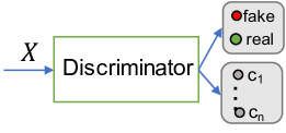
A different approach is to train the GAN with majority and minority classes jointly and to let the GAN distinguish between different classes explicitly. During training, the generator is explicitly asked to draw images of every class and to let the discriminator believe that the generated images are real images of the desired classes. While doing so, the generator is explicitly rewarded for drawing realistic images of each class including the minority classes. To the best of our knowledge, the only method implementing this approach presented in literature so far is ACGAN [2] where the generator input can be conditioned to draw a target class. In ACGAN, the discriminator has two outputs, one to discriminate between real and fake images ${X}$, and the other to classify ${X}$ in terms of its class ${c}$, Figure 1(a). During training, the generator is explicitly asked to draw images ${{{X}_{{c}}}}$ for each class ${c}$. Generator parameters are adjusted to maximize the superposition of two components. The first component is the log-likelihood of generating an image ${{{X}_{{c}}}}$ considered real by the discriminator. The second component is the log-likelihood of generating an image ${{{X}_{{c}}}}$ that the discriminator associates with the class ${c}$. We observed that, when a dataset is imbalanced, these two components become contradictory for the minority class. This can be explained as follows. Let us assume that at a point in time the generator converged into a solution where it generates minority-class images with real-word quality. These images would be indistinguishable by the discriminator from the ones in the training dataset. Since in the training dataset minority-class images are scarce, when a minority-class image is passed to the discriminator during training it is most likely a fake image. To optimize its loss function the discriminator has to associate the fake label to all minority-class images. At this point, the two generator objectives are contradictory and the generator can either draw an image that looks real or one that is representative of the minority class but cannot achieve these two goals at once. In turn, the generator can be rewarded for drawing images that look real and are not representative of the target minority class. This fact deteriorates the quality of generated images. Images for the imbalanced MNIST example generated by ACGAN for the ${0}$ digit are shown in Figure 2(a). In this work we propose BAGAN that applies class conditioning as ACGAN but differs on the following points.

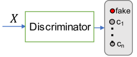
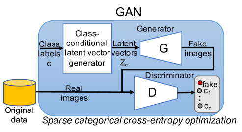
First, the BAGAN discriminator has a single output that returns either a problem-specific class label ${c}$ or the label fake, Figure 1(b). The discriminator ${D}$ is trained for associating to the images generated by ${G}$ the label fake, and to real images ${{X}_{{c}}}$ their class label ${c}$. The generator is trained to avoid the fake label and match the desired class labels. Since this is now defined as a single objective rather than as a superposition of two objectives, by construction it cannot contradict itself and the generator is never rewarded for the generation of images ${{{X}_{{c}}}}$ that look real if the discriminator does not match them with the desired class label ${c}$.

Second, BAGAN couples GAN and autoencoding techniques to provide a precise selection of the class conditioning and to better avoid mode collapse. Images for the imbalanced MNIST example generated by BAGAN are of superior quality, Figure 2(b).

4 BAGAN

The proposed BAGAN methodology aims to generate realistic minority-class images for an imbalanced dataset. It exploits all available information of the specific classification problem by including in the BAGAN training majority and minority classes jointly. GAN and autoencoding techniques are coupled to leverage the strengths of the two approaches. GANs generate high-quality images whereas autoencoders converge towards good solution easily [7]. Several authors suggest to couple GANs and autoencoders [4, 13]. Nonetheless these works are not directly meant to drive the GAN generative process towards specific classes. It is not easy to generalize them to enable the GAN to distinguish between different classes. As explained in the motivating example, in this work we apply class conditioning as suggested by Odena et al. [2] to embed class knowledge in BAGAN.

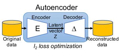
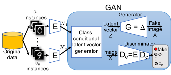
We apply a pragmatic use of autoencoders to initialize the GAN close to a good solution and far from mode collapse. Additionally, we apply the encoder part of the autoencoder to infer the distribution of the different classes in the latent space. The autoencoder-based GAN initialization is achievable by using the same network topology in the autoencoder and GAN modules, Figures 3(a) and 3(b). The decoding stage ${\Delta}$ of the autoencoder matches the topology of the generator ${G}$. The encoding stage ${E}$ of the autoencoder matches the topology of the first layers of the discriminator ${{D}_{e}}$. In BAGAN, the knowledge in the autoencoder is transferred into the GAN modules by initializing the parameter weights accordingly, Figure 3(b). To complete the discriminator, a final dense layer ${{D}_{d}}$ with a softmax activation function translates the latent features into the probability that the image is fake or that it belongs to one of the problem classes ${c}_{1}$ — ${c}_{n}$. When the GAN modules are initialized, a class-conditional latent vector generator is set up by learning the probability distribution of the images in the latent space for the different classes. Then, all the weights in the generator and discriminator are fine tuned by carrying out a traditional adversarial training, Figure 3(c). Overall, the BAGAN training approach is organized in the three steps show in Figure 3: a) autoencoder training, b) GAN initialization, and c) adversarial training.

Autoencoder training. The autoencoder is trained by using all the images in the training dataset. The autoencoder has no explicit class knowledge, it processes all images from majority and minority classes unconditionally. In this work we apply $l_{2}$ loss minimization for the autoencoder training.

GAN initialization. Differently from the autoencoder, the generator ${G}$ and the discriminator ${D}$ have explicit class knowledge. During the adversarial training, ${G}$ is asked to generate images for different classes, and ${D}$ is asked to label the images either as fake or with a problem-specific class label ${c}$. At the moment the GAN is initialized, the autoencoder knowledge is transferred into the GAN modules by initializing ${G}$ with the weights in the decoder ${\Delta}$, and the first layers of the discriminator ${{D}_{e}}$ with the weights of the encoder ${E}$, Figure 3(b). The last layer of the discriminator ${{D}_{d}}$ is a dense layer with a softmax activation function and generates the final discriminator output. The weights of this last layer are initialized at random and learnt during the adversarial training.

The discriminator initialization is used simply to include in ${D}$ meaningful features that can help in classifying images. The initialization of the generator has a deeper reason. When adversarial training starts, the generator ${G}$ is equivalent to the decoder ${\Delta}$. Thus a latent vector ${Z}$ input to the generator ${G}$ is equivalent to a point in the latent space of the autoencoder, i.e. ${Z}$ can be seen as the output of ${E}$ or the input of ${\Delta}$. Thus, the encoder ${E}$ maps real images into the latent space in use by ${G}$. We leverage this fact to learn a good class conditioning before to start the adversarial training, i.e. we define how a latent vector ${{Z}_{{c}}}$ should look like for an image of class ${c}$.

We model a class in the latent space with a multivariate normal distribution $\mathcal{N}_{{c}}=\mathcal{N}(\mu_{{c}},\Sigma_{{c}})$ with mean vector $\mu_{{c}}$ and covariance matrix $\Sigma_{{c}}$. For each class ${c}$, we compute $\mu_{{c}}$ and $\Sigma_{{c}}$ to match the distribution of ${{Z}_{{c}}}={E}({{X}_{{c}}})$ considering all real images ${{X}_{{c}}}$ of class ${c}$ available in the training dataset. We initialize with these probability distributions the class-conditional latent vector generator, that is a random process that takes as input a class label ${c}$ and returns as output a latent vector ${{Z}_{{c}}}$ drawn at random from $\mathcal{N}_{{c}}$. During the adversarial training, the probability distributions $\mathcal{N}_{{c}}$ are considered invariant forcing the generator not to diverge from the initial class encoding in the latent space.

Table 1: Target datasets’ information including resolution, number of classes, and per-class image distribution statistics for the training set.

			Training images per class
Dataset name	Resolution	Classes	Min	Median	Mean	Max
MNIST	28$\times$28	10	5421	5936	6000	6742
CIFAR-10	32$\times$32	10	5000	5000	5000	5000
Flowers	224$\times$224	5	533	599	634	798
GTSRB	64$\times$64	43	210	600	911	2250

(a) Real image samples

(b) BAGAN

(c) ACGAN

(d) Simple GAN

Figure 4: Five representative samples for each class (row) in the CIFAR-10 dataset. For each class, these samples are obtained with generative models trained after dropping from the training set $40\%$ of the images of that specific class.

Adversarial training. During the adversarial training, data flows in batches through the generator ${G}$ and the discriminator ${D}$ and their weights are fine tuned to optimize their loss functions. The discriminator classifies an input image as belonging to one of the $n$ problem-specific classes or as being fake. For each batch we supply, $1/(n+1)$ of the total images are fake, i.e. we provide the best possible balance for the fake class. The fake data is generated as output of ${G}$ that takes as inputs latent vectors ${{Z}_{{c}}}$ extracted from the class-conditional latent vector generator. In turn, the class-conditional latent vector generator takes as input uniformly distributed class labels ${c}$, i.e. the fake images are uniformly distributed between the problem-specific classes. When training the discriminator ${D}$ we optimize the sparse categorical cross-entropy loss function to match the class labels for real images and the fake label for the generated ones.

For every batch learnt by the discriminator, a batch of the same size is learnt by the generator ${G}$. To this end, a batch of conditional latent vectors ${{Z}_{{c}}}$ is drawn at random by applying a uniform distribution on the labels ${c}$. These vectors are processed by the generator and the output images are fed into the discriminator. The parameters in ${G}$ are optimized to match the labels selected by the discriminator with the labels ${c}$ used to generate the images.

5 Results

We validate the proposed methodology on a set of four datasets. We consider: MNIST [17], CIFAR-10 [20], Flowers [21], and GTSRB [1]. The former two datasets are well known, Flowers is a small dataset including real photos of five categories of flowers that we reshaped to the resolution of 224x224, and GTSRB is a traffic sign recognition dataset. Details on these datasets are shown in Table 1. The first three datasets are balanced, GTSRB is imbalanced. We force imbalance in the first three datasets by selecting a class and dropping a significant amount of its instances from the training set. We repeat this process for each class and train different generative models for each resulting imbalanced dataset. The following results for each class are always obtained when training with that class as minority class and we refer to the images left out from the training set as dropped images. Since GTSRB is already imbalanced, we do not further imbalance it.

(a) Real image samples

(b) BAGAN

(c) ACGAN

(d) Simple GAN

Figure 5: Five representative samples generated for the three most represented majority classes in the GTSRB dataset.

(a) Real image samples

(b) BAGAN

(c) ACGAN

(d) Simple GAN

Figure 6: Five representative samples generated for the three least represented minority classes in the GTSRB dataset.

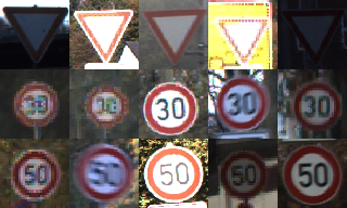
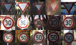
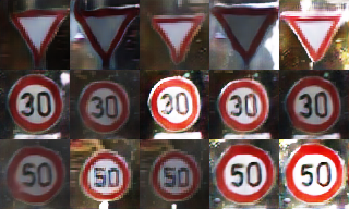
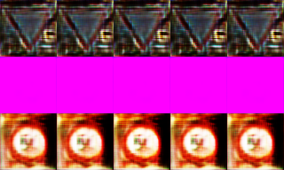
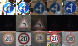
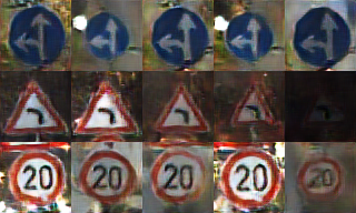
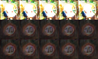
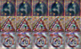
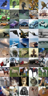
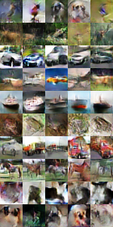
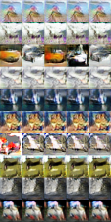
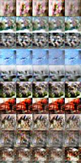
We compare the proposed BAGAN model with the state-of-the-art ACGAN model [2]. To the best of our knowledge, ACGAN is the only methodology presented in literature so far to consider class conditioning to draw images of a target class starting from a dataset including multiple classes (Section 3). Both BAGAN and ACGAN are trained on the target datasets by using majority and minority classes jointly. We also consider a simple GAN approach that learns to draw the minority-class images by training only on that class. For a fair comparison, we limit the architecture changes between the considered methodologies (BAGAN, ACGAN, and GAN). The difference between BAGAN and ACGAN are those described in this paper (i.e. discriminator output topology and autoencoder-based initialization). For the simple GAN, we adjust the reference ACGAN discriminator output to discriminate only between real and fake images, and we remove the class conditioning for the generator input (this GAN is trained only over images from the minority class). Figures 4, 5, and 6 show a qualitative analysis of representative images generated for CIFAR-10 and for the three most and least represented classes in GTSRB. For CIFAR-10 we show results only for minority-class images. For each class, 40% of that class images are dropped, generative models are trained, and randomly generated images are shown, Figure 4. For CIFAR-10, the simple GAN collapses towards the generation of a single image example per class. To train this GAN we use only 3000 minority-class images (40% of the minority-class images are dropped and majority classes are not included in the training). Adversarial networks need many examples to learn drawing new images [19] and in this case the simple GAN collapses. For ACGAN and BAGAN this issue is less relevant because they can learn features from minority and majority classes jointly. To better understand the different behavior of ACGAN and BAGAN, let us focus on the GTSRB dataset Figures 5 and 6. This dataset is originally imbalanced and we train the generative models without modifying it. For the majority classes, both ACGAN and BAGAN return high-quality results, Figures 5(c) and 5(b). Nonetheless, ACGAN fails in drawing images for the minority classes and collapses towards the generation of a single example for each class, Figure 6(c). In some cases ACGAN produces images that are not representative of the desired class, e.g. the second row in Figure 6(c) should be a warning sign whereas a speed limit is drawn. BAGAN is never rewarded for drawing a realistic image if this does not represent the desired class. Thus, BAGAN does not exhibit this behavior.

Figure 7: Accuracy of the images generated by the considered methodologies when varying the percentage of minority-class images dropped before training the generative models. The accuracy is based on a ResNet-18 classifier trained without dropping any image.

5.1 Quantitative Assessment of Generated Images

Since our goal is to leverage the generative model to augment an imbalanced dataset by generating additional minority-class images, we aim at the following goals:

1. Generated images must represent the desired class.

2. Generated images must not be repetitive.

3. Generated images must be different from the real ones already available in the training set.

Missing to meet a) means that the generative model is not capable to generate images that accurately represent the target class and they look either as real examples of other classes or they do not look real. Missing to meet b) means that the generative model collapsed to the generation of a single or few modes. Missing to meet c) means that we simply learnt to redraw the available training images. We assess the quality of the generated images on the basis of these three goals.

Figure 8: Structural similarity for generated image couples (SSIM couples, $y$ axis) when varying the percentage of images dropped from the training set ($x$ axis).

Figure 9: Average accuracy for the minority-class achieved with a ResNet-18 classifier trained with the augmented dataset whose balance is restored after dropping a percentage of minority-class images.

Accuracy of the generated images. To verify that the images generated by the considered methodologies are representative of the desired classes, we classify them by means of a deep learning model trained on the whole original dataset and we verify if the predicted classes match the target ones. In this work we use a ResNet-18 model [22]. Results are shown in Figure 7. The simple GAN returns the worst accuracy for generated images. The proposed BAGAN approach is generally better than the other approaches and generates images that the ResNet-18 model can classify with the highest accuracy. We observe again that a strong imbalance can significantly deteriorate the quality of generated images with an accuracy that decreases as the percentage of dropped images increases. This phenomenon is most evident for ACGAN when targeting the MNIST dataset.

Variability of generated images. We measure similarity between two images by means of the structural image similarity SSIM [23]. This metric predicts human perceptual similarity judgment, it returns one when the two images are identical and decreases as differences become more relevant. To verify that generated images are diverse, for each class we repeatedly generate a couple of images and measure their similarity SSIM. Figure 8 shows this diversity analysis for the considered datasets averaged over all classes. For MNIST, CIFAR-10, and Flowers, we vary the percentage of minority-class images dropped within the set $\{40,60,80,90,95,97.5\}$, whereas for GTSRB we use the originally imbalanced dataset. We include in the analysis also a reference value that is the average SSIM between real image couples of the same class. When taking a random couple of real images for CIFAR-10 or Flowers, these have so little in common that the reference SSIM gets very close to zero. In general real images are always more variable than the generated ones (lower SSIM). Variability in images generated by the simple GAN approach is very little and sampled image couples have SSIM very close to one. The proposed BAGAN methodology exhibit the best variability with respect to GAN and ACGANwith SSIM values closest to the reference. For CIFAR-10 and Flowers, all methodologies deteriorate for strong imbalances with SSIM values that increase with the percentage of images dropped from the training set.

Image diversity with respect to the training set. To assess the variability of generated images with respect to the ones already available in the training set. We compute the SSIM between generated images and their closest real neighbour. We compare this value with respect to the image variability in the training set, i.e. the SSIM value between a real image and its closest real neighbour. These SSIM values are very close to each others meaning that there was no overfitting. This statement holds for all the considered methodologies. In particular SSIM values of about 0.8, 0.25, 0.05, and 0.5 are measured respectively for MNIST, CIFAR-10, Flowers, and GTSRB.

5.2 Quality of the Final Classification

We finally assess the accuracy of a deep-learning classifier trained on an augmented dataset. For MNIST, CIFAR-10, and Flowers, for each class we: 1) select this class as minority class, 2) generate an imbalanced dataset by dropping a percentage of images for this class from the training set, 3) train the considered generative models, 4) augment the imbalanced dataset to restore its balance by means of the generative models, 5) train a ResNet-18 classifier for the augmented dataset, and 6) measure the classifier accuracy for the minority class over the test set. Since GTSRB is already imbalanced, for this dataset we skip steps 1) and 2). Augmentations obtained by the generative models are compared to the plain imbalanced dataset and to an horizontal mirroring augmentation approach (mirror) where new minority-class images are generated by mirroring the ones available in the training set.

Accuracy results averaged over the different classes are shown in Figure 9. The proposed BAGAN methodology returns the best accuracy for GTSRB and most of the time also for MNIST. These two datasets are characterized by features sensible to the image orientation and the mirroring approach as expected returns the worst accuracy results because it disrupts these features. For CIFAR-10 and Flowers the best accuracy is achieved by using the mirroring approach. Mirroring for these datasets does not disrupt any feature, qualitatively the mirrored images are as good as the original ones. The BAGAN approach still provides the best accuracy when compared to ACGAN and GAN.

From this analysis we conclude that BAGAN is superior to other state-of-the-art adversarial generative networks when aiming at the generation of minority-class images starting from an imbalanced dataset. Additionally we conclude that: when it is not easy to augment a dataset with traditional techniques because of orientation-related features, BAGAN can be applied to improve the final classification accuracy.

6 Conclusion

In this work we presented a methodology to restore the balance of an imbalanced dataset by using generative adversarial networks. In the proposed BAGAN framework the generator and the discriminator modules are initialized by means of an autoencoder to start the adversarial training from a good solution and to learn how different classes should be represented in the latent space.

We compared the proposed methodology against the state of the art. Empirical results demonstrate that BAGAN is superior to other generative adversarial networks when aiming at the generation of high quality images starting with an imbalanced training set. This in turn results in a higher accuracy of deep-learning classifiers trained over the augmented dataset where the balance has been restored.

References

- [1] J. Stallkamp, M. Schlipsing, J. Salmen, and C. Igel. Man vs. computer: Benchmarking machine learning algorithms for traffic sign recognition. Neural Networks, (0):–, 2012.
- [2] Augustus Odena, Christopher Olah, and Jonathon Shlens. Conditional image synthesis with auxiliary classifier GANs. In Doina Precup and Yee Whye Teh, editors, Proceedings of the 34th International Conference on Machine Learning, volume 70 of Proceedings of Machine Learning Research, pages 2642–2651, International Convention Centre, Sydney, Australia, 06–11 Aug 2017. PMLR.
- [3] Anh Nguyen, Alexey Dosovitskiy, Jason Yosinski, Thomas Brox, and Jeff Clune. Synthesizing the preferred inputs for neurons in neural networks via deep generator networks. In D. D. Lee, M. Sugiyama, U. V. Luxburg, I. Guyon, and R. Garnett, editors, Advances in Neural Information Processing Systems 29, pages 3387–3395. Curran Associates, Inc., 2016.
- [4] A. Srivastava, L. Valkov, C. Russell, M. U. Gutmann, and C. Sutton. VEEGAN: Reducing Mode Collapse in GANs using Implicit Variational Learning. ArXiv e-prints, May 2017.
- [5] Kevin Roth, Aurelien Lucchi, Sebastian Nowozin, and Thomas Hofmann. Stabilizing training of generative adversarial networks through regularization. In I. Guyon, U. V. Luxburg, S. Bengio, H. Wallach, R. Fergus, S. Vishwanathan, and R. Garnett, editors, Advances in Neural Information Processing Systems 30, pages 2015–2025. Curran Associates, Inc., 2017.
- [6] Naveen Kodali, Jacob D. Abernethy, James Hays, and Zsolt Kira. How to train your DRAGAN. CoRR, abs/1705.07215, 2017.
- [7] M. Lucic, K. Kurach, M. Michalski, S. Gelly, and O. Bousquet. Are GANs Created Equal? A Large-Scale Study. ArXiv e-prints, #nov# 2017.
- [8] I. J. Goodfellow, J. Pouget-Abadie, M. Mirza, B. Xu, D. Warde-Farley, S. Ozair, A. Courville, and Y. Bengio. Generative Adversarial Networks. ArXiv e-prints, June 2014.
- [9] Alec Radford, Luke Metz, and Soumith Chintala. Unsupervised representation learning with deep convolutional generative adversarial networks. CoRR, abs/1511.06434, 2015.
- [10] Min Lin. Softmax GAN. CoRR, abs/1704.06191, 2017.
- [11] Luke Metz, Ben Poole, David Pfau, and Jascha Sohl-Dickstein. Unrolled generative adversarial networks. CoRR, abs/1611.02163, 2016.
- [12] T. Salimans, I. Goodfellow, W. Zaremba, V. Cheung, A. Radford, and X. Chen. Improved techniques for training gans. ArXiv e-prints, June 2016.
- [13] A. Nguyen, J. Clune, Y. Bengio, A. Dosovitskiy, and J. Yosinski. Plug & play generative networks: Conditional iterative generation of images in latent space. ArXiv e-prints, November 2016.
- [14] V. Dumoulin, I. Belghazi, B. Poole, O. Mastropietro, A. Lamb, M. Arjovsky, and A. Courville. Adversarially Learned Inference. ArXiv e-prints, June 2016.
- [15] J. Donahue, P. Krähenbühl, and T. Darrell. Adversarial Feature Learning. ArXiv e-prints, May 2016.
- [16] Luis Perez and Jason Wang. The effectiveness of data augmentation in image classification using deep learning. CoRR, abs/1712.04621, 2017.
- [17] Y. Lecun, L. Bottou, Y. Bengio, and P. Haffner. Gradient-based learning applied to document recognition. Proceedings of the IEEE, 86(11):2278–2324, Nov 1998.
- [18] Tero Karras, Timo Aila, Samuli Laine, and Jaakko Lehtinen. Progressive growing of GANs for improved quality, stability, and variation. In International Conference on Learning Representations, 2018.
- [19] Swaminathan Gurumurthy, Ravi Kiran Sarvadevabhatla, and Venkatesh Babu Radhakrishnan. Deligan : Generative adversarial networks for diverse and limited data. CoRR, abs/1706.02071, 2017.
- [20] Alex Krizhevsky. Learning multiple layers of features from tiny images. Master’s thesis, 2009.
- [21] Image classification using flowers dataset, 2018. https://cloud.google.com/ml-engine/docs/flowers-tutorial.
- [22] K. He, X. Zhang, S. Ren, and J. Sun. Deep residual learning for image recognition. In 2016 IEEE Conference on Computer Vision and Pattern Recognition (CVPR), pages 770–778, June 2016.
- [23] Zhou Wang, A. C. Bovik, H. R. Sheikh, and E. P. Simoncelli. Image quality assessment: from error visibility to structural similarity. IEEE Transactions on Image Processing, 13(4):600–612, April 2004.
- [24] A. Dosovitskiy and T. Brox. Generating Images with Perceptual Similarity Metrics based on Deep Networks. ArXiv e-prints, February 2016.