Can we use linear response theory to assess geoengineering strategies?

Abstract

Geoengineering can control only some climatic variables but not others, resulting in side-effects. We investigate in an intermediate-complexity climate model the applicability of linear response theory (LRT) to the assessment of a geoengineering method. This application of LRT is twofold. First, our objective (O1) is to assess only the best possible geoengineering scenario by looking for a suitable modulation of solar forcing that can cancel out or otherwise modulate a climate change signal that would result from a rise in carbon dioxide concentration [CO₂] alone. Here we consider only the cancellation of the expected global mean surface air temperature $\Delta\langle[T_{s}]\rangle$. It is in fact a straightforward inverse problem for this solar forcing, and, considering an infinite time period, we use LRT to provide the solution in the frequency domain in closed form as $f_{s}(\omega)=(\Delta\langle[T_{s}]\rangle(\omega)-\chi_{g}(\omega)f_{g}(\omega))/\chi_{s}(\omega)$, where the $\chi$’s are linear susceptibilities. We provide procedures suitable for numerical implementation that apply to finite time periods too. Second, to be able to utilize LRT to quantify side-effects, the response with respect to uncontrolled observables, such as regional averages $\langle T_{s}\rangle$, must be approximately linear. Therefore, our objective (O2) here is to assess the linearity of the response. We find that under geoengineering in the sense of (O1), i.e., under combined greenhouse and required solar forcing, the asymptotic response $\Delta\langle[T_{s}]\rangle$ is actually not zero. This turns out not to be due to nonlinearity of the response under geoengineering, but rather a consequence of inaccurate determination of the linear susceptibilities $\chi$. The error is in fact due to a significant quadratic nonlinearity of the response under system identification achieved by a forced experiment. This nonlinear contribution can be easily removed, which results in much better estimates of the linear susceptibility, and, in turn, in a fivefold reduction in $\Delta\langle[T_{s}]\rangle$ under geoengineering practice. This correction dramatically improves also the agreement of the spatial patterns of the predicted linear and the true model responses. However, considering (O2), such an agreement is not perfect and is worse in the case of the precipitation patterns as opposed to surface temperature. Some evidence suggests that it could be due to a greater degree of nonlinearity in the case of precipitation.

Geoengineering strategies with the aim of mitigating climate change are receiving increasing attention,Allen et al. (2014); National Research Council (2015a, b); Lenton and Vaughan (2013); Ferraro, Highwood, and Charlton-Perez (2014); Kravitz et al. (2011); Kravitz (2018); Helwegen et al. (2019); Stilgoe (2019); Collomb (2019) not only because of their potential to solve one of the greatest challenges faced by modern society, but also because of the great risk that such an unprecedented endeavor entails. Here we would like to advocate that the study of climate change in general, and geoengineering in particular, would benefit from response theory Kubo (1966); Ruelle (2009) and the theory of nonautonomous dynamical systems. Sell (1967a, b); Romeiras, Grebogi, and Ott (1990); Crauel and Flandoli (1994); Crauel, Debussche, and Flandoli (1997); Arnold (1998); Kloeden and Rasmussen (2011); Carvalho, Langa, and Robinson (2013) These mathematical tools were introduced into climate science many years ago,Leith (1975); Bell (1980); Nicolis, Boon, and Nicolis (1985) but only recently have they started to really gain traction. Cionni, Visconti, and Sassi (2004); Gritsun and Branstator (2007); Kirk-Davidoff (2009); Majda, Gershgorin, and Yuan (2010); Cooper, Esler, and Haynes (2013); Lucarini and Sarno (2011); Good, Gregory, and Lowe (2011); Ragone, Lucarini, and Lunkeit (2016); Lucarini, Ragone, and Lunkeit (2017); Herein et al. (2015, 2017); Bódai and Tél (2012); Drótos, Bódai, and Tél (2015, 2016) The first application of response theory to the study and efficient assessment of geoengineering in particular was by Kravitz and MacMartin. MacMartin and Kravitz (2016) They assessed the linearity of the response, but regarding global averages only. However, regional temperature responses to radiative forcing can be nonlinear,Cao et al. (2015); Winton (2013); Good et al. (2015); Lucarini, Ragone, and Lunkeit (2017) and there has been an indication Cao et al. (2015) that they can be nonlinear in the case of geoengineering too. We show that it is possible to describe in a concise and general way the response of the climate system to two or more forcings with given time-dependent modulations. In particular—and this is the case of interest in geoengineering—if a forcing is given, one can arrange the time modulation of $N$ other forcings in such a way as to achieve a desired time-dependent change for $N$ climatic observables of interest. The pitfall of this approach is that (a) the response of any other observable is, in principle, uncontrolled and (b) nonlinearities can become more and more relevant as forcings are added to the system. This indicates that there are some fundamental caveats in the setup of geoengineering strategies.

I Introduction: Using response theory to formulate geoengineering strategies and outcomes

First we summarize briefly the existing mathematical tools (Sec. I.1) that will provide us with the framework to describe the geoengineering problem as an inverse problem (O1) (Sec. I.2). We will then elucidate the utility of this inverse problem approach and compare it with the alternative control problem and other approaches (Sec. I.3), and we will subsequently provide the context for the need to assess geoengineering strategies (O2) (Sec. I.4).

I.1 Elements of response theory

In nonautonomous dissipative dynamical systems, like the climate system, given in the form

$$\dot{x}=F(x)+\epsilon g(x,t),$$ (1)

the response of the system to an external forcing $g(x,t)$ can be unambiguously defined in terms of the so-called snapshot attractor Romeiras, Grebogi, and Ott (1990) of the system, and the natural probability distribution or the measure $\mu(x,t)$ supported by it. This applies also to chaotic systems, when the snapshot attractor is a fractal object. Both the attractor and the measure are unique objects; they are defined by an ensemble of trajectories initialized in the infinite past. The time dependence of the snapshot attractor, also called a pullback attractor, Crauel and Flandoli (1994); Arnold (1998); Chekroun, Simonnet, and Ghil (2011) and its measure give what is often termed the “forced response,” and their geometrical details at any instant describe (statistical aspects of) the internal variability in a conceptually sound sense. Drótos, Bódai, and Tél (2015)

For a scalar observable $\Psi(x)$ too, the (forced) response is uniquely given by a projection of the measure. Response theory Risken (1996); Abramov and Majda (2008); Ruelle (2009) asserts that the most basic ensemble-based statistics, the mean $\langle\Psi\rangle(t)=\int\mathrm{d}x\,\Psi(x)\mu(x)(t)$ can be decomposed into linear ($j=1$) and nonlinear ($j>1$) contributions:

$$\Delta\langle\Psi\rangle(t)=\langle\Psi\rangle(t)-\langle\Psi\rangle_{0}=\sum_{j=1}^{\infty}\epsilon^{j}\langle\Psi\rangle^{(j)}(t),$$ (2)

where the first-order, i.e., linear, term can be obtained as

$$\langle\Psi\rangle^{(1)}(t)=\int\mathrm{d}x\,\Psi(x)\int^{\infty}_{-\infty}\mathrm{d}\tau\,(\exp[(t-\tau)L_{F}(x)][L_{g}(x,\tau)\bar{\mu}(x)])(x,t,\tau),$$ (3)

where $\bar{\mu}(x)$ is the natural invariant measure of the autonomous system ($g=0$), and the operators are defined as $L_{F}\mu=-\mathrm{div}(F\mu)$ and $L_{g}\bar{\mu}=-\mathrm{div}(g\bar{\mu})$. In (2), $\langle\Psi\rangle_{0}$ is the unperturbed ($\epsilon=0$) expectation, and the series converges only if the forcing $\epsilon g(x,t)$ is small enough. If the forcing depends on time in a multiplicative fashion, $g(x,t)=g(x)f(t)$, then we can write

$$\langle\Psi\rangle^{(1)}(t)=G_{\Psi}^{(1)}(t)\ast f(t)=\int^{\infty}_{-\infty}\mathrm{d}\tau\,G_{\Psi}^{(1)}(\tau)f(t-\tau),$$ (4)

where the Green’s function is implied by Eqs. (3) and (4) to be

$$G_{\Psi}^{(1)}(t)=\int\mathrm{d}x\,\Psi(x)(\exp[tL_{F}(x)][L_{g}(x)\bar{\mu}(x)])(x,t).$$ (5)

Note that the higher-order terms $\langle\Psi\rangle^{(j)}$ can be expressed as multiple convolution integrals involving multitime Green’s functions.Lucarini, Ragone, and Lunkeit (2017) Taking the Fourier transform (FT) of Eq. (4), we have, via the convolution theorem,Katznelson (1976) a response formula in the frequency domain:

$$\langle\Psi\rangle^{(1)}(\omega)=\chi_{\Psi}^{(1)}(\omega)f(\omega),$$ (6)

where $\chi_{\Psi}^{(1)}(\omega)=\mathrm{FT}[G_{\Psi}^{(1)}(t)]$ is called the linear susceptibility.

I.2 The geoengineering problem

It has been proposed National Research Council (2015b) that the effect of greenhouse forcing can be mitigated by applying another external forcing to the Earth system by some geoengineering means that has, in a way, an opposing effect. There are various types of forcing that can achieve this, but here we will consider those—generically referred to as “solar-radiation management” (SRM) Ricke, Morgan, and Allen (2010); Ricke et al. (2012)—that can be modeled by a modulation of the solar constant. We will call this simply the “solar forcing.” Clearly, these are means that modulate the shortwave incoming radiation. Readily proposed geoengineering methods include a fleet of reflective satellites of large Sun-facing surface area put into orbit around the Earth, aerosols sprayed into the atmosphere, artificially generated clouds, etc. A modulated solar constant model represents these geoengineering scenarios with various degree of approximation, not necessarily a good approximation.Ferraro, Highwood, and Charlton-Perez (2014)

Formally, the geoengineering problem involves a forced/nonautonomous system, where at least two terms contribute to the forcing. For simplicity, to start with, we consider the case of only two forcing terms, both of which are additive; that is, the dynamical system of interest is

$$\dot{x}=F(x)+\epsilon(g_{g}(x)f_{g}(t)+g_{s}(x)f_{s}(t)),$$ (7)

where the subscripts already indicate the physical meanings of the forcings, $g$ for “greenhouse” and $s$ for “solar.” Except for the need for a convergent series in Eq. (2), an arbitrary value can be assigned to the “small” parameter $\epsilon$, and in order to obtain a result in the uncomplicated form of Eq. (10), we choose the same $\epsilon$ for both forcing components. Equation (4) implies that the first-order contribution $\langle\Psi_{\varSigma}\rangle^{(1)}(t)$ to the total response $\Delta\langle\Psi_{\varSigma}\rangle$ under combined forcing, i.e., geoengineering (where the subscript in $\Psi_{\varSigma}$ is to indicate the presence of multiple forcings), can be written as the superposition of first-order contributions to respective responses to the two forcings in two separate scenarios when these forcings are acting alone. Formally, this is expressed as

$$\langle\Psi_{\varSigma}\rangle^{(1)}(t)=G_{\Psi,g}^{(1)}(t)\ast f_{g}(t)+G_{\Psi,s}^{(1)}(t)\ast f_{s}(t),$$ (8)

The FT of this equation is

$$\langle\Psi_{\varSigma}\rangle^{(1)}(\omega)=\chi_{\Psi,g}(\omega)f_{g}(\omega)+\chi_{\Psi,s}(\omega)f_{s}(\omega).$$ (9)

Note that the nonlinear response is more complicated with multiple forcings present: it is not just a sum of multiple convolution integrals Lucarini, Ragone, and Lunkeit (2017) as in the case of a single forcing scenario.

If the “forward” problem is the prediction of the response to a given forcing, then the inverse problem of “predicting” the necessary forcing for a desired response, being our objective (O1), seems to be well defined in view of the above equations. To a linear approximation, the necessary or required forcing is

$$f_{s}(\omega)\approx\frac{\Delta\langle\Psi_{\varSigma}\rangle(\omega)-\chi_{\Psi,{g}}(\omega)f_{g}(\omega)}{\chi_{\Psi,s}(\omega)}.$$ (10)

In the above, $\epsilon=1$ is taken.

The case of two forcings, one greenhouse and one geoengineering, can be generalized to $N+1$ forcings when we desire to control $N$ climate observables $\bm{\Psi}^{T}=(\Psi_{1},\dots,\Psi_{N})$ by modulating $N$ geoengineering forcings $\bm{f}_{s}^{T}=(f_{s1},\dots,f_{sN})$. With these, generalizing Eq. (9), we can write in matrix form Lucarini (2018)

$$\langle\bm{\Psi}_{\varSigma}\rangle^{(1)}(\omega)=\bm{\chi}_{\bm{\Psi},g}(\omega)f_{g}(\omega)+\bm{\chi}_{\bm{\Psi},s}(\omega)\cdot\bm{f}_{s}(\omega),$$ (11)

This equation can be inverted to give the vector of geoengineering forcings $\bm{f}_{s}$:

$$\bm{f}_{s}(\omega)=\bm{\chi}_{\bm{\Psi},s}^{-1}(\omega)\cdot(\langle\bm{\Psi}_{\varSigma}\rangle^{(1)}(\omega)-\bm{\chi}_{\bm{\Psi},g}(\omega)f_{g}(\omega)),$$ (12)

provided the inverse of the matrix $\bm{\chi}_{\bm{\Psi},s}$ exists. The problem of static response is considered by Lu et al.,Lu et al. who take the $N$ geoengineering forcings as those acting at $N$ different gridpoints of a climate model and look for forcing fields to which the climate system is most susceptible.

I.3 The utility of the inverse problem and its alternatives

In Appendix C, we provide a procedure to solve the inverse problem with $N=2$ using discrete and finite time series. That situation can be interpreted as a control problem, which is in fact a rather special type of optimal control. This way, the required forcing can be predetermined and need not be updated during its application. In a different approach in, for example, Refs. Ricke, Morgan, and Allen, 2010; Ricke et al., 2012, the solar forcing was constructed on the basis of some models of how much radiative forcing a sudden change of some greenhouse gas concentration or the stratospheric optical depth would yield. In addition, these authors created a scenario ensemble of SRMs, and selected the most effective SRMs. The latter assessment strategy is clearly rather inefficient and inaccurate, and that would still be the case had the ensemble been generated using response theory. We note that MacMartin et al.MacMartin, Caldeira, and Keith (2014) proposed for the first time to solve an inverse problem as a “design problem” for geoengineering. They invert the analytical solution of a conceptual model for the global average surface temperature, the parameters of which conceptual model are inferred via fitting it to Earth System Model simulation data. Our method is more generic in that it does not require analytic inversion or the use of a simplified model, and it can also consider any observable to be controlled, not just the global average temperature.

The inverse problem would have a direct practical relevance were we to have $f_{g}(t)$ a given, as assumed. However, this is clearly not the case: predicting greenhouse gas emissions is an extremely complicated task, since it is determined among others by social processes, for which we do not have good models. Nevertheless, efforts are underway Rogelj et al. (2018); Gidden et al. (2018) (see also https://crescendoproject.eu/research/theme-4/). The current standard practice to tackle this challenge, as reflected by the IPCC reports,Allen et al. (2014) is to consider half a dozen so-called “methodologically constructed” twenty-first century emission scenarios. This way, instead of climate predictions, one produces so-called climate projections belonging to hypothetical future emission scenarios. Therefore, the solution to our inverse problem has a rather indirect practical relevance; the inverse problem approach would allow us to carry out scenario analyzes. The reader can find elsewhere MacMartin, Kravitz, and Keith (2014); MacMartin et al. (2014); MacMartin, Caldeira, and Keith (2014); Kravitz et al. (2016) descriptions and analysis of a feedback control problem of direct practical relevance, when the solar forcing is being determined in real time with the use of some controller, adapting to a progressing greenhouse forcing, trying to realize the desired response. Note that with feedback control, in a scenario analysis setting, a new simulation needs to be run for each emission scenario, making it very inefficient for an extensive assessment exercise. Note also that for feedback control, what can be observed as a reference (the basis of feedback) is not the forced response in terms of an ensemble, but only a single realization. Therefore, what the feedback and open-loop control strategies would respectively realize—the climatology in terms of say ensemble means, on the one hand, and the internal variability, on the other—could be very different. They are expected to be more significantly different the stronger the internal variability exhibited by the observable $\Psi$ chosen to be controlled, e.g., in the case of local vs global average quantities. In an extreme case, one can consider a geoengineering method designed Kravitz (2018) to extinguish the oscillatory El-Niño phenomenon, presumably in order to prevent floods or droughts that are part of the internal variability of Earth’s climate.

We point out that in, for example, Eq. (10), we write $\Psi$ to denote a generic observable. This means that we can choose a particular (scalar) observable that we desire to evolve in a particular way. With reference to the classic term “global warming,” in contrast to “climate change,” we will attempt to enforce cancellation of the global average surface air temperature (Sec. III.1). With the increasingly wide-ranging analyzes of climate change scenarios, however, it is clear that “climate change” should have a comprehensive meaning, and not just be a synonym for “global warming”.Conway (2008) In fact, physical quantities other than temperature could have a greater social or ecological impact.Allen et al. (2014) Therefore, unlike in the present work, in practice, we might want to choose some variable other than global temperature to control. Beside the physical type of the observable quantity, we can make arbitrary choices with respect to the spatial scale of the quantity, such as local or regional averages (Sec. III.1.2), zonal averages (Appendix E), global averages (Sec. III.1.1), etc.

I.4 This paper

We now turn to motivating the need for comprehensive assessment of geoengineering scenarios. Once an observable $\Psi$ is chosen to evolve in a particular way, which determines $f_{s}(t)$ according to Eq. (10), the evolution of any other observable $\Phi$ will be a given—the solution of a forward problem formally identical to (9):

$$\langle\Phi_{\varSigma}\rangle^{(1)}(t)=G_{\Phi,g}^{(1)}(t)\ast f_{g}(t)+G_{\Phi,s}^{(1)}(t)\ast f_{s}(t),$$ (13)

yet with an $f_{s}$ given by Eq. (10). Note that $\langle\Phi_{\varSigma}\rangle^{(1)}(t)\neq\langle\Psi_{\varSigma}\rangle^{(1)}(t)$ when $G_{\Phi,g}(t)\neq G_{\Psi,g}(t)$ and/or $G_{\Phi,s}(t)\neq G_{\Psi,s}(t)$, which is the generic case. Regarding the desire for cancellation, $\Delta\langle\Psi_{\varSigma}\rangle=0$, we can frame Lucarini (2013) geoengineering—considering for simplicity only quasistatically slow changes of $f_{g}(t)$—as a confinement to the 0 isoline of $\Delta\langle\Psi_{\varSigma}\rangle$ over the plane of $f_{g}$ and $f_{s}$. In general, this isoline is different for different observables $\Phi\neq\Psi$; i.e., under a linear response, these straight isolines fan out from the origin of the $f_{g}$–$f_{s}$ plane. This is illustrated in Fig. 1, where the curvature of the isolines for larger values of $f_{g}$ and $f_{s}$ reflect also the more general situation of nonlinear responses. It is a straightforward implication that when the system is confined to one isoline, it cannot be confined to the different isolines of other variables $\Phi_{i}$; i.e., (unwanted) changes $\Delta\langle\Phi_{i,\varSigma}\rangle\neq 0$ will ensue. In other words: the proposed geoengineering method will provide just a partial solution at best. While one aspect of the problem is solved, other aspects can be neglected, or even changed to the worse, possibly with catastrophic consequences. A long list of studies have to date addressed the issue of side effects; see, e.g., Refs. Govindasamy and Caldeira, 2000; Ricke, Morgan, and Allen, 2010; Ricke et al., 2012; Ferraro, Highwood, and Charlton-Perez, 2014; MacMartin, Caldeira, and Keith, 2014; Kravitz et al., 2013; MacMartin and Kravitz, 2016; MacMartin, Ricke, and Keith, 2018. This possibility is the main motivation of our present investigation too, concerning in particular the question (O2) of whether linear response theory can provide an efficient tool to map out and quantify accurately the various side effects of a variety of scenarios. A comprehensive assessment would consider a variety of geoengineering scenarios, emission scenarios, Earth System Models, and possibly other things, for which the efficiency of computation is crucial. In this study, having enforced (approximately, to various degrees) a cancellation of global average surface air temperature, $\Delta\langle\Psi_{\varSigma}\rangle=\Delta\langle[T_{s,\varSigma}]\rangle\approx 0$, we will diagnose unwanted changes, i.e., the total response, in terms of

• $\Phi=[T_{s}]_{\lambda}$: zonal averages (Appendix E);

• $\Phi=T_{s}$: regional averages of the surface temperature (Sec. III.1.2);

• $\Phi=T_{tr}$: regional averages of the temperature near the tropopause (Sec. III.1.2);

• $\Phi=[P_{y}]$ and $P_{y}$: the annual precipitation (Sec. III.2).

Note that we denote spatial averaging by square brackets, subscripted by the spatial variable(s) with respect to which we average over its whole range, e.g., longitudes $\lambda$ for zonal averages. However, for global averaging we drop the subscripting altogether (instead of writing, e.g., $[T_{s}]_{\lambda,\mu}$). Some of these observables have been considered in a number of studies,Ricke, Morgan, and Allen (2010); Ricke et al. (2012); Ferraro, Highwood, and Charlton-Perez (2014); Kravitz et al. (2013); MacMartin and Kravitz (2016); MacMartin, Ricke, and Keith (2018) and our results are mostly consistent with the published ones; however, as our novel contribution (O2), we will also investigate carefully whether these responses can be predicted by linear response theory.

The premise of our objective as set out above is that of Robock,Robock (2008) recently quoted in a blog by Kravitz,Kravitz (2018) in which blog he asks the questions whether “there is only one thermostat” and whether “the climate can be optimized regionally.” Regarding the second of these, Ban-Weiss and Caldeira Ban-Weiss and Caldeira (2010) and MacMartin et al. MacMartin et al. (2012) applied different spatial patterns to reduce side effects to surface temperature. This idea is actually already covered by our framework with $N=2$, in which the function $g_{s}(x)$ in Eq. (7) needs to be specified accordingly. Regarding the first question, Kravitz et al.Kravitz et al. (2016, 2017a) proposed that one names multiple objectives and looks accordingly for multiple suitable “control knobs” for the climate. They employed a feedback control. The alternative—the inverse problem approach (O1) that we propose here—is shown above to be straightforward to generalize to the multiple-objective–multiple-control-knob situation, simply through the possibility of solving the linear matrix equation (11) by inverting for $\bm{f}_{s}$. With regard to side effects, however, whatever way we construct the geoengineering forcing, the situation is hardly different from the single-objective–single-control-knob situation: there will be objectives that we could inadvertently miss from the list, or objectives that are not convenient to include, and then we need to assess the side effects in terms of the corresponding uncontrolled observables—or, indeed, assess the climatology as comprehensively as possible or as is desired. Regarding the assessability of side effects using response theory (O2), even if nonlinear response formulae are available, feasibility might be hampered by an increasing number of objectives or control forcings.

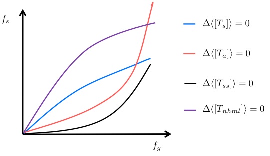
Figure 1: A cartoon of hypothetical isolines in the plane of greenhouse and solar forcings $f_{g}$–$f_{s}$ for various observables: globally averaged surface air temperature ($\Delta\langle[T_{s}]\rangle=0$), globally averaged atmospheric temperature ($\Delta\langle[T_{a}]\rangle=0$), averaged sea surface temperature ($\Delta\langle[T_{ss}]\rangle=0$), and surface air temperature averaged at the midlatitudes of the Northern hemisphere ($\Delta\langle[T_{nhml}]\rangle=0$). The diagram is a reproduction of Fig. 5 of Ref. Lucarini, 2013.

We point out that in the Planet Simulator intermediate-complexity GCM (PlaSim in short), Fraedrich (2012) the greenhouse and solar forcings have been found to be approximately equivalent in terms of the stationary response of the global average surface air temperature Boschi, Lucarini, and Pascale (2013) insomuch that its isolines are parallel straight lines (even if there is a curvature of the surface). This was found to be the case in rather extensive ranges of the forcings, 90–2880 ppm and 1200–1500 W m^-2, respectively. That is, any curvature of the blue line as shown in Fig. 1 occurs outside of the said ranges. However, in the context of geoengineering, the concern is whether these forcings are equivalent in the same sense in terms of other variables ($\Phi$) too, as discussed. We will demonstrate in PlaSim that with regard to regional averages $T_{s}$, the correspondence of forcings is still remarkable, but there is nevertheless a residual response with a nontrivial pattern under geoengineering. Furthermore, our analysis hints that (O2) this residual response might not be so linear, and less so for precipitation, which goes beyond the findings of MacMartin and Kravitz,MacMartin and Kravitz (2016) who demonstrate clearly the linearity only of the global average response under geoengineering, but average the linear predictions of spatial patterns over nine models. On the other hand, Cao et al. Cao et al. (2015) do indicate that the local response for several observables under geoengineering might be nonlinear by comparing the prediction of a linear regression model with simulation results for the HadCM3L model. However, we point out that it is possible that the local susceptibilities represented in the simple linear model were inaccurately estimated from model simulation data, and so further analysis would be needed to attribute the said mismatch to nonlinearity. This is what we attempt here.

This work follows Ragone et al. Ragone, Lucarini, and Lunkeit (2016) and Lucarini et al. Lucarini, Ragone, and Lunkeit (2017) The latter demonstrated that it is convenient for response theory to predict spatial patterns too, which, as outlined above, form the basis for one of the types of diagnostics that we pursue in order to assess the success of the geoengineering method. In both of these papers, the authors used PlaSim Fraedrich (2012) to demonstrate the power of their methodology, but with slightly differing setups of the model. Here we adopt the setup of Lucarini et al.Lucarini, Ragone, and Lunkeit (2017) featuring meridional ocean heat transport. The present work also builds on Gritsun and Lucarini Gritsun and Lucarini (2017) in adopting a simple technique to obtain a better estimate of the linear susceptibility, which was independently discovered by Liu et al. Liu et al. (2018) Clearly, a better susceptibility estimate would be useful in making a linear prediction only if the actual response were linear. Under [CO₂]-doubling, Ragone et al. Ragone, Lucarini, and Lunkeit (2016) and Lucarini et al. Lucarini, Ragone, and Lunkeit (2017) found a nonlinear response of the global average $\Delta\langle[T_{s}]\rangle$, and so no linear prediction would be productive in that case; however, under geoengineering, the total response is aimed to be much smaller, and so in principle the response may be linear. This is found to be approximately the case in PlaSim, and, so, as one of the main contributions of this work (O1), by improving the susceptibility estimates, we can improve greatly on our prediction of a solar forcing $f_{s}(t)$ required for cancellation, $\Delta\langle\Psi_{\varSigma}\rangle(t)=0$.

The structure of the remainder of this paper is as follows. Next, in Sec. II, we detail our methodology, listing a set of experiments performed to establish the response characteristics of the climate model and to assess nonlinearities, among other things. Then, in Sec. III, we provide results, first pertaining to objective (O1) about the success of the primary objective of geoengineering, namely, the cancellation (Sec. III.1.1), and then our diagnostics of other observables (Secs. III.1.2 and III.2). Finally, in Sec. IV, in terms of the stationary climate only (O1), we outline an improved method for obtaining the required solar forcing for cancellation, and also (O2) analyze our improved diagnostics with respect to the linearity of the response. In Sec. V we summarize our results and give our perspective for worthwhile future work. In a series of appendices we give details of the notation and algorithm for spectral analysis in discrete time (Appendix A), the way we obtain the Green’s functions (Appendix B), our novel solution method to the discrete- and finite-time inverse problem for a required solar forcing (Appendix C), and the circular convolution theorem (Appendix D), and we relegate the diagnostics of zonal averages to Appendix E.

II Methodology: Forcing scenarios

The form of the forcing signal $f_{g}$ due to changes in the carbon dioxide concentration $[{\rm CO}_{2}]$, for which we want to solve the geoengineering inverse problem, is a ramp that was used by Lucarini et al. Lucarini, Ragone, and Lunkeit (2017) This is a standard forcing type, also used for the CMIP6 DECK (Diagnostic, Evaluation and Characterization of Klima) protocols.Good et al. (2016) More precisely, it is not a time-continuous ramp, for the reason detailed in Appendix B, but $[{\rm CO}_{2}]$, and so $f_{g}$, is kept constant for one year after each incremental increase. The $[{\rm CO}_{2}][n+1]-[{\rm CO}_{2}][n]$ increment is a (small) fraction of the current value $[{\rm CO}_{2}][n]$, and therefore increasing in a superlinear fashion with time $[n]$, but, owing to the logarithmic dependence of the radiative forcing on the $[{\rm CO}_{2}]$ concentration,Huang and Bani Shahabadi (2014) it realizes a linear radiative forcing signal $f_{g}[n]$ (see Appendix A for the notation for a discrete time series), i.e., a constant-in-time ($n$) radiative forcing increment $f_{g}[n+1]-f_{g}[n]$. Hence the name “ramp.” Such a form of the forcing signal is useful in diagnosing or interpreting results. For example, if the response characteristic to solar forcing $f_{s}$ is similar to that of $f_{g}$, then the required solar forcing to cancel global change would also be approximately ramp-like.

Note, however, that a linearity of the response characteristic to any forcing is usually checked by a comparison of the linear prediction with the truth in terms of a model simulation subject to the same forcing. The latter we will refer to as “reference” in the following, instead of “truth.” Beside the nonlinearity, another factor that gives rise to a discrepancy is a statistical error due to the finite ensemble size. However, the latter has a very distinct feature that can be visually told apart easily from the contribution of nonlinearity. We reiterate that by applying a staircase-like forcing, we guarantee that the said discrepancy has no contribution due to calculations being performed in discrete time.

We point out that, at asymptotic times, there is no discrepancy at all, because of the way we estimate the Green’s function (Appendix B): the discrepancy emerges transiently only. Its all-time maximum is a useful intuitive measure of nonlinearity in the examined regime. In any case, the larger the response, the greater is the nonlinear contribution to it, and so—in the context of system identification—the more inaccurate our estimates of the susceptibilities (Appendix B) become. Therefore, beside our base scenario of (overall) doubling $[{\rm CO}_{2}]$, we will also check if we can obtain a more accurate (and so useful for the geoengineering problem) estimate of the Green’s function using a weaker identification forcing. In particular, we apply a $[{\rm CO}_{2}]$ change that results in half of the (overall) radiative forcing change of that by doubling $[{\rm CO}_{2}]$. (This is realized by $[{\rm CO}_{2}]_{\infty}/[{\rm CO}_{2}]_{0}=\sqrt{2}$, according to the above-mentioned logarithmic law.Huang and Bani Shahabadi (2014)) Note that in the case of this weaker forcing, irrespective of the different plateau level, the increments of the $[{\rm CO}_{2}]$ changes realize the same 1%/yr relative change.

We refer the reader to Table 1 for an overview of the various identification and test forcing scenarios that we used in the present study. Among them, we have CQ2 defined by 0.1%/yr relative changes, which makes it a much slower change than the base scenario. The response to such a slow ramp forcing should be ramp-like as long as the linear term in Eq. (2) dominates over the nonlinear ones. This forcing scenario will therefore provide us another reference in interpreting other results with respect to linearity.

In Table 1, we have not indicated the plateau level of the solar forcing $f_{s}$ used in conjunction with $f_{g}$. We chose this level such that the response asymptotically in terms of the global average surface air temperature is the same but of opposite sign as that due to the corresponding $f_{g}$. This level can be easily determined to a good approximation by an iterative procedure. Beside those in Table 1, we will introduce a few more forcing scenarios in Sec. IV: some forcing scenarios that will give improved results, and other forcing scenarios that aid the interpretation of our results. The abrupt stepwise forcing scenarios, CS1, SS1, CS2, SS2, are employed to numerically determine the Green’s functions as detailed in Appendix B.

Table 1: Sets of simulation data specified by the forcing. Each data set is codenamed by a three-character code, the first character coding the quantity in which the forcing is presented (C for $[{\rm CO}_{2}]$ and S for solar irradiance), the second character coding the “form” of the forcing signal (S for step, R for ramp, and Q for slow ramp), and the third character coding the plateau level of the (corresponding—see text) greenhouse forcing (2 for $[{\rm CO}_{2}]_{\infty}/[{\rm CO}_{2}]_{0}=2$ and 1 for $[{\rm CO}_{2}]_{\infty}/[{\rm CO}_{2}]_{0}=\sqrt{2}$). The CS2 and CR2 data sets are preexisting to the present study,Lucarini, Ragone, and Lunkeit (2017) consisting of 200 ensemble members. All new data sets listed here consist of 20 ensemble members each, except for CQ2, which consists of 10.

	Form:	Step		Ramp		Slow ramp
Forcing	Plateau:	$2$	$\sqrt{2}$	2	$\sqrt{2}$	2
$[{\rm CO}_{2}]$		CS2	CS1	CR2	CR1	CQ2
Solar		SS2	SS1	SR2	SR1
Combined				BR2	BR1

III Results

III.1 Surface air temperature

III.1.1 Global average

The global average surface air temperature is the variable with respect to which we prescribe the cancellation. We do not consider any other variable in this role throughout the present study. Having predicted the solar forcings (SR1, SR2) required to produce no total response used in combination with prescribed $[{\rm CO}_{2}]$ forcings (CR1, CR2) adopting the methodology described in Appendix C, we plot the predicted linear responses in Fig. 2(a). Clearly, these predictions can be viewed either as components of the predicted total response (BR1, BR2), or the predicted response in separate scenarios (CR1, CR2, SR1, SR2). Alongside these predictions, we plot the true response in the scenarios when the forcings are applied separately, i.e., the responses evaluated by direct numerical simulations (CR1, CR2, SR1, SR2). The comparison of prediction and reference reveals that (i) the response to stronger forcing is more nonlinear in the case of greenhouse forcing (CR2) in comparison with solar forcing (SR2) and (ii) with a weaker identification (CS1, SS1) and test forcing (CR1, SR1), the linear prediction for CR1 is much better than that for CR2, while SR1 is seemingly as good as SR2. For the scenarios of combined forcing (BR1, BR2), only the true response is nontrivial if nonlinear, which is displayed in Fig. 2(b). Indeed, because of the nonlinearity, the total asymptotic response is nonzero. (Note that the fluctuations at asymptotic time are due to the finite ensemble size.) It is visibly nonzero even with the weaker forcings. However, it is just about 10% of that with greenhouse forcing solely, even in the case of the stronger forcings.

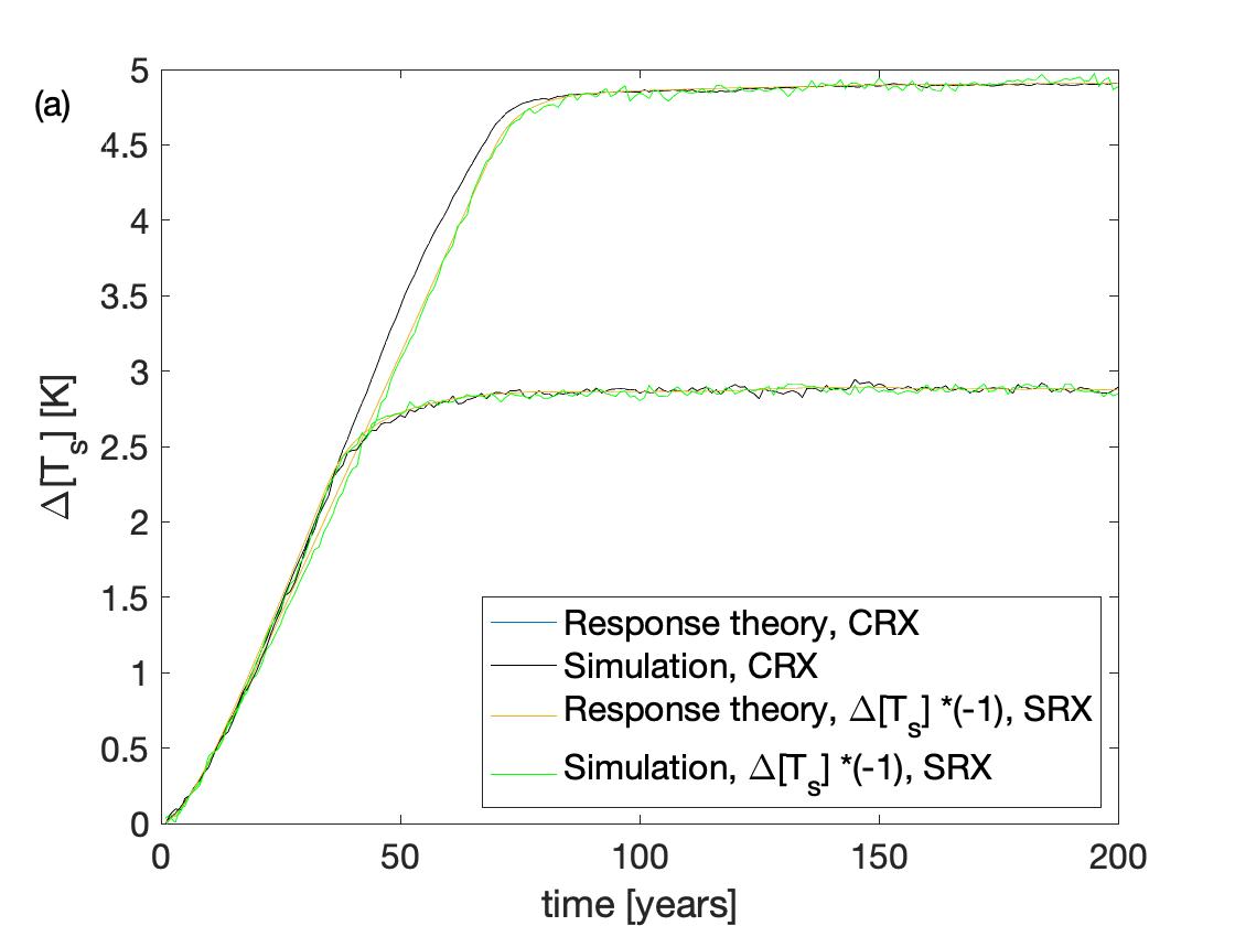
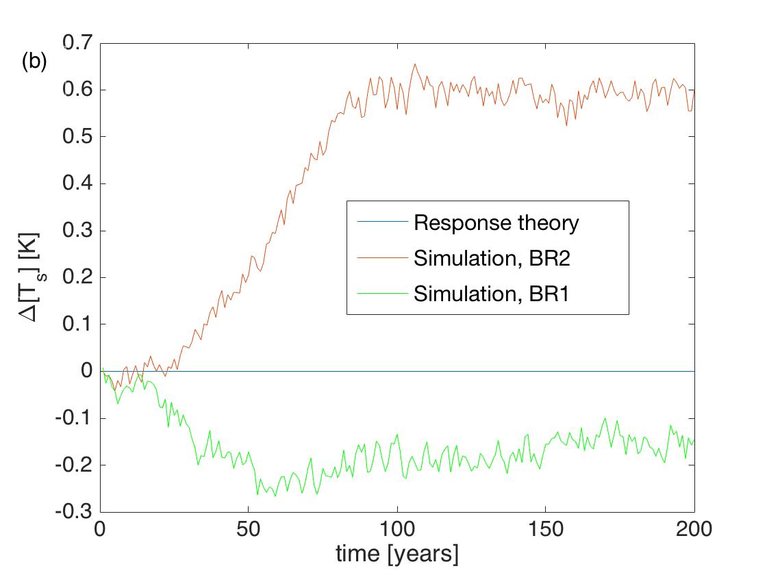
Figure 2: Predicted and true surface air temperature responses to ramp-like forcings. Forcing scenarios are (a) CR1, CR2, SR1, SR2 and (b) BR1, BR2. Note that in the keys, e.g. in “CRX”, “X” can stand for either “1” or “2”, and, intuitively, these scenarios can be told apart in the diagram by the greater/smaller response levels. Note also that in (a), the two yellow curves perfectly cover the corresponding light blue ones, because $f_{s}$ is calculated to cancel global warming at all times.

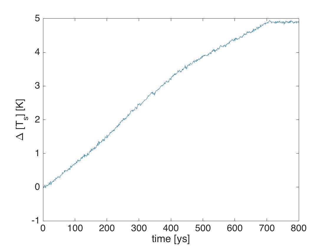
Figure 3: True response of the global mean surface temperature under a very slow ramp forcing, CQ2.

The pronounced nonlinearity [point (i) above] shows up also in other experiments. With a very slow forcing CQ2, we registered the response as shown in Fig. 3. Although the rate of forcing is unchanged throughout the time period of almost 700 years, the response switches to a slower rate between 400 and 500 years, or, between 3 and 4 K changes in the temperature. The placement of this change in the rate, compared with the asymptotic temperature change of almost 3 K upon the weaker CR1 forcing seen in Fig. 2(a), is in good agreement with the observation of a much more closely linear response to that weaker forcing as compared with CR2. A crude indicator of non/linearity can be extracted from the CQ2 experiment, but also from comparing the asymptotic/stationary responses (denoted by a subscript $\infty$) in the XX1 and XX2 experiments, as the following ratio:

$$\rho=\frac{{\Delta\langle[T_{s}]_{\infty,2}\rangle}/{\Delta\langle[T_{s}]_{\infty,1}\rangle}}{{f_{\infty,2}}/{f_{\infty,1}}}=\frac{{\Delta\langle[T_{s}]_{\infty,2}\rangle}/{f_{\infty,2}}}{{\Delta\langle[T_{s}]_{\infty,1}\rangle}/{f_{\infty,1}}}.$$ (14)

(Note that we write an “X” in place of one of the possible characters in the scenario identification code when it does not matter which of the possible characters is written there.) This value is $\rho=0.99$ with solar forcing and 0.85 with greenhouse forcing, in agreement with what the comparison of predicted and true responses, seen in Fig. 2(a), allowed us to conclude above.

III.1.2 Spatial pattern

We continue with the diagnostics of the geoengineering method in view of uncontrolled observables. We begin by looking at the observable of the same physical quantity, the surface air temperature, but of a spatial scale other than the global average. We would like to map out the spatial variation of the total response. A comprehensive view of the spatial variations of the response is given by the distribution over the 2D surface, computing the response at each gridpoint separately, as done by Lucarini et al. Lucarini, Ragone, and Lunkeit (2017) Similarly to zonal averages (Appendix E), the response patterns to greenhouse and solar forcings are very similar in the stationary climate regimes; see Figs. 4(a) and 4(b) for the strong forcings CR2 and SR2, respectively. (See Ref. Hansen et al., 2005 for such a comparison in a complex model.) The patterns in Figs. 4(a) and 4(b) are misaligned slightly, which results in nonzero predicted total responses (BR2) of opposite sign in neighboring regions. This is shown in Fig. 4(c). The picture for the weaker forcings, CR1, SR1 (not shown), and BR1 [Fig. 4(e)], is similar.

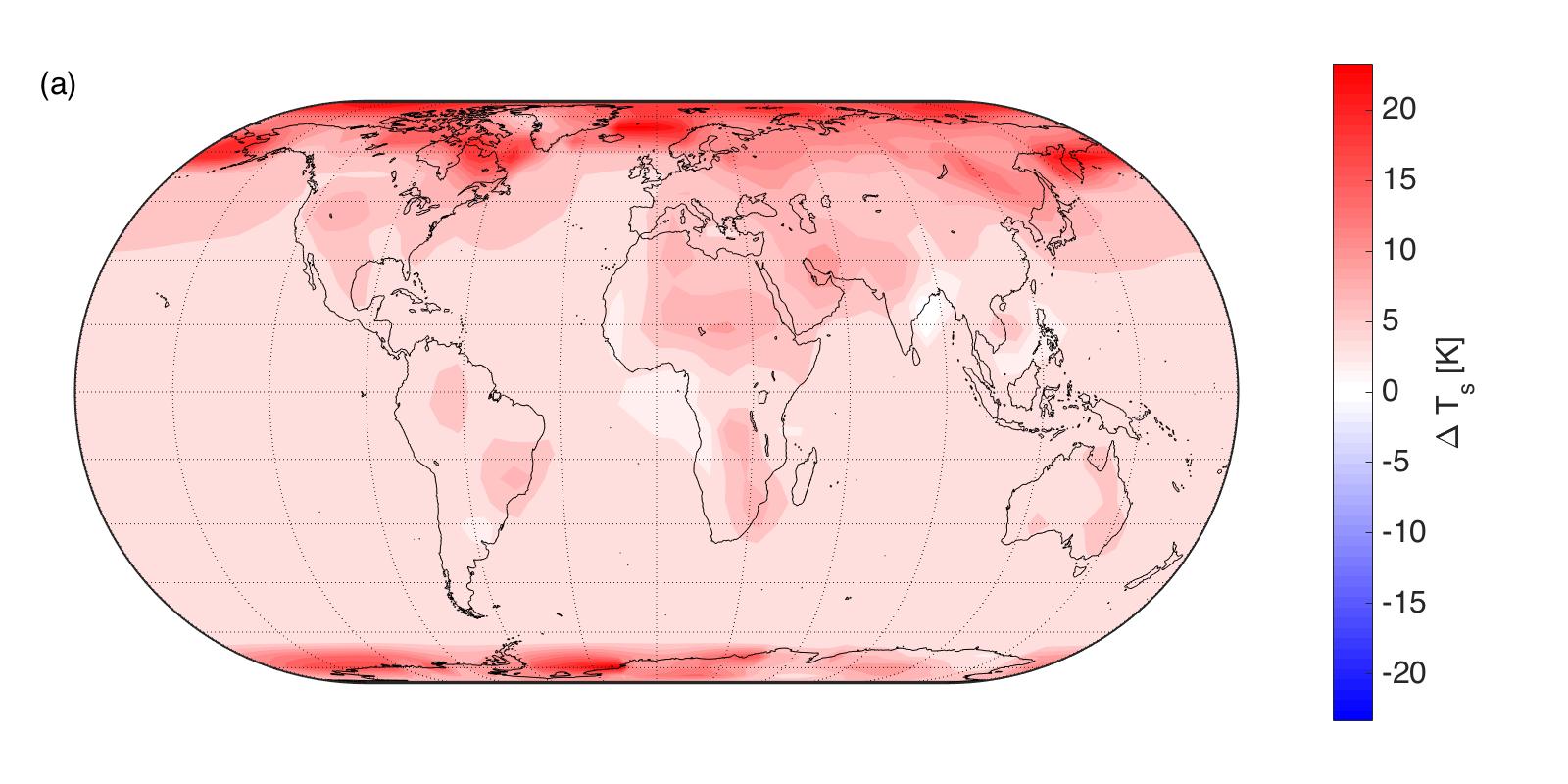
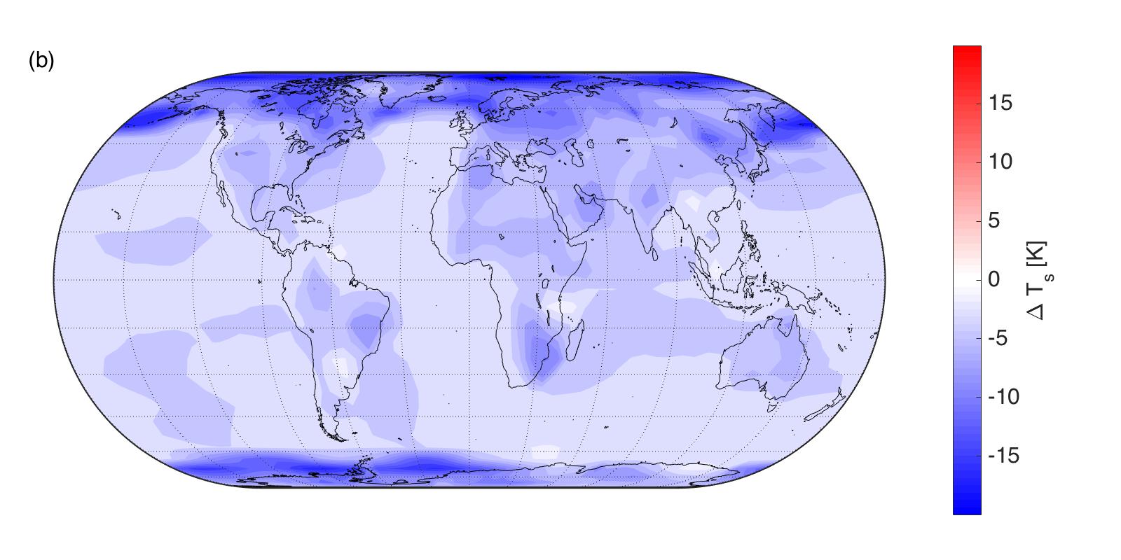
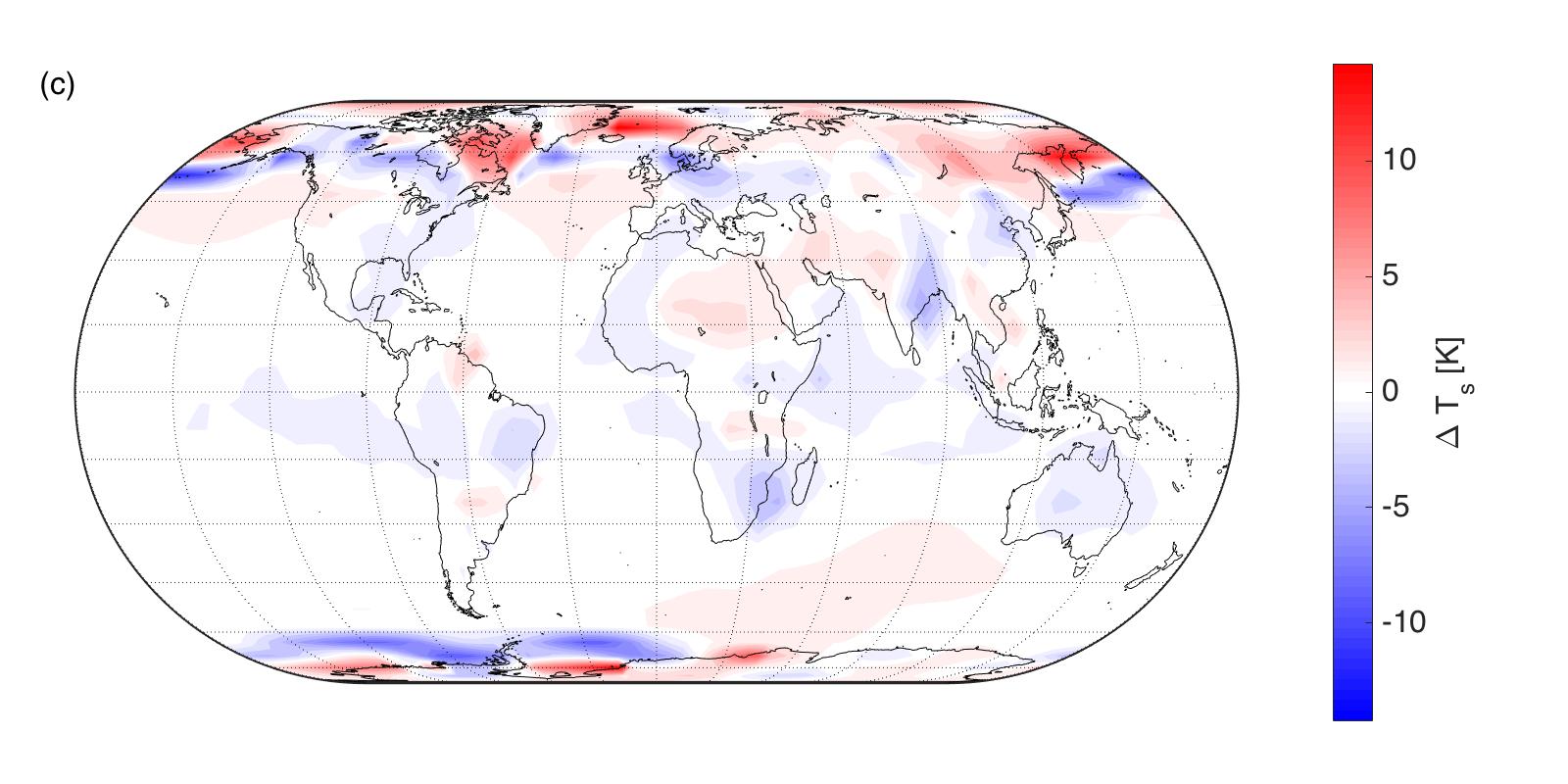
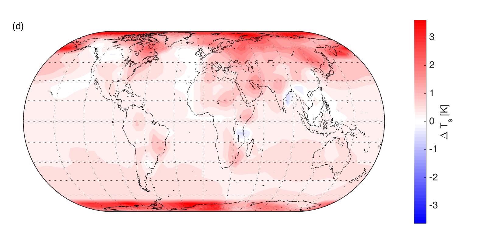
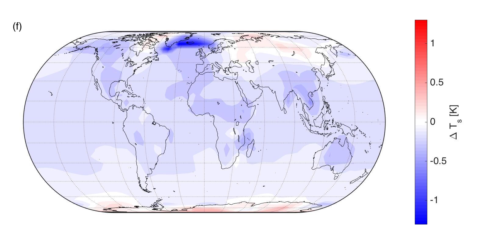
Figure 4: Spatial variation of the stationary climate in terms of the surface air temperature belonging to different forcing levels specified by plateaus of forcings collected in Table 1: (a) CX2; (b) SX2; (c) BX2; (d) BX2; (e) BX1; (f) BX1. All diagrams picture the reference, except for (c) and (e), which show the linear predictions. Note the different ranges of the temperature for the color bars.

Unsurprisingly, large predicted residual total responses occur where the response is large to either greenhouse or solar forcing alone. However, the predicted total response turns out to be grossly erroneous; the reference regarding the surface air temperature, shown in Figs. 4(d) for BR2 and 4(f) for BR1, shows that significant cancellation is achieved even locally. [We note that the overwhelmingly red and blue colors in Figs. 4(d) and 4(f), respectively, are consistent with the signs of the true residual total global change shown in Fig. 2(b).] However, looking at the temperatures at the highest model level, nearest the tropopause, the response under combined forcing [BX2, Fig. 5(a)] is comparable in magnitude to the response under, say, solar forcing alone [SX2, Fig. 5(b)]—nothing like the situation on the surface as seen in Figs. 4(b) and 4(f).

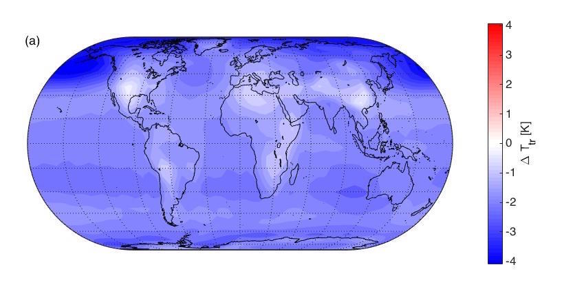
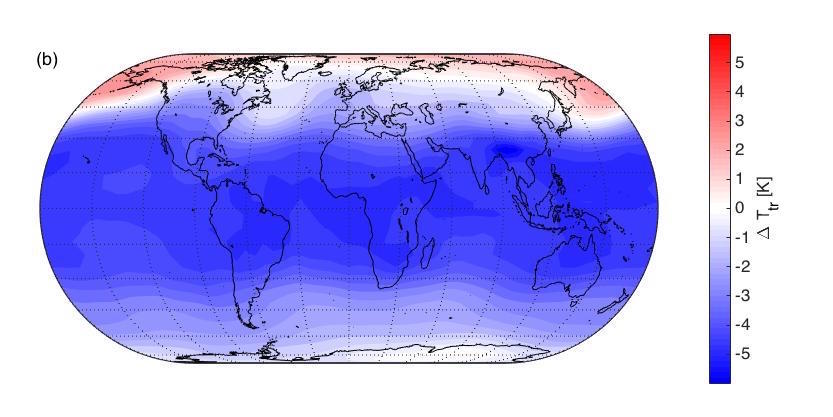
Figure 5: True spatial variation of the stationary climate in terms of the air temperature in the topmost model layer, nearest to the tropopause: (a) BX2; (b) SX2.

III.2 Annual precipitation

Here we present results for another diagnostic observable, the annual precipitation $P_{y}$. In terms of the spatial patterns of the response, very similar conclusions can be drawn for the precipitation as for the surface air temperature, and these conclusions are supported by the set of diagrams in Fig. 6. The difference is that the largest responses are observed at equatorial regions, and it is not clear what mechanism causes this. Most importantly, significant cancellation is actually achieved as opposed to the much less favorable linear prediction. This is so even if the solar forcing used is the same as before, i.e., one determined with the aim of canceling global warming (not wettening; in the same spirit as Fig. 4 of Ref. MacMartin and Kravitz, 2016). The significant cancellation clearly suggests that the response characteristics of $P_{y}$ to greenhouse and to solar forcing, say in terms of the respective Green’s functions, are very similar, as with the corresponding Green’s functions of $T_{s}$. Nevertheless, there are differences too, as seen in Fig. 7, such as the more obvious nonmonotonicity of the evolution, despite a monotonic forcing. Furthermore, the linear prediction for the total response in the stationary climate is nonzero, which is clearly because we are looking at an uncontrolled observable. This linear prediction, however, is quite “unreliable,” as can be expected from the mismatch of the true and predicted spatial patterns. Otherwise, both the predicted and the true total global mean responses to combined forcing look rather negligible compared with the responses to the greenhouse or solar forcings acting separately; see also Table 2. Interestingly, the transient responses (not shown) have similar qualities to those of the temperature: nonlinearity is most obvious for CR2 as opposed to CR1, SR1, and SR2.

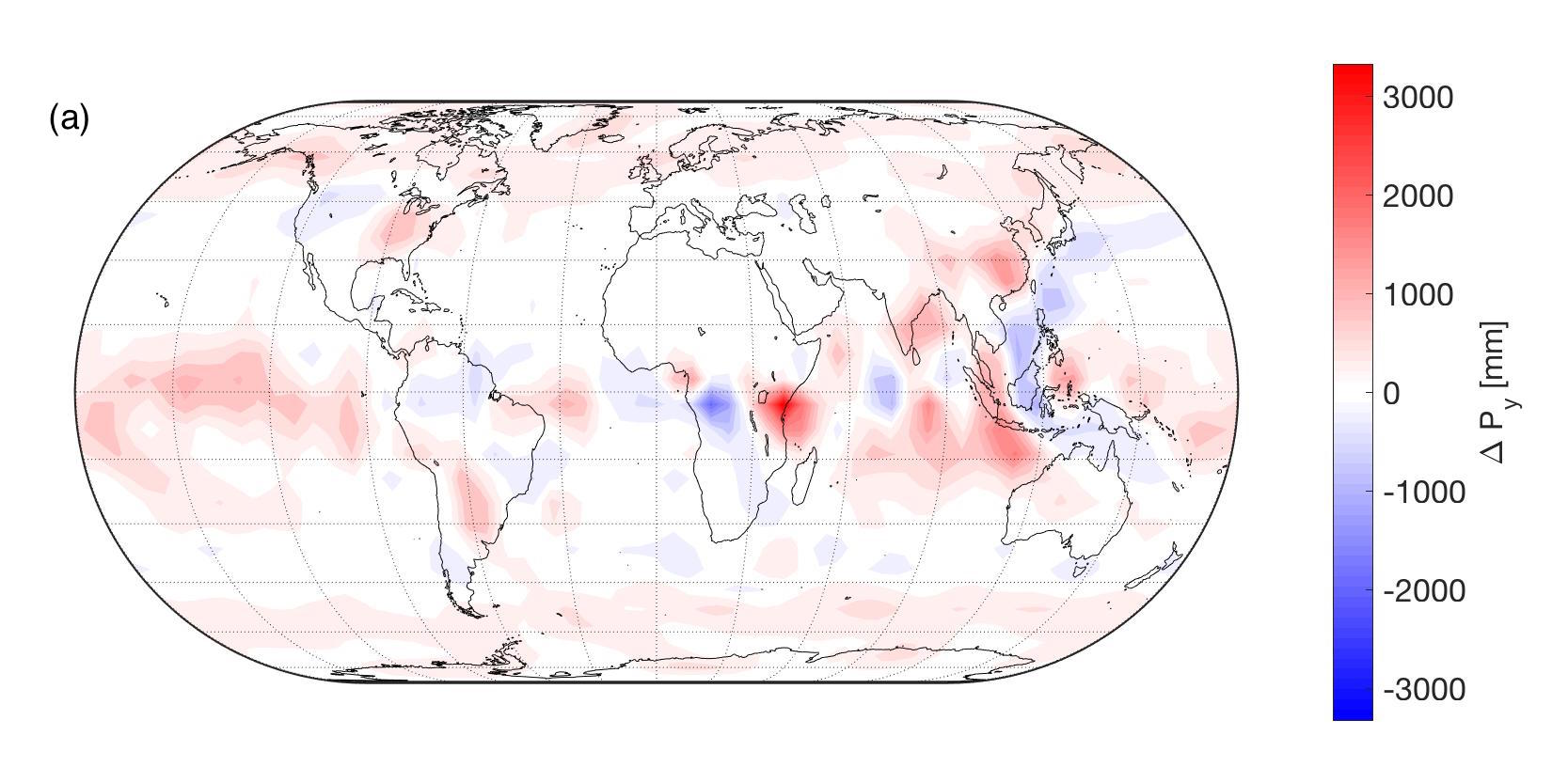
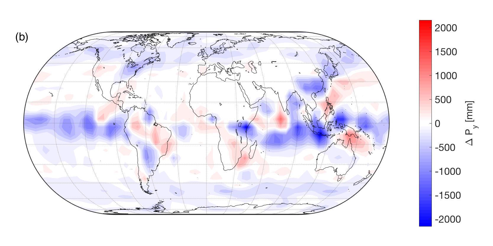
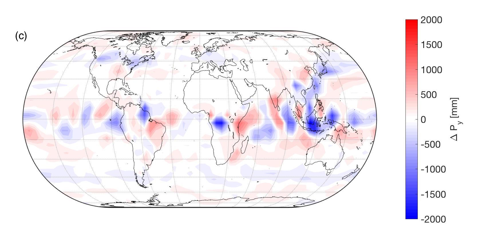
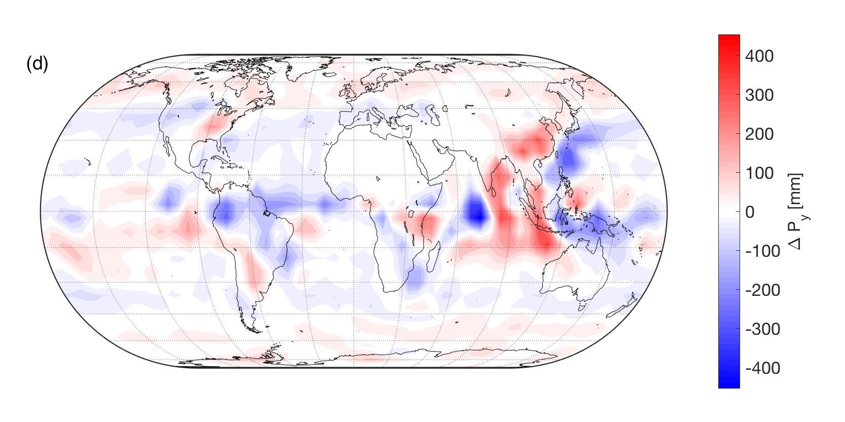
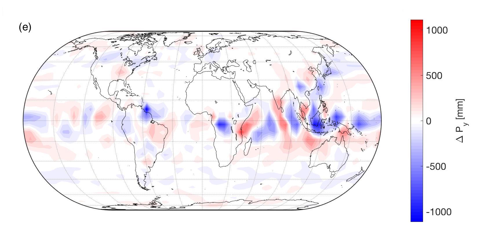
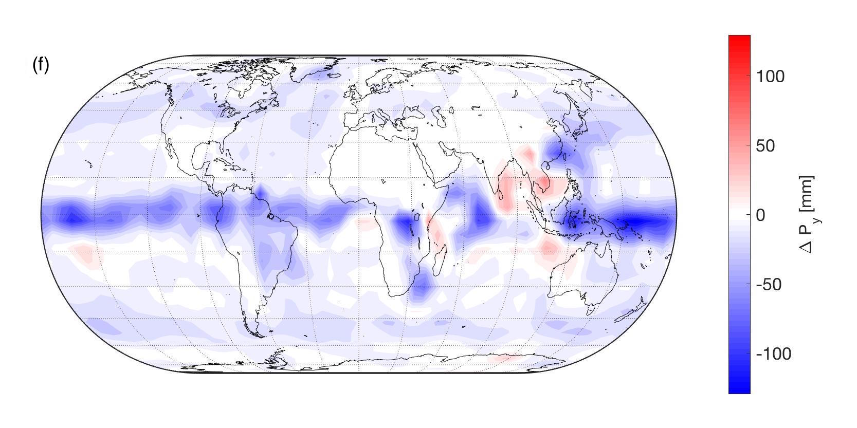
Figure 6: Same as Fig. 4, but for the annual precipitation.

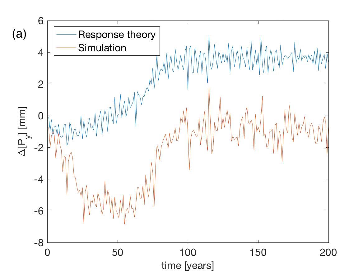
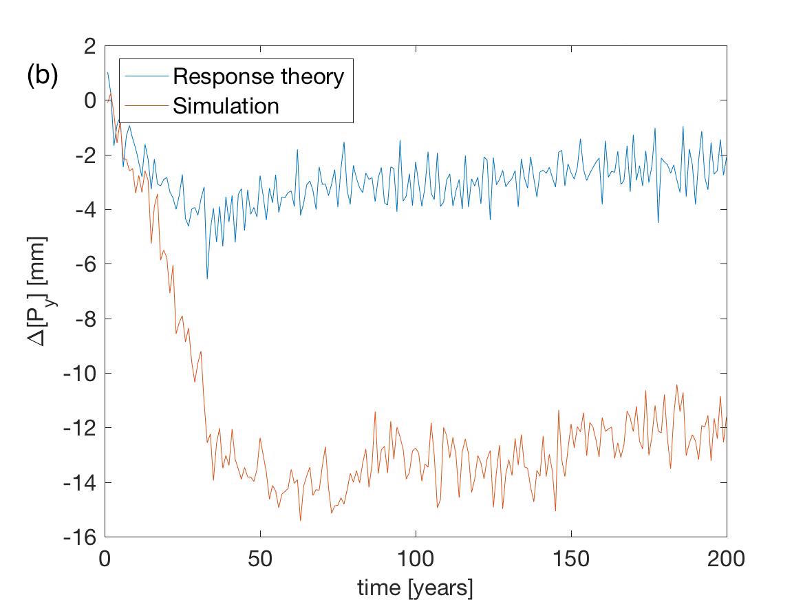
Figure 7: Same as Fig. 2(b), but for the annual precipitation and showing separately the cases of (a) BR2 and (b) BR1.

Table 2: Global average stationary climatology of the annual precipitation belonging to different forcing levels.

Forcing	CX1	CX2	SX1	SX2
$\Delta\langle[P_{y}]\rangle_{\infty}$ (mm)	74	124	$-$71	$-$121

We note that equatorial drying under a similar geoengineering scenario has also been reported by others.Ferraro, Highwood, and Charlton-Perez (2014); MacMartin and Kravitz (2016) However, in these studies a quadrupling of [CO₂] was considered. We point out that it does seem to matter what levels of change we consider: under [CO₂]-doubling, we actually find less drying than in the case of the $\sqrt{2}$-fold [CO₂] increase. This finding can, however, have different reasons. One candidate is that the response under combined forcing is nonlinear; another is that (assuming that the response under combined forcing is approximately linear) the required solar forcing was determined inaccurately [which already resulted in a residual response as seen in Fig. 2(b)]. Note that in Refs. Ferraro, Highwood, and Charlton-Perez, 2014; MacMartin and Kravitz, 2016, an exact cancellation of global mean surface temperature was achieved in the stationary climate, like, for example, in the G1 GeoMIP experiment. Given this, Fig. 4 of Ref. MacMartin and Kravitz, 2016 indicates that the response of the global mean is approximately linear in most CMIP5 models considered, at least up to a certain forcing level that was actually lower than [CO₂]-doubling. In the following, we indicate that both of the said effects play a role, i.e., nonlinearity is likely also present in our case; however, it might not be the dominant component. Drying while global average surface temperature was maintained in a model was reported also by Ricke et al. Ricke, Morgan, and Allen (2010); Ricke et al. (2012)

IV Improved methodology and results

IV.1 Achieving a cancellation of the global mean surface temperature change

This subsection pertains to our objective (O1). The very close resemblance of the patterns seen in Figs. 4(a) and 4(b) hints that the effect of a changing $[{\rm CO}_{2}]$ on the radiative forcing shaping the surface air temperature is very similar to that due to a changing solar strength. However, with these data, we are not properly informed about just how similar, because, for example, the CR2 and SR2 forcings act in opposite directions and, owing to nonlinearities, they do not have to have the same effect even if the effects due to forcings acting in the same direction are indistinguishable. Therefore, we produced just that missing simulation: complementing SS2, for which the applied solar forcing is a step of equal magnitude but opposite sign. For this forcing, the stationary climate is shown in Fig. 8(a), to be referred to as SS2I. It is virtually indistinguishable from the pattern resulting for CS2, seen in Fig. 4(a), including a lack of such misalignment as the comparison of Figs. 4(a) and 4(b) revealed. This goes beyond the report on the (approximate) “equivalence” of greenhouse and solar forcings with respect to (asymptotic in time) global average surface temperature;Boschi, Lucarini, and Pascale (2013) this is extended now to regional averages, i.e., spatial patterns, of that variable with a remarkable degree of approximation. [Just how close this equivalence is will be indicated by Fig. 9(a).]

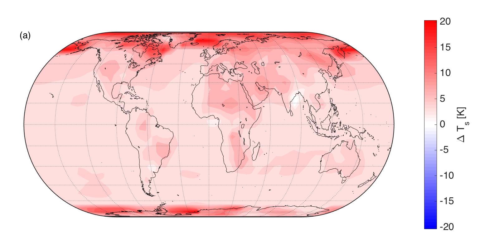
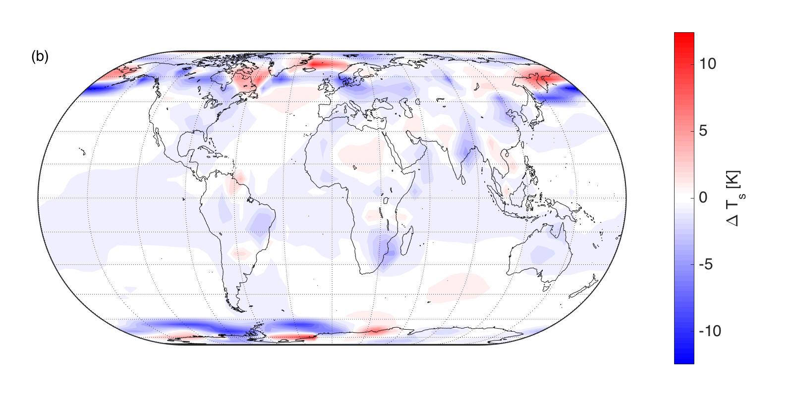
Figure 8: Spatial variation of the stationary climate in terms of the air temperature: (a) true response under SS2I; (b) predicted response under combined forcings used for SS2 and SS2I amounting to no forcing.

The superposition of the stationary climates for SS2 and SS2I, displayed in Fig. 8(b), is in turn almost indistinguishable from the asymptotic total response to combined BR2 forcing, seen in Fig. 4(c). By inspection of Eq. (2), this pattern turns out to be created by even-order nonlinear perturbative terms of the response. The selection of the even-order terms takes exactly the superposition of the responses from two experiments where the forcings are equal but of opposite sign: $\varepsilon_{1}=-\varepsilon_{2}$.

Instead of eliminating the even-order terms by superposition, we can retain only the odd-order terms by subtraction. We proceed in this direction, assuming that the third-order and higher odd-order terms make a negligible contribution. This way, we attempt to improve on the results for the linear susceptibility—and so ultimately on our prediction of the required solar forcing needed for canceling global warming. This is done with the aim of making an advance regarding our objective (O1). We can then apply this forcing in a new experiment coded as BR2C (“C” for “cancel”). For this experiment, we can utilize (although we will not examine the transient) our finding that the response characteristics to greenhouse and solar, i.e., short-wave and long-wave radiative, forcings are very similar, which would allow the application of a solar forcing that is a simple straight ramp, just like $\log([{\rm CO}_{2}]/[{\rm CO}_{2}]_{0})(t)$, having the same length before the plateau. (This should be the rationale behind the G2 experiments of GeoMIP.) That is, what we improve on here is only the level of the plateau. It is rather straightforward to obtain the following equations for this level $f_{\infty,BR2C,s}$:

$$\chi_{[T_{s}],\infty,s} =\frac{|\Delta\langle[T_{s}]\rangle_{\infty,SS2}|+|\Delta\langle[T_{s}]\rangle_{\infty,SS2I}|}{2|f_{\infty,SS2}|},$$ (15)

$$\chi_{[T_{s}],\infty,g} =\frac{|\Delta\langle[T_{s}]\rangle_{\infty,CS2}|+|\Delta\langle[T_{s}]\rangle_{\infty,CS2I}|}{2|f_{\infty,CS2}|},$$ (16)

$$|\Delta\langle[T_{s}]\rangle_{\infty,BR2C}| =\chi_{[T_{s}],\infty,s}|f_{\infty,BR2C,s}|-\chi_{[T_{s}],\infty,g}|f_{\infty,BR2C,g}|,$$ (17)

$$|\Delta\langle[T_{s}]\rangle_{\infty,BR2C}| =0.$$ (18)

The subscripts $\infty$ refer to the asymptotic, stationary climate regime; other subscripts refer to the experiment, i.e., forcing scenario. Observe that we need data from a new experiment, CS2I, where the “I” indicates an experiment related to CS2 analogously to the relation of SS2I to SS2. Since we are interested in the stationary climate regime only, owing to ergodicity we can produce just a single long trajectory instead of an ensemble. The result of this is $\Delta\langle[T_{s}]\rangle_{\infty,CS2I}=-5.11$ K (while we already have $\Delta\langle[T_{s}]\rangle_{\infty,SS2I}=4.36$ K, and, from Fig. 11, $\Delta\langle[T_{s}]\rangle_{\infty,SS2}=-\Delta\langle[T_{s}]\rangle_{\infty,CS2}=-4.90$ K). Having $|f_{\infty,BR2C,g}|=|f_{\infty,CS2}|$, we can express the sought-for forcing in relative terms based on the temperature data only, such as

$$\frac{|f_{\infty,BR2C,s}|}{|f_{\infty,SS2}|}=\frac{|\Delta\langle[T_{s}]\rangle_{\infty,CS2}|+|\Delta\langle[T_{s}]\rangle_{\infty,CS2I}|}{|\Delta\langle[T_{s}]\rangle_{\infty,SS2}|+|\Delta\langle[T_{s}]\rangle_{\infty,SS2I}|}=1.08.$$ (19)

In fact, we carried out the BR2C experiment independently: iteratively determining a solar forcing that cancels to a very good approximation the total response (similarly to how the level for, e.g., SS2 was determined observing the result of CS2). This forcing in the above relative terms was found to be 1.11, agreeing well with our prediction of 1.08.

Given that our prediction is smaller than the forcing actually needed for cancellation, we can predict an upper bound on the actual total response to our predicted forcing by substituting the actually needed value $|f_{\infty,BR2C,s}|/|f_{\infty,SS2}|=1.11$ into Eq. (17) (assuming that the response under combined forcing is linear). This gives $\Delta\langle[T_{s}]\rangle_{\infty,BR2C}<0.134$ K. Considering that the total residual response with the original naive methodology (Appendices B and C) was 0.6 K, this means that with the improved methodology we managed to reduce the total response almost to one-fifth or even less of the said first result. (Of course, the exact reduction can be easily determined by an extra simulation, which we have not run.) In fact, some residual total response even with the improved method could be expected, since the simple measure of nonlinearity (14) indicated that linearity is much more violated by an increasing radiative forcing as opposed to a decreasing one. This suggests that the third-order odd perturbative term is not very small relative to the second-order one—contrary to the assumption of our improved methodology. Another source of error could be a nonlinear component of the response under combined forcing. This is what we examine next.

IV.2 Uncontrolled response and its (non)linearity

This subsection pertains to our objective (O2). Even if we managed to achieve a perfect cancellation in terms of the global averages, amounting to a success in terms of our objective (O1), it is still important to examine the total response in terms of any other observables regarding which the cancellation is not enforced, to see whether there is any unwanted residual. To this end, we look at the BR2C data. In particular, in Fig. 9, we show the spatial variations of the stationary climate in terms of (a) the surface air temperature and (b) the annual precipitation. The former looks to be a result of interpolating between the maps of Figs. 4(d) and 4(f), and the latter looks to have the same relationship with the maps seen in Figs. 6(d) and 6(f). This implies that the variances with respect to space for BR2C (exact cancellation), both for temperature and for precipitation, are about the same as those for BR2 (approximate cancellation employing a naive method), and are much larger than the residual total responses in terms of the respective global averages for BR2. The reason for this must be that typically the respective (not necessarily linear) local response characteristics to greenhouse and solar forcing are somewhat different. Furthermore, comparing the BR2 and BR2C scenarios, we see that the difference in terms of the climatic surface air temperature could be as much as 2 K, which is about 10% of the maximum response under the corresponding greenhouse forcing alone. This justifies very well the application of the improved methodology as described in Sec. IV.1. We note that the cooling tropics and warming arctic under global average surface temperature cancellation are in agreement with the findings of other studies using state-of-the-art models, including the first study examining the side-effects of geoengineering by Govindasamy and Caldeira. Govindasamy and Caldeira (2000)

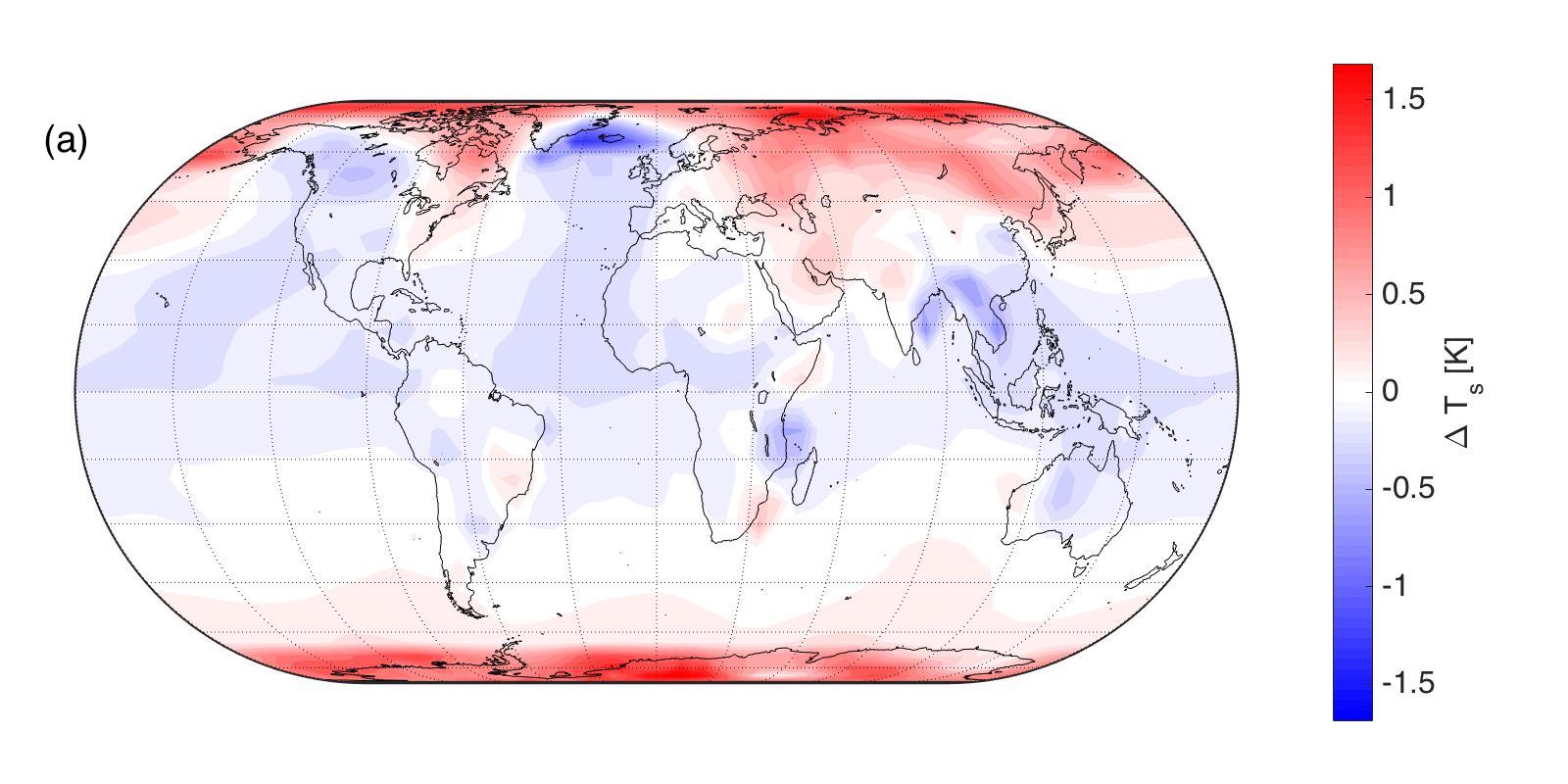
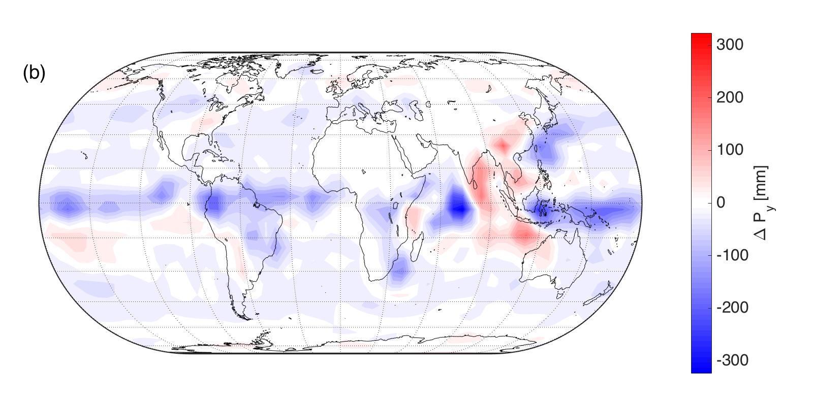
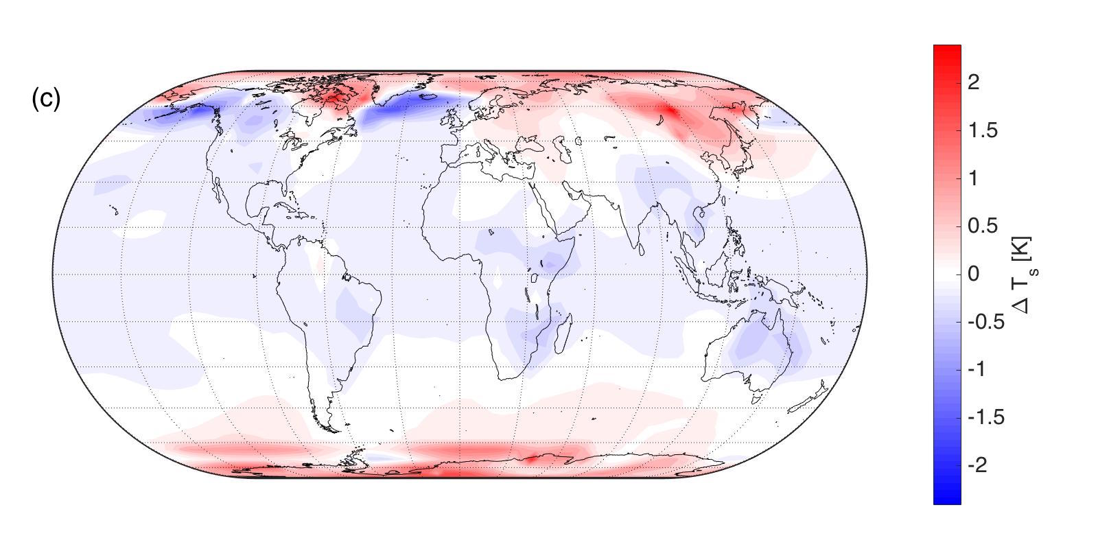
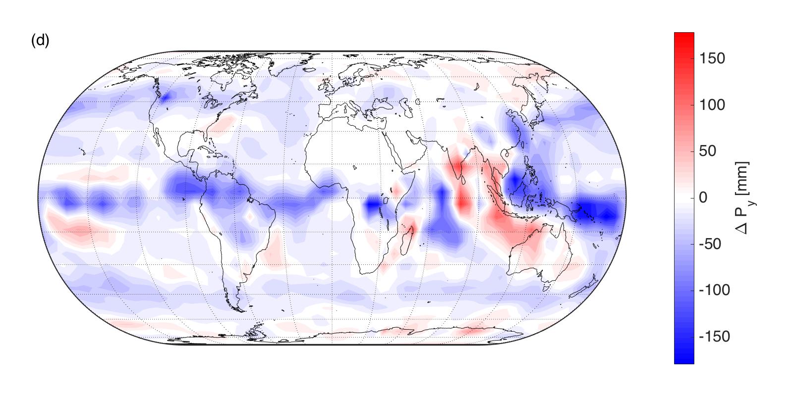
Figure 9: Spatial variation of the stationary climate in terms of (a) the surface air temperature and (b) the annual precipitation in the BR2C experiment, when a change in the global average surface air temperature is canceled. (c)/(d) The improved linear prediction corresponding to (a)/(b).

The improved methodology to estimate susceptibilities applies of course to regional averages too. What remains to be seen now is whether linear response theory can predict the residual total responses seen in Figs. 9 (a) and 9(b) (O2). The corresponding linear predictions are shown in Figs. 9(c) and 9(d), respectively. These predictions show a dramatic improvement on the first results shown in Figs. 4(d) and Fig. 6(d), respectively. Quantitatively, however, the prediction is not perfect. We can quantify this by, for example, the Pearson correlation coefficient $C$ between the reference $\Delta\langle\Psi\rangle$ and the linear prediction $\langle\Psi\rangle^{(1)}$, the results for which are shown in Table 3. (Note that no weighting of the data points with the area represented by gridpoints is done.) This shows that the prediction skill is better for the temperature than the precipitation.

Table 3: Measures of overall nonlinearity of the response in terms of the local temperature and precipitation. $C$ is the Pearson correlation coefficient between the reference $\Delta\langle\Psi\rangle$ and the linear prediction $\langle\Psi\rangle^{(1)}$, and $\rho$ is defined by Eq. (21). Note that to calculate std($\rho$), values of $\rho$ larger in modulus than 5 are discarded. The last column is devoted to the global averages.

	Pearson correlation coefficient	std($\rho$)	$\rho$
$T_{s}$	0.78	0.26	0.73
$P_{y}$	0.53	1.01	0.70

Whether the imperfection of the linear prediction is due to nonlinearity—as a small error $E=\Delta\langle\Psi\rangle-\langle\Psi\rangle^{(1)}$ would normally suggest—is not clear, because it is possible that the response $\Delta\langle\Psi\rangle$ is linear but errors in the susceptibility estimates determining $\langle\Psi\rangle^{(1)}$ (or rather its estimator) remain. We should therefore find a way to check linearity without relying on the linear prediction. This can be done in a naive way similarly to what we did for single-forcing scenarios, evaluating $\rho$ as defined by Eq. (14). However, this time, we have not one but two forcings present. Because of this, it turns out that a check of linearity requires not two but three data points at least. In fact, we are readily endowed by three data set candidates resulting from the BR1, BR2, and BR2C experiments. In each scenario, if the response is linear, the asymptotic climate would be given by an equation like

$$\Delta\langle\Psi_{i}\rangle=\chi_{\Psi,g}f_{i,g}+\chi_{\Psi,s}f_{i,s},\qquad i=1,2,3,$$ (20)

where $i=1,2,3$ stand for, say, BR1, BR2, BR2C, in that order. One can express $\chi_{\Psi,s}$ from the equation for $i=3$, substitute into the equations for $i=1,2$, and from these latter express $\chi_{\Psi,g}$. Under linearity, the ratio of these expressions,

$$\rho=\frac{\quad\dfrac{\Delta\langle\Psi_{2}\rangle-\Delta\langle\Psi_{3}\rangle\frac{f_{2,s}}{f_{3,s}}}{f_{2,g}-f_{3,g}\frac{f_{2,s}}{f_{3,s}}}\quad}{\quad\dfrac{\Delta\langle\Psi_{1}\rangle-\Delta\langle\Psi_{3}\rangle\frac{f_{1,s}}{f_{3,s}}}{f_{1,g}-f_{3,g}\frac{f_{1,s}}{f_{3,s}}}\quad},$$ (21)

would be unity, meaning that Eqs. (20) are in fact satisfied. We have evaluated $\rho$ for all gridpoints and display the results in Fig. 10. This suggests that we do have nonlinearity for both the temperature and precipitation. However, this conclusion can be called into question by noticing that the three data points could be too close to one another, resulting possibly in an inaccurate estimation of the ratio $\rho$, thereby falsely suggesting nonlinearity. Instead of evaluating $\rho$, faced with finite data set size to evaluate climatic means, a test statistic would be a proper way of indicating nonlinearity at individual gridpoints. Gottwald, Wormell, and Wouters (2016) Nevertheless, based on the available data still, one idea to indicate that deviations from unity of both the correlation coefficient $C$ and $\rho$ are due to nonlinearity would be to demonstrate a correlation between the local errors $E$ of the linear prediction and $\rho$. We have checked the scatterplots of these quantities for both the temperature and precipitation and found no sign of correlations. This, however, does not mean that the response is linear: some unidentified effect could destroy the correlation. Our final idea is that if two situations feature different levels of nonlinearity, even if the two gridpoint-wise quantifiers of nonlinearity, $E$ and $\rho$, have random errors, typically they should indicate in a coordinated way a stronger deviation from linearity in the case when nonlinearity is actually stronger. We propose to capture this typical behavior by the correlation coefficient $C$ on the one hand, and the standard deviation std($\rho$) over the gridpoints on the other. We note that even if linearity is typical, a smaller std($\rho$) would indicate that it is more typical. We have already given the correlation coefficient in Table 3, where we also display std($\rho$). We do indeed see that both quantities suggest that the response of precipitation is more nonlinear.

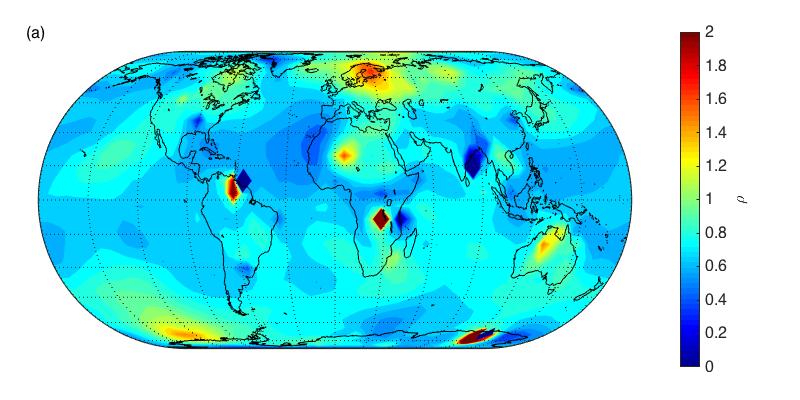
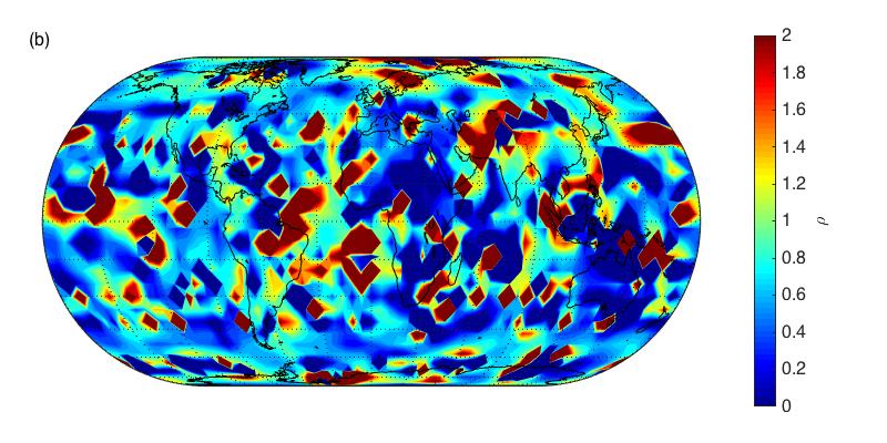
Figure 10: Non/linearity of the response in terms of (a) temperature and (b) precipitation, measured by $\rho$ given by the expression (21). Any values of $\rho$ lying outside the range of the color bar are represented by the limiting red and blue colors.

In the last column of Table 3, we show $\rho$ for the global averages $[T_{s}]$ and $[P_{y}]$ [not the average of the gridpoint-wise $\rho$’s, but having, e.g., $\Psi=[T_{s}]$ in Eq. (21)]. The steady-state values are estimated by taking the temporal mean of the ensemble means in the last 80 years. These values could be somewhat inaccurate because of the drift seen in Figs. 2(b) and 7(b) for the BR1 simulation. But considering the possible maximum values of $\rho$ for both $\Psi=[T_{s}]$ and $[P_{y}]$, a degree of nonlinearity still seems very likely. The figures indicate that the response of the global average precipitation, unlike the local values/regional averages, is not significantly more nonlinear than the response of temperature under geoengineering. These results caution us about the reliability of linear predictions of side-effects as part of an assessment exercise:

• linear predictions of regional responses are less reliable than the global response;

• some quantities can respond more nonlinearly than others.

V Summary and Outlook

As our objective (O1), we defined and solved an inverse problem for finding a solar forcing that can cancel global warming when applied in conjunction with a given greenhouse forcing. Our novel inverse problem approach is generic in two respects. First, we can allow for different choices of the scalar observable to keep under control—different either with respect to the physical quantity, or considering, for example, local variables. Second, we can prescribe an arbitrary time evolution of the chosen observable, assessing perhaps less stringent requirements than total cancellation.Helwegen et al. (2019) The inverse problem itself was derived in the framework of linear response theory. We have then further generalized the problem to the case when we want to control $N$ climatic observables by including $N$ auxiliary forcings.

Because of a degree of nonlinearity of the response characteristics of interest, the degree of approximation of the solution of the inverse problem, specifically for the cancellation of global average surface air temperature, depended on the accuracy of determining the linear susceptibilities (or Green’s functions) belonging to the different forcings. The inaccurate determination of the linear susceptibilities stems from the fact that for the estimation of the Green’s functions we used finite-magnitude external system identification forcings (see Appendix B), in which case the nonlinearity of the response is already felt, while for the cancellation, i.e., zero total response, we would need the linear susceptibilities exactly—assuming the response is linear under combined forcing. An inaccurately predicted required solar forcing leads to a nonzero residual true total response. By a simple method, however, also used by Gritsun and Lucarini Gritsun and Lucarini (2017) and independently by Liu et al.,Liu et al. (2018) here, for determining the susceptibilities, we eliminate even-order nonlinearities from the response in the system identification experiments. The price of this is having to run twice as many ensemble simulations for system identification. In the scenario of doubling CO₂ concentration, by this method we were able to achieve a fivefold reduction of the unwanted actual total response arising instead of cancellation. Furthermore, the linear prediction of spatial patterns using the improved local susceptibilities improved dramatically.

Nevertheless, the prediction is not perfect, and, pursuing our objective (O2), we indicated that the response under combined forcing should be somewhat nonlinear, and the degree of nonlinearity could be typically stronger for some quantities. In particular, we have seen evidence suggesting that in PlaSim the response of precipitation is more nonlinear than that of the surface temperature. This casts a shadow over the use of linear response theory for an efficient assessment. Perhaps there would still be value in this method, since larger-scale quantities are expected to be better predictable. Results reported by Cao et al. Cao et al. (2015) seem to indicate that in complex models this nonlinearity is not more modest. Therefore, it would be desirable in the future to work out a method of predicting the nonlinear response in geoengineering scenarios.

We note that the nonlinearity seen in the system identification experiments is not a local property of the unforced system. The nonlinearity starts to be manifested at a certain level of the response. This is the case only for the positive radiative forcing, but not for the negative one. This is why—despite the nonlocality of nonlinearity—our improved methodology in Sec. IV.1 still worked so well: the wrong susceptibility estimated from the positive forcing was averaged by the more correct susceptibility estimated from the negative forcing. That is, the error was mitigated.

Ours is the first such analysis of the linearity of regional response under geoengineering; previous studies MacMartin and Kravitz (2016); Cao et al. (2015) only compared the linear prediction and the true model response, and, as we have argued, such a comparison has to be considered inconclusive regarding the nonlinearity of the response. There is a question as to whether our findings on the predictive power of linear response theory in PlaSim carry over to state-of-the-art Earth System Models, because these do respond more weakly. The question certainly seems valid, however, since CMIP5 models also feature nonlinear regional responses under [CO₂] forcing alone.Good et al. (2015); Winton (2013) The responses of global average surface air temperature and precipitation have been reported by MacMartin and Kravitz MacMartin and Kravitz (2016) to be approximately linear in some CMIP5 models, seemingly more so than in PlaSim, but weaker forcing than [CO₂]-doubling was considered, and the linearity of regional responses was not analyzed in detail. In apparent contradiction, Cao et al. Cao et al. (2015) reported a clear and not insignificant mismatch of the linear prediction and model simulation for local responses. However, only a single state-of-the-art model was considered, the HadCM3L model, and so it was not indicated whether this is typical behavior of state-of-the-art models. Furthermore, to reiterate, regarding the novel contribution (O2) of our work, we claim that, based on these previous results reported, it was not correct to conclude that the mismatch was due to nonlinearity. As the latest result on the linearity of the local precipitation response, however, Ref. Simpson et al., , analyzing the Geoengineering Large Ensemble of the CESM1 model, states that “While a rather extreme geoengineering scenario has been considered, many, but not all, of the precipitation features scale linearly with the offset global warming.” In particular, see their Figs. 16 (c), (g), (k). Furthermore, we learn from Figs. 9 and 10 of Ref. Laakso et al., 2019 that different ESMs feature quite different patterns of local temperature and precipitation response under geoengineering.

We pointed out also that instead of stepwise system identification forcing, it is better to use a Kronecker delta forcing to achieve a better signal-to-noise ratio. As another gain from using a Kronecker delta forcing, the response would be much more modest in magnitude, and hence it would stay farther away from regimes with more significant contributions of nonlinear terms, and so the linear susceptibilities could be estimated more accurately, even by the naive method [see Appendix B and Eq. (23)].

We note that the presented method for predicting a required solar forcing is based on Green’s functions that are determined by externally forcing the system of interest. This is clearly not a method that could be put in practice in the case of the Earth system, and so we are restricted to using climate models. Therefore, this is another reason, beside the unpredictability of twenty-first century greenhouse forcing, why the method is suitable only for scenario analyses. However, it might be possible to estimate the Green’s functions without externally forcing the system, just from an observation of unforced fluctuations. The crucial question in this regard is whether the fluctuation–dissipation theorem Kubo (1966); Leith (1975) is applicable.

Appendix A Computing the response in time and frequency domains

To be able to carry out (approximate) calculations involving spectral transforms, we need to clarify the formulae and algorithms applicable to discrete-time and finite-size data. We can approximate the time-continuous forcing $f(t)$ [appearing in Eq. (4)] by a staircase-like forcing that is defined by a uniform sampling of $f(t)$, called a sample-and-hold approximation. It can be represented by a discrete sequence $f[n]=f(t=nT)$, $n=\dots,-1,0,1,\dots$, with $T$ being the uniform sampling interval, in which sequence the data points provide the levels of the “stairs.” That is, for an actual staircase-like forcing signal, $f(t=(n+\nu)T)=f[n]$ for all $\nu\in[0,1]$, where the noninteger $\nu$ can be viewed as a phase variable—the phase where the sample is taken within the interval where the forcing is constant. For such staircase-like forcings, sample values of the response with the sampling $\Psi[n]=\Psi(t=(n+\nu)T)$ of the time-continuous response at any phase $\nu\in[0,1]$ obey

$$\langle\hat{\Psi}\rangle^{(1)}[n]=\sum^{\infty}_{k=-\infty}h_{\Psi}[k]f[n-k]=h_{\Psi}[n]\ast f[n],$$ (22)

where the discrete-time (DT) impulse response or DT Green’s function $h_{\Psi}[n]$ is, clearly, the response $\langle\hat{\Psi}_{\perp}\rangle^{(1)}$ to a Kronecker delta function forcing: $f[n]=\delta[n]=1$ if $n=0$ and 0 otherwise.Hespanha (2009) Note that we make a distinction in our notation with regard to the special forcing such that we distinguish $\hat{\Psi}$ from $\Psi$; however, for simplicity, we did not subscript $\hat{\Psi}$ by $\nu$, despite its dependence on the phase. Note also that the DT impulse response function cannot be obtained by a straightforward sampling of the Green’s function; that is, in general, $h_{\Psi}[n]\neq G_{\Psi}^{(1)}[n]=G_{\Psi}^{(1)}(t=(n+\nu)T)$ with the same $\nu$ as $\Psi[n]$ (or $\hat{\Psi}[n]$) is defined with, or with any other fixed $\nu$, for all $n$. If the sampling frequency is not adequate regarding some typical time scales of the forcing, then the calculated discrete response will be also an inadequate approximation. We note further that—unlike the Dirac delta in the continuous-time case—the Kronecker delta can be realized for numerical purposes. It is equivalent to applying a step forcing and taking the difference:

$$h_{\Psi}[n]=\Delta\langle\hat{\Psi}_{\ulcorner}\rangle[n]-\Delta\langle\hat{\Psi}_{\ulcorner}\rangle[n-1].$$ (23)

This method was used by Lucarini et al. Lucarini, Ragone, and Lunkeit (2017) Such external forcings we will refer to as (system) identification forcing.

When faced with the practical situation of having finite time series, $f[l]$ and $h_{\Psi}[l]$, $l=0,\dots,L-1$, Eq. (D) of Appendix D can be used to determine the response $h_{\Psi}\ast f[l]$, $l=0,\dots,L-1$. The usefulness of this formula is due to the existence of efficient algorithms for evaluating the discrete Fourier transform, DFT; we evaluate the DFT using fft from MATLAB. To use the formula, one can pad $f[l]$ and $h_{\Psi}[l]$ by $L-1$ zeros in front (or rather $L$ zeros); we will denote these padded sequences by e.g. $\tilde{f}[l]$, $l=0,\dots,2(L-1)$. The first useful “half” ($l=0,\dots,L-2$) of the circular convolution ${\rm DFT}^{-1}\{{\rm DFT}\{\tilde{h}_{\Psi}\}{\rm DFT}\{\tilde{f}\}\}$ resulting from Eq. (D) will then match the linear convolution $h_{\Psi}\ast f[l]$, $l=0,\dots,L-1$. Unlike this calculation in the frequency domain, the calculation in the time domain using Eq. (22) is straightforward.

Appendix B Obtaining the Green’s function

First, to predict the response (to first order), we need to obtain for example the (first-order) Green’s function. As Eq. (5) suggests, it is fully determined by the autonomous system. A direct evaluation of this formula is, however, prone to failure.Lucarini, Ragone, and Lunkeit (2017) Second, we note that in practice we can study only a discrete-time version of the system. This suggests that for a direct way of determining the Green’s function, instead of Eq. (4), we have to use Eq. (22) [leading to Eq. (23)]. It also means that we cannot infer the response of the system just by observing its autonomous dynamics, but we need to force it externally in a suitable way. Third, an ensemble of experiments (appropriately initialized) is needed to obtain the expected value $\langle\hat{\Psi}\rangle$ [with the notation introduced in Appendix A, first appearing in Eq. (22)]. This was acknowledged also by MacMartin and Kravitz. MacMartin and Kravitz (2016) However, it is feasible to run only a finite number of experiments, so we obtain an approximation of $\langle\hat{\Psi}\rangle$, where the error is some correlated noise process. This correlation can be made negligible by using a suitably infrequent sampling, allowed by, say, the application of a slow forcing. We use the same data as Lucarini et al., Lucarini, Ragone, and Lunkeit (2017) which consist of some ensembles of 200 members, and we have produced new data belonging to new forcing scenarios, as described in Sec. II, that consist of ensembles of 20 members.

As already spelled out in Appendix A, two identification forcing types are particularly suitable to determine the Green’s function: one is a step forcing, and the other is the Kronecker delta. When a random statistical error is present due to the finite ensemble size, represented say by a Gaussian random variable $\xi$, it is actually better to use a Kronecker delta forcing for the following reason. Using the step forcing instead, one needs to take the difference of consecutive values—what is sometimes called “differencing”—of the response sequence (23). This way, at any time, the variance of the error is that of the difference of two random variables, $\xi_{1}$ and $\xi_{2}$, both distributed identically to the original random variable $\xi$. For Gaussian variables, it is straightforward to show that ${\rm Var}[\xi_{1}-\xi_{2}]=2{\rm Var}[\xi]$. Note that we assume that $\xi$ is the same random variable to a good approximation under the delta and step forcings. Despite the advantage of the Kronecker delta forcing, we apply a step forcing also in our new experiments, so that we are able to make use of data produced for the study by Lucarini et al. Lucarini, Ragone, and Lunkeit (2017) in a consistent manner. Examples of the response to step forcings are displayed in Fig. 11. The similarity of the responses to greenhouse and solar forcings here, and so the Green’s functions, is consistent with the findings of others Merlis et al. (2014); Caldeira and Myhrvold (2013); MacMynowski, Shin, and Caldeira (2011) and the design of the G2 GeoMIP experiment.Kravitz et al. (2011)

It is important to appreciate the following trade-off. For a better signal-to-noise ratio (SNR), one can apply a more powerful identification forcing. However, in the presence of nonlinearities, the more powerful the forcing signal, the larger is the error in estimating the Green’s function belonging to the base state $\langle\Psi\rangle_{0}$ (even without noise). MacMartin and Kravitz MacMartin and Kravitz (2016) applied a [CO₂]-quadrupling (and this is a standard forcing level for geoengineering studies Ferraro, Highwood, and Charlton-Perez (2014); Kravitz et al. (2011)); however, they did not determine the solar forcing for cancellation via Green’s functions (Appendix C), and they checked the linearity of the response only up to a forcing level lower than [CO₂]-doubling. Their motivation for applying the high forcing level seems to have been only to be able to determine the Green’s function with a better SNR given that no ensemble data are available from the GeoMIP experiments.

We make here two more comments about the issue with noise. First, instead of instantaneous samples of the observable $\Psi$ and the corresponding Green’s function, we will consider, like Lucarini et al.,Lucarini, Ragone, and Lunkeit (2017) annual averages, $\bar{\Psi}[n]=\int_{0}^{1}\mathrm{d}\nu\Psi((n+\nu)T)$. This is sensible given the slow rate of change that the applied forcing represents, and it also greatly reduces the noise level. In this regard, we point out that annual averages too obey Eq. (22) exactly if the forcing is constant over a year, because the order of summations can be interchanged, whereby a well-defined DT Green’s function belonging to the annual average emerges. We will use only annually constant staircase-like forcings in our experiments (Sec. II), so that it will be clear that a linear prediction of the response has an error not because Eq. (22) does not apply exactly, but because of the missing higher-order perturbative terms appearing in the expression (2). Second, the said enhancement of noise by differencing in Eq. (23) cannot be overcome by working in the frequency domain. The Green’s function, via the frequency domain and applying Eq. (28) of Appendix D, is expressed as $h_{\Psi}={\rm DTFT}^{-1}\{{\rm DTFT}\{\Delta\langle\hat{\Psi}_{\ulcorner}\rangle\}/{\rm DTFT}\{f_{\ulcorner}\}\}$, where $1/{\rm DTFT}\{f_{\ulcorner}\}=1-e^{-i\omega}$. The latter is the very factor arising in the DTFT of a differenced sequence. As far as we are aware, the only way to avoid the differencing and thereby reduce the noise is by using a Kronecker delta identification forcing as argued above.

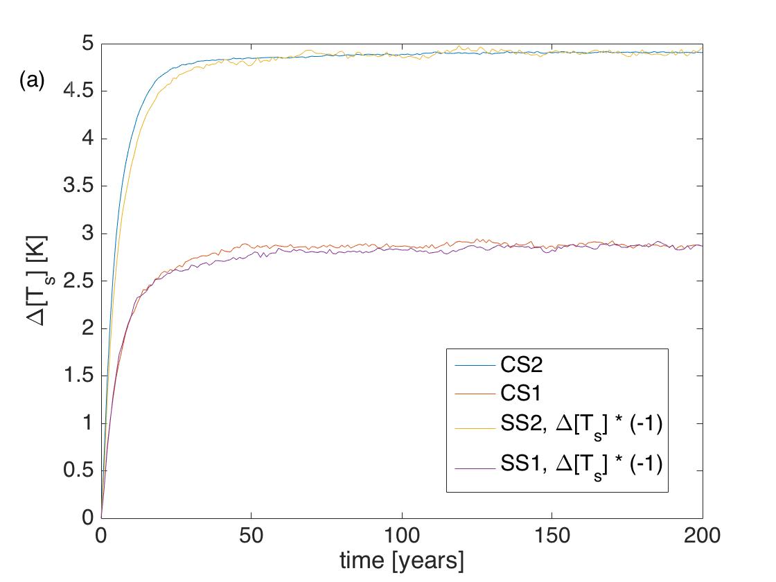
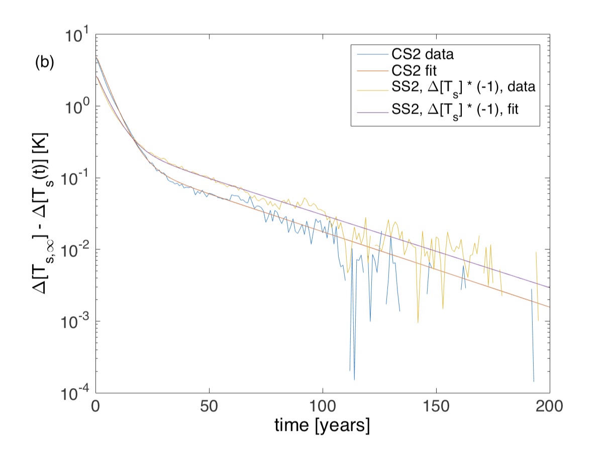
Figure 11: Simulated response to step forcings. The chosen observable is the global average surface air temperature $[T_{s}]$. The identification forcing scenarios are those of CS2, CS1, SS2, and SS1 from Table 1. After a subtraction of the limit value and displaying the response on linear–log scales in (b), it is revealed that the high-dimensional system behaves very much like a noise-driven linear two-box model, also called a vector autoregressive (VAR) model, in view of the considered global scale variable, as also recognized by MacMynowski (MacMartin) et al. MacMynowski, Shin, and Caldeira (2011) and Caldeira and Myhrvold.Caldeira and Myhrvold (2013) The two time scales of the VAR models fitted to the CS2 and SS2 data are about 5 and 40 years. The second time scale is in disagreement with MacMynowski (MacMartin) et al.,MacMynowski, Shin, and Caldeira (2011) and it is not clear whether a more complex model is more reliable in this respect. Note: the angle brackets denoting ensemble average are dropped from diagram annotations throughout this paper.

We also note that the application of a stepwise identification forcing implies a specific frequency dependence of the variance of the estimator of the susceptibility. See Ref. Kravitz et al., 2017b for other system identification techniques that imply different such frequency dependences.

Appendix C The inverse problem

When different forcings act at the same time, their first-order contributions to the response—as discussed in Sec. I.1—can be superimposed. Hence, when we desire a certain total response $\Delta\langle\Psi_{\varSigma}\rangle(t)$ to a combined forcing when all forcings are given but one, there is a unique form of that one required forcing to fulfill our desire. In terms of the geoengineering problem of interest (Sec. I.2), the required solar forcing $f_{s}$ to achieve a total response $\Delta\langle\Psi_{\varSigma}\rangle$ given a greenhouse forcing $f_{g}$ can be expressed, to a first-order approximation, in the frequency domain as stated in Eq. (10). With the most obvious choice of cancellation, $\Delta\langle\Psi_{\varSigma}\rangle=0$, Eq. (10) simplifies to

$$f_{s}(\omega)\approx-\frac{\chi_{\Psi,{g}}(\omega)}{\chi_{\Psi,s}(\omega)}f_{g}(\omega).$$ (24)

However, in practice, when finite time series are available, the simplification is not so trivial. As described at the end of Appendix A, in place of the three FTs in Eq. (10), we have to evaluate DFT$\{\tilde{f}_{g}\}$, DFT$\{\tilde{h}_{\Psi,s}\}$ and DFT$\{\tilde{h}_{\Psi,{g}}\}$. Furthermore, the DFT in place of $\Delta\langle\Psi_{\varSigma}\rangle(\omega)$ is that of a sequence $\Delta\langle\check{\Psi}_{\varSigma}\rangle[l]$, only the first useful “half” ($l=0,\dots,L-2$) of which is zero, as dictated by our requirements, but its second half ($l=L-1,\dots,2(L-1)$) has nonzero values in general. That is, what we have is

$$\tilde{f}_{s}={\rm DFT}^{-1}\{( {\rm DFT}\{\Delta\langle\check{\Psi}_{\varSigma}\rangle\}$$

$$-{\rm DFT}\{\tilde{h}_{\Psi,{g}}\}{\rm DFT}\{\tilde{f}_{{g}}\})/{\rm DFT}\{\tilde{h}_{\Psi,s}\}\},$$ (25)

It can be shown that the said nonzero values characterize the total response to combined step forcings (to do with the “gap” mentioned in the caption of Fig. 12), but also depend to a certain extent on the particular finite $f_{g}[l]$ presented. The reason for this is that the Green’s function is given only up to a finite time, which becomes clear upon inspection of the workings of the convolution of finite time series. Simply by rearranging Eq. (C), the said nonzero values are given by

$$\Delta\langle\check{\Psi}_{\varSigma}\rangle={\rm DFT}^{-1}\{ {\rm DFT}\{\tilde{h}_{\Psi,{g}}\}{\rm DFT}\{\tilde{f}_{{g}}\}$$

$$+{\rm DFT}\{\tilde{h}_{\Psi,s}\}{\rm DFT}\{\tilde{f}_{s}\}\},$$ (26)

where, however, $\tilde{f}_{s}$ is not known, being the sought-for object. The idea is that we can look for $\tilde{f}_{s}$ by an iterative procedure, which is initialized, say, by $\tilde{f}_{s}=\tilde{f}_{g}$. Note that if $h_{\Psi,{g}}$ and $h_{\Psi,s}$ are not dissimilar, then nor are $f_{g}$ and $f_{s}$; that is, the initial value is not far from the solution, which gives hope that it is within the basin of attraction of the solution. In each iterate, we do the following:

1. Evaluate Eq. (C) using the current estimate of $\tilde{f}_{s}$, but instead of simply substituting this value, first we replace any nonzeros in its first half by zeros.

2. In the resulting $\Delta\langle\check{\Psi}_{\varSigma}\rangle[l]$, we replace any nonzeros in its first half by zeros in order to have it in the right form.

3. We then get a new estimate for $\tilde{f}_{s}$ using Eq. (C).

Ideally, the first half of the $\tilde{f}_{s}$ estimates in stage 3 converge to zero, and the second half to some nontrivial form that is the solution. In our experience (results not shown), this is the case for systems with fairly simple and smoothly varying Green’s functions. However, when the same Green’s functions are corrupted by noise (which arises in practice from the finiteness of the ensemble size; see Appendix B), our experience is that the procedure does not necessarily converge, but iterates of $\tilde{f}_{s}$ can develop increasingly large oscillatory features. It is possible to achieve convergence for some smaller but nonzero noise level. However, even then, the limit function retains small oscillatory features over the full length of $\tilde{f}_{s}$.

We emphasize that the iterative procedure was needed because we could not predict the second non-useful half of $\Delta\langle\check{\Psi}_{\varSigma}\rangle[l]$, since we do not have the Green’s functions in full but only with a cutoff in time. This means that by running longer and longer ensemble simulations, by which we can determine the Green’s functions further and further in time, the solution can be approximated by a noniterative procedure better and better. This is a numerically more expensive solution.

As an alternative, working in the time domain, the inverse problem leads to the performance of a deconvolution:

$$f_{s}=(\Delta\langle\check{\Psi}_{\varSigma}\rangle-h_{\Psi,{g}}\ast f_{g})\ast^{-1}h_{\Psi,s}.$$ (27)

Note that we have written $\Delta\langle\check{\Psi}_{\varSigma}\rangle[l]$ in the above, which should correspond exactly to the appropriately defined circular convolution in Eq. (C) for $l=0,\dots,2(L-1)$. It is straightforward to show that in the time domain too, $f_{s}[l]$, $l=0,\dots,L-1$, is obtained iteratively in three stages in a similar manner as outlined above in the frequency domain (except that in stage 1, there is no need to replace any values by zeros, only in stage 2). One can use deconv in MATLAB to perform the deconvolution. We find in simple examples studied (results not shown) that without noise the procedure in the time domain leads to the very same solution as the procedure in the frequency domain. However, this is not the case with additive noise, which means that the deconvolution/inverse problem is ill-posed in this case. Nevertheless, the weaker the noise, the closer the outcome is to the true solution, either in the time or the frequency domain. We find that in the time domain, the procedure always converges to some solution; however, with increasing noise strength, this solution features oscillations of increasing amplitude as time advances. Nevertheless, for a certain noise strength when the frequency-domain procedure also converges, we find that the solution in the time domain is smoother and so closer to the true solution earlier in time. This is also what we find considering the PlaSim data, as shown in Fig. 12. We conclude, therefore, that it is preferable to work in the time domain using Eq. (27) to produce numerical results. Nevertheless, we will carry out our calculations in the frequency domain, using for example the forcing signals shown in Fig. 12(a), in order to make the point that even a rough forcing signal convolved with a rough Green’s function produces a not so rough response, as we see in Sec. III.1.1.

We emphasize that, in our case, multiple iterations are not needed, because $h_{[T_{s}],{g}}$ and $h_{[T_{s}],s}$ are very similar, as indicated by Fig. 11. The straightforward application of Eq. (C) is sufficient, substituting an all-zero sequence for $\Delta\langle\check{\Psi}_{\varSigma}\rangle$. Ours is obviously a special case, however, and the generic iterative procedure might be needed for other geoengineering scenarios of practical relevance.

We note that an anonymous referee of a previous submission of this paper had suggested that, in the time domain, a simpler alternative way of obtaining the solution by a time-marching procedure should exist (not relying on deconvolution). Indeed, one can break down the convolution sum (22) as $\langle\hat{\Psi}\rangle^{(1)}[n]=\sum^{n}_{k=2}h_{\Psi,s}[k]f_{s}[n-k]+h_{\Psi,s}[1]f_{s}[n-1]$, which can be expressed for $f_{s}[n-1]$ and consider that $\langle\hat{\Psi}\rangle^{(1)}[n]=\sum^{n}_{k=1}h_{\Psi,g}[k]f_{g}[n-k]$ is given for all $n$. Suppose $f_{g}[0]=0$; then the procedure for finding $f_{s}[n-1>0]$ can be initialized by $f_{s}[0]=0$ for $n=1$. We have checked (results not shown) that it gives exactly the same result as our iterative procedure, reproducing the time series pattern due to a particular noise realization in a simple example system.

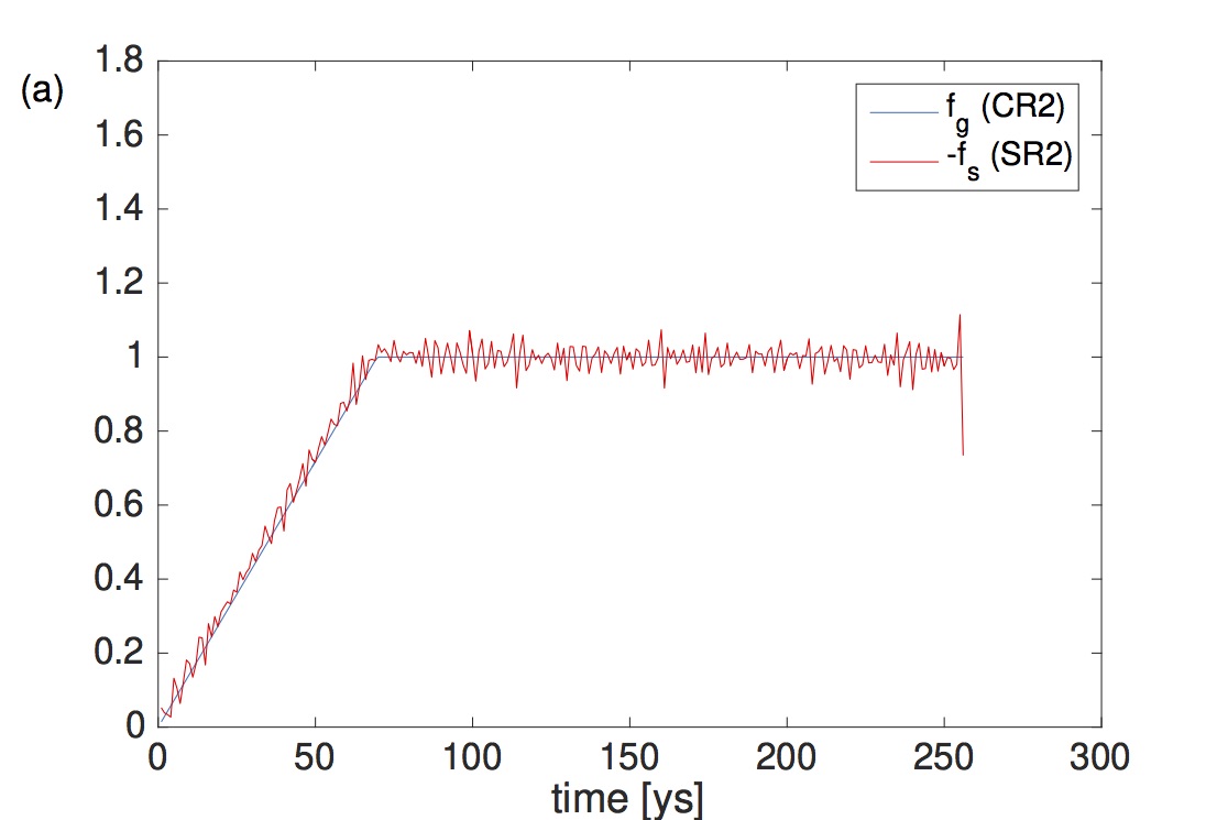
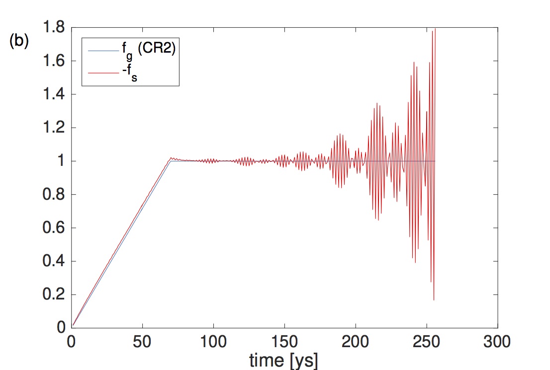
Figure 12: Imposed $[{\rm CO}_{2}]$ or greenhouse forcing and required solar forcing that cancels out global average surface air temperature change. Values of the time series are normalized for the purpose of display, so that they have a unit plateau level. The required solar forcing is determined in both the frequency domain (a) and the time domain (b). We indicate in the keys the data sets from Table 1 to which the forcings belong. We note that in either case, we neglected the iteration, skipping stages 1 and 2 and setting $\Delta\langle\check{\Psi}_{\varSigma}\rangle[l]=\Delta\langle\check{[T_{s}]}_{\varSigma}\rangle[l]=0$ for all $l$ straightaway in stage 3, the validity of which is suggested by the very similar Green’s functions $h_{[T_{s}],{g}}$ and $h_{[T_{s}],s}$, as indicated by Fig. 11. Correspondingly, the required $f_{s}$ is very similar to the given $f_{g}$. A small gap between the red and blue ramps that can be resolved only with a smooth estimate [i.e., in (b) but not in (a)] informs us that the system responds slightly faster to the greenhouse forcing. This characteristic was already suggested by Fig. 11(b) and the exact results of the parameter estimation by fitting. Results presented in Sec. IV.2 suggest that it is likely to do with nonlinearity, which makes the responses to negative and positive anomalies “asymmetric,” resulting also in different spatial patterns, while the time scales associated with different locales are quite varied (results not shown).

Appendix D The circular convolution theorem and its application

Taking the discrete-time Fourier transform (DTFT) of Eq. (22), we have, via the convolution theorem for discrete sequences Katznelson (1976), a formally analogous version of Eq. (6), with the individual Fourier transforms approximated by Fourier series:

$$\langle\hat{\Psi}\rangle^{(1)}_{2\pi}(\omega)=\hat{\chi}_{\Psi,2\pi}(\omega)f_{2\pi}(\omega),$$ (28)

where, for example, $f_{2\pi}(\omega)={\rm DTFT}\{Tf[n]\}=\sum_{n=-\infty}^{\infty}Tf[n]e^{-i\omega n}$ and $f[n]={\rm DTFT}^{-1}\{T^{-1}f_{2\pi}(\omega)\}=\frac{1}{2\pi T}\int_{-\pi}^{\pi}d\omega f_{2\pi}(\omega)e^{i\omega n}$ with a normalized nondimensional angular frequency $\omega$. Featuring instead the dimensional frequency $f$ measured in hertz (1  Hz = 1 s^-1), the forward and inverse transform pairs are symmetrical: $f_{1/T}(f)=f_{2\pi}(2\pi fT)=\sum_{n=-\infty}^{\infty}Tf[n]e^{-i2\pi fTn}$ and $f[n]=T\int_{1/T}dff_{1/T}(f)e^{i2\pi fTn}$. The DTFT, a continuous function of the frequency $f$, is often sampled at $f=k/(NT)$, $k=0,\dots,N-1$:

$$f_{1/T}(k/(NT)) =T\sum_{n=-\infty}^{\infty}f[n]e^{-i2\pi kn/N}$$

$$=T\sum_{n=n_{0}}^{n_{0}+N}f_{N}[n]e^{-i2\pi kn/N}$$

$$=T\times{\rm DFT}\{f_{N}[n=n_{0},\dots,n_{0}+N]\},$$ (29)

for any $n_{0}$, which yields the discrete Fourier transform (DFT) of the finite sequence $f_{N}[n]$, $n=n_{0},\dots,n_{0}+N$, where the full infinite sequence $f_{N}[n]$, $n\in\mathbb{R}$, turns out to be $N$-periodic, since it has to be, for the equivalence of the two sums in Eq. (D), in the so-called periodic summation form

$$f_{N}[n]=\sum_{m=-\infty}^{\infty}f[n-mN].$$ (30)

Therefore, when $f[n]$ is actually $N$-periodic, its DTFT is nonzero only at $f=k/(NT)$, $k\in\mathbb{R}$, and also periodic, such that the DFT of a single cycle of $f[n]$ is able to represent its DTFT. For such periodic sequences, to be denoted distinctively using a subscript as $f_{N}[n]$, it can be proved Katznelson (1976) that

$$y\ast f_{N} ={\rm DTFT}^{-1}\{{\rm DTFT}\{y\}{\rm DTFT}\{f_{N}\}\}$$

$$={\rm DFT}^{-1}\{{\rm DFT}\{y_{N}\}{\rm DFT}\{f_{N}\}\},$$ (31)

for any nonperiodic sequence $y[n]$. Note that $y\ast f_{N}$ is referred to as the circular convolution of the sequences $y[n]$ and $f[n]$. When the sequences $y[n]$ and $f[n]$ are of finite length, $n=0,\dots,N-1$ with any $N\geq 1$, so that, for example, $f_{N}[n]=f[{\rm mod}(n,N)]$, their circular convolution can be shown to be Katznelson (1976) (see also https://uk.mathworks.com/help/signal/ug/linear-and-circular-convolution.html)

$$(y\ast f_{N})[n=0,\dots,N-1] =\sum_{k=0}^{N-1}y[k]f_{N}[n-k]$$

$$={\rm DFT}^{-1}\{{\rm DFT}\{y\}{\rm DFT}\{f\}\}.$$ (32)

This equality is called the circular convolution theorem. It follows that when $y[n]=0$ and $f[n]=0$ for $n=0,\dots,N_{f}-1$ and $N_{y}-1$, respectively, then $(y\ast f_{N})[{\rm mod}(n-1,N)]=(y\ast f)[n]$ for $n=N,\dots,N+{\rm min}(N_{f}+N_{y},N-1)$. Furthermore, $(y\ast f)[n]$, $n=1+N_{f}+N_{y},\dots,N+1+N_{y}$, is the segment that represents the part of the linear convolution that can be considered useful in the sense that it coincides with the occurrence of the finite values of $f$ in a finite time interval of length $N-N_{f}$. Therefore, the circular convolution $(y\ast f_{N})[n]$ captures the useful part of the linear convolution over $n=\max(1+N_{f}+N_{y},N),\dots,N+\min(1+N_{y},N_{f}+N_{y},N-1)$.

Therefore, when faced with the practical situation of having finite time series, $f[l]$ and $h_{\Psi}[l]$, $l=0,\dots,L-1$, Eq. (D) can be used to determine the response $h_{\Psi}\ast f[l]$, $l=0,\dots,L-1$ (whose usefulness comes from an efficient algorithm for evaluating the DFT, called the fast Fourier transform algorithm, FFT). In particular, if the two sequences are to be padded in front by a number $N_{f}=N_{h}=N_{0}$ of zeros equally (so that the circular convolution (D) is well defined), then the reconstructed length of the linear convolution $h_{\Psi}\ast f$ (the response of a causal system coinciding with the forcing) is $1+N_{0}-\max(N_{0}-L+1,0)$. This is a linear function of $N_{0}$ saturating at $N_{0}=L-1$ reaching the full length $L$. Therefore, for simplicity one can pad by $N_{0}=L-1$ zeros,Note (5) and we will denote these padded sequences by, for example, $\tilde{f}[l]$, $l=0,\dots,2(L-1)$. Note that padding with fewer or no zeros results in a circular convolution that better approximates either the useful or the not useful part of the linear convolution, which approximation is better the more zeros are used. In the extreme case of no padding, very little of the useful part can be approximated well. The key to the applicability of Eq. (D) is that it does not matter how the forcing $f[n]$—and with it the response $\langle\hat{\Psi}\rangle[n]$—continue after our experiment, and so they can be thought of as periodic.

Appendix E Zonal average surface temperature

For the diagnostics of any residual total response, a good starting point is to look at the zonally averaged fields of the surface air temperature. As a reminder, any observable other than the one for which a desired evolution has been enforced (the global average surface air temperature in our case; see Sec. III.1.1) can evolve in an uncontrolled fashion. This is something that is not intended and should be checked. First, we show results with the $\sqrt{2}$-fold $[{\rm CO}_{2}]$ increase (CR1, BR1). Following Lucarini et al. Lucarini, Ragone, and Lunkeit (2017) (where only the case of $[{\rm CO}_{2}]$-doubling was treated), treating zonal means in a similar fashion to global means informs us that the response to either greenhouse or solar forcing is strongest at high-latitude/polar regions; see Figs. 13(a) and 13(c). This is where the response is most nonlinear, as indicated by Figs. 13(b) and 13(d), showing the difference between reference and prediction. This nonlinearity should be due to albedo saturation and/or nonlinear characteristics of radiation physics, as discussed by others.Winton (2013); Good et al. (2015); Lucarini, Ragone, and Lunkeit (2017); Liu et al. We note that in Figs. 13(b) and 13(d), nonzero values under the stationary climate (after a transient) represent finite-ensemble-size statistical errors only. As a consequence of the said nonlinearities, in the high-latitude regions, linear response theory performs very poorly in predicting the total response to combined forcing, as it does also in the regime of stationary climate; compare Figs. 14(a) and 14(b) showing the prediction and reference, respectively.

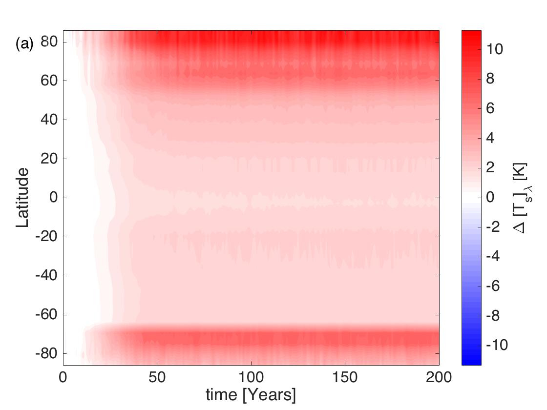
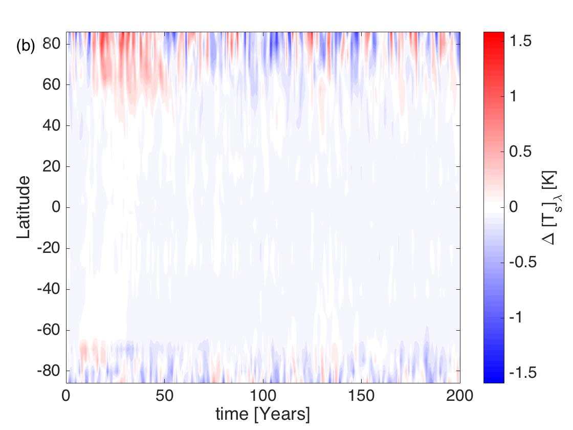
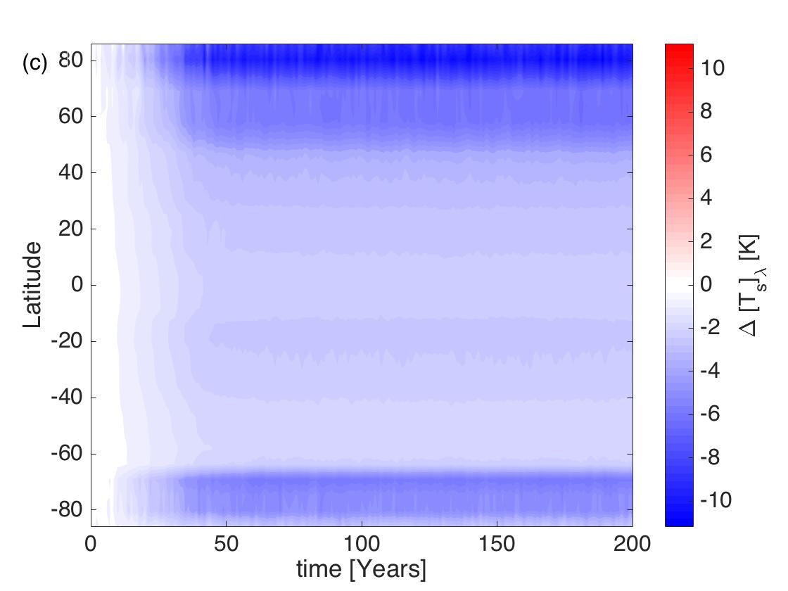
Figure 13: Response of the zonally averaged surface air temperature to ramp forcings. The first column shows the true responses in the model and the second the errors in the linear predictions. The first and second rows belong to the CR1 and SR1 forcing scenarios, respectively. Similar diagrams as in the first row but for CR2 are shown in Fig. 6 of Ref. Lucarini, Ragone, and Lunkeit, 2017.

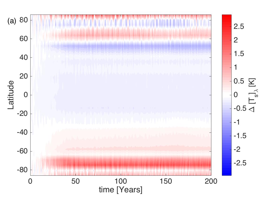
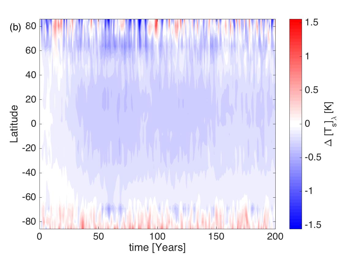
Figure 14: Predicted (a) and true (b) total responses of the zonally averaged surface air temperature to combined ramp forcings (BR1).

In addition to such a visual comparison, it is customary to quantify the discrepancy by measuring the error of the prediction relative to the true value. However, the true value can be zero at certain latitudes, and this naive relative error measure then lacks an obvious meaning. In these situations, it is customary Tornqvist, Vartia, and Vartia (1985) to analyze the following relative error:

$$e_{1}=\frac{|\Delta\langle\Psi\rangle_{BRX}-\langle\Psi\rangle^{(1)}_{BRX}|}{|\Delta\langle\Psi\rangle_{BRX}|+|\langle\Psi\rangle^{(1)}_{BRX}|}.$$ (33)

This takes values in the interval [0,1] for all values of $\Delta\langle\Psi\rangle_{BRX}$ and $\langle\Psi\rangle^{(1)}_{BRX}$; and a larger value should be considered worse. Clearly, $e_{1}(\mu)$ as a function of latitude would facilitate the comparison of the predictive skill of linear response theory at different latitudes. We note that in Eq. (33), $\langle\Psi\rangle^{(1)}_{BRX}$ is meant to be an estimator of the actual quantity, and this estimator is biased, but to keep things simple, we do not introduce a separate symbol for the estimator. Another possibility in our situation is that we measure the error of prediction of the response to combined forcing relative to the response to one of the forcings:

$$e_{2}=\frac{|\Delta\langle\Psi\rangle_{BRX}-\langle\Psi\rangle^{(1)}_{BRX}|}{\Delta\langle\Psi\rangle_{CRX}}.$$ (34)

We evaluate $e_{1}$ and $e_{2}$ only with respect to the stationary climate, in which case the estimation is very accurate since we can take an average also with respect to time. Figure 15(a) shows the result in the case of the weaker forcing (CR1, BR1). Both $e_{1}$ and $e_{2}$ indicate with good agreement that the prediction is poorest at some high-latitude regions.

With $[{\rm CO}_{2}]$-doubling (CR2, BR2), as shown by the results in Fig. 15(b), the performance has different characteristics in comparison with the case of weak forcing. Both $e_{1}$ and $e_{2}$ are highest at both equatorial and some high-latitude regions, and somewhat less at polar and some Southern Hemisphere midlatitude regions.

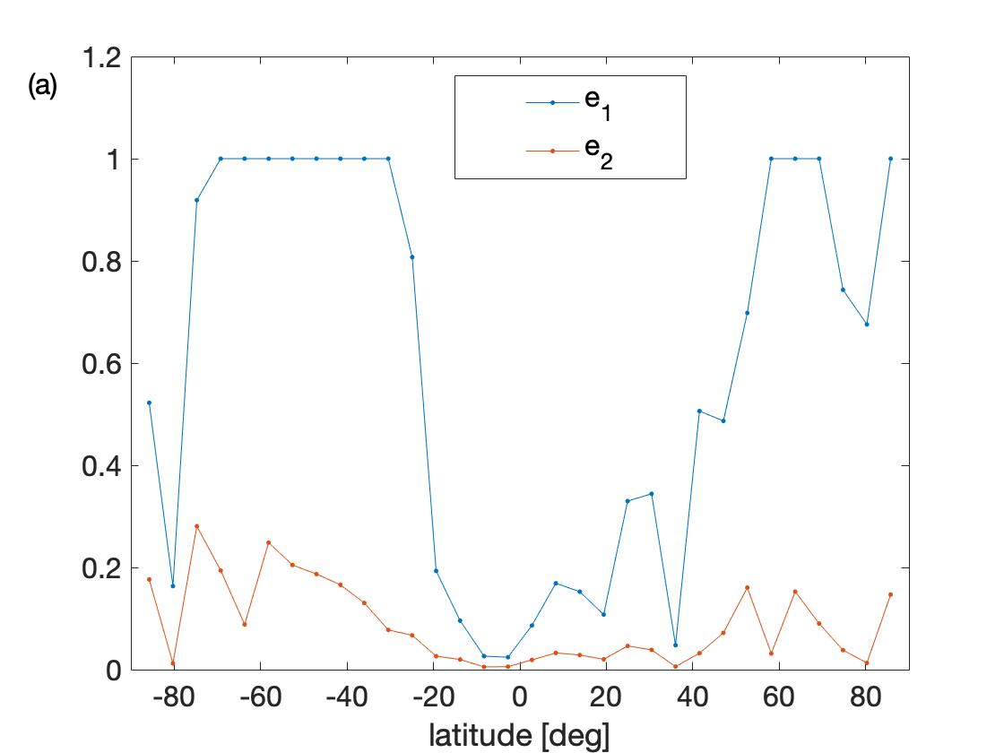
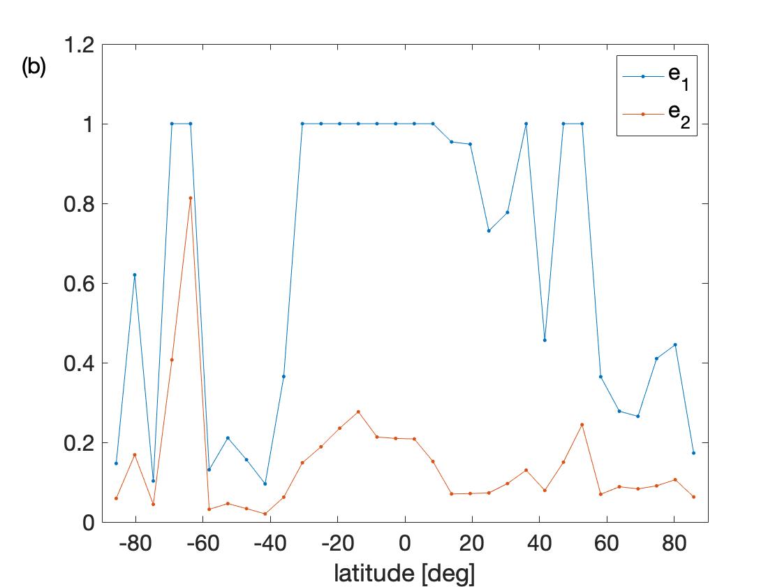
Figure 15: Relative errors $e_{1}$ and $e_{2}$ defined respectively by Eqs. (33) and (34) for the predicted total responses of the zonally averaged surface air temperature to combined ramp forcings. (a) is a companion diagram to those in Figs. 13 and 14 belonging to the weak-forcing scenarios (CR1, BR1), whereas (b) shows the same for the stronger-forcing scenarios (CR2, BR2). Discrete data points are connected by lines to aid reading the diagrams.

References

- Allen et al. (2014) M. R. Allen, V. R. Barros, J. Broome, W. Cramer, R. Christ, J. A. Church, L. Clarke, Q. Dahe, P. Dasgupta, N. K. Dubash, O. Edenhofer, I. Elgizouli, C. B. Field, P. Forster, P. Friedlingstein, J. Fuglestvedt, L. Gomez-Echeverri, S. Hallegatte, G. Hegerl, M. Howden, K. Jiang, B. Jimenez Cisneros, V. Kattsov, H. Lee, K. J. Mach, J. Marotzke, M. D. Mastrandrea, L. Meyer, J. Minx, Y. Mulugetta, K. O’Brien, M. Oppenheimer, R. K. Pachauri, J. J. Pereira, R. Pichs-Madruga, G.-K. Plattner, H.-O. Pörtner, S. B. Power, B. Preston, N. H. Ravindranath, A. Reisinger, K. Riahi, M. Rusticucci, R. Scholes, K. Seyboth, Y. Sokona, R. Stavins, T. F. Stocker, P. Tschakert, D. van Vuuren, J.-P. van Ypersele, G. Blanco, M. Eby, J. Edmonds, M. Fleurbaey, R. Gerlagh, S. Kartha, H. Kunreuther, J. Rogelj, M. Schaeffer, J. Sedláček, R. Sims, D. Ürge Vorsatz, D. Victor, and G. Yohe, IPCC Fifth Assessment Synthesis Report–Climate Change 2014 Synthesis Report, edited by P. Aldunce, T. Downing, S. Joussaume, Z. Kundzewicz, J. Palutikof, J. Skea, K. Tanaka, F. Tangang, C. Wenying, and Z. Xiao-Ye (Intergovernmental Panel on Climate Change (IPCC), 2014) p. 116.
- National Research Council (2015a) National Research Council, Climate Intervention: Carbon Dioxide Removal and Reliable Sequestration (The National Academies Press, Washington, DC, 2015).
- National Research Council (2015b) National Research Council, Climate Intervention: Reflecting Sunlight to Cool Earth (The National Academies Press, Washington, DC, 2015).
- Lenton and Vaughan (2013) T. Lenton and N. Vaughan, Geoengineering Responses to Climate Change (Springer, 2013).
- Ferraro, Highwood, and Charlton-Perez (2014) A. J. Ferraro, E. J. Highwood, and A. J. Charlton-Perez, “Weakened tropical circulation and reduced precipitation in response to geoengineering,” Environmental Research Letters 9, 014001 (2014).
- Kravitz et al. (2011) B. Kravitz, A. Robock, O. Boucher, H. Schmidt, K. E. Taylor, G. Stenchikov, and M. Schulz, “The Geoengineering Model Intercomparison Project (GeoMIP),” Atmospheric Science Letters 12, 162–167 (2011).
- Kravitz (2018) B. Kravitz, “Designer climates?” (2018).
- Helwegen et al. (2019) K. G. Helwegen, C. E. Wieners, J. E. Frank, and H. A. Dijkstra, “Complementing CO2 emission reduction by solar radiation management might strongly enhance future welfare,” Earth System Dynamics 10, 453–472 (2019).
- Stilgoe (2019) J. Stilgoe, “Shared space and slow science in geoengineering research,” in International Handbook on Responsible Innovation, edited by R. von Schomberg and J. Hankins (Edward Elgar Publishing, 2019).
- Collomb (2019) J.-D. Collomb, “US conservative and libertarian experts and solar geoengineering: An assessment,” European Journal of American Studies 14 (2019), 10.4000/ejas.14717.
- Kubo (1966) R. Kubo, “The fluctuation–dissipation theorem,” Reports on Progress in Physics 29, 255 (1966).
- Ruelle (2009) D. Ruelle, “A review of linear response theory for general differentiable dynamical systems,” Nonlinearity 22, 855 (2009).
- Sell (1967a) G. R. Sell, “Nonautonomous differential equations and topological dynamics. I. The basic theory,” Transactions of the American Mathematical Society 127, 241–262 (1967a).
- Sell (1967b) G. R. Sell, “Nonautonomous differential equations and topological dynamics. II. Limiting equations,” Transactions of the American Mathematical Society 127, 263–283 (1967b).
- Romeiras, Grebogi, and Ott (1990) F. J. Romeiras, C. Grebogi, and E. Ott, “Multifractal properties of snapshot attractors of random maps,” Physical Review A 41, 784–799 (1990).
- Crauel and Flandoli (1994) H. Crauel and F. Flandoli, “Attractors for random dynamical systems,” Probability Theory and Related Fields 100, 365–393 (1994).
- Crauel, Debussche, and Flandoli (1997) H. Crauel, A. Debussche, and F. Flandoli, “Random attractors,” Journal of Dynamics and Differential Equations 9, 307–341 (1997).
- Arnold (1998) L. Arnold, Random Dynamical Systems (Springer, 1998).
- Kloeden and Rasmussen (2011) P. E. Kloeden and M. Rasmussen, Nonautonomous Dynamical Systems, Mathematical Surveys and Monographs, Vol. 176 (AMS, 2011).
- Carvalho, Langa, and Robinson (2013) A. Carvalho, J. A. Langa, and J. Robinson, Attractors for Infinite-Dimensional Non-Autonomous Dynamical Systems (Springer, 2013).
- Leith (1975) C. E. Leith, “Climate response and fluctuation dissipation,” Journal of the Atmospheric Sciences 32, 2022–2026 (1975).
- Bell (1980) T. L. Bell, “Climate sensitivity from fluctuation dissipation: Some simple model tests,” Journal of the Atmospheric Sciences 37, 1700–1707 (1980).
- Nicolis, Boon, and Nicolis (1985) C. Nicolis, J. P. Boon, and G. Nicolis, “Fluctuation–dissipation theorem and intrinsic stochasticity of climate,” Il Nuovo Cimento C 8, 223–242 (1985).
- Cionni, Visconti, and Sassi (2004) I. Cionni, G. Visconti, and F. Sassi, “Fluctuation dissipation theorem in a general circulation model,” Geophysical Research Letters 31 (2004), 10.1029/2004GL019739, l09206.
- Gritsun and Branstator (2007) A. Gritsun and G. Branstator, “Climate response using a three-dimensional operator based on the fluctuation–dissipation theorem,” Journal of the Atmospheric Sciences 64, 2558–2575 (2007).
- Kirk-Davidoff (2009) D. B. Kirk-Davidoff, “On the diagnosis of climate sensitivity using observations of fluctuations,” Atmospheric Chemistry and Physics 9, 813–822 (2009).
- Majda, Gershgorin, and Yuan (2010) A. J. Majda, B. Gershgorin, and Y. Yuan, “Low-frequency climate response and fluctuation–dissipation theorems: Theory and practice,” Journal of the Atmospheric Sciences 67, 1186–1201 (2010).
- Cooper, Esler, and Haynes (2013) F. C. Cooper, J. G. Esler, and P. H. Haynes, “Estimation of the local response to a forcing in a high dimensional system using the fluctuation–dissipation theorem,” Nonlinear Processes in Geophysics 20, 239–248 (2013).
- Lucarini and Sarno (2011) V. Lucarini and S. Sarno, “A statistical mechanical approach for the computation of the climatic response to general forcings,” Nonlinear Processes in Geophysics 18, 7–28 (2011).
- Good, Gregory, and Lowe (2011) P. Good, J. M. Gregory, and J. A. Lowe, “A step-response simple climate model to reconstruct and interpret AOGCM projections,” Geophysical Research Letters 38 (2011), 10.1029/2010GL045208.
- Ragone, Lucarini, and Lunkeit (2016) F. Ragone, V. Lucarini, and F. Lunkeit, “A new framework for climate sensitivity and prediction: A modelling perspective,” Climate Dynamics 46, 1459–1471 (2016).
- Lucarini, Ragone, and Lunkeit (2017) V. Lucarini, F. Ragone, and F. Lunkeit, “Predicting climate change using response theory: Global averages and spatial patterns,” Journal of Statistical Physics 166, 1036–1064 (2017).
- Herein et al. (2015) M. Herein, J. Márfy, G. Drótos, and T. Tél, “Probabilistic concepts in intermediate-complexity climate models: A snapshot attractor picture,” Journal of Climate 29, 259–272 (2015).
- Herein et al. (2017) M. Herein, G. Drótos, T. Haszpra, J. Márfy, and T. Tél, “The theory of parallel climate realizations as a new framework for teleconnection analysis,” Scientific Reports 7, 44529 (2017), article.
- Bódai and Tél (2012) T. Bódai and T. Tél, “Annual variability in a conceptual climate model: Snapshot attractors, hysteresis in extreme events, and climate sensitivity,” Chaos: An Interdisciplinary Journal of Nonlinear Science 22, 023110 (2012).
- Drótos, Bódai, and Tél (2015) G. Drótos, T. Bódai, and T. Tél, “Probabilistic concepts in a changing climate: A snapshot attractor picture,” Journal of Climate 28, 3275–3288 (2015).
- Drótos, Bódai, and Tél (2016) G. Drótos, T. Bódai, and T. Tél, “Quantifying nonergodicity in nonautonomous dissipative dynamical systems: An application to climate change,” Physical Review E 94, 022214 (2016).
- MacMartin and Kravitz (2016) D. G. MacMartin and B. Kravitz, “Dynamic climate emulators for solar geoengineering,” Atmospheric Chemistry and Physics 16, 15789–15799 (2016).
- Cao et al. (2015) L. Cao, G. Bala, M. Zheng, and K. Caldeira, “Fast and slow climate responses to CO2 and solar forcing: A linear multivariate regression model characterizing transient climate change,” Journal of Geophysical Research: Atmospheres 120, 12,037–12,053 (2015).
- Winton (2013) M. Winton, “Sea ice–albedo feedback and nonlinear arctic climate change,” in Arctic Sea Ice Decline: Observations, Projections, Mechanisms, and Implications (American Geophysical Union, 2013) pp. 111–131, https://agupubs.onlinelibrary.wiley.com/doi/pdf/10.1029/180GM09 .
- Good et al. (2015) P. Good, J. A. Lowe, T. Andrews, A. Wiltshire, R. Chadwick, J. K. Ridley, M. B. Menary, N. Bouttes, J. L. Dufresne, J. M. Gregory, N. Schaller, and H. Shiogama, “Nonlinear regional warming with increasing CO2 concentrations,” Nature Climate Change 5, 138 (2015).
- Chekroun, Simonnet, and Ghil (2011) M. D. Chekroun, E. Simonnet, and M. Ghil, “Stochastic climate dynamics: Random attractors and time-dependent invariant measures,” Physica D: Nonlinear Phenomena 240, 1685–1700 (2011).
- Risken (1996) H. Risken, The Fokker–Planck Equation (Springer, 1996).
- Abramov and Majda (2008) R. V. Abramov and A. J. Majda, “New approximations and tests of linear fluctuation-response for chaotic nonlinear forced-dissipative dynamical systems,” Journal of Nonlinear Science 18, 303–341 (2008).
- Katznelson (1976) Y. Katznelson, An Introduction to Harmonic Analysis (Dover, 1976).
- Ricke, Morgan, and Allen (2010) K. L. Ricke, M. G. Morgan, and M. R. Allen, “Regional climate response to solar-radiation management,” Nature Geoscience 3, 537–541 (2010).
- Ricke et al. (2012) K. L. Ricke, D. J. Rowlands, W. J. Ingram, D. W. Keith, and M. G. Morgan, “Effectiveness of stratospheric solar-radiation management as a function of climate sensitivity,” Nature Climate Change 2, 92–96 (2012).
- Lucarini (2018) V. Lucarini, “Revising and extending the linear response theory for statistical mechanical systems: Evaluating observables as predictors and predictands,” Journal of Statistical Physics 173, 1698–1721 (2018).
- (49) J. Lu, F. Liu, L. R. Leung, and H. Lei, “Neutral modes of surface temperature and the optimal forcing for global cooling,” (unpublished manuscript).
- MacMartin, Caldeira, and Keith (2014) D. G. MacMartin, K. Caldeira, and D. W. Keith, “Solar geoengineering to limit the rate of temperature change,” Philosophical Transactions of the Royal Society of London A: Mathematical, Physical and Engineering Sciences 372 (2014), 10.1098/rsta.2014.0134, http://rsta.royalsocietypublishing.org/content/372/2031/20140134.full.pdf .
- Rogelj et al. (2018) J. Rogelj, A. Popp, K. V. Calvin, G. Luderer, J. Emmerling, D. Gernaat, S. Fujimori, J. Strefler, T. Hasegawa, G. Marangoni, V. Krey, E. Kriegler, K. Riahi, D. P. van Vuuren, J. Doelman, L. Drouet, J. Edmonds, O. Fricko, M. Harmsen, P. Havlík, F. Humpenöder, E. Stehfest, and M. Tavoni, “Scenarios towards limiting global mean temperature increase below 1.5 °C,” Nature Climate Change 8, 325–332 (2018).
- Gidden et al. (2018) M. J. Gidden, S. Fujimori, M. van den Berg, D. Klein, S. J. Smith, D. P. van Vuuren, and K. Riahi, “A methodology and implementation of automated emissions harmonization for use in integrated assessment models,” Environmental Modelling & Software 105, 187–200 (2018).
- MacMartin, Kravitz, and Keith (2014) D. G. MacMartin, B. Kravitz, and D. W. Keith, “Geoengineering: The world’s largest control problem,” in 2014 American Control Conference (2014) pp. 2401–2406.
- MacMartin et al. (2014) D. G. MacMartin, B. Kravitz, D. W. Keith, and A. Jarvis, “Dynamics of the coupled human–climate system resulting from closed-loop control of solar geoengineering,” Climate Dynamics 43, 243–258 (2014).
- Kravitz et al. (2016) B. Kravitz, D. G. MacMartin, H. Wang, and P. J. Rasch, “Geoengineering as a design problem,” Earth System Dynamics 7, 469–497 (2016).
- Conway (2008) E. Conway, “What’s in a Name? Global Warming vs. Climate Change,” NASA (5 December 2008).
- Lucarini (2013) V. Lucarini, “Modelling complexity: The case of climate science,” (2013), arXiv:1106.1265.
- Note (1) Furthermore, we note that, as is often acknowledged, “no-one is living under the average climate.” Although some live closer than others. That is, while the primary problem can be solved for some, even that will not be solved for others. Therefore, the debate on climate engineering is unlikely to be less political than the climate debate itself. As Alan Robock put it 10 years ago,Robock (2008) “If geoengineering worked, whose hand would be on the thermostat? How could the world agree on an optimal climate?”.
- Govindasamy and Caldeira (2000) B. Govindasamy and K. Caldeira, “Geoengineering Earth’s radiation balance to mitigate CO2-induced climate change,” Geophysical Research Letters 27, 2141–2144 (2000).
- Kravitz et al. (2013) B. Kravitz, P. M. Forster, A. Jones, A. Robock, K. Alterskjær, O. Boucher, A. K. L. Jenkins, H. Korhonen, E. Kristjánsson, Jón, H. Muri, U. Niemeier, A.-I. Partanen, P. J. Rasch, H. Wang, and S. Watanabe, “Sea spray geoengineering experiments in the Geoengineering Model Intercomparison Project (GeoMIP): Experimental design and preliminary results,” Journal of Geophysical Research: Atmospheres 118, 11,175–11,186 (2013).
- MacMartin, Ricke, and Keith (2018) D. G. MacMartin, K. L. Ricke, and D. W. Keith, “Solar geoengineering as part of an overall strategy for meeting the 1.5°C Paris target,” Philosophical Transactions of the Royal Society of London A: Mathematical, Physical and Engineering Sciences 376 (2018), 10.1098/rsta.2016.0454, http://rsta.royalsocietypublishing.org/content/376/2119/20160454.full.pdf .
- Robock (2008) A. Robock, “Whither geoengineering?” Science 320, 1166–1167 (2008), http://science.sciencemag.org/content/320/5880/1166.full.pdf .
- Ban-Weiss and Caldeira (2010) G. A. Ban-Weiss and K. Caldeira, “Geoengineering as an optimization problem,” Environmental Research Letters 5, 034009 (2010).
- MacMartin et al. (2012) D. G. MacMartin, D. W. Keith, B. Kravitz, and K. Caldeira, “Management of trade-offs in geoengineering through optimal choice of non-uniform radiative forcing,” Nature Climate Change 3, 365 (2012).
- Kravitz et al. (2017a) B. Kravitz, D. G. MacMartin, M. J. Mills, J. H. Richter, S. Tilmes, J.-F. Lamarque, J. J. Tribbia, and F. Vitt, “First simulations of designing stratospheric sulfate aerosol geoengineering to meet multiple simultaneous climate objectives,” Journal of Geophysical Research: Atmospheres 122, 12,616–12,634 (2017a).
- Fraedrich (2012) K. Fraedrich, “A suite of user-friendly global climate models: Hysteresis experiments,” The European Physical Journal Plus 127, 1–9 (2012).
- Boschi, Lucarini, and Pascale (2013) R. Boschi, V. Lucarini, and S. Pascale, “Bistability of the climate around the habitable zone: A thermodynamic investigation,” Icarus 226, 1724–1742 (2013).
- Gritsun and Lucarini (2017) A. Gritsun and V. Lucarini, “Fluctuations, response, and resonances in a simple atmospheric model,” Physica D: Nonlinear Phenomena 349, 62–76 (2017).
- Liu et al. (2018) F. Liu, J. Lu, O. Garuba, L. R. Leung, Y. Luo, and X. Wan, “Sensitivity of surface temperature to oceanic forcing via q-flux Green’s function experiments. Part I: Linear response function,” Journal of Climate 31, 3625–3641 (2018).
- Good et al. (2016) P. Good, T. Andrews, R. Chadwick, J.-L. Dufresne, J. M. Gregory, J. A. Lowe, N. Schaller, and H. Shiogama, “NonlinMIP contribution to CMIP6: Model Intercomparison Project for non-linear mechanisms: Physical basis, experimental design and analysis principles (v1.0),” Geoscientific Model Development 9, 4019–4028 (2016).
- Huang and Bani Shahabadi (2014) Y. Huang and M. Bani Shahabadi, “Why logarithmic? A note on the dependence of radiative forcing on gas concentration,” Journal of Geophysical Research: Atmospheres 119, 13,683–13,689 (2014), 2014JD022466.
- Note (2) This is meant in a loose sense, because, strictly speaking, the realized radiative greenhouse forcing (which we do not even try to define here) must not be considered as an external forcing. The external forcing is indeed the concentration. A logarithmic scaling of this signal, however, makes no difference insomuch as a causal Green’s functions exist between this scaled variable and well-behaved observables. The scaling is intuitive and standard practice, and we will allow ourselves to refer to as the radiative greenhouse forcing.
- Note (3) A slower rate of change of the response to a slow forcing translates to a smaller static susceptibility (at ), i.e., sensitivity.
- Hansen et al. (2005) J. Hansen, M. Sato, R. Ruedy, L. Nazarenko, A. Lacis, G. A. Schmidt, G. Russell, I. Aleinov, M. Bauer, S. Bauer, N. Bell, B. Cairns, V. Canuto, M. Chandler, Y. Cheng, A. D. Genio, G. Faluvegi, E. Fleming, A. Friend, T. Hall, C. Jackman, M. Kelley, N. Kiang, D. Koch, J. Lean, J. Lerner, K. Lo, S. Menon, R. Miller, P. Minnis, T. Novakov, V. Oinas, J. Perlwitz, J. Perlwitz, D. Rind, A. Romanou, D. Shindell, P. Stone, S. Sun, N. Tausnev, D. Thresher, B. Wielicki, T. Wong, M. Yao, and S. Zhang, “Efficacy of climate forcings,” Journal of Geophysical Research: Atmospheres 110 (2005), 10.1029/2005JD005776.
- Note (4) The precise treatment of the transient proceeds by solving the same inverse problem as outlined in Appendix C, centered around Eq. (C), except that the impulse responses in that equation, e.g., , need to be produced as an average from two simulations each, as also done by Gritsun and Lucarini.Gritsun and Lucarini (2017).
- Gottwald, Wormell, and Wouters (2016) G. A. Gottwald, J. Wormell, and J. Wouters, “On spurious detection of linear response and misuse of the fluctuation–dissipation theorem in finite time series,” Physica D: Nonlinear Phenomena 331, 89 – 101 (2016).
- (77) I. R. Simpson, S. Tilmes, J. H. Richter, B. Kravitz, D. G. MacMartin, M. J. Mills, J. T. Fasullo, and A. G. Pendergrass, “The regional hydroclimate response to stratospheric sulfate geoengineering and the role of stratospheric heating,” Journal of Geophysical Research: Atmospheres n/a, 10.1029/2019JD031093.
- Laakso et al. (2019) A. Laakso, P. K. Snyder, S. Liess, A.-I. Partanen, and D. B. Millet, “Differing precipitation response between solar radiation management and carbon dioxide removal due to fast and slow components,” Earth System Dynamics Discussions 2019, 1–32 (2019).
- Kravitz et al. (2017b) B. Kravitz, D. G. MacMartin, P. J. Rasch, and H. Wang, “Technical note: Simultaneous fully dynamic characterization of multiple input–output relationships in climate models,” Atmospheric Chemistry and Physics 17, 2525–2541 (2017b).
- Hespanha (2009) J. P. Hespanha, Linear System Theory (Princeton University Press, 2009).
- Note (5) This results in an odd sequence length, which has an adverse effect on the common fft algorithm performance. Therefore, in actual practice, one can produce time series data of length some power of 2, and pad by an equal number of zeros.
- Merlis et al. (2014) T. M. Merlis, I. M. Held, G. L. Stenchikov, F. Zeng, and L. W. Horowitz, “Constraining transient climate sensitivity using coupled climate model simulations of volcanic eruptions,” Journal of Climate 27, 7781–7795 (2014).
- Caldeira and Myhrvold (2013) K. Caldeira and N. P. Myhrvold, “Projections of the pace of warming following an abrupt increase in atmospheric carbon dioxide concentration,” Environmental Research Letters 8, 034039 (2013).
- MacMynowski, Shin, and Caldeira (2011) D. G. MacMynowski, H.-J. Shin, and K. Caldeira, “The frequency response of temperature and precipitation in a climate model,” Geophysical Research Letters 38 (2011), 10.1029/2011GL048623.
- Note (6) There exist filtering techniques, but they introduce some assumptions either about the functional form of the Green’s function (parametric techniques) or about the goodness of fit (nonparametric techniques) of their estimate to, say, one of the described straightforward (noisy) estimates (such as a minimal root-mean-square error). One can use, e.g., impulseest from MATLAB.
- (86) F. Liu, J. Lu, Y. Huang, L. R. Leung, B. E. Harrop, and Y. Luo, “Sensitivity of surface temperature to oceanic forcing via q-Flux Green’s function experiments. Part III: Nonlinear response,” https://www.researchgate.net/publication/331165002_Sensitivity_of_surface_temperature_to_oceanic_forcing_via_q-Flux_Green’s_function_experiments_Part_III_Nonlinear_response.
- Tornqvist, Vartia, and Vartia (1985) L. Tornqvist, P. Vartia, and Y. O. Vartia, “How should relative changes be measured?” The American Statistician 39, 43–46 (1985).