Optimal artificial boundary condition for random elliptic media

Abstract.

We are given a uniformly elliptic coefficient field that we regard as a realization of a stationary and finite-range (say, range unity) ensemble of coefficient fields. Given a (deterministic) right-hand-side supported in a ball of size $\ell\gg 1$ and of vanishing average, we are interested in an algorithm to compute the (gradient of the) solution near the origin, just using the knowledge of the (given realization of the) coefficient field in some large box of size $L\gg\ell$. More precisely, we are interested in the most seamless (artificial) boundary condition on the boundary of the computational domain of size $L$.

Motivated by the recently introduced multipole expansion in random media, we propose an algorithm. We rigorously establish an error estimate (on the level of the gradient) in terms of $L\gg\ell\gg 1$, using recent results in quantitative stochastic homogenization. More precisely, our error estimate has an a priori and an a posteriori aspect: With a priori overwhelming probability, the (random) prefactor can be bounded by a constant that is computable without much further effort, on the basis of the given realization in the box of size $L$.

We also rigorously establish that the order of the error estimate in both $L$ and $\ell$ is optimal, where in this paper we focus on the case of $d=2$. This amounts to a lower bound on the variance of the quantity of interest when conditioned on the coefficients inside the computational domain, and relies on the deterministic insight that a sensitivity analysis wrt a defect commutes with (stochastic) homogenization. Finally, we carry out numerical experiments that show that this optimal convergence rate already sets in at only moderately large $L$, and that more naive boundary conditions perform worse both in terms of rate and prefactor.

1. Introduction and main results

Let the dimension $d\geq 2$ and the ellipticity ratio $\lambda>0$ be fixed. We will be considering symmetric tensor fields $a$ on $d$-dimensional space $\mathbb{R}^{d}$ that are uniformly elliptic:

$$|\xi|^{2}\geq\xi\cdot a(x)\xi\geq\lambda|\xi|^{2}\quad\mbox{for all points $x$ and vectors $\xi$},$$ (1)

where wlog we’ve set the upper bound to unity. Symmetry is notationally convenient at a few places, but by no means essential; while we use scalar notation and language, all results hold for systems. For some localized rhs $g$, say near the origin, we are interested in the decaying (ie Lax-Milgram) whole-space solution $u$ of

$$-\nabla\cdot a\nabla u=\nabla\cdot g.$$ (2)

More precisely, we are interested in $-\nabla u$ near the origin, say, at the origin: $-\nabla u(0)$. In the language of electrostatics, we are interested in the electric field generated by the neutral and localized charge distribution $\nabla\cdot g$. We pose the question to which precision $-\nabla u(0)$ can be inferred without solving a PDE in whole-space. Let us denote by $\ell$ the (linear) size of the support of $g$. In case of constant coefficients $a_{h}$, the explicit fundamental function $G_{h}$ allows to reduce the determination of $-\nabla u(0)$ to the evaluation of an integral over $B_{\ell}$, the centered ball of radius $\ell$.

In our case of variable coefficients, we ask the question of whether one can do better than solving a boundary value problem with homogeneous boundary data, say the Dirichlet problem

$$-\nabla\cdot a\nabla u_{0}=\nabla\cdot g\;\mbox{in}\;Q_{L},\quad u_{0}=0\;\mbox{on}\;\partial Q_{L}$$ (3)

on the centered cube $Q_{L}:=(-L,L)^{d}$ for some large scale $L\geq\ell$ (where we take cubes instead of balls for computational convenience). Under the assumption that $\ell$ is the only scale of $g$ in the sense that there exists a function $\hat{g}$ such that

$$g(x)=\hat{g}(\frac{x}{\ell})\quad\mbox{with}\;\hat{g}\;\mbox{supported in}\;B_{1}\;\mbox{and}\;\hat{\nabla}\hat{g}\;\mbox{H\"{o}lder continuous},$$ (4)

one expects and we experimentally show in Section 2 that the approximation (3) is no better than what generically holds in the constant-coefficient case, namely $\nabla(u_{0}-u)(0)=O((\frac{\ell}{L})^{d})$. More precisely, we ask the question whether one can do better without knowing the coefficients outside $Q_{2L}$, which is hopeless when $a$ has no further structure. In this paper, we thus consider the case when $a$ comes from a stationary finite-range ensemble $\langle\cdot\rangle$ of uniformly elliptic coefficient fields; wlog we assume the range to be unity. We recall that stationary means that $a$ and its shifted version $a(\cdot+z)$ for any shift vector $z\in\mathbb{R}^{d}$ have the same distribution under $\langle\cdot\rangle$; unit range means that for two subset $D,D^{\prime}\subset\mathbb{R}^{d}$ with ${\rm dist}(D,D^{\prime})>1$, the restrictions $a_{|D}$ and $a_{|D^{\prime}}$ of the coefficient field $a$ are independent under $\langle\cdot\rangle$.

1.1. Approximation algorithm and error bound

Loosely speaking, our first main result Theorem 1 states that there is an algorithm, the outcome of which is $u^{(L)}$, that

• only involves knowing the realization $a$ restricted to $Q_{2L}$,

• next to the solution of a Dirichlet problem on $Q_{L}$ only requires the solution of $2$ (in $d=2$) respectively $9$ (in $d=3$) further Dirichlet problems on $Q_{2L}$,

• improves upon (3) by (almost) a factor $L^{-\frac{d}{2}}$, albeit with a random prefactor,

• with overwhelming probability in $L\gg 1$, this prefactor is dominated by a constant that can be computed at the cost of further $2$ (for $d=2$) respectively $27$ (for $d=3$) (constant-coefficient) Dirichlet problems on $Q_{2L}$.

Note that Theorem 1 is a mixture of an a priori result, namely the probabilistic estimate on when the approach is successful at all, and an a posteriori result, namely the domination of the prefactor by the computable quantity $r_{*}^{(L)}$. Loosely speaking, the second main result, Theorem 2, states that in terms of scaling (both in $L$ and $\ell$), there is no better algorithm since for a relevant class of ensembles $\langle\cdot\rangle$, the square root of the variance of $\nabla u(0)$ conditioned on $a_{|Q_{2L}}$ is of order $(\frac{\ell}{L})^{d}L^{-\frac{d}{2}}$. The argument shows that the factor $L^{-\frac{d}{2}}$ is of CLT-type and loosely speaking arises as the inverse of the square root of the volume of the neighboring “annulus” $Q_{4L}-Q_{2L}$.

This paper only discusses the algorithm that gives the (near) optimal result in case of $d=2$; the optimal algorithm for the case of $d=3$ (and higher $d$ in general) would require a refinement, namely the second-order corrector, but no new concepts. More precisely, the theory of dipoles developed in [BellaGiuntiOttoPCMINotes] would have to be replaced by its systematic generalization to multipoles (in particular quadrupoles) developed in [BellaGiuntiOttoarXiv], relying on second-order correctors. It is the exponent $\beta$ on $\frac{1}{L}$ in (26), which can be taken arbitrarily close to $1$ ($=\frac{d}{2}$ for $d=2$), that provides the near-optimal CLT improvement over the homogeneous boundary value problem (3).

Since we do not assume (Hölder-) continuity of the realization $a$, we do not have access to the point evaluation (at the origin) of the gradient. Hence in all statements, pointwise control is replaced by $L^{2}$-control over an order-one ball.

Correctors $\phi_{i}$. Not surprisingly, our algorithm makes use of the correctors $\phi_{i}$, which for every coordinate direction $i=1,\cdots,d$ provide $a$-harmonic coordinates $x_{i}+\phi_{i}$ by satisfying

$$-\nabla\cdot a(e_{i}+\nabla\phi_{i})=0,$$ (5)

where $e_{i}$ denotes the unit vector in direction $i$. According to the classical qualitative theory of stochastic homogenization (by “qualitative” theory we mean the one only relying on ergodicity and stationarity of the ensemble $\langle\cdot\rangle$), for almost every realization $a$, a corrector $\phi_{i}$ of sublinear growth, that is,

$$\lim_{r\uparrow\infty}\frac{1}{r}\big{(}\mathchoice{{\vbox{\hbox{$\textstyle-$ }}\kern-7.83337pt}}{{\vbox{\hbox{$\scriptstyle-$ }}\kern-5.90005pt}}{{\vbox{\hbox{$\scriptscriptstyle-$ }}\kern-4.75003pt}}{{\vbox{\hbox{$\scriptscriptstyle-$ }}\kern-4.25003pt}}\!\int_{B_{r}}(\phi_{i}-\mathchoice{{\vbox{\hbox{$\textstyle-$ }}\kern-7.83337pt}}{{\vbox{\hbox{$\scriptstyle-$ }}\kern-5.90005pt}}{{\vbox{\hbox{$\scriptscriptstyle-$ }}\kern-4.75003pt}}{{\vbox{\hbox{$\scriptscriptstyle-$ }}\kern-4.25003pt}}\!\int_{B_{r}}\phi_{i})^{2}\big{)}^{\frac{1}{2}}=0$$ (6)

can be constructed. Here and in the sequel, $\mathchoice{{\vbox{\hbox{$\textstyle-$ }}\kern-7.83337pt}}{{\vbox{\hbox{$\scriptstyle-$ }}\kern-5.90005pt}}{{\vbox{\hbox{$\scriptscriptstyle-$ }}\kern-4.75003pt}}{{\vbox{\hbox{$\scriptscriptstyle-$ }}\kern-4.25003pt}}\!\int_{B_{r}}$ denotes the average over the ball $B_{r}$ (of radius $r$ centered at the origin). Moreover, again almost surely, the homogenized coefficients $a_{h}$ may be inferred from

$$a_{h}e_{i}=\lim_{L\uparrow\infty}\mathchoice{{\vbox{\hbox{$\textstyle-$ }}\kern-7.83337pt}}{{\vbox{\hbox{$\scriptstyle-$ }}\kern-5.90005pt}}{{\vbox{\hbox{$\scriptscriptstyle-$ }}\kern-4.75003pt}}{{\vbox{\hbox{$\scriptscriptstyle-$ }}\kern-4.25003pt}}\!\int_{B_{L}}q_{i}\quad\mbox{where}\quad q_{i}:=a(e_{i}+\nabla\phi_{i}).$$ (7)

Hence a naive guess would be to replace the approximation $u_{0}$ defined through (3) by the approximation $u_{I}$ defined through

$$-\nabla\cdot a\nabla u_{I}=\nabla\cdot g\;\mbox{in}\;Q_{L},\quad u_{I}=\tilde{u}_{h}\;\mbox{on}\;\partial Q_{L},$$ (8)

where $\tilde{u}_{h}$ is the decaying solution of the homogenized problem in the whole space, that is,

$$-\nabla\cdot a_{h}\nabla\tilde{u}_{h}=\nabla\cdot g.$$ (9)

This can be seen to generically yield no improved scaling of the error in $L$ (ie at fixed $\ell$); it only improves the scaling of the error when $\ell\gg 1$. Incidentally, it would not fall in the class of the algorithms we consider, since inferring the homogenized coefficient $a_{h}$ requires solving the whole-space problem (5). In the context of multiscale method, this is the approach taken in [OdenVemaganti] (with additional steps to approximate $a_{h}$).

In both periodic and random homogenization, it is known that the so-called two-scale expansion

$$(1+\phi_{i}\partial_{i})\tilde{u}_{h},$$

where we use Einstein’s convention of summation over repeated indices, provides a better approximation to $u$ than $\tilde{u}_{h}$ itself; in particular, this approximation is necessary to get closeness of the gradients (in the regime $\ell\gg 1$). Hence a second attempt would be to replace the approximation $u_{I}$ defined through (8) by the approximation $u_{II}$ defined through

$$-\nabla\cdot a\nabla u_{II}=\nabla\cdot g\;\mbox{in}\;Q_{L},\quad u_{II}=(1+\phi_{i}\partial_{i})\tilde{u}_{h}\;\mbox{on}\;\partial Q_{L},$$ (10)

As our numerical experiments in Section 2 show, this generically yields no improved scaling of the error in $L$.

Dipoles. The problem with all three approaches, (3), (8), and (10), is that as soon as $\ell\ll L$, the far field of $\tilde{u}_{h}$ generically has the wrong dipole behavior. This phenomenon was observed in [BellaGiuntiOttoPCMINotes], where the right-hand side $g$ in (9) was replaced by $g_{i}(e_{i}+\partial_{i}\phi)$ in order for the gradient of the two scale-expansion $\nabla(1+\phi_{i}\partial_{i})\tilde{u}_{h}$ to be $O((\tfrac{\ell}{L})^{d}(\tfrac{1}{L})^{\beta})$-close to $\nabla u$. This is the right strategy for concentrated $g$, ie for $\ell\sim 1$. In order to also treat a more spread rhs, ie $\ell\gg 1$, we hold on to $\tilde{u}_{h}$ but correct it through an $a_{h}$-dipole $\delta u_{h}$ coming from the first moments of $g_{i}\partial_{i}\phi$. In formulas, we pass to

$$u_{h}:=\tilde{u}_{h}+(\int\nabla\phi_{i}\cdot g)\partial_{i}G_{h},$$ (11)

where $G_{h}$ is the fundamental solution for $-\nabla\cdot a_{h}\nabla$. Hence our more educated ansatz is to replace the approximation $u_{II}$ defined through (10) by the approximation $u_{III}$ defined through

$$-\nabla\cdot a\nabla u_{III}=\nabla\cdot g\;\mbox{in}\;Q_{L},\quad u_{III}=(1+\phi_{i}\partial_{i})u_{h}\;\mbox{on}\;\partial Q_{L}.$$ (12)

Corollary 1 shows that this approximation indeed reduces the (generic) error of (3) by a factor with the desired $L$-scaling $\frac{1}{L^{\beta}}$. Corollary 1 relies on Lemma 1, which is a minor modification of [BellaGiuntiOttoPCMINotes].

Flux correctors $\sigma_{i}$. As can be seen from Lemma 1, the prefactor comes in form of $r_{*}^{\beta}$ for some length scale $r_{*}$. This length scale has the interpretation that for larger scales $r\geq r_{*}$, the quantified sublinear growth of the correctors $\phi_{i}$ sets in, cf (16). The sublinear growth is quantified through the exponent $\beta$ (with $\beta$ close to $0$ meaning almost linear growth, and $\beta$ close to $1$ meaning almost no growth). However, for quantitative results like Lemma 1, which closely follows [BellaGiuntiOttoPCMINotes], itself inspired by [FischerOttoCPDE], it is not sufficient to monitor just $\phi_{i}$. In fact, the harmonic vector field $e_{i}+\nabla\phi_{i}$ (the electric field in the language of electrostatics) is not just a closed $1$-form; but through the flux $q_{i}:=a(e_{i}+\nabla\phi_{i})$ (the electric current in the language of electrostatics) it provides a closed $(d-1)$-form. Hence there is not just the $0$-form (a scalar potential) $x_{i}+\phi_{i}$, or rather its correction $\phi_{i}$, but there naturally is also a $(d-2)$-form (a vector potential in the 3-d language, or a stream function in the 2-d language), or rather its correction $\sigma_{i}$, which we can write as a skew-symmetric tensor field $\sigma_{i}=\{\sigma_{ijk}\}_{j,k=1,\cdots,d}$. In view of (7), this correction should satisfy

$$q_{i}=a_{h}e_{i}+\nabla\cdot\sigma_{i},$$ (13)

where $(\nabla\cdot\sigma_{i})_{j}:=\partial_{k}\sigma_{ijk}$. Note that by skew symmetry of $\sigma_{i}$ we have $\nabla\cdot\nabla\cdot\sigma_{i}=0$ so that (13) contains the familiar (5), as it implies $\nabla\cdot q_{i}=0$. Clearly, (13) determines $\sigma_{i}$ only up to a $(d-3)$-form, ie the freedom of the choice of a gauge. A particularly simple choice of gauge is

$$-\Delta\sigma_{ijk}=\partial_{j}q_{ik}-\partial_{k}q_{ij}.$$ (14)

This skew-symmetric field is not uncommon in periodic homogenization; in qualitative stochastic homogenization [GNOarXiv, Lemma 1, Corollary 1] it has been shown to almost surely exist with sublinear growth:

$$\lim_{r\uparrow\infty}\frac{1}{r}\big{(}\mathchoice{{\vbox{\hbox{$\textstyle-$ }}\kern-7.83337pt}}{{\vbox{\hbox{$\scriptstyle-$ }}\kern-5.90005pt}}{{\vbox{\hbox{$\scriptscriptstyle-$ }}\kern-4.75003pt}}{{\vbox{\hbox{$\scriptscriptstyle-$ }}\kern-4.25003pt}}\!\int_{B_{r}}|\sigma_{i}-\mathchoice{{\vbox{\hbox{$\textstyle-$ }}\kern-7.83337pt}}{{\vbox{\hbox{$\scriptstyle-$ }}\kern-5.90005pt}}{{\vbox{\hbox{$\scriptscriptstyle-$ }}\kern-4.75003pt}}{{\vbox{\hbox{$\scriptscriptstyle-$ }}\kern-4.25003pt}}\!\int_{B_{r}}\sigma_{i}|^{2}\big{)}^{\frac{1}{2}}=0.$$ (15)

Radius $r_{*}$. Loosely speaking, starting from the length scales $r$ at which the lhs expression (6) and (15) drop below a threshold only depending on $d$ and $\lambda$, the operator $-\nabla\cdot a\nabla$ inherits the regularity theory of $-\nabla\cdot a_{h}\nabla$, both for Schauder theory on the $C^{1,\alpha}$ level (then the threshold depends in addition on $0<\alpha<1$) [GNOarXiv, Corollary 3], and for the Calderon-Zygmund theory on the $\dot{H}^{1,p}$ level (then the threshold depends in addition on $1<p<\infty$) [GNOarXiv, Corollary 4]. This type of theory had been developed by Avellaneda & Lin [AL] for the periodic case; Armstrong & Smart [AS] were first to extent this to the random case. As mentioned, $r_{*}$ quantifies (15) and (6); it is defined as the length scale starting from which $\beta$-sublinear growth of the scalar and vector correctors kick in, that is,

$$\frac{1}{r}\big{(}\mathchoice{{\vbox{\hbox{$\textstyle-$ }}\kern-7.83337pt}}{{\vbox{\hbox{$\scriptstyle-$ }}\kern-5.90005pt}}{{\vbox{\hbox{$\scriptscriptstyle-$ }}\kern-4.75003pt}}{{\vbox{\hbox{$\scriptscriptstyle-$ }}\kern-4.25003pt}}\!\int_{B_{r}}|(\phi,\sigma)-\mathchoice{{\vbox{\hbox{$\textstyle-$ }}\kern-7.83337pt}}{{\vbox{\hbox{$\scriptstyle-$ }}\kern-5.90005pt}}{{\vbox{\hbox{$\scriptscriptstyle-$ }}\kern-4.75003pt}}{{\vbox{\hbox{$\scriptscriptstyle-$ }}\kern-4.25003pt}}\!\int_{B_{r}}(\phi,\sigma)|^{2}\big{)}^{\frac{1}{2}}\leq(\frac{r_{*}}{r})^{\beta}\quad\mbox{for all}\;r\geq r_{*},$$ (16)

where $(\phi,\sigma)$ is the collection of all components $\{\phi_{i},\sigma_{ijk}\}_{i,j,k}$. While the form (16) is more natural, it is only seemingly weaker than

$$\frac{1}{r}\big{(}\mathchoice{{\vbox{\hbox{$\textstyle-$ }}\kern-7.83337pt}}{{\vbox{\hbox{$\scriptstyle-$ }}\kern-5.90005pt}}{{\vbox{\hbox{$\scriptscriptstyle-$ }}\kern-4.75003pt}}{{\vbox{\hbox{$\scriptscriptstyle-$ }}\kern-4.25003pt}}\!\int_{B_{r}}|(\phi,\sigma)-\mathchoice{{\vbox{\hbox{$\textstyle-$ }}\kern-7.83337pt}}{{\vbox{\hbox{$\scriptstyle-$ }}\kern-5.90005pt}}{{\vbox{\hbox{$\scriptscriptstyle-$ }}\kern-4.75003pt}}{{\vbox{\hbox{$\scriptscriptstyle-$ }}\kern-4.25003pt}}\!\int_{B_{r_{*}}}(\phi,\sigma)|^{2}\big{)}^{\frac{1}{2}}\leq C(\beta)(\frac{r_{*}}{r})^{\beta}\quad\mbox{for all}\;r\geq r_{*},$$ (17)

as we shall show at the beginning of the proof of Lemma 1. In [FischerOttoSPDE, Theorem 1 ii)] it is shown that $r_{*}$ satisfies (optimal) stretched exponential bounds even under weak correlation decay of $\langle\cdot\rangle$.

Clearly, this notion of $r_{*}$ singles out the origin (it can and will be defined for other bounds $r_{*}(y)$, making it a stationary random field). The origin plays a special role in our analysis in two ways: It is where we want to monitor the error (on the level of the gradient) and where the rhs $g$ is concentrated (on scale $\ell$). In view of the above-mentioned $C^{1,\alpha}$-regularity theory that kicks in (only) from scales $r_{*}$ onwards, it is not surprising that we can localize the error (on the level of the gradients) only to scales $R\geq r_{*}$, see Proposition 1 (which in Theorem 1 is expressed in terms of the proxy $r_{*}^{(L)}$). For the same reason, we need the condition $\ell\geq r_{*}$ in Proposition 1.

Algorithm. The “algorithm” (12) is not admissible, since it involves solving the $d$ whole-space problems (5). The natural idea is to replace these whole-space problems by Dirichlet problems on $Q_{2L}$; for reasons that will become clearer later, we do the same for the $d\times\frac{d(d-1)}{2}$ whole-space problems (14) (while having constant coefficients they feature an extended supported rhs). For any coordinate direction $i=1,\cdots,d$, let the function $\phi^{(L)}_{i}$ and the skew-symmetric tensor field $\sigma^{(L)}_{i}=\{\sigma^{(L)}_{ijk}\}_{j,k=1,\cdots,d}$ be determined through

$$-\nabla\cdot a(e_{i}+\nabla\phi^{(L)}_{i})=0\;\mbox{in}\;Q_{2L}, \quad\phi^{(L)}_{i}=0\;\mbox{on}\;\partial Q_{2L},$$ (18)

$$-\Delta\sigma^{(L)}_{ijk}=\partial_{j}q^{(L)}_{ik}-\partial_{k}q^{(L)}_{ij}\;\mbox{on}\;Q_{2L}, \quad\sigma^{(L)}_{ijk}=0\;\mbox{on}\;\partial Q_{2L},$$ (19)

where we have set for abbreviation $q^{(L)}_{i}:=a(e_{i}+\nabla\phi^{(L)}_{i})$. While an easy calculation shows that (18) & (19) imply $\Delta(q_{i}-\nabla\cdot\sigma_{i})=0$, this does in general not yield $q^{(L)}_{i}-\mathchoice{{\vbox{\hbox{$\textstyle-$ }}\kern-7.83337pt}}{{\vbox{\hbox{$\scriptstyle-$ }}\kern-5.90005pt}}{{\vbox{\hbox{$\scriptscriptstyle-$ }}\kern-4.75003pt}}{{\vbox{\hbox{$\scriptscriptstyle-$ }}\kern-4.25003pt}}\!\int_{Q_{2L}}q^{(L)}_{i}$ $=\nabla\cdot\sigma^{(L)}_{i}$. The latter would be automatic in case of periodic boundary conditions, in which case we would replace the homogenized coefficient $a_{h}$, cf (7), by $a^{(L)}_{h}e_{i}$ $=\mathchoice{{\vbox{\hbox{$\textstyle-$ }}\kern-7.83337pt}}{{\vbox{\hbox{$\scriptstyle-$ }}\kern-5.90005pt}}{{\vbox{\hbox{$\scriptscriptstyle-$ }}\kern-4.75003pt}}{{\vbox{\hbox{$\scriptscriptstyle-$ }}\kern-4.25003pt}}\!\int_{Q_{2L}}q^{(L)}_{i}$. In our (more ambitious) case of Dirichlet boundary conditions, we pick a mask $\hat{\omega}$ of an averaging function with

$$\omega(x)=\frac{1}{L^{d}}\hat{\omega}(\frac{x}{L})\quad\mbox{with}\;\hat{\omega}\;\mbox{supported in}\;Q_{1},\;\int\hat{\omega}=1,\;\text{and}\;\hat{\nabla}\hat{\omega}\;\mbox{bounded},$$ (20)

and set

$$a^{(L)}_{h}e_{i}:=\int\omega q^{(L)}_{i};$$ (21)

it is a consequence of (35) in Lemma 2 that $a^{(L)}_{h}$ is elliptic. We now make the corresponding changes on the level of $\tilde{u}_{h}$ and $u_{h}$: We substitute $\tilde{u}_{h}$ defined in (9) by the decaying solution $\tilde{u}^{(L)}_{h}$ of

$$-\nabla\cdot a^{(L)}_{h}\nabla\tilde{u}^{(L)}_{h}=\nabla\cdot g$$ (22)

and $u_{h}$ defined in (11) by $u^{(L)}_{h}$ defined through

$$u^{(L)}_{h}:=\tilde{u}^{(L)}_{h}+(\int\nabla\phi^{(L)}_{i}\cdot g)\partial_{i}G^{(L)}_{h},$$ (23)

where $G^{(L)}_{h}$ denotes the fundamental solution of $-\nabla\cdot a^{(L)}_{h}\nabla$.

As mentioned above, Theorem 1 is a mixture of an a priori and an a posteriori result: Through the scale $L_{0}$, which only depends on the dimension $d<\infty$, the ellipticity ratio $\lambda>0$, the sublinear growth exponent $\beta<1$, and the stretched exponential exponent $s<2(1-\beta)$, Theorem 1 provides an a priori estimate on the probability that the random pick of a realization $a$ is so bad that the algorithm fails. Through (24), which characterizes the scale $r^{(L)}_{*}$ in a computable fashion, it provides an a posteriori estimate on the constant $(r^{(L)}_{*})^{\beta}$ in the $\frac{1}{L^{\beta}}$-improvement of the error estimate (26). We think of (26) as an a posteriori estimate, since it relies on an auxiliary computation based on the given realization $a$.

Theorem 1.

Let $\langle\cdot\rangle$ be a stationary ensemble of uniformly elliptic coefficient fields $a$, cf (1), that is of unit range. Then for any exponents $\beta\in(0,1)$ and $s\in(0,2(1-\beta))$, there exists a scale $L_{0}=L_{0}(d,\lambda,\beta,s)$ so that for any scale $L\geq L_{0}$, with probability $1-\exp(-(\frac{L}{L_{0}})^{s})$ a realization $a$ has the following property:

Let $\{\phi^{(L)}_{i}\}_{i=1,\cdots,d}$, $\sigma^{(L)}_{i}=\{\sigma^{(L)}_{ijk}\}_{i,j,k=1,\cdots,d}$, and $a^{(L)}_{h}$ be defined through (18), (19), and (21). Suppose that $(\phi^{(L)},\sigma^{(L)})$ is quantitatively sublinear in the sense of that there exists a scale $1\leq r^{(L)}_{*}\leq L$ with

$$\frac{1}{r}\big{(}\mathchoice{{\vbox{\hbox{$\textstyle-$ }}\kern-7.83337pt}}{{\vbox{\hbox{$\scriptstyle-$ }}\kern-5.90005pt}}{{\vbox{\hbox{$\scriptscriptstyle-$ }}\kern-4.75003pt}}{{\vbox{\hbox{$\scriptscriptstyle-$ }}\kern-4.25003pt}}\!\int_{Q_{r}}|(\phi^{(L)},\sigma^{(L)})|^{2}\big{)}^{\frac{1}{2}}\leq(\frac{r^{(L)}_{*}}{r})^{\beta}\quad\mbox{for}\;2L\geq r\geq r^{(L)}_{*}.$$ (24)

Let $g$ be of the form (4) for some scale $\ell\in[r^{(L)}_{*},L]$ and mask $\hat{g}$, and let $u$ be the decaying solution of (2). Consider the solution $u^{(L)}$ of

$$-\nabla\cdot a\nabla u^{(L)}=\nabla\cdot g\;\mbox{in}\;Q_{L},\quad u^{(L)}=(1+\phi^{(L)}_{i}\partial_{i})u^{(L)}_{h}\;\mbox{on}\;\partial Q_{L},$$ (25)

where $u^{(L)}_{h}$ is defined through (22) and (23). Then we have

$$\big{(}\mathchoice{{\vbox{\hbox{$\textstyle-$ }}\kern-7.83337pt}}{{\vbox{\hbox{$\scriptstyle-$ }}\kern-5.90005pt}}{{\vbox{\hbox{$\scriptscriptstyle-$ }}\kern-4.75003pt}}{{\vbox{\hbox{$\scriptscriptstyle-$ }}\kern-4.25003pt}}\!\int_{B_{R}}|\nabla(u^{(L)}-u)|^{2}\Big{)}^{\frac{1}{2}}\leq C(\frac{\ell}{L})^{d}(\frac{r^{(L)}_{*}}{L})^{\beta}\quad\mbox{for}\;L\geq R\geq r^{(L)}_{*}$$ (26)

with a constant $C$ that only depends on $d$, $\lambda$, $\beta$, and the Hölder norm of $\hat{\nabla}\hat{g}$ as well as the supremum norm of $\hat{\nabla}\hat{\omega}$.

Theorem 1 has three ingredients, the deterministic a priori error estimate provided by Proposition 1, the stochastic ingredient Lemma 4, and the deterministic Lemma 3, that allows to pass from an a priori to an a posteriori error estimate. We say that Proposition 1 provides an a priori and deterministic error estimate since it is formulated in terms of $r_{*}$ characterizing the sublinear growth of the augmented corrector $(\phi,\sigma)$, cf (16). In addition, it starts from a given uniformly elliptic coefficient field $a$, which might but does not have to be a realization under $\langle\cdot\rangle$. The only assumption on the Dirichlet proxy $(\phi^{(L)},\sigma^{(L)})$ is that it is well-behaved on the large scale $2L$, cf (27), but not necessarily on smaller scales as in (17).

Proposition 1.

Consider a given $\lambda$-uniformly elliptic coefficient field $a$ on $\mathbb{R}^{d}$, cf (1). Suppose that there exists a tensor $a_{h}$ and, for $i=1,\cdots,d$, a scalar field $\phi_{i}$ and a skew-symmetric tensor field $\sigma_{i}$ such that (13) holds. Suppose that for given $\beta\in(0,1)$ there exists a radius $r_{*}$ such that (16) holds.

For given $L\geq r_{*}$, let $\phi^{(L)}_{i}$, $\sigma^{(L)}_{i}$, and $a^{(L)}_{h}$ be defined through (19), (18), and (21). We assume that

$$\frac{1}{2L}\big{(}\mathchoice{{\vbox{\hbox{$\textstyle-$ }}\kern-7.83337pt}}{{\vbox{\hbox{$\scriptstyle-$ }}\kern-5.90005pt}}{{\vbox{\hbox{$\scriptscriptstyle-$ }}\kern-4.75003pt}}{{\vbox{\hbox{$\scriptscriptstyle-$ }}\kern-4.25003pt}}\!\int_{Q_{2L}}|(\phi^{(L)},\sigma^{(L)})|^{2}\big{)}^{\frac{1}{2}}\leq(\frac{r_{*}}{2L})^{\beta}.$$ (27)

Given $\hat{g}$ and $\ell\in[r_{*},L]$ let $u$ and $u^{(L)}$ be defined as in Theorem 1. Then we have

$$\big{(}\mathchoice{{\vbox{\hbox{$\textstyle-$ }}\kern-7.83337pt}}{{\vbox{\hbox{$\scriptstyle-$ }}\kern-5.90005pt}}{{\vbox{\hbox{$\scriptscriptstyle-$ }}\kern-4.75003pt}}{{\vbox{\hbox{$\scriptscriptstyle-$ }}\kern-4.25003pt}}\!\int_{B_{R}}|\nabla(u^{(L)}-u)|^{2}\Big{)}^{\frac{1}{2}}\leq C(\frac{\ell}{L})^{d}(\frac{r_{*}}{L})^{\beta}\quad\mbox{for}\;L\geq R\geq r_{*},$$ (28)

where the constant $C$ is of the same type as in Theorem 1.

The following lemma is the key ingredient for Proposition 1, it shows that indeed the multipole has to be corrected in the sense of (11). Its proof essentially follows [BellaGiuntiOttoPCMINotes, Theorem 0.2].

Lemma 1.

Let $a$, $a_{h}$, $\phi_{i}$, $\sigma_{i}$, $\beta$, and $r_{*}$ be as in Proposition 1. Let $g$ be of the form (4) for some $\ell\geq r_{*}$ and $\hat{g}$, and let $u$ be the decaying solution of (2). Let $u_{h}$ be defined through (9) and (11). Then we have

$$\big{(}\mathchoice{{\vbox{\hbox{$\textstyle-$ }}\kern-7.83337pt}}{{\vbox{\hbox{$\scriptstyle-$ }}\kern-5.90005pt}}{{\vbox{\hbox{$\scriptscriptstyle-$ }}\kern-4.75003pt}}{{\vbox{\hbox{$\scriptscriptstyle-$ }}\kern-4.25003pt}}\!\int_{B_{R}^{c}}|\nabla(u-(1+\phi_{i}\partial_{i})u_{h})|^{2}\Big{)}^{\frac{1}{2}}\leq C(\frac{\ell}{R})^{d}(\frac{r_{*}}{R})^{\beta}\quad\mbox{for}\;R\geq r_{*},$$ (29)

where $\phi_{i}$ is normalized through

$$\mathchoice{{\vbox{\hbox{$\textstyle-$ }}\kern-7.83337pt}}{{\vbox{\hbox{$\scriptstyle-$ }}\kern-5.90005pt}}{{\vbox{\hbox{$\scriptscriptstyle-$ }}\kern-4.75003pt}}{{\vbox{\hbox{$\scriptscriptstyle-$ }}\kern-4.25003pt}}\!\int_{B_{r_{*}}}\phi_{i}=0.$$ (30)

Here $C$ is a constant of the same type as in Theorem 1. Furthermore $\mathchoice{{\vbox{\hbox{$\textstyle-$ }}\kern-7.83337pt}}{{\vbox{\hbox{$\scriptstyle-$ }}\kern-5.90005pt}}{{\vbox{\hbox{$\scriptscriptstyle-$ }}\kern-4.75003pt}}{{\vbox{\hbox{$\scriptscriptstyle-$ }}\kern-4.25003pt}}\!\int_{B_{R}^{c}}$ is the abbreviation of $\frac{1}{R^{d}}\int_{B_{R}^{c}}$, where $B_{R}^{c}$ is the complement of $B_{R}$.

Equipped with Lemma 1, we may assess the effect of a computational domain $Q_{L}$ endowed with the Dirichlet conditions given by $(1+\phi_{i}\partial_{i})u_{h}$, cf (12).

Corollary 1.

Let $a$, $a_{h}$, $\phi_{i}$, $\sigma_{i}$, $\beta$, and $r_{*}$ be as in Proposition 1. Let $g$ be of the form (4) for some $\ell\geq r_{*}$ and $\hat{g}$, and let $u$ be the decaying solution of (2).

For $L\geq\ell$ let $u_{III}$ be the solution of the Dirichlet problem (12). Then we have

$$\big{(}\mathchoice{{\vbox{\hbox{$\textstyle-$ }}\kern-7.83337pt}}{{\vbox{\hbox{$\scriptstyle-$ }}\kern-5.90005pt}}{{\vbox{\hbox{$\scriptscriptstyle-$ }}\kern-4.75003pt}}{{\vbox{\hbox{$\scriptscriptstyle-$ }}\kern-4.25003pt}}\!\int_{B_{R}}|\nabla(u_{III}-u)|^{2}\Big{)}^{\frac{1}{2}}\leq C(\frac{\ell}{L})^{d}(\frac{r_{*}}{L})^{\beta}\quad\mbox{for}\;L\geq R\geq r_{*},$$ (31)

where $C$ is of the type as in Theorem 1.

In order to pass from Corollary 1 to Proposition 1, that is, from $u_{III}$ to $u^{(L)}$, we need to replace $(\phi,\sigma)$ by the computable $(\phi^{(L)},\sigma^{(L)})$ in order to pass from $u_{III}$ to $u^{(L)}$.

Lemma 2.

Let $a$, $a_{h}$, $\phi_{i}$, and $\sigma_{i}$ be as in Proposition 1. Suppose that for given $\beta\in(0,1)$ there exists a radius $r_{*}$ such that (16) holds in the weaker form of

$$\frac{1}{2L}\big{(}\mathchoice{{\vbox{\hbox{$\textstyle-$ }}\kern-7.83337pt}}{{\vbox{\hbox{$\scriptstyle-$ }}\kern-5.90005pt}}{{\vbox{\hbox{$\scriptscriptstyle-$ }}\kern-4.75003pt}}{{\vbox{\hbox{$\scriptscriptstyle-$ }}\kern-4.25003pt}}\!\int_{Q_{2L}}|(\phi,\sigma)-\mathchoice{{\vbox{\hbox{$\textstyle-$ }}\kern-7.83337pt}}{{\vbox{\hbox{$\scriptstyle-$ }}\kern-5.90005pt}}{{\vbox{\hbox{$\scriptscriptstyle-$ }}\kern-4.75003pt}}{{\vbox{\hbox{$\scriptscriptstyle-$ }}\kern-4.25003pt}}\!\int_{Q_{2L}}(\phi,\sigma)|^{2}\big{)}^{\frac{1}{2}}\leq(\frac{r_{*}}{2L})^{\beta},$$ (32)

for given $L\geq r_{*}$. Let $\phi^{(L)}_{i}$, $\sigma^{(L)}_{i}$, and $a^{(L)}_{h}$ be defined through (18), (19), and (21). Suppose that (27) holds. Then we have

$$\big{(}\mathchoice{{\vbox{\hbox{$\textstyle-$ }}\kern-7.83337pt}}{{\vbox{\hbox{$\scriptstyle-$ }}\kern-5.90005pt}}{{\vbox{\hbox{$\scriptscriptstyle-$ }}\kern-4.75003pt}}{{\vbox{\hbox{$\scriptscriptstyle-$ }}\kern-4.25003pt}}\!\int_{Q_{\frac{3}{2}L}}|\nabla(\phi^{(L)}-\phi)|^{2}\big{)}^{\frac{1}{2}} \leq C(\frac{r_{*}}{L})^{\beta},$$ (33)

$$\big{(}\mathchoice{{\vbox{\hbox{$\textstyle-$ }}\kern-7.83337pt}}{{\vbox{\hbox{$\scriptstyle-$ }}\kern-5.90005pt}}{{\vbox{\hbox{$\scriptscriptstyle-$ }}\kern-4.75003pt}}{{\vbox{\hbox{$\scriptscriptstyle-$ }}\kern-4.25003pt}}\!\int_{Q_{L}}|\nabla(\sigma^{(L)}-\sigma)|^{2}\big{)}^{\frac{1}{2}} \leq C(\frac{r_{*}}{L})^{\beta},$$ (34)

$$\mbox{and}\quad|a^{(L)}_{h}-a_{h}| \leq C(\frac{r_{*}}{L})^{\beta},$$ (35)

where $C$ is of the same type as in Theorem 1.

As mentioned, the following Lemma 3 allows to pass from the deterministic a priori estimate of Proposition 1 to the deterministic a posteriori estimate of Theorem 1. It shows that sublinear growth of $(\phi,\sigma)$ on scales $R\geq L$ with (some) pre-factor $(r^{(L)}_{*})^{\beta}$, cf (36), and sublinear growth of the Dirichlet proxy $(\phi^{(L)},\sigma^{(L)})$ on scales $2L\geq r\geq r^{(L)}_{*}$, cf (37), implies sublinear growth of $(\phi,\sigma)$ on all scales $r\geq r_{*}^{(L)}$, that is, $r_{*}\lesssim r^{(L)}_{*}$.

Lemma 3.

Let $a$, $a_{h}$, $\phi_{i}$, and $\sigma_{i}$ be as in Proposition 1. For given $L\geq r_{*}$, let $a^{(L)}_{h}$, $\phi^{(L)}_{i}$, and $\sigma^{(L)}_{i}$ be defined through (21), (18), and (19). We assume that for a given $\beta\in(0,1)$ there exists a scale $r^{(L)}_{*}\leq L$ such that we have on the one side

$$\frac{1}{R}\big{(}\mathchoice{{\vbox{\hbox{$\textstyle-$ }}\kern-7.83337pt}}{{\vbox{\hbox{$\scriptstyle-$ }}\kern-5.90005pt}}{{\vbox{\hbox{$\scriptscriptstyle-$ }}\kern-4.75003pt}}{{\vbox{\hbox{$\scriptscriptstyle-$ }}\kern-4.25003pt}}\!\int_{B_{R}}|(\phi,\sigma)-\mathchoice{{\vbox{\hbox{$\textstyle-$ }}\kern-7.83337pt}}{{\vbox{\hbox{$\scriptstyle-$ }}\kern-5.90005pt}}{{\vbox{\hbox{$\scriptscriptstyle-$ }}\kern-4.75003pt}}{{\vbox{\hbox{$\scriptscriptstyle-$ }}\kern-4.25003pt}}\!\int_{B_{R}}(\phi,\sigma)|^{2}\big{)}^{\frac{1}{2}}\leq(\frac{r^{(L)}_{*}}{R})^{\beta}\quad\mbox{for}\;R\geq L$$ (36)

and on the other side

$$\frac{1}{r}\big{(}\mathchoice{{\vbox{\hbox{$\textstyle-$ }}\kern-7.83337pt}}{{\vbox{\hbox{$\scriptstyle-$ }}\kern-5.90005pt}}{{\vbox{\hbox{$\scriptscriptstyle-$ }}\kern-4.75003pt}}{{\vbox{\hbox{$\scriptscriptstyle-$ }}\kern-4.25003pt}}\!\int_{B_{r}}|(\phi^{(L)},\sigma^{(L)})|^{2}\big{)}^{\frac{1}{2}}\leq(\frac{r^{(L)}_{*}}{r})^{\beta}\quad\mbox{for}\;2L\geq r\geq r^{(L)}_{*}.$$ (37)

Then we have

$$\frac{1}{r}\big{(}\mathchoice{{\vbox{\hbox{$\textstyle-$ }}\kern-7.83337pt}}{{\vbox{\hbox{$\scriptstyle-$ }}\kern-5.90005pt}}{{\vbox{\hbox{$\scriptscriptstyle-$ }}\kern-4.75003pt}}{{\vbox{\hbox{$\scriptscriptstyle-$ }}\kern-4.25003pt}}\!\int_{B_{r}}|(\phi,\sigma)-\mathchoice{{\vbox{\hbox{$\textstyle-$ }}\kern-7.83337pt}}{{\vbox{\hbox{$\scriptstyle-$ }}\kern-5.90005pt}}{{\vbox{\hbox{$\scriptscriptstyle-$ }}\kern-4.75003pt}}{{\vbox{\hbox{$\scriptscriptstyle-$ }}\kern-4.25003pt}}\!\int_{B_{r}}(\phi,\sigma)|^{2}\big{)}^{\frac{1}{2}}\leq C(\frac{r^{(L)}_{*}}{r})^{\beta}\quad\mbox{for}\;r\geq r^{(L)}_{*}$$ (38)

with the constant $C$ being of the same type as in Theorem 1.

The only stochastic ingredient, which we “take from the shelf”, for Theorem 1 is part ii) of the following lemma; part i) is needed in the argument for the lower bound, Theorem 2 below. Lemma 4 provides stochastic bounds on the (augmented) corrector $(\phi,\sigma)$, and essentially amounts to saying that it is bounded with overwhelming probability in $d>2$ and almost so in $d=2$ (the form of the statement of Lemma 4 is marginally weakened by not distinguishing the cases $d=2$ and $d>2$). By now, there are several approaches to such a result: The (historically) first result of this type is [GloriaOttoAP, Proposition 2.1], and is based on functional inequalities (at first in case of a discrete medium; see [GloriaOttoJEMS, Proposition 1] for an extension to the continuum case) and thus (indirectly) relies on an underlying product structure of the ensemble $\langle\cdot\rangle$ (eg a Gaussian field or Poisson point process like in Definition 1 below). Here, we follow a more recent approach that is based on a finite, say unit, range assumption. There are two possible references for this second approach: [AKM] based on the variational approach of [AS], and [GloriaOttofiniterange], based on a semi-group approach. For reasons of familiarity, we opt for the second reference, which also has the advantage of treating $\sigma$ next to $\phi$.

Lemma 4.

Let $\langle\cdot\rangle$ be a stationary ensemble of uniformly elliptic coefficient fields, cf (1), that has unit range of dependence. Then for every $i=1,\cdots,d$, there exist a (random) scalar field $\phi_{i}$ and a (random) skew symmetric tensor field $\sigma_{i}$ such the gradient fields $\nabla\phi_{i}$ and $\nabla\sigma_{i}$ are stationary, of finite second moments, and of vanishing expectation, and such that (13) (and thus (5)) and (14) hold. Moreover,

• For every exponent $0<\beta<1$ there exists a (random) radius $r_{*}$ such that (16) holds and which satisfies

  $$\langle\exp(r_{*}^{s})\rangle\leq C$$ (39)

  for any exponent $0<s<2$ with $C=C(d,\lambda,\beta,s)$.

• For every exponents $0<\beta<1$ and $0<s<2(1-\beta)$, there exists a scale $L_{0}=L_{0}(d,\lambda,\beta,s)$ such that for every $L\geq L_{0}$ the statement

  $$\frac{1}{R}\big{(}\mathchoice{{\vbox{\hbox{$\textstyle-$ }}\kern-7.83337pt}}{{\vbox{\hbox{$\scriptstyle-$ }}\kern-5.90005pt}}{{\vbox{\hbox{$\scriptscriptstyle-$ }}\kern-4.75003pt}}{{\vbox{\hbox{$\scriptscriptstyle-$ }}\kern-4.25003pt}}\!\int_{B_{R}}|(\phi,\sigma)-\mathchoice{{\vbox{\hbox{$\textstyle-$ }}\kern-7.83337pt}}{{\vbox{\hbox{$\scriptstyle-$ }}\kern-5.90005pt}}{{\vbox{\hbox{$\scriptscriptstyle-$ }}\kern-4.75003pt}}{{\vbox{\hbox{$\scriptscriptstyle-$ }}\kern-4.25003pt}}\!\int_{B_{R}}(\phi,\sigma)|^{2}\big{)}^{\frac{1}{2}}\leq(\frac{1}{R})^{\beta}\quad\mbox{for all}\;R\geq L$$

  fails with probability $\leq\exp(-(\frac{L}{L_{0}})^{s})$.

1.2. The lower bound

Our second main result states that the fluctuations of $\nabla u(0)$, when conditioned on the coefficient field inside the ball $B_{L}$ are at least of the order of $(\frac{\ell}{L})^{d}(\frac{1}{L})^{\frac{d}{2}}$. The first factor is a (deterministic) consequence of fact that $\nabla u(0)$, in view of the rhs supported in $B_{\ell}$, is not very sensitive in the coefficients in $B_{L}^{c}$. The second factor scales as the inverse of the square root of the volume of the annulus $B_{2L}-B_{L}$, and thus has a CLT-flavor to it. More precisely, instead of $\nabla u(0)$ we monitor smooth averages of $\nabla u$ on a sufficiently large but order-one scale $R$ near the origin. Similarly to (20) we fix a (universal) averaging function on $B_{R}$ through

$$\omega(x)=\frac{1}{R^{d}}\hat{\omega}(\frac{x}{R})\quad\mbox{with}\quad\hat{\omega}=0\;\mbox{in}\;B_{1}^{c},\quad\int\hat{\omega}=1,\quad\hat{\nabla}\hat{\omega}\;\mbox{bounded}$$ (40)

and consider $\int\omega\nabla u$. We establish this lower bound on the fluctuations under convenient assumptions on the ensemble:

Definition 1.

Let $\langle\cdot\rangle$ denote the distribution of the Poisson point process $X$ in $\mathbb{R}^{d}$ of unit intensity. We assume that there exists a measurable map $A$ from the space of point configurations into the space of $\lambda$-uniformly elliptic coefficient fields; in other words, we consider the ensemble of such coefficient fields given by

$$a(x)=A(x,\cdot)$$

and thus make the following assumptions on $A$: For all points $x\in\mathbb{R}^{d}$, point configurations $X,X^{\prime}\subset\mathbb{R}^{d}$, shift vectors $z\in\mathbb{R}^{d}$ we impose

• shift-invariance, that is,

  $$A(z+x,z+X)=A(x,X),$$ (41)

• locality, that is,

  $$A(x,X)=A(x,X^{\prime})\quad\mbox{provided}\;X\cap B_{1}(x)=X^{\prime}\cap B_{1}(x),$$ (42)

• monotonicity, that is,

  $$A(x,\emptyset)<a_{h}\quad\mbox{as inequality between symmetric matrices}.$$ (43)

In particular, $\langle\cdot\rangle$ is stationary and of range unity, so that by Lemma 4 i), for every $\beta<1$ and $s<2$, there exists $r_{*}$ with (16) and such that

$$\langle\exp(r_{*}^{s})\rangle\leq C(d,\lambda,\beta,s).$$ (44)

Theorem 2.

Let the ensemble be as in Definition 1. Consider the solution $u$ of (2) with rhs of the form (4) for a given $\hat{g}$. Then there exists a radius $R$ such for all scales $L$, $\ell$ with $C\leq\ell\leq\frac{1}{C}L$ we have

$$\big{\langle}\big{|}\int\omega\nabla u-\langle\int\omega\nabla u|B_{L}\rangle\big{|}^{2}\big{\rangle}^{\frac{1}{2}}\geq\frac{1}{C}(\frac{\ell}{L})^{d}(\frac{1}{L})^{\frac{d}{2}}|\int\hat{g}|,$$ (45)

where $\omega$ is defined as in (40). Here the radius $R$ and the constant $C$ depend on the ensemble, on the sup norm of $\hat{\nabla}\hat{\omega}$, and on the Hölder norm of $\hat{\nabla}\hat{g}$.

Like Theorem 1, Theorem 2 relies on a purely deterministic result, namely Proposition 2 which is of independent interest. Proposition 2 monitors the effect of a “defect” in the medium $a$; more precisely, we consider the medium $a^{\prime}$ given by

$$a^{\prime}=a_{0}\quad\mbox{in}\;B_{R}(y)\quad\mbox{and}\quad a^{\prime}=a\quad\mbox{outside of}\;B_{R}(y),$$ (46)

where $a_{0}$ is some other $\lambda$-uniformly elliptic coefficient field, cf (1), and $y$ is some point and $R$ some radius. We are interested in the effect on the solution $u$ of our whole-space problem (2) with localized rhs $g$. Hence we compare $u$ to $u^{\prime}$ given by the decaying solution of

$$-\nabla\cdot a^{\prime}\nabla u^{\prime}=\nabla\cdot g.$$ (47)

Here, we think of $B_{R}(y)$ as being far from the origin where $g$ is localized, cf (4). Proposition 2 states that to leading order, the effect of the inclusion is captured by its effect on the level of the homogenized coefficients. More precisely, we consider the coefficient field $a_{h}^{\prime}$ given by

$$a^{\prime}_{h}=a_{0}\quad\mbox{in}\;B_{R}(y)\quad\mbox{and}\quad a^{\prime}_{h}=a_{h}\quad\mbox{outside of}\;B_{R}(y)$$ (48)

and the decaying solution $u_{h}^{\prime}$ of

$$-\nabla\cdot a^{\prime}_{h}\nabla u^{\prime}_{h}=-\nabla\cdot a_{h}\nabla u_{h},$$ (49)

where $u_{h}$ is given by (11). Proposition 2 states that indeed $u^{\prime}-u\approx u_{h}^{\prime}-u_{h}$. As for the other results, Proposition 2 does so on the level of the gradient (and thus involves the two-scale expansion) and in a localized way. It is the positivity of the exponent $\alpha$ in (2) that ensures that indeed to leading order, $\nabla(u^{\prime}-u)$ behaves like $\partial_{i}(u_{h}^{\prime}-u_{h})(e_{i}+\nabla\phi_{i})$, since, as a classical argument shows, $\nabla(u^{\prime}_{h}-u_{h})(0)$ generically scales as $(\frac{\ell}{|y|})^{d}(\frac{R}{|y|})^{d}$. Loosely speaking, Proposition 2 states that sensitivity analysis (the dependence of a solution on the coefficient field) and homogenization commute.

Proposition 2.

Consider a given $\lambda$-uniformly elliptic coefficient field $a$ on $\mathbb{R}^{d}$, cf (1). Suppose that there exists a tensor $a_{h}$ and, for $i=1,\cdots,d$, a scalar field $\phi_{i}$ and a skew-symmetric tensor field $\sigma_{i}$ such that (13) holds. Suppose that for given $\beta\in(0,1)$ there exists a radius $r_{*}(0)$ such that (16) holds and a radius $r_{*}(y)$ such that (16) holds with the origin replaced by some point $y$.

We are given another $\lambda$-uniformly elliptic coefficient field $a_{0}$, cf (1), and consider $a^{\prime}$ and $a^{\prime}_{h}$ given through (46) and (48). Consider $u$, $u^{\prime}$, $u_{h}$, and $u_{h}^{\prime}$ defined through (2), (47), (11), and (49).

Under the assumption that $\ell\geq r_{*}(0)$ and provided the radius $R$ satisfies $\frac{1}{2}|y|\geq R\geq r_{*}(0),r_{*}(y)$ we have

$$\big{(}\mathchoice{{\vbox{\hbox{$\textstyle-$ }}\kern-7.83337pt}}{{\vbox{\hbox{$\scriptstyle-$ }}\kern-5.90005pt}}{{\vbox{\hbox{$\scriptscriptstyle-$ }}\kern-4.75003pt}}{{\vbox{\hbox{$\scriptscriptstyle-$ }}\kern-4.25003pt}}\!\int_{B_{R}}|\nabla\big{(}(u^{\prime}-u) -(1+\phi_{i}\partial_{i})(u_{h}^{\prime}-u_{h})\big{)}|^{2}\big{)}^{\frac{1}{2}}$$

$$\leq C(\frac{\ell}{|y|})^{d}(\frac{R}{|y|})^{d}\big{(}(\frac{R}{|y|})^{\beta}+(\frac{r_{*}(y)}{R})^{\alpha}\big{)}$$ (50)

with an exponent $\alpha>0$ that only depends on $d$, $\lambda$ and $\beta$ and a constant $C<\infty$ that in addition depends on the Hölder norm of $\hat{g}$.

Proposition 2 relies on two ingredients: The first ingredient is Lemma 6 which to leading order characterizes $u^{\prime}-u$ in terms of the homogenized solution $u_{h}$ and a tensor $\delta a_{ij}$, defined in (56), that captures how the corrector $\phi$ is affected by the defect. Since we are interested in $u^{\prime}-u$ near the origin, the Green’s function $G_{h}$ of the homogenized operator is also involved. Since we characterize $u^{\prime}-u$ on the level of gradients, the estimate involves the correction $\nabla\phi_{k}$. The second ingredient is Lemma 5 that establishes a version of Proposition 2 with the general solution $u$ of an equation involving $-\nabla\cdot a\nabla$ replaced by a specific one, namely the corrector $\phi_{i}$. With help of this lemma, we establish Corollary 2 that characterizes the tensor $\delta a_{ij}$ in terms of its counterpart $\delta a_{h}$.

How is the solution of the corrector equation (5) affected by replacing $a$ by $a^{\prime}$, cf (46)? We denote by $\phi^{\prime}_{i}$ the solution of

$$-\nabla\cdot a^{\prime}(e_{i}+\nabla\phi^{\prime}_{i})=0$$ (51)

that behaves as $\phi_{i}$ at infinity (in the sense that $\nabla(\phi_{i}^{\prime}-\phi_{i})$ is square integrable). Lemma 5 compares $\phi_{i}^{\prime}$ to $\phi_{ih}^{\prime}$, the decaying solution of

$$-\nabla\cdot a^{\prime}_{h}(e_{i}+\nabla\phi_{ih}^{\prime})=0.$$ (52)

More precisely, Lemma 5 compares the two solutions on the level of the potentials and of flux averages. Similarly to (20) we fix a (universal) averaging function on $B_{2R}(y)$ through

$$\omega_{y}(x)=\frac{1}{R^{d}}\hat{\omega}(\frac{x-y}{R})\quad\mbox{with}$$

$$\hat{\omega}=\frac{1}{2|B_{1}|}\;\mbox{in}\;B_{1},\quad\hat{\omega}=0\;\mbox{outside}\;B_{2},\quad\int\hat{\omega}=1,\quad\hat{\nabla}\hat{\omega}\;\mbox{bounded}.$$ (53)

In terms of arguments, Lemma 5 takes inspiration from [GNOarXiv, Proposition 1].

Lemma 5.

We make the same assumptions on $a$, $a_{h}$, $\phi_{i}$, $\sigma_{i}$, $r_{*}(y)$ as in Proposition 2. Let $a_{0}$, $a^{\prime}$, and $a_{h}^{\prime}$ be as in Proposition 2. For $i=1,\cdots,d$ we consider the solutions $\phi_{i}^{\prime}$ and $\phi_{ih}^{\prime}$ of (51) and (52). Then for $R\geq r_{*}(y)$ and $\omega_{y}$, cf (1.2), we have

$$\frac{1}{R}\big{(}\mathchoice{{\vbox{\hbox{$\textstyle-$ }}\kern-7.83337pt}}{{\vbox{\hbox{$\scriptstyle-$ }}\kern-5.90005pt}}{{\vbox{\hbox{$\scriptscriptstyle-$ }}\kern-4.75003pt}}{{\vbox{\hbox{$\scriptscriptstyle-$ }}\kern-4.25003pt}}\!\int_{B_{2R}(y)}(\phi_{i}^{\prime}-\phi_{ih}^{\prime}-\mathchoice{{\vbox{\hbox{$\textstyle-$ }}\kern-7.83337pt}}{{\vbox{\hbox{$\scriptstyle-$ }}\kern-5.90005pt}}{{\vbox{\hbox{$\scriptscriptstyle-$ }}\kern-4.75003pt}}{{\vbox{\hbox{$\scriptscriptstyle-$ }}\kern-4.25003pt}}\!\int_{B_{2R}(y)}(\phi_{i}^{\prime}-\phi_{ih}^{\prime}))^{2}\big{)}^{\frac{1}{2}}\leq C(\frac{r_{*}(y)}{R})^{\alpha},$$ (54)

$$\big{|}\int\omega_{y}a^{\prime}(e_{i}+\nabla\phi_{i}^{\prime})-\int\omega_{y}a_{h}^{\prime}(e_{i}+\nabla\phi_{ih}^{\prime})\big{|}\leq C(\frac{r_{*}(y)}{R})^{\alpha},$$ (55)

where $\alpha$ and $C$ only depend on $d$, $\lambda$ and $\beta$.

As we shall see in Lemma 6, it is the tensor

$$\delta a_{ij}:=\int(e_{j}+\nabla\phi_{j}^{\prime})\cdot(a^{\prime}-a)(e_{i}+\nabla\phi_{i})$$ (56)

that to leading order governs the sensitivity of the solution operator of $-\nabla\cdot a\nabla$ under changing the coefficients from $a$ to $a^{\prime}$. It is an easy consequence of Lemma 5 that to leading order, we may replace the medium described by $a$ (in both $a$ itself and in its perturbation $a^{\prime}$, and the corresponding correctors) by its homogenized version $a_{h}$ in the expression (56).

Corollary 2.

Under the assumptions of Lemma 5 we have for $R\geq r_{*}(y)$

$$\big{|}\frac{1}{R^{d}}\int(e_{j}+\nabla\phi_{j}^{\prime})\cdot(a^{\prime}-a)(e_{i}+\nabla\phi_{i})$$

$$-\frac{1}{R^{d}}\int(e_{j}+\nabla\phi_{jh}^{\prime})\cdot(a^{\prime}_{h}-a_{h})e_{i}\big{|}\leq C(\frac{r_{*}(y)}{R})^{\alpha},$$ (57)

where $\alpha$ and $C$ are as Lemma 5.

The following lemma heavily relies on [BellaGiuntiOttoPCMINotes], indirectly through expanding on Lemma 1, but also more directly for localization.

Lemma 6.

We make the same assumptions on $a$, $a_{h}$, $\phi_{i}$, $\sigma_{i}$, $r_{*}$, $r_{*}(y)$ as in Proposition 2. Let $a_{0}$, $a^{\prime}$, $a_{h}^{\prime}$, $u$, and $u^{\prime}$ be as in Proposition 2. Then for $R\geq r_{*},r_{*}(y)$ we have

$$\big{(}\mathchoice{{\vbox{\hbox{$\textstyle-$ }}\kern-7.83337pt}}{{\vbox{\hbox{$\scriptstyle-$ }}\kern-5.90005pt}}{{\vbox{\hbox{$\scriptscriptstyle-$ }}\kern-4.75003pt}}{{\vbox{\hbox{$\scriptscriptstyle-$ }}\kern-4.25003pt}}\!\int_{B_{R}}|\nabla(u^{\prime}-u) -\partial_{i}u_{h}(y)\delta a_{ij}\partial_{j}\partial_{k}G_{h}(-y)(e_{k}+\nabla\phi_{k})|^{2}\big{)}^{\frac{1}{2}}$$

$$\leq C(\frac{\ell}{|y|})^{d}(\frac{R}{|y|})^{d+\beta},$$ (58)

where $C$ depends on $d$, $\lambda$, $\beta$ and the Hölder norm of $\hat{g}$.

Equipped with Lemma 6 and Corollary 2, we now may show that $\nabla u(0)$, or rather a smooth average $\int\omega\nabla u$ of $\nabla u$ near the origin, substantially reacts to a change in the medium at $B_{R}(y)$. This reaction is characterized in terms of the tensor

$$\delta a_{hij}:=\int(e_{j}+\nabla\phi_{jh}^{\prime})\cdot(a_{h}^{\prime}-a_{h})e_{i}$$ (59)

appearing in (2). In fact, Theorem 2 is not inferred from Proposition 2, but rather directly from Corollary 2 and Lemma 6, which we combine for that purpose to

Corollary 3.

We make the same assumptions on $a$, $a_{h}$, $\phi_{i}$, $\sigma_{i}$, $r_{*}$, $r_{*}(y)$ as in Proposition 2. Let $a_{0}$, $a^{\prime}$, $a_{h}^{\prime}$, $u$, and $u^{\prime}$ be as in Proposition 2. Then provided $R\leq\ell\leq|y|$ we have

$$\big{|}\int\omega\nabla(u^{\prime}-u)-\int g_{m}\partial_{m}\partial_{i}G_{h}(y)\delta a_{hij}\partial_{j}\partial_{k}G_{h}(-y)e_{k}\big{|}\leq C(\frac{\ell}{|y|})^{d}(\frac{R}{|y|})^{d}$$

$$\times\Big{(}(\frac{R}{|y|})^{\beta}+(\frac{r_{*}}{R})^{\beta}+(\frac{r_{*}(y)}{R})^{\alpha}+\frac{\ell}{|y|}+(\frac{r_{*}}{\ell})^{\beta}\Big{)}\big{(}1+\frac{r_{*}+r_{*}(y)}{R}\big{)}^{\frac{3}{2}d+\beta}.$$ (60)

where $\omega$ is defined in (40). Here $C$ depends on $d$, $\lambda$, $\beta$, and the $L^{2}$-norm of $\hat{\nabla}\hat{g}$.

The first rhs summand in (3) comes from Lemma 6, the second one from eliminating $\nabla\phi_{k}$ in (6), the third one comes from Corollary 2, the fourth comes from the dipole expansion of $u_{h}$, and the fifth from simplifying the dipole moment. The last factor on the rhs of (3) arises because we avoid any smallness condition on $\max\{r_{*},r_{*}(y)\}$ in terms of $R$ or $\ell$.

Under our assumptions on the ensemble, cf Definition 1, and equipped with the deterministic result of Corollary 3, we obtain a lower bound on the variance of the expectation of $\int\omega\nabla u$ conditioned on the Poisson process restricted to $B_{R}(y)$. Note that we first average over the Poisson process in the complement $B_{R}^{c}(y)$, and then consider the variance wrt the Poisson process on $B_{R}(y)$ — as opposed to the opposite order, which would amount to a weaker result, in particular too weak for the purpose of Theorem 2. This lower bounds holds provided the order-one radius $R$, which also governs the average through $\omega$, cf (40), is sufficiently large. The lower bound is optimal in terms of the scaling in the ratios of the length scales $1$ (the range of dependence of the random coefficient field $a$), $\ell$ (the scale of the source $g$), and $|y|$ (the distance between the source and the site at which the variance is probed).

Lemma 7.

Under the assumptions of Theorem 2 there exists an $R$ so that provided $C\leq\ell\leq\frac{1}{C}|y|$ we have

$$\big{\langle}\big{|}\langle\int\omega\nabla u|B_{R}(y)\rangle-\langle\int\omega\nabla u\rangle\big{|}^{2}\big{\rangle}^{\frac{1}{2}} \geq\frac{1}{C}(\frac{\ell}{|y|})^{d}(\frac{1}{|y|})^{d}|\int\hat{g}|,$$ (61)

where $R$ and $C$ are as in Theorem 2.

The following auxiliary lemma will be used in the proof of Lemma 6 and states that the random (scalar) field $r_{*}=r_{*}(a,x)$ is not very sensitive to local changes in the coefficient field $a$. Here we think of $r_{*}$ as being defined as the minimal radius with the property (16); we denote by $r_{*}^{\prime}$ the radius for the medium $a^{\prime}$, and by $r_{*}(y),r_{*}^{\prime}(y)$ the corresponding radii with the origin replaced by the point $y$ (in the neighborhood of which $a^{\prime}$ differs from $a$). Here, and in analogy to $\phi_{i}^{\prime}$, we think of $\sigma_{ijk}^{\prime}$ as the solution of $-\Delta\sigma_{ijk}^{\prime}=\partial_{j}q^{\prime}_{ik}-\partial_{k}q^{\prime}_{ij}$, where $q_{i}^{\prime}:=a^{\prime}(e_{i}+\nabla\phi_{i}^{\prime})$, that behaves at $\infty$ as $\sigma_{ijk}$ (ie $\int|\nabla(\sigma_{i}^{\prime}-\sigma_{i})|^{2}<\infty$). We note that by construction we have $\Delta(q_{i}^{\prime}-\nabla\cdot\sigma_{i}^{\prime})=0$, so that by the decay of $q_{i}^{\prime}-q_{i}$ and $\nabla\sigma_{i}^{\prime}-\nabla\sigma_{i}$, the relation (13) is preserved, that is, $q_{i}^{\prime}=a_{h}e_{i}+\nabla\cdot\sigma^{\prime}_{i}$.

Lemma 8.

We have

$$r_{*}^{\prime}(y)+r_{*}^{\prime}\leq C(d,\beta)(r_{*}(y)+r_{*}+R).$$ (62)

2. Numerical results

In our numerical tests, we consider a random ensemble according to Definition 1. Let $X$ be the Poisson point process on $\mathbb{R}^{2}$ with unit intensity, the coefficient field $a$ is given by

$$a(x)=\max_{\xi_{i}\in X}\bigl{\{}\varphi(x-\xi_{i})\bigr{\}}+\frac{1}{2},$$ (63)

where $\varphi$ is a bump function supported in $B_{1/2}$

$$\varphi(\hat{x})=\exp\biggl{(}-\frac{1}{1-4\lvert\hat{x}\rvert^{2}}\biggr{)}.$$ (64)

The elliptic PDE is

$$-\nabla\cdot a\nabla u=f$$ (65)

where the rhs is given by

$$f(x)=x_{2}\exp\biggl{(}-\frac{5}{5-\lvert x\rvert^{2}}\biggr{)}$$ (66)

and thus $f$ is compactly supported inside the ball $B_{\sqrt{5}}$ with average $0$. It is clear that we can rewrite $f=\nabla\cdot g$ with $g$ supported in $B_{\sqrt{5}}$.

To numerically approximate the solution of the Dirichlet problems (18), (19), and (25), we use a standard second-order centered finite-difference scheme with mesh size $\delta x=0.1$.

In Figure 1, we plot the numerically obtained $a^{(L)}_{h}$ as a function of $L$ for $4$ independent realizations of the coefficient field $a$. It shows that the Dirichlet approximation $a^{(L)}_{h}$ converges as $L$ increases, validating (35) in Lemma 2.

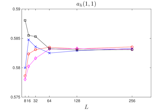
Figure 1. Finite domain approximation to the homogenized coefficient. Different lines correspond to different independent realization of the coefficient field $a$.

We now consider our algorithm to approximate $\nabla u(0)$ based on the $a|_{Q_{2L}}$. To validate the algorithm, we check the numerical convergence rate and compare it with two approximations that with a slower convergence rate. Recall that our algorithms consists of the steps:

• Solve the equation (18) for approximate correctors $\phi^{(L)}_{i}$;

• calculate the homogenized coefficient $a^{(L)}_{h}$ as in (21);

• obtain $u^{(L)}_{h}$ from the homogenized equation (22) and the dipole correction (23);

• solve the equation (25) for $u^{(L)}$.

In comparison, we consider two other algorithms: 1) Solving the equation with homogeneous Dirichlet boundary condition, ie (3), referred as “Dirichlet algorithm”; 2) Dropping the dipole correction, ie, instead of (25), one solves (10) using approximate homogenized coefficient and correctors

$$-\nabla\cdot a\nabla u^{(L)}_{II}=\nabla\cdot g\ \text{in}\ Q_{L},\quad u^{(L)}_{II}=(1+\phi^{(L)}_{i}\partial_{i})\tilde{u}^{(L)}_{h}\ \text{on}\ \partial Q_{L}.$$ (67)

Thus in the boundary condition, $u^{(L)}_{h}$ is replaced by $\tilde{u}^{(L)}_{h}$ so the dipole correction is dropped. This will be referred as the “no dipole algorithm”. In Figure 2, we compare the numerical convergence for the three algorithms with two different realization of the random media. The difference $\nabla u^{(2L)}(0)-\nabla u^{(L)}(0)$ is plotted for various $L$ for the three algorithms. As the plot is in loglog scale, a straight line shows algebraic convergence with the slope indicating the convergence rate. We observe from the numerical results that the proposed algorithm achieves almost $O(L^{-3})$ convergence, which is consistent with the theoretical rate $O((\tfrac{\ell}{L})^{2}(\tfrac{1}{L})^{\beta})$ with $\beta$ close to $1$. The wiggled line is due to the randomness of the coefficients added in the annulus $Q_{4L}-Q_{2L}$ when $L$ is doubled. We also observe that the other two algorithms have the slower rate of $O(L^{-2})$, the main reason being that they do not capture the correct dipole in the far field. It can be also seen that by using the information from homogenization, the “no dipole algorithm” indeed reduces the error compared with the simple minded Dirichlet approximation.

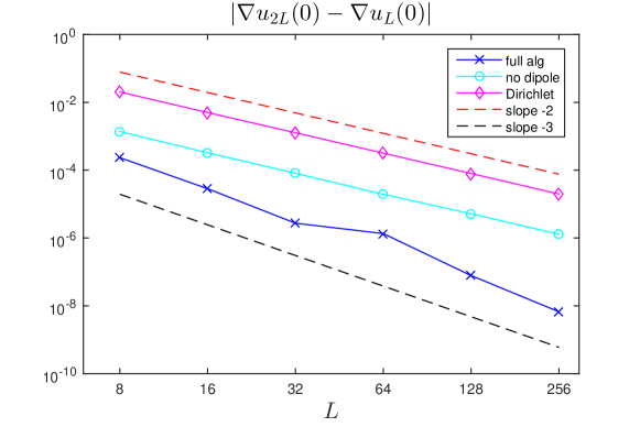
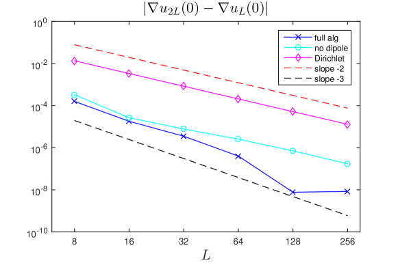
Figure 2. Numerical convergence rate of $\nabla u(0)$ for the proposed algorithm, an approximation without the dipole correction, and the Dirichlet approximation. The two figures correspond to two independent realization of the random medium.

Finally, we study the error committed by the proposed algorithm with the uncertainty of $\nabla u(0)$ due to the unknown coefficient outside $Q_{2L}$. In the second row of Table 1, we compare the approximation $\nabla u^{(L)}(0)$ with the reference solution obtained by a calculation with a large domain ($L=768$ is chosen). In the remaining rows, we show how $\nabla u(0)$ varies when we re-sample the random medium outside $Q_{2L}$ (where again, we take $\nabla u^{(768)}(0)$ as a proxy for $\nabla u(0)$). These thus show the sensitivity of $\nabla u(0)$ with respect to the change of the media. We observe from the numerical results that while the error made by our algorithm is larger than the typical fluctuations of $\nabla u(0)$, the decay rate matches and the error is also comparable to the sensitivity for various $L$.

	$L=32$	$L=64$	$L=128$	$L=256$
$\lvert\nabla u^{(L)}(0)-\nabla u^{(768)}(0)\rvert$	$2.7709\text{\times}{10}^{-6}$	$1.2843\text{\times}{10}^{-6}$	$8.3910\text{\times}{10}^{-8}$	$5.8996\text{\times}{10}^{-9}$
$\nabla u(0)$ difference with re-sampled media in $Q_{2L}^{c}$	$4.8919\text{\times}{10}^{-8}$	$7.7095\text{\times}{10}^{-9}$	$4.9692\text{\times}{10}^{-9}$	$7.8225\text{\times}{10}^{-10}$
	$5.3976\text{\times}{10}^{-8}$	$1.9546\text{\times}{10}^{-8}$	$8.6449\text{\times}{10}^{-9}$	$6.7321\text{\times}{10}^{-10}$
	$1.8771\text{\times}{10}^{-7}$	$3.1458\text{\times}{10}^{-8}$	$1.0232\text{\times}{10}^{-8}$	$5.9754\text{\times}{10}^{-10}$

Table 1. The error of the proposed numerical scheme compared with sensitivity of $\nabla u(0)$ when the media is re-sampled outside $Q_{2L}$. Reference value $\lvert\nabla u^{(768)}(0)\rvert=$3.5859\text{\times}{10}^{-1}$$.

3. Proofs

Proof of Lemma 1.

We start with the remark that (16) actually implies (17). Indeed, what separates (17) from (16) is

$$|\mathchoice{{\vbox{\hbox{$\textstyle-$ }}\kern-7.83337pt}}{{\vbox{\hbox{$\scriptstyle-$ }}\kern-5.90005pt}}{{\vbox{\hbox{$\scriptscriptstyle-$ }}\kern-4.75003pt}}{{\vbox{\hbox{$\scriptscriptstyle-$ }}\kern-4.25003pt}}\!\int_{B_{r}}(\phi,\sigma)-\mathchoice{{\vbox{\hbox{$\textstyle-$ }}\kern-7.83337pt}}{{\vbox{\hbox{$\scriptstyle-$ }}\kern-5.90005pt}}{{\vbox{\hbox{$\scriptscriptstyle-$ }}\kern-4.75003pt}}{{\vbox{\hbox{$\scriptscriptstyle-$ }}\kern-4.25003pt}}\!\int_{B_{r^{\prime}}}(\phi,\sigma)|\lesssim r(\frac{r_{*}}{r})^{\beta}\quad\mbox{for all}\;r\geq r^{\prime}\geq r_{*}.$$ (68)

Since $\beta<1$, we may apply dyadic decomposition to reduce this to

$$|\mathchoice{{\vbox{\hbox{$\textstyle-$ }}\kern-7.83337pt}}{{\vbox{\hbox{$\scriptstyle-$ }}\kern-5.90005pt}}{{\vbox{\hbox{$\scriptscriptstyle-$ }}\kern-4.75003pt}}{{\vbox{\hbox{$\scriptscriptstyle-$ }}\kern-4.25003pt}}\!\int_{B_{r}}(\phi,\sigma)-\mathchoice{{\vbox{\hbox{$\textstyle-$ }}\kern-7.83337pt}}{{\vbox{\hbox{$\scriptstyle-$ }}\kern-5.90005pt}}{{\vbox{\hbox{$\scriptscriptstyle-$ }}\kern-4.75003pt}}{{\vbox{\hbox{$\scriptscriptstyle-$ }}\kern-4.25003pt}}\!\int_{B_{r^{\prime}}}(\phi,\sigma)|\lesssim r(\frac{r_{*}}{r})^{\beta}\quad\mbox{for all}\;2r^{\prime}\geq r\geq r^{\prime}\geq r_{*},$$

which by the triangle inequality is a consequence of (16). In view of (17), we may change $(\phi,\sigma)$ by an additive constant, and thus without affecting (13) to upgrade (16) to

$$\frac{1}{r}\big{(}\mathchoice{{\vbox{\hbox{$\textstyle-$ }}\kern-7.83337pt}}{{\vbox{\hbox{$\scriptstyle-$ }}\kern-5.90005pt}}{{\vbox{\hbox{$\scriptscriptstyle-$ }}\kern-4.75003pt}}{{\vbox{\hbox{$\scriptscriptstyle-$ }}\kern-4.25003pt}}\!\int_{B_{r}}|(\phi,\sigma)|^{2}\big{)}^{\frac{1}{2}}\lesssim(\frac{r_{*}}{r})^{\beta}\quad\mbox{for all}\;r\geq r_{*}.$$ (69)

This is in line with (30).

For later reference we also note that

$$\big{(}\mathchoice{{\vbox{\hbox{$\textstyle-$ }}\kern-7.83337pt}}{{\vbox{\hbox{$\scriptstyle-$ }}\kern-5.90005pt}}{{\vbox{\hbox{$\scriptscriptstyle-$ }}\kern-4.75003pt}}{{\vbox{\hbox{$\scriptscriptstyle-$ }}\kern-4.25003pt}}\!\int_{B_{R}}|e_{i}+\nabla\phi_{i}|^{2}\big{)}^{\frac{1}{2}}\lesssim 1\quad\mbox{for}\;R\geq r_{*},$$ (70)

which is a consequence of Caccioppoli’s estimate on the $a$-harmonic function $x_{i}+\phi_{i}$, cf (5), and (69) in form of $\big{(}\mathchoice{{\vbox{\hbox{$\textstyle-$ }}\kern-7.83337pt}}{{\vbox{\hbox{$\scriptstyle-$ }}\kern-5.90005pt}}{{\vbox{\hbox{$\scriptscriptstyle-$ }}\kern-4.75003pt}}{{\vbox{\hbox{$\scriptscriptstyle-$ }}\kern-4.25003pt}}\!\int_{B_{R}}(x_{i}+\phi_{i})^{2}\big{)}^{\frac{1}{2}}$ $\lesssim R(\frac{r_{*}}{R})^{\beta}$.

We now follow the steps of the proof of [BellaGiuntiOttoPCMINotes, Theorem 0.2] and like there may wlog assume that $r_{*}=1$. In analogy to Step 2 in the proof of [BellaGiuntiOttoPCMINotes, Theorem 0.2] we claim

$$\big{(}\int|\nabla u|^{2}\big{)}^{\frac{1}{2}}\lesssim\ell^{\frac{d}{2}},$$ (71)

and

$$|x|^{d}|\nabla u_{h}(x)|+|x|^{d+1}|\nabla^{2}u_{h}(x)|\lesssim\ell^{d}\quad\mbox{for all}\;x\not=0.$$ (72)

We furthermore claim that the $u$ and $u_{h}$ have not only vanishing “constant invariant”

$$\int\nabla\eta_{r}\cdot a\nabla u=\int\nabla\eta_{r}\cdot a_{h}\nabla u_{h}=0\quad\mbox{for}\;r\geq\ell,$$ (73)

but also identical “linear invariants”, that is,

$$\int\nabla\eta_{r}\cdot((x_{i}+\phi_{i})a\nabla u-ua(e_{i}+\nabla\phi_{i}))$$

$$=\int\nabla\eta_{r}\cdot(x_{i}a_{h}\nabla u_{h}-u_{h}a_{h}e_{i})\quad\mbox{for}\;r\geq\ell,$$ (74)

where $\eta_{r}(x)=\eta(\frac{x}{r})$, and $\eta$ is a cut-off function for $B_{1}$ in $B_{2}$. Indeed, (71) follows from the energy estimate for (2) and the form (4) of the rhs. By the triangle inequality, we split (72) into the corresponding estimate for $\tilde{u}_{h}$ and for $\delta u_{h}:=\xi_{i}\partial_{i}G_{h}$ with $\xi_{i}:=\int\nabla\phi_{i}\cdot g$. We first turn to $\tilde{u}_{h}$ defined through (9) which in view of (4) is of the form $\nabla\tilde{u}_{h}(x)=\hat{\nabla}\hat{u}_{h}(\frac{x}{\ell})$ with $-\hat{\nabla}\cdot a_{h}\hat{\nabla}\hat{u}_{h}$ $=\hat{\nabla}\cdot\hat{g}$, so that the desired estimate follows from

$$|\hat{\nabla}\hat{u}_{h}|\lesssim\frac{1}{|\hat{x}|^{d}+1}\quad\mbox{and}\quad|\hat{\nabla}^{2}\hat{u}_{h}|\lesssim\frac{1}{|\hat{x}|^{d+1}+1},$$

which in turn are a consequence of standard Schauder theory based on the Hölder continuity of $\hat{\nabla}\cdot\hat{g}$ for the near-field, and the Green’s function representation for the far-field. We now turn to $\delta u_{h}$ and note that the estimates

$$|\nabla\delta u_{h}|\lesssim\frac{\ell^{d}}{|x|^{d}}\quad\mbox{and}\quad|\nabla^{2}\delta u_{h}|\lesssim\frac{\ell^{d}}{|x|^{d+1}}$$

follow from the homogeneity of $\nabla^{2}G_{h}$ of degree $-d$ and the fact that $|\xi_{i}|\lesssim\int_{B_{\ell}}|\nabla\phi_{i}|$, Jensen’s inequality together with (70). We now turn to (73). The identity for $u$ follows directly from (2) and the fact that $g$ is supported in $B_{\ell}$, cf (4). For the same reason, the contribution to the constant invariant of $u_{h}$ coming from $\tilde{u}_{h}$ vanishes; the one coming from $\delta u_{h}$, which is constant in $r>0$ by $a_{h}$-harmonicity (thus the name “invariant”), must vanish by its homogeneity of order $1-d$. We finally turn to (3). By (2) and (5) we learn from an integration by parts and the support condition on $g$ that for $r\geq\ell$,

$$\int\nabla\eta_{r}\cdot((x_{i}+\phi_{i})a\nabla u-ua(e_{i}+\nabla\phi_{i}))=\int(e_{i}+\nabla\phi_{i})\cdot g.$$ (75)

Likewise, we obtain from (9) that

$$\int\nabla\eta_{r}\cdot(x_{i}a_{h}\nabla\tilde{u}_{h}-\tilde{u}_{h}a_{h}e_{i})=\int e_{i}\cdot g.$$

Finally, by definition of the Green’s function $G_{h}$ we have

$$\int\nabla\eta_{r}\cdot(x_{i}a_{h}\nabla\partial_{j}G_{h}-\partial_{j}G_{h}a_{h}e_{i})=\delta_{ij}.$$

By $u_{h}=\tilde{u}_{h}+\xi_{j}\partial_{j}G_{h}$ and the definition of $\xi$, the last two identities combine to

$$\int\nabla\eta_{r}\cdot((x_{i}a_{h}\nabla u_{h}-u_{h}a_{h}e_{i})=\int(e_{i}+\nabla\phi_{i})\cdot g.$$

This and (75) yield the identity (3).

Following Step 3 in the proof of [BellaGiuntiOttoPCMINotes, Theorem 0.2] (with $\eta=0$, the additional multiplicative factor $\ell^{d}$, and $\beta$ playing the role of $1-\alpha$) we consider the error in the two-scale expansion $w:=u-(1+\phi_{i}\partial_{i})u_{h}$ we claim that

$$\big{(}\int_{B_{1}^{c}}|\nabla w|^{2}\big{)}^{\frac{1}{2}}\lesssim\ell^{d}$$ (76)

and that

$$-\nabla\cdot a\nabla w=\nabla\cdot h\quad\mbox{with}\quad h:=(\phi_{i}a-\sigma_{i})\nabla\partial_{i}u_{h},$$ (77)

where

$$\big{(}\frac{1}{R^{d}}\int_{B_{r}^{c}}|h|^{2}\big{)}^{\frac{1}{2}}\lesssim\ell^{d}(\frac{1}{r})^{d+\beta}\quad\mbox{for}\;r\geq 1.$$ (78)

We first turn to (76) and note $\nabla w=\nabla u-\partial_{i}u_{h}(e_{i}+\nabla\phi_{i})-\phi_{i}\nabla\partial_{i}u_{h}$. Hence for the $\nabla u$-contribution the desired estimate follows from (71) (and $\ell\geq 1$). According to (72), the contribution from $\partial_{i}u_{h}(e_{i}+\nabla\phi_{i})$ is estimated by $\ell^{d}\big{(}\int_{B_{1}^{c}}|x|^{-2d}|e_{i}+\nabla\phi_{i}|^{2}\big{)}^{\frac{1}{2}}$; dividing the integral into dyadic annuli and using (70), we see that it is $\lesssim 1$. Still according to (72), the contribution from $\phi_{i}\nabla\partial_{i}u_{h}$ is estimated by $\ell^{d}\big{(}\int_{B_{1}^{c}}|x|^{-2(d+1)}\phi_{i}^{2}\big{)}^{\frac{1}{2}}$; dividing also this integral into dyadic annuli and using (69), we see that it is $\lesssim 1$. As $-\nabla\cdot a\nabla u=\nabla\cdot g=\nabla\cdot a_{h}\nabla u_{h}$ (in view of (2), (9), and the $a_{h}$-harmonicity of $G_{h}$ and thus $\delta u_{h}$ away from the origin), the identity (77) follows by a straightforward calculation as in Step 3 of [BellaGiuntiOttoPCMINotes]. It is the merit of $\sigma_{i}$ that the rhs can be written in divergence-form $\nabla\cdot h$. We finally turn to the estimate (78); by (72) and (1) we have $|h|\lesssim\ell^{d}|x|^{-(d+1)}|(\phi,\sigma)|$. Hence the estimate follows once more from (69) and division into dyadic annuli.

Following Step 4 and Step 5 of [BellaGiuntiOttoPCMINotes, Theorem 0.2] (still with $\alpha$ replaced by $1-\beta$ and the additional factor of $\ell^{d}$) we obtain

$$\big{(}\frac{1}{R^{d}}\int_{B_{r}^{c}}|\nabla w|^{2}\big{)}^{\frac{1}{2}}\lesssim\ell^{d}(\frac{1}{r})^{d+\beta}\quad\mbox{for}\;r\geq 2,$$

which (in view of $r_{*}=1$) turns into (29). Note that the outcome of Step 5 of [BellaGiuntiOttoPCMINotes, Theorem 0.2] is worse by a $\log R$; which however can be easily avoided, cf [BellaGiuntiOttoarXiv, Lemma 3] with $k=1$ and $r=r_{*}=1$.

∎

Proof of Corollary 1.

Let us introduce a tool we will often use, namely the $C^{0,1}$-estimate for an $a$-harmonic function $w$ in $B_{R}$, the crucial role of which was recognized in [AS]. As is obvious from its characterization (16), $r_{*}$ dominates, up to a multiplicative constant $C=C(d,\lambda,\beta)$, the “minimal radius” introduced in [GNOarXiv] and from which on the “mean-value property”, as an estimate, holds for $|\nabla w|^{2}$, see [GNOarXiv, Theorem 1] for the proof. We record this

$$\mathchoice{{\vbox{\hbox{$\textstyle-$ }}\kern-7.83337pt}}{{\vbox{\hbox{$\scriptstyle-$ }}\kern-5.90005pt}}{{\vbox{\hbox{$\scriptscriptstyle-$ }}\kern-4.75003pt}}{{\vbox{\hbox{$\scriptscriptstyle-$ }}\kern-4.25003pt}}\!\int_{B_{r}}|\nabla w|^{2}\leq C(d,\lambda,\beta)\mathchoice{{\vbox{\hbox{$\textstyle-$ }}\kern-7.83337pt}}{{\vbox{\hbox{$\scriptstyle-$ }}\kern-5.90005pt}}{{\vbox{\hbox{$\scriptscriptstyle-$ }}\kern-4.75003pt}}{{\vbox{\hbox{$\scriptscriptstyle-$ }}\kern-4.25003pt}}\!\int_{B_{R}}|\nabla w|^{2}\quad\mbox{for}\;r_{*}\leq r\leq R.$$ (79)

We note that the combination of (9), (11) and (12) may be rephrased in terms of $w:=u_{III}-u$ and $w_{D}:=u-(1+\phi_{i}\partial_{i})u_{h}$ as

$$-\nabla\cdot a\nabla w=0\;\mbox{in}\;Q_{L}\quad\mbox{and}\quad w=w_{D}\;\mbox{on}\;\partial Q_{L}.$$ (80)

Once we show that this implies

$$\big{(}\int_{Q_{L}}|\nabla w|^{2}\big{)}^{\frac{1}{2}}\lesssim\big{(}\int_{Q_{2L}-Q_{L}}|\nabla w_{D}|^{2}\big{)}^{\frac{1}{2}},$$ (81)

we see that (31) follows from (29) for $R=L$, and a subsequent application of the $C^{0,1}$-estimate for $w$ to get from $Q_{L}$ to $B_{R}$ for $R\geq r_{*}$.

We now turn to the argument that (80) implies (81) under the mere assumption of uniform ellipticity, cf (1). Hence by rescaling, we may wlog assume $L=1$. Since (80) and (81) are oblivious to additive constant we may wlog assume $\int_{Q_{2}-Q_{1}}w_{D}=0$, which allows to construct an extension $\bar{w}_{D}$ of $w_{D}$ on $Q_{1}$ such that

$$\big{(}\int_{Q_{2}}|\nabla\bar{w}_{D}|^{2}\big{)}^{\frac{1}{2}}\lesssim\big{(}\int_{Q_{2}-Q_{1}}|\nabla w_{D}|^{2}\big{)}^{\frac{1}{2}}.$$ (82)

This extension allows us to reformulate (80) as

$$-\nabla\cdot a\nabla(w-\bar{w}_{D})=\nabla\cdot a\nabla\bar{w}_{D}\;\mbox{in}\;Q_{1},\quad w-\bar{w}_{D}=0\;\mbox{on}\;\partial Q_{1}.$$

Hence (81) follows by the energy estimate on the latter, followed by a triangle inequality in $L^{2}$ yielding $\big{(}\int_{Q_{1}}|\nabla w|^{2}\big{)}^{\frac{1}{2}}$ $\lesssim\big{(}\int_{Q_{1}}|\nabla\bar{w}_{D}|^{2}\big{)}^{\frac{1}{2}}$, into which we insert (82). ∎

Proof of Lemma 2.

We first turn to (33) and, for notational simplicity, drop the index $i=1,\cdots,d$. By (5), which is as mentioned a consequence of (13), and (18) we have $-\nabla\cdot a\nabla(\phi^{(L)}-\phi)$ $=0$ in $Q_{2L}$, so that by Caccioppoli’s estimate and the triangle inequality in $L^{2}$ we have

$$\big{(}\mathchoice{{\vbox{\hbox{$\textstyle-$ }}\kern-7.83337pt}}{{\vbox{\hbox{$\scriptstyle-$ }}\kern-5.90005pt}}{{\vbox{\hbox{$\scriptscriptstyle-$ }}\kern-4.75003pt}}{{\vbox{\hbox{$\scriptscriptstyle-$ }}\kern-4.25003pt}}\!\int_{Q_{\frac{3}{2}L}} |\nabla(\phi^{(L)}-\phi)|^{2}\big{)}^{\frac{1}{2}}\lesssim\frac{1}{L}\big{(}\mathchoice{{\vbox{\hbox{$\textstyle-$ }}\kern-7.83337pt}}{{\vbox{\hbox{$\scriptstyle-$ }}\kern-5.90005pt}}{{\vbox{\hbox{$\scriptscriptstyle-$ }}\kern-4.75003pt}}{{\vbox{\hbox{$\scriptscriptstyle-$ }}\kern-4.25003pt}}\!\int_{Q_{2L}}((\phi^{(L)}-\phi)-\mathchoice{{\vbox{\hbox{$\textstyle-$ }}\kern-7.83337pt}}{{\vbox{\hbox{$\scriptstyle-$ }}\kern-5.90005pt}}{{\vbox{\hbox{$\scriptscriptstyle-$ }}\kern-4.75003pt}}{{\vbox{\hbox{$\scriptscriptstyle-$ }}\kern-4.25003pt}}\!\int_{Q_{2L}}\phi)^{2}\big{)}^{\frac{1}{2}}$$

$$\leq\frac{1}{L}\big{(}\mathchoice{{\vbox{\hbox{$\textstyle-$ }}\kern-7.83337pt}}{{\vbox{\hbox{$\scriptstyle-$ }}\kern-5.90005pt}}{{\vbox{\hbox{$\scriptscriptstyle-$ }}\kern-4.75003pt}}{{\vbox{\hbox{$\scriptscriptstyle-$ }}\kern-4.25003pt}}\!\int_{Q_{2L}}(\phi^{(L)})^{2}\big{)}^{\frac{1}{2}}+\frac{1}{L}\big{(}\mathchoice{{\vbox{\hbox{$\textstyle-$ }}\kern-7.83337pt}}{{\vbox{\hbox{$\scriptstyle-$ }}\kern-5.90005pt}}{{\vbox{\hbox{$\scriptscriptstyle-$ }}\kern-4.75003pt}}{{\vbox{\hbox{$\scriptscriptstyle-$ }}\kern-4.25003pt}}\!\int_{Q_{2L}}(\phi-\mathchoice{{\vbox{\hbox{$\textstyle-$ }}\kern-7.83337pt}}{{\vbox{\hbox{$\scriptstyle-$ }}\kern-5.90005pt}}{{\vbox{\hbox{$\scriptscriptstyle-$ }}\kern-4.75003pt}}{{\vbox{\hbox{$\scriptscriptstyle-$ }}\kern-4.25003pt}}\!\int_{Q_{2L}}\phi)^{2}\big{)}^{\frac{1}{2}}.$$

Hence (33) follows from the $\phi$-parts in (27) and (32) .

For (34), we argue in a similar way: According to (13), which yields (14), and (19) we have $-\Delta(\sigma^{(L)}_{jk}-\sigma_{jk})$ $=\partial_{j}(q^{(L)}_{k}-q_{k})-\partial_{k}(q^{(L)}_{j}-q_{j})$ in $Q_{2L}$, where we recall $q=a(e+\nabla\phi)$, $q^{(L)}=a(e+\nabla\phi^{(L)})$ and thus $q^{(L)}-q=a\nabla(\phi^{(L)}-\phi)$. By Caccioppoli’s estimate and the upper bound on $a$ provided by (1) we therefore obtain

$$\big{(}\mathchoice{{\vbox{\hbox{$\textstyle-$ }}\kern-7.83337pt}}{{\vbox{\hbox{$\scriptstyle-$ }}\kern-5.90005pt}}{{\vbox{\hbox{$\scriptscriptstyle-$ }}\kern-4.75003pt}}{{\vbox{\hbox{$\scriptscriptstyle-$ }}\kern-4.25003pt}}\!\int_{Q_{L}}|\nabla(\sigma^{(L)}-\sigma)|^{2}\big{)}^{\frac{1}{2}}$$

$$\lesssim\big{(}\mathchoice{{\vbox{\hbox{$\textstyle-$ }}\kern-7.83337pt}}{{\vbox{\hbox{$\scriptstyle-$ }}\kern-5.90005pt}}{{\vbox{\hbox{$\scriptscriptstyle-$ }}\kern-4.75003pt}}{{\vbox{\hbox{$\scriptscriptstyle-$ }}\kern-4.25003pt}}\!\int_{Q_{\frac{3}{2}L}}|\nabla(\phi^{(L)}-\phi)|^{2}\big{)}^{\frac{1}{2}}+\frac{1}{L}\big{(}\mathchoice{{\vbox{\hbox{$\textstyle-$ }}\kern-7.83337pt}}{{\vbox{\hbox{$\scriptstyle-$ }}\kern-5.90005pt}}{{\vbox{\hbox{$\scriptscriptstyle-$ }}\kern-4.75003pt}}{{\vbox{\hbox{$\scriptscriptstyle-$ }}\kern-4.25003pt}}\!\int_{Q_{2L}}|\sigma^{(L)}|^{2}\big{)}^{\frac{1}{2}}+\frac{1}{L}\big{(}\mathchoice{{\vbox{\hbox{$\textstyle-$ }}\kern-7.83337pt}}{{\vbox{\hbox{$\scriptstyle-$ }}\kern-5.90005pt}}{{\vbox{\hbox{$\scriptscriptstyle-$ }}\kern-4.75003pt}}{{\vbox{\hbox{$\scriptscriptstyle-$ }}\kern-4.25003pt}}\!\int_{Q_{2L}}|\sigma-\mathchoice{{\vbox{\hbox{$\textstyle-$ }}\kern-7.83337pt}}{{\vbox{\hbox{$\scriptstyle-$ }}\kern-5.90005pt}}{{\vbox{\hbox{$\scriptscriptstyle-$ }}\kern-4.75003pt}}{{\vbox{\hbox{$\scriptscriptstyle-$ }}\kern-4.25003pt}}\!\int_{Q_{2L}}\sigma|^{2}\big{)}^{\frac{1}{2}}.$$

Hence (34) follows from (33) and the $\sigma$-parts of both (27) and (32).

We now turn to (35) and recall our averaging function $\omega$, cf (20). We first claim that also for the whole-space case, the effective coefficient can approximately be recovered from averaging the flux wrt to $\omega$:

$$|a_{h}e-\int\omega a(e+\nabla\phi)|\lesssim(\frac{r_{*}}{L})^{\beta}.$$ (83)

The argument for this is based on (13), which yields the identity $a_{h}e-\int\omega a(e+\nabla\phi)$ $=\int(\sigma-\mathchoice{{\vbox{\hbox{$\textstyle-$ }}\kern-7.83337pt}}{{\vbox{\hbox{$\scriptstyle-$ }}\kern-5.90005pt}}{{\vbox{\hbox{$\scriptscriptstyle-$ }}\kern-4.75003pt}}{{\vbox{\hbox{$\scriptscriptstyle-$ }}\kern-4.25003pt}}\!\int_{B_{L}}\sigma)$ $\nabla\omega$, and thus by (20) the estimate $|a_{h}e$ $-\int\omega a(e+\nabla\phi)|$ $\lesssim\frac{1}{L}\mathchoice{{\vbox{\hbox{$\textstyle-$ }}\kern-7.83337pt}}{{\vbox{\hbox{$\scriptstyle-$ }}\kern-5.90005pt}}{{\vbox{\hbox{$\scriptscriptstyle-$ }}\kern-4.75003pt}}{{\vbox{\hbox{$\scriptscriptstyle-$ }}\kern-4.25003pt}}\!\int_{B_{L}}|\sigma-\mathchoice{{\vbox{\hbox{$\textstyle-$ }}\kern-7.83337pt}}{{\vbox{\hbox{$\scriptstyle-$ }}\kern-5.90005pt}}{{\vbox{\hbox{$\scriptscriptstyle-$ }}\kern-4.75003pt}}{{\vbox{\hbox{$\scriptscriptstyle-$ }}\kern-4.25003pt}}\!\int_{B_{L}}\sigma|$. Hence we obtain (83) from (32) and Jensen’s inequality.

We now may conclude: By the upper bound provided in (1), we obtain from (83) and the definition (21) by the triangle inequality

$$|(a^{(L)}_{h}-a_{h})e|\lesssim\mathchoice{{\vbox{\hbox{$\textstyle-$ }}\kern-7.83337pt}}{{\vbox{\hbox{$\scriptstyle-$ }}\kern-5.90005pt}}{{\vbox{\hbox{$\scriptscriptstyle-$ }}\kern-4.75003pt}}{{\vbox{\hbox{$\scriptscriptstyle-$ }}\kern-4.25003pt}}\!\int_{Q_{L}}|\nabla(\phi^{(L)}-\phi)|+(\frac{r_{*}}{L})^{\beta},$$

so that (35) follows from (33) and Jensen’s inequality. ∎

Proof of Proposition 1.

We first compare the two solutions $\tilde{u}^{(L)}_{h}$ and $\tilde{u}_{h}$ of (22) and (9), respectively, and claim that

$$|\nabla(\tilde{u}^{(L)}_{h}-\tilde{u}_{h})|+L|\nabla^{2}(\tilde{u}^{(L)}_{h}-\tilde{u}_{h})|\lesssim(\frac{r_{*}}{L})^{\beta}(\frac{\ell}{L})^{d}\quad\mbox{on}\;Q_{L}^{c}.$$ (84)

Indeed, the difference $w:=\tilde{u}^{(L)}_{h}-\tilde{u}_{h}$ satisfies

$$-\nabla\cdot a^{(L)}_{h}\nabla w=\nabla\cdot(a^{(L)}_{h}-a_{h})\nabla\tilde{u}_{h}.$$

The form (4) of the rhs $g$ in (9) transmits to the solution $\tilde{u}_{h}$: $\nabla\tilde{u}_{h}(x)$ $=\hat{\nabla}\widehat{\tilde{u}_{h}}(\frac{x}{\ell})$, and then also to $w$: $\nabla w(x)$ $=\hat{\nabla}\hat{w}(\frac{x}{\ell})$. Recall that $\hat{g}$ is compactly supported in $B_{1}$ with Hölder continuous derivatives; in particular, $\hat{g}$ is in the class of vector fields decaying as $O(|x|^{-d})$ with derivatives decaying as $O(|x|^{-d-1})$ and differences of the derivatives decaying as $O(|x|^{-d-1-\alpha}|x-y|^{\alpha})$, in line with $\alpha$-Hölder continuity for some $\alpha\in(0,1)$. This class is preserved under the constant-coefficient Helmholtz projection (recall that $a^{(L)}_{h}$ satisfies (1)). Hence we obtain in particular

$$|\hat{\nabla}\hat{w}|\lesssim|a^{(L)}_{h}-a_{h}|\frac{1}{(|\hat{x}|+1)^{d}}, \quad|\hat{\nabla}^{2}\hat{w}|\lesssim|a^{(L)}_{h}-a_{h}|\frac{1}{(|\hat{x}|+1)^{d+1}}.$$

Translating back to the microscopic variables and using (35) in Lemma 2 we have

$$|\nabla w|\lesssim(\frac{r_{*}}{L})^{\beta}(\frac{\ell}{|x|+\ell})^{d}, \quad\ell|\nabla^{2}w|\lesssim(\frac{r_{*}}{L})^{\beta}(\frac{\ell}{|x|+\ell})^{d+1},$$

from which we extract (84).

We now compare $u^{(L)}_{h}$ and $u_{h}$ defined in (23) and (11) and claim that

$$|\nabla(u^{(L)}_{h}-u_{h})|+L|\nabla^{2}(u^{(L)}_{h}-u_{h})|\lesssim(\frac{r_{*}}{L})^{\beta}(\frac{\ell}{L})^{d}\quad\mbox{on}\;Q_{L}^{c}.$$ (85)

For later purpose, we also record

$$|\nabla u^{(L)}_{h}|+L|\nabla^{2}u^{(L)}_{h}|\lesssim(\frac{\ell}{L})^{d}\quad\mbox{on}\;Q_{L}^{c}.$$ (86)

In order to pass from (84) to (85), and from (72) and (85) to (86), it remains to control the dipole contributions:

$$|\nabla(\xi^{(L)}_{i}\partial_{i}G^{(L)}_{h}-\xi_{i}\partial_{i}G_{h})| +L|\nabla^{2}(\xi^{(L)}_{i}\partial_{i}G^{(L)}_{h}-\xi_{i}\partial_{i}G_{h})|\lesssim(\frac{r_{*}}{L})^{\beta}(\frac{\ell}{L})^{d}$$

$$\mbox{and}\quad|\nabla\xi_{i}\partial_{i}G^{(L)}_{h}| +L|\nabla^{2}\xi_{i}\partial_{i}G^{(L)}_{h}|\lesssim(\frac{\ell}{L})^{d}\quad\mbox{both on}\;Q_{L}^{c},$$

where we have set for abbreviation $\xi^{(L)}_{i}$ $:=\int\nabla\phi^{(L)}_{i}\cdot g$ and (as above) $\xi_{i}=\int\nabla\phi_{i}\cdot g$. Because of the obvious estimates on the constant-coefficient (and thus homogeneous) fundamental solution

$$|\nabla\partial_{i}G^{(L)}_{h}|+L|\nabla^{2}\partial_{i}G^{(L)}_{h}|\lesssim\frac{1}{L^{d}}\quad\mbox{on}\;Q_{L}^{c}$$

and

$$|\nabla\partial_{i}(G^{(L)}_{h}-G_{h})|+L|\nabla^{2}\partial_{i}(G^{(L)}_{h}-G_{h})| \lesssim|a^{(L)}_{h}-a_{h}|\frac{1}{L^{d}}$$

$$\lesssim(\frac{r_{*}}{L})^{\beta}\frac{1}{L^{d}}\quad\mbox{on}\;Q_{L}^{c},$$

it suffices to show

$$|\xi|\lesssim\ell^{d}\quad\mbox{and}\quad|\xi^{(L)}-\xi|\lesssim(\frac{r_{*}}{L})^{\beta}\ell^{d}.$$

By definition of $\xi^{(L)},\xi$, the form (4) of $g$, and Jensen’s inequality the latter two estimates follow from

$$\big{(}\mathchoice{{\vbox{\hbox{$\textstyle-$ }}\kern-7.83337pt}}{{\vbox{\hbox{$\scriptstyle-$ }}\kern-5.90005pt}}{{\vbox{\hbox{$\scriptscriptstyle-$ }}\kern-4.75003pt}}{{\vbox{\hbox{$\scriptscriptstyle-$ }}\kern-4.25003pt}}\!\int_{B_{\ell}}|\nabla\phi|^{2}\big{)}^{\frac{1}{2}}\lesssim 1\quad\mbox{and}\quad\big{(}\mathchoice{{\vbox{\hbox{$\textstyle-$ }}\kern-7.83337pt}}{{\vbox{\hbox{$\scriptstyle-$ }}\kern-5.90005pt}}{{\vbox{\hbox{$\scriptscriptstyle-$ }}\kern-4.75003pt}}{{\vbox{\hbox{$\scriptscriptstyle-$ }}\kern-4.25003pt}}\!\int_{B_{\ell}}|\nabla(\phi^{(L)}-\phi)|^{2}\big{)}^{\frac{1}{2}}\lesssim(\frac{r_{*}}{L})^{\beta}.$$ (87)

The first estimate in (87) follows from (70) since $\ell\geq r_{*}$. The second estimate in (87) follows from (33) in Lemma 2 and the $C^{0,1}$-estimate for an $a$-harmonic function $w$ in $Q_{L}$, cf (79), which requires $L\geq\ell\geq r_{*}$.

We finally compare $u^{(L)}$ defined through (25) with $u_{III}$ defined through (12) and claim that

$$\big{(}\mathchoice{{\vbox{\hbox{$\textstyle-$ }}\kern-7.83337pt}}{{\vbox{\hbox{$\scriptstyle-$ }}\kern-5.90005pt}}{{\vbox{\hbox{$\scriptscriptstyle-$ }}\kern-4.75003pt}}{{\vbox{\hbox{$\scriptscriptstyle-$ }}\kern-4.25003pt}}\!\int_{B_{R}}|\nabla(u^{(L)}-u_{III})|^{2}\big{)}^{\frac{1}{2}}\lesssim(\frac{\ell}{L})^{d}(\frac{r_{*}}{L})^{\beta}\quad\mbox{for}\;L\geq R\geq r_{*}.$$

This allows us to pass from (31) in Corollary 1 to this proposition’s statement (28). We note that because $w:=u^{(L)}-u_{III}$ satisfies

$$-\nabla\cdot a\nabla w=0\quad\mbox{in}\;Q_{L},\quad w=w_{D}\quad\mbox{on}\;\partial Q_{L},$$

where $w_{D}:=(1+\phi^{(L)}_{i}\partial_{i})u^{(L)}_{h}-(1+\phi_{i}\partial_{i})u_{h}$. Hence we have by (a slight adaptation of) the argument at the beginning of the proof of Corollary 1 that

$$\big{(}\mathchoice{{\vbox{\hbox{$\textstyle-$ }}\kern-7.83337pt}}{{\vbox{\hbox{$\scriptstyle-$ }}\kern-5.90005pt}}{{\vbox{\hbox{$\scriptscriptstyle-$ }}\kern-4.75003pt}}{{\vbox{\hbox{$\scriptscriptstyle-$ }}\kern-4.25003pt}}\!\int_{Q_{L}}|\nabla w|^{2}\big{)}^{\frac{1}{2}}\lesssim\big{(}\mathchoice{{\vbox{\hbox{$\textstyle-$ }}\kern-7.83337pt}}{{\vbox{\hbox{$\scriptstyle-$ }}\kern-5.90005pt}}{{\vbox{\hbox{$\scriptscriptstyle-$ }}\kern-4.75003pt}}{{\vbox{\hbox{$\scriptscriptstyle-$ }}\kern-4.25003pt}}\!\int_{Q_{\frac{3}{2}L}-Q_{L}}|\nabla w_{D}|^{2}\big{)}^{\frac{1}{2}}.$$

We combine this with the $C^{0,1}$-estimate, cf (79), for $a$-harmonic functions, so that it remains to show

$$\big{(}\mathchoice{{\vbox{\hbox{$\textstyle-$ }}\kern-7.83337pt}}{{\vbox{\hbox{$\scriptstyle-$ }}\kern-5.90005pt}}{{\vbox{\hbox{$\scriptscriptstyle-$ }}\kern-4.75003pt}}{{\vbox{\hbox{$\scriptscriptstyle-$ }}\kern-4.25003pt}}\!\int_{Q_{\frac{3}{2}L}-Q_{L}}|\nabla w_{D}|^{2}\big{)}^{\frac{1}{2}}\lesssim(\frac{\ell}{L})^{d}(\frac{r_{*}}{L})^{\beta}.$$ (88)

We appeal to the triangle inequality in $L^{2}$ to split $\nabla w_{D}$ into the four contributions

$$\nabla w_{D} =\partial_{i}(u^{(L)}_{h}-u_{h})(e_{i}+\nabla\phi_{i})+\phi_{i}\nabla\partial_{i}(u^{(L)}_{h}-u_{h})$$

$$+\partial_{i}u^{(L)}_{h}\nabla(\phi^{(L)}_{i}-\phi_{i})+(\phi^{(L)}_{i}-\phi_{i})\nabla\partial_{i}u^{(L)}_{h}.$$

For the first contribution, (88) follows from the first part of (85) and (70). For the second contribution, (88) follows from the second part of (85) and (69), recall the normalization of $\phi_{i}$ through $\mathchoice{{\vbox{\hbox{$\textstyle-$ }}\kern-7.83337pt}}{{\vbox{\hbox{$\scriptstyle-$ }}\kern-5.90005pt}}{{\vbox{\hbox{$\scriptscriptstyle-$ }}\kern-4.75003pt}}{{\vbox{\hbox{$\scriptscriptstyle-$ }}\kern-4.25003pt}}\!\int_{B_{r_{*}}}\phi_{i}=0$, cf (30). For the third contribution, we appeal to the first part of (86) and (33). For the fourth contribution we appeal once more to (69), and now also to (27), which we combine to $\big{(}\mathchoice{{\vbox{\hbox{$\textstyle-$ }}\kern-7.83337pt}}{{\vbox{\hbox{$\scriptstyle-$ }}\kern-5.90005pt}}{{\vbox{\hbox{$\scriptscriptstyle-$ }}\kern-4.75003pt}}{{\vbox{\hbox{$\scriptscriptstyle-$ }}\kern-4.25003pt}}\!\int_{Q_{\frac{3}{2}L}}(\phi^{(L)}_{i}-\phi_{i})^{2}\big{)}^{\frac{1}{2}}$ $\lesssim L(\frac{r_{*}}{L})^{\beta}$. In connection with the second part of (86), we see that also that this last contribution is controlled as stated in (88). ∎

Proof of Lemma 3.

As mentioned in the introduction, (18) and (19) do not ensure the analogue of (13), that is, $q^{(L)}_{i}$ $:=a(e_{i}+\nabla\phi^{(L)}_{i})$ $=a^{(L)}_{h}e_{i}+\nabla\cdot\sigma^{(L)}_{i}$. However, we will need the $C^{1,\alpha}$-theory for $a$ from [GNOarXiv, Theorem 1] on scales $\frac{L}{2}\geq r\geq r^{(L)}_{*}$, which relies on this identity next to the controlled sublinearity (24). Hence for arbitrary but fixed $i=1,\cdots,d$, we need to modify $\sigma^{(L)}_{i}$ to (a still skew symmetric) $\tilde{\sigma}_{i}$ with

$$q^{(L)}_{i}=a^{(L)}_{h}e_{i}+\nabla\cdot\tilde{\sigma}_{i}\quad\mbox{on}\;Q_{L},$$ (89)

while retaining the $\sigma$-part of (24) in (the seemingly weaker) form of

$$\frac{1}{r}\big{(}\mathchoice{{\vbox{\hbox{$\textstyle-$ }}\kern-7.83337pt}}{{\vbox{\hbox{$\scriptstyle-$ }}\kern-5.90005pt}}{{\vbox{\hbox{$\scriptscriptstyle-$ }}\kern-4.75003pt}}{{\vbox{\hbox{$\scriptscriptstyle-$ }}\kern-4.25003pt}}\!\int_{Q_{r}}|\tilde{\sigma}_{i}-\mathchoice{{\vbox{\hbox{$\textstyle-$ }}\kern-7.83337pt}}{{\vbox{\hbox{$\scriptstyle-$ }}\kern-5.90005pt}}{{\vbox{\hbox{$\scriptscriptstyle-$ }}\kern-4.75003pt}}{{\vbox{\hbox{$\scriptscriptstyle-$ }}\kern-4.25003pt}}\!\int_{Q_{r}}\tilde{\sigma}_{i}|^{2}\big{)}^{\frac{1}{2}}\lesssim(\frac{r^{(L)}_{*}}{r})^{\beta}\quad\mbox{for}\;L\geq r\geq r^{(L)}_{*}.$$ (90)

To this purpose, we first argue that the “defect” $g^{(L)}_{i}:=q^{(L)}_{i}-a^{(L)}_{h}e_{i}-\nabla\cdot\sigma^{(L)}_{i}$, which as mentioned in the introduction is component-wise harmonic on $Q_{2L}$ by (18) and (19), satisfies

$$\big{(}\mathchoice{{\vbox{\hbox{$\textstyle-$ }}\kern-7.83337pt}}{{\vbox{\hbox{$\scriptstyle-$ }}\kern-5.90005pt}}{{\vbox{\hbox{$\scriptscriptstyle-$ }}\kern-4.75003pt}}{{\vbox{\hbox{$\scriptscriptstyle-$ }}\kern-4.25003pt}}\!\int_{Q_{L}}|g^{(L)}_{i}|^{2}\big{)}^{\frac{1}{2}}\lesssim(\frac{r^{(L)}_{*}}{L})^{\beta}.$$ (91)

Indeed, this follows immediately from the identity (13) in conjunction with the three estimates (33), (34), and (35) in Lemma 2 (applied with $r_{*}$ replaced by $r^{(L)}_{*}$).

We now turn to (89) and (90). In view of the definition of the defect $g^{(L)}_{i}$, Poincaré’s inequality, and (24), it is enough to construct $\delta\tilde{\sigma}_{i}$ such that

$$g^{(L)}_{i}=\nabla\cdot\delta\tilde{\sigma}_{i}\quad\mbox{on}\;Q_{L}$$ (92)

and

$$\big{(}\mathchoice{{\vbox{\hbox{$\textstyle-$ }}\kern-7.83337pt}}{{\vbox{\hbox{$\scriptstyle-$ }}\kern-5.90005pt}}{{\vbox{\hbox{$\scriptscriptstyle-$ }}\kern-4.75003pt}}{{\vbox{\hbox{$\scriptscriptstyle-$ }}\kern-4.25003pt}}\!\int_{Q_{r}}|\nabla\delta\tilde{\sigma}_{i}|^{2}\big{)}^{\frac{1}{2}}\lesssim(\frac{r^{(L)}_{*}}{L})^{\beta}\quad\mbox{for}\;L\geq r\geq r^{(L)}_{*}.$$ (93)

To this purpose, we extend the restriction of $g^{(L)}_{i}$ to $Q_{L}$ periodically (without changing the notation) and let $\delta\sigma^{(L)}_{i}$ be the $Q_{L}$-periodic solution of

$$-\Delta\delta\sigma^{(L)}_{ijk}=\partial_{j}g^{(L)}_{ik}-\partial_{k}g^{(L)}_{ij}\quad\mbox{with}\quad\mathchoice{{\vbox{\hbox{$\textstyle-$ }}\kern-7.83337pt}}{{\vbox{\hbox{$\scriptstyle-$ }}\kern-5.90005pt}}{{\vbox{\hbox{$\scriptscriptstyle-$ }}\kern-4.75003pt}}{{\vbox{\hbox{$\scriptscriptstyle-$ }}\kern-4.25003pt}}\!\int_{Q_{L}}\delta\sigma^{(L)}_{ijk}=0.$$ (94)

By a remark in the introduction, periodic boundary conditions ensure

$$g^{(L)}_{i}-\mathchoice{{\vbox{\hbox{$\textstyle-$ }}\kern-7.83337pt}}{{\vbox{\hbox{$\scriptstyle-$ }}\kern-5.90005pt}}{{\vbox{\hbox{$\scriptscriptstyle-$ }}\kern-4.75003pt}}{{\vbox{\hbox{$\scriptscriptstyle-$ }}\kern-4.25003pt}}\!\int_{Q_{L}}g^{(L)}_{i}=\nabla\cdot\delta\sigma^{(L)}_{i}.$$ (95)

We claim that (93) holds for $\delta\sigma^{(L)}_{i}$:

$$\big{(}\mathchoice{{\vbox{\hbox{$\textstyle-$ }}\kern-7.83337pt}}{{\vbox{\hbox{$\scriptstyle-$ }}\kern-5.90005pt}}{{\vbox{\hbox{$\scriptscriptstyle-$ }}\kern-4.75003pt}}{{\vbox{\hbox{$\scriptscriptstyle-$ }}\kern-4.25003pt}}\!\int_{Q_{r}}|\nabla\delta\sigma^{(L)}_{i}|^{2}\big{)}^{\frac{1}{2}}\lesssim(\frac{r^{(L)}_{*}}{L})^{\beta}\quad\mbox{for}\;L\geq r\geq r^{(L)}_{*}.$$ (96)

Indeed, since by the energy estimate for the periodic problem (94), that is,

$$\big{(}\mathchoice{{\vbox{\hbox{$\textstyle-$ }}\kern-7.83337pt}}{{\vbox{\hbox{$\scriptstyle-$ }}\kern-5.90005pt}}{{\vbox{\hbox{$\scriptscriptstyle-$ }}\kern-4.75003pt}}{{\vbox{\hbox{$\scriptscriptstyle-$ }}\kern-4.25003pt}}\!\int_{Q_{L}}|\nabla\delta\sigma^{(L)}_{i}|^{2}\big{)}^{\frac{1}{2}}\lesssim\big{(}\mathchoice{{\vbox{\hbox{$\textstyle-$ }}\kern-7.83337pt}}{{\vbox{\hbox{$\scriptstyle-$ }}\kern-5.90005pt}}{{\vbox{\hbox{$\scriptscriptstyle-$ }}\kern-4.75003pt}}{{\vbox{\hbox{$\scriptscriptstyle-$ }}\kern-4.25003pt}}\!\int_{Q_{L}}|g^{(L)}_{i}|^{2}\big{)}^{\frac{1}{2}},$$

for (96) it suffices to establish the stronger estimate

$$\sup_{Q_{\frac{L}{4}}}|\nabla\delta\sigma^{(L)}_{i}|\lesssim\big{(}\mathchoice{{\vbox{\hbox{$\textstyle-$ }}\kern-7.83337pt}}{{\vbox{\hbox{$\scriptstyle-$ }}\kern-5.90005pt}}{{\vbox{\hbox{$\scriptscriptstyle-$ }}\kern-4.75003pt}}{{\vbox{\hbox{$\scriptscriptstyle-$ }}\kern-4.25003pt}}\!\int_{Q_{L}}|g^{(L)}_{i}|^{2}\big{)}^{\frac{1}{2}}+\big{(}\mathchoice{{\vbox{\hbox{$\textstyle-$ }}\kern-7.83337pt}}{{\vbox{\hbox{$\scriptstyle-$ }}\kern-5.90005pt}}{{\vbox{\hbox{$\scriptscriptstyle-$ }}\kern-4.75003pt}}{{\vbox{\hbox{$\scriptscriptstyle-$ }}\kern-4.25003pt}}\!\int_{Q_{L}}|\nabla\delta\sigma^{(L)}_{i}|^{2}\big{)}^{\frac{1}{2}}$$ (97)

and to appeal to (91). Estimate (97) is a consequence of Sobolev’s estimate

$$\sup_{Q_{\frac{L}{4}}}|\nabla\delta\sigma^{(L)}_{i}|\lesssim\big{(}\mathchoice{{\vbox{\hbox{$\textstyle-$ }}\kern-7.83337pt}}{{\vbox{\hbox{$\scriptstyle-$ }}\kern-5.90005pt}}{{\vbox{\hbox{$\scriptscriptstyle-$ }}\kern-4.75003pt}}{{\vbox{\hbox{$\scriptscriptstyle-$ }}\kern-4.25003pt}}\!\int_{Q_{\frac{L}{4}}}|\nabla^{n+1}\delta\sigma^{(L)}_{i}|^{2}\big{)}^{\frac{1}{2}}+\big{(}\mathchoice{{\vbox{\hbox{$\textstyle-$ }}\kern-7.83337pt}}{{\vbox{\hbox{$\scriptstyle-$ }}\kern-5.90005pt}}{{\vbox{\hbox{$\scriptscriptstyle-$ }}\kern-4.75003pt}}{{\vbox{\hbox{$\scriptscriptstyle-$ }}\kern-4.25003pt}}\!\int_{Q_{\frac{L}{4}}}|\nabla\delta\sigma^{(L)}_{i}|^{2}\big{)}^{\frac{1}{2}},$$

where $n$ is an integer larger than $\frac{d}{2}$, of a localized energy estimate for the constant-coefficient equation (94) in form of

$$\big{(}\mathchoice{{\vbox{\hbox{$\textstyle-$ }}\kern-7.83337pt}}{{\vbox{\hbox{$\scriptstyle-$ }}\kern-5.90005pt}}{{\vbox{\hbox{$\scriptscriptstyle-$ }}\kern-4.75003pt}}{{\vbox{\hbox{$\scriptscriptstyle-$ }}\kern-4.25003pt}}\!\int_{Q_{\frac{L}{4}}}|\nabla^{n+1}\delta\sigma^{(L)}_{i}|^{2}\big{)}^{\frac{1}{2}}+\big{(}\mathchoice{{\vbox{\hbox{$\textstyle-$ }}\kern-7.83337pt}}{{\vbox{\hbox{$\scriptstyle-$ }}\kern-5.90005pt}}{{\vbox{\hbox{$\scriptscriptstyle-$ }}\kern-4.75003pt}}{{\vbox{\hbox{$\scriptscriptstyle-$ }}\kern-4.25003pt}}\!\int_{Q_{\frac{L}{4}}}|\nabla\delta\sigma^{(L)}_{i}|^{2}\big{)}^{\frac{1}{2}}\lesssim\big{(}\mathchoice{{\vbox{\hbox{$\textstyle-$ }}\kern-7.83337pt}}{{\vbox{\hbox{$\scriptstyle-$ }}\kern-5.90005pt}}{{\vbox{\hbox{$\scriptscriptstyle-$ }}\kern-4.75003pt}}{{\vbox{\hbox{$\scriptscriptstyle-$ }}\kern-4.25003pt}}\!\int_{Q_{\frac{L}{2}}}|\nabla^{n}g^{(L)}_{i}|^{2}\big{)}^{\frac{1}{2}}+\big{(}\mathchoice{{\vbox{\hbox{$\textstyle-$ }}\kern-7.83337pt}}{{\vbox{\hbox{$\scriptstyle-$ }}\kern-5.90005pt}}{{\vbox{\hbox{$\scriptscriptstyle-$ }}\kern-4.75003pt}}{{\vbox{\hbox{$\scriptscriptstyle-$ }}\kern-4.25003pt}}\!\int_{Q_{\frac{L}{2}}}|\nabla\delta\sigma^{(L)}_{i}|^{2}\big{)}^{\frac{1}{2}},$$

and of a localized energy estimate for $-\Delta g^{(L)}_{i}=0$

$$\big{(}\mathchoice{{\vbox{\hbox{$\textstyle-$ }}\kern-7.83337pt}}{{\vbox{\hbox{$\scriptstyle-$ }}\kern-5.90005pt}}{{\vbox{\hbox{$\scriptscriptstyle-$ }}\kern-4.75003pt}}{{\vbox{\hbox{$\scriptscriptstyle-$ }}\kern-4.25003pt}}\!\int_{Q_{\frac{L}{2}}}|\nabla^{n}g^{(L)}_{i}|^{2}\big{)}^{\frac{1}{2}}\lesssim\big{(}\mathchoice{{\vbox{\hbox{$\textstyle-$ }}\kern-7.83337pt}}{{\vbox{\hbox{$\scriptstyle-$ }}\kern-5.90005pt}}{{\vbox{\hbox{$\scriptscriptstyle-$ }}\kern-4.75003pt}}{{\vbox{\hbox{$\scriptscriptstyle-$ }}\kern-4.25003pt}}\!\int_{Q_{L}}|g^{(L)}_{i}|^{2}\big{)}^{\frac{1}{2}}.$$

In order to pass from (95) to (92), it is enough to (explicitly) construct an affine $\delta\tilde{\sigma}_{ijk}$ with $\mathchoice{{\vbox{\hbox{$\textstyle-$ }}\kern-7.83337pt}}{{\vbox{\hbox{$\scriptstyle-$ }}\kern-5.90005pt}}{{\vbox{\hbox{$\scriptscriptstyle-$ }}\kern-4.75003pt}}{{\vbox{\hbox{$\scriptscriptstyle-$ }}\kern-4.25003pt}}\!\int_{Q_{L}}g^{(L)}_{i}$ $=\nabla\cdot\delta\tilde{\sigma}_{ijk}$ and such that $|\nabla\delta\tilde{\sigma}_{ijk}|$ $\lesssim|\mathchoice{{\vbox{\hbox{$\textstyle-$ }}\kern-7.83337pt}}{{\vbox{\hbox{$\scriptstyle-$ }}\kern-5.90005pt}}{{\vbox{\hbox{$\scriptscriptstyle-$ }}\kern-4.75003pt}}{{\vbox{\hbox{$\scriptscriptstyle-$ }}\kern-4.25003pt}}\!\int_{Q_{L}}g^{(L)}_{i}|$.

We now note that we control the gradient of the proxy $(\phi^{(L)},\sigma^{(L)})$ down to scales $r^{(L)}_{*}$:

$$\big{(}\mathchoice{{\vbox{\hbox{$\textstyle-$ }}\kern-7.83337pt}}{{\vbox{\hbox{$\scriptstyle-$ }}\kern-5.90005pt}}{{\vbox{\hbox{$\scriptscriptstyle-$ }}\kern-4.75003pt}}{{\vbox{\hbox{$\scriptscriptstyle-$ }}\kern-4.25003pt}}\!\int_{B_{r}}|\nabla(\phi^{(L)},\sigma^{(L)})|^{2}\big{)}^{\frac{1}{2}}\lesssim 1\quad\mbox{for}\;\frac{L}{4}\geq r\geq r^{(L)}_{*}.$$ (98)

Indeed, since by (18), $x_{i}+\phi^{(L)}_{i}$ is $a$-harmonic in $B_{L}$, we have by Caccioppoli’s estimate

$$\big{(}\mathchoice{{\vbox{\hbox{$\textstyle-$ }}\kern-7.83337pt}}{{\vbox{\hbox{$\scriptstyle-$ }}\kern-5.90005pt}}{{\vbox{\hbox{$\scriptscriptstyle-$ }}\kern-4.75003pt}}{{\vbox{\hbox{$\scriptscriptstyle-$ }}\kern-4.25003pt}}\!\int_{B_{\frac{L}{2}}}|e_{i}+\nabla\phi^{(L)}_{i}|^{2}\big{)}^{\frac{1}{2}} \lesssim\frac{1}{L}\big{(}\mathchoice{{\vbox{\hbox{$\textstyle-$ }}\kern-7.83337pt}}{{\vbox{\hbox{$\scriptstyle-$ }}\kern-5.90005pt}}{{\vbox{\hbox{$\scriptscriptstyle-$ }}\kern-4.75003pt}}{{\vbox{\hbox{$\scriptscriptstyle-$ }}\kern-4.25003pt}}\!\int_{B_{L}}(x_{i}+\phi^{(L)}_{i}-\mathchoice{{\vbox{\hbox{$\textstyle-$ }}\kern-7.83337pt}}{{\vbox{\hbox{$\scriptstyle-$ }}\kern-5.90005pt}}{{\vbox{\hbox{$\scriptscriptstyle-$ }}\kern-4.75003pt}}{{\vbox{\hbox{$\scriptscriptstyle-$ }}\kern-4.25003pt}}\!\int_{B_{L}}(x_{i}+\phi^{(L)}_{i}))^{2}\big{)}^{\frac{1}{2}}$$

$$\lesssim 1+\frac{1}{L}\big{(}\mathchoice{{\vbox{\hbox{$\textstyle-$ }}\kern-7.83337pt}}{{\vbox{\hbox{$\scriptstyle-$ }}\kern-5.90005pt}}{{\vbox{\hbox{$\scriptscriptstyle-$ }}\kern-4.75003pt}}{{\vbox{\hbox{$\scriptscriptstyle-$ }}\kern-4.25003pt}}\!\int_{B_{L}}(\phi^{(L)}_{i}-\mathchoice{{\vbox{\hbox{$\textstyle-$ }}\kern-7.83337pt}}{{\vbox{\hbox{$\scriptstyle-$ }}\kern-5.90005pt}}{{\vbox{\hbox{$\scriptscriptstyle-$ }}\kern-4.75003pt}}{{\vbox{\hbox{$\scriptscriptstyle-$ }}\kern-4.25003pt}}\!\int_{B_{L}}\phi^{(L)}_{i})^{2}\big{)}^{\frac{1}{2}},$$

so that by (37) for $r=L$, we get (98) for $r=\frac{L}{2}$. The remaining range of $\frac{L}{2}\geq r\geq r^{(L)}_{*}$ follows since there, according to our hypotheses (37) for $\phi^{(L)}$ and to (89) and (90) for $\tilde{\sigma}$, the medium $a$ is well-behaved and thus admits the $C^{0,1}$-estimate, cf (79), which applied to $x_{i}+\phi^{(L)}_{i}$ yields

$$\big{(}\mathchoice{{\vbox{\hbox{$\textstyle-$ }}\kern-7.83337pt}}{{\vbox{\hbox{$\scriptstyle-$ }}\kern-5.90005pt}}{{\vbox{\hbox{$\scriptscriptstyle-$ }}\kern-4.75003pt}}{{\vbox{\hbox{$\scriptscriptstyle-$ }}\kern-4.25003pt}}\!\int_{B_{r}}|e_{i}+\nabla\phi^{(L)}_{i}|^{2}\big{)}^{\frac{1}{2}}\lesssim\big{(}\mathchoice{{\vbox{\hbox{$\textstyle-$ }}\kern-7.83337pt}}{{\vbox{\hbox{$\scriptstyle-$ }}\kern-5.90005pt}}{{\vbox{\hbox{$\scriptscriptstyle-$ }}\kern-4.75003pt}}{{\vbox{\hbox{$\scriptscriptstyle-$ }}\kern-4.25003pt}}\!\int_{B_{\frac{L}{2}}}|e_{i}+\nabla\phi^{(L)}_{i}|^{2}\big{)}^{\frac{1}{2}}\quad\mbox{for}\;\frac{L}{2}\geq r\geq r^{(L)}_{*}.$$

This establishes the $\phi^{(L)}$-contribution to (98), which in particular implies for the flux $q^{(L)}_{i}=a(e_{i}+\nabla\phi^{(L)}_{i})$

$$\big{(}\mathchoice{{\vbox{\hbox{$\textstyle-$ }}\kern-7.83337pt}}{{\vbox{\hbox{$\scriptstyle-$ }}\kern-5.90005pt}}{{\vbox{\hbox{$\scriptscriptstyle-$ }}\kern-4.75003pt}}{{\vbox{\hbox{$\scriptscriptstyle-$ }}\kern-4.25003pt}}\!\int_{B_{r}}|q^{(L)}_{i}|^{2}\big{)}^{\frac{1}{2}}\lesssim 1\quad\mbox{for}\;\frac{L}{2}\geq r\geq r^{(L)}_{*}.$$ (99)

By the equation for $\sigma^{(L)}_{i}$ with rhs given by the curl of $q^{(L)}_{i}$, cf (19), we obtain from Caccioppoli’s estimate

$$\big{(}\mathchoice{{\vbox{\hbox{$\textstyle-$ }}\kern-7.83337pt}}{{\vbox{\hbox{$\scriptstyle-$ }}\kern-5.90005pt}}{{\vbox{\hbox{$\scriptscriptstyle-$ }}\kern-4.75003pt}}{{\vbox{\hbox{$\scriptscriptstyle-$ }}\kern-4.25003pt}}\!\int_{B_{r}}|\nabla\sigma^{(L)}_{ijk}|^{2}\big{)}^{\frac{1}{2}}\lesssim\frac{1}{r}\big{(}\mathchoice{{\vbox{\hbox{$\textstyle-$ }}\kern-7.83337pt}}{{\vbox{\hbox{$\scriptstyle-$ }}\kern-5.90005pt}}{{\vbox{\hbox{$\scriptscriptstyle-$ }}\kern-4.75003pt}}{{\vbox{\hbox{$\scriptscriptstyle-$ }}\kern-4.25003pt}}\!\int_{B_{2r}}(\sigma^{(L)}_{ijk})^{2}\big{)}^{\frac{1}{2}}+\big{(}\mathchoice{{\vbox{\hbox{$\textstyle-$ }}\kern-7.83337pt}}{{\vbox{\hbox{$\scriptstyle-$ }}\kern-5.90005pt}}{{\vbox{\hbox{$\scriptscriptstyle-$ }}\kern-4.75003pt}}{{\vbox{\hbox{$\scriptscriptstyle-$ }}\kern-4.25003pt}}\!\int_{B_{2r}}|q^{(L)}_{i}|^{2}\big{)}^{\frac{1}{2}},$$

so that we obtain the $\sigma^{(L)}$-part of (98) from the $\sigma^{(L)}$-part of (37) and from (99).

We now come to the central piece, namely that the differences between proxy and true corrector are small down to scales $r^{(L)}_{*}$:

$$\big{(}\mathchoice{{\vbox{\hbox{$\textstyle-$ }}\kern-7.83337pt}}{{\vbox{\hbox{$\scriptstyle-$ }}\kern-5.90005pt}}{{\vbox{\hbox{$\scriptscriptstyle-$ }}\kern-4.75003pt}}{{\vbox{\hbox{$\scriptscriptstyle-$ }}\kern-4.25003pt}}\!\int_{B_{r}}|\nabla(\phi^{(L)}-\phi,\sigma^{(L)}-\sigma)|^{2}\big{)}^{\frac{1}{2}}\lesssim(\frac{r^{(L)}_{*}}{L})^{\beta}\quad\mbox{for}\;\frac{L}{4}\geq r\geq r^{(L)}_{*}.$$ (100)

As noticed above, $\phi^{(L)}_{i}-\phi_{i}$ is $a$-harmonic in $B_{L}$ so that passing from $r=\frac{L}{2}$, cf (33) and (34) in Lemma 2 with $r_{*}$ replaced by $r^{(L)}_{*}$, to $\frac{L}{2}\geq r\geq r^{(L)}_{*}$ follows from the $C^{0,1}$-estimate already used earlier, (79). This settles the $\phi$-part of (100); in order to deal with the $\sigma$-part, we need the full $C^{1,\alpha}$-theory for $a$-harmonic functions from [GNOarXiv, Theorem 1] (for an $\alpha\in(0,1)$ fixed, say $\alpha=\frac{1}{2}$), which holds for radii $L\geq r\geq r^{(L)}_{*}$ since, as already remarked above, the medium is well behaved there in the sense that there exist a tensor $a_{h}^{(L)}$, scalar fields $\phi_{i}^{(L)}$, and skew symmetric vector fields $\tilde{\sigma}_{i}$, related by (89) and satisfying the estimates (37) & (90). Applied to the $a$-harmonic function $\phi_{i}-\phi^{(L)}_{i}$ in $B_{L}$ this yields a vector $\xi$ (which should carry an index $i$) such that

$$\big{(}\mathchoice{{\vbox{\hbox{$\textstyle-$ }}\kern-7.83337pt}}{{\vbox{\hbox{$\scriptstyle-$ }}\kern-5.90005pt}}{{\vbox{\hbox{$\scriptscriptstyle-$ }}\kern-4.75003pt}}{{\vbox{\hbox{$\scriptscriptstyle-$ }}\kern-4.25003pt}}\!\int_{B_{r}}|\nabla(\phi_{i}-\phi^{(L)}_{i}-\xi_{j}(x_{j}+\phi^{(L)}_{j}))|^{2}\big{)}^{\frac{1}{2}} \lesssim(\frac{r}{L})^{\alpha}\big{(}\mathchoice{{\vbox{\hbox{$\textstyle-$ }}\kern-7.83337pt}}{{\vbox{\hbox{$\scriptstyle-$ }}\kern-5.90005pt}}{{\vbox{\hbox{$\scriptscriptstyle-$ }}\kern-4.75003pt}}{{\vbox{\hbox{$\scriptscriptstyle-$ }}\kern-4.25003pt}}\!\int_{B_{\frac{L}{2}}}|\nabla(\phi_{i}-\phi^{(L)}_{i})|^{2}\big{)}^{\frac{1}{2}}$$

$$\mbox{for all}\;\frac{L}{2}\geq r\geq r^{(L)}_{*}\quad\mbox{and}\;|\xi| \lesssim\big{(}\mathchoice{{\vbox{\hbox{$\textstyle-$ }}\kern-7.83337pt}}{{\vbox{\hbox{$\scriptstyle-$ }}\kern-5.90005pt}}{{\vbox{\hbox{$\scriptscriptstyle-$ }}\kern-4.75003pt}}{{\vbox{\hbox{$\scriptscriptstyle-$ }}\kern-4.25003pt}}\!\int_{B_{\frac{L}{2}}}|\nabla(\phi_{i}-\phi^{(L)}_{i})|^{2}\big{)}^{\frac{1}{2}}.$$

Recalling the definition of the fluxes $q_{i}=a(e_{i}+\nabla\phi_{i})$ and $q^{(L)}_{i}=a(e_{i}+\nabla\phi^{(L)}_{i})$ and inserting (36), we obtain

$$\big{(}\mathchoice{{\vbox{\hbox{$\textstyle-$ }}\kern-7.83337pt}}{{\vbox{\hbox{$\scriptstyle-$ }}\kern-5.90005pt}}{{\vbox{\hbox{$\scriptscriptstyle-$ }}\kern-4.75003pt}}{{\vbox{\hbox{$\scriptscriptstyle-$ }}\kern-4.25003pt}}\!\int_{B_{r}}|q_{i}-q^{(L)}_{i}-\xi_{j}q^{(L)}_{j}|^{2}\big{)}^{\frac{1}{2}}\lesssim(\frac{r}{L})^{\alpha}(\frac{r^{(L)}_{*}}{L})^{\beta}\quad\mbox{for}\;\frac{L}{2}\geq r\geq r^{(L)}_{*},\quad|\xi|\lesssim(\frac{r^{(L)}_{*}}{L})^{\beta}.$$ (101)

By (14) and (19) we have that $w:=\sigma_{i}-\sigma^{(L)}_{i}-\xi_{j}\sigma^{(L)}_{j}$ solves a Poisson equation with the curl of $q_{i}-q^{(L)}_{i}-\xi_{j}q^{(L)}_{j}$ as rhs. Hence the first part of (101) translates into

$$-\Delta w=\nabla\cdot h\quad\mbox{with}\quad\big{(}\mathchoice{{\vbox{\hbox{$\textstyle-$ }}\kern-7.83337pt}}{{\vbox{\hbox{$\scriptstyle-$ }}\kern-5.90005pt}}{{\vbox{\hbox{$\scriptscriptstyle-$ }}\kern-4.75003pt}}{{\vbox{\hbox{$\scriptscriptstyle-$ }}\kern-4.25003pt}}\!\int_{B_{r}}|h|^{2}\big{)}^{\frac{1}{2}}\lesssim(\frac{r}{L})^{\alpha}(\frac{r^{(L)}_{*}}{L})^{\beta}\quad\mbox{for}\;\frac{L}{2}\geq r\geq r^{(L)}_{*}.$$ (102)

In the next paragraph, we shall argue that thanks to $\alpha>0$, this implies

$$(\mathchoice{{\vbox{\hbox{$\textstyle-$ }}\kern-7.83337pt}}{{\vbox{\hbox{$\scriptstyle-$ }}\kern-5.90005pt}}{{\vbox{\hbox{$\scriptscriptstyle-$ }}\kern-4.75003pt}}{{\vbox{\hbox{$\scriptscriptstyle-$ }}\kern-4.25003pt}}\!\int_{B_{r}}|\nabla w|^{2}\big{)}^{\frac{1}{2}}\lesssim(\frac{r^{(L)}_{*}}{L})^{\beta}+(\mathchoice{{\vbox{\hbox{$\textstyle-$ }}\kern-7.83337pt}}{{\vbox{\hbox{$\scriptstyle-$ }}\kern-5.90005pt}}{{\vbox{\hbox{$\scriptscriptstyle-$ }}\kern-4.75003pt}}{{\vbox{\hbox{$\scriptscriptstyle-$ }}\kern-4.25003pt}}\!\int_{B_{\frac{L}{4}}}|\nabla w|^{2}\big{)}^{\frac{1}{2}}\quad\mbox{for}\;\frac{L}{4}\geq r\geq r^{(L)}_{*}.$$ (103)

By definition of $w$ and the triangle inequality, this yields

$$(\mathchoice{{\vbox{\hbox{$\textstyle-$ }}\kern-7.83337pt}}{{\vbox{\hbox{$\scriptstyle-$ }}\kern-5.90005pt}}{{\vbox{\hbox{$\scriptscriptstyle-$ }}\kern-4.75003pt}}{{\vbox{\hbox{$\scriptscriptstyle-$ }}\kern-4.25003pt}}\!\int_{B_{r}}|\nabla(\sigma_{i}-\sigma^{(L)}_{i})|^{2}\big{)}^{\frac{1}{2}}\lesssim(\frac{r^{(L)}_{*}}{L})^{\beta}+(\mathchoice{{\vbox{\hbox{$\textstyle-$ }}\kern-7.83337pt}}{{\vbox{\hbox{$\scriptstyle-$ }}\kern-5.90005pt}}{{\vbox{\hbox{$\scriptscriptstyle-$ }}\kern-4.75003pt}}{{\vbox{\hbox{$\scriptscriptstyle-$ }}\kern-4.25003pt}}\!\int_{B_{\frac{L}{4}}}|\nabla(\sigma_{i}-\sigma^{(L)}_{i})|^{2}\big{)}^{\frac{1}{2}}$$

$$+|\xi_{j}|\Big{(}\big{(}\mathchoice{{\vbox{\hbox{$\textstyle-$ }}\kern-7.83337pt}}{{\vbox{\hbox{$\scriptstyle-$ }}\kern-5.90005pt}}{{\vbox{\hbox{$\scriptscriptstyle-$ }}\kern-4.75003pt}}{{\vbox{\hbox{$\scriptscriptstyle-$ }}\kern-4.25003pt}}\!\int_{B_{r}}|\nabla\sigma^{(L)}_{j}|^{2}\big{)}^{\frac{1}{2}}+\big{(}\mathchoice{{\vbox{\hbox{$\textstyle-$ }}\kern-7.83337pt}}{{\vbox{\hbox{$\scriptstyle-$ }}\kern-5.90005pt}}{{\vbox{\hbox{$\scriptscriptstyle-$ }}\kern-4.75003pt}}{{\vbox{\hbox{$\scriptscriptstyle-$ }}\kern-4.25003pt}}\!\int_{B_{\frac{L}{4}}}|\nabla\sigma^{(L)}_{j}|^{2}\big{)}^{\frac{1}{2}}\Big{)}\quad\mbox{for}\;\frac{L}{4}\geq r\geq r^{(L)}_{*}.$$

Inserting the estimate on $|\xi|$ from (101), the localized estimates on $\sigma^{(L)}$ from (98), and the large-scale estimate on $\sigma-\sigma^{(L)}$ from (34), we get the localized estimate on $\sigma-\sigma^{(L)}$ stated in (100).

It remains to argue that (102) implies (103). Like in the proof of Lemma 1, we resort to a construction via a decomposition into dyadic annuli. For any dyadic multiple $r$ of $r^{(L)}_{*}$ with $r\leq\frac{L}{4}$ we consider the Lax-Milgram solution $w_{r}$ of

$$-\Delta w_{r}=\nabla\cdot(I(B_{2r}-B_{r})h);$$

the solution of the Poisson equation with rhs $\nabla\cdot(I(B_{r^{(L)}_{*}})h)$ is denoted by $w_{\frac{r^{(L)}_{*}}{2}}$ for notational consistency. By the energy estimate for the Poisson equation and (102) we have for all dyadic $\frac{r^{(L)}_{*}}{2}\leq r\leq\frac{L}{4}$

$$\big{(}\frac{1}{r^{d}}\int|\nabla w_{r}|^{2}\big{)}^{\frac{1}{2}}\lesssim(\frac{r}{L})^{\alpha}(\frac{r^{(L)}_{*}}{L})^{\beta}.$$

From this and the (standard) mean-value property (note that unless $r=\frac{r^{(L)}_{*}}{2}$, $w_{r}$ is harmonic in $B_{r}$) we obtain for every radius $R\geq r^{(L)}_{*}$ (the lower bound arises because of $w_{\frac{r^{(L)}_{*}}{2}}$)

$$\big{(}\mathchoice{{\vbox{\hbox{$\textstyle-$ }}\kern-7.83337pt}}{{\vbox{\hbox{$\scriptstyle-$ }}\kern-5.90005pt}}{{\vbox{\hbox{$\scriptscriptstyle-$ }}\kern-4.75003pt}}{{\vbox{\hbox{$\scriptscriptstyle-$ }}\kern-4.25003pt}}\!\int_{B_{R}}|\nabla w_{r}|^{2}\big{)}^{\frac{1}{2}}\lesssim(\frac{r}{L})^{\alpha}(\frac{r^{(L)}_{*}}{L})^{\beta}.$$

Because of $\alpha>0$ we obtain for $\tilde{w}:=\sum_{\frac{r^{(L)}_{*}}{2}\leq r\leq\frac{L}{4}}w_{r}$ that

$$\big{(}\mathchoice{{\vbox{\hbox{$\textstyle-$ }}\kern-7.83337pt}}{{\vbox{\hbox{$\scriptstyle-$ }}\kern-5.90005pt}}{{\vbox{\hbox{$\scriptscriptstyle-$ }}\kern-4.75003pt}}{{\vbox{\hbox{$\scriptscriptstyle-$ }}\kern-4.25003pt}}\!\int_{B_{R}}|\nabla\tilde{w}|^{2}\big{)}^{\frac{1}{2}}\lesssim(\frac{r^{(L)}_{*}}{L})^{\beta}\quad\mbox{for}\;R\geq r^{(L)}_{*}.$$

Since by construction, $w-\tilde{w}$ is harmonic in $B_{\frac{L}{4}}$, we obtain by the (standard) mean-value property

$$\big{(}\mathchoice{{\vbox{\hbox{$\textstyle-$ }}\kern-7.83337pt}}{{\vbox{\hbox{$\scriptstyle-$ }}\kern-5.90005pt}}{{\vbox{\hbox{$\scriptscriptstyle-$ }}\kern-4.75003pt}}{{\vbox{\hbox{$\scriptscriptstyle-$ }}\kern-4.25003pt}}\!\int_{B_{R}}|\nabla(w-\tilde{w})|^{2}\big{)}^{\frac{1}{2}}\lesssim\big{(}\mathchoice{{\vbox{\hbox{$\textstyle-$ }}\kern-7.83337pt}}{{\vbox{\hbox{$\scriptstyle-$ }}\kern-5.90005pt}}{{\vbox{\hbox{$\scriptscriptstyle-$ }}\kern-4.75003pt}}{{\vbox{\hbox{$\scriptscriptstyle-$ }}\kern-4.25003pt}}\!\int_{B_{\frac{L}{4}}}|\nabla(w-\tilde{w})|^{2}\big{)}^{\frac{1}{2}}\quad\mbox{for}\;R\leq\frac{L}{4}.$$

By the triangle inequality in $L^{2}$, the two last inequalities yield (103).

Equipped with the localized estimates on $\nabla(\phi-\phi^{(L)},\sigma-\sigma^{(L)})$ from (100), it is easy to conclude: Because of (36), it is sufficient to establish (38) for $\frac{L}{4}\geq r\geq r^{(L)}_{*}$. In fact, we shall show that (37) entails (38) in this range. This follows instantly from Poincaré’s inequality in form of

$$\frac{1}{r}\big{(}\mathchoice{{\vbox{\hbox{$\textstyle-$ }}\kern-7.83337pt}}{{\vbox{\hbox{$\scriptstyle-$ }}\kern-5.90005pt}}{{\vbox{\hbox{$\scriptscriptstyle-$ }}\kern-4.75003pt}}{{\vbox{\hbox{$\scriptscriptstyle-$ }}\kern-4.25003pt}}\!\int_{B_{r}}|(\phi,\sigma) -\mathchoice{{\vbox{\hbox{$\textstyle-$ }}\kern-7.83337pt}}{{\vbox{\hbox{$\scriptstyle-$ }}\kern-5.90005pt}}{{\vbox{\hbox{$\scriptscriptstyle-$ }}\kern-4.75003pt}}{{\vbox{\hbox{$\scriptscriptstyle-$ }}\kern-4.25003pt}}\!\int_{B_{r}}(\phi,\sigma)|^{2}\big{)}^{\frac{1}{2}}-\frac{1}{r}\big{(}\mathchoice{{\vbox{\hbox{$\textstyle-$ }}\kern-7.83337pt}}{{\vbox{\hbox{$\scriptstyle-$ }}\kern-5.90005pt}}{{\vbox{\hbox{$\scriptscriptstyle-$ }}\kern-4.75003pt}}{{\vbox{\hbox{$\scriptscriptstyle-$ }}\kern-4.25003pt}}\!\int_{B_{r}}|(\phi^{(L)},\sigma^{(L)})|^{2}\big{)}^{\frac{1}{2}}$$

$$\lesssim\big{(}\mathchoice{{\vbox{\hbox{$\textstyle-$ }}\kern-7.83337pt}}{{\vbox{\hbox{$\scriptstyle-$ }}\kern-5.90005pt}}{{\vbox{\hbox{$\scriptscriptstyle-$ }}\kern-4.75003pt}}{{\vbox{\hbox{$\scriptscriptstyle-$ }}\kern-4.25003pt}}\!\int_{B_{r}}|\nabla(\phi^{(L)}-\phi,\sigma^{(L)}-\sigma)|^{2}\big{)}^{\frac{1}{2}},$$

into which we plug (100). ∎

Proof of Lemma 4.

Since as a finite-range ensemble, $\langle\cdot\rangle$ is in particular ergodic, [GNOarXiv, Lemma 1] applies, and yields the existence of $\phi_{i}$ and $\sigma_{i}$ with the stated properties. We set for abbreviation $F_{R}:=\big{(}\mathchoice{{\vbox{\hbox{$\textstyle-$ }}\kern-7.83337pt}}{{\vbox{\hbox{$\scriptstyle-$ }}\kern-5.90005pt}}{{\vbox{\hbox{$\scriptscriptstyle-$ }}\kern-4.75003pt}}{{\vbox{\hbox{$\scriptscriptstyle-$ }}\kern-4.25003pt}}\!\int_{B_{R}}|(\phi,\sigma)-\mathchoice{{\vbox{\hbox{$\textstyle-$ }}\kern-7.83337pt}}{{\vbox{\hbox{$\scriptstyle-$ }}\kern-5.90005pt}}{{\vbox{\hbox{$\scriptscriptstyle-$ }}\kern-4.75003pt}}{{\vbox{\hbox{$\scriptscriptstyle-$ }}\kern-4.25003pt}}\!\int_{B_{R}}(\phi,\sigma)|^{2}\big{)}^{\frac{1}{2}}$.

For given $1\leq s^{\prime}<2$, we start by extracting the stochastic bound

$$\big{\langle}\exp\big{(}\frac{F_{R}}{C\log^{\frac{1}{2}}R}\big{)}^{s^{\prime}}\big{\rangle}\leq C\quad\mbox{for all}\;R\geq 2$$ (104)

from [GloriaOttofiniterange, Corollary 2]. Here $C=C(d,\lambda,s^{\prime})$ denotes a generic constant the value of which may change from line to line. We focus on the case of $d=2$ (the result is stronger for $d>2$), in which case the statement of [GloriaOttofiniterange, Corollary 2] takes the form of

$$\log\big{\langle}\exp\Big{(}\big{(}\frac{1}{C\log(2+|x|)}\int G_{1}(\cdot-x)\big{|}(\phi,\sigma)-\int G_{1}(\phi,\sigma)\big{|}^{2}\big{)}^{\frac{s^{\prime}}{2}}\Big{)}\big{\rangle}\leq 1$$

for all $x\in\mathbb{R}^{d}$, where the Gaussian $G_{1}(x):=(2\pi)^{-\frac{d}{2}}\exp(-\frac{|x|^{2}}{2})$ plays the role of a spatial averaging function. We rewrite this

$$\big{\langle}\exp\Big{(}\big{(}\frac{1}{C\log(2+|x|)}\int G_{1}(\cdot-x)\big{|}(\phi,\sigma)-\int G_{1}(\phi,\sigma)\big{|}^{2}+1\big{)}^{\frac{s^{\prime}}{2}}\Big{)}\big{\rangle}\lesssim 1,$$

where $\lesssim$ stands for $\leq C(d,\lambda,s^{\prime})$. Since $[0,\infty)\in F\mapsto\exp((F+1)^{\frac{s^{\prime}}{2}})$ is convex for $s^{\prime}\geq 1$, we obtain for arbitrary $R\geq 2$ from averaging over $x\in B_{R}$

$$\big{\langle}\exp\big{(}(\frac{1}{C\log R}\mathchoice{{\vbox{\hbox{$\textstyle-$ }}\kern-7.83337pt}}{{\vbox{\hbox{$\scriptstyle-$ }}\kern-5.90005pt}}{{\vbox{\hbox{$\scriptscriptstyle-$ }}\kern-4.75003pt}}{{\vbox{\hbox{$\scriptscriptstyle-$ }}\kern-4.25003pt}}\!\int_{B_{R}}\big{|}(\phi,\sigma)-\int G_{1}(\phi,\sigma)\big{|}^{2}+1)^{\frac{s^{\prime}}{2}}\big{)}\big{\rangle}\lesssim 1,$$

where now $\int G_{1}(\phi,\sigma)$ may be replaced by $\mathchoice{{\vbox{\hbox{$\textstyle-$ }}\kern-7.83337pt}}{{\vbox{\hbox{$\scriptstyle-$ }}\kern-5.90005pt}}{{\vbox{\hbox{$\scriptscriptstyle-$ }}\kern-4.75003pt}}{{\vbox{\hbox{$\scriptscriptstyle-$ }}\kern-4.25003pt}}\!\int_{B_{R}}(\phi,\sigma)$, so that this turns into (104).

We now turn to part i) of the lemma, ie (104), and fix $\beta<1$ and let the random radius $r_{*}\in[1,+\infty]$ be minimal with (16). Because of $\frac{1}{r^{\prime}}(\mathchoice{{\vbox{\hbox{$\textstyle-$ }}\kern-7.83337pt}}{{\vbox{\hbox{$\scriptstyle-$ }}\kern-5.90005pt}}{{\vbox{\hbox{$\scriptscriptstyle-$ }}\kern-4.75003pt}}{{\vbox{\hbox{$\scriptscriptstyle-$ }}\kern-4.25003pt}}\!\int_{B_{r^{\prime}}}\cdot)^{\frac{1}{2}}$ $\leq(\frac{r}{r^{\prime}})^{\frac{d}{2}+1}\frac{1}{r}(\mathchoice{{\vbox{\hbox{$\textstyle-$ }}\kern-7.83337pt}}{{\vbox{\hbox{$\scriptstyle-$ }}\kern-5.90005pt}}{{\vbox{\hbox{$\scriptscriptstyle-$ }}\kern-4.75003pt}}{{\vbox{\hbox{$\scriptscriptstyle-$ }}\kern-4.25003pt}}\!\int_{B_{r}}\cdot)^{\frac{1}{2}}$, $r_{*}$ is dominated by the smallest dyadic radius, which for simplicity we call again $r_{*}$, with the property that

$$\frac{1}{R}F_{R}\leq 2^{-\frac{d}{2}-1}(\frac{r_{*}}{R})^{\beta}\quad\mbox{for all dyadic}\;R>r_{*}.$$

Hence we have for any (deterministic) threshold $r\geq 2$

$$\langle I(r_{*}\geq r)\rangle\leq\sum_{R>r\;\mbox{dyadic}}\langle I\big{(}F_{R}\geq 2^{-\frac{d}{2}-1}r^{\beta}R^{1-\beta}\big{)}\rangle,$$ (105)

and obtain from (104) for $s<s^{\prime}<2$ (say $s^{\prime}=\frac{s+2}{2}$) by Chebyshev’s inequality

$$\langle I\big{(}F_{R}\geq 2^{-\frac{d}{2}-1}r^{\beta}R^{1-\beta}\big{)}\rangle\leq\exp\big{(}-(\frac{r^{\beta}R^{1-\beta}}{C\log^{\frac{1}{2}}r})^{s^{\prime}}+1\big{)},$$ (106)

where $C=C(d,\lambda,s,\beta)$ denotes a generic constant the value of which may change line by line. We now claim that $\beta<1$ implies that the first term in the dyadic sum dominates, ie,

$$\sum_{R>r\;\mbox{dyadic}}\exp\big{(}-(\frac{r^{\beta}R^{1-\beta}}{C\log^{\frac{1}{2}}r})^{s^{\prime}}\big{)}\lesssim\exp\big{(}-(\frac{r}{C\log^{\frac{1}{2}}r})^{s^{\prime}}\big{)},$$ (107)

where $\lesssim$ stands short for $\leq$ up to a generic multiplicative constant $C=C(d,\lambda,s,\beta)$. Indeed, setting for abbreviation $C(r):=(\frac{r}{C\log^{\frac{1}{2}}r})^{s^{\prime}}$, this amounts to showing $\sum_{R>r}\exp(-C(r)(\frac{R}{r})^{s^{\prime}(1-\beta)})$ $\lesssim\exp(-C(r))$, which because of $C(r)\geq 1$ (for $r\gg 1$, which means that $r$ is larger than some constant only depending on $d,\lambda,s,\beta$) reduces to the elementary $\sum_{n=1}^{\infty}\exp(-((2^{n})^{s^{\prime}(1-\beta)}-1))\lesssim 1$, where we used $\beta<1$ and $s^{\prime}>0$. The combination of (105), (106), and (107) yields

$$\langle I(r_{*}\geq r)\rangle\lesssim\exp\big{(}-(\frac{r}{C\log^{\frac{1}{2}}r})^{s^{\prime}}\big{)}\quad\mbox{for}\;r\gg 1,$$

which implies (39) thanks to $s<s^{\prime}$.

We finally turn to part ii) of the lemma and fix $\beta<1$ and $0<s<2(1-\beta)$. We have to show the existence of $L_{0}$ such that

$$\langle I(\exists R\geq L\quad F_{R}>R^{1-\beta})\rangle\leq\exp(-(\frac{L}{L_{0}})^{s})\quad\mbox{for all}\;L\geq L_{0};$$

by the same argument as for part i) this reduces to

$$\sum_{R\geq L\;\mbox{dyadic}}\langle I(F_{R}>2^{-\frac{d}{2}-1}R^{1-\beta})\rangle$$

$$\leq\exp(-(\frac{L}{L_{0}})^{s})\quad\mbox{for all dyadic}\;L\geq L_{0}.$$ (108)

From (104) for $\frac{s}{1-\beta}<s^{\prime}<2$ (say $s^{\prime}:=\frac{1}{2}(\frac{s}{1-\beta}+2)$) we obtain for each summand with $R\geq 2$

$$\langle I\big{(}F_{R}\geq 2^{-\frac{d}{2}-1}R^{1-\beta}\big{)}\rangle\leq\exp\big{(}-(\frac{R^{1-\beta}}{C\log^{\frac{1}{2}}R})^{s^{\prime}}+1\big{)},$$

and as for (107) we find for the sum

$$\sum_{R>L\;\mbox{dyadic}}\exp\big{(}-(\frac{R^{1-\beta}}{C\log^{\frac{1}{2}}R})^{s^{\prime}}\big{)}\lesssim\exp\big{(}-(\frac{L^{1-\beta}}{C\log^{\frac{1}{2}}L})^{s^{\prime}}\big{)},$$

Since $s<s^{\prime}(1-\beta)$ the last two statements imply (3) for some $L_{0}\lesssim 1$.

∎

Proof of Theorem 1.

According to Lemma 4 ii) and with probability $1-\exp(-(\frac{L}{L_{0}})^{s})$, the hypothesis (36) of Lemma 3 is satisfied with $r_{*}^{(L)}=1$; the second hypothesis (37) is satisfied by assumption (24) of the theorem. Hence by (38) in Lemma 3, (16) holds with $r_{*}\lesssim\max\{r_{*}^{(L)},1\}=r_{*}^{(L)}$, so that we may apply Proposition 1 with $r_{*}^{(L)}$ playing the role of $r_{*}$. Hence (28) turns into the desired (26).

∎

Proof of Lemma 5.

For notational simplicity, we drop the index $i$. We start by collecting some estimates on $\phi_{h}^{\prime}$. Rewriting (52) as $-\nabla\cdot a_{h}^{\prime}\nabla\phi_{h}^{\prime}$ $=\nabla\cdot(a_{h}^{\prime}-a_{h})e$ and noting that the rhs $(a_{h}^{\prime}-a_{h})e$ is bounded and supported in $B_{R}(y)$, cf (48), we obtain from the energy estimate

$$\big{(}\frac{1}{R^{d}}\int|\nabla\phi_{h}^{\prime}|^{2}\big{)}^{\frac{1}{2}}\lesssim 1.$$ (109)

It is convenient to introduce

$$v^{\prime}_{h}:=x\cdot e+\phi^{\prime}_{h}\quad\mbox{so that}\quad\nabla\cdot a_{h}^{\prime}\nabla v_{h}^{\prime}\stackrel{{\scriptstyle(\ref{g17})}}{{=}}0,$$ (110)

and to reformulate (109) as

$$\big{(}\mathchoice{{\vbox{\hbox{$\textstyle-$ }}\kern-7.83337pt}}{{\vbox{\hbox{$\scriptstyle-$ }}\kern-5.90005pt}}{{\vbox{\hbox{$\scriptscriptstyle-$ }}\kern-4.75003pt}}{{\vbox{\hbox{$\scriptscriptstyle-$ }}\kern-4.25003pt}}\!\int_{B_{3R}(y)}|\nabla v_{h}^{\prime}|^{2}\big{)}^{\frac{1}{2}}\lesssim 1,$$ (111)

which in view of (110), by Meyer’s estimate, upgrades to

$$\big{(}\mathchoice{{\vbox{\hbox{$\textstyle-$ }}\kern-7.83337pt}}{{\vbox{\hbox{$\scriptstyle-$ }}\kern-5.90005pt}}{{\vbox{\hbox{$\scriptscriptstyle-$ }}\kern-4.75003pt}}{{\vbox{\hbox{$\scriptscriptstyle-$ }}\kern-4.25003pt}}\!\int_{B_{2R}(y)}|\nabla v_{h}^{\prime}|^{p}\big{)}^{\frac{1}{p}}\lesssim 1\quad\mbox{for some}\;p=p(d,\lambda)>2.$$ (112)

Rewriting (52) once more, this time as $-\nabla\cdot a_{h}\nabla\phi_{h}^{\prime}$ $=\nabla\cdot(a_{h}-a_{h}^{\prime})\nabla v_{h}^{\prime}$, and noting that $a_{h}$ is a constant coefficient and that $(a_{h}-a_{h}^{\prime})\nabla v_{h}^{\prime}$ is supported in $B_{R}(y)$, cf (48), we see that $\phi_{h}^{\prime}$ decays like the gradient of the fundamental solution $G_{h}$. Hence, from (109) we obtain the estimate

$$R\sup_{x\in B_{2R}^{c}(y)}(\frac{|x-y|}{R})^{d+1}|\nabla^{2}v_{h}^{\prime}|\stackrel{{\scriptstyle(\ref{g21})}}{{=}}R\sup_{x\in B_{2R}^{c}(y)}(\frac{|x-y|}{R})^{d+1}|\nabla^{2}\phi_{h}^{\prime}|\lesssim 1.$$ (113)

We may even get closer to the boundary of $B_{R}^{c}(y)$ at the expense of a bad constant: For any boundary layer width $0<\rho\leq R$ we obtain from (111) and the fact that $v_{h}^{\prime}$ is constant-coefficient harmonic in $B_{R}^{c}(y)$, cf (110),

$$\sup_{B_{2R}(y)-B_{R+\rho}(y)}\big{(}\rho|\nabla^{2}v_{h}^{\prime}|+|\nabla v_{h}^{\prime}|\big{)}\lesssim(\frac{R}{\rho})^{\frac{d}{2}}.$$ (114)

We now turn to the comparison of $\phi^{\prime}$ and $\phi_{h}^{\prime}$, at first in the strong topology on the level of gradients. We carry this out in terms of the harmonic functions

$$v^{\prime}:=e\cdot x+\phi^{\prime}\quad\mbox{so that}\quad\nabla\cdot a^{\prime}\nabla v^{\prime}\stackrel{{\scriptstyle(\ref{g16})}}{{=}}0$$ (115)

and $v^{\prime}_{h}$, by monitoring the error in the two-scale expansion, that is,

$$w:=v^{\prime}-(1+\zeta\phi_{i}\partial_{i})v_{h}^{\prime}.$$ (116)

Here $\zeta$ denotes a cut-off function with

$$\zeta=0\;\mbox{in}\;B_{R+\rho},\quad\zeta=1\;\mbox{outside}\;B_{R+2\rho},\quad|\nabla\zeta|\lesssim\rho^{-1}$$ (117)

for a boundary layer width $0<\rho\leq R$ to be optimized at the end of the proof. Based on the equations (110), (115), and on (13), we obtain the following formula

$$-\nabla\cdot a^{\prime}\nabla w=\nabla\cdot(h_{far}+h_{near})\quad\mbox{with}$$

$$h_{far}:=(\phi_{i}a-\sigma_{i})\nabla(\zeta\partial_{i}v_{h}^{\prime})\quad\mbox{and}\quad h_{near}:=(1-\zeta)(a^{\prime}-a_{h}^{\prime})\nabla v_{h}^{\prime};$$ (118)

which is the same (elementary) calculation as in Step 2 of the proof of [GNOarXiv, Proposition 1] and a slight variation of (77). For the proof of this lemma, we normalize $(\phi,\sigma)$ by $\mathchoice{{\vbox{\hbox{$\textstyle-$ }}\kern-7.83337pt}}{{\vbox{\hbox{$\scriptstyle-$ }}\kern-5.90005pt}}{{\vbox{\hbox{$\scriptscriptstyle-$ }}\kern-4.75003pt}}{{\vbox{\hbox{$\scriptscriptstyle-$ }}\kern-4.25003pt}}\!\int_{B_{r_{*}(y)}(y)}(\phi,\sigma)$ $=0$ so that by (17) (with the origin replaced by $y$) we have

$$\frac{1}{r}\big{(}\mathchoice{{\vbox{\hbox{$\textstyle-$ }}\kern-7.83337pt}}{{\vbox{\hbox{$\scriptstyle-$ }}\kern-5.90005pt}}{{\vbox{\hbox{$\scriptscriptstyle-$ }}\kern-4.75003pt}}{{\vbox{\hbox{$\scriptscriptstyle-$ }}\kern-4.25003pt}}\!\int_{B_{r}(y)}|(\phi,\sigma)|^{2}\big{)}^{\frac{1}{2}}\lesssim(\frac{r_{*}(y)}{r})^{\beta}\quad\mbox{for all}\;r\geq r_{*}(y).$$ (119)

The near-field rhs $h_{near}$ is supported in the thin annulus $B_{R+2\rho}-B_{R}$ of thickness $2\rho$, as a consequence of (117), (46) and (48). With help of Meyer’s estimate (112), we may capitalize on this by Hölder’s inequality:

$$\big{(}\frac{1}{R^{d}}\int|h_{near}|^{2}\big{)}^{\frac{1}{2}}\lesssim(\frac{\rho}{R})^{\frac{1}{2}-\frac{1}{p}}.$$ (120)

In the complement of $B_{2R}(y)$, in view of (117) the far-field term assumes the simpler form $h_{far}$ $=(\phi_{i}a-\sigma_{i})\nabla\partial_{i}v_{h}^{\prime}$ and thus is easily estimated:

$$\big{(}\frac{1}{R^{d}}\int_{B_{2R}^{c}(y)}|h_{far}|^{2}\big{)}^{\frac{1}{2}}$$

$$\stackrel{{\scriptstyle(\ref{g26})}}{{\lesssim}}\frac{1}{R}\big{(}\frac{1}{R^{d}}\int_{B_{2R}^{c}(y)}\big{(}(\frac{R}{|x-y|})^{d+1}|(\phi,\sigma)|\big{)}^{2}\big{)}^{\frac{1}{2}}\stackrel{{\scriptstyle(\ref{g28})}}{{\lesssim}}(\frac{r_{*}(y)}{R})^{\beta};$$ (121)

the last estimate can be seen by a decomposition into dyadic annuli; here we also use our assumption that $R\geq r_{*}(y)$. In $B_{2R}(y)$ by (117) the far-field term is supported in $B_{R+\rho}^{c}(y)$ and estimated by $|h_{far}|$ $\lesssim|(\phi,\sigma)|(|\nabla^{2}v_{h}^{\prime}|+\frac{1}{\rho}|\nabla v_{h}^{\prime}|)$. Hence we obtain from (119) and (114)

$$\big{(}\frac{1}{R^{d}}\int_{B_{2R}(y)}|h_{far}|^{2}\big{)}^{\frac{1}{2}}\lesssim(\frac{R}{\rho})^{1+\frac{d}{2}}(\frac{r_{*}(y)}{R})^{\beta}.$$ (122)

Using (120), (3), and (122) in the energy estimate for (3) we obtain

$$\big{(}\frac{1}{R^{d}}\int|\nabla w|^{2}\big{)}^{\frac{1}{2}}\lesssim(\frac{\rho}{R})^{\frac{1}{2}-\frac{1}{p}}+(\frac{R}{\rho})^{1+\frac{d}{2}}(\frac{r_{*}(y)}{R})^{\beta}.$$ (123)

We are interested in the difference of the potentials, cf (54), and in the difference of flux averages, cf (55), and thus need to post-process (123). We first turn to the difference of the potentials and note that by definitions (110), (115), and (116) of $v_{h}^{\prime}$, $v^{\prime}$ and $w$ we have $\phi^{\prime}-\phi_{h}^{\prime}$ $=w+\zeta\phi_{i}\partial_{i}v_{h}^{\prime}$, so that by Poincaré’s inequality and the support condition on $\zeta$, cf (117),

$$\frac{1}{R}\big{(}\mathchoice{{\vbox{\hbox{$\textstyle-$ }}\kern-7.83337pt}}{{\vbox{\hbox{$\scriptstyle-$ }}\kern-5.90005pt}}{{\vbox{\hbox{$\scriptscriptstyle-$ }}\kern-4.75003pt}}{{\vbox{\hbox{$\scriptscriptstyle-$ }}\kern-4.25003pt}}\!\int_{B_{2R}(y)}(\phi^{\prime}-\phi_{h}^{\prime}-\mathchoice{{\vbox{\hbox{$\textstyle-$ }}\kern-7.83337pt}}{{\vbox{\hbox{$\scriptstyle-$ }}\kern-5.90005pt}}{{\vbox{\hbox{$\scriptscriptstyle-$ }}\kern-4.75003pt}}{{\vbox{\hbox{$\scriptscriptstyle-$ }}\kern-4.25003pt}}\!\int_{B_{2R}(y)}(\phi^{\prime}-\phi_{h}^{\prime}))^{2}\big{)}^{\frac{1}{2}}$$

$$\lesssim\big{(}\frac{1}{R^{d}}\int|\nabla w|^{2}\big{)}^{\frac{1}{2}}+\frac{1}{R}\big{(}\mathchoice{{\vbox{\hbox{$\textstyle-$ }}\kern-7.83337pt}}{{\vbox{\hbox{$\scriptstyle-$ }}\kern-5.90005pt}}{{\vbox{\hbox{$\scriptscriptstyle-$ }}\kern-4.75003pt}}{{\vbox{\hbox{$\scriptscriptstyle-$ }}\kern-4.25003pt}}\!\int_{B_{2R}(y)}|\phi|^{2}\big{)}^{\frac{1}{2}}\sup_{B_{2R}(y)-B_{R+\rho}(y)}|\nabla v_{h}^{\prime}|,$$

so that from (123) for the first rhs term and (119) & (114) for the second rhs term we obtain

$$\frac{1}{R}\big{(}\mathchoice{{\vbox{\hbox{$\textstyle-$ }}\kern-7.83337pt}}{{\vbox{\hbox{$\scriptstyle-$ }}\kern-5.90005pt}}{{\vbox{\hbox{$\scriptscriptstyle-$ }}\kern-4.75003pt}}{{\vbox{\hbox{$\scriptscriptstyle-$ }}\kern-4.25003pt}}\!\int_{B_{2R}(y)}(\phi^{\prime}-\phi_{h}^{\prime} -\mathchoice{{\vbox{\hbox{$\textstyle-$ }}\kern-7.83337pt}}{{\vbox{\hbox{$\scriptstyle-$ }}\kern-5.90005pt}}{{\vbox{\hbox{$\scriptscriptstyle-$ }}\kern-4.75003pt}}{{\vbox{\hbox{$\scriptscriptstyle-$ }}\kern-4.25003pt}}\!\int_{B_{R}(y)}(\phi^{\prime}-\phi_{h}^{\prime}))^{2}\big{)}^{\frac{1}{2}}$$

$$\lesssim(\frac{\rho}{R})^{\frac{1}{2}-\frac{1}{p}}+(\frac{R}{\rho})^{1+\frac{d}{2}}(\frac{r_{*}(y)}{R})^{\beta}.$$ (124)

We now turn to the differences of flux averages. The first post-processing step is based on the formula

$$a^{\prime}\nabla v^{\prime}-a_{h}^{\prime}\nabla v_{h}^{\prime}+\nabla\cdot(\zeta\partial_{i}v_{h}^{\prime}\sigma_{i})=a^{\prime}\nabla w+h_{far}+h_{near},$$

which in fact is the basis for the formula in (3). Hence from (120), (3), (122), and (123) we obtain

$$\big{(}\frac{1}{R^{d}}\int|a^{\prime}\nabla v^{\prime}-a_{h}^{\prime}\nabla v_{h}^{\prime} +\nabla\cdot(\zeta\partial_{i}v_{h}^{\prime}\sigma_{i})|^{2}\big{)}^{\frac{1}{2}}$$

$$\lesssim (\frac{\rho}{R})^{\frac{1}{2}-\frac{1}{p}}+(\frac{R}{\rho})^{1+\frac{d}{2}}(\frac{r_{*}(y)}{R})^{\beta}.$$ (125)

The second post-processing step consists in noting that the additional term $\nabla\cdot(\zeta\partial_{i}v_{h}^{\prime}\sigma_{i})$ in the integrand has small average: From integration by parts,

$$\int\omega_{y}\nabla\cdot(\zeta\partial_{i}v_{h}^{\prime}\sigma_{i})=-\int\nabla\omega_{y}\cdot(\zeta\partial_{i}v_{h}^{\prime}\sigma_{i}),$$

and since $\omega_{y}$ is supported in $B_{2R}(y)$, cf (1.2), this rhs is bounded by

$$\sup|\nabla\omega_{y}| \big{(}\int_{B_{2R}(y)}|\nabla v_{h}^{\prime}|^{2}\big{)}^{\frac{1}{2}}\big{(}\int_{B_{2R}(y)}|\sigma|^{2}\big{)}^{\frac{1}{2}}$$

$$\stackrel{{\scriptstyle(\ref{g18bis}),(\ref{g22})}}{{\lesssim}}\frac{1}{R}\big{(}\mathchoice{{\vbox{\hbox{$\textstyle-$ }}\kern-7.83337pt}}{{\vbox{\hbox{$\scriptstyle-$ }}\kern-5.90005pt}}{{\vbox{\hbox{$\scriptscriptstyle-$ }}\kern-4.75003pt}}{{\vbox{\hbox{$\scriptscriptstyle-$ }}\kern-4.25003pt}}\!\int_{B_{2R}(y)}|\sigma|^{2}\big{)}^{\frac{1}{2}}\stackrel{{\scriptstyle(\ref{g28})}}{{\lesssim}}(\frac{r_{*}(y)}{R})^{\beta}.$$

Combining this with (3) yields

$$\big{|}\int\omega_{y}(a^{\prime}\nabla v^{\prime}-a_{h}^{\prime}\nabla v_{h}^{\prime})\big{|}\lesssim(\frac{\rho}{R})^{\frac{1}{2}-\frac{1}{p}}+(\frac{R}{\rho})^{1+\frac{d}{2}}(\frac{r_{*}(y)}{R})^{\beta}.$$ (126)

The last task is to upgrade (3) and (126) by optimizing in the boundary layer thickness $\rho$. Indeed, choosing $\frac{\rho}{R}$ $=(\frac{r_{*}(y)}{R})^{\frac{\beta}{\frac{1}{2}-\frac{1}{p}+1+\frac{d}{2}}}$ we obtain (54) and (55) with the potentially small but positive exponent $\alpha=\beta\frac{\frac{1}{2}-\frac{1}{p}}{\frac{1}{2}-\frac{1}{p}+1+\frac{d}{2}}$. ∎

Proof of Corollary 2.

We start by noting that

$$\big{(}\mathchoice{{\vbox{\hbox{$\textstyle-$ }}\kern-7.83337pt}}{{\vbox{\hbox{$\scriptstyle-$ }}\kern-5.90005pt}}{{\vbox{\hbox{$\scriptscriptstyle-$ }}\kern-4.75003pt}}{{\vbox{\hbox{$\scriptscriptstyle-$ }}\kern-4.25003pt}}\!\int_{B_{2R}(y)}|e_{j}+\nabla\phi_{j}^{\prime}|^{2}\big{)}^{\frac{1}{2}}\lesssim 1.$$ (127)

Indeed, by (70) in form of

$$\big{(}\mathchoice{{\vbox{\hbox{$\textstyle-$ }}\kern-7.83337pt}}{{\vbox{\hbox{$\scriptstyle-$ }}\kern-5.90005pt}}{{\vbox{\hbox{$\scriptscriptstyle-$ }}\kern-4.75003pt}}{{\vbox{\hbox{$\scriptscriptstyle-$ }}\kern-4.25003pt}}\!\int_{B_{2R}(y)}|e_{j}+\nabla\phi_{j}|^{2}\big{)}^{\frac{1}{2}}\lesssim 1$$ (128)

and the triangle inequality in $L^{2}$, it suffices to show

$$\big{(}\mathchoice{{\vbox{\hbox{$\textstyle-$ }}\kern-7.83337pt}}{{\vbox{\hbox{$\scriptstyle-$ }}\kern-5.90005pt}}{{\vbox{\hbox{$\scriptscriptstyle-$ }}\kern-4.75003pt}}{{\vbox{\hbox{$\scriptscriptstyle-$ }}\kern-4.25003pt}}\!\int_{B_{2R}(y)}|\nabla(\phi_{j}^{\prime}-\phi_{j})|^{2}\big{)}^{\frac{1}{2}}\lesssim 1.$$ (129)

Since $-\nabla\cdot a^{\prime}\nabla(\phi_{j}^{\prime}-\phi_{j})=\nabla\cdot(a^{\prime}-a)(e_{j}+\nabla\phi_{j})$, cf (5) and (51), and since $a^{\prime}-a$ is supported in $B_{R}(y)$, cf (46), we have by the energy estimate

$$\big{(}\frac{1}{R^{d}}\int|\nabla(\phi_{j}^{\prime}-\phi_{j})|^{2}\big{)}^{\frac{1}{2}}\lesssim\big{(}\mathchoice{{\vbox{\hbox{$\textstyle-$ }}\kern-7.83337pt}}{{\vbox{\hbox{$\scriptstyle-$ }}\kern-5.90005pt}}{{\vbox{\hbox{$\scriptscriptstyle-$ }}\kern-4.75003pt}}{{\vbox{\hbox{$\scriptscriptstyle-$ }}\kern-4.25003pt}}\!\int_{B_{2R}(y)}|e_{j}+\nabla\phi_{j}|^{2}\big{)}^{\frac{1}{2}},$$

so that (129) is a consequence of (128).

Since $a^{\prime}-a$ and $a_{h}^{\prime}-a_{h}$ are supported in $B_{R}(y)$, cf (46) and (48), we may smuggle in the averaging function $\omega_{y}$, cf (1.2), into the lhs of the desired (2) so that it is enough to show

$$\big{|}\int\omega_{y}(e_{j}+\nabla\phi_{j}^{\prime})\cdot(a^{\prime}-a)(e_{i}+\nabla\phi_{i})$$

$$-\int\omega_{y}(e_{j}+\nabla\phi_{jh}^{\prime})\cdot(a^{\prime}_{h}-a_{h})e_{i}\big{|}\lesssim(\frac{r_{*}(y)}{R})^{\alpha}.$$ (130)

By integration by parts, and using (5) and (51), we obtain for the first integral in (3)

$$\int\omega_{y}(e_{j}+\nabla\phi_{j}^{\prime})\cdot(a^{\prime}-a)(e_{i}+\nabla\phi_{i})$$

$$=\int\omega_{y}(e_{j}+\nabla\phi_{j}^{\prime})\cdot a^{\prime}e_{i}-\int\omega_{y}e_{j}\cdot a(e_{i}+\nabla\phi_{i})$$

$$-\int(\phi_{i}-\mathchoice{{\vbox{\hbox{$\textstyle-$ }}\kern-7.83337pt}}{{\vbox{\hbox{$\scriptstyle-$ }}\kern-5.90005pt}}{{\vbox{\hbox{$\scriptscriptstyle-$ }}\kern-4.75003pt}}{{\vbox{\hbox{$\scriptscriptstyle-$ }}\kern-4.25003pt}}\!\int_{B_{2R}(y)}\phi_{i})(e_{j}+\nabla\phi_{j}^{\prime})\cdot a^{\prime}\nabla\omega_{y}$$

$$+\int(\phi_{j}^{\prime}-\mathchoice{{\vbox{\hbox{$\textstyle-$ }}\kern-7.83337pt}}{{\vbox{\hbox{$\scriptstyle-$ }}\kern-5.90005pt}}{{\vbox{\hbox{$\scriptscriptstyle-$ }}\kern-4.75003pt}}{{\vbox{\hbox{$\scriptscriptstyle-$ }}\kern-4.25003pt}}\!\int_{B_{2R}(y)}\phi_{j}^{\prime})\nabla\omega_{y}\cdot a(e_{i}+\nabla\phi_{i}).$$ (131)

On the first rhs term in (3) we apply (55) of Lemma 5:

$$\big{|}\int\omega_{y}(e_{j}+\nabla\phi_{j}^{\prime})\cdot a^{\prime}e_{i}-\int\omega_{y}(e_{j}+\nabla\phi_{jh}^{\prime})\cdot a^{\prime}_{h}e_{i}\big{|}\lesssim(\frac{r_{*}(y)}{R})^{\alpha}.$$ (132)

Using (13), the second rhs term in (3) (without the minus sign) can be rewritten as

$$\int\omega_{y}e_{j}\cdot a_{h}e_{i}-\int e_{j}\cdot(\sigma_{i}-\mathchoice{{\vbox{\hbox{$\textstyle-$ }}\kern-7.83337pt}}{{\vbox{\hbox{$\scriptstyle-$ }}\kern-5.90005pt}}{{\vbox{\hbox{$\scriptscriptstyle-$ }}\kern-4.75003pt}}{{\vbox{\hbox{$\scriptscriptstyle-$ }}\kern-4.25003pt}}\!\int_{B_{2R}(y)}\sigma_{i})\nabla\omega_{y},$$

where the second contribution is estimated as follows

$$\big{|}\int e_{j}\cdot(\sigma_{i}-\mathchoice{{\vbox{\hbox{$\textstyle-$ }}\kern-7.83337pt}}{{\vbox{\hbox{$\scriptstyle-$ }}\kern-5.90005pt}}{{\vbox{\hbox{$\scriptscriptstyle-$ }}\kern-4.75003pt}}{{\vbox{\hbox{$\scriptscriptstyle-$ }}\kern-4.25003pt}}\!\int_{B_{2R}(y)}\sigma_{i})\nabla\omega_{y}\big{|}\stackrel{{\scriptstyle(\ref{g18bis})}}{{\lesssim}}\frac{1}{R}\big{(}\mathchoice{{\vbox{\hbox{$\textstyle-$ }}\kern-7.83337pt}}{{\vbox{\hbox{$\scriptstyle-$ }}\kern-5.90005pt}}{{\vbox{\hbox{$\scriptscriptstyle-$ }}\kern-4.75003pt}}{{\vbox{\hbox{$\scriptscriptstyle-$ }}\kern-4.25003pt}}\!\int_{B_{2R}(y)}|\sigma_{i}-\mathchoice{{\vbox{\hbox{$\textstyle-$ }}\kern-7.83337pt}}{{\vbox{\hbox{$\scriptstyle-$ }}\kern-5.90005pt}}{{\vbox{\hbox{$\scriptscriptstyle-$ }}\kern-4.75003pt}}{{\vbox{\hbox{$\scriptscriptstyle-$ }}\kern-4.25003pt}}\!\int_{B_{2R}(y)}\sigma_{i}|^{2}\big{)}^{\frac{1}{2}}\stackrel{{\scriptstyle(\ref{L04})}}{{\lesssim}}(\frac{r_{*}(y)}{R})^{\beta},$$

so that we obtain

$$\big{|}\int\omega_{y}e_{j}\cdot a(e_{i}+\nabla\phi_{i})-\int\omega_{y}e_{j}\cdot a_{h}e_{i}\big{|}\lesssim(\frac{r_{*}(y)}{R})^{\beta}.$$ (133)

The third rhs term in (3) is estimated as follows

$$\big{|}\int(\phi_{i}-\mathchoice{{\vbox{\hbox{$\textstyle-$ }}\kern-7.83337pt}}{{\vbox{\hbox{$\scriptstyle-$ }}\kern-5.90005pt}}{{\vbox{\hbox{$\scriptscriptstyle-$ }}\kern-4.75003pt}}{{\vbox{\hbox{$\scriptscriptstyle-$ }}\kern-4.25003pt}}\!\int_{B_{2R}(y)}\phi_{i})(e_{j}+\nabla\phi_{j}^{\prime})\cdot a^{\prime}\nabla\omega_{y}\big{|}$$

$$\stackrel{{\scriptstyle(\ref{g18bis})}}{{\lesssim}}\frac{1}{R}\big{(}\mathchoice{{\vbox{\hbox{$\textstyle-$ }}\kern-7.83337pt}}{{\vbox{\hbox{$\scriptstyle-$ }}\kern-5.90005pt}}{{\vbox{\hbox{$\scriptscriptstyle-$ }}\kern-4.75003pt}}{{\vbox{\hbox{$\scriptscriptstyle-$ }}\kern-4.25003pt}}\!\int_{B_{2R}(y)}(\phi_{i}-\mathchoice{{\vbox{\hbox{$\textstyle-$ }}\kern-7.83337pt}}{{\vbox{\hbox{$\scriptstyle-$ }}\kern-5.90005pt}}{{\vbox{\hbox{$\scriptscriptstyle-$ }}\kern-4.75003pt}}{{\vbox{\hbox{$\scriptscriptstyle-$ }}\kern-4.25003pt}}\!\int_{B_{2R}(y)}\phi_{i})^{2}\big{)}^{\frac{1}{2}}\big{(}\mathchoice{{\vbox{\hbox{$\textstyle-$ }}\kern-7.83337pt}}{{\vbox{\hbox{$\scriptstyle-$ }}\kern-5.90005pt}}{{\vbox{\hbox{$\scriptscriptstyle-$ }}\kern-4.75003pt}}{{\vbox{\hbox{$\scriptscriptstyle-$ }}\kern-4.25003pt}}\!\int_{B_{2R}(y)}|e_{j}+\nabla\phi_{j}^{\prime}|^{2}\big{)}^{\frac{1}{2}} \stackrel{{\scriptstyle(\ref{L04}),(\ref{g47})}}{{\lesssim}}(\frac{r_{*}(y)}{R})^{\beta}.$$ (134)

We now turn to the last rhs term in (3). We first apply (54) in Lemma 5 to the effect of

$$\big{|}\int(\phi_{j}^{\prime}-\mathchoice{{\vbox{\hbox{$\textstyle-$ }}\kern-7.83337pt}}{{\vbox{\hbox{$\scriptstyle-$ }}\kern-5.90005pt}}{{\vbox{\hbox{$\scriptscriptstyle-$ }}\kern-4.75003pt}}{{\vbox{\hbox{$\scriptscriptstyle-$ }}\kern-4.25003pt}}\!\int_{B_{2R}(y)}\phi_{j}^{\prime})\nabla\omega_{y}\cdot a(e_{i}+\nabla\phi_{i})-\int(\phi_{jh}^{\prime}-\mathchoice{{\vbox{\hbox{$\textstyle-$ }}\kern-7.83337pt}}{{\vbox{\hbox{$\scriptstyle-$ }}\kern-5.90005pt}}{{\vbox{\hbox{$\scriptscriptstyle-$ }}\kern-4.75003pt}}{{\vbox{\hbox{$\scriptscriptstyle-$ }}\kern-4.25003pt}}\!\int_{B_{2R}(y)}\phi_{jh}^{\prime})\nabla\omega_{y}\cdot a(e_{i}+\nabla\phi_{i})\big{|}$$

$$\stackrel{{\scriptstyle(\ref{g18bis})}}{{\lesssim}}\frac{1}{R}\Big{(}\mathchoice{{\vbox{\hbox{$\textstyle-$ }}\kern-7.83337pt}}{{\vbox{\hbox{$\scriptstyle-$ }}\kern-5.90005pt}}{{\vbox{\hbox{$\scriptscriptstyle-$ }}\kern-4.75003pt}}{{\vbox{\hbox{$\scriptscriptstyle-$ }}\kern-4.25003pt}}\!\int_{B_{2R}(y)}\big{(}\phi_{j}^{\prime}-\phi_{jh}^{\prime}-\mathchoice{{\vbox{\hbox{$\textstyle-$ }}\kern-7.83337pt}}{{\vbox{\hbox{$\scriptstyle-$ }}\kern-5.90005pt}}{{\vbox{\hbox{$\scriptscriptstyle-$ }}\kern-4.75003pt}}{{\vbox{\hbox{$\scriptscriptstyle-$ }}\kern-4.25003pt}}\!\int_{B_{2R}(y)}(\phi_{j}^{\prime}-\phi_{jh}^{\prime})\big{)}^{2}\Big{)}^{\frac{1}{2}}\big{(}\mathchoice{{\vbox{\hbox{$\textstyle-$ }}\kern-7.83337pt}}{{\vbox{\hbox{$\scriptstyle-$ }}\kern-5.90005pt}}{{\vbox{\hbox{$\scriptscriptstyle-$ }}\kern-4.75003pt}}{{\vbox{\hbox{$\scriptscriptstyle-$ }}\kern-4.25003pt}}\!\int_{B_{2R}(y)}|e_{i}+\nabla\phi_{i}|^{2}\big{)}^{\frac{1}{2}}$$

$$\stackrel{{\scriptstyle(\ref{g36}),(\ref{L55})}}{{\lesssim}}(\frac{r_{*}(y)}{R})^{\alpha}.$$ (135)

We then note that by (13), the skew symmetry of $\sigma_{i}$ and two integration by parts

$$\int(\phi_{jh}^{\prime}-\mathchoice{{\vbox{\hbox{$\textstyle-$ }}\kern-7.83337pt}}{{\vbox{\hbox{$\scriptstyle-$ }}\kern-5.90005pt}}{{\vbox{\hbox{$\scriptscriptstyle-$ }}\kern-4.75003pt}}{{\vbox{\hbox{$\scriptscriptstyle-$ }}\kern-4.25003pt}}\!\int_{B_{2R}(y)}\phi_{jh}^{\prime})\nabla\omega_{y}\cdot a(e_{i}+\nabla\phi_{i})$$

$$=-\int\omega_{y}\nabla\phi_{jh}^{\prime}\cdot a_{h}e_{i}-\int\nabla\omega_{y}\cdot(\sigma_{i}-\mathchoice{{\vbox{\hbox{$\textstyle-$ }}\kern-7.83337pt}}{{\vbox{\hbox{$\scriptstyle-$ }}\kern-5.90005pt}}{{\vbox{\hbox{$\scriptscriptstyle-$ }}\kern-4.75003pt}}{{\vbox{\hbox{$\scriptscriptstyle-$ }}\kern-4.25003pt}}\!\int_{B_{2R}(y)}\sigma_{i})\nabla\phi_{jh}^{\prime},$$

so that

$$\big{|}\int(\phi_{jh}^{\prime}-\mathchoice{{\vbox{\hbox{$\textstyle-$ }}\kern-7.83337pt}}{{\vbox{\hbox{$\scriptstyle-$ }}\kern-5.90005pt}}{{\vbox{\hbox{$\scriptscriptstyle-$ }}\kern-4.75003pt}}{{\vbox{\hbox{$\scriptscriptstyle-$ }}\kern-4.25003pt}}\!\int_{B_{2R}(y)}\phi^{\prime}_{jh})\nabla\omega_{y}\cdot a(e_{i}+\nabla\phi_{i})+\int\omega_{y}\nabla\phi_{jh}^{\prime}\cdot a_{h}e_{i}\big{|}$$

$$\stackrel{{\scriptstyle(\ref{g18bis})}}{{\lesssim}}\frac{1}{R}\big{(}\mathchoice{{\vbox{\hbox{$\textstyle-$ }}\kern-7.83337pt}}{{\vbox{\hbox{$\scriptstyle-$ }}\kern-5.90005pt}}{{\vbox{\hbox{$\scriptscriptstyle-$ }}\kern-4.75003pt}}{{\vbox{\hbox{$\scriptscriptstyle-$ }}\kern-4.25003pt}}\!\int_{B_{2R}(y)}|\sigma_{i}-\mathchoice{{\vbox{\hbox{$\textstyle-$ }}\kern-7.83337pt}}{{\vbox{\hbox{$\scriptstyle-$ }}\kern-5.90005pt}}{{\vbox{\hbox{$\scriptscriptstyle-$ }}\kern-4.75003pt}}{{\vbox{\hbox{$\scriptscriptstyle-$ }}\kern-4.25003pt}}\!\int_{B_{2R}(y)}\sigma_{i}|^{2}\big{)}^{\frac{1}{2}}\big{(}\mathchoice{{\vbox{\hbox{$\textstyle-$ }}\kern-7.83337pt}}{{\vbox{\hbox{$\scriptstyle-$ }}\kern-5.90005pt}}{{\vbox{\hbox{$\scriptscriptstyle-$ }}\kern-4.75003pt}}{{\vbox{\hbox{$\scriptscriptstyle-$ }}\kern-4.25003pt}}\!\int_{B_{2R}(y)}|\nabla\phi_{jh}^{\prime}|^{2}\big{)}^{\frac{1}{2}}\stackrel{{\scriptstyle(\ref{L04}),(\ref{g20})}}{{\lesssim}}(\frac{r_{*}(y)}{R})^{\beta}.$$ (136)

The combination of (3) and (3) yields for the last term in (3):

$$\big{|}\int(\phi_{j}^{\prime}-\mathchoice{{\vbox{\hbox{$\textstyle-$ }}\kern-7.83337pt}}{{\vbox{\hbox{$\scriptstyle-$ }}\kern-5.90005pt}}{{\vbox{\hbox{$\scriptscriptstyle-$ }}\kern-4.75003pt}}{{\vbox{\hbox{$\scriptscriptstyle-$ }}\kern-4.25003pt}}\!\int_{B_{2R}(y)}\phi_{j}^{\prime})\nabla\omega_{y}\cdot a(e_{i}+\nabla\phi_{i})+\int\omega_{y}\nabla\phi_{jh}^{\prime}\cdot a_{h}e_{i}\big{|}\lesssim(\frac{r_{*}(y)}{R})^{\alpha}.$$ (137)

Inserting the four estimates (132), (133), (3) and (137) into (3), we obtain (3). ∎

Proof of Lemma 6.

Starting point is Lemma 1, more precisely (29) for $L:=\frac{1}{2}|y|$ and (30) in form of

$$\big{(}\mathchoice{{\vbox{\hbox{$\textstyle-$ }}\kern-7.83337pt}}{{\vbox{\hbox{$\scriptstyle-$ }}\kern-5.90005pt}}{{\vbox{\hbox{$\scriptscriptstyle-$ }}\kern-4.75003pt}}{{\vbox{\hbox{$\scriptscriptstyle-$ }}\kern-4.25003pt}}\!\int_{B_{L}^{c}}|\nabla(u-(1+(\phi_{i}-\mathchoice{{\vbox{\hbox{$\textstyle-$ }}\kern-7.83337pt}}{{\vbox{\hbox{$\scriptstyle-$ }}\kern-5.90005pt}}{{\vbox{\hbox{$\scriptscriptstyle-$ }}\kern-4.75003pt}}{{\vbox{\hbox{$\scriptscriptstyle-$ }}\kern-4.25003pt}}\!\int_{B_{r_{*}}}\phi_{i})\partial_{i})u_{h})|^{2}\big{)}^{\frac{1}{2}}\lesssim(\frac{\ell}{|y|})^{d}(\frac{r_{*}}{|y|})^{\beta}.$$ (138)

The first post-processing step is to replace $\mathchoice{{\vbox{\hbox{$\textstyle-$ }}\kern-7.83337pt}}{{\vbox{\hbox{$\scriptstyle-$ }}\kern-5.90005pt}}{{\vbox{\hbox{$\scriptscriptstyle-$ }}\kern-4.75003pt}}{{\vbox{\hbox{$\scriptscriptstyle-$ }}\kern-4.25003pt}}\!\int_{B_{r_{*}}}\phi_{i}$ by $\mathchoice{{\vbox{\hbox{$\textstyle-$ }}\kern-7.83337pt}}{{\vbox{\hbox{$\scriptstyle-$ }}\kern-5.90005pt}}{{\vbox{\hbox{$\scriptscriptstyle-$ }}\kern-4.75003pt}}{{\vbox{\hbox{$\scriptscriptstyle-$ }}\kern-4.25003pt}}\!\int_{B_{r_{*}}(y)}\phi_{i}$ in (138). Indeed, by (68) (for $r=L=\frac{1}{2}|y|$ and $r^{\prime}=r_{*}$) we have

$$\frac{1}{L}\big{|}\mathchoice{{\vbox{\hbox{$\textstyle-$ }}\kern-7.83337pt}}{{\vbox{\hbox{$\scriptstyle-$ }}\kern-5.90005pt}}{{\vbox{\hbox{$\scriptscriptstyle-$ }}\kern-4.75003pt}}{{\vbox{\hbox{$\scriptscriptstyle-$ }}\kern-4.25003pt}}\!\int_{B_{L}}(\phi,\sigma) -\mathchoice{{\vbox{\hbox{$\textstyle-$ }}\kern-7.83337pt}}{{\vbox{\hbox{$\scriptstyle-$ }}\kern-5.90005pt}}{{\vbox{\hbox{$\scriptscriptstyle-$ }}\kern-4.75003pt}}{{\vbox{\hbox{$\scriptscriptstyle-$ }}\kern-4.25003pt}}\!\int_{B_{r_{*}}}(\phi,\sigma)\big{|}+\frac{1}{L}\big{|}\mathchoice{{\vbox{\hbox{$\textstyle-$ }}\kern-7.83337pt}}{{\vbox{\hbox{$\scriptstyle-$ }}\kern-5.90005pt}}{{\vbox{\hbox{$\scriptscriptstyle-$ }}\kern-4.75003pt}}{{\vbox{\hbox{$\scriptscriptstyle-$ }}\kern-4.25003pt}}\!\int_{B_{L}(y)}(\phi,\sigma)-\mathchoice{{\vbox{\hbox{$\textstyle-$ }}\kern-7.83337pt}}{{\vbox{\hbox{$\scriptstyle-$ }}\kern-5.90005pt}}{{\vbox{\hbox{$\scriptscriptstyle-$ }}\kern-4.75003pt}}{{\vbox{\hbox{$\scriptscriptstyle-$ }}\kern-4.25003pt}}\!\int_{B_{r_{*}(y)}(y)}(\phi,\sigma)\big{|}$$

$$\lesssim(\frac{\max\{r_{*},r_{*}(y)\}}{|y|})^{\beta}.$$ (139)

As a direct consequence of (16) (for $r=3L$) and $B_{L}\cup B_{L}(y)\subset B_{3L}$ we have

$$\frac{1}{L}\big{|}\mathchoice{{\vbox{\hbox{$\textstyle-$ }}\kern-7.83337pt}}{{\vbox{\hbox{$\scriptstyle-$ }}\kern-5.90005pt}}{{\vbox{\hbox{$\scriptscriptstyle-$ }}\kern-4.75003pt}}{{\vbox{\hbox{$\scriptscriptstyle-$ }}\kern-4.25003pt}}\!\int_{B_{L}}(\phi,\sigma)-\mathchoice{{\vbox{\hbox{$\textstyle-$ }}\kern-7.83337pt}}{{\vbox{\hbox{$\scriptstyle-$ }}\kern-5.90005pt}}{{\vbox{\hbox{$\scriptscriptstyle-$ }}\kern-4.75003pt}}{{\vbox{\hbox{$\scriptscriptstyle-$ }}\kern-4.25003pt}}\!\int_{B_{L}(y)}(\phi,\sigma)\big{|}\lesssim(\frac{r_{*}}{|y|})^{\beta},$$

so that (3) implies

$$\frac{1}{L}\big{|}\mathchoice{{\vbox{\hbox{$\textstyle-$ }}\kern-7.83337pt}}{{\vbox{\hbox{$\scriptstyle-$ }}\kern-5.90005pt}}{{\vbox{\hbox{$\scriptscriptstyle-$ }}\kern-4.75003pt}}{{\vbox{\hbox{$\scriptscriptstyle-$ }}\kern-4.25003pt}}\!\int_{B_{r_{*}}}(\phi,\sigma)-\mathchoice{{\vbox{\hbox{$\textstyle-$ }}\kern-7.83337pt}}{{\vbox{\hbox{$\scriptstyle-$ }}\kern-5.90005pt}}{{\vbox{\hbox{$\scriptscriptstyle-$ }}\kern-4.75003pt}}{{\vbox{\hbox{$\scriptscriptstyle-$ }}\kern-4.25003pt}}\!\int_{B_{r_{*}(y)}(y)}(\phi,\sigma)\big{|}\lesssim(\frac{\max\{r_{*},r_{*}(y)\}}{|y|})^{\beta}.$$

We combine this with (72) in form of

$$\sup_{B_{L}^{c}}|\nabla u_{h}|+\sup_{B_{L}^{c}}L|\nabla^{2}u_{h}|\lesssim(\frac{\ell}{|y|})^{d}$$ (140)

to the desired

$$\big{(}\mathchoice{{\vbox{\hbox{$\textstyle-$ }}\kern-7.83337pt}}{{\vbox{\hbox{$\scriptstyle-$ }}\kern-5.90005pt}}{{\vbox{\hbox{$\scriptscriptstyle-$ }}\kern-4.75003pt}}{{\vbox{\hbox{$\scriptscriptstyle-$ }}\kern-4.25003pt}}\!\int_{B_{L}^{c}}|\nabla(u-(1+(\phi_{i}-\mathchoice{{\vbox{\hbox{$\textstyle-$ }}\kern-7.83337pt}}{{\vbox{\hbox{$\scriptstyle-$ }}\kern-5.90005pt}}{{\vbox{\hbox{$\scriptscriptstyle-$ }}\kern-4.75003pt}}{{\vbox{\hbox{$\scriptscriptstyle-$ }}\kern-4.25003pt}}\!\int_{B_{r_{*}(y)}(y)}\phi_{i})\partial_{i})u_{h})|^{2}\big{)}^{\frac{1}{2}}\lesssim(\frac{\ell}{|y|})^{d}(\frac{\max\{r_{*},r_{*}(y)\}}{|y|})^{\beta}.$$

Hence wlog we assume $\mathchoice{{\vbox{\hbox{$\textstyle-$ }}\kern-7.83337pt}}{{\vbox{\hbox{$\scriptstyle-$ }}\kern-5.90005pt}}{{\vbox{\hbox{$\scriptscriptstyle-$ }}\kern-4.75003pt}}{{\vbox{\hbox{$\scriptscriptstyle-$ }}\kern-4.25003pt}}\!\int_{B_{r_{*}(y)}(y)}\phi_{i}=0$ so that on the one hand, the above simplifies to

$$\big{(}\mathchoice{{\vbox{\hbox{$\textstyle-$ }}\kern-7.83337pt}}{{\vbox{\hbox{$\scriptstyle-$ }}\kern-5.90005pt}}{{\vbox{\hbox{$\scriptscriptstyle-$ }}\kern-4.75003pt}}{{\vbox{\hbox{$\scriptscriptstyle-$ }}\kern-4.25003pt}}\!\int_{B_{L}^{c}}|\nabla(u-(1+\phi_{i}\partial_{i})u_{h})|^{2}\big{)}^{\frac{1}{2}}\lesssim(\frac{\ell}{|y|})^{d}(\frac{\max\{r_{*},r_{*}(y)\}}{|y|})^{\beta}$$ (141)

and (17), with the origin replaced by $y$, assumes the form of

$$\frac{1}{r}\big{(}\mathchoice{{\vbox{\hbox{$\textstyle-$ }}\kern-7.83337pt}}{{\vbox{\hbox{$\scriptstyle-$ }}\kern-5.90005pt}}{{\vbox{\hbox{$\scriptscriptstyle-$ }}\kern-4.75003pt}}{{\vbox{\hbox{$\scriptscriptstyle-$ }}\kern-4.25003pt}}\!\int_{B_{r}(y)}|(\phi,\sigma)|^{2}\big{)}^{\frac{1}{2}}\lesssim(\frac{r_{*}(y)}{r})^{\beta}\quad\mbox{for all}\;r\geq r_{*}(y).$$ (142)

Following Step 6 in the proof of [BellaGiuntiOttoPCMINotes, Theorem 0.2], we now localize (141) around $y$, making use of (142). To this purpose, we appeal once more to the formula (77) for the error in the two-scale convergence

$$-\nabla\cdot a\nabla(u-(1+\phi_{i}\partial_{i})u_{h})=\nabla\cdot h\quad\mbox{where}\quad h:=(\phi_{i}a-\sigma_{i})\nabla\partial_{i}u_{h}.$$

The combination of (140) and (142) yields for the rhs

$$\big{(}\mathchoice{{\vbox{\hbox{$\textstyle-$ }}\kern-7.83337pt}}{{\vbox{\hbox{$\scriptstyle-$ }}\kern-5.90005pt}}{{\vbox{\hbox{$\scriptscriptstyle-$ }}\kern-4.75003pt}}{{\vbox{\hbox{$\scriptscriptstyle-$ }}\kern-4.25003pt}}\!\int_{B_{r}(y)}|h|^{2}\big{)}^{\frac{1}{2}}\lesssim(\frac{\ell}{|y|})^{d}\frac{r}{L}(\frac{r_{*}(y)}{r})^{\beta}\quad\mbox{for all}\;L\geq r\geq r_{*}(y).$$ (143)

We now argue, starting from the large-scale anchoring of (141) in form of

$$\big{(}\mathchoice{{\vbox{\hbox{$\textstyle-$ }}\kern-7.83337pt}}{{\vbox{\hbox{$\scriptstyle-$ }}\kern-5.90005pt}}{{\vbox{\hbox{$\scriptscriptstyle-$ }}\kern-4.75003pt}}{{\vbox{\hbox{$\scriptscriptstyle-$ }}\kern-4.25003pt}}\!\int_{B_{L}(y)}|\nabla(u-(1+\phi_{i}\partial_{i})u_{h})|^{2}\big{)}^{\frac{1}{2}}\lesssim(\frac{\ell}{|y|})^{d}(\frac{\max\{r_{*},r_{*}(y)\}}{|y|})^{\beta},$$ (144)

that (143) allows for the desired localization to our scale of interest $R\geq r_{*}(y)$:

$$\big{(}\mathchoice{{\vbox{\hbox{$\textstyle-$ }}\kern-7.83337pt}}{{\vbox{\hbox{$\scriptstyle-$ }}\kern-5.90005pt}}{{\vbox{\hbox{$\scriptscriptstyle-$ }}\kern-4.75003pt}}{{\vbox{\hbox{$\scriptscriptstyle-$ }}\kern-4.25003pt}}\!\int_{B_{R}(y)}|\nabla(u-(1+\phi_{i}\partial_{i})u_{h})|^{2}\big{)}^{\frac{1}{2}}\lesssim(\frac{\ell}{|y|})^{d}(\frac{\max\{r_{*},r_{*}(y)\}}{|y|})^{\beta}.$$ (145)

To this purpose, for every radius $r=R,2R,\cdots$ with $r\leq L$ we consider the Lax-Milgram solution of

$$-\nabla\cdot a\nabla u_{r}=\nabla\cdot(I(B_{r}(y)-B_{\frac{r}{2}}(y))h)$$

with the understanding that for $r=R$, the rhs is given by $I(B_{R}(y))h$. From the energy estimate and (143) we obtain

$$\big{(}\frac{1}{r^{d}}\int|\nabla u_{r}|^{2}\big{)}^{\frac{1}{2}}\lesssim(\frac{\ell}{|y|})^{d}\frac{r}{L}(\frac{r_{*}(y)}{r})^{\beta}.$$ (146)

Since for $r\geq 2R$, $u_{r}$ is $a$-harmonic in $B_{\frac{r}{2}}(y)$, we may apply the $C^{0,1}$-estimate, cf (79), to localize the above to

$$\big{(}\mathchoice{{\vbox{\hbox{$\textstyle-$ }}\kern-7.83337pt}}{{\vbox{\hbox{$\scriptstyle-$ }}\kern-5.90005pt}}{{\vbox{\hbox{$\scriptscriptstyle-$ }}\kern-4.75003pt}}{{\vbox{\hbox{$\scriptscriptstyle-$ }}\kern-4.25003pt}}\!\int_{B_{R}(y)}|\nabla u_{r}|^{2}\big{)}^{\frac{1}{2}}\lesssim(\frac{\ell}{|y|})^{d}\frac{r}{L}(\frac{r_{*}(y)}{r})^{\beta}.$$

Since the exponent $1-\beta$ of $r$ is positive, $\tilde{u}:=\sum_{L\geq r\geq R}u_{r}$ satisfies

$$\big{(}\mathchoice{{\vbox{\hbox{$\textstyle-$ }}\kern-7.83337pt}}{{\vbox{\hbox{$\scriptstyle-$ }}\kern-5.90005pt}}{{\vbox{\hbox{$\scriptscriptstyle-$ }}\kern-4.75003pt}}{{\vbox{\hbox{$\scriptscriptstyle-$ }}\kern-4.25003pt}}\!\int_{B_{R}(y)}|\nabla\tilde{u}|^{2}\big{)}^{\frac{1}{2}}\lesssim(\frac{\ell}{|y|})^{d}(\frac{r_{*}(y)}{|y|})^{\beta}.$$ (147)

Likewise, we obtain directly from (146)

$$\big{(}\frac{1}{L^{d}}\int|\nabla\tilde{u}|^{2}\big{)}^{\frac{1}{2}}\lesssim(\frac{\ell}{|y|})^{d}(\frac{r_{*}(y)}{|y|})^{\beta}.$$ (148)

Since by construction, $u-(1+\phi_{i}\partial_{i})u_{h}-\tilde{u}$ is harmonic in $B_{\frac{L}{2}}(y)$, we may apply the $C^{0,1}$-estimate to the effect of

$$\big{(}\mathchoice{{\vbox{\hbox{$\textstyle-$ }}\kern-7.83337pt}}{{\vbox{\hbox{$\scriptstyle-$ }}\kern-5.90005pt}}{{\vbox{\hbox{$\scriptscriptstyle-$ }}\kern-4.75003pt}}{{\vbox{\hbox{$\scriptscriptstyle-$ }}\kern-4.25003pt}}\!\int_{B_{R}(y)}|\nabla(u-(1+\phi_{i}\partial_{i})u_{h}-\tilde{u})|^{2}\big{)}^{\frac{1}{2}}$$

$$\lesssim\big{(}\mathchoice{{\vbox{\hbox{$\textstyle-$ }}\kern-7.83337pt}}{{\vbox{\hbox{$\scriptstyle-$ }}\kern-5.90005pt}}{{\vbox{\hbox{$\scriptscriptstyle-$ }}\kern-4.75003pt}}{{\vbox{\hbox{$\scriptscriptstyle-$ }}\kern-4.25003pt}}\!\int_{B_{L}(y)}|\nabla(u-(1+\phi_{i}\partial_{i})u_{h}-\tilde{u})|^{2}\big{)}^{\frac{1}{2}}.$$ (149)

By the triangle inequality in $L^{2}$, we obtain (145) from (3), (147), (148), and (144).

We now post-process (145), making use of $r_{*},r_{*}(y)\leq R$, to

$$\big{(}\mathchoice{{\vbox{\hbox{$\textstyle-$ }}\kern-7.83337pt}}{{\vbox{\hbox{$\scriptstyle-$ }}\kern-5.90005pt}}{{\vbox{\hbox{$\scriptscriptstyle-$ }}\kern-4.75003pt}}{{\vbox{\hbox{$\scriptscriptstyle-$ }}\kern-4.25003pt}}\!\int_{B_{R}(y)}|\nabla u-\partial_{i}u_{h}(y)(e_{i}+\nabla\phi_{i})|^{2}\big{)}^{\frac{1}{2}}\lesssim(\frac{\ell}{|y|})^{d}(\frac{R}{|y|})^{\beta}$$ (150)

and also note for later purpose

$$\big{(}\mathchoice{{\vbox{\hbox{$\textstyle-$ }}\kern-7.83337pt}}{{\vbox{\hbox{$\scriptstyle-$ }}\kern-5.90005pt}}{{\vbox{\hbox{$\scriptscriptstyle-$ }}\kern-4.75003pt}}{{\vbox{\hbox{$\scriptscriptstyle-$ }}\kern-4.25003pt}}\!\int_{B_{R}(y)}|\nabla u|^{2}\big{)}^{\frac{1}{2}},\big{(}\mathchoice{{\vbox{\hbox{$\textstyle-$ }}\kern-7.83337pt}}{{\vbox{\hbox{$\scriptstyle-$ }}\kern-5.90005pt}}{{\vbox{\hbox{$\scriptscriptstyle-$ }}\kern-4.75003pt}}{{\vbox{\hbox{$\scriptscriptstyle-$ }}\kern-4.25003pt}}\!\int_{B_{R}(y)}|\partial_{i}u_{h}(y)(e_{i}+\nabla\phi_{i})|^{2}\big{)}^{\frac{1}{2}}\lesssim(\frac{\ell}{|y|})^{d}.$$ (151)

In deriving (150) from (145), we first replace $\nabla(1+\phi_{i}\partial_{i})u_{h}$ by $\partial_{i}u_{h}(e_{i}+\nabla\phi_{h})$, which means that by the triangle inequality in $L^{2}$, we have to estimate $\phi_{i}\nabla\partial_{i}u_{h}$. We have

$$\big{(}\mathchoice{{\vbox{\hbox{$\textstyle-$ }}\kern-7.83337pt}}{{\vbox{\hbox{$\scriptstyle-$ }}\kern-5.90005pt}}{{\vbox{\hbox{$\scriptscriptstyle-$ }}\kern-4.75003pt}}{{\vbox{\hbox{$\scriptscriptstyle-$ }}\kern-4.25003pt}}\!\int_{B_{R}(y)}|\phi_{i}\nabla\partial_{i}u_{h}|^{2}\big{)}^{\frac{1}{2}}\leq\sup_{B_{R}(y)}|\nabla^{2}u_{h}|\big{(}\mathchoice{{\vbox{\hbox{$\textstyle-$ }}\kern-7.83337pt}}{{\vbox{\hbox{$\scriptstyle-$ }}\kern-5.90005pt}}{{\vbox{\hbox{$\scriptscriptstyle-$ }}\kern-4.75003pt}}{{\vbox{\hbox{$\scriptscriptstyle-$ }}\kern-4.25003pt}}\!\int_{B_{R}(y)}|\phi|^{2}\big{)}^{\frac{1}{2}};$$

by $B_{R}(y)\subset B_{L}^{c}$ and (140), the first factor is estimated by $\frac{1}{|y|}(\frac{\ell}{|y|})^{d}$. By (142), the second factor is estimated by $R(\frac{r_{*}(y)}{R})^{\beta}$. Hence because of $R\leq|y|$, this contribution is contained in the rhs of (150). We now replace $\partial_{i}u_{h}(e_{i}+\nabla\phi_{h})$ by $\partial_{i}u_{h}(y)(e_{i}+\nabla\phi_{h})$. By the triangle inequality in $L^{2}$, we are lead to estimating

$$\big{(}\mathchoice{{\vbox{\hbox{$\textstyle-$ }}\kern-7.83337pt}}{{\vbox{\hbox{$\scriptstyle-$ }}\kern-5.90005pt}}{{\vbox{\hbox{$\scriptscriptstyle-$ }}\kern-4.75003pt}}{{\vbox{\hbox{$\scriptscriptstyle-$ }}\kern-4.25003pt}}\!\int_{B_{R}(y)}|(\partial_{i}u_{h}-\partial_{i}u_{h}(y))(e_{i}+\nabla\phi_{i})|^{2}\big{)}^{\frac{1}{2}}$$

$$\leq R\sup_{B_{R}(y)}|\nabla\partial_{i}u_{h}|\big{(}\mathchoice{{\vbox{\hbox{$\textstyle-$ }}\kern-7.83337pt}}{{\vbox{\hbox{$\scriptstyle-$ }}\kern-5.90005pt}}{{\vbox{\hbox{$\scriptscriptstyle-$ }}\kern-4.75003pt}}{{\vbox{\hbox{$\scriptscriptstyle-$ }}\kern-4.25003pt}}\!\int_{B_{R}(y)}|e_{i}+\nabla\phi_{i}|^{2}\big{)}^{\frac{1}{2}}.$$

As above, the first factor is estimated by $\frac{R}{|y|}(\frac{\ell}{|y|})^{d}$. According to (70) (with $y$ playing the role of the origin and using $R\geq r_{*}(y)$), the second factor is estimated by $1$. Because of $\beta\leq 1$, also this contribution is contained in the rhs of (150). The same argument leads to the second estimate in (151). The first estimate in (151) follows from the second one and (150) via the triangle inequality in $L^{2}$.

We now turn to the sensitivity estimate and consider

$$w:=u^{\prime}-u,\quad\mbox{st}\quad-\nabla\cdot a^{\prime}\nabla w=\nabla\cdot h^{\prime}\quad\mbox{with}\quad h^{\prime}:=(a^{\prime}-a)\nabla u.$$ (152)

We want to apply the localized homogenization error estimate of [BellaGiuntiOttoPCMINotes, Theorem 0.2], for the medium given by $a^{\prime}$. This means comparing $w$ to the solution of

$$-\nabla\cdot a_{h}\nabla w_{h}=\nabla\cdot(h_{i}^{\prime}(e_{i}+\partial_{i}\phi^{\prime})).$$ (153)

Note that by assumption, and by Lemma 8 we have $r_{*}^{\prime}(y),r_{*}^{\prime}\lesssim R$. Since $h^{\prime}$ is supported in $B_{R}(y)$, by [BellaGiuntiOttoPCMINotes, Theorem 0.2] (for the medium $a^{\prime}$, $R$ playing the role of $r_{*}$ there, the roles of $y$ and the origin exchanged, and $\beta$ replacing $1-\alpha$ there) we have

$$\big{(}\mathchoice{{\vbox{\hbox{$\textstyle-$ }}\kern-7.83337pt}}{{\vbox{\hbox{$\scriptstyle-$ }}\kern-5.90005pt}}{{\vbox{\hbox{$\scriptscriptstyle-$ }}\kern-4.75003pt}}{{\vbox{\hbox{$\scriptscriptstyle-$ }}\kern-4.25003pt}}\!\int_{B_{R}}|\nabla w-\partial_{k}w_{h}(e_{k}+\nabla\phi_{k}^{\prime})|^{2}\big{)}^{\frac{1}{2}}\lesssim(\frac{R}{|y|})^{d+\beta}\big{(}\mathchoice{{\vbox{\hbox{$\textstyle-$ }}\kern-7.83337pt}}{{\vbox{\hbox{$\scriptstyle-$ }}\kern-5.90005pt}}{{\vbox{\hbox{$\scriptscriptstyle-$ }}\kern-4.75003pt}}{{\vbox{\hbox{$\scriptscriptstyle-$ }}\kern-4.25003pt}}\!\int_{B_{R}(y)}|h^{\prime}|^{2}\big{)}^{\frac{1}{2}}.$$

(As explained in the proof of Lemma 1, the logarithm in [BellaGiuntiOttoPCMINotes, Theorem 0.2] can be avoided.) Among other ingredients, this estimate is based on the following estimate of $w_{h}$, cf Step 2 of the proof of [BellaGiuntiOttoPCMINotes, Theorem 0.2],

$$\sup_{B_{L}^{c}(y)}(|\nabla w_{h}|+L|\nabla^{2}w_{h}|)\lesssim(\frac{R}{L})^{d}\big{(}\mathchoice{{\vbox{\hbox{$\textstyle-$ }}\kern-7.83337pt}}{{\vbox{\hbox{$\scriptstyle-$ }}\kern-5.90005pt}}{{\vbox{\hbox{$\scriptscriptstyle-$ }}\kern-4.75003pt}}{{\vbox{\hbox{$\scriptscriptstyle-$ }}\kern-4.25003pt}}\!\int_{B_{R}(y)}|h^{\prime}|^{2}\big{)}^{\frac{1}{2}}.$$

In view of the definition of $h^{\prime}$, cf (152), and (151), these two estimates turn into

$$\big{(}\mathchoice{{\vbox{\hbox{$\textstyle-$ }}\kern-7.83337pt}}{{\vbox{\hbox{$\scriptstyle-$ }}\kern-5.90005pt}}{{\vbox{\hbox{$\scriptscriptstyle-$ }}\kern-4.75003pt}}{{\vbox{\hbox{$\scriptscriptstyle-$ }}\kern-4.25003pt}}\!\int_{B_{R}}|\nabla w-\partial_{k}w_{h}(e_{k}+\nabla\phi_{k}^{\prime})|^{2}\big{)}^{\frac{1}{2}}\lesssim(\frac{\ell}{|y|})^{d}(\frac{R}{|y|})^{d+\beta},$$ (154)

$$\sup_{B_{L}^{c}(y)}(|\nabla w_{h}|+L|\nabla^{2}w_{h}|)\lesssim(\frac{\ell}{|y|})^{d}(\frac{R}{L})^{d}.$$ (155)

Like for the passage from (145) to (150), (154) may be post-processed with help of (155) to

$$\big{(}\mathchoice{{\vbox{\hbox{$\textstyle-$ }}\kern-7.83337pt}}{{\vbox{\hbox{$\scriptstyle-$ }}\kern-5.90005pt}}{{\vbox{\hbox{$\scriptscriptstyle-$ }}\kern-4.75003pt}}{{\vbox{\hbox{$\scriptscriptstyle-$ }}\kern-4.25003pt}}\!\int_{B_{R}}|\nabla w-\partial_{k}w_{h}(0)(e_{k}+\nabla\phi^{\prime}_{k})|^{2}\big{)}^{\frac{1}{2}}\lesssim(\frac{\ell}{|y|})^{d}(\frac{R}{|y|})^{d+\beta}.$$ (156)

In this argument, we just have to replace the medium $a$ by the medium $a^{\prime}$ and $y$ by the origin.

We continue with post-processing and argue that we may replace $\phi_{k}^{\prime}$ by $\phi_{k}$ in (156):

$$\big{(}\mathchoice{{\vbox{\hbox{$\textstyle-$ }}\kern-7.83337pt}}{{\vbox{\hbox{$\scriptstyle-$ }}\kern-5.90005pt}}{{\vbox{\hbox{$\scriptscriptstyle-$ }}\kern-4.75003pt}}{{\vbox{\hbox{$\scriptscriptstyle-$ }}\kern-4.25003pt}}\!\int_{B_{R}}|\nabla w-\partial_{k}w_{h}(0)(e_{k}+\nabla\phi_{k})|^{2}\big{)}^{\frac{1}{2}}\lesssim(\frac{\ell}{|y|})^{d}(\frac{R}{|y|})^{d+\beta}.$$ (157)

In fact, we claim that the error term is of (substantially) higher order:

$$|\partial_{k}w_{h}(0)|\big{(}\mathchoice{{\vbox{\hbox{$\textstyle-$ }}\kern-7.83337pt}}{{\vbox{\hbox{$\scriptstyle-$ }}\kern-5.90005pt}}{{\vbox{\hbox{$\scriptscriptstyle-$ }}\kern-4.75003pt}}{{\vbox{\hbox{$\scriptscriptstyle-$ }}\kern-4.25003pt}}\!\int_{B_{R}}|\nabla(\phi_{k}^{\prime}-\phi_{k})|^{2}\big{)}^{\frac{1}{2}}\lesssim(\frac{\ell}{|y|})^{d}(\frac{R}{|y|})^{2d},$$

which by (155) reduces to

$$\big{(}\mathchoice{{\vbox{\hbox{$\textstyle-$ }}\kern-7.83337pt}}{{\vbox{\hbox{$\scriptstyle-$ }}\kern-5.90005pt}}{{\vbox{\hbox{$\scriptscriptstyle-$ }}\kern-4.75003pt}}{{\vbox{\hbox{$\scriptscriptstyle-$ }}\kern-4.25003pt}}\!\int_{B_{R}}|\nabla(\phi_{k}^{\prime}-\phi_{k})|^{2}\big{)}^{\frac{1}{2}}\lesssim(\frac{R}{|y|})^{d}.$$ (158)

The latter can be seen noting that

$$-\nabla\cdot a\nabla(\phi_{k}^{\prime}-\phi_{k})=\nabla\cdot(a^{\prime}-a)(e_{k}+\nabla\phi_{k}^{\prime}).$$ (159)

From (159) we learn at first that $\phi_{k}^{\prime}-\phi_{k}$ is $a$-harmonic in $B_{R}^{c}(y)$ so that by the $C^{0,1}$-estimate, cf (79), and since $R\geq r_{*}$

$$\big{(}\mathchoice{{\vbox{\hbox{$\textstyle-$ }}\kern-7.83337pt}}{{\vbox{\hbox{$\scriptstyle-$ }}\kern-5.90005pt}}{{\vbox{\hbox{$\scriptscriptstyle-$ }}\kern-4.75003pt}}{{\vbox{\hbox{$\scriptscriptstyle-$ }}\kern-4.25003pt}}\!\int_{B_{R}}|\nabla(\phi_{k}^{\prime}-\phi_{k})|^{2}\big{)}^{\frac{1}{2}}\lesssim\big{(}\mathchoice{{\vbox{\hbox{$\textstyle-$ }}\kern-7.83337pt}}{{\vbox{\hbox{$\scriptstyle-$ }}\kern-5.90005pt}}{{\vbox{\hbox{$\scriptscriptstyle-$ }}\kern-4.75003pt}}{{\vbox{\hbox{$\scriptscriptstyle-$ }}\kern-4.25003pt}}\!\int_{B_{L}}|\nabla(\phi_{k}^{\prime}-\phi_{k})|^{2}\big{)}^{\frac{1}{2}},$$

where we recall our abbreviation $L=\frac{1}{2}|y|$. Moreover, since the rhs of (159) is in divergence form, we have by the dualized $C^{0,1}$-estimate (see Step 5 in the proof of [BellaGiuntiOttoPCMINotes, Theorem 0.2] for such a duality argument) and since $R\geq r_{*}(y)$

$$\big{(}\frac{1}{L^{d}}\int_{B_{L}^{c}(y)}|\nabla(\phi_{k}^{\prime}-\phi_{k})|^{2}\big{)}^{\frac{1}{2}}\lesssim(\frac{R}{L})^{d}\big{(}\frac{1}{R^{d}}\int_{B_{R}^{c}(y)}|\nabla(\phi_{k}^{\prime}-\phi_{k})|^{2}\big{)}^{\frac{1}{2}}.$$

Finally, by the energy estimate for (159) we have

$$(\frac{1}{R^{d}}\int|\nabla(\phi_{k}^{\prime}-\phi_{k})|^{2}\big{)}^{\frac{1}{2}}\lesssim(\mathchoice{{\vbox{\hbox{$\textstyle-$ }}\kern-7.83337pt}}{{\vbox{\hbox{$\scriptstyle-$ }}\kern-5.90005pt}}{{\vbox{\hbox{$\scriptscriptstyle-$ }}\kern-4.75003pt}}{{\vbox{\hbox{$\scriptscriptstyle-$ }}\kern-4.25003pt}}\!\int_{B_{R}(y)}|e_{k}+\nabla\phi_{k}^{\prime}|^{2}\big{)}^{\frac{1}{2}}\lesssim 1,$$

where in the very last estimate, we’ve used (70) (with $(a,0)$ replaced by $(a^{\prime},y)$), which we may since by Lemma 8 we have $r_{*}^{\prime}(y)\lesssim R$. Since by definition of $L$, $B_{L}\subset B_{L}^{c}(y)$ the last three estimates combine to (158).

In the remainder of the proof we argue that we may replace $w_{h}$ by a more explicit expression. More precisely, in order to pass from (157) to (6) we have to replace $\partial_{k}w_{h}(0)$ by

$$\partial_{j}\partial_{k}G_{h}(-y)\partial_{i}u_{h}(y)\int(e_{j}+\nabla\phi_{j}^{\prime})\cdot(a^{\prime}-a)(e_{i}+\nabla\phi_{i}),$$ (160)

and then appeal to the definition (56) of $\delta a_{ij}$. The basis for this is the representation

$$\partial_{k}w_{h}(0)=\int\partial_{j}\partial_{k}G_{h}(-x)\big{(}(e_{j}+\nabla\phi_{j}^{\prime})\cdot(a^{\prime}-a)\nabla u\big{)}(x)dx,$$ (161)

which is a consequence of the definition (153) of $w_{h}$, yielding the representation

$$\partial_{k}w_{h}(0) =\int\nabla\partial_{k}G_{h}(-x)\cdot\big{(}h_{i}^{\prime}(e_{i}+\partial_{i}\phi^{\prime})))(x)dx$$

$$=\int\partial_{j}\partial_{k}G_{h}(-x)\big{(}h^{\prime}\cdot(e_{j}+\nabla\phi_{j}^{\prime})))(x)dx,$$

into which we insert the definition (152) of $h^{\prime}$. We split the passage from (161) to (160) into two steps. In view of $(\mathchoice{{\vbox{\hbox{$\textstyle-$ }}\kern-7.83337pt}}{{\vbox{\hbox{$\scriptstyle-$ }}\kern-5.90005pt}}{{\vbox{\hbox{$\scriptscriptstyle-$ }}\kern-4.75003pt}}{{\vbox{\hbox{$\scriptscriptstyle-$ }}\kern-4.25003pt}}\!\int_{B_{R}}|e_{k}+\nabla\phi_{k}|^{2})^{\frac{1}{2}}\lesssim 1$, which is a consequence of $R\geq r_{*}$, cf (70), it is enough to show

$$R^{d}\sup_{x\in B_{R}(y)}|\partial_{j}\partial_{k}G_{h}(-x)-\partial_{j}\partial_{k}G_{h}(-y)|\mathchoice{{\vbox{\hbox{$\textstyle-$ }}\kern-7.83337pt}}{{\vbox{\hbox{$\scriptstyle-$ }}\kern-5.90005pt}}{{\vbox{\hbox{$\scriptscriptstyle-$ }}\kern-4.75003pt}}{{\vbox{\hbox{$\scriptscriptstyle-$ }}\kern-4.25003pt}}\!\int_{B_{R}}|e_{j}+\nabla\phi_{j}^{\prime}||\nabla u| \lesssim(\frac{\ell}{|y|})^{d}(\frac{R}{|y|})^{d+1},$$

$$R^{d}|\partial_{j}\partial_{k}G_{h}(-y)|\mathchoice{{\vbox{\hbox{$\textstyle-$ }}\kern-7.83337pt}}{{\vbox{\hbox{$\scriptstyle-$ }}\kern-5.90005pt}}{{\vbox{\hbox{$\scriptscriptstyle-$ }}\kern-4.75003pt}}{{\vbox{\hbox{$\scriptscriptstyle-$ }}\kern-4.25003pt}}\!\int_{B_{R}}|e_{j}+\nabla\phi_{j}^{\prime}||\nabla u-\partial_{i}u_{h}(y)(e_{i}+\nabla\phi_{i})| \lesssim(\frac{\ell}{|y|})^{d}(\frac{R}{|y|})^{d+\beta},$$

which by the obvious decay properties of $G_{h}$ reduces to

$$\mathchoice{{\vbox{\hbox{$\textstyle-$ }}\kern-7.83337pt}}{{\vbox{\hbox{$\scriptstyle-$ }}\kern-5.90005pt}}{{\vbox{\hbox{$\scriptscriptstyle-$ }}\kern-4.75003pt}}{{\vbox{\hbox{$\scriptscriptstyle-$ }}\kern-4.25003pt}}\!\int_{B_{R}}|e_{j}+\nabla\phi_{j}^{\prime}||\nabla u| \lesssim(\frac{\ell}{|y|})^{d},$$

$$\mathchoice{{\vbox{\hbox{$\textstyle-$ }}\kern-7.83337pt}}{{\vbox{\hbox{$\scriptstyle-$ }}\kern-5.90005pt}}{{\vbox{\hbox{$\scriptscriptstyle-$ }}\kern-4.75003pt}}{{\vbox{\hbox{$\scriptscriptstyle-$ }}\kern-4.25003pt}}\!\int_{B_{R}}|e_{j}+\nabla\phi_{j}^{\prime}||\nabla u-\partial_{i}u_{h}(y)(e_{i}+\nabla\phi_{i})| \lesssim(\frac{\ell}{|y|})^{d}(\frac{R}{|y|})^{\beta}.$$

By the Cauchy-Schwarz inequality, because of $(\mathchoice{{\vbox{\hbox{$\textstyle-$ }}\kern-7.83337pt}}{{\vbox{\hbox{$\scriptstyle-$ }}\kern-5.90005pt}}{{\vbox{\hbox{$\scriptscriptstyle-$ }}\kern-4.75003pt}}{{\vbox{\hbox{$\scriptscriptstyle-$ }}\kern-4.25003pt}}\!\int_{B_{R}}|e_{j}+\nabla\phi_{j}^{\prime}|^{2})^{\frac{1}{2}}\lesssim 1$, which is a consequence of $R\gtrsim r_{*}^{\prime}$, this reduces to (150) and (151). ∎

Proof of Proposition 2.

We may apply Lemma 6 to the heterogeneous medium $a$ replaced by the homogeneous $a_{h}$; in which case we may choose $(\phi,\sigma)\equiv 0$ and thus in particular $r_{*}=r_{*}(y)=0$, whereas in view of (51) and (52), $\phi^{\prime}$ is being replaced by $\phi_{h}^{\prime}$ and thus $\delta a$ by $\delta a_{h}$, cf (59). An inspection of the proof of Lemma 6 shows that me may replace $w=u^{\prime}-u$ by $w_{h}:=u_{h}^{\prime}-u_{h}$, since the crucial property of that difference was, when translated to the homogeneous medium,

$$w_{h}:=u^{\prime}_{h}-u_{h},\quad\mbox{st}\quad-\nabla\cdot a^{\prime}_{h}\nabla w_{h}=\nabla\cdot h^{\prime}_{h}\quad\mbox{with}\quad h^{\prime}_{h}:=(a^{\prime}_{h}-a_{h})\nabla u_{h},$$

cf (152) for $w$, which for $w_{h}$ follows immediately from the definition (49) of $u_{h}^{\prime}$. Hence (6) assumes the form

$$\big{(}\mathchoice{{\vbox{\hbox{$\textstyle-$ }}\kern-7.83337pt}}{{\vbox{\hbox{$\scriptstyle-$ }}\kern-5.90005pt}}{{\vbox{\hbox{$\scriptscriptstyle-$ }}\kern-4.75003pt}}{{\vbox{\hbox{$\scriptscriptstyle-$ }}\kern-4.25003pt}}\!\int_{B_{R}}|\nabla(u^{\prime}_{h}-u_{h})-\partial_{i}u_{h}(y)\delta a_{hij}\partial_{j}\partial_{k}G_{h}(-y)e_{k}|^{2}\big{)}^{\frac{1}{2}}\lesssim(\frac{\ell}{|y|})^{d}(\frac{R}{|y|})^{d+\beta}.$$

Into this estimate, we insert (2) in form of $\frac{1}{R^{d}}|\delta a_{ij}-\delta a_{hij}|$ $\lesssim(\frac{r_{*}(y)}{R})^{\alpha}$, combined with (167) below to

$$\big{(}\mathchoice{{\vbox{\hbox{$\textstyle-$ }}\kern-7.83337pt}}{{\vbox{\hbox{$\scriptstyle-$ }}\kern-5.90005pt}}{{\vbox{\hbox{$\scriptscriptstyle-$ }}\kern-4.75003pt}}{{\vbox{\hbox{$\scriptscriptstyle-$ }}\kern-4.25003pt}}\!\int_{B_{R}}|\partial_{k}(u^{\prime}_{h}-u_{h}) -\partial_{i}u_{h}(y)\delta a_{ij}\partial_{j}\partial_{k}G_{h}(-y)|^{2}\big{)}^{\frac{1}{2}}$$

$$\lesssim(\frac{\ell}{|y|})^{d}(\frac{R}{|y|})^{d}\big{(}(\frac{R}{|y|})^{\beta}+(\frac{r_{*}(y)}{R})^{\alpha}\big{)}.$$

In combination with (70) in form of $\big{(}\mathchoice{{\vbox{\hbox{$\textstyle-$ }}\kern-7.83337pt}}{{\vbox{\hbox{$\scriptstyle-$ }}\kern-5.90005pt}}{{\vbox{\hbox{$\scriptscriptstyle-$ }}\kern-4.75003pt}}{{\vbox{\hbox{$\scriptscriptstyle-$ }}\kern-4.25003pt}}\!\int_{B_{R}}|e_{k}+\nabla\phi_{k}|^{2}\big{)}^{\frac{1}{2}}\lesssim 1$, this assumes the form

$$\big{(}\mathchoice{{\vbox{\hbox{$\textstyle-$ }}\kern-7.83337pt}}{{\vbox{\hbox{$\scriptstyle-$ }}\kern-5.90005pt}}{{\vbox{\hbox{$\scriptscriptstyle-$ }}\kern-4.75003pt}}{{\vbox{\hbox{$\scriptscriptstyle-$ }}\kern-4.25003pt}}\!\int_{B_{R}}|\partial_{k}(u^{\prime}_{h}-u_{h})(e_{k}+\nabla\phi_{k}) -\partial_{i}u_{h}(y)\delta a_{ij}\partial_{j}\partial_{k}G_{h}(-y)(e_{k}+\nabla\phi_{k})|^{2}\big{)}^{\frac{1}{2}}$$

$$\lesssim(\frac{\ell}{|y|})^{d}(\frac{R}{|y|})^{d}\big{(}(\frac{R}{|y|}^{\beta}+(\frac{r_{*}(y)}{R})^{\alpha}\big{)}.$$

By the triangle inequality in $L^{2}$ with (6) in its original form, we obtain (2). ∎

Proof of Lemma 8.

Clearly, it suffices to establish (62) at the origin (which here plays the role of the general point), that is,

$$r_{*}^{\prime}\lesssim r_{*}+r_{*}(y)+R.$$

According to the definition of $r_{*}$ as the minimal radius with the property (16), by the triangle inequality in $L^{2}$, it is enough to show

$$\frac{1}{r}\big{(}\mathchoice{{\vbox{\hbox{$\textstyle-$ }}\kern-7.83337pt}}{{\vbox{\hbox{$\scriptstyle-$ }}\kern-5.90005pt}}{{\vbox{\hbox{$\scriptscriptstyle-$ }}\kern-4.75003pt}}{{\vbox{\hbox{$\scriptscriptstyle-$ }}\kern-4.25003pt}}\!\int_{B_{r}}|(\phi^{\prime}-\phi,\sigma^{\prime}-\sigma) -\mathchoice{{\vbox{\hbox{$\textstyle-$ }}\kern-7.83337pt}}{{\vbox{\hbox{$\scriptstyle-$ }}\kern-5.90005pt}}{{\vbox{\hbox{$\scriptscriptstyle-$ }}\kern-4.75003pt}}{{\vbox{\hbox{$\scriptscriptstyle-$ }}\kern-4.25003pt}}\!\int_{B_{r}}(\phi^{\prime}-\phi,\sigma^{\prime}-\sigma)|^{2}\big{)}^{\frac{1}{2}}$$

$$\lesssim(\frac{r_{*}(y)+R}{r})^{\beta}\quad\mbox{for}\;r\geq r_{*}(y)+R,$$

which by Poincaré’s inequality follows from

$$\big{(}\mathchoice{{\vbox{\hbox{$\textstyle-$ }}\kern-7.83337pt}}{{\vbox{\hbox{$\scriptstyle-$ }}\kern-5.90005pt}}{{\vbox{\hbox{$\scriptscriptstyle-$ }}\kern-4.75003pt}}{{\vbox{\hbox{$\scriptscriptstyle-$ }}\kern-4.25003pt}}\!\int_{B_{r}}|\nabla(\phi^{\prime}-\phi,\sigma^{\prime}-\sigma)|^{2}\big{)}^{\frac{1}{2}}\lesssim(\frac{r_{*}(y)+R}{r})^{\beta}\quad\mbox{for}\;r\geq r_{*}(y)+R.$$

In view of $\beta<1\leq\frac{d}{2}$ and of $(\mathchoice{{\vbox{\hbox{$\textstyle-$ }}\kern-7.83337pt}}{{\vbox{\hbox{$\scriptstyle-$ }}\kern-5.90005pt}}{{\vbox{\hbox{$\scriptscriptstyle-$ }}\kern-4.75003pt}}{{\vbox{\hbox{$\scriptscriptstyle-$ }}\kern-4.25003pt}}\!\int_{B_{r}}f^{2})^{\frac{1}{2}}$ $\lesssim(\frac{R}{r})^{\frac{d}{2}}(\frac{1}{R^{d}}\int f^{2})^{\frac{1}{2}}$ this follow from

$$\big{(}\frac{1}{R^{d}}\int|\nabla(\phi^{\prime}-\phi,\sigma^{\prime}-\sigma)|^{2}\big{)}^{\frac{1}{2}}\lesssim(1+\frac{r_{*}(y)}{R})^{\frac{d}{2}},$$ (162)

which we shall establish now.

In order to tackle (162), we fix a coordinate direction $i=1,\cdots,d$ and suppress the index $i$ in $(\phi_{i},\sigma_{i})$ and $(\phi_{i}^{\prime},\sigma_{i}^{\prime})$. Since $-\nabla\cdot a^{\prime}\nabla(\phi^{\prime}-\phi)$ $=\nabla\cdot(a^{\prime}-a)(e+\nabla\phi)$, we have by the energy inequality

$$\big{(}\frac{1}{R^{d}}\int|\nabla(\phi^{\prime}-\phi)|^{2}\big{)}^{\frac{1}{2}}\lesssim\big{(}\mathchoice{{\vbox{\hbox{$\textstyle-$ }}\kern-7.83337pt}}{{\vbox{\hbox{$\scriptstyle-$ }}\kern-5.90005pt}}{{\vbox{\hbox{$\scriptscriptstyle-$ }}\kern-4.75003pt}}{{\vbox{\hbox{$\scriptscriptstyle-$ }}\kern-4.25003pt}}\!\int_{B_{R}(y)}|e+\nabla\phi|^{2}\big{)}^{\frac{1}{2}}.$$ (163)

We now note that Caccioppoli’s estimate (70) implies

$$\big{(}\mathchoice{{\vbox{\hbox{$\textstyle-$ }}\kern-7.83337pt}}{{\vbox{\hbox{$\scriptstyle-$ }}\kern-5.90005pt}}{{\vbox{\hbox{$\scriptscriptstyle-$ }}\kern-4.75003pt}}{{\vbox{\hbox{$\scriptscriptstyle-$ }}\kern-4.25003pt}}\!\int_{B_{R}(y)}|e+\nabla\phi|^{2}\big{)}^{\frac{1}{2}}\lesssim(1+\frac{r_{*}(y)}{R})^{\frac{d}{2}};$$ (164)

This is immediate in case of $R\geq r_{*}(y)$ and follows from $(\mathchoice{{\vbox{\hbox{$\textstyle-$ }}\kern-7.83337pt}}{{\vbox{\hbox{$\scriptstyle-$ }}\kern-5.90005pt}}{{\vbox{\hbox{$\scriptscriptstyle-$ }}\kern-4.75003pt}}{{\vbox{\hbox{$\scriptscriptstyle-$ }}\kern-4.25003pt}}\!\int_{B_{R}(y)}f^{2})^{\frac{1}{2}}$ $\leq(\frac{R}{r_{*}(y)})^{\frac{d}{2}}$ $(\mathchoice{{\vbox{\hbox{$\textstyle-$ }}\kern-7.83337pt}}{{\vbox{\hbox{$\scriptstyle-$ }}\kern-5.90005pt}}{{\vbox{\hbox{$\scriptscriptstyle-$ }}\kern-4.75003pt}}{{\vbox{\hbox{$\scriptscriptstyle-$ }}\kern-4.25003pt}}\!\int_{B_{r_{*}(y)}}f^{2})^{\frac{1}{2}}$ in the other case. The combination of (163) and (164) yields (162) for the $\phi$-part.

We now turn to the $\sigma$-part of (162) and note that $-\Delta(\sigma_{jk}^{\prime}-\sigma_{jk})$ $=\partial_{j}(q^{\prime}-q)_{k}$ $-\partial_{k}(q^{\prime}-q)_{j}$ where $q^{\prime}-q$ $=a^{\prime}\nabla(\phi^{\prime}-\phi)$ $+(a^{\prime}-a)(e+\nabla\phi)$. Hence we obtain by the energy estimate

$$\big{(}\frac{1}{R^{d}}\int|\nabla(\sigma^{\prime}-\sigma)|^{2}\big{)}^{\frac{1}{2}}\lesssim\big{(}\frac{1}{R^{d}}\int|\nabla(\phi^{\prime}-\phi)|^{2}\big{)}^{\frac{1}{2}}+\big{(}\mathchoice{{\vbox{\hbox{$\textstyle-$ }}\kern-7.83337pt}}{{\vbox{\hbox{$\scriptstyle-$ }}\kern-5.90005pt}}{{\vbox{\hbox{$\scriptscriptstyle-$ }}\kern-4.75003pt}}{{\vbox{\hbox{$\scriptscriptstyle-$ }}\kern-4.25003pt}}\!\int_{B_{R}(y)}|e+\nabla\phi|^{2}\big{)}^{\frac{1}{2}},$$

so that it remains to appeal to (163) and (164) once more. ∎

Proof of Corollary 3.

We start by post-processing Lemma 6 by getting rid of the constraint that $R\geq r_{*},r_{*}(y)$. Indeed, in case of $R\leq\max\{r_{*},r_{*}(y)\}$ we apply Lemma 6 with $\max\{r_{*},r_{*}(y)\}$ playing the role of $R$ so that (6) turns into

$$\big{(}\mathchoice{{\vbox{\hbox{$\textstyle-$ }}\kern-7.83337pt}}{{\vbox{\hbox{$\scriptstyle-$ }}\kern-5.90005pt}}{{\vbox{\hbox{$\scriptscriptstyle-$ }}\kern-4.75003pt}}{{\vbox{\hbox{$\scriptscriptstyle-$ }}\kern-4.25003pt}}\!\int_{B_{\max\{r_{*},r_{*}(y)\}}}|\nabla(u^{\prime}-u) -\partial_{i}u_{h}(y)\delta a_{ij}\partial_{j}\partial_{k}G_{h}(-y)(e_{k}+\nabla\phi_{k})|^{2}\big{)}^{\frac{1}{2}}$$

$$\lesssim(\frac{\ell}{|y|})^{d}(\frac{\max\{r_{*},r_{*}(y)\}}{|y|})^{d+\beta},$$

which because of $\mathchoice{{\vbox{\hbox{$\textstyle-$ }}\kern-7.83337pt}}{{\vbox{\hbox{$\scriptstyle-$ }}\kern-5.90005pt}}{{\vbox{\hbox{$\scriptscriptstyle-$ }}\kern-4.75003pt}}{{\vbox{\hbox{$\scriptscriptstyle-$ }}\kern-4.25003pt}}\!\int_{B_{R}}$ $\leq(\frac{\max\{r_{*},r_{*}(y)\}}{R})^{d}\mathchoice{{\vbox{\hbox{$\textstyle-$ }}\kern-7.83337pt}}{{\vbox{\hbox{$\scriptstyle-$ }}\kern-5.90005pt}}{{\vbox{\hbox{$\scriptscriptstyle-$ }}\kern-4.75003pt}}{{\vbox{\hbox{$\scriptscriptstyle-$ }}\kern-4.25003pt}}\!\int_{B_{\max\{r_{*},r_{*}(y)\}}}$ yields

$$\big{(}\mathchoice{{\vbox{\hbox{$\textstyle-$ }}\kern-7.83337pt}}{{\vbox{\hbox{$\scriptstyle-$ }}\kern-5.90005pt}}{{\vbox{\hbox{$\scriptscriptstyle-$ }}\kern-4.75003pt}}{{\vbox{\hbox{$\scriptscriptstyle-$ }}\kern-4.25003pt}}\!\int_{B_{R}}|\nabla(u^{\prime}-u) -\partial_{i}u_{h}(y)\delta a_{ij}\partial_{j}\partial_{k}G_{h}(-y)(e_{k}+\nabla\phi_{k})|^{2}\big{)}^{\frac{1}{2}}$$

$$\lesssim(\frac{\ell}{|y|})^{d}(\frac{R}{|y|})^{d+\beta}(\frac{\max\{r_{*},r_{*}(y)\}}{R})^{d+\beta+\frac{d}{2}}.$$

Hence we obtain in either case

$$\big{(}\mathchoice{{\vbox{\hbox{$\textstyle-$ }}\kern-7.83337pt}}{{\vbox{\hbox{$\scriptstyle-$ }}\kern-5.90005pt}}{{\vbox{\hbox{$\scriptscriptstyle-$ }}\kern-4.75003pt}}{{\vbox{\hbox{$\scriptscriptstyle-$ }}\kern-4.25003pt}}\!\int_{B_{R}}|\nabla(u^{\prime}-u) -\partial_{i}u_{h}(y)\delta a_{ij}\partial_{j}\partial_{k}G_{h}(-y)(e_{k}+\nabla\phi_{k})|^{2}\big{)}^{\frac{1}{2}}$$

$$\lesssim(\frac{\ell}{|y|})^{d}(\frac{R}{|y|})^{d+\beta}\big{(}1+\frac{r_{*}+r_{*}(y)}{R}\big{)}^{d+\beta+\frac{d}{2}}.$$ (165)

We now pass from a strong-$L^{2}$-estimate to an estimate of averages, which allows us to get rid of the corrector in (3):

$$\big{|}\int\omega\big{(}\nabla(u^{\prime}-u)-\partial_{i}u_{h}(y)\delta a_{ij}\partial_{j}\partial_{k}G_{h}(-y)e_{k}\big{)}\big{|}$$

$$\lesssim(\frac{\ell}{|y|})^{d}(\frac{R}{|y|})^{d}\Big{(}(\frac{R}{|y|})^{\beta}+(\frac{r_{*}}{R})^{\beta}\Big{)}\big{(}1+\frac{r_{*}+r_{*}(y)}{R}\big{)}^{\frac{3}{2}d+\beta}.$$ (166)

Indeed, this follows from the obvious estimate $|\int\omega g|$ $\lesssim(\mathchoice{{\vbox{\hbox{$\textstyle-$ }}\kern-7.83337pt}}{{\vbox{\hbox{$\scriptstyle-$ }}\kern-5.90005pt}}{{\vbox{\hbox{$\scriptscriptstyle-$ }}\kern-4.75003pt}}{{\vbox{\hbox{$\scriptscriptstyle-$ }}\kern-4.25003pt}}\!\int_{B_{R}}|g|^{2})^{\frac{1}{2}}$ applied to the field $g$ $:=\nabla(u^{\prime}-u)-\partial_{i}u_{h}(y)\delta a_{ij}\partial_{j}\partial_{k}G_{h}(-y)(e_{k}+\nabla\phi_{k})$, combined with an argument that the contribution from $\int\omega\nabla\phi_{k}$ is negligible. For the latter we first note that

$$R^{d}|\nabla^{2}G_{h}(-y)|\lesssim(\frac{R}{|y|})^{d},\quad|\nabla u_{h}(y)|\stackrel{{\scriptstyle(\ref{L06})}}{{\lesssim}}(\frac{\ell}{|y|})^{d}$$ (167)

and that

$$\frac{1}{R^{d}}|\delta a_{ij}|\lesssim(1+\frac{r_{*}(y)}{R})^{\frac{d}{2}}.$$ (168)

In case of $R$ $\geq$ $\max\{r_{*}(y),r_{*}^{\prime}(y)\}$, (168) follows immediately from the definition (56), the fact that the integral is restricted to $B_{R}(y)$ by (46), and the Caccioppoli estimate (70) with $y$ playing the role of the origin and also applied to the perturbed medium $a^{\prime}$. In case of $R$ $\leq$ $\max\{r_{*}(y),r_{*}^{\prime}(y)\}$ we argue as in the previous paragraph, that is, we apply the above estimate with $\max\{r_{*}(y),r_{*}^{\prime}(y)\}$ playing the role of $R$, which is legitimate in view of the only constraint (46) on $R$. This yields (168) with a rhs given by $(1+\frac{\max\{r_{*}(y),r_{*}^{\prime}(y)\}}{R})^{\frac{d}{2}}$, so that it remains to appeal to Lemma 8. We now may turn to $\int\omega\nabla\phi_{k}$ itself: By integration by parts we obtain

$$|\int\omega\nabla\phi_{k}|=|\int(\phi_{k}-\mathchoice{{\vbox{\hbox{$\textstyle-$ }}\kern-7.83337pt}}{{\vbox{\hbox{$\scriptstyle-$ }}\kern-5.90005pt}}{{\vbox{\hbox{$\scriptscriptstyle-$ }}\kern-4.75003pt}}{{\vbox{\hbox{$\scriptscriptstyle-$ }}\kern-4.25003pt}}\!\int_{B_{R}}\phi_{k})\nabla\omega|\stackrel{{\scriptstyle(\ref{g18})}}{{\lesssim}}\frac{1}{R}\big{(}\mathchoice{{\vbox{\hbox{$\textstyle-$ }}\kern-7.83337pt}}{{\vbox{\hbox{$\scriptstyle-$ }}\kern-5.90005pt}}{{\vbox{\hbox{$\scriptscriptstyle-$ }}\kern-4.75003pt}}{{\vbox{\hbox{$\scriptscriptstyle-$ }}\kern-4.25003pt}}\!\int_{B_{R}}(\phi_{k}-\mathchoice{{\vbox{\hbox{$\textstyle-$ }}\kern-7.83337pt}}{{\vbox{\hbox{$\scriptstyle-$ }}\kern-5.90005pt}}{{\vbox{\hbox{$\scriptscriptstyle-$ }}\kern-4.75003pt}}{{\vbox{\hbox{$\scriptscriptstyle-$ }}\kern-4.25003pt}}\!\int_{B_{R}}\phi_{k})^{2}\big{)}^{\frac{1}{2}}.$$ (169)

In case of $R\geq r_{*}$, the rhs is controlled by $(\frac{r_{*}}{R})^{\beta}$ according to (16). In the other case, we argue as before to obtain an estimate by $(\frac{r_{*}}{R})^{\frac{d}{2}+1}$. Hence we obtain in either case

$$\frac{1}{R}\big{(}\mathchoice{{\vbox{\hbox{$\textstyle-$ }}\kern-7.83337pt}}{{\vbox{\hbox{$\scriptstyle-$ }}\kern-5.90005pt}}{{\vbox{\hbox{$\scriptscriptstyle-$ }}\kern-4.75003pt}}{{\vbox{\hbox{$\scriptscriptstyle-$ }}\kern-4.25003pt}}\!\int_{B_{R}}(\phi_{k}-\mathchoice{{\vbox{\hbox{$\textstyle-$ }}\kern-7.83337pt}}{{\vbox{\hbox{$\scriptstyle-$ }}\kern-5.90005pt}}{{\vbox{\hbox{$\scriptscriptstyle-$ }}\kern-4.75003pt}}{{\vbox{\hbox{$\scriptscriptstyle-$ }}\kern-4.25003pt}}\!\int_{B_{R}}\phi_{k})^{2}\big{)}^{\frac{1}{2}}\lesssim(\frac{r_{*}}{R})^{\beta}\big{(}1+\frac{r_{*}}{R}\big{)}^{\frac{d}{2}+1-\beta}.$$ (170)

Inserting (170) into (169) and combining with (167) and (168) yields

$$\big{|}\partial_{i}u_{h}(y)\delta a_{ij}\partial_{j}\partial_{k}G_{h}(-y)\int\omega\nabla\phi_{k}\big{|}$$

$$\lesssim(\frac{\ell}{|y|})^{d}(\frac{R}{|y|})^{d}\big{(}1+\frac{r_{*}(y)}{R}\big{)}^{\frac{d}{2}}(\frac{r_{*}}{R})^{\beta}\big{(}1+\frac{r_{*}}{R}\big{)}^{\frac{d}{2}+1-\beta},$$

which completes the argument for (3) since $(1+\frac{r_{*}(y)}{R})^{\frac{d}{2}}(1+\frac{r_{*}}{R})^{\frac{d}{2}+1-\beta}$ $\lesssim$ $(1+\frac{r_{*}+r_{*}(y)}{R})^{\frac{3}{2}d+\beta}$.

We now bring Corollary 2 into play, which in our abbreviations (59) and (56) reads $\frac{1}{R^{d}}|\delta a_{ij}-\delta a_{hij}|\lesssim(\frac{r_{*}(y)}{R})^{\alpha}$ in case of $R\geq r_{*}(y)$. In the other case, we use the triangle inequality $\frac{1}{R^{d}}|\delta a_{ij}-\delta a_{hij}|$ $\leq\frac{1}{R^{d}}|\delta a_{ij}|$ $+\frac{1}{R^{d}}|\delta a_{hij}|$ recall the argument for (168) that gave $\frac{1}{R^{d}}|\delta a_{ij}|$ $\lesssim(\frac{\max\{r_{*}(y),r_{*}^{\prime}(y)\}}{R})^{\frac{d}{2}}$ $\lesssim(1+\frac{r_{*}(y)}{R})^{\frac{d}{2}}$, while we easily get $\frac{1}{R^{d}}|\delta a_{hij}|\lesssim 1$ from (111). Hence in either case, we have

$$\frac{1}{R^{d}}|\delta a_{ij}-\delta a_{hij}|\lesssim(\frac{r_{*}(y)}{R})^{\alpha}\big{(}1+\frac{r_{*}(y)}{R})^{\frac{d}{2}-\alpha}.$$

This allows us to upgrade (3) to

$$\big{|}\int\omega\nabla(u^{\prime}-u)-\partial_{i}u_{h}(y)\delta a_{hij}\partial_{j}\partial_{k}G_{h}(-y)e_{k}\big{|}$$ (171)

$$\lesssim(\frac{\ell}{|y|})^{d}(\frac{R}{|y|})^{d}\Big{(}(\frac{R}{|y|})^{\beta}+(\frac{r_{*}}{R})^{\beta}+(\frac{r_{*}(y)}{R})^{\alpha}\Big{)}\big{(}1+\frac{r_{*}+r_{*}(y)}{R}\big{)}^{\frac{3}{2}d+\beta},$$

where we absorbed both $(\frac{r_{*}}{R})^{\beta}$ and $(\frac{r_{*}(y)}{R})^{\alpha}$ into $(\frac{\max\{r_{*},r_{*}(y)\}}{R})^{\alpha}$.

Finally, we will substitute $u_{h}$ by $(\int g)\cdot\nabla G_{h}$ in (171). Starting point is the following representation of $u_{h}$ which follows from its definition in (9) and (11):

$$u_{h}(x) =\int\nabla G_{h}(x-x^{\prime})\cdot g(x^{\prime})dx^{\prime}+(\int\nabla\phi_{m}\cdot g)\partial_{m}G_{h}(x)\quad\mbox{and thus}$$

$$\partial_{i}u_{h}(y) =\int\partial_{i}\partial_{m}G_{h}(y-x^{\prime})g_{m}(x^{\prime})dx^{\prime}+(\int\nabla\phi_{m}\cdot g)\partial_{i}\partial_{m}G_{h}(y).$$

Hence we have

$$|\partial_{i}u_{h}(y)-\big{(}\int(e_{m}+\nabla\phi_{m})\cdot g\big{)}\partial_{i}\partial_{m}G_{h}(y)|$$

$$\stackrel{{\scriptstyle(\ref{L97})}}{{\leq}}\ell^{d}\sup_{x^{\prime}\in B_{\ell}}|\partial_{i}\partial_{m}G_{h}(y-x^{\prime})-\partial_{i}\partial_{m}G_{h}(y)|\lesssim(\frac{\ell}{|y|})^{d+1}.$$ (172)

In order to argue that the contribution from $\int\nabla\phi_{m}\cdot g$ is negligible we argue as for (169) and (170) to obtain

$$|\int\nabla\phi_{m}\cdot g|\lesssim\ell^{d}(\frac{r_{*}}{\ell})^{\beta}\big{(}1+\frac{r_{*}}{R})^{\frac{d}{2}+1-\beta}.$$

Hence with help of $|\partial_{i}\partial_{m}G_{h}(y)|\lesssim\frac{1}{|y|^{d}}$ we may upgrade (3) to

$$|\partial_{i}u_{h}(y)-(\int g_{m})\partial_{i}\partial_{m}G_{h}(y)|\lesssim(\frac{\ell}{|y|})^{d}\Big{(}\frac{\ell}{|y|}+(\frac{r_{*}}{\ell})^{\beta}\big{(}1+\frac{r_{*}}{R})^{\frac{d}{2}+1-\beta}\Big{)}.$$ (173)

Since $|\delta a_{hij}|\lesssim R^{d}$, see above, and $|\partial_{j}\partial_{k}G_{h}(-y)|\lesssim\frac{1}{|y|^{d}}$ this allows to pass from (171) to (3). ∎

Proof of Lemma 7.

In view of the independence properties of the Poisson point process, it follows from elementary probability theory that for any random variable $F$ (ie a function $F=F(X)$ of the point configuration $X$) we have

$$\big{\langle}(\langle F|B_{R-1}(y)\rangle-\langle F\rangle)^{2}\big{\rangle}=\frac{1}{2}\big{\langle}\big{\langle}(\langle F^{\prime}\rangle_{out}-\langle F\rangle_{out})^{2}\big{\rangle}_{in}\big{\rangle}_{in}^{\prime},$$

where $\langle\cdot\rangle_{out}:=\langle\cdot|B_{R-1}(y)\rangle$, where $\langle\cdot\rangle_{in}$ and $\langle\cdot\rangle_{in}^{\prime}$ denote two independent copies of the Poisson process restricted to $B_{R-1}(y)$, and where $F^{\prime}:=F(X^{\prime})$ with $X^{\prime}$ denoting the realization of the Poisson point process that arises from concatenating $X_{|B_{R-1}^{c}(y)}$ and $X^{\prime}_{|B_{R-1}(y)}$. We apply this to $F=\int\omega\nabla u$ and note that $F^{\prime}=\int\omega\nabla u^{\prime}$, provided $a^{\prime}:=A(\cdot,X^{\prime})$, cf Definition 1. By definition of $X$ and the locality assumption (42) on $A$, this is consistent with the second condition in (46); the first condition in (46) comes for free by setting $a_{0}:=a^{\prime}_{|B_{R}(y)}$. Hence in order to establish (61) (with $R$ replaced by $R-1$), we have to show for $R\gg 1$ that

$$\big{\langle}\big{\langle}(\langle\int\omega\nabla u^{\prime}\rangle_{out}-\langle\int\omega\nabla u\rangle_{out})^{2}\big{\rangle}_{in}\big{\rangle}_{in}^{\prime}\gtrsim\big{(}(\frac{\ell}{|y|})^{d}(\frac{1}{|y|})^{d}\big{)}^{2},$$ (174)

where by homogeneity and rotational invariance, we have assumed wlog

$$\int\hat{g}=e_{1}.$$ (175)

Since by the above remark, we have that $a^{\prime}=a$ outside of $B_{R}(y)$, we may apply Corollary 3. More precisely, we apply $\langle\cdot\rangle_{out}$ to (3) and obtain by Jensen’s inequality in probability

$$\big{|}\langle\int\omega\nabla u^{\prime}\rangle_{out}-\langle\int\omega\nabla u\rangle_{out}$$

$$-(\int g_{m})\partial_{m}\partial_{i}G_{h}(y)\langle\delta a_{hij}\rangle_{out}\partial_{j}\partial_{k}G_{h}(-y)e_{k}\big{|}\lesssim\langle{\rm err}\rangle_{out},$$ (176)

where we have set for abbreviation

$${\rm err}:=(\frac{\ell}{|y|})^{d}(\frac{R}{|y|})^{d}$$

$$\times\Big{(}(\frac{R}{|y|})^{\beta}+(\frac{r_{*}}{R})^{\beta}+(\frac{r_{*}(y)}{R})^{\alpha}+\frac{\ell}{|y|}+(\frac{r_{*}}{\ell})^{\beta}\Big{)}\big{(}1+\frac{r_{*}+r_{*}(y)}{R}\big{)}^{\frac{3}{2}d+\beta}.$$

Thanks to the normalization (175), which by (4) turns into $\int g=\ell^{d}e_{1}$, we obtain from just considering the first component, and using the symmetry and homogeneity of $\nabla^{2}G_{h}$

$$\big{|}(\int g_{m})\partial_{m}\partial_{i}G_{h}(y)\langle\delta a_{hij}\rangle_{out}\partial_{j}\partial_{k}G_{h}(-y)e_{k}\big{|}$$

$$\geq(\frac{\ell}{|y|})^{d}(\frac{R}{|y|})^{d}\big{|}\partial_{i}\partial_{1}G_{h}(\hat{y})\langle\frac{1}{R^{d}}\delta a_{hij}\rangle_{out}\partial_{j}\partial_{1}G_{h}(\hat{y})\big{|}.$$

Hence under the proviso

$$-\xi\cdot\langle\frac{1}{R^{d}}\delta a_{hij}\rangle_{out}\xi\geq\lambda_{0}|\xi|^{2}\quad\mbox{for all}\;\xi\in\mathbb{R}^{d}$$ (177)

for some $\lambda_{0}>0$ to be chosen later, we obtain

$$\big{|}(\int g_{m})\partial_{m}\partial_{i}G_{h}(y)\langle\delta a_{hij}\rangle_{out}\partial_{j}\partial_{k}G_{h}(-y)e_{k}\big{|}\geq\lambda_{0}(\frac{\ell}{|y|})^{d}(\frac{R}{|y|})^{d}|\nabla^{2}G_{h}(\hat{y})e_{1}|^{2},$$

which by the invertibility of the Hessian matrix $\nabla^{2}G_{h}(\hat{y})$ and its continuity on $\{|\hat{y}|=1\}$ implies

$$\big{|}(\int g_{m})\partial_{m}\partial_{i}G_{h}(y)\langle\delta a_{hij}\rangle_{out}\partial_{j}\partial_{k}G_{h}(-y)e_{k}\big{|}\gtrsim\lambda_{0}(\frac{\ell}{|y|})^{d}(\frac{R}{|y|})^{d}.$$

Therefore, always under the proviso (177), we obtain the following lower bound from (3)

$$\lambda_{0}(\frac{\ell}{|y|})^{d}(\frac{R}{|y|})^{d}\lesssim\big{|}\langle\int\omega\nabla u^{\prime}\rangle_{out}-\langle\int\omega\nabla u\rangle_{out}\big{|}+\langle{\rm err}\rangle_{out}.$$ (178)

We note that by definition, cf (48), (52) and (59), $\delta a_{hij}$ only depends on ${a_{0}}_{|B_{R}(y)}=a^{\prime}_{|B_{R}(y)}=A(\cdot,X)_{|B_{R}(y)}$, which by the locality of $A$, cf (42), implies that $\delta a_{hij}$ and $\langle\delta a_{hij}\rangle_{out}$ are in particular independent of $X_{|B_{R-1}(y)}$. Hence the proviso (177) is not affected by (squaring and) applying $\langle\cdot\rangle_{in}$ to (178): Under the proviso (177), we have

$$\big{(}\lambda_{0}(\frac{\ell}{|y|})^{d}(\frac{R}{|y|})^{d}\big{)}^{2}\lesssim\big{\langle}\big{|}\langle\int\omega\nabla u^{\prime}\rangle_{out}-\langle\int\omega\nabla u\rangle_{out}\big{|}^{2}\big{\rangle}_{in}+\langle{\rm err}^{2}\rangle,$$

where we’ve used Jensen’s inequality in probability on the last term. In particular, we may multiply this estimate with the characteristic function $I(-\frac{1}{R^{d}}\langle\delta a_{h}\rangle_{out}\geq\lambda_{0}{\rm id})$ of the event (177) and then apply $\langle\cdot\rangle_{in}^{\prime}$, which yields

$${\rm prob}\big{(}\lambda_{0}(\frac{\ell}{|y|})^{d}(\frac{R}{|y|})^{d}\big{)}^{2} \lesssim\big{\langle}\big{\langle}\big{|}\langle\int\omega\nabla u^{\prime}\rangle_{out}-\langle\int\omega\nabla u\rangle_{out}\big{|}^{2}\big{\rangle}_{in}\big{\rangle}_{in}^{\prime}+{\rm prob}\langle{\rm err}^{2}\rangle,$$

where we have set for abbreviation

$${\rm prob}:=\langle I(-\frac{1}{R^{d}}\langle\delta a_{h}\rangle_{out}\geq\lambda_{0}{\rm id})\rangle_{in}^{\prime}.$$

Since $r_{*}$ has finite moments, cf (44), (and thus also $r_{*}(y)$ in view of the shift-covariance (41), which translates into shift covariance of $\nabla(\phi,\sigma)$ and thus of $r_{*}$, in conjunction with the stationarity of $\langle\cdot\rangle$) we have

$$\langle{\rm err}^{2}\rangle\lesssim\Big{(}(\frac{\ell}{|y|})^{d}(\frac{R}{|y|})^{d}\big{(}(\frac{R}{|y|})^{\beta}+(\frac{1}{R})^{\beta}+(\frac{1}{R})^{\alpha}+\frac{\ell}{|y|}+(\frac{1}{\ell})^{\beta}\big{)}\Big{)}^{2}.$$

Hence provided

$$|y|\gg\lambda_{0}^{-\frac{1}{\beta}}R,\quad R\gg\lambda_{0}^{-\frac{1}{\alpha}},\quad|y|\gg\lambda_{0}^{-1}\ell,\quad\ell\gg\lambda_{0}^{-\frac{1}{\beta}},$$ (179)

we may absorb the second rhs term to obtain

$${\rm prob}\big{(}\lambda_{0}(\frac{\ell}{|y|})^{d}(\frac{R}{|y|})^{d}\big{)}^{2}\lesssim\big{\langle}\big{\langle}\big{|}\langle\int\omega\nabla u^{\prime}\rangle_{out}-\langle\int\omega\nabla u\rangle_{out}\big{|}^{2}\big{\rangle}_{in}\big{\rangle}_{in}^{\prime}.$$ (180)

In order to derive (61) for a fixed, but sufficiently large $R$, from (180), it remains to argue that there exists a $\lambda_{0}>0$ only depending on the ensemble such that

$${\rm prob}=\langle I(-\frac{1}{R^{d}}\langle\delta a_{h}\rangle_{out}\geq\lambda_{0}{\rm id})\rangle_{in}^{\prime}\geq\exp(-CR^{d})$$ (181)

for some constant $C=C(d)$, where it only matters that the rhs of (181) only depends on $R$ and is positive for every finite $R$. To this purpose, we first claim that

$$\frac{1}{(R-2)^{d}}\int_{B_{R-2}(y)}(a_{h}-a^{\prime})\geq 2\lambda_{0}{\rm id}\quad\Longrightarrow\quad-\frac{1}{R^{d}}\delta a_{h}\geq\lambda_{0}{\rm id}.$$ (182)

Here comes the argument: by definition (59) we have

$$\tilde{\xi}\cdot\delta a_{h}\xi=\int(\xi+\nabla\phi_{h\xi}^{\prime})\cdot(a_{h}^{\prime}-a_{h})\tilde{\xi}\quad\mbox{where}\quad\phi_{h\xi}^{\prime}:=\xi_{j}\phi_{jh}^{\prime}.$$ (183)

Indeed, since by definition (183) of $\phi_{h\xi}^{\prime}$ and (52) we have $-\nabla\cdot a_{h}^{\prime}(\xi+\nabla\phi_{h\xi}^{\prime})=0$, which we rewrite as $-\nabla\cdot a_{h}^{\prime}\nabla\phi_{h\xi}^{\prime}=\nabla\cdot(a_{h}^{\prime}-a_{h})\xi$, we obtain from (183) and (48) the representation

$$\tilde{\xi}\cdot\delta a_{h}\xi=\int_{B_{R}(y)}\xi\cdot(a_{0}-a_{h})\tilde{\xi}-\int\nabla\phi_{h\xi}^{\prime}\cdot a_{h}^{\prime}\nabla\phi_{h\tilde{\xi}}^{\prime}.$$

Hence for the quadratic part we have the inequality

$$\xi\cdot\delta a_{h}\xi\leq\int_{B_{R}(y)}\xi\cdot(a_{0}-a_{h})\xi,$$

which in view of $a_{0}=a^{\prime}_{|B_{R}(y)}$ implies

$$\frac{1}{R^{d}}\int_{B_{R}(y)}(a_{h}-a^{\prime})\geq\lambda_{0}{\rm id}\quad\Longrightarrow\quad-\frac{1}{R^{d}}\delta a_{h}\geq\lambda_{0}{\rm id}.$$

This yields (182) since

$$|\frac{1}{(R-2)^{d}}\int_{B_{R-2}(y)}(a_{h}-a^{\prime})-\frac{1}{R^{d}}\int_{B_{R}(y)}(a_{h}-a^{\prime})|\stackrel{{\scriptstyle(\ref{L03})}}{{\lesssim}}\frac{1}{R}$$

and since we are in the regime (179), which in view of $\alpha\leq 1$ includes $\frac{1}{R}\ll\lambda_{0}$.

Based on (182) we now argue that

$$\langle I(-\frac{1}{R^{d}}\langle\delta a_{h}\rangle_{out}\geq\lambda_{0}{\rm id})\rangle_{in}^{\prime}\geq\langle I(\frac{1}{(R-2)^{d}}\int_{B_{R-2}(y)}(a_{h}-a)\geq 2\lambda_{0}{\rm id})\rangle.$$ (184)

This follows immediately from (182) and the observation that thanks to the locality assumption (42), the event $\frac{1}{(R-2)^{d}}\int_{B_{R-2}(y)}(a_{h}-a^{\prime})\geq 2\lambda_{0}{\rm id}$ only depends on $X^{\prime}$ via its restriction to $B_{R-1}(y)$. Hence by the independence property of the Poisson point process, on the one hand, this event implies $-\frac{1}{R^{d}}\langle\delta a_{h}\rangle_{out}\geq\lambda_{0}{\rm id}$, and on the other hand, the conditional probability $\langle\cdot\rangle_{in}^{\prime}$ of this event agrees with the unconditional one $\langle\cdot\rangle$.

In view of (184), in order to establish (181), it is enough to argue that there exists a $\lambda_{0}>0$ such that

$$\langle I(\frac{1}{(R-2)^{d}}\int_{B_{R-2}(y)}(a_{h}-a)\geq 2\lambda_{0}{\rm id})\rangle\geq\exp(-CR^{d}).$$ (185)

Here comes the argument for (185): Letting $\lambda_{0}>0$ be such that $a_{h}-A(0,\emptyset)\geq\frac{2\lambda_{0}}{|B_{1}|}{\rm id}$, cf the monotonicity assumption (43), we have by the locality assumption (42) and shift-invariance assumption (41) that for any realization $X$ of the Poisson point process:

$$X\cap B_{R-1}(y)=\emptyset \Longrightarrow a_{h}-a\geq\frac{2\lambda_{0}}{|B_{1}|}{\rm id}\;\mbox{in}\;B_{R-2}(y)$$

$$\Longrightarrow \frac{1}{(R-2)^{d}}\int_{B_{R-2}(y)}(a_{h}-a)\geq 2\lambda_{0}{\rm id}.$$

Hence (185) follows from the defining property of the Poisson point process:

$$\langle I(X\cap B_{R-1}(y)=\emptyset)\rangle=\exp(-|B_{R-1}(y)|).$$

∎

Proof of Theorem 2.

As a consequence of the independence property of the ensemble $\langle\cdot\rangle$ of the Poisson point process, we have for any random variable, in particular $F:=\int\omega\nabla u$, that

$$\langle|F-\langle F|B_{L}\rangle|^{2}\rangle\geq\sum_{i=1}^{N}\langle|\langle F|B_{R}(y_{n})\rangle-\langle F\rangle|^{2}\rangle,$$ (186)

provided we have for the sets

$$B_{L},\;B_{R}(y_{1}),\;\cdots\;,B_{R}(y_{N})\quad\mbox{are pairwise disjoint}.$$ (187)

Hence Theorem 2 follows immediately from Lemma 7, since under the assumptions of the theorem there exists a family $\{y_{n}\}_{n=1,\cdots,N}$ of points such that (187) holds while

$$|y_{n}|\leq 2L\quad\mbox{and}\quad N\gtrsim L^{d},$$ (188)

where $R$ is the order-one radius given by the lemma. More precisely, we use (61) with $y_{n}$ playing the role of $y$ and which by the first property in (188) assumes the form of

$$\big{\langle}\big{|}\langle F|B_{R}(y_{n})\rangle-\langle F\rangle\big{|}^{2}\big{\rangle}\gtrsim\big{(}(\frac{\ell}{L})^{d}(\frac{1}{L})^{d}|\int\hat{g}|\big{)}^{2}.$$

By the second property in (188) we obtain for the sum

$$\sum_{n=1}^{N}\big{\langle}\big{|}\langle F|B_{R}(y_{n})\rangle-\langle F\rangle\big{|}^{2}\big{\rangle}\gtrsim\frac{1}{L^{d}}\big{(}(\frac{\ell}{L})^{d}|\int\hat{g}|\big{)}^{2},$$

so that (45) follows via (186). ∎

Acknowledgments. The work of JL is supported in part by the National Science Foundation under award DMS-1454939. FO learned from Jim Nolen the general strategy (186) for a lower bound on the variance.