Computational modeling of multiphase viscoelastic and elastoviscoplastic flows

Abstract

[Summary]In this paper, a three-dimensional numerical solver is developed for suspensions of rigid and soft particles and droplets in viscoelastic and elastoviscoplastic (EVP) fluids. The presented algorithm is designed to allow for the first time three-dimensional simulations of inertial and turbulent EVP fluids with a large number particles and droplets. This is achieved by combining fast and highly scalable methods such as an FFT-based pressure solver, with the evolution equation for non-Newtonian (including elastoviscoplastic) stresses. In this flexible computational framework, the fluid can be modelled by either Oldroyd-B, neo-Hookean, FENE-P, and Saramito EVP models, and the additional equations for the non-Newtonian stresses are fully coupled with the flow. The rigid particles are discretized on a moving Lagrangian grid while the flow equations are solved on a fixed Eulerian grid. The solid particles are represented by an Immersed Boundary method (IBM) with a computationally efficient direct forcing method allowing simulations of a large numbers of particles. The immersed boundary force is computed at the particle surface and then included in the momentum equations as a body force. The droplets and soft particles on the other hand are simulated in a fully Eulerian framework, the former with a level-set method to capture the moving interface and the latter with an indicator function. The solver is first validated for various benchmark single-phase and two-phase elastoviscoplastic flow problems through comparison with data from the literature. Finally, we present new results on the dynamics of a buoyancy-driven drop in an elastoviscoplastic fluid.

1 Introduction

Elastoviscoplastic (EVP) fluids can be found in geophysical applications, such as mudslides and the tectonic dynamic of the Earth. EVP fluids are also found in industrial applications such as mining operations, the conversion of biomass into fuel, and the petroleum industry, to name a few. Biological and smart materials can be elastoviscoplastic, making the EVP fluid flows relevant for problems in physiology, biolocomotion, tissue engineering, and beyond. In most of these applications, we are dealing with multiphase flows ^{1, 2, 3, 4, 5, 6, 7}. Therefore, there is a compelling need to study multiphase flows of EVP fluids and predict their flow dynamics in various situations, including three-dimensional and inertial flows. Elastoviscoplastic materials exhibit simultaneously elastic, viscous and plastic properties. At low strains the material exhibits elastic deformation, whereas at sufficiently high strains the material experiences irreversible deformation and starts to flow. Even conventional yield-stress test fluids (such as Carbopol solutions and liquid foams) are shown to exhibit simultaneously elastic, viscous and yield stress behavior. Hence, in order to accurately predict the behavior of such materials, it is essential to model them as an EVP fluid, rather than an ideal yield-stress fluid (e.g., using the Bingham or the Herschel-Bulkley models).

There are different types of models that have been proposed for EVP fluids. For instance, Saramito ⁸ proposed a tensorial constitutive law under the Eulerian framework, which is based on the combination of the Bingham viscoplastic ^{9, 10} and the Oldroyd viscoelastic models ¹¹ in a way which satisfies the second law of thermodynamics. This model predicts a Kelvin-Voigt viscoelastic solid (an ideal Hookean solid) response before yielding, when the von Mises criterion is not satisfied. Once the strain energy exceeds a threshold value that is specified by the von Mises criterion, the material yields, and the stress field is given by the non-linear viscoelastic constitutive law. This model was later improved by the same author ¹² to account for the shear-thinning behavior of the shear viscosity, and also for the smoothness of the plasticity criterion. Moreover, this model is capable of predicting the first normal stress difference along with the yield stress behavior in simple shear flows as a result of combining viscoelasticity and viscoplasticity.

The prediction of an ideal Hookean solid of Saramito’s models ^{8, 12} for the EVP material before yielding causes the model to always predict a zero phase difference between the strain oscillation and the material shear stress, which in turn contributes to vanishing viscous harmonics. This results in an erroneous prediction of zero loss modulus $(G^{\prime\prime})$, which is in disagreement with the large amplitude oscillatory shear (LAOS) experiments for identifying and characterizing the properties of the EVP materials ^{13, 14}. It was shown by Dimitriou and co-workers ¹⁵ that for a Carbopol gel (an EVP material), in the limits of small deformation amplitudes, the loss modulus $(G^{\prime\prime})$ is always non-zero and indeed is smaller than the storage modulus $(G^{\prime})$ by an order of magnitude. The Isotropic Kinematic Hardening (IKH) idea was then suggested by Dimitriou and co-workers ¹⁵ and Dimitriou and McKinley ¹⁶ to tackle this problem and to specify the parameters of the models correctly. Based on this concept, the material yield stress builds up and evolves in time together with the flow field, where the steady state yield stress is determined via the back stress modulus (a new material parameter) and the deformation of microstructure (a hidden internal dimensionless evolution variable). By this method, the energy is allowed to be dissipated, and thus, at small strain amplitudes, it predicts a non-vanishing loss modulus. Recently, a comprehensive IKH constitutive framework has been developed to model the thixotropic behavior presents in some practical EVP materials such as waxy crude oils ¹⁷.

De Souza Mendes ¹⁸ proposed another constitutive equation for EVP fluids. The basic idea of this model is to modify the classical version of the Oldroyd-B equation, where the constant parameters, i.e. the relaxation time $(\lambda_{1})$, the retardation time $(\lambda_{2})$ and the viscosity $(\eta)$, are replaced with functions of the deformation rate. This model reduces to the classical Oldroyd-B equation in the limit of zero shear rate for the unyielded material. Benito and co-workers ¹⁹ presented another minimal, fully tensorial and rheological constitutive equation for EVP fluids. This model predicts the material behaviour as a viscoelastic solid, capable of deforming substantially before yielding, and predicts a viscoelastic fluid after yielding. Moreover, based on the second law of thermodynamics this model has a positive dissipation. Recently, Fraggedakis et al.²⁰ performed a systematic comparison of these recently proposed EVP fluid models. The models were tested in simple viscometric flows and against available experimental data.

A significant number of numerical studies have analysed purely viscoelastic and purely viscoplastic fluids, but a very limited number accounted for EVP fluids in which neither elastic nor plastic effects are negligible. The main reason is that numerical simulations of EVP fluid flows are not a straightforward task due to the inherent non-linearity of the governing equations. Nevertheless, numerical simulations can provide quantitative information which is extremely difficult to access by experiments in EVP fluids (for example, velocity fields and stress fields, separated into different contributions), and also detailed understanding of the physics of the interaction between particles and droplets in EVP fluids.

Numerical simulations have already helped to reveal elastic effects in liquid foams and Carbopol. First, Dollet and co-workers ²¹ performed experimental measurements for the flow of liquid foam around a circular obstacle, where they observed an overshoot of the velocity (so-called negative wake) behind the obstacle. Then, Cheddadi ²² simulated the flow of an EVP fluid around a circular obstacle by employing Saramito’s EVP model ⁸. The numerical simulation using the EVP model captured the negative wake. A purely viscoplastic flow model (Bingham model) on the other hand always predicted fore-aft symmetry and the lack of a negative wake, in contrast with the aforementioned experimental observations. The numerical simulations could hence prove that the negative wake was an elastic effect. Recently, the loss of the fore-aft symmetry and the formation of the negative wake around a single particle sedimenting in a Carbopol solution was captured by transient numerical calculations by Fraggedakis and co-workers ²³ by adopting the EVP tensorial constitutive law of Saramito ⁸. This was in a quantitative agreement with the experimental observations by Holenberg and co-workers for the flow of Carbopol gel ²⁴. The elastic effects on viscoplastic fluid flows have also been addressed in numerical simulations of the EVP fluids through an axisymmetric expansion-contraction geometry ²⁵ by using the finite element method. It was observed that elasticity alters the shape and the position of the yield surface remarkably, and elasticity needs to be included to reach qualitative agreement with experimental observations for the flow of Carbopol aqueous solutions ²⁶. Computations in the same geometry have also been performed by implementing the hybrid finite element-finite volume subcell scheme, and combining a regularization approach with the EVP model of Saramito ⁸. Furthermore, Saramito model has been used to simulate the flow of liquid foam in a Taylor-Couette cell ^{27, 28}. By adopting the EVP constitutive equation proposed by de Souza Mendes ¹⁸, the flow pattern of EVP fluids in a cavity was investigated numerically, and it was demonstrated that the elasticity strongly affects the material yield surfaces ²⁹. Recently, De Vita et al.³⁰ numerically investigated the elastoviscoplastic flow through porous media by adopting Saramito’s model.

The motivation behind this work is to develop an efficient and scalable tool to deal with suspensions of particles and droplets in EVP fluids. In this work, we model an EVP fluid via the constitutive law proposed by Saramito ⁸, which provided excellent results in previous numerical studies of e.g. Carbopol, used in many experiments.

Multiphase viscoelastic (EV) fluid flows have been studied much more than EVP flows, and indeed some of the results in literature will be used to validate our numerical implementation. To give a few examples of such studies, we list 2D and 3D direct numerical simulations of the dynamics of a rigid single particle ^{31, 32, 33, 34, 35}, two particles ^{36, 37, 38, 39}, multiple particles ^{40, 41, 42, 43}, as well as droplets in viscoelastic two-phase flow systems in which one or both phases could be viscoelastic ^{44, 45, 46}, including the case of soft particles modeled as a neo-Hookean solid (i.e., a deformable particle is assumed to be a viscoelastic fluid with an infinite relaxation time) ^{47, 48}.

In the case of a pure visco-plastic (VP) suspending fluid, there is an abundance of computational studies of single and multiple particles ^{49, 50, 51, 52, 53}. Full 3D suspension flows for visco-plastic fluids are time consuming, and thus limited to a few benchmark calculations and lower mesh resolutions ^{54, 55}. However, 2D suspension flows are feasible ⁵⁶. The key computational challenge is to resolve the structure of the unyielded regions, where the stress is below the yield stress, and to locate the yield surfaces that separate unyielded from yielded regions. Two basic methods are used: regularization and the Augmented Lagrangian (AL) approach ⁵⁷. Regularization tends to be faster, but may still require significant more resources than a Newtonian flow. AL approaches, although slower, properly resolve the stress fields. This is relevant for resolving important physical features of suspensions of particles in visco-plastic fluids, e.g. the fact that buoyant particles can be held rigidly in suspension ^{49, 58, 59}, the limited influence of multiple particles on each other ⁶⁰, and the finite arrest time, see Ref. ^{61, 62} for more details. To overcome these limitations, researchers have addressed yield stress suspensions from a continuum modeling closure perspective, deriving bulk suspension properties that agree with rheological experiments ^{63, 64, 65, 66, 67}.

The present manuscript is organized as follows. In the next section, the governing equations and the elastoviscoplastic constitutive models for multiphase elastoviscoplastic flows in complex geometries are briefly described. In Section 3, the numerical methodology is presented. In Section 4, the numerical method is validated for various single-phase and two-phase elastoviscoplastic benchmark problems, and employed for buoyancy-driven elastoviscoplastic two-phase systems. In this work, we adopt two different IBM schemes to simulate EVP suspension flows which are modifications and improvements of the original IBM scheme proposed by Peskin ⁶⁸. They are explained in section 3 in more details. Finally some conclusions are drawn in Section 5.

2 Mathematical formulation

The dynamics of an incompressible flow of two immiscible fluids is governed by the Navier-Stokes equations, written in the non-dimensional form as:

$$\nabla\cdot{\bf u}=0,$$ (1a)

$$\rho\bigg{(}\frac{\partial\bf{u}}{\partial t}+{\bf u}\cdot\nabla{\bf u}\bigg{)}=-\nabla p+\nabla\cdot\mu_{s}(\nabla{\bf u}+\nabla{\bf u}^{T})+\nabla\cdot{\bm{\tau}}+\rho{\bf g}+{\bf f},$$ (1b)

where ${\bf u}={\bf u}\left({\bf x},t\right)$ is the velocity field, $p=p\left({\bf x},t\right)$ is the pressure field, ${\bm{\tau}}={\bm{\tau}}\left({\bf x},t\right)$ is an extra stress tensor (defined below) and $\bf{g}$ is a unit vector aligned with gravity or buoyancy. The term f is a body force that is used to numerically impose the boundary conditions at the solid boundaries (particle-laden flow) and at the fluid-fluid interfaces (bubbly flow), as described in sections 3.2 and 3.3. Finally, $\rho$ and $\mu_{s}$ are the density and the solvent viscosity of the fluid.

In the present study, the viscoelastic and elastoviscoplastic effects in the flow are reproduced by the extra stress tensor $\bm{\tau}$. All the flow models (i.e. the Neo-Hookean, viscoelastic Oldroyd-B, FENE-P and elastoviscoplastic Saramito model) can be expressed with a generic transport equation as

$$\bigg{(}\frac{\partial{\bf B}}{\partial t}+{\bf u}\cdot\nabla{\bf B}-{\bf B}\cdot\nabla{\bf u}-\nabla{\bf u}^{T}\cdot{\bf B}\bigg{)}=\frac{a}{\lambda}{\bf I}-\frac{\mathcal{F}}{\lambda}{\bf B}.$$ (2)

where $\lambda$ and $\mu_{p}$ are the relaxation time and polymeric viscosity, respectively. The definition of ${\bf B}$, $\mathcal{F}$ and $a$ used in Eq. 2 are specified in Table 1 for the different models considered in the present study. In the Neo-Hookean material, $G$ is the shear elastic modulus; this model is analogous to considering the material as a viscoelastic fluid with an infinite relaxation time $\lambda\rightarrow\infty$. In the Saramito model, $\bm{\tau}^{d}$ is the deviatoric stress tensor and its magnitude is defined as

$$|\bm{\tau}^{d}|=\sqrt{\frac{1}{2}\tau_{ij}^{d}\tau_{ij}^{d}}.$$ (3)

In the FENE-P model, $L$ is the extensibility parameter defined as the ratio of the length of a fully extended polymer dumbbell to its equilibrium length. From a numerical point of view, therefore, the challenges associated to the solution of equation (2) are similar, independently of the material model considered.

Table 1: Specification of the parameters ${\bf B}$, $\mathcal{F}$ and $a$ used in Eq. 2 for different models.

Model	${\bf B}$	$\mathcal{F}$	$a$
Neo-Hookean	$\bm{\tau}/G$	0	0
Oldroyd-B	$\bm{\tau}\lambda/\mu_{p}+\bm{I}$	1	1
Saramito	$\bm{\tau}\lambda/\mu_{p}+\bm{I}$	$\text{max}(0,1-\tau_{y}/|\bm{\tau}^{d}|)$	$\mathcal{F}$
FENE-P	$(\bm{\tau}\lambda/\mu_{p}+a\bm{I})/\mathcal{F}$	$L^{2}/(L^{2}-trace({\bf B}))$	$L^{2}/(L^{2}-3)$

3 Numerical method

In this section, we outline the flow solver which has been previously developed for particle-laden flows ^{69, 70, 71, 72}, for bubbly flows ⁷³ and for viscoelastic flows ⁷⁴. The grid is a staggered uniform Cartesian grid in which the velocity nodes are located at the cell faces, while the material properties, the pressure and the extra stresses are all located at the cell centers. The flow equations are solved using a projection method. The spatial derivatives are approximated using second-order central differences, except for the advection terms in Eqs. (2), (5) and (8) where the fifth-order WENO or HOUC schemes are applied.

3.1 Non-Newtonian fluid flow

In a non-Newtonian flow, the transport equation for the extra stress tensor (Eq. 2) presents specific challenges. Advection terms such as ${\bf u}\cdot\nabla{\bf B}$ need a special consideration due to the lack of diffusion terms in the equations. The most common approach is to introduce upwinding for the advection terms. However, that approach adds artificial dissipation that can cause the configuration tensor ${\bf B}$ to lose its positive definiteness, which eventually results in a numerical breakdown ^{75, 76}. Min et al.⁷⁷ tested different spatial discretizations for a polymeric FENE-P fluid and showed that a third-order compact upwind scheme has a better performance. Dubief et al.⁷⁸ have also favored this scheme among the others. In both of these studies, a local artificial diffusion is added where the tensor ${\bf B}$ experiences a loss of positive definiteness $(det(B_{ij})<0)$. This discretization scheme works well, but is computationally expensive, because it requires to solve a set of linear equations for each component of the configuration tensor in each direction to calculate the derivatives. In this study we have substituted the compact upwind with an explicit fifth-order WENO scheme ⁷⁹, a considerably less expensive method that matches the performance of the compact scheme as the test case below illustrates; the method has been recently used successfully by Rosti and Brandt for an elastic material ⁷⁴.

Next, we demonstrate the performance of our method in simulating a non-Newtonian fluid flow. A two-dimensional vortex pair interacting with a wall is simulated in a FENE-P fluid, similarly to Min et al.⁷⁷. In this flow, $Re$ and $Wi$ are defined as $Re=\rho\Gamma_{0}/(\mu_{s}+\mu_{p})=1800$ and $Wi=\lambda\Gamma_{0}/\delta^{2}=5$, where $\Gamma_{0}$ is the initial circulation of the vortex and $\delta$ is the initial distance between the vortex pair center and the wall. The initial radius of each vortex is $0.145$ and the distance between the two centers is set to two radii. The solvent to total viscosity ratio $\beta=\mu_{s}/(\mu_{s}+\mu_{p})$ is $0.9$ and the FENE-P extensibility parameter $L^{2}$ is $400$. Simulations are performed in a domain of size $2\delta\times 2\pi\delta$, with $64$ grid cells per $\delta$. Periodic boundary conditions are employed in the $x$-direction, and no-slip/no penetration boundary conditions are employed in the $y$ direction. A time sequence of the vorticity contours is shown in figure 1, where the result for a Newtonian flow is also given as a reference. It can be observed that the secondary vortices are significantly attenuated in the polymeric flow.

A local artificial diffusion is added to the polymer equations (2) in two instances: if the tensor ${\bf B}$ experiences a loss of positive definiteness $(det(B_{ij})<0)$, and if the trace of the tensor ${\bf B}$ reaches $95\%$ of its maximum (which is $L^{2}$). It is worth pointing out that in the case shown here, artificial diffusion was added in only a fraction of $0.1\%$ of the grid points. Contours of $B_{xx}$, $B_{xy}$, $B_{yy}$ and the trace of tensor ${\bf B}$, normalized with $L^{2}$ are given in figure 2 at $t=15\delta^{2}/\Gamma_{0}$. Adding the artificial diffusion to only a small fraction of grid points preserves the sharp spatial gradients of the tensor ${\bf B}$, as shown in this figure. The required amount of artificial diffusion needs to be tuned for each individual simulation as it changes with the relevant parameters of the polymeric flow; e.g. simulating the same test case here with $L^{2}=100$ removes any need for local artificial diffusion.

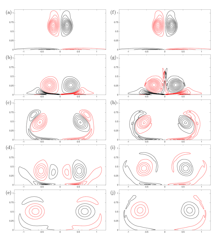
Figure 1: Time sequence of vorticity contours for a two-dimensional vortex pair interacting with a wall at $t=1$, $3$, $6$, $10$ and $15\delta^{2}/\Gamma_{0}$ for a Newtonian fluid ($a$-$e$) and a viscoelastic fluid ($f$-$j$). Contour levels are from -$15$ to $15$ with negative values indicated by red dashed lines.

Figure 2: Contours of $B_{xx}$ ($a$), $B_{xy}$ ($b$), $B_{yy}$ ($c$) and of the trace of the tensor ${\bf B}$, normalized with $L^{2}$ ($d$) at $t=15\delta^{2}/\Gamma_{0}$

3.2 Bubbly flow

Fluid-fluid interfaces are captured by the interface-correction level-set method ⁷³, and the surface tension force is described by the continuum surface force (CSF) model. The second-order Adams-Bashforth scheme (AB2) is used for the integration of governing equations of an EVP bubbly flow. Note that the AB2 scheme is used to facilitate the implementation of the fast pressure-correction method developed by Dong and Shen ⁸⁰ and Dodd and Ferrante ⁸¹.

3.2.1 Level-set method

In two-fluid systems, an interface between the phases can be resolved using a fully Eulerian method. The body force ${\bf f}$ due to surface tension, see Eqs. (1b), is expressed as:

$${\bf f}=\sigma\kappa\delta(\phi)\bf n,$$ (4)

where $\delta$ is a regularized delta function and $\sigma$ is the surface tension.

In this paper, we have adopted a mass-conserving, interface-correction level-set method to capture an interface by a continuous level-set function. The level-set function $\phi({\bf x},t)$ approximates the signed distance from the interface. Hence, $\phi=0$ denotes the interface, $\phi>0$ denotes fluid 1 and $\phi<0$ fluid 2. The interface is convected with the local velocity field, i.e.

$$\frac{\partial\phi}{\partial t}+{\bf u}\cdot\nabla\phi=0.$$ (5)

To calculate the body force in Eq. 4, the unit normal vector, ${\bf n}$, and the local mean curvature, $\kappa$, can be simply computed as

$${\bf n}=\frac{\nabla\phi}{|\nabla\phi|},$$ (6)

$$\kappa=-\nabla\cdot{\bf n}.$$ (7)

With time, if simply advected, the level set field will no longer equal a signed distance to the interface. It is essential that the signed distance property is preserved near the interface, because of the normal and curvature computation. We therefore redistance the level set field every 10-20 time steps by solving the Hamilton-Jacobi (reinitialization) equation:

$${\frac{\partial\phi}{\partial{\mathcal{T}}}+S(\phi_{0})(|\nabla\phi|-1)=0,}$$ (8)

where $\phi_{0}$ is the level set field before redistancing, ${\mathcal{T}}$ is pseudo-time and $S(\phi_{0})$ is the mollified sign function ⁷³. One can observe that if a steady state is reached, then the zero level set contour (interface location) is unaltered, while the level set field has returned to a signed distance function. In practice, this equation is iterated only for a few steps towards steady state. The level set advection Eq. (5) and reinitialization Eq. (8) are solved using a three-stage total-variation-diminishing (TVD) third-order Runge-Kutta scheme ⁸².

The density, the solvent and the polymeric viscosities, and the relaxation time vary across the fluid interface and are expressed in a mixture form as

$$\begin{split}\rho&=\rho_{1}H(\phi)+\rho_{2}\big{(}1-H(\phi)\big{)},\quad\lambda=\lambda_{1}H(\phi)+\lambda_{2}\big{(}1-H(\phi)\big{)},\\ \mu_{s}&=\mu_{s,1}H(\phi)+\mu_{s,2}\big{(}1-H(\phi)\big{)},\quad\mu_{p}=\mu_{p,1}H(\phi)+\mu_{p,2}\big{(}1-H(\phi)\big{)},\end{split}$$ (9)

where the subscripts $1$ and $2$ denote the properties of the bulk and suspended fluids, respectively, and $H(\phi)$ is the regularized Heaviside function defined such that it is zero inside the bubbles and unity outside.

A complete description of the level set methodology can be found in Sussman et al.⁸³ and Ge et al.⁷³, and references therein.

3.2.2 Time integration: Adams-Bashforth scheme

To advance the solution from time level $n$ to $n+1$, we proceed as follows. First, we advance the level set function and update the density and viscosity fields accordingly. Second, we advance the extra stress tensor and the velocity field in time with the second-order Adams-Bashforth scheme as

$${\bf B}^{n+1}={\bf B}^{n}+\Delta t\bigg{(}\frac{3}{2}{\bf RT_{ab}}^{n}-\frac{1}{2}{\bf RT_{ab}}^{n-1}\bigg{)},$$ (10)

$${\bf u}^{*}={\bf u}^{n}+\Delta t\bigg{(}\frac{3}{2}{\bf RU_{ab}}^{n}-\frac{1}{2}{\bf RU_{ab}}^{n-1}\bigg{)},$$ (11)

where we have defined the right-hand sides of the Eqs. (2) ${\bf RT_{ab}}^{n}$ and of eq. (1b) as ${\bf RU_{ab}}^{n}$, with

$${\bf RT_{ab}}^{n}=\bigg{[}\frac{1}{\lambda}\bigg{(}a{\bf I}-\mathcal{F}{\bf B}\bigg{)}-\bigg{(}{\bf u}\cdot\nabla{\bf B}-{\bf B}\cdot\nabla{\bf u}-\nabla{\bf u}^{T}\cdot{\bf B}\bigg{)}\bigg{]}^{n},$$ (12)

$${\bf RU_{ab}}^{n}= -\nabla\cdot({\bf u}{\bf u})^{n}+{\bf g}+\frac{1}{\rho^{n+1}}\bigg{(}\nabla\cdot\big{[}\mu_{s}^{n+1}(\nabla{\bf u}^{n}+(\nabla{\bf u}^{n})^{T})\big{]}+\nabla\cdot\bm{\tau}^{n}+\sigma\kappa^{n+1}\delta(\phi^{n+1}){\bf n}^{n+1}\bigg{)}.$$ (13)

To enforce a divergence-free velocity field, Eq. (1a), we proceed by solving the Poisson equation for the pressure ⁸⁴, i.e.

$$\nabla\cdot\bigg{(}\frac{1}{\rho^{n+1}}\nabla p^{n+1}\bigg{)}=\frac{1}{\Delta t}\nabla\cdot{\bf u}^{*},$$ (14)

and finally, the velocity at the next time level is corrected as

$${\bf u}^{n+1}={\bf u}^{*}-\frac{\Delta t}{\rho^{n+1}}\nabla p^{n+1}.$$ (15)

In the droplet-laden flow, the pressure Poisson equation is solved in both phases, with unequal densities. Per default, the left hand side of the Poisson equation has variable coefficients. In order to utilise an efficient FFT-based pressure solver with constant coefficients ⁷³, we use the following splitting of the pressure term ⁸⁰:

$${\frac{1}{\rho^{n+1}}\nabla p^{n+1}\to\frac{1}{\rho_{0}}\nabla p^{n+1}+\left(\frac{1}{\rho^{n+1}}-\frac{1}{\rho_{0}}\right)\nabla\left(2p^{n}-p^{n-1}\right),}$$ (16)

where $\rho_{0}$ is the density of the lower density phase (a constant). With this splitting, and after multiplying by $\rho_{0}$, the Poisson equation (Eq. 14) becomes:

$$\nabla\cdot\nabla p^{n+1}=\nabla\cdot\left[\left(1-\frac{\rho_{0}}{\rho^{n+1}}\right)\nabla\left(2p^{n}-p^{n-1}\right)\right]+\frac{\rho_{0}}{\Delta t}\nabla\cdot{\bf u}^{*}.$$ (17)

and the velocity correction (Eq. 15) transforms to:

$${\bf u}^{n+1}={\bf u}^{*}-\Delta t\left[\frac{1}{\rho_{0}}\nabla p^{n+1}+\left(\frac{1}{\rho^{k}}-\frac{1}{\rho_{0}}\right)\nabla\left(2p^{n}-p^{n-1}\right)\right].$$ (18)

3.3 Particle-laden flow

The governing equations of EVP particle-laden flow are integrated in time with a third order Runge-Kutta (RK3) scheme. The RK3 scheme is third order accurate, low storage, and improves the numerical stability of the code, allowing for larger time steps. Both rigid and deformable particles are considered here. The rigid particles are included using the immersed boundary method (IBM) that allows us to solve the Navier-Stokes equations on a Cartesian grid despite the presence of particles or complex wall geometries, and has become a popular tool in recent years. The IBM consists of an extra force, added to the right-hand side of the momentum equations, see Eqs. (1b), to mimic boundary conditions, creating virtual boundaries inside the numerical domain. This extra force acts in the vicinity of a solid surface to impose indirectly the no-slip/no-penetration (ns/np) boundary condition.

In the case of deformable particles, we use the method described in Rosti and Brandt ^{74, 85, 86}. The solid is an incompressible viscous hyper-elastic material undergoing only the isochoric motion, where the hyper-elastic contribution is modeled as a neo-Hookean material, thus satisfying the incompressible Mooney-Rivlin law. To numerically solve the fluid-structure interaction problem, we adopt the so called one-continuum formulation ⁸⁷, where only one set of equations is solved over the whole domain. Thus, at each point of the domain the fluid and solid phases are distinguished by the local solid volume fraction $\phi_{s}$, which is equal to $0$ in the fluid, $1$ in the solid, and between $0$ and $1$ in the interface cells. The set of equations can be closed in a purely Eulerian manner by introducing a transport equation for the volume fraction $\phi_{s}$ (the equation is formally the same used in the level-set method, i.e., equation (5)). The instantaneous local value of the elastic force is found by solving equation (2), which represents the upper convected derivative of the left Cauchy-Green deformation tensor. The right hand side of equation (2) is identically zero for a hyperelastic material ⁸⁸.

3.3.1 Time integration: Runge-Kutta scheme

When using the third order Runge-Kutta scheme, the extra stress tensor and the unprojected field are computed by defining ${\bf RT_{rk3}}^{k}$ and ${\bf RU_{rk3}}^{k}$ as

$${\bf RT_{rk3}}^{k}= \zeta^{k}\bigg{[}\frac{1}{\lambda}\bigg{(}a{\bf I}-\mathcal{F}{\bf B}\bigg{)}-\bigg{(}{\bf u}\cdot\nabla{\bf B}-{\bf B}\cdot\nabla{\bf u}-\nabla{\bf u}^{T}\cdot{\bf B}\bigg{)}\bigg{]}^{k-1}$$ (19)

$$+ \xi^{k}\bigg{[}\frac{1}{\lambda}\bigg{(}a{\bf I}-\mathcal{F}{\bf B}\bigg{)}-\bigg{(}{\bf u}\cdot\nabla{\bf B}-{\bf B}\cdot\nabla{\bf u}-\nabla{\bf u}^{T}\cdot{\bf B}\bigg{)}\bigg{]}^{k-2},$$

$$\begin{split}{\bf RU_{rk3}}^{k}=&-\zeta^{k}\nabla\cdot({\bf u}{\bf u})^{k-1}-\xi^{k}\nabla\cdot({\bf u}{\bf u})^{k-2}-2\frac{\alpha^{k}}{\rho}\nabla p^{k-1}+\frac{\alpha^{k}}{\rho}\bigg{(}\nabla\cdot\big{[}\mu_{s}(\nabla{\bf u}+(\nabla{\bf u})^{T})\big{]}+\nabla\cdot\bm{\tau}\bigg{)}^{k}\\ &+\frac{\alpha^{k}}{\rho}\bigg{(}\nabla\cdot\big{[}\mu_{s}(\nabla{\bf u}+(\nabla{\bf u})^{T})\big{]}+\nabla\cdot\bm{\tau}\bigg{)}^{k-1},\end{split}$$ (20)

which are the right-hand sides of the Eqs. (2) and (1b). Integrating in time yields

$${\bf B}^{k}={\bf B}^{k-1}+\Delta t{\bf RT_{rk3}}^{k},$$ (21)

$${\bf u}^{*}={\bf u}^{k-1}+\Delta t{\bf RU_{rk3}}^{k}.$$ (22)

In the previous equations, $\Delta t$ is the overall time step from $t^{n}$ to $t^{n+1}$, the superscript ^∗ is used for the predicted velocity, while the superscript ^k denotes the Runge-Kutta substep, with $k=0$ and $k=3$ corresponding to times $n$ and $n+1$.

The pressure equation that enforces the solenoidal condition on the velocity field is solved via a Fast Poisson Solver

$$\nabla\cdot\nabla\psi^{k}=\frac{\rho}{2\alpha^{k}\Delta t}\nabla\cdot{\bf u}^{*},$$ (23)

and, finally, the pressure and velocity are corrected according to

$$p^{k} =p^{k-1}+\psi^{k},$$ (24a)

$${\bf u}^{k} ={\bf u}^{*}-2\alpha^{k}\frac{\Delta t}{\rho}\nabla\psi^{k},$$ (24b)

where $\psi$ is the projection variable, and $\alpha$, $\zeta$, and $\xi$ are the integration constants, whose values are

$$\begin{array}[]{ccc}\alpha^{1}=\frac{4}{15}&\alpha^{2}=\frac{1}{15}&\alpha^{3}=\frac{1}{6}\\ \\ \zeta^{1}=\frac{8}{15}&\zeta^{2}=\frac{5}{12}&\zeta^{3}=\frac{3}{4}\\ \\ \xi^{1}=0&\xi^{2}=-\frac{17}{60}&\xi^{3}=-\frac{5}{12}.\end{array}$$ (25)

3.3.2 Immersed boundary method

The IBM force f cannot be formulated by means of a universal equation and therefore IBMs differ in the way f is computed. The method applied in this solver was first developed by Peskin ⁶⁸ and numerous modifications and improvements have been suggested since (for a review, see Ref. ⁸⁹). In this study we use two different IBM schemes: the volume penalization IBM ^{90, 91} to generate obstacles and complex geometries, and the discrete forcing method for moving particles ^{92, 70, 72} to fully resolve particle suspensions in elastoviscoplastic flows.

Volume penalization IBM

Kajishima et al.and Breugem et al.^{90, 91} proposed the volume penalization IBM, where the IBM force f is calculated from the first prediction velocity $\textbf{u}^{*}$ that is obtained by integrating Eq. (1b) in time without considering the IBM force and the pressure correction. The IBM force f and the second prediction velocity $\textbf{u}^{**}$ are then calculated as follows:

$$\textbf{f}_{ijk}\,= \,\rho\,\alpha_{ijk}\frac{{\left(\textbf{u}_{s}-\textbf{u}^{*}\right)}_{ijk}}{\Delta t}\,,$$ (26a)

$$\textbf{u}^{**}_{ijk}\,= \,\textbf{u}^{*}_{ijk}\,+\,\Delta t\,\textbf{f}_{ijk}/\rho\,,$$ (26b)

where $\alpha_{ijk}$ is the solid volume fraction in the grid cell with index $(i,j,k)$, varying between $0$ (entirely located in the fluid phase) and $1$ (entirely located in the solid area) and $\textbf{u}_{s}$ is the solid interface velocity within this grid cell. Figure 3 indicates the solid volume fractions (highlighted area) for grid cells around $u(i,j)$ and $v(i-1,j-1)$. Solid boundary in this figure is shown by red dashed line. For non-moving boundaries, $\textbf{u}_{s}$ is $0$ and Eq. 26 reduce to:

$$\textbf{u}^{**}_{ijk}=\left(1-\alpha_{ijk}\right)\textbf{u}^{*}_{ijk}\,.$$ (27)

The second prediction velocity $\textbf{u}^{**}$ is then used to update the velocities and the pressure following a classical pressure correction scheme ⁹².

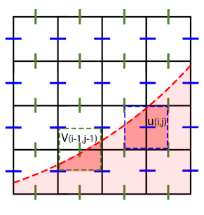
Figure 3: Solid volume fractions (highlighted area) for grid cells around $u(i,j)$ and $v(i-1,j-1)$. Solid boundary is shown by red dashed line.

The volume penalization IBM is computationally very efficient, since the solid volume fractions around the velocity points can be calculated at the beginning of the simulation using an accurate method, or they can even be extracted directly from a physical sample by magnetic resonance imaging or X-ray computed tomography ⁹¹.

Discrete forcing method for moving particles

Following the IBM framework, we impose the no-slip/no penetration condition at the particle surfaces (Figure 4) by adding an extra force f on the right hand side of the fluid momentum equations (1b). Uhlmann ⁹³ developed a computationally efficient IBM to fully resolve particle-laden flows. Breugem ⁹² introduced improvements to this method, making it second order accurate in space by applying a multi-direct forcing scheme ⁹⁴ to better approximate the no-slip/no-penetration (ns/np) boundary condition on the surface of the particles and by introducing a slight retraction of the grid points on the surface towards the interior. The numerical stability of this method for particle over fluid density ratio near unity was also improved by accounting the inertia of the fluid contained within the particles ⁹⁵. Ardekani et al.⁷² extended the original method to simulate suspension of spheroidal particles with lubrication and contact models for the short-range particle-particle (particle-wall) interactions.

Figure 4: Uniform distribution of Lagrangian points over the surface of an spheroidal particle with an aspect ratio (polar over equatorial radius) $1/3$.

In this study, we apply the same scheme to fully resolved simulations of particle suspensions in elastoviscoplastic flows. We apply the IBM force on the predicted velocities $\textbf{u}^{*}$, which have been obtained as in the single-phase situation. The second prediction velocity $\textbf{u}^{**}$ is then obtained after the application of the IBM force, and $\textbf{u}^{**}$ substitutes $\textbf{u}^{*}$ in the pressure correction scheme given in the previous section. The formulation to calculate the second prediction velocity is given here:

$$\textbf{U}^{*}_{l}=\sum\limits_{ijk}\textbf{u}^{*}_{ijk}\delta_{d}\left(\textbf{x}_{ijk}-\textbf{X}^{k-1}_{l}\right)\Delta x\Delta y\Delta z\,,$$ (28a)

$$\textbf{F}^{k-1/2}_{l}=\rho_{f}\,\frac{\textbf{U}\left(\textbf{X}^{k-1}_{l}\right)-\textbf{U}^{*}_{l}}{\Delta t}\,,$$ (28b)

$$\textbf{f}^{\,k-1/2}_{\,ijk}=\sum\limits_{l}\textbf{F}^{k-1/2}_{l}\delta_{d}\left(\textbf{x}_{ijk}-\textbf{X}^{k-1}_{l}\right)\Delta V_{l}\,,$$ (28c)

$$\textbf{u}^{**}=\textbf{u}^{*}+\Delta t\,\textbf{f}^{\,k-1/2}/\rho_{f}\,,$$ (28d)

where capital letters indicate the variable at a Lagrangian point with index $l$. In equation (28a), we interpolate the first prediction velocity $\textbf{u}^{*}$ from the Eulerian grid to the Lagrangian points on the surface of the particle, $\textbf{U}^{*}_{l}$, using the regularized Dirac delta function $\delta_{d}$ of Roma et al.⁹⁶. This approximated delta function essentially replaces the sharp interface with a thin porous shell of width $3\Delta x$; it preserves the total force and torque on the particle in the interpolation, provided that the Eulerian grid is uniform. The IBM force at each Lagrangian point, $\textbf{F}^{k-1/2}_{l}$, is proportional to the difference between the interpolated predicted velocity and the local velocity of the surface of the particle (for rigid particles, $\textbf{U}_{p}+\boldsymbol{\omega}_{p}\times\textbf{r}$, calculated as shown in the paragraph below). In equation (28c), the IBM forces obtained at the Lagrangian points are interpolated back to the Eulerian grid by the same regularized Dirac delta function. In equation (28d), the IBM forces in the Eulerian grid ($\textbf{f}^{\,k-1/2}_{\,ijk}$) are added to the first prediction velocity to obtain the second prediction velocity $\textbf{u}^{**}$.

Given the smooth delta function and resolutions typically used, the Eulerian forces obtained from two neighboring Lagrangian points overlap. The multidirect forcing scheme proposed by Luo et al.⁹⁴ is therefore employed to iteratively determine the IBM forces such that the no-slip boundary conditions, $\textbf{U}^{**}\approx\textbf{U}$, are collectively imposed at the Lagrangian grid points. The new second prediction velocity $\textbf{u}^{**}$ is then obtained by solving the equations above iteratively (typically 3 iterations is enough) using the new $\textbf{u}^{**}$ as $\textbf{u}^{*}$ at the beginning of the next iteration with equation 28b substituted by:

$$\textbf{F}^{k-1/2}_{l}=\textbf{F}^{k-1/2}_{l}+\rho_{f}\,\frac{\textbf{U}\left(\textbf{X}^{k-1}_{l}\right)-\textbf{U}^{**}_{l}}{\Delta t}\,.$$ (29)

The second prediction velocity $\textbf{u}^{**}$ is then used to update the velocities and the pressure following the procedure described in the previous section.

Taking into account the inertia of the fictitious fluid phase inside the particle volumes, Breugem ⁹² showed that equations for particle motion can be rewritten as:

$$\rho_{p}V_{p}\frac{\mathrm{d}\textbf{U}_{p}}{\mathrm{d}t} \approx -\sum\limits_{l=1}^{N_{L}}\textbf{F}_{l}\Delta V_{l}+\rho_{f}\frac{\mathrm{d}}{\mathrm{d}t}\left(\int_{V_{p}}\textbf{u}\mathrm{d}V\right)+\left(\rho_{p}-\rho_{f}\right)V_{p}\textbf{g}+\textbf{F}_{c},\,$$ (30)

$$\frac{\mathrm{d}\left(\textbf{I}_{p}\,\boldsymbol{\omega}_{p}\right)}{\mathrm{d}t} \approx -\sum\limits_{l=1}^{N_{L}}\left(\textbf{r}_{l}\times\textbf{F}_{l}\right)\Delta V_{l}+\rho_{f}\frac{\mathrm{d}}{\mathrm{d}t}\left(\int_{V_{p}}\left(\textbf{r}\times\textbf{u}\right)\mathrm{d}V\right)+\textbf{T}_{c}\,.$$ (31)

where $\textbf{U}_{p}$ and $\boldsymbol{\omega}_{p}$ are the particle translational and the angular velocity, $\rho_{p}$, $V_{p}$ and $\textbf{I}_{p}$ are the mass density, volume and moment-of-inertia tensor of a particle, and r is the position vector with respect to the center of the particle. The first terms on the right hand side of these equations are the summation of IBM forces and torques that act on each Lagrangian point. The second terms account for the translational and angular acceleration of the fluid trapped inside the particle shell. The force term $-\rho_{f}V_{p}\textbf{g}$ accounts for the hydrostatic pressure with g the gravitational acceleration, and $\textbf{F}_{c}$ and $\textbf{T}_{c}$ are the force and torque resulting from particle-particle (particle-wall) collisions (see ⁷² for more details). These equations are integrated in time using the Runge-Kutta scheme, as explained in the previous section.

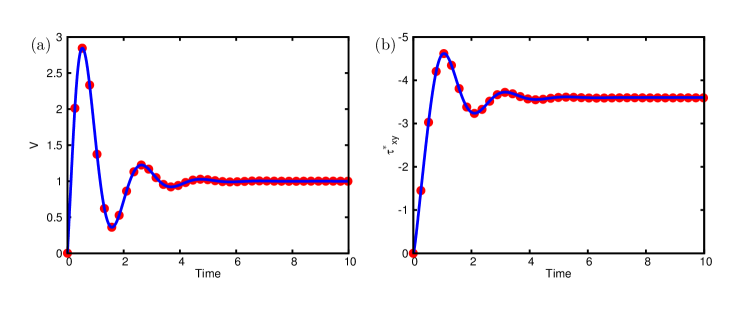
Figure 5: Start-up Poiseuille flow for an Oldroyd-B fluid. (a) Time evolution of the centerline streamwise velocity component and (b) $\tau^{*}_{xy}$ stress at channel wall. The symbols represent our numerical results while the solid lines are the analytical solution derived by Waters and King ⁹⁷. ($Re=0.125$, $Wi=0.125$ and $\beta=0.1$).

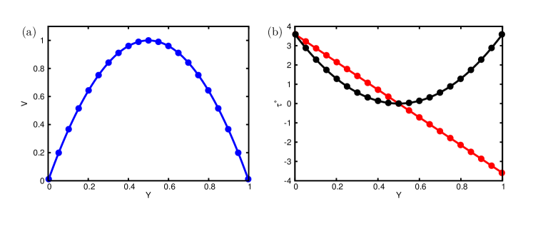
Figure 6: Poiseuille flow of an Oldroyd-B fluid. (a) Steady state streamwise velocity component profile, (b) $\tau^{*}_{xx}$ (black color) and $\tau^{*}_{xy}$ (red color) stress profiles. The symbols represent our numerical results while the solid lines are the analytical solution derived by Waters and King ⁹⁷. ($Re=0.125$, $Wi=0.125$ and $\beta=0.1$).

Figure 7: Poiseuille flow of a FENE-P fluid. (a) Steady state streamwise velocity component profile, (b) $B_{xx}$ (black color) and $B_{xy}$ (red color) profiles. The symbols represent our numerical results while the solid lines are the analytical solution. ($Re=300$, $Wi=25$ and $\beta=0.9$).

4 Validation

4.1 Single-phase flow

4.1.1 Poiseuille flow of a viscoelastic fluid

The first test case deals with the start-up Poiseuille flow of an Oldroyd-B and FENE-P fluid ($Bi=0$) in a planar channel. The geometry is a two-dimensional channel bounded by two parallel walls separated by a distance $h=L_{y}$, where $y$ denotes the wall-normal direction, and $x$ is the streamwise direction. The fluid is initially at rest and set into motion by applying a sudden constant pressure gradient in the streamwise direction. No-slip boundary conditions are applied at the walls. As our method solves the three-dimensional Navier-Stokes equations, we impose periodic boundary conditions in the streamwise and spanwise directions to emulate the two-dimensional geometry. The following dimensionless variables are introduced:

$$Y=\frac{y}{h};\,\tau^{*}=\frac{\tau h}{u_{0}(\mu_{s}+\mu_{p})};\,T=\frac{t(\mu_{s}+\mu_{p})}{\rho h^{2}};\,V=\frac{u}{u_{0}};\,\beta=\frac{\mu_{s}}{\mu_{s}+\mu_{p}};\,Re=\frac{\rho u_{0}h}{\mu_{s}+\mu_{p}};\,Wi=\frac{\lambda u_{0}}{h},$$ (32)

where $\tau^{*}$ is a non-dimensional stress, $T$ is a non-dimensional time and the velocity scale is $u_{0}=-h^{2}dp/dx/8(\mu_{s}+\mu_{p})$. The uniform grid has the grid size $\Delta y=h/180$. The time-evolution of the centerline velocity and the wall shear stress is shown for the Oldroyd-B fluid case in Fig. 5. The velocity and the stress components show oscillating behaviour with overshoots and undershoots before settling down to their fully developed values. The steady state profiles for velocity and stress components are shown in Figs. 6 and 7 for the Oldroyd-B and FENE-P fluids, respectively. As can be seen from these figures, there is an excellent agreement between our numerical and existing analytical results.

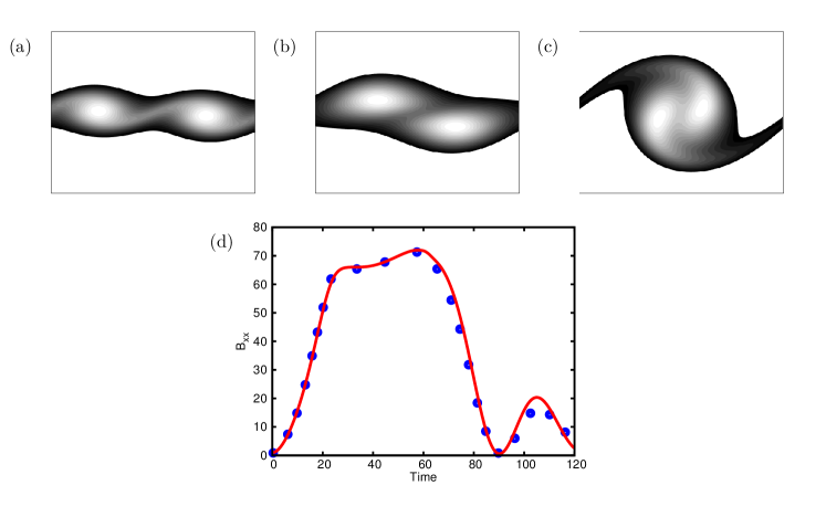
Figure 8: (a-c) Instantaneous contours of the absolute value of vorticity at time $T\approx 20$, $60$ and $100$. The color scale from black to white ranges from $0.05$ to $0.4$ in (a), from $0.05$ to $0.3$ in (b) and from $0.05$ to $0.25$ in (c). (d) Time evolution of the $B_{xx}$ component of the polymer conformation tensor. The red line displays our numerical results, while the symbols display the results of Min et al.⁷⁷. ($Re=50,Wi=25,\beta=0.9,L^{2}=100$).

4.1.2 Temporally evolving mixing layer of a viscoelastic fluid

The FENE-P model implementation has been validated by simulating a viscoelastic temporally evolving mixing layer flow and by comparing our results with those provided by Min et al.⁷⁷. We consider the initial velocity field $u=0.5(\tanh y)$, and trigger the roll-up of the shear layer with a small $2D$ perturbation. The characteristic velocity and length scales are $\Delta u=u_{\textrm{max}}-u_{\textrm{min}}$ and $\delta=\Delta u/(du/dy)_{\textrm{max}}$, respectively. The Reynolds number is fixed at $Re=\rho\delta\Delta u/\mu_{s}=50$ and the Weissenberg number at $Wi=\lambda\Delta u/\delta=25$; moreover, the extensibility $L^{2}$ is set to $100$, and the solvent viscosity ratio tp $\beta=0.9$. The dimensionless time is defined as $T=t\Delta u/\delta$. The $2D$ numerical domain has the size $30\delta\times 100\delta$, discretised by $128\times 384$ grid points. Note that the flow configuration and domain are the same used by Min et al.⁷⁷. Figures 8(a - c) show the instantaneous vorticity contours for the Newtonian flow, where we can observe that the initial perturbation grows in time and generates two vortices (panel a - $T\approx 20$), which subsequently roll up (panel b - $T\approx 60$) and eventually merge into one large vortex (panel c - $T\approx 100$); the polymeric flow shows a similar behavior. The quantitative validation is shown in the bottom panel, where we plot the time history of $B_{xx}$ in the center of the domain: the symbols represent the literature results, whereas the red line indicates our numerical data. We find a good agreement of the conformation tensor component time history over the whole vortex merging process.

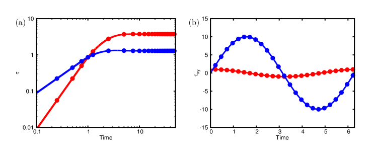
Figure 9: Simple and oscillating shear flow. (a) The evolution of $\tau_{xx}$ (red) and $\tau_{xy}$ (blue) for simple shear flow. (b) The evolution of the shear EVP stress for an oscillating shear flow at $Bi=0$ (red) and $300$ (blue). The solid lines represent the analytical solution by Saramito ⁸ while the symbols are our numerical results. (Simple shear flow: $Bi=1$, $Wi=1$ and $\beta=1/9$. Oscillating shear flow: $Wi=0.1$ and $\beta=0$).

4.1.3 Shear flow of an elastoviscoplastic fluid

Next, the method is validated for elastoviscoplastic (EVP) single-phase flows. For this purpose, two test cases are considered. The first case is a simple shear flow. Initially, the fluid is at rest and set into motion by a constant shear rate $\dot{\gamma}_{0}$. This test case has a constant dimensionless velocity gradient $\nabla{\bf u}=\bigl{[}\begin{smallmatrix}0&1\\ 0&0\end{smallmatrix}\bigr{]}$, the Weissenberg number $Wi=\lambda\dot{\gamma}_{0}=1$, the Bingham number $Bi=\tau_{0}/\mu_{0}\dot{\gamma}_{0}=1$, and the viscosity ratio $\beta=1/9$. The time evolution of the stresses is shown in Fig. 9(a). The stress components increase as long as the yield criterion is not satisfied; once the criterion is fulfilled (T $\approx$ 1), the energy starts to dissipate as a result of viscous effects, which is clearly seen in the figure as the slope of the time evolution of the stresses decreases significantly.

The second test case considers the periodic shear flow of an EVP fluid. An oscillatory flow is applied by imposing the shear strain $\gamma_{0}sin(\omega t)$, where $\gamma_{0}$ is the strain amplitude and $\omega$ is the angular frequency of the oscillation. The Weissenberg number is defined as $Wi=\lambda\omega$ and the Bingham number as $Bi=\tau_{y}/(\rho\gamma_{0}\omega)$ in this case. Computations are performed for two different Bingham numbers, i.e., $Bi=0$ and $300$. Note that these two values are extreme cases for which the material behaves like a viscoelastic fluid ($Bi=0$) and like an elastic solid ($Bi=300$). The viscoelastic case can be reached at large strain amplitudes $\gamma_{0}\rightarrow\infty$, whereas the elastic solid behavior is obtained when the amplitude is small $\gamma_{0}\rightarrow 0$. The other dimensionless parameters of the problem are kept constant at $Wi=0.1$ and $\beta=0$. The evolution of the shear stress component $\tau_{xy}$ is displayed in Fig. 9(b) for $Bi=0$ and $300$. As can be seen in these figures, there is a good agreement between our simulation and the analytical solutions, thus indicating an accurate solution of the EVP model equations.

4.2 Multiphase flow in complex fluids

Table 2: Comparison of the settling velocity of a sphere in EVP fluid.

	$V$ (mm s-1)
Present work	0.356
Fraggedakis et al.23	0.364
Holenberg et al.24	0.37

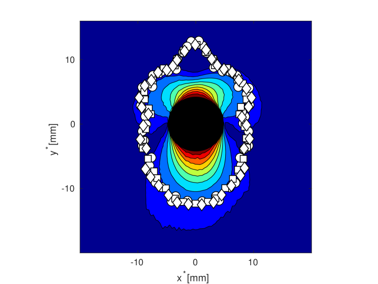
Figure 10: Sphere settling in EVP fluid. Velocity magnitude, scaled with the terminal velocity of the settling sphere. The different symbols represent different experimental series for the solid-fluid boundary defined by Holenberg et al.²⁴. ($Ar=0.03$, $Wi=1.04$, $Bn=0.089$, $\rho^{\circ}=1.38$ and $\beta=0.01$).

4.2.1 Sedimentation of a spherical particle in an elastoviscoplastic fluid

After validating the numerical method for simple viscometric flows, the method is now applied to study the sedimentation of a spherical particle in a channel filled with an EVP fluid. This problem exhibits different viscometric flows simultaneously, i.e., biaxial stretching upstream of the particle, shear flow on the sides, and uniaxial extensional flow downstream of it. The Saramito model is employed here to facilitate comparison of the present results with the numerical results by Fraggedakis et al.²³ and with the experimental data by Holenberg et al.²⁴. A single spherical particle of radius $R$ is centered in a domain of size $(L_{x}\times L_{y}\times L_{z})=(12R\times 20R\times 12R)$; a grid of $144\times 240\times 144$ points is used to discretize the computational domain. Periodic boundary conditions are imposed in the $x$ (spanwise) and $y$ (gravity) directions whereas a free slip/no penetration condition is enforced in the $z$ direction. The particle starts moving due to the gravity in an otherwise quiescent ambient EVP fluid. Following Fraggedakis et al.²³, the non-dimensional parameters are defined as follows:

$$Ar=\frac{\Delta\rho^{2}gR^{3}}{\mu_{s}+\mu_{p}};\quad Wi=\frac{\lambda\Delta\rho gR}{\mu_{s}+\mu_{p}};\quad Bn=\frac{\tau_{y}}{\Delta\rho gR};\quad\rho^{\circ}=\frac{\rho_{s}}{\rho_{f}},$$ (33)

where $Ar$, $Wi$, $Bn$, and $\rho^{\circ}$ represent the Archimedes number, the Weissenberg number, the Bingham number, and the density ratio, respectively. In Eq. (33), the density difference is defined as $\Delta\rho=\rho_{f}(\rho^{\circ}-1)=\rho_{s}-\rho_{f}$, where $\rho_{s}$ and $\rho_{f}$ are the solid and the fluid densities, respectively. The present results are compared with the computational simulations by Fraggedakis et al.²³ and the experimental results by Holenberg et al.²⁴. The simulation is performed for $Ar=0.03$, $Wi=1.04$, $Bn=0.089$, $\rho^{\circ}=1.38$ and $\beta=0.01$. Note that the “rough heavy sphere" case is considered in the present study, referring to the no-slip boundary condition on the particle. First, a quantitative comparison is conducted based on the steady state settling speed of the particle in the EVP fluid. The terminal velocity predicted by the present study, the one in the numerical simulation in Ref. ²³ and the one observed experimentally ²⁴ are reported in Table 2. As can be seen from the table, the present results could capture the terminal velocity accurately, and indeed the result of the present study deviates from that in other published studies by less than $4\%$. Next, we present a qualitative comparison of the velocity fields around the spherical particle. The steady state velocity contours normalized with the particle terminal velocity are displayed in Fig. 10. Direct comparisons with the experimental data of ²⁴ are also included for the yield surface represented by the white markers around the sphere, where the circular and square marks indicate two different experimental series. Holenberg et al.²⁴ determined the yielded region by means of PIV and PTV techniques, i.e., they defined the yielded region where the velocity magnitude exceeded $10\%$ of the settling velocity. To facilitate direct comparison with experimental data, the velocity contours shown in Fig. 10 are constructed as follows: the distance between the consecutive contour lines is the same and equals to $10\%$ of the terminal velocity, starting from $10\%$ to $90\%$ of the velocity. Generally, we are in good agreement with the experimental marks ²⁴ and simulation results shown in Fig. 9 in the work of Fraggedakis et al. ²³. Similarly to ²³, the current methodology could capture the expected loss of the fore-aft symmetry. On the other hand, a slight discrepancy between the present results and those by the aforementioned work ²³ can be attributed to a different computational box and a lower resolution. Indeed, in the present study a full three-dimensional flow is employed, whereas Fraggedakis et al.²³ consider an axisymmetric configuration. Moreover, local grid refinement is used in Ref. ²³. Their very fine grid in the vicinity of the sphere may result in an improved resolution of the yielded region. Another reason could be the employment of different boundary conditions in the far-field boundary, the open-boundary condition is used by Fraggedakis et al.²³ while a periodic boundary condition is employed in the present work.

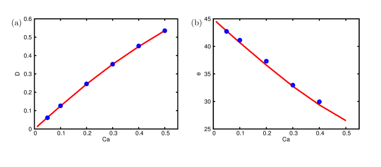
Figure 11: Steady deformation of a neo-Hookean elastic particle in a Newtonian fluid for $0.05\leq Ca\leq 0.5$. (a) Taylor parameter $D$ and (b) inclination angle $\theta$ vs. $Ca$. Red line: numerical results from Ref. ⁴⁷; blue circles: our numerical simulation. ($Re=0.1$).

4.2.2 Deformable dilute suspension in a shear flow

Steady deformation of a neo-Hookean elastic particle in a shear flow

In this test case, we simulate the flow in a plane Couette geometry. We use a Cartesian uniform mesh in a rectangular box of size $16R\times 10R\times 16R$, with 16 grid points per particle radius $R$. Periodic boundary conditions are imposed in the streamwise ($x$) and spanwise ($z$) directions, and the no-slip condition at the walls ($y=-h$ and $y=h$), which move in two opposite directions with a constant streamwise velocity $\pm U=h\dot{\gamma}$. The Reynolds number $Re=\rho\dot{\gamma}R^{2}/\mu$ is fixed at $0.1$ and the Capillary number $Ca=\mu\dot{\gamma}/G$ varied one order of magnitude between $0.05$ and $0.5$. After the transients die out, the sphere deforms to approximately an ellipsoid, and we therefore characterize these shapes by the Taylor parameter ($D$) and the angle $\theta$. The Taylor deformation parameter is defined as $D=(L-B)/(L+B)$, where $L$ and $B$ are the major and minor axis of the equivalent ellipsoid in the middle plane, and $\theta$ is the inclination angle with the respect to the streamwise direction. The steady state values of $D$ and $\theta$ are reported in Fig. 11 for different $Ca$, and compared with those by Villone et al.⁴⁷. Similarly to the case of a viscoelastic droplet in a Newtonian medium, deformation as well as the tendency to align with the flow increases with $Ca$, i.e. with the deformability. A very good agreement is found between our numerical results and those in the literature. Further validation and details of our implementation can be found in ^{74, 85, 86}.

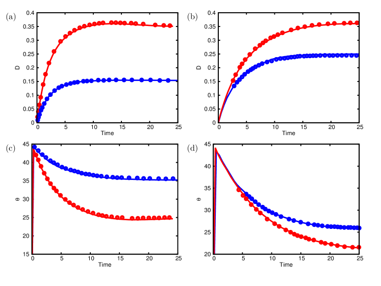
Figure 12: Drop deformation under simple shear flow for viscoelastic droplet in Newtonian medium (VN) and for a Newtonian droplet in a viscoelastic medium (NV). The solid lines represent our results while the symbols are those in Ref. ⁹⁸ and ⁹⁹ for the VN (a and c) and NV (b and d) systems, respectively. Panels (a) and (b) show the temporal evolution of the deformation $D$, and the (c) and (d) the history of the angle $\theta$. For the VN case, $Ca=0.14$ (blue) and $0.32$ (red) and for the NV case, $\chi=0.46$ (blue) and $\chi=0.76$ (red). (VN case: $Re=0.05,De_{2}=1.54,\beta=0.68,k_{\rho}=1,k_{\mu}=1.5$ and $\chi=0.25$; NV case: $Re=0.1,De_{1}=1,Ca=0.2,\beta=0.68,k_{\rho}=1$ and $k_{\mu}=1.5$).

Three-dimensional viscoelastic droplet

Verhulst et al.⁹⁸ and Cardinaels et al.⁹⁹ considered fully three-dimensional shear-driven droplets in which either the droplet or the surrounding fluid is viscoelastic. The Oldroyd-B model is employed in the present study to facilitate a direct comparison with the results of Verhulst et al.⁹⁸ and Cardinaels et al.⁹⁹. The spherical droplet of radius $R$ is at the center of the computational domain. Opposite velocities, $V$ and $-V$, are enforced on the two walls located at $z=0$ and $z=H$ to obtain the shear rate $\dot{\gamma}=2V/H$. Periodic boundary conditions are imposed in the $x$ (spanwise) and $y$ (streamwise) directions and no-slip conditions at the two walls. Following Verhulst et al.⁹⁸ and Cardinaels et al.⁹⁹, the non-dimensional parameters are defined as follows: the Reynolds number $Re=\rho_{1}\dot{\gamma}R^{2}/\mu_{1}$, the capillary number $Ca=R\dot{\gamma}\mu_{1}/\sigma$, the Weissenberg number $Wi=\lambda\dot{\gamma}$, the viscosity ratio $k_{\mu}=\mu_{2}/\mu_{1}$, the density ratio $k_{\rho}=\rho_{2}/\rho_{1}$, and the confinement ratio $\chi=2R/H$. Alternatively, two Deborah numbers can be defined as $De_{1}=(1-\beta)Wi/Ca$ and $De_{2}=(1-\beta)Wi/(k_{\mu}Ca)$. The results are presented in terms of the Deborah number and dimensionless capilary time $t\dot{\gamma}/Ca$. The droplet deformation in the $y-z$ plane is measured by the Taylor deformation parameter introduced above. Following Ramanujan and Pozrikidis ¹⁰⁰, the inertia tensor of the drop is used to find the equivalent ellipsoid.

First, we consider the startup dynamics of an Oldroyd-B droplet in a Newtonian medium (VN). The viscoelastic spherical droplet is centred in a computational domain of size $L_{x}=H,L_{y}=2H,L_{z}=H$, which is discretised with a resolution of $\Delta x=\Delta y=\Delta z=H/192$. The simulations are performed at $Re=0.05,De_{2}=1.54,\beta=0.68,k_{\rho}=1,k_{\mu}=1.5$ and $\chi=0.25$. The time evolutions of the Taylor parameter and the angle of inclination for a viscoelastic droplet in a Newtonian fluid at $Ca=0.14$ and $0.32$ are depicted in Fig. 12(a) together with the numerical results by Verhulst et al.⁹⁸. As expected, the drop deformation and alignment with the flow increase with $Ca$. Also, the time evolution of both the Taylor parameter and the inclination angle are in good agreement with the results reported in Ref. ⁹⁸.

Next, the dynamics of a Newtonian droplet in an Oldroyd-B fluid (NV) is studied. The resolution is fixed at $\Delta x=\Delta y=\Delta z=H/64$ and the computational domain is $L_{x}=2H,L_{y}=4H,L_{z}=H$. The computations were performed for $Re=0.1,De_{1}=1,Ca=0.2,\beta=0.68,k_{\rho}=1$ and $k_{\mu}=1.5$. The time evolution of the drop deformation parameter and its orientation angle are shown in Fig. 12(b) for two different confinement ratios: $\chi=0.46$ and $\chi=0.76$. As can be seen in the figure, the confinement ratio increases both the drop deformation and the drop orientation angle. The comparison between the present results and those by Cardinaels et al.⁹⁹ shows good agreement.

4.2.3 Buoyancy-driven droplet in viscoelastic and elastoviscoplastic media

Finally, the method is validated for buoyancy-driven (rising) droplets. We start from a Newtonian droplet rising in a Newtonian and viscoelastic fluid. The Oldroyd-B model is used in the present work to facilitate direct comparison with the results by Prieto ¹⁰¹, Zainali et al.¹⁰² and Vahabi and Sadeghy ¹⁰³. The fully Newtonian case is a classical benchmark, see e.g., Hysing et al.¹⁰⁴. The domain is rectangular with the width $L_{x}=1$ and the height $L_{y}=2$. A spherical droplet with a radius $R$ is initially placed at the centerline of the channel at a distance of $L_{y}/4$ from the lower part of the channel. The no-slip boundary conditions are applied at the horizontal walls. It should be noted that Prieto ¹⁰¹ used the free-slip boundary conditions on the vertical walls, whereas Zainali et al.¹⁰² and Vahabi and Sadeghy ¹⁰³ imposed no-slip boundary conditions. The non-dimensional parameters pertaining to this problem are defined as: the Reynolds number $Re=\rho_{1}U_{g}L/\mu_{1}$, the E${\rm\ddot{o}}$tv${\rm\ddot{o}}$s number $Eo=\rho_{1}U_{g}^{2}L/\sigma$, the Weissenberg number $Wi=\lambda U_{g}/L$, Bingham number $Bi=\tau_{y}/\rho gL$, the viscosity ratio $k_{\mu}=\mu_{2}/\mu_{1}$, the density ratio $k_{\rho}=\rho_{2}/\rho_{1}$ and the confinement ratio $\chi=2R/L_{x}$. The reference length scale is $L=2R$, the velocity scale is $U_{g}=\sqrt{gL}$, where $g$ is the gravitational constant, and the time scale is $L/U_{g}$.

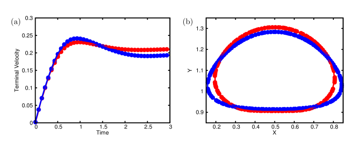
Figure 13: Buoyancy-driven viscoelastic two-phase system: Newtonian case (blue color) and Newtonian droplet in viscoelastic medium (red color). (a) The terminal velocity versus the non-dimensional time and (b) its respective steady state shape. The symbols represent the present results while the solid lines those by Prieto ¹⁰¹. Our results are obtained using a $128\times 256$ grid. (N case: $Re=35,Eo=10,Bi=0,k_{\rho}=0.1,k_{\mu}=0.1,$ and $\chi=0.5$; NV case: $Re=35,Eo=10,Wi=1,Bi=0,\beta=0.5,k_{\rho}=0.1,k_{\mu}=0.1$ and $\chi=0.5$).

First, we show a comparison of rising droplets to the computational study of Prieto ¹⁰¹ in two cases: (NV) denotes a Newtonian droplet in a viscoelastic medium ($Wi=1$, $\beta=0.5$), and (N) denotes a Newtonian droplet in a Newtonian medium ($Wi=0$, $\beta=1$). The other parameters are: $Re=35,Eo=10,Bi=0,k_{\rho}=0.1,k_{\mu}=0.1$ and $\chi=0.5$. Figure 13 shows the evolution of the terminal velocity and the steady state shape for a fully Newtonian (N) case and for a Newtonian drop in a viscoelastic medium (NV), both of which are in good agreement with the literature results. Note that, in the study of Prieto ¹⁰¹, the microscopic Hooke model was used rather than the Oldroyd-B model considered in the present work; despite of that, very similar results are obtained.

Next, we compare our results in the NV case against the results by Zainali et al.¹⁰² and Vahabi and Sadeghy ¹⁰³. Following these authors, the values of the non-dimensional parameters are $Re=1.419,Eo=35.28,Wi=8.083,Bi=0,\beta=0.07,k_{\rho}=0.1,k_{\mu}=0.1$ and $\chi=0.3$. The droplet interface shapes that we obtained at $t=0.13s$ together with the ones by Zainali et al.¹⁰² and Vahabi and Sadeghy ¹⁰³ are depicted in Fig. 14. It can be seen in the figure that the present result is consistent with the one reported by Vahabi and Sadeghy ¹⁰³; on the contrary, Zainali et al.¹⁰² have not observed the cusped trailing edge, which is however a common feature for the case of Newtonian droplet in viscoelastic medium at high polymer concentrations ^{105, 106, 44, 101, 107}.

Finally, some sample simulations are presented for a Newtonian droplet moving in an EVP fluid. The physical properties pertinent to the problem are the same as in Zainali et al.¹⁰² and Vahabi and Sadeghy ¹⁰³ except for a non-zero Bingham number; indeed, the Bingham number is varied between $Bi=0$ and $0.1$. Fig. 15 shows shapshots at $t=0.13s$ of the streamlines inside the computational domain for the fully Newtonian case (N), and for the EVP fluid with $Bi=0,0.01$ and $0.1$. In the figure, blue line denotes the solid-fluid boundary defined via the isoline $\mathcal{F}=0.5$, where $\mathcal{F}$ is defined in Table 1. Note that all the non-Newtonian cases display a negative wake, and therefore they have four closed streamline zones instead of two zones for the Newtonian droplet. When increasing the Bingham number $Bi$, the extent of the yielded region decreases and the solid-fluid boundary approaches the droplet. At $Bi=0.01$, the fluid region occupies most of the domain, but there is a solid region above and below the droplet, as well as two small ellipsoidal regions on both sides of the droplet. Finally for $Bi=0.1$, the solid region occupies almost the whole domain, except for two narrow "caps" at the trailing and leading edges of the droplet.

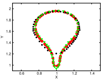
Figure 14: Shape of a Newtonian droplet rising in an Oldroyd-B fluid at $t=0.13s$. The present results ($\circ$) are compared with the results of Zainali et al.¹⁰² ($\times$) and the results of Vahabi and Sadeghy ¹⁰³ ($\triangledown$). ($Re=1.419,Eo=35.28,Wi=8.083,Bi=0,\beta=0.07,k_{\rho}=0.1,k_{\mu}=0.1,\chi=0.3,$ with $120\times 240$ grid points).

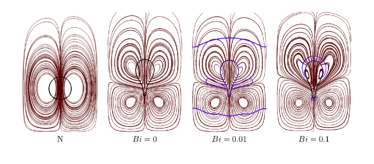
Figure 15: Streamlines for the Newtonian droplet rising in a EVP fluid and its respective shape at $t=0.13s$. Computations are performed for the Newtonian case (N), and EVP fluids with $Bi=0,0.01$ and $0.1$. The blue line denotes the solid-fluid boundary defined via contour $\mathcal{F}=0.5$. ($Re=1.419,Eo=35.28,Wi=8.083,\beta=0.07,k_{\rho}=0.1,k_{\mu}=0.1,\chi=0.3,$ and Grid: $120\times 240$).

5 Conclusion

An efficient solver has been presented for the three-dimensional direct numerical simulations of viscoelastic and elastoviscoplastic multiphase flows, expected to allow large-scale simulations also in inertial and turbulent regimes. The solver is general and applicable to non-Newtonian fluids with a dispersed phase which is either rigid or deformable (drops, bubbles and elastic particles). The fluid phases can be chosen to be simple EVP fluids following the model of Saramito⁸. The method can be later adapted to more complex EVP models.

To obtain a stable and accurate solution of the transport equations for the stresses (EVP, elastic or viscoelastic), we use a fifth-order upwinded WENO scheme for the advection term in the stress model equations. This is found to be very robust and considerably less expensive than the third-order compact upwind scheme suggested in the literature. To avoid numerical breakdown at moderate Weissenberg numbers, a local artificial diffusion can be added. We find that a local diffusion is preferable to the global diffusion which can lead to inaccurate solutions by significantly smearing out the gradients.

The interface between the continuous and dispersed phases is tracked using different approaches for different systems. For the case of deformable viscoelastic particles, we adopt an indicator function based on the local volume fraction. For droplets, we utilise a mass-conserving level set method recently developed by this group, including an accurate computation of the surface tension force based on the local curvature, and a highly efficient and scalable FFT-based pressure solver for density-contrasted flows. The overall solution approach proposed here is independent of the specific interface tracking method. The advantage of these methods is that they are fully Eulerian, efficient, accurate and portable from existing available implementations. For rigid particles, on the other hand, the interface is tracked using an immersed boundary method. In this case, the carrier phase is solved on a fixed Eulerian grid, whereas the interface is represented by a Lagrangian grid following the particle. When comparing to the conventional body fitted grid, the IBM is more simple and versatile for moving rigid bodies.

The method is first validated for single-phase elastoviscoplastic flows including the start up flow in planar channel, temporally evolving mixing layer and simple and oscillating shear flows. Then, it is applied to the sedimentation of a spherical particle in an EVP fluid, a viscoelastic drop under shear flow and a buoyancy-driven viscoelastic droplet. In all the cases mentioned above, the results obtained with our code are found to be in good agreement with previous results found in the literature. Finally, sample results are presented for a Newtonian droplet rising in an elastoviscoplastic fluid. This, and the behaviour of rigid particle suspensions in EVP fluids, will be interesting topics for future investigations.

The present methodology can also handle multi-body issues. For solid particles, we have a soft-sphere collision model ¹⁰⁸ and lubrication corrections ⁷² for short-range particle-particle and particle-wall interactions. In particular, when the gap width between two particles (or particles and wall) reduces to zero, a soft sphere collision model is activated, to calculate the normal and tangential collision force. We will extend the work on collision models to non-Newtonian fluids in the future. In the level-set method, coalescence takes place automatically. However in some cases, this phenomenon needs to be prevented. In our previous work ⁷³, a hydrodynamic model was derived for the interaction forces induced by depletion of surfactant micelles. As a future study, this model could be extended to take into account other effects of surfactants, such as diffusion at the interface and in the bulk fluid.

References

- 1 Maleki A, Hormozi S. Submerged jet shearing of visco-plastic sludge. Journal of Non-Newtonian Fluid Mechanics. 2018;252:19-27.
- 2 Gholami M, Rashedi Ahmadreza, Lenoir Nicolas, Hautemayou David, Ovarlez Guillaume, Hormozi S. Time-resolved 2D concentration maps in flowing suspensions using X-ray. Journal of Rheology. 2018;62.
- 3 Firouznia Mohammadhossein, Metzger Bloen, Ovarlez Guillaume, Hormozi Sarah. The interaction of two spherical particles in simple-shear flows of yield stress fluids. Journal of Non-Newtonian Fluid Mechanics. 2018;255:19-38.
- 4 Hormozi S, Dunbrack G, Frigaard IA. Visco-plastic sculpting. Physics of Fluids. 2014;26(9):093101.
- 5 Hormozi S, Frigaard IA. Nonlinear stability of a visco-plastically lubricated viscoelastic fluid flow. Journal of Non-Newtonian Fluid Mechanics. 2012;169:61–73.
- 6 Liu Y, Balmforth NJ, Hormozi S, Hewitt DR. Two-dimensional viscoplastic dambreaks. Journal of Non-Newtonian Fluid Mechanics. 2016;238:65–79.
- 7 Liu Y, Balmforth NJ, Hormozi S. Axisymmetric viscoplastic dambreaks and the slump test. Journal of Non-Newtonian Fluid Mechanics. 2018;258:45-57.
- 8 Saramito Pierre. A new constitutive equation for elastoviscoplastic fluid flows. Journal of Non-Newtonian Fluid Mechanics. 2007;145(1):1–14.
- 9 Bingham Eugene Cook. Fluidity and plasticity. McGraw-Hill; 1922.
- 10 Herschel WH, Bulkley R. Measurement of consistency as applied to rubber-benzene solutions. In: :621–633; 1926.
- 11 Oldroyd JG. On the formulation of rheological equations of state. In: :523–541The Royal Society; 1950.
- 12 Saramito Pierre. A new elastoviscoplastic model based on the Herschel–Bulkley viscoplastic model. Journal of Non-Newtonian Fluid Mechanics. 2009;158(1):154–161.
- 13 Ewoldt Randy H, Hosoi AE, McKinley Gareth H. New measures for characterizing nonlinear viscoelasticity in large amplitude oscillatory shear. Journal of Rheology. 2008;52(6):1427–1458.
- 14 Ewoldt Randy H, Winter Peter, Maxey Jason, McKinley Gareth H. Large amplitude oscillatory shear of pseudoplastic and elastoviscoplastic materials. Rheologica acta. 2010;49(2):191–212.
- 15 Dimitriou Christopher J, Ewoldt Randy H, McKinley Gareth H. Describing and prescribing the constitutive response of yield stress fluids using large amplitude oscillatory shear stress (LAOStress). Journal of Rheology. 2013;57(1):27–70.
- 16 Dimitriou Christopher J, McKinley Gareth H. A comprehensive constitutive law for waxy crude oil: a thixotropic yield stress fluid. Soft Matter. 2014;10(35):6619–6644.
- 17 Geri Michela, Venkatesan Ramachandran, Sambath Krishnaraj, McKinley Gareth H. Thermokinematic memory and the thixotropic elasto-viscoplasticity of waxy crude oils. Journal of Rheology. 2017;61(3):427–454.
- 18 Souza Mendes Paulo R. Dimensionless non-Newtonian fluid mechanics. Journal of Non-Newtonian Fluid Mechanics. 2007;147(1):109–116.
- 19 Bénito Sylvain, Bruneau C-H, Colin Thierry, Gay Cyprien, Molino François. An elasto-visco-plastic model for immortal foams or emulsions. The European Physical Journal E. 2008;25(3):225–251.
- 20 Fraggedakis D., Dimakopoulos Y., Tsamopoulos J.. Yielding the yield stress analysis: A thorough comparison of recently proposed elasto-visco-plastic (EVP) fluid models. Journal of Non-Newtonian Fluid Mechanics. 2016;238(Supplement C):170 - 188. Viscoplastic Fluids From Theory to Application 2015 (VPF6).
- 21 Dollet Benjamin, Graner François. Two-dimensional flow of foam around a circular obstacle: local measurements of elasticity, plasticity and flow. Journal of Fluid Mechanics. 2007;585:181–211.
- 22 Cheddadi Ibrahim, Saramito Pierre, Dollet Benjamin, Raufaste Christophe, Graner François. Understanding and predicting viscous, elastic, plastic flows. The European Physical Journal E: Soft Matter and Biological Physics. 2011;34(1):1–15.
- 23 Fraggedakis D., Dimakopoulos Y., Tsamopoulos J.. Yielding the yield-stress analysis: a study focused on the effects of elasticity on the settling of a single spherical particle in simple yield-stress fluids. Soft Matter. 2016;12:5378–5401.
- 24 Holenberg Yulia, Lavrenteva Olga M, Shavit Uri, Nir Avinoam. Particle tracking velocimetry and particle image velocimetry study of the slow motion of rough and smooth solid spheres in a yield-stress fluid. Physical Review E. 2012;86(6):066301.
- 25 Nassar Bruno, Souza Mendes Paulo R, Naccache Mônica F. Flow of elasto-viscoplastic liquids through an axisymmetric expansion–contraction. Journal of Non-Newtonian Fluid Mechanics. 2011;166(7):386–394.
- 26 Souza Mendes Paulo R, Naccache Mônica F, Varges Priscilla R, Marchesini Flavio H. Flow of viscoplastic liquids through axisymmetric expansions–contractions. Journal of Non-Newtonian Fluid Mechanics. 2007;142(1):207–217.
- 27 Cheddadi Ibrahim, Saramito Pierre, Raufaste Christophe, Marmottant Philippe, Graner François. Numerical modelling of foam Couette flows. The European Physical Journal E: Soft Matter and Biological Physics. 2008;27(2):123–133.
- 28 Cheddadi Ibrahim, Saramito Pierre, Graner François. Steady Couette flows of elastoviscoplastic fluids are nonunique. Journal of rheology. 2012;56(1):213–239.
- 29 Martins Renato da R, Furtado Giovanni M, Santos Daniel D, Frey Sérgio, Naccache Mônica F, Souza Mendes Paulo R. Elastic and viscous effects on flow pattern of elasto-viscoplastic fluids in a cavity. Mechanics Research Communications. 2013;53:36–42.
- 30 De Vita F, Rosti M E, Izbassarov D, et al. Elastoviscoplastic flows in porous media. Journal of Non-Newtonian Fluid Mechanics. 2018;258:10 - 21.
- 31 Huang PY, Feng J, Hu Howard H, Joseph Daniel D. Direct simulation of the motion of solid particles in Couette and Poiseuille flows of viscoelastic fluids. Journal of Fluid Mechanics. 1997;343:73–94.
- 32 Hwang Wook Ryol, Hulsen Martien A, Meijer Han EH. Direct simulations of particle suspensions in a viscoelastic fluid in sliding bi-periodic frames. Journal of non-newtonian fluid mechanics. 2004;121(1):15–33.
- 33 D’Avino Gaetano, Hulsen Martien A, Snijkers Frank, Vermant Jan, Greco Francesco, Maffettone Pier Luca. Rotation of a sphere in a viscoelastic liquid subjected to shear flow. Part I: Simulation results. Journal of rheology. 2008;52(6):1331–1346.
- 34 Housiadas Kostas D, Tanner Roger I. The angular velocity of a freely rotating sphere in a weakly viscoelastic matrix fluid. Physics of Fluids. 2011;23(5):051702.
- 35 Villone MM, D’Avino G, Hulsen MA, Greco F, Maffettone PL. Particle motion in square channel flow of a viscoelastic liquid: Migration vs. secondary flows. Journal of Non-Newtonian Fluid Mechanics. 2013;195:1–8.
- 36 Choi Young Joon, Hulsen Martien A, Meijer Han EH. An extended finite element method for the simulation of particulate viscoelastic flows. Journal of Non-Newtonian Fluid Mechanics. 2010;165(11):607–624.
- 37 Yoon S, Walkley MA, Harlen OG. Two particle interactions in a confined viscoelastic fluid under shear. Journal of Non-Newtonian Fluid Mechanics. 2012;185:39–48.
- 38 Janssen PJA, Baron MD, Anderson PD, Blawzdziewicz J, Loewenberg M, Wajnryb E. Collective dynamics of confined rigid spheres and deformable drops. Soft Matter. 2012;8(28):7495–7506.
- 39 D’Avino G, Hulsen MA, Maffettone PL. Dynamics of pairs and triplets of particles in a viscoelastic fluid flowing in a cylindrical channel. Computers & Fluids. 2013;86:45–55.
- 40 Oliveira IS, Noort A, Padding JT, Otter WK, Briels Willem J. Alignment of particles in sheared viscoelastic fluids. The Journal of chemical physics. 2011;135(10):104902.
- 41 Hwang Wook Ryol, Hulsen Martien A. Structure Formation of Non-Colloidal Particles in Viscoelastic Fluids Subjected to Simple Shear Flow. Macromolecular Materials and Engineering. 2011;296(3-4):321–330.
- 42 Oliveira IS Santos, Otter Wouter K, Briels Willem J. Alignment and segregation of bidisperse colloids in a shear-thinning viscoelastic fluid under shear flow. EPL (Europhysics Letters). 2013;101(2):28002.
- 43 Pasquino Rossana, D’Avino Gaetano, Maffettone Pier Luca, Greco Francesco, Grizzuti Nino. Migration and chaining of noncolloidal spheres suspended in a sheared viscoelastic medium. Experiments and numerical simulations. Journal of Non-Newtonian Fluid Mechanics. 2014;203:1–8.
- 44 Izbassarov D., Muradoglu M.. A front-tracking method for computational modeling of viscoelastic two-phase flow systems. J. Non-Newtonian Fluid Mech.. 2015;223:122 - 140.
- 45 Izbassarov Daulet, Muradoglu Metin. A computational study of two-phase viscoelastic systems in a capillary tube with a sudden contraction/expansion. Physics of Fluids. 2016;28(1):012110.
- 46 Izbassarov Daulet, Muradoglu Metin. Effects of viscoelasticity on drop impact and spreading on a solid surface. Physical Review Fluids. 2016;1(2):023302.
- 47 Villone M.M., Hulsen M.A., Anderson P.D., Maffettone P.L.. Simulations of deformable systems in fluids under shear flow using an arbitrary Lagrangian Eulerian technique. Comput. Fluids. 2014;90:88 - 100.
- 48 Villone MM, Greco F, Hulsen MA, Maffettone PL. Simulations of an elastic particle in Newtonian and viscoelastic fluids subjected to confined shear flow. Journal of Non-Newtonian Fluid Mechanics. 2014;210:47–55.
- 49 Beris AN, Tsamopoulos JA, Armstrong RC, Brown RA. Creeping motion of a sphere through a Bingham plastic. Journal of Fluid Mechanics. 1985;158:219–244.
- 50 Blackery J, Mitsoulis E. Creeping motion of a sphere in tubes filled with a Bingham plastic material. Journal of non-newtonian fluid mechanics. 1997;70(1):59–77.
- 51 Merkak Othmane, Jossic Laurent, Magnin Albert. Dynamics of particles suspended in a yield stress fluid flowing in a pipe. AIChE journal. 2008;54(5):1129–1138.
- 52 Chaparian Emad, Frigaard Ian A. Yield limit analysis of particle motion in a yield-stress fluid. Journal of Fluid Mechanics. 2017;819:311–351.
- 53 Chaparian Emad, Frigaard Ian A. Cloaking: Particles in a yield-stress fluid. Journal of Non-Newtonian Fluid Mechanics. 2017;243:47–55.
- 54 Wachs Anthony. PeliGRIFF, a parallel DEM-DLM/FD direct numerical simulation tool for 3D particulate flows. Journal of Engineering Mathematics. 2011;71(1):131–155.
- 55 Rahmani Mona, Wachs Anthony. Free falling and rising of spherical and angular particles. Physics of Fluids. 2014;26(8):083301.
- 56 Yu Zhaosheng, Wachs Anthony. A fictitious domain method for dynamic simulation of particle sedimentation in Bingham fluids. Journal of Non-Newtonian Fluid Mechanics. 2007;145(2):78–91.
- 57 Frigaard IA, Nouar C. On the usage of viscosity regularisation methods for visco-plastic fluid flow computation. Journal of Non-Newtonian Fluid Mechanics. 2005;127(1):1–26.
- 58 Tokpavi Dodji Léagnon, Magnin Albert, Jay Pascal. Very slow flow of Bingham viscoplastic fluid around a circular cylinder. Journal of Non-Newtonian Fluid Mechanics. 2008;154(1):65–76.
- 59 Putz A, Frigaard IA. Creeping flow around particles in a Bingham fluid. Journal of Non-Newtonian Fluid Mechanics. 2010;165(5):263–280.
- 60 Liu Benjamin T, Muller Susan J, Denn Morton M. Interactions of two rigid spheres translating collinearly in creeping flow in a Bingham material. Journal of non-newtonian fluid mechanics. 2003;113(1):49–67.
- 61 Maleki Amir, Hormozi S, Roustaei A, Frigaard IA. Macro-size drop encapsulation. Journal of Fluid Mechanics. 2015;769:482–521.
- 62 Saramito P. Complex Fluids. Springer; 2016.
- 63 Ovarlez Guillaume, Bertrand François, Rodts Stéphane. Local determination of the constitutive law of a dense suspension of noncolloidal particles through magnetic resonance imaging. Journal of Rheology. 2006;50(3):259–292.
- 64 Coussot Philippe, Tocquer Laurent, Lanos C, Ovarlez Guillaume. Macroscopic vs. local rheology of yield stress fluids. Journal of Non-Newtonian Fluid Mechanics. 2009;158(1):85–90.
- 65 Dagois-Bohy Simon, Hormozi Sarah, Guazzelli Élisabeth, Pouliquen Olivier. Rheology of dense suspensions of non-colloidal spheres in yield-stress fluids. Journal of Fluid Mechanics. 2015;776.
- 66 Ovarlez Guillaume, Mahaut Fabien, Deboeuf Stéphanie, Lenoir Nicolas, Hormozi Sarah, Chateau Xavier. Flows of suspensions of particles in yield stress fluids. Journal of rheology. 2015;59(6):1449–1486.
- 67 Hormozi Sarah, Frigaard IA. Dispersion of solids in fracturing flows of yield stress fluids. Journal of Fluid Mechanics. 2017;830:93–137.
- 68 Peskin C.S.. Flow patterns around heart valves: a numerical method. Journal of computational physics. 1972;10(2):252–271.
- 69 Lambert Ruth A., Picano Francesco, Breugem Wim-Paul, Brandt Luca. Active suspensions in thin films: nutrient uptake and swimmer motion. Journal of Fluid Mechanics. 2013;733:528–557.
- 70 Picano F., Breugem W. P., Brandt L.. Turbulent channel flow of dense suspensions of neutrally buoyant spheres. Journal of Fluid Mechanics. 2015;764:463–487.
- 71 Lashgari Iman, Picano Francesco, Breugem Wim Paul, Brandt Luca. Channel flow of rigid sphere suspensions: Particle dynamics in the inertial regime. International Journal of Multiphase Flow. 2016;78:12 - 24.
- 72 Ardekani M. N., Costa P., Breugem W. P., Brandt L.. Numerical study of the sedimentation of spheroidal particles. International Journal of Multiphase Flow. 2016;87:16–34.
- 73 Ge Z., J.-C. Loiseau, Tammisola O., Brandt L.. An efficient mass-preserving interface-correction level set/ghost fluid method for droplet suspensions under depletion forces. J. Comput. Phys.. 2018;353:435–459.
- 74 Rosti M. E., Brandt L.. Numerical simulation of turbulent channel flow over a viscous hyper-elastic wall. J. Fluid Mech.. 2017;830:708–735.
- 75 Joseph D. D.. Fluid dynamics of viscoelastic liquids. Springer Science & Business Media; 2013.
- 76 Dupret F., Marchal J. M.. Loss of evolution in the flow of viscoelastic fluids. Journal of Non-Newtonian Fluid Mechanics. 1986;20:143–171.
- 77 Min T., Yoo J. Y., Choi H.. Effect of spatial discretization schemes on numerical solutions of viscoelastic fluid flows. J. Non-Newtonian Fluid Mech.. 2001;100(1):27–47.
- 78 Dubief Y., Terrapon V. E., White C. M., Shaqfeh E. SG., Moin P., Lele S. K.. New answers on the interaction between polymers and vortices in turbulent flows. Flow, turbulence and combustion. 2005;74(4):311–329.
- 79 Liu X.-D., Osher S., Chan T.. Weighted essentially non-oscillatory schemes. J. Comput. Phys.. 1994;115:200–213.
- 80 Dong S., Shen J.. A time-stepping scheme involving constant coefficient matrices for phase-field incompressible flows with large density ratios. J. of Comput. Phys.. 2012;231:5788–5804.
- 81 Dodd M.S., Ferrante A.. A fast pressure-correction method for incompressible two-fluid flows. J. of Comput. Phys.. 2014;273:416–434.
- 82 Shu C.-W., Osher S.. Efficient implementation of essentially non-oscillatory shock-capturing schemes. J. Comput. Phys.. 1988;77:439–471.
- 83 Sussman M., Smereka P., Osher S.. A level set approach for computing solutions to incompressible two-phase flow. J. Comput. Phys.. 1994;114:146–159.
- 84 Chorin A.J.. Numerical solution of the Navier-Stokes equations. Math. Comput.. 1968;22:745–762.
- 85 Rosti M E, Brandt L, Mitra D. Rheology of suspensions of viscoelastic spheres: Deformability as an effective volume fraction. Physical Review Fluids. 2018;3(1):012301.
- 86 Rosti Marco E., Brandt Luca. Suspensions of deformable particles in a Couette flow. Journal of Non-Newtonian Fluid Mechanics. 2018;.
- 87 Tryggvason G, Sussman M, Hussaini M Y. Immersed boundary methods for fluid interfaces. Computational Methods for Multiphase Flow. 2007;3.
- 88 Bonet J, Wood R D. Nonlinear continuum mechanics for finite element analysis. Cambridge University Press; 1997.
- 89 Mittal R., Iaccarino G.. Immersed boundary methods. Annual Review of Fluid Mechanics. 2005;37:239–261.
- 90 Kajishima T., Takiguchi S., Hamasaki H., Miyake Y.. Turbulence structure of particle-laden flow in a vertical plane channel due to vortex shedding. JSME International Journal Series B Fluids and Thermal Engineering. 2001;44(4):526–535.
- 91 Breugem W. P., Van Dijk V., Delfos R.. Flows through real porous media: x-ray computed tomography, experiments, and numerical simulations. Journal of Fluids Engineering. 2014;136(4):040902.
- 92 Breugem W-P.. A second-order accurate immersed boundary method for fully resolved simulations of particle-laden flows. Journal of Computational Physics. 2012;231(13):4469–4498.
- 93 Uhlmann M.. An immersed boundary method with direct forcing for simulation of particulate flow. Journal of Computational Physics. 2005;209(2):448–476.
- 94 Luo K., Wang Z., Fan J., Cen K.. Full-scale solutions to particle-laden flows: Multidirect forcing and immersed boundary method. Physical Review E. 2007;76(6):066709.
- 95 Kempe T., Fröhlich J.. An improved immersed boundary method with direct forcing for the simulation of particle laden flows. Journal of Computational Physics. 2012;231(9):3663–3684.
- 96 Roma A.M., Peskin C.S., Berger M.J.. An adaptive version of the immersed boundary method. Journal of computational physics. 1999;153(2):509–534.
- 97 Waters N. D., King M. J.. Unsteady flow of an elastico-viscous liquid. Rheol. Acta. 1970;9(4):614–614.
- 98 Verhulst K., Cardinaels R., Moldenaers P., Renardy Y., Afkhami S.. Influence of viscoelasticity on drop deformation and orientation in shear flow: Part 1. Stationary states. J. Non-Newtonian Fluid Mech.. 2009;156(1):29 - 43.
- 99 Cardinaels R., Afkhami S., Renardy Y., Moldenaers P.. An experimental and numerical investigation of the dynamics of microconfined droplets in systems with one viscoelastic phase. J. Non-Newtonian Fluid Mech.. 2011;166(1):52 - 62.
- 100 Ramanujan S., Pozrikidis C.. Deformation of liquid capsules enclosed by elastic membranes in simple shear flow: large deformations and the effect of fluid viscosities. Journal of Fluid Mechanics. 1998;361:117–143.
- 101 Prieto J.L.. Stochastic particle level set simulations of buoyancy-driven droplets in non-Newtonian fluids. J. Non-Newtonian Fluid Mech.. 2015;226:16 - 31.
- 102 Zainali A., Tofighi N., Shadloo M.S., Yildiz M.. Numerical investigation of Newtonian and non-Newtonian multiphase flows using ISPH method. Computer Methods in Applied Mechanics and Engineering. 2013;254:99 - 113.
- 103 Vahabi M., Sadeghy K.. On the Use of SPH Method for Simulating Gas Bubbles Rising in Viscoelastic Liquids. Nihon Reoroji Gakkaishi. 2015;42(5):309-319.
- 104 Hysing S., Turek S., Kuzmin D., et al. Quantitative benchmark computations of two-dimensional bubble dynamics. Int. J. Num. Method. Fluids. 2009;60(11):1259–1288.
- 105 Astarita G, Apuzzo G. Motion of gas bubbles in non-Newtonian liquids. AIChE Journal. 1965;11(5):815-820.
- 106 Pillapakkam S.B., Singh P., Blackmore D., Aubry D.. Transient and steady state of a rising bubble in a viscoelastic fluid. J. Fluid Mech.. 2007;589:215–252.
- 107 Fraggedakis D., Pavlidis M., Dimakopoulos Y., Tsamopoulos J.. On the velocity discontinuity at a critical volume of a bubble rising in a viscoelastic fluid. Journal of Fluid Mechanics. 2016;789:310–346.
- 108 Costa P., Boersma B. J., Westerweel J., Breugem W. P.. Collision model for fully resolved simulations of flows laden with finite-size particles. Physical Review E. 2015;92(5):053012.