Reaction kinetics in open reactors and serial transfers between closed reactors

Abstract

Kinetic theory and thermodynamics of reaction networks are extended to the out-of-equilibrium dynamics of continuous-flow stirred tank reactors (CSTR) and serial transfers. On the basis of their stoichiometry matrix, the conservation laws and the cycles of the network are determined for both dynamics. It is shown that the CSTR and serial transfer dynamics are equivalent in the limit where the time interval between the transfers tends to zero proportionally to the ratio of the fractions of fresh to transferred solutions. These results are illustrated with a finite cross-catalytic reaction network and an infinite reaction network describing mass exchange between polymers. Serial transfer dynamics is typically used in molecular evolution experiments in the context of research on the origins of life. The present study is shedding a new light on the role played by serial transfer parameters in these experiments.

I Introduction

The regulation of self-assembly plays a critical role in biological systems, both for the emergence of life out of non-living matter and for its maintenance. Remarkable advances in the manipulation, replication, and sorting of information-rich biopolymers, such as nucleic acids Vaidya et al. (2012) or peptides,Forsythe et al. (2017) allow us to perform novel proofs of principle regarding the mechanisms prevailing to the emergence of life. In this field, chemical reaction networks of interdependent molecular species have long been considered as a central element for theoretical studies and simulations.Eigen (1971); Eigen and Schuster (1977, 1978a, 1978b); Eigen (1993); Kauffman (1993); Segré et al. (2000) Thanks to the aforementioned experimental advances,Vaidya et al. (2012); Forsythe et al. (2017) these systems are now accessible to experiments.Lincoln and Joyce (2009); Matsumura et al. (2016) Besides the relevance for the origins of life, such molecular evolution experiments suggest new chemical pathways to achieve the self-assembly of molecular elements into complex molecules and beyond into supramolecular structures.Zwaag and Meijer (2015); Zeravcic et al. (2017) Directed evolution experiments are a special kind of molecular evolution experiment, in which variations due to mutations are introduced artificially while a well-controlled selection pressure is applied.Agresti et al. (2010) This allows one to select enzymes with an improved efficiency, which is particularly attractive for industrial applications in biotechnology.Arnold and Moore (1997)

A common feature in these molecular evolution experiments is that they are open reaction networks, which are maintained out of equilibrium through incoming and outgoing fluxes of molecules or energy. Many examples of such structures exist in biology. Cytoskeletal filaments such as actin or microtubules display a rich dynamics which can only exist through a constant flux of ATP or GTP hydrolysis.Hill (1989); Padinhateeri et al. (2012); Jégou and Romet-Lemonne (2016) The same is true for larger cellular structures such as membrane protein clusters or P-granules,Brangwynne et al. (2009); Zwicker et al. (2017) which owe their special liquid-like properties to the turnover of their constituents. These systems fall into the broad class of active systems, which are presently the focus of intense research both in physics and biology.Marchetti et al. (2013) Active systems typically form dissipative structures which would not exist in the absence of non-equilibrium fluxes from the environment and which manifest very different properties than at equilibrium.Nicolis and Prigogine (1977) Therefore, an approach based on non-equilibrium statistical mechanics and thermodynamics is required to describe them. Building on the well established framework of nonequilibrium thermodynamics Prigogine (1967); de Groot and Mazur (1984) and on more recent progress in stochastic thermodynamics, a generic and comprehensive theory of open chemical networks has been recently developed.Polettini and Esposito (2014); Rao and Esposito (2016) In previous work, this theoretical framework has been used to analyze a mass-exchange model of polymers with identical monomers in a closed system Lahiri et al. (2015) and an open version of the same model, in which chemostats fix the concentrations of polymers of certain length and as a result drive the system out of equilibrium.Rao et al. (2015) When different monomer types are present, an even richer dynamics of recombination between polymer chains is possible due to the interplay between polymer lengths and polymer sequences.Blokhuis and Lacoste (2017)

There exist several approaches to drive a reaction network out of equilibrium. One of them is the continuous-flow stirred tank reactor (CSTR), in which a well-stirred solution is continuously fed by reactants while keeping constant its volume with a compensating outflow.Aris (1989); Bergé et al. (1984); Vidal and Lemarchand (1988); Nicolis (1995); Epstein and Pojman (1998)

In the experiment of Ref. Vaidya et al., 2012, a mixture of interdependent biopolymers evolves through serial transfers, in which a part of the solution of interest is periodically transferred to a nutrient medium, from which the solution of interest draws reactant molecules and energy. Chemical systems evolving by serial transfers have similarities with systems evolving in CSTRs, but it is not clear whether the two dynamics are completely equivalent from a kinetic or thermodynamic point of view. CSTRs can exhibit a large range of dynamic phenomena, such as stationary, oscillatory, multi-stable or chaotic Vidal and Lemarchand (1988); Aris (1989); Scott (1991) and it is natural to ask whether all these regimes are possible in a reactor evolving instead by serial transfers. Let us also mention that a setup somehow similar to CSTRs also exists under the name of chemostats in studies of the metabolism of cells: in such bioreactors, a population of cells is maintained in an exponentially growing phase by the injection of nutrients into the system.Salman et al. (2012)

In this paper, we compare the kinetic and thermodynamic descriptions of open reactors (CSTRs) with that obtained in the case of serial transfers between closed reactors. We illustrate our results with a study of the polymer mass-exchange model of Ref. Rao et al., 2015, except that now the system is not driven out of equilibrium by chemostats as considered in Refs. Polettini and Esposito, 2014; Rao and Esposito, 2016, but by matter fluxes in a CSTR configuration. This paper is organized as follows: in Sec. II, we study the kinetics and thermodynamics of CSTRs, which is then illustrated with a couple of examples of chemical reactions, then in Sec. III we carry out the corresponding study for the case of serial transfer dynamics between closed reactors. The conclusion is drawn in Sec. IV.

II Continuous-flow stirred tank reactor

II.1 Kinetic equations of the CSTR

Continuous-flow stirred tank reactors are open reactors with a continuous feed of reactants and an outflow in order to keep the volume constant inside the reactor (see Fig. 1). The reactants are pumped into the reactor at given controlled concentrations $c_{k,{\rm in}}$. The solution in the reactor is well stirred so that the concentrations of the different species can be supposed to remain uniform inside the volume of the reactor. In order to establish the evolution equations of the concentrations in the CSTR, we use the balance equations of the concentrations $c_{k}$ in the flow:

$$\partial_{t}c_{k}+\boldsymbol{\nabla}\cdot\left(c_{k}{\bf v}+{\bf j}_{k}\right)=\sum_{i}\nu_{ki}w_{i}\,,$$ (1)

expressed in terms of the fluid velocity $\bf v$, the diffusive current density of species $k$ given by Fick’s law ${\bf j}_{k}=-D_{k}\boldsymbol{\nabla}c_{k}$, the stoichiometric coefficient $\nu_{ki}$ of species $k$ in the reaction $i$, and the rate $w_{i}$ of reaction $i$. The different species are passively advected by the turbulent velocity field $\bf v$ of the flow. By stirring, the concentrations rapidly become uniform so that the Fickian diffusive current densities are soon negligible ${\bf j}_{k}\simeq 0$. Integrating the balance equation (1) over the volume $V$ of the reactor, we find

$$\int_{V}\partial_{t}\,c_{k}\,dV+\int_{\partial V}c_{k}{\bf v}\cdot d{\bf A}=\int_{V}\sum_{i}\nu_{ki}w_{i}\,dV\,,$$ (2)

where $d{\bf A}$ is the surface element of integration on the border $\partial V$ of the volume $V$. The surface integral has contributions from the inflow tube of species $k$ entering with concentration $c_{k,{\rm in}}$ and the outflow tube where the species $k$ exits at the uniform concentration $c_{k}$ resulting from stirring:

$$\int_{\partial V}c_{k}{\bf v}\cdot d{\bf A}=\int_{\partial V_{k,{\rm in}}}c_{k}{\bf v}\cdot d{\bf A}+\int_{\partial V_{\rm out}}c_{k}{\bf v}\cdot d{\bf A}\,.$$ (3)

Since the concentrations can be supposed to be uniform at entry and exit, we get

$$\int_{\partial V}c_{k}{\bf v}\cdot d{\bf A}=-\phi_{k,{\rm in}}\,c_{k,{\rm in}}+\phi_{\rm out}\,c_{k}$$ (4)

in terms of the ingoing flux $\phi_{k,{\rm in}}=\int_{\partial V_{k,{\rm in}}}{\bf v}\cdot d{\bf A}$ of the solution in the tube bringing species $k$ into the reactor and the exit flux $\phi_{\rm out}=\int_{\partial V_{\rm out}}{\bf v}\cdot d{\bf A}$ of the stirred solution. These fluxes are in units of m³ per second, and depend on the section areas of the injection and exit tubes. The volume of the solution inside the reactor being preserved, we have that $\phi_{\rm out}=\sum_{k}\phi_{k,{\rm in}}$. Since the concentrations are uniform inside the reactor, Eq. (2) divided by the volume $V$ becomes

$$\frac{dc_{k}}{dt}=\sum_{i}\nu_{ki}\,w_{i}+\frac{1}{\tau}(c_{k0}-c_{k})\,,$$ (5)

where $\tau\equiv V/\phi_{\rm out}$ is the mean residence time of the species inside the reactor, and

$$c_{k0}\equiv\frac{\phi_{k,{\rm in}}}{\phi_{\rm out}}\,c_{k,{\rm in}}$$ (6)

are the injected concentrations of reactants reported to the whole volume. Both the residence time $\tau$ and the injected concentrations $c_{k0}$ are control parameters.

Figure 1: Schematic representation of a continuous-flow stirred tank reactor (CSTR). The dashed line depicts a fictitious surface delimiting the volume $V$ of the reactor.

The evolution equations for the concentrations form a set of ordinary differential equations, which are typically nonlinear. In the limit where the residence time becomes very long, the last term of Eq. (5) becomes negligible and we recover the kinetic equations in a closed reactor, the so-called batch reactor,Epstein and Pojman (1998) in which case the concentrations will sooner or later reach their equilibrium value. In the other limit where the residence time is very short, the last term dominates so that the concentrations remain nearly equal to their value at injection: $c_{k}\simeq c_{k0}$. In between, the concentrations may manifest a rich variety of different stationary, oscillatory, or chaotic behaviors in some autocatalytic or cross-catalytic reaction networks.Bergé et al. (1984); Vidal and Lemarchand (1988); Scott (1991); Nicolis (1995); Epstein and Pojman (1998)

II.2 Thermodynamics

A typical CSTR is functioning under atmospheric pressure and at room temperature if the reactions are not too exothermic. Under these conditions, the relevant thermodynamic potential is Gibbs’ free energy $G$. We assume local thermodynamic equilibrium for every element of the solution and consider the free energy density:

$$g_{V}=\sum_{k}\mu_{k}\,c_{k}\,,$$ (7)

where $\mu_{k}$ is the chemical potential of species $k$.

Using Eq. (7) together with Gibbs’ fundamental relation per unit volume

$$dg_{V}=-s_{V}dT+dP+\sum_{k}\mu_{k}dc_{k}\,,$$ (8)

where $s_{V}$ is the entropy density, $T$ the temperature, and $P$ the pressure, one obtains the Gibbs-Duhem relation

$$s_{V}dT-dP+\sum_{k}c_{k}d\mu_{k}=0\,.$$ (9)

Using Eq. (9) under isothermal and isobaric conditions, one finds that

$$\sum_{k}c_{k}d\mu_{k}=0.$$ (10)

Since the solution is well stirred, it is quasi homogeneous in the bulk of the tank, and the time evolution of the Gibbs free energy follows that of the concentrations of the various species. Using Eqs. (7)-(10), one obtains

$$\frac{dg_{V}}{dt}=\sum_{k}\mu_{k}\frac{dc_{k}}{dt},$$ (11)

Now, using Eq. (5) for the concentrations, the time evolution of the free energy density then becomes

$$\frac{dg_{V}}{dt}=\sum_{ki}\mu_{k}\nu_{ki}w_{i}+\frac{1}{\tau}\sum_{k}\mu_{k}\left(c_{k0}-c_{k}\right)\,.$$ (12)

According to the mass action law,Nicolis (1995) the reaction rates are proportional to the concentrations of all the species entering in the reaction. It is convenient to make the distinction between the forward and reversed reactions so that

$$w_{\pm i}=k_{\pm i}\prod_{k}\left(\frac{c_{k}}{c^{0}}\right)^{\nu_{ki}^{(\pm)}}\,,$$ (13)

where $k_{\pm i}$ are the rate constants, $\nu_{ki}^{(\pm)}$ the numbers of molecules entering the forward or the reversed reaction, and $c^{0}$ the standard concentration of one mole per liter. The stoichiometric coefficient is thus given by $\nu_{ki}=\nu_{ki}^{(-)}-\nu_{ki}^{(+)}$, while $w_{i}=w_{+i}-w_{-i}$. In a dilute solution, the chemical potentials of the solute species are given by $\mu_{k}=\mu_{k}^{0}+RT\ln(c_{k}/c^{0})$ where $R$ is the molar gas constant. Now, the ratio of the rate constants is related to the standard free energy of the reaction according to

$$\frac{k_{+i}}{k_{-i}}=\exp\Big{(}-\sum_{k}\frac{\mu_{k}^{0}\nu_{ki}}{RT}\Big{)}\,.$$ (14)

The entropy production rate of the reactions is given by

$$\sigma = -\frac{1}{T}\sum_{ki}\mu_{k}\nu_{ki}w_{i},$$ (15)

$$= R\sum_{i}\left(w_{+i}-w_{-i}\right)\ln\frac{w_{+i}}{w_{-i}}\geq 0\,,$$

which is always non-negative.

Now, combining Eq. (15) with Eq. (12), the time evolution of the free energy density becomes

$$\frac{dg_{V}}{dt}=-T\sigma+\frac{1}{\tau}\left(\gamma_{0}-g_{V}\right)\,,$$ (16)

where we have introduced the following quantity

$$\gamma_{0}=\sum_{k}\mu_{k}\,c_{k0}.$$ (17)

In a closed reactor where $\tau$ is infinite, the free energy will decrease towards its minimal value. However, in an open reactor where $\tau$ is finite, the free energy does not need to reach its minimal value. In this regard, nonequilibrium stationary, oscillatory, or chaotic regimes can be sustained in an open reactor.Prigogine (1967); Nicolis (1995)

The term $\left(\gamma_{0}-g_{V}\right)/\tau$ in Eq. (16) has no definite sign, except in a stationary state where it is equal to the dissipation produced by the chemical reactions and therefore must be positive. In this case, it is sufficient to know the Gibbs free energies of incoming and outgoing chemical species in order to know the dissipation associated with chemical reactions within the reactor.

II.3 General properties of reaction networks in a CSTR

Reaction network theory allows us to obtain key properties such as the conservation laws and the cycles, which determine the behavior of the stationary states. These properties are known for chemostatted systems,Rao and Esposito (2016); Polettini and Esposito (2014) and an important issue is to understand how they differ in a CSTR. We note that the cycles defined in reaction network theory should not be confused with the limit cycles of nonlinear dynamics. The former are defined as the right null eigenvectors of the stoichiometric matrix,Rao and Esposito (2016) while the latter are periodic solutions for the ordinary differential equations of the reaction network corresponding to periodic oscillations.Nicolis and Prigogine (1977); Nicolis (1995)

The equations (5) ruling the time evolution of the concentrations can be rewritten in matrix form as follows:

$$\frac{d{\bf c}}{dt}=\boldsymbol{\nu}\cdot{\bf w}+\frac{1}{\tau}\left({\bf c}_{0}-{\bf c}\right),$$ (18)

in terms of the $s$-dimensional vectors $\bf c$ and ${\bf c}_{0}$ of concentrations and injected concentrations, the $r\times s$ matrix $\boldsymbol{\nu}$ of stoichiometric coefficients, and the $r$-dimensional vector of reaction rates $\bf w$, where $s$ is the number of species and $r$ the number of reactions in the network.

In the limit $\tau\to\infty$, we recover the case of a closed reactor.Rao and Esposito (2016); Polettini and Esposito (2014) In a stationary state, we have $\boldsymbol{\nu}\cdot{\bf w}=0,$ implying that ${\bf w}$ can be decomposed in the basis of right null eigenvectors ${\bf e}_{\gamma}$, which are called cycles: ${\bf w}=\sum_{\gamma}w_{\gamma}{\bf e}_{\gamma}$.

The rank of the stoichiometry matrix of the closed reactor can be written as

$${\rm rank}(\boldsymbol{\nu})=r-o=s-l\,,$$ (19)

where $o={\rm dim\,ker}(\boldsymbol{\nu})$ is the number of cycles, and $l={\rm dim\,coker}(\boldsymbol{\nu})$ the number of conserved quantities. The quantities that are conserved in a closed reactor are defined as

$$L\equiv\boldsymbol{\ell}\cdot{\bf c}\,,$$ (20)

with a vector $\boldsymbol{\ell}$ such that

$$\boldsymbol{\ell}\cdot\boldsymbol{\nu}=0\,.$$ (21)

In an open reactor where $\tau$ is finite, such quantities are no longer conserved. Instead, they converge asymptotically towards their value defined for the injected concentrations:

$$L_{0}=\boldsymbol{\ell}\cdot{\bf c}_{0}\,.$$ (22)

Indeed, applying the vector $\boldsymbol{\ell}$ to Eq. (18), we find that

$$\frac{dL}{dt}=\frac{1}{\tau}(L_{0}-L)\,,$$ (23)

the solution of which is given by

$$L(t)=L(0)\,{\rm e}^{-t/\tau}+L_{0}\left(1-{\rm e}^{-t/\tau}\right).$$ (24)

It is important to emphasize that all conservation laws are broken in a CSTR.

We can also recover this result using the full stoichiometry matrix of the CSTR. In an open reactor, the reaction network also includes the $s$ reactions of rates $\left({\bf c}_{0}-{\bf c}\right)/\tau$ so that the total number of reactions becomes $r^{\prime}=r+s$, while the matrix of stoichiometric coefficients should be extended towards a $r^{\prime}\times s$ matrix with $r^{\prime}=r+s$. This means that the new stoichiometry matrix of the CSTR reads

$$\boldsymbol{\nu}^{\prime}=\left(\boldsymbol{\nu},\boldsymbol{I}\right),$$ (25)

where $\boldsymbol{I}$ is the identity matrix $s\times s$. Therefore Eq. (18) becomes

$$\frac{d{\bf c}}{dt}=\boldsymbol{\nu}^{\prime}\cdot{\bf w^{\prime}},$$ (26)

with the flow rate ${\bf w^{\prime}}=\left({\bf w},{\bf\tilde{w}}\right)^{\rm T}$ a column matrix of dimension $1\times r^{\prime}$ with ${\bf\tilde{w}}=({\bf c}_{0}-{\bf c})/\tau$.

In an open reactor, we also get

$${\rm rank}(\boldsymbol{\nu}^{\prime})=r^{\prime}-{\rm dim\,ker}(\boldsymbol{\nu}^{\prime})=s-{\rm dim\,coker}(\boldsymbol{\nu}^{\prime})\,.$$ (27)

The number of conserved quantities is now equal to zero $l^{\prime}={\rm dim\,coker}(\boldsymbol{\nu}^{\prime})=0$ so that the number of cycles is equal to the number of reactions in the original network: $o^{\prime}={\rm dim\,ker}(\boldsymbol{\nu}^{\prime})=r$. Therefore, there are $o^{\prime}-o=r-o=s-l$ cycles of the open network that were not already present in the corresponding closed network. For chemostatted systems, such cycles have been called emergent cycles.Polettini and Esposito (2014); Rao and Esposito (2016)

Here, we choose to call these cycles external cycles, because they involve the flow rates ${\bf\tilde{w}}$ which are specific to the CSTR. The other cycles are called internal. A general cycle $\bf{e}^{\prime}$ can be split into network components and flow components as $\bf{e}^{\prime}=(\bf{e},{\bf\tilde{e}})^{\rm T}$. This cycle obeys $\boldsymbol{\nu}^{\prime}\cdot{\bf e}^{\prime}=\boldsymbol{\nu}\cdot{\bf e}+{\bf\tilde{e}}=0$. Here we can make the distinction between internal cycles ${\bf e}_{\gamma}$ previously defined for the network of the closed reactor which are such that $\boldsymbol{\nu}\cdot{\bf e}_{\gamma}=0$ and ${\bf\tilde{e}}_{\gamma}=0$; and external cycles ${\bf e}_{\alpha}$ which are such that ${\bf\tilde{e}}_{\alpha}=-\boldsymbol{\nu}\cdot{\bf e}_{\alpha}\neq 0$.

As far as the thermodynamic description of the system is concerned, Eq. (16) becomes

$$\frac{dg_{V}}{dt}=\sum_{ki}\mu_{k}\nu^{\prime}_{ki}w^{\prime}_{i}\,,$$ (28)

within the framework of the extended network. In a stationary state, the entropy production rate of Eq. (15) may be rewritten as:

$$\sigma = -\frac{1}{T}\,\boldsymbol{\mu}\cdot\boldsymbol{\nu}\cdot{\bf w}=-\frac{1}{T}\sum_{\lambda}w_{\lambda}\,\boldsymbol{\mu}\cdot\boldsymbol{\nu}\cdot{\bf e}_{\lambda},$$ (29)

$$= -\frac{1}{T}\sum_{\alpha}w_{\alpha}\,\boldsymbol{\mu}\cdot\boldsymbol{\nu}\cdot{\bf e}_{\alpha},$$

$$= \frac{1}{T}\sum_{\alpha}w_{\alpha}\,\boldsymbol{\mu}\cdot{\bf\tilde{e}}_{\alpha}\geq 0.$$

This shows that in this case the entropy production rate can be written as a sum of contribution from external cycles denoted with the index $\alpha$ only. A similar property was reported in the case of chemostatted systems.Polettini and Esposito (2014); Rao and Esposito (2016)

II.4 Illustrative examples

Here, we present two illustrative examples of the above framework. The first example is a network of small size taken from Ref. Polettini and Esposito, 2014, and the second one is a larger network describing polymers with a mass-exchange process taken from Ref. Rao et al., 2015.

II.4.1 Example with a finite network

The set of reactions in the first example are

$$\ce{A+B<=>[1]C},\qquad\qquad w_{1}=k_{+1}[\ce{A}][\ce{B}]-k_{-1}[\ce{C}],$$ (30)

$$\ce{C<=>[2]B+D},\qquad\qquad w_{2}=k_{+2}[\ce{C}]-k_{-2}[\ce{B}][\ce{D}],$$ (31)

$$\ce{B+D<=>[3]E},\qquad\qquad w_{3}=k_{+3}[\ce{B}][\ce{D}]-k_{-3}[\ce{E}],$$ (32)

$$\ce{E<=>[4]A+B},\qquad\qquad w_{4}=k_{+4}[\ce{E}]-k_{-4}[\ce{A}][\ce{B}].$$ (33)

The stoichiometry matrix of this network is then

$$\boldsymbol{\nu}=\left(\begin{array}[]{rrrr}-1&0&0&1\\ -1&1&-1&1\\ 1&-1&0&0\\ 0&1&-1&0\\ 0&0&1&-1\end{array}\right),$$ (39)

and the corresponding hypergraph is shown in Fig. 2.Rao and Esposito (2016)

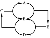
Figure 2: Hypergraph of the closed chemical network (30)-(33).

As shown in Ref. Polettini and Esposito, 2014, this network has $l=2$ conserved quantities $L_{1}=[\ce{B}]+[\ce{C}]+[\ce{E}]$ and $L_{2}=[\ce{A}]+[\ce{C}]+[\ce{D}]+[\ce{E}]$. There is only one cycle ($o=1$), with a null right eigenvector $(1,1,1,1)^{\rm T}$.

For the open reactor network, the stoichiometry matrix $\boldsymbol{\nu}^{\prime}$ is obtained from Eq. (25), its rank is 5, it has $o^{\prime}=4$ cycles, $l^{\prime}=0$ conserved quantities, and $s-l=3$ new cycles. The cycles are the old cycle ${\bf e}_{1}=(1,1,1,1,0,0,0,0,0)^{\rm T}$ and the three new cycles ${\bf e}_{2}=(1,1,0,0,1,0,0,-1,0)^{\rm T}$, ${\bf e}_{3}=(0,1,1,0,0,0,1,0,-1)^{\rm T}$, and ${\bf e}_{4}=(0,0,1,1,-1,0,0,1,0)^{\rm T}$. The new cycles are represented in Fig. 3. This representation makes it clear that hypergraphs depicting the new cycles of the open network are built from the hypergraph of the closed network by removing some reactions and chemical species. Then the remaining pieces are connected together using a special symbol $\phi$, which is introduced for this purpose and which describes new reaction pathways involving the exterior of the CSTR.

We note that the hypergraphs in Figs. 2 and 3 depend on the reaction network, but not on the concentration values of the involved species.

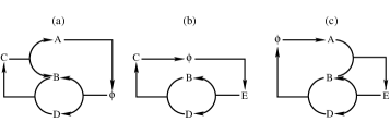
Figure 3: Hypergraphs of the three new cycles in the open version of the chemical network represented in Fig. 2. Here $(a)$, $(b)$ and $(c)$ correspond to the cycles ${\bf e}_{2}$, ${\bf e}_{3}$ and ${\bf e}_{4}$ respectively. Note the appearance of the symbol $\phi$ which is a notation for new reactions involving the inflow and outflow of the CSTR.

II.4.2 Example with an infinite network

We now move to a more complex reaction network, namely the model of polymers undergoing a mass-exchange process taken from Ref. Rao et al., 2015. In this model, two polymers of mass $n$ and $m$ interact with the reaction

$$(n)+(m)\ce{<=>[\kappa]}(n+1)+(m-1),\qquad{\rm for}\quad n\geq 1,\ m\geq 2.$$ (40)

In an open reactor, the kinetic equations can be written in the form:

$$\frac{dc_{k}}{dt}=\frac{1}{2}\sum_{n\geq 1,m\geq 2}\nu_{k,nm}\,w_{nm}+\frac{1}{\tau}(c_{k,0}-c_{k})\quad\quad{\rm for}\quad k\geq 1,$$ (41)

with the stoichiometric coefficients $\nu_{k,nm}=\delta_{k,n+1}+\delta_{k,m-1}-\delta_{k,n}-\delta_{k,m}$ and the rates $w_{nm}=\kappa c_{n}c_{m}-\kappa c_{n+1}c_{m-1}$ obeying the mass action law.

In the closed reactor ($\tau=\infty$), this network has two conserved quantities: the total concentration $c\equiv\sum_{k=1}^{\infty}c_{k}$ and the total number of monomeric units $M=\sum_{k=1}^{\infty}k\,c_{k}$. In the open reactor, these quantities are no longer conserved because they obey the equations

$$\frac{dc}{dt} = \frac{1}{\tau}\left(c_{0}-c\right)\,,$$ (42)

$$\frac{dM}{dt} = \frac{1}{\tau}\left(M_{0}-M\right)\,,$$ (43)

so that they converge asymptotically in time towards their value $c_{0}$ or $M_{0}$ fixed by the inlet concentrations.

Although the reaction network is infinite, it can be truncated by considering a finite number $s$ of species. In this case, the reactions and the cycles can be enumerated using the list of all the reactions:

$$\ce{1+2<=>2+1}\,,\quad\ce{2+3<=>3+2}\,,\quad\ce{3+4<=>4+3}\,,\ \dots$$

$$\ce{1+3<=>2+2}\,,\quad\ce{2+4<=>3+3}\,,\ \dots$$

$$\ce{1+4<=>2+3}\,,\ \dots$$

$$\qquad\quad\vdots$$ (44)

In the closed reactor, the number of reactions involving $s$ species is thus equal to

$$r=\frac{1}{2}s(s-1)\,.$$ (45)

Since there are $l=2$ conserved quantities in the closed reactor, Eq. (19) thus shows that the number of cycles is equal to

$$o=r-s+2=\frac{1}{2}(s-1)(s-2)+1\,.$$ (46)

Accordingly, these numbers are increasing quadratically with the number $s$ of species.

In the open reactor, the reactions include the rates $\tilde{w}_{k}=(c_{k0}-c_{k})/\tau$ due to the flow so that the number of reactions involving $s$ species is now given by

$$r^{\prime}=r+s=\frac{1}{2}s(s+1)\,.$$ (47)

There are no conserved quantities $l^{\prime}=0$ and the number of cycles is here equal to

$$o^{\prime}=o+s-2=r=\frac{1}{2}s(s-1)\,.$$ (48)

Therefore, opening the reactor only adds a number of new cycles $s-2$ that is increasing linearly with the number of species, while the total number of cycles of the open system is increasing quadratically with the number of species.

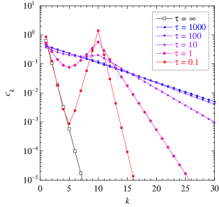
Figure 4: Stationary distributions of the oligomer concentrations $\{c_{k}\}$ for the mass-exchange process with the rate constant $\kappa=1$ in a CSTR with the injection of monomers and 10-mers at the inlet concentrations $c_{1,0}=1$ and $c_{10,0}=2$ for different values of the residence time $\tau$. If $\tau=\infty$, the reactor is closed and the stationary distribution is the equilibrium one (open squares). If $\tau$ is finite, the reactor is open and out of equilibrium (filled symbols).

In the CSTR, all the concentrations remain bounded in time. This rules out the possibility to observe an “unbalanced phase”, such as the unbounded growth phase reported in Ref. Rao et al., 2015 in a variant of this mass-exchange model, which was driven out-of-equilibrium by chemostats fixing the concentrations of polymers of certain lengths. In that model, the total concentration $c$ increased linearly in time and the total number of monomers $M$ increased quadratically. In contrast, in a CSTR both quantities remain bounded in time, a property which follows generally from Eq. (23).

In Fig. 4, we show the stationary distribution of concentrations in a CSTR for different values of the residence time $\tau$ by injecting monomers at the concentration $c_{1,0}$ and oligomers of length $l=10$ at the concentration $c_{10,0}$. The kinetic equations are integrated with a Runge-Kutta algorithm of orders 4 and 5 with variable steps from the initial distribution $c_{k}(0)=\exp(-k^{2}/2)$. The distribution is plotted after a time interval $t=1000$ if $\tau=\infty,0.1,1,10$, after $t=10000$ if $\tau=100$, and after $t=50000$ if $\tau=1000$, when stationarity is numerically reached. If $\tau=\infty$, the reactor is closed so that the concentrations reach their equilibrium exponential distribution

$$c_{k,{\rm eq}}=\frac{c(0)^{2}}{M(0)}\left[1-\frac{c(0)}{M(0)}\right]^{k-1},$$ (49)

determined by the initial values of the two invariant quantities $c(0)=0.7533$ and $M(0)=0.9119$, so that $c_{k,{\rm eq}}=3.58\times 0.174^{k}$. In contrast, under nonequilibrium conditions if $\tau$ is finite, the distribution deviates from being purely exponential and it even becomes bimodal with peaks at $k=1$ and $k=10$ if the open reactor is strongly out of equilibrium with a small enough residence time $\tau$. Nevertheless, the distribution is always exponential beyond the largest injected concentration $c_{10,0}$, as shown in Appendix A. In the open reactor, the distribution no longer depends on the initial conditions but on the values of the injected concentrations.

III Serial transfers between closed reactors

Now, we consider the dynamics of the reaction network in a typical serial transfer experiment.Vaidya et al. (2012)

III.1 Time evolution of the concentrations

At every transfer, a fraction $f$ of the solution volume $V$ is transferred to another closed reactor already containing a fresh solution of volume $(1-f)V$ with reactants at the concentrations $c_{k0}$ as illustrated in Fig. 5.

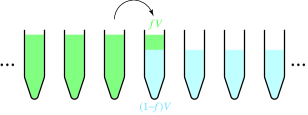
Figure 5: Schematic representation of a serial transfer experiment in which a volume $fV$ of the solution of interest (green) is transferred repeatedly into a fresh solutions of volume $(1-f)V$ (blue).

Let $\mathscr{T}$ be the time interval between two transfers. During this time interval, the reactor is closed so that the concentrations evolves according to

$$\frac{d{\bf c}}{dt}=\boldsymbol{\nu}\cdot{\bf w}\,.$$ (50)

Let ${\bf c}(n{\mathscr{T}}-0)$ be the concentrations just before the previous transfer. The concentrations just after the transfer and stirring are thus given by

$${\bf c}(n{\mathscr{T}}+0)=(1-f)\,{\bf c}_{0}+f\,{\bf c}(n{\mathscr{T}}-0)\,.$$ (51)

Thereafter, the concentrations evolves according to

$${\bf c}\left(t\right)={\bf c}(n{\mathscr{T}}+0)+\int_{n{\mathscr{T}}}^{t}\boldsymbol{\nu}\cdot{\bf w}\left[{\bf c}(t^{\prime})\right]\,dt^{\prime}$$ (52)

with $n{\mathscr{T}}+0<t<n{\mathscr{T}}+{\mathscr{T}}-0$. The concentrations just before the next transfer are thus given by

$${\bf c}(n{\mathscr{T}}+{\mathscr{T}}-0) = (1-f)\,{\bf c}_{0}+f\,{\bf c}(n{\mathscr{T}}-0)$$ (53)

$$+\int_{n{\mathscr{T}}}^{(n+1){\mathscr{T}}}\boldsymbol{\nu}\cdot{\bf w}\left[{\bf c}(t)\right]\,dt\,,$$

which defines a mapping ${\bf c}_{n+1}=\boldsymbol{\Phi}({\bf c}_{n})$ from ${\bf c}_{n}\equiv{\bf c}(n{\mathscr{T}}-0)$ to ${\bf c}_{n+1}\equiv{\bf c}(n{\mathscr{T}}+{\mathscr{T}}-0)$. A similar mapping can be obtained for the concentrations after the transfers.

Let us suppose that the transfers are quickly repeated every small time interval ${\mathscr{T}}=\Delta t$. As a consequence of Eq. (53), we get the approximate ordinary differential equations:

$$\frac{\Delta{\bf c}}{\Delta t}\simeq\frac{1-f}{\Delta t}\,({\bf c}_{0}-{\bf c}_{n})+\boldsymbol{\nu}\cdot{\bf w}\left[(1-f)\,{\bf c}_{0}+f\,{\bf c}_{n}\right]\,,$$ (54)

where $\Delta{\bf c}={\bf c}_{n+1}-{\bf c}_{n}$. Introducing the effective residence time

$$\tau\equiv\frac{\Delta t}{1-f}\,,$$ (55)

we recover in the limit $\Delta t\to 0$ the kinetic equations of the concentrations in a CSTR:

$$\frac{d{\bf c}}{dt}=\boldsymbol{\nu}\cdot{\bf w}({\bf c})+\frac{1}{\tau}\left({\bf c}_{0}-{\bf c}\right)\,.$$ (56)

If $f=1-{\mathscr{T}}/\tau$ in the limit ${\mathscr{T}}\to 0$, an experiment of serial transfers between closed reactors is thus similar to an experiment in a CSTR. Therefore, similar nonequilibrium regimes are expected in both experiments under comparable conditions.

III.2 Thermodynamics

Let us follow Gibbs’ free energy during the time evolution. Before the transfer at time $n{\mathscr{T}}$, the free energy density of the solution in the volume $V$ is $g_{V}\left[{\bf c}\left(n{\mathscr{T}}-0\right)\right]$. After the transfer of the volume $fV$ of solution into the volume $(1-f)V$ of fresh solution and the mixing of both, the free energy density becomes $g_{V}\left[f{\bf c}\left(n{\mathscr{T}}-0\right)+(1-f){\bf c}_{0}\right]$. Thereafter, the free energy density changes in time since the concentrations evolve according to Eq. (50) in the closed reactor. At the end of the time interval $n{\mathscr{T}}<t<n{\mathscr{T}}+{\mathscr{T}}$, the free energy density has thus become

$$g_{V}\left[{\bf c}\left(n{\mathscr{T}}+{\mathscr{T}}-0\right)\right] = g_{V}\left[f{\bf c}\left(n{\mathscr{T}}-0\right)+(1-f){\bf c}_{0}\right]$$ (57)

$$+\int_{n{\mathscr{T}}}^{(n+1){\mathscr{T}}}dt\,\dot{g}_{V}\left[{\bf c}(t)\right],$$

where $\dot{g}_{V}=\boldsymbol{\mu}\cdot\boldsymbol{\nu}\cdot{\bf w}$ is the time derivative of the free energy in the closed reactor given by Eq. (12) with $\tau=\infty$. The process repeats itself at every time interval.

In the limit where ${\mathscr{T}}=\Delta t\to 0$ with $f=1-\Delta t/\tau$, using the same notation ${\bf c}_{n}\equiv{\bf c}(n{\mathscr{T}}-0)$ as above, Eq. (57) becomes

$$g_{V}({\bf c}_{n+1}) = g_{V}\left[{\bf c}_{n}+\frac{\Delta t}{\tau}({\bf c}_{0}-{\bf c}_{n})\right]$$ (58)

$$+\Delta t\,\boldsymbol{\mu}({\bf c}_{n})\cdot\boldsymbol{\nu}\cdot{\bf w}({\bf c}_{n})+O(\Delta t^{2})\,.$$

Since $\boldsymbol{\mu}=\partial g_{V}/\partial{\bf c}$, the previous equation becomes

$$g_{V}({\bf c}_{n+1}) = g_{V}({\bf c}_{n})+\frac{\Delta t}{\tau}\,\boldsymbol{\mu}({\bf c}_{n})\cdot({\bf c}_{0}-{\bf c}_{n})$$ (59)

$$+\Delta t\,\boldsymbol{\mu}({\bf c}_{n})\cdot\boldsymbol{\nu}\cdot{\bf w}({\bf c}_{n})+O(\Delta t^{2})\,.$$

In the limit $\Delta t\to 0$, we thus find the differential equation

$$\frac{dg_{V}}{dt}=\boldsymbol{\mu}({\bf c})\cdot\boldsymbol{\nu}\cdot{\bf w}({\bf c})+\frac{1}{\tau}\,\boldsymbol{\mu}({\bf c})\cdot({\bf c}_{0}-{\bf c})\,,$$ (60)

which is the same as Eq. (12) for the time evolution of the free energy in the CSTR.

In the limit $\Delta t\to 0$, there is thus equivalence between the dynamics in the CSTR and the time evolution in a serial transfer experiment.

III.3 General properties of the reaction network in serial transfers

The considerations of Subsec. II.3 extends to reaction networks in serial transfers between closed reactors. Here, a stationary state corresponds to a fixed point ${\bf c}_{n}={\bf c}_{*}=\boldsymbol{\Phi}({\bf c}_{*})$ of the mapping defined by Eq. (53).

As in the case of the CSTR, conserved quantities of the closed network, namely quantities of the form $L=\boldsymbol{\ell}\cdot{\bf c}$ are no longer conserved in the open reactor. Instead, their dynamics follows a simple relaxation equation

$$L\left(n{\mathscr{T}}+{\mathscr{T}}-0\right)=(1-f)L_{0}+fL\left(n{\mathscr{T}}-0\right),$$ (61)

which is the counterpart of Eq. (23). At the fixed point where the conserved quantity is such that $L\left(n{\mathscr{T}}+{\mathscr{T}}+0\right)=L\left(n{\mathscr{T}}+0\right)=L_{*}$, this quantity equals the quantity $L_{0}$, which is the conserved quantity of the closed network evaluated at the injected concentration and which was introduced in Eq. (22).

Furthermore, the fixed point ${\bf c}_{*}$ should satisfy the same condition

$$\boldsymbol{\nu}^{\prime}\cdot{\bf w}^{\prime}=0\,,$$ (62)

as in Subsec. II.3 in terms of the same stoichiometry matrix (25), which was introduced to characterize the CSTR. Note however that now ${\bf w}^{\prime}$ is replaced by ${\bf w}^{\prime}=(\langle{\bf w}\rangle,\tilde{\bf w})^{\rm T}$ with the time average of the reaction rates over the time interval between the transfers

$$\langle{\bf w}\rangle=\frac{1}{{\mathscr{T}}}\int_{n{\mathscr{T}}}^{(n+1){\mathscr{T}}}{\bf w}\left[{\bf c}(t)\right]\,dt\,,$$ (63)

which has the same value between every transfer because the process repeats itself from the point fixed ${\bf c}_{n}={\bf c}_{*}$, and

$$\tilde{\bf w}=\frac{1-f}{{\mathscr{T}}}\left({\bf c}_{0}-{\bf c}_{*}\right).$$ (64)

Therefore, Eq. (27) applies here as well and the number of conserved quantities is equal to zero. The rates can be decomposed as ${\bf w}^{\prime}=\sum_{\lambda}w^{\prime}_{\lambda}{\bf e}^{\prime}_{\lambda}$ onto the $o^{\prime}={\rm dim\,ker}(\boldsymbol{\nu}^{\prime})$ right null eigenvectors of the matrix $\boldsymbol{\nu}^{\prime}$, which define the cycles, as in Subsec. II.3.

III.4 Illustrative example

Here, we illustrate the correspondence between the serial transfers and CSTR dynamics using the mass-exchange model introduced above. The conditions of operation of the reactors are the same as in Fig. 4, namely monomers are injected at the concentration $c_{1,0}=1$ and oligomers of length $l=10$ at the concentration $c_{10,0}=2$. The main difference is that now the reactor is evolving by serial transfers instead of the CSTR dynamics. The kinetic equations have been integrated using the integrator odeint, which is available in SciPython. The precision of this integrator is fixed to $10^{-5}$, which is the same as that used in Fig. 4. The length distributions of the oligomers have been observed at the time $1000{\mathscr{T}}-0$, at which we find that the distributions have reached stationarity. In Fig. 6, simulations of serial transfers have been carried out keeping the time ${\mathscr{T}}$ fixed while varying $f$. As expected in this case, the length distribution approaches the equilibrium exponential distribution in the limit $f\to 1$, since the residence time introduced in Eq. (55) becomes infinite.

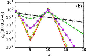
Figure 6: Concentrations $c_{k}$ of oligomers versus their length $k$ probed at the time $1000{\mathscr{T}}-0$ after a thousand serial transfers with fixed parameters (a) ${\mathscr{T}}=1$ and (b) ${\mathscr{T}}=0.1$ and for various values of $f$. Symbols correspond to $f=0.01$ (downward red triangles), $f=0.1$ (yellow diamonds), $f=0.5$ (magenta squares), $f=0.9$ (green stars), and black crosses represent the equilibrium distribution.

In order to test more precisely the convergence towards the CSTR dynamics, we have varied in Fig. 7 the parameters $(f,{\mathscr{T}})$ while keeping the residence time $\tau_{\rm eff}=\tau$ constant either at the value 1 or 0.1. The length distributions of the oligomers have been observed at the time $1000{\mathscr{T}}-0$. These plots indeed confirm that, in this system, a convergence towards the CSTR is obtained when $f\to 1$, which is equivalent to ${\mathscr{T}}\to 0$ since the residence time $\tau$ is kept constant.

In general, the state of the reactor following serial transfers with arbitrary parameters $(f,{\mathscr{T}})$ can differ substantially from the predictions of the CSTR. However, if the parameters $(f,{\mathscr{T}})$ are chosen according to Eq. (55) and the time of observation is not too long, as shown in Fig. 7, the behavior resulting from serial transfers can be quite close to that observed by the CSTR dynamics even when the parameter $f$ is varied in a large range from 0.001 to 0.99.

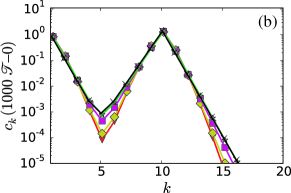
Figure 7: Concentrations $c_{k}$ of oligomers versus their length $k$ probed at the time $1000{\mathscr{T}}-0$ after a thousand serial transfers corresponding to varying $({\mathscr{T}},f)$ parameters at fixed residence time (a) $\tau_{\rm eff}=1$ or (b) $\tau_{\rm eff}=0.1$. Symbols correspond to $f=0.01$ (downward red triangles), $f=0.1$ (yellow diamonds), $f=0.5$ (magenta squares), $f=0.9$ (green stars), but now black crosses represent the length distribution predicted by the CSTR dynamics.

IV Conclusion

In this paper, we have made a comparative study of the kinetics and thermodynamics of open reactors (CSTR) with that of serial transfers between closed reactors. For a given choice of a chemical network and injected species, both the CSTR and the serial transfer dynamics admit a steady state. This implies that both systems will reach comparable composition on long times and also that the same cycles can be used to characterize the steady state of both systems. However, their dynamics can differ substantially. Only in the limit where the time interval between serial transfers tends to zero for a fixed residence time, the two dynamics are strictly equivalent.

We have also compared the properties of reaction networks in chemostatted systemsPolettini and Esposito (2014); Rao and Esposito (2016) with those in a CSTR. In contrast to chemostatted systems, the concentrations remain bounded in a CSTR. In a CSTR, there is no remaining conserved quantity and new cycles involving the exterior of the CSTR appear in addition to the cycles of the the closed reactor network. Similar results hold for the serial transfer dynamics.

This study was motivated by molecular evolution experiments which use serial transfers in the context of research on the origins of life.Vaidya et al. (2012) Besides chemical evolution by serial transfers, experiments in this field also use a dry-wet (or day-night) cycling protocol as a means of inducing an evolution in the composition of the system.Segré et al. (2000); Tkachenko and Maslov (2015); Forsythe et al. (2017) Many other cycling protocols are possible. In particular, cycles driven by thermal convectionMast et al. (2013) and cycles of activation-deactivation or of compartmentalization-decompartmentalization of specific speciesMatsumura et al. (2016) are being considered. We believe that the framework presented here could be extended to cover these cases provided the molecular interactions between the various species can be modeled.

Cycling protocols are often explored in the literature in order to explain how a population of sufficiently long chains can be self-sustained and show emergent properties, an important issue for the research on the origins of life. Our example of polymerization with mass exchange indicates that a population of polymers with a non-exponential distribution can be maintained in an open reactor if the residence time is not too long, thus solving the first issue. The second issue regarding the emergence of new properties is clearly more complex, but the framework used here allows at least to identify emergent cycles of the chemical network, which should capture important features of the emergent properties we are after.

Appendix A Analysis of the mass-exchange model

In order to determine the stationary concentrations of the mass-exchange model in the CSTR, we take the explicit form of the kinetic equations (41) with injection of monomers and oligomers of length $l$:Rao et al. (2015)

$$\frac{dc_{k}}{dt}=\kappa c(c_{k+1}-2c_{k}+c_{k-1})+\kappa c_{1}(c_{k}-c_{k-1})-\frac{1}{\tau}\,c_{k}\,,$$ (65)

for $1<k<l$ and $l<k$,

$$\frac{dc_{1}}{dt}=\kappa c(c_{2}-c_{1})+\kappa c_{1}^{2}+\frac{1}{\tau}(c_{1,0}-c_{1})\,,$$ (66)

and

$$\frac{dc_{l}}{dt} = \kappa c(c_{l+1}-2c_{l}+c_{l-1})+\kappa c_{1}(c_{l}-c_{l-1})$$ (67)

$$\qquad\qquad\qquad\qquad\quad\ +\frac{1}{\tau}(c_{l,0}-c_{1})\,,$$

where $c=\sum_{k=1}^{\infty}c_{k}$ is the sum of all the concentrations. Under the conditions of stationarity, this sum has reached its asymptotic value $c=c_{1,0}+c_{l,0}$, while the concentrations no longer depend on time: $dc_{k}/dt=0$. Under such conditions, Eqs. (65)-(67) form a set of linear equations for the concentrations $\{c_{k}\}_{k=1}^{\infty}$. The stationary solution is thus given by

$$c_{k,{\rm st}}=\left\{\begin{array}[]{ll}A\,\Lambda_{+}^{k}+B\,\Lambda_{-}^{k}\,,&\qquad\mbox{for}\quad 1\leq k\leq l\,,\\ C\,\Lambda_{-}^{k}\,,&\qquad\mbox{for}\quad l\leq k\,,\end{array}\right.$$ (68)

in terms of the roots of the characteristic polynomial:

$$\Lambda^{2}+\left(\frac{c_{1}}{c}-2-\frac{1}{c\kappa\tau}\right)\Lambda+1-\frac{c_{1}}{c}=0$$ (69)

with $\Lambda_{-}<1$.

If $\tau=\infty$, we recover the equilibrium exponential distribution (49) satisfying the conditions of detailed balance. In this case, the roots of Eq. (69) are $\Lambda_{+}=1$ and $\Lambda_{-}=1-c_{1}/c$. The normalizable distribution is thus given by $c_{k}=C\Lambda_{-}^{k}$ for $k\geq 1$, so that $C=cc_{1}/(c-c_{1})$. If $\tau=\infty$, the reactor is closed so that the quantities $c=\sum_{k=1}^{\infty}c_{k}$ and $M=\sum_{k=1}^{\infty}kc_{k}$ are invariant and they keep their initial values $c(0)=c$ and $M(0)=c^{2}/c_{1}$, hence the equilibrium distribution (49).

If $\tau$ is finite, the tail of the nonequilibrium distribution is still exponential, but the decay factor $\Lambda_{-}<1$ takes a different value than at equilibrium. If $\tau$ is large enough, the decay factor is approximately given by

$$\Lambda_{-}\simeq 1-\frac{c_{1}(\infty)}{c(\infty)}+O(\tau^{-1})\,,$$ (70)

and $c_{1}(\infty)=c(\infty)^{2}/M(\infty)+O(\tau^{-1})$. In this limit, the stationary distribution at large but finite values of the residence time is given by

$$c_{k,{\rm st}}\simeq\frac{c(\infty)^{2}}{M(\infty)}\left[1-\frac{c(\infty)}{M(\infty)}\right]^{k-1},\qquad\mbox{if}\quad c(\infty)\kappa\tau\gg 1\,.$$ (71)

However, the sum of all the concentrations is no longer a conserved quantity in the open reactor where it converges towards its injection value: $c(\infty)=c_{0}=c_{1,0}+c_{l,0}$. In the example of Fig. 4, the injection values of the two conserved quantities are respectively equal to $c(\infty)=c_{0}=3$ and $M(\infty)=M_{0}=21$, although their initial values are $c(0)=0.75331$ and $M(0)=0.9119$. This explains the observation in Fig. 4 that the distribution is decreasing more slowly as $c_{k,{\rm st}}\simeq 0.5\times(6/7)^{k}\simeq 0.5\times 0.857^{k}$ if $\tau=1000$ in the open reactor, than in the closed reactor if $\tau=\infty$.

If $\tau$ is small enough, the distribution becomes bimodal with two peaks at $c_{1,{\rm st}}\simeq c_{1,0}$ and $c_{l,{\rm st}}\simeq c_{l,0}$. In this limit, the tail of the distribution behaves as $c_{k}\simeq c_{l,0}\Lambda_{-}^{k-l}$ for $k\geq l$ with $\Lambda_{-}\simeq c_{l,0}\kappa\tau+O[(\kappa\tau)^{2}]$, so that the decay can be faster than at equilibrium, as seen in Fig. 4.

References

- Vaidya et al. (2012) N. Vaidya, M. L. Manapat, I. A. Chen, R. Xulvi-Brunet, E. J. Hayden, and N. Lehman, Nature 491, 72 (2012).
- Forsythe et al. (2017) J. G. Forsythe, A. S. Petrov, W. C. Millar, S.-S. Yu, R. Krishnamurthy, M. A. Grover, N. V. Hud, and F. M. Fernandez, Proc. Natl. Acad. Sci. U.S.A. 114, E7652 (2017).
- Eigen (1971) M. Eigen, Naturwissenschaften 58, 465 (1971).
- Eigen and Schuster (1977) M. Eigen and P. Schuster, Naturwissenschaften 64, 541 (1977).
- Eigen and Schuster (1978a) M. Eigen and P. Schuster, Naturwissenschaften 65, 7 (1978a).
- Eigen and Schuster (1978b) M. Eigen and P. Schuster, Naturwissenschaften 65, 341 (1978b).
- Eigen (1993) M. Eigen, Steps towards Life: A Perspective on Evolution (Oxford University Press, Oxford, 1993).
- Kauffman (1993) S. A. Kauffman, The Origins of Order: Self-Organization and Selection in Evolution, edited by O. U. P. Inc. (Oxford University Press, 1993).
- Segré et al. (2000) D. Segré, D. Ben-Eli, and D. Lancet, Proc. Natl. Acad. Sci. U.S.A. 97, 4112 (2000).
- Lincoln and Joyce (2009) T. A. Lincoln and G. F. Joyce, Science 323, 1229 (2009).
- Matsumura et al. (2016) S. Matsumura, Á. Kun, M. Ryckelynck, F. Coldren, A. Szilágyi, F. Jossinet, C. Rick, P. Nghe, E. Szathmáry, and A. D. Griffiths, Science 354, 1293 (2016).
- Zwaag and Meijer (2015) D. v. d. Zwaag and E. W. Meijer, Science 349, 1056 (2015).
- Zeravcic et al. (2017) Z. Zeravcic, V. N. Manoharan, and M. P. Brenner, Rev. Mod. Phys. 89, 031001 (2017).
- Agresti et al. (2010) J. J. Agresti, E. Antipov, A. R. Abate, K. Ahn, A. C. Rowat, J.-C. Baret, M. Marquez, A. M. Klibanov, A. D. Griffiths, and D. A. Weitz, Proc. Natl. Acad. Sci. U.S.A. 107, 4004 (2010).
- Arnold and Moore (1997) F. Arnold and J. Moore, Adv. Biochem. Eng. Biotechnol. 58, 1 (1997).
- Hill (1989) T. L. Hill, Free Energy Transduction and Biochemical Cycle Kinetics (Springer, 1989).
- Padinhateeri et al. (2012) R. Padinhateeri, A. Kolomeisky, and D. Lacoste, Biophys. J. 102, 1274 (2012).
- Jégou and Romet-Lemonne (2016) A. Jégou and G. Romet-Lemonne, Biophysical Journal, Biophys. J. 110, 2138 (2016).
- Brangwynne et al. (2009) C. P. Brangwynne, C. R. Eckmann, D. S. Courson, A. Rybarska, C. Hoege, J. Gharakhani, F. Jülicher, and A. A. Hyman, Science 324, 1729 (2009).
- Zwicker et al. (2017) D. Zwicker, R. Seyboldt, C. A. Weber, A. A. Hyman, and F. Jülicher, Nat. Phys. 13, 408 (2017).
- Marchetti et al. (2013) M. C. Marchetti, J. F. Joanny, S. Ramaswamy, T. B. Liverpool, J. Prost, M. Rao, and R. A. Simha, Rev. Mod. Phys. 85, 1143 (2013).
- Nicolis and Prigogine (1977) G. Nicolis and I. Prigogine, Self-Organization in Nonequilibrium Systems: From Dissipative Structures to Order through Fluctuations (Wiley, New York, 1977).
- Prigogine (1967) I. Prigogine, Introduction to Thermodynamics of Irreversible Processes (Wiley, New York, 1967).
- de Groot and Mazur (1984) S. R. de Groot and P. Mazur, Nonequilibrium Thermodynamics (Dover, New York, 1984).
- Polettini and Esposito (2014) M. Polettini and M. Esposito, J. Chem. Phys. 141, 024117 (2014).
- Rao and Esposito (2016) R. Rao and M. Esposito, Phys. Rev. X 6, 041064 (2016).
- Lahiri et al. (2015) S. Lahiri, Y. Wang, M. Esposito, and D. Lacoste, New J. Phys. 17, 085008 (2015).
- Rao et al. (2015) R. Rao, D. Lacoste, and M. Esposito, J. Chem. Phys. 143, 244903 (2015).
- Blokhuis and Lacoste (2017) A. Blokhuis and D. Lacoste, J. Chem. Phys. 147, 094905 (2017).
- Aris (1989) R. Aris, Elementary Chemical Reactor Analysis (Dover, Mineola NY, 1989).
- Bergé et al. (1984) P. Bergé, Y. Pomeau, and C. Vidal, L’ordre dans le chaos (Hermann, Paris, 1984).
- Vidal and Lemarchand (1988) C. Vidal and H. Lemarchand, La réaction créatrice: Dynamique des systèmes chimiques (Hermann, Paris, 1988).
- Nicolis (1995) G. Nicolis, Introduction to nonlinear science (Cambridge University Press, Cambridge UK, 1995).
- Epstein and Pojman (1998) I. R. Epstein and J. A. Pojman, An Introduction to Nonlinear Chemical Dynamics (Oxford University Press, New York, 1998).
- Scott (1991) S. K. Scott, Chemical Chaos (Clarendon Press, Oxford, 1991).
- Salman et al. (2012) H. Salman, N. Brenner, C.-k. Tung, N. Elyahu, E. Stolovicki, L. Moore, A. Libchaber, and E. Braun, Phys. Rev. Lett. 108, 238105 (2012).
- Tkachenko and Maslov (2015) A. V. Tkachenko and S. Maslov, J. Chem. Phys. 143, 045102 (2015).
- Mast et al. (2013) C. B. Mast, S. Schink, U. Gerland, and D. Braun, Proc. Natl. Acad. Sci. U.S.A. 110, 8030 (2013).