On the utility of Metropolis-Hastings with asymmetric acceptance ratio

Abstract

The Metropolis–Hastings algorithm allows one to sample asymptotically from any probability distribution $\pi$ admitting a density with respect to a reference measure, also denoted $\pi$ here, which can be evaluated pointwise up to a normalising constant. There has been recently much work devoted to the development of variants of the Metropolis–Hastings update which can handle scenarios where such an evaluation is impossible, and yet are guaranteed to sample from $\pi$ asymptotically. The most popular approach to have emerged is arguably the pseudo-marginal Metropolis–Hastings algorithm which substitutes an unbiased estimate of an unnormalised version of $\pi$ for $\pi$ (Lin et al., 2000; Beaumont, 2003; Andrieu and Roberts, 2009). Alternative pseudo-marginal algorithms relying instead on unbiased estimates of the Metropolis–Hastings acceptance ratio have also been proposed (Neal, 2004; Murray et al., 2006; Nicholls et al., 2012). These algorithms can have better properties than standard pseudo-marginal algorithms. Convergence properties of both classes of algorithms are known to depend on the variability (in the sense of the convex order) of the estimators involved (Andrieu and Vihola, 2014), and reduced variability is guaranteed to decrease the asymptotic variance of ergodic averages and will shorten the “burn-in” period, or convergence to equilibrium, in most scenarios of interest. A simple approach to reduce variability, amenable to parallel computations, consists of averaging independent estimators. However, while averaging estimators of $\pi$ in a pseudo-marginal algorithm retains the guarantee of sampling from $\pi$ asymptotically, naive averaging of acceptance ratio estimates breaks detailed balance, leading to incorrect results. We propose an original methodology which allows for a correct implementation of this idea. We establish theoretical properties which parallel those available for standard pseudo-marginal algorithms and discussed above. We demonstrate the interest of the approach on various inference problems involving doubly intractable distributions, latent variable models, model selection, and state-space models. In particular we show that convergence to equilibrium can be significantly shortened, therefore offering the possibility to reduce a user’s waiting time in a generic fashion when a parallel computing architecture is available.

^∗School of Mathematics, University of Bristol, U.K.
^†Department of Statistics, University of Oxford, U.K.
⁺Faculty of Engineering and Natural Sciences, Sabancı University, Turkey.
^◆ENSAE, France.

Keywords: Annealed Importance Sampling; Doubly intractable distributions; Intractable likelihood; Markov chain Monte Carlo; Reversible jump Monte Carlo; Sequential Monte Carlo; State-space models.

1 Introduction

Suppose we are interested in sampling from a given probability distribution $\pi$ on some measurable space $(\mathsf{X},\mathcal{X})$. When it is impossible or too difficult to generate perfect samples from $\pi$, one practical resource is to use a Markov chain Monte Carlo (MCMC) algorithm which generates an ergodic Markov chain $\{X_{n},n\geq 0\}$ whose invariant distribution is $\pi$. Among MCMC methods, the Metropolis–Hastings (MH) algorithm plays a central rôle. The MH update proceeds as follows: given $X_{n}=x$ and a Markov transition kernel $q\big{(}x,\cdot\big{)}$ on $(\mathsf{X},\mathcal{X})$, we propose $y\sim q(x,\cdot)$ and set $X_{n+1}=y$ with probability $\alpha(x,y):=\min\left\{1,r(x,y)\right\}$, where

$$r(x,y):=\frac{\pi({\rm d}y)q(y,{\rm d}x)}{\pi({\rm d}x)q(x,{\rm d}y)}$$ (1)

for $(x,y)\in\mathsf{S}\subset\mathsf{X}^{2}$ (see Appendix A for a definition of $\mathsf{S}$) is a well defined Radon–Nikodym derivative, and $r(x,y)=0$ otherwise. When the proposed value $y$ is rejected, we set $X_{n+1}=x$. We will refer to $r(x,y)$ as the acceptance ratio. The transition kernel of the Markov chain $\{X_{n},n\geq 0\}$ generated with the MH algorithm with proposal kernel $q(\cdot,\cdot)$ is

$$P(x,{\rm d}y)=q(x,{\rm d}y)\alpha(x,y)+\rho(x)\delta_{x}({\rm d}y),\quad x\in\mathsf{X},$$ (2)

where $\rho(x)$ is the probability of rejecting a proposed sample when $X_{n}=x$,

$$\rho(x):=1-\int_{\mathsf{X}}\alpha(x,y)Q(x,{\rm d}y)$$

and $\delta_{x}(\cdot)$ is the Dirac measure centred at $x$. Expectations of functions, say $f$, with respect to $\pi$ can be estimated with $S_{M}:=M^{-1}\sum_{n=1}^{M}f(X_{n})$ for $M\in\mathbb{N}$, which is consistent under mild assumptions.

Being able to evaluate the acceptance ratio $r(x,y)$ is obviously central to implementing the MH algorithm in practice. Recently, there has been much interest in expanding the scope of the MH algorithm to situations where this acceptance ratio is intractable, that is, impossible or very expensive to compute. A canonical example of intractability is when $\pi$ can be written as the marginal of a given joint probability distribution for $x$ and some latent variable $z$. A classical way of addressing this problem consists of running an MCMC targeting the joint distribution, which may however become very inefficient in situations where the size of the latent variable is high–this is for example the case for general state-space models. In what follows, we will briefly review some more effective ways of tackling this problem. To that purpose we will use the following simple running example to illustrate various methods. This example has the advantage that its setup is relatively simple and of clear practical relevance. We postpone developments for much more complicated setups to Sections 4 and 5.

Example 1 (Inference with doubly intractable models).

In this scenario the likelihood function of the unknown parameter $\theta\in\Theta$ for the dataset $\mathfrak{y}\in\mathsf{Y}$, $\ell_{\theta}(\mathfrak{y})$, is only known up to a normalising constant, that is

$$\ell_{\theta}(\mathfrak{y})=\frac{g_{\theta}(\mathfrak{y})}{C_{\theta}},$$

where $C_{\theta}$ is unknown, while $g_{\theta}(\mathfrak{y})$ can be evaluated pointwise for any value of $\theta\in\Theta$. In a Bayesian framework, for a prior density $\eta(\theta)$, we are interested in the posterior density $\pi(\theta)$, with respect to some measure, given by

$$\pi(\theta)\propto\eta(\theta)\ell_{\theta}(\mathfrak{y}).$$

With $x=\theta,y=\theta^{\prime}$ in (1), the resulting acceptance ratio of the MH algorithm associated to a proposal density $q(\theta,\theta^{\prime})$ is

$$r(\theta,\theta^{\prime})=\frac{q(\theta^{\prime},\theta)}{q(\theta,\theta^{\prime})}\frac{\eta(\theta^{\prime})}{\eta(\theta)}\frac{g_{\theta^{\prime}}(\mathfrak{y})}{g_{\theta}(\mathfrak{y})}\frac{C_{\theta}}{C_{\theta^{\prime}}},$$ (3)

which cannot be calculated because of the unknown ratio $C_{\theta}/C_{\theta^{\prime}}$. While the likelihood function may be intractable, sampling artificial datasets $\mathfrak{z}\sim\ell_{\theta}(\cdot)$ may be possible for any $\theta\in\Theta$, and sometimes computationally cheap. We will describe two known approaches which exploit and expand this property in order to design Markov kernels preserving $\pi(\theta)$ as invariant density.

1.1 Estimating the target density

Assume for simplicity that $\pi$ has a probability density with respect to some $\sigma$-finite measure. We will abuse notation slightly by using $\pi$ for both the probability distribution and its density. A powerful, yet simple, method to tackle intractability which has recently attracted substantial interest consists of replacing the value of $\pi(x)$ with a non-negative random estimator $\hat{\pi}(x)$ whenever it is required in the implementation of the MH algorithm above. If $\mathbb{E}[\hat{\pi}(x)]=C\pi(x)$ for all $x\in\mathsf{X}$ and a constant $C>0$, a property we refer somewhat abusively as unbiasedness, this strategy turns out to lead to exact algorithms, that is sampling from $\pi$ is guaranteed at equilibrium under very mild assumptions on $\hat{\pi}(x)$. This approach leads to so called pseudo-marginal algorithms (Andrieu and Roberts, 2009). However, for reasons which will become clearer later, we refer from now on to these techniques as Pseudo-Marginal Target (PMT) algorithms.

Example 2 (Example 1, ctd).

Let $h_{\mathfrak{y}}:\mathsf{Y}\rightarrow[0,\infty)$ be an integrable non-negative function of integral equal to $1$. For a given $\theta$, an unbiased estimate of $\pi(\theta)$ can be obtained via importance sampling whenever the support of $g_{\theta}$ includes that of $h_{\mathfrak{y}}$:

$$\hat{\pi}^{N}(\theta)\propto\eta(\theta)g_{\theta}(\mathfrak{y})\left\{\frac{1}{N}\sum_{i=1}^{N}\frac{h_{\mathfrak{y}}(\mathfrak{z}^{(i)})}{g_{\theta}(\mathfrak{z}^{(i)})}\right\},\quad\mathfrak{z}^{(i)}\overset{{\rm iid}}{\sim}\ell_{\theta}(\cdot),\quad i=1,\ldots,N,$$ (4)

since the normalised sum is an unbiased estimator of $1/C_{\theta}$. The auxiliary variable method of Møller et al. (2006) corresponds to $N=1$. An interesting feature of this approach is that $N$ is a free parameter of the algorithm which reduces the variability of this estimator. It is shown in Andrieu and Vihola (2014) that increasing $N$ in a PMT algorithm always reduces the asymptotic variance of averages using this chain. This is particularly interesting in a parallel computing environment, but also serial for some models. We illustrate this numerically on a simple Ising model (see details in Section 3.3) for a $20\times 20$ lattice and $h_{\mathfrak{y}}(\mathfrak{z})=g_{\hat{\theta}}\big{(}\mathfrak{z}\big{)}$, where $\hat{\theta}$ is an approximation of the maximum likelihood estimator of $\theta$ for the data $\mathfrak{y}$. In Figure 1 we report the estimated integrated auto-covariance (IAC) for the identity, that is $\lim_{M\rightarrow\infty}M\mathsf{\mathbb{\mathsf{var}}}\big{(}S_{M}\big{)}/\mathbb{\mathsf{var}}_{\pi}(f)$ for the function $f(\theta)=\theta$, as a function of $N$ and values of $\hat{\theta}$. The results are highly dependent on the value of $\hat{\theta}$, but adjusting $N$ allows one to compensate for a wrong choice of this parameter. This is important in practice since for more complicated scenarios obtaining a good approximation of the maximum likelihood estimator of $\theta$ may be difficult.

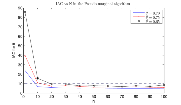
Figure 1: IAC of the algorithm as a function of $N$.

1.2 Estimating the acceptance ratio

One can in fact push the idea of replacing algebraic expressions with estimators further. Instead of approximating the numerator and denominator of the acceptance ratio $r(x,y)$ independently, it is indeed possible to use directly estimators of the acceptance ratio $r(x,y)$ and still obtain algorithms guaranteed to sample from $\pi$ at equilibrium. We will refer to these algorithms as Pseudo-Marginal Ratio (PMR) algorithms. A general framework is described in Andrieu and Vihola (2014) as well as in Section 2.1, but this idea has appeared earlier in various forms in the literature, see e.g. Nicholls et al. (2012) and the references therein. An interesting feature of PMR algorithms is that we estimate the ratio $r(x,y)$ afresh whenever it is required. On the contrary, in a PMT framework, if the estimate $\hat{\pi}(x)/C$ of the current state significantly overestimates $\pi(x)$, this results in poor performance as the algorithm will typically reject many transitions away from $x$ as the same estimate of $\pi(x)$ is used until a proposal is accepted. In the following continuation of Example 1, we present a particular case of this PMR idea proposed by Murray et al. (2006).

Example 3 (Example 1, ctd).

The exchange algorithm of Murray et al. (2006) is motivated by the realisation that while for $\mathfrak{z}\sim\ell_{\theta^{\prime}}(\cdot)$ and any $\mathfrak{y}\in\mathsf{Y}$, $h_{\mathfrak{y}}(\mathfrak{z})/g_{\theta^{\prime}}(\mathfrak{z})$ is an unbiased estimator of $1/C_{\theta^{\prime}}$, the particular choice $h_{\mathfrak{y}}(\mathfrak{z})=g_{\theta}(\mathfrak{z})$ leads to an unbiased estimator $g_{\theta}(\mathfrak{z})/g_{\theta^{\prime}}(\mathfrak{z})$ of $C_{\theta}/C_{\theta^{\prime}}$. We can expect this estimator to have a reasonable variance when $\theta$ and $\theta^{\prime}$ are close if $\theta\mapsto g_{\theta}(\mathfrak{z})$ satisfies some form of continuity. This suggests the following algorithm. Given $\theta\in\Theta$, sample $\theta^{\prime}\sim q(\theta,\cdot)$, then $\mathfrak{z}\sim\ell_{\theta^{\prime}}(\cdot)$ and use the acceptance ratio

$$\frac{q(\theta^{\prime},\theta)}{q(\theta,\theta^{\prime})}\frac{\eta(\theta^{\prime})}{\eta(\theta)}\frac{g_{\theta^{\prime}}(\mathfrak{y})}{g_{\theta}(\mathfrak{y})}\frac{g_{\theta}(\mathfrak{z})}{g_{\theta^{\prime}}(\mathfrak{z})},$$ (5)

which is an unbiased estimator of the acceptance ratio in (3). The remarkable property of this algorithm is that it admits $\pi(\theta)$ as an invariant distribution and hence, under mild exploration related assumptions, it is guaranteed to produce samples asymptotically distributed according to $\pi$.

1.3 Contribution

As for PMT algorithms, it is natural to ask whether it is possible to further improve the performance of PMR algorithms by reducing the variability of the acceptance ratio estimator by averaging a number of such estimators, while preserving the target distribution $\pi$ invariant. We shall see that, unfortunately, such naïve averaging approach does not work for the PMR methods currently available as it breaks the reversibility of the kernels with respect to $\pi$.

A contribution of the present paper is the introduction of a novel class of PMR algorithms which can exploit acceptance ratio estimators obtained through averaging and sample from $\pi$ at equilibrium. These algorithms described in Section 2 naturally lend themselves to parallel computations as independent ratio estimators can be computed in parallel at each iteration. In this respect, our methodology contributes to the emerging literature on the use of parallel processing units, such as Graphics Processing Units (GPUs) or multicore chips for scientific computation Lee et al. (2010); Suchard et al. (2010). We show that this generic procedure is guaranteed to decrease the asymptotic variance of ergodic averages as the number of independent ratios $N$ one averages increases and that the burn-in period will be reduced in most scenarios. The latter is particularly relevant since exact and generic methods to achieve this are scarce (Sohn, 1995), in contrast with variance reduction techniques for which better embarrassingly parallel solutions (Sherlock et al., 2017; Bornn et al., 2017) and/or post-processing methods are available (Delmas and Jourdain, 2009; Dellaportas and Kontoyiannis, 2012). We demonstrate experimentally its performance gain for the exchange algorithm.

This new class of PMR algorithms can be understood as being a particular instance of a more general principle which we exploit further in this paper, beyond the above example. Let $Q_{1},Q_{2}\colon\mathsf{X}\times\mathcal{X}\rightarrow[0,1]$ be a pair of kernels such that the following Radon-Nikodym derivative

$$r_{1}(x,y):=\frac{\pi({\rm d}y)Q_{2}(y,{\rm d}x)}{\pi({\rm d}x)Q_{1}(x,{\rm d}y)}$$

is well defined for $(x,y)$ on some symmetric set $\mathsf{S}$ and set $r_{1}(x,y)=0$ otherwise. This can be thought of as an asymmetric version of the standard MH acceptance ratio (1) and naturally leads to two questions.

1. Assuming that sampling from $Q_{1}(x,\cdot)$ and $Q_{2}(x,\cdot)$ for any $x\in\mathsf{X}$ is feasible and that $r_{1}(x,y)$ is tractable, can one design a correct MCMC algorithm for $\pi$ that involves simulating from $Q_{1}(x,\cdot)$ and $Q_{2}(x,\cdot)$ and evaluating $r_{1}(x,y)$ ?

2. Assuming the answer to the above is positive, can this additional degree of freedom be beneficial in order to design correct MCMC algorithms with practically appealing features e.g. accelerated convergence?

The answer to the first question is unsurprisingly yes, and we will refer to the corresponding class of algorithms as MH with Asymmetric Acceptance Ratio (MHAAR). MHAAR has already been exploited in some specific contexts (Tjelmeland and Eidsvik, 2004; Andrieu and Thoms, 2008), but its best known application certainly remains the reversible jump MCMC methodology of Green (1995). However the way we take advantage of this additional flexibility seems completely novel. We also note, as detailed in our discussion in Section 6, that such asymmetric acceptance ratios are also at the heart of non-reversible MCMC algorithms which have recently attracted renewed interest in the Physics and Statistical communities (Gustafson, 1998; Turitsyn et al., 2011). In Appendix A, we describe and justify a slightly more general framework to the above which ensures reversibility with respect to $\pi$. The answer to the second question is the object of this paper, and averaging acceptance ratios as suggested earlier is one such application.

In Section 3 we further investigate the doubly intractable scenario by incorporating the Annealed Importance Sampling (AIS) mechanism (Neal, 2001; Murray et al., 2006) in MHAAR, and explore numerically the performance of MHAAR with AIS on an Ising model.

In Section 4 we expand the class of problems our methodology can address by considering latent variable models. This leads to important extensions of the original AIS within MH algorithm proposed in Neal (2004). We demonstrate the efficiency of our MHAAR-based approach by recasting the popular reversible jump MCMC (RJ-MCMC) methodology as a particular case of our framework and illustrate the computational benefits of our novel algorithm in this context on the Poisson change-point model in Green (1995).

In Section 5, we show how MHAAR can be advantageous in the context of inference in state-space models when it is utilised with sequential Monte Carlo (SMC) algorithms. In particular, we expand the scope of particle MCMC algorithms (Andrieu et al., 2010) and show novel ways of using multiple or all possible paths from backward sampling of conditional SMC (cSMC) to estimate the marginal acceptance ratio.

In Section 6, we provide some discussion and two interesting extensions of MHAAR. Specifically, in Section 6.1 we discuss an SMC-based generalisation of our algorithms involving AIS. Furthermore, in Section 6.2 we provide a new insight to non-reversible versions of MH algorithms that is relevant to our setting. We briefly demonstrate how non-reversible versions of our algorithms can be obtained with a small modification so that one can benefit both from non-reversibility and the ability to average acceptance ratio estimators.

Some of the proofs of the validity of our algorithms as well as additional discussion on the generalisation of the methods can found in the Appendices.

2 PMR algorithms using averaged acceptance ratio estimators

2.1 PMR algorithms

We introduce here generic PMR algorithms, that is MH algorithms relying on an estimator of the acceptance ratio. We then show that in their standard form these algorithms cannot use an estimator of this ratio obtained through averaging independent estimators. A slightly more general framework is provided in Nicholls et al. (2012), while a more abstract description is provided in Andrieu and Vihola (2014). To that purpose we introduce a $(\mathsf{U},\mathcal{U})$-valued auxiliary variable $u$ (we use small letters for random variables and realisations throughout) and let $\varphi:\mathsf{U}\rightarrow\mathsf{U}$ be a measurable involution, that is $\varphi=\varphi^{-1}$. Then we introduce a pair of families of proposal distributions $\{Q_{1}(x,\cdot),x\in\mathsf{X}\}$ , $\{Q_{2}(x,\cdot),x\in\mathsf{X}\}$ on $(\mathsf{X}\times\mathsf{U},\mathcal{X}\times\mathcal{U})$, where

$$Q_{1}\big{(}x,{\rm d}(y,u)\big{)}:=q(x,{\rm d}y)Q_{x,y}({\rm d}u)$$ (6)

with $Q_{x,y}(\cdot)$ denoting the conditional distribution of $u$ given $x,y\in\mathsf{X}$, and

$$Q_{2}\big{(}x,{\rm d}(y,u)\big{)}:=q(x,{\rm d}y)\bar{Q}_{x,y}({\rm d}u),$$ (7)

where, for any $A\in\mathcal{U}$ we have

$$\bar{Q}_{x,y}\big{(}A\big{)}:=Q_{x,y}\big{(}\varphi(A)\big{)}.$$ (8)

which means that in order to sample $u\sim\bar{Q}_{x.y}(\cdot)$, one can sample $\bar{u}\sim Q_{x,y}(\cdot)$ and set $u=\varphi(\bar{u})$. PMR algorithms are defined by the following transition kernel

$$\mathring{P}(x,{\rm d}y)=\int_{\mathsf{U}}Q_{1}\big{(}x,{\rm d}(y,u)\big{)}\min\{1,\mathring{r}_{u}(x,y)\}+\mathring{\rho}(x)\delta_{x}({\rm d}y),$$ (9)

where the acceptance ratio is equal, for $(x,y,u)\in\mathring{\mathsf{S}}$ and $\mathring{\mathsf{S}}$ defined similarly to (47), to

$$\mathring{r}_{u}(x,y) :=\frac{\pi({\rm d}y)Q_{2}\big{(}y,{\rm d}(x,u)\big{)}}{\pi(dx)Q_{1}\big{(}x,{\rm d}(y,u)\big{)}}$$ (10)

$$=r(x,y)\frac{\bar{Q}_{y,x}({\rm d}u)}{Q_{x,y}({\rm d}u)},$$

and to $1$ otherwise. It is clear from (10) that the acceptance ratio $\mathring{r}_{u}(x,y)$ is an unbiased estimator of the standard MH acceptance $r(x,y)$, i.e.

$$\int_{\mathsf{U}}\mathring{r}_{u}(x,y)Q_{x,y}({\rm d}u)=r(x,y).$$ (11)

Due to the particular form of symmetry between $Q_{1}$ and $Q_{2}$ imposed by (8), $\mathring{P}$ is reversible with respect to $\pi$ by considering detailed balance for fixed $u\in\mathsf{U}$; see Theorem 5 in Appendix A.

As long as PMR algorithms are concerned, we call $Q_{1}$ the proposal kernel of PMR and $Q_{2}$ its complementary kernel, owing to the way (9) is constructed. Motivation for this enumeration will be clear in Section 2.2, in particular by Remark 3.

Remark 1.

A cautionary remark is in order. When we substitute a non-negative unbiased estimator of $\pi$ for $\pi$ in the MH algorithm, the resulting PMT algorithm is $\pi-$invariant. However, if we substitute a positive unbiased estimator of $r(x,y)$ for $r(x,y)$ in the MH algorithm then the resulting transition kernel is not necessarily $\pi-$invariant. To establish that $\mathring{P}$ is $\pi-$invariant, we require our estimator to have the specific structure given in (10).

A particular instance of this algorithm was given earlier in the set-up of Example 1, where $x=\theta$, the random variable $u=\mathfrak{z}$ corresponds to a fictitious dataset used to estimate the ratio of normalising constants, and $\varphi(u)=u$. The need to consider more general transformations $\varphi$ will become apparent in Section 3.

This type of algorithms is motivated by the fact that while in some situations $r(x,y)$ cannot be computed, the introduction of the auxiliary variable $u$ makes the computation of $\mathring{r}_{u}(x,y)$ possible. However, this computational tractability comes at a price. Applying Jensen’s inequality to (11) shows that

$$\int_{\mathsf{U}}Q_{x,y}({\rm d}u)\min\{1,\mathring{r}_{u}(x,y)\}\leq\min\{1,r(x,y)\}.$$

Peskun’s result (Tierney, 1998) thus implies that the MCMC algorithm relying on $\mathring{P}$ is always inferior to that using $P$ for various performance measures (see Theorem 1 for details). As pointed out in Andrieu and Vihola (2014) reducing the variability of $\mathring{r}_{u}(x,y)$, for example in the sense of the convex order, for all $x,y\in\mathsf{X}^{2}$ will reduce the gap in the inequality above, resulting in improved performance. From the rightmost expression in (10) a possibility to reduce variability might be to change $Q_{x,y}\big{(}\cdot\big{)}$ (and possibly $u$) in such a way that $Q_{x,y}\simeq\bar{Q}_{y,x}$ for all $x,y\in\mathsf{X}$, but this is impossible in most practical scenarios. In contrast a natural idea consists of averaging ratios $\mathring{r}_{u^{(i)}}(x,y)$’s for, say, realisations $u^{(1)},\ldots,u^{(N)}\overset{{\rm iid}}{\sim}Q_{x,y}(\cdot)$ and use the acceptance ratio

$$\mathring{r}_{\mathfrak{u}}^{N}(x,y):=\frac{1}{N}\sum_{i=1}^{N}\mathring{r}_{u^{(i)}}(x,y),$$ (12)

where $\mathfrak{u}:=u^{(1:N)}=\big{(}u^{(1)},\ldots,u^{(N)}\big{)}\in\mathfrak{U}:=\mathsf{U}^{N}$–we drop the dependence on $N$ in order to alleviate notation whenever no ambiguity is possible. While this reduces the variance of the estimator of $r\big{(}x,y\big{)}$, this naïve modification of the acceptance rule of $\mathring{P}$ breaks detailed balance with respect to $\pi$. Indeed one can check that with $Q_{1}^{N}(x,{\rm d}(y,\mathfrak{u})):=q(x,{\rm d}y)\prod_{i=1}^{N}Q_{x,y}({\rm d}u^{(i)})$, $h:\mathsf{X}^{2}\rightarrow\mathbb{R}$ a bounded measurable function and using Fubini’s result,

$$\int_{\mathsf{X}\times\mathfrak{U}\times\mathsf{X}}\pi\big{(}{\rm d}x\big{)}Q_{1}^{N}\big{(}x,{\rm d}(y,{\rm\mathfrak{u})}\big{)}\min\{1,\mathring{r}_{\mathfrak{u}}^{N}(x,y)\}h\big{(}x,y\big{)}$$

$$\neq\int_{\mathsf{X}\times\mathfrak{U}\times\mathsf{X}}\pi\big{(}{\rm d}y\big{)}Q_{1}^{N}\big{(}y,{\rm d}(x,{\rm\mathfrak{u}})\big{)} \min\{1,\mathring{r}_{\mathfrak{u}}^{N}(y,x)\}h\big{(}x,y\big{)}$$

in general. This is best seen in a scenario where $\mathsf{X}$ and $\mathsf{U}$ are finite and $h(x,y)=\mathbb{I}\{x=a\}\mathbb{I}\{y=b\}$ for some $a,b\in\mathsf{X}$, and it can be shown that $\pi$ is not left invariant by the corresponding Markov transition probability.

2.2 MHAAR for averaging PMR estimators

We show here how MHAAR updates can be used in order to use the acceptance ratio in (12), while preserving $\pi-$reversibility. Our novel scheme is described in Algorithm 1. For $m\in\mathbb{N}$ and $w_{1},\ldots,w_{m}\in\mathbb{R}_{+}$ we let $\mathcal{P}\big{(}w_{1},\ldots,w_{m}\big{)}$ denote the probability distribution of the random variable $\omega$ on $[m]:=\{1,\ldots,m\}$ such that $\mathbb{P}(\omega=k)\propto w_{k}$.

1

Input: Current sample $X_{n}=x$

2

Output: New sample $X_{n+1}$

3

4Sample $y\sim q(x,\cdot)$ and $v\sim\mathcal{U}(0,1)$.

5 if $v\leq 1/2$ then

6      

7      Sample $u^{(1)},\ldots,u^{(N)}\overset{{\rm iid}}{\sim}Q_{x,y}(\cdot)$ and $k\sim\mathcal{P}\big{(}\mathring{r}_{u^{(1)}}\big{(}x,y\big{)},\ldots,\mathring{r}_{u^{(N)}}\big{(}x,y\big{)}\big{)}$.

8       Set $X_{n+1}=y$ with probability $\min\{1,\mathring{r}_{\mathfrak{u}}^{N}(x,y)\}$, otherwise set $X_{n+1}=x$.

9else

10      

11      Sample $k\sim\mathcal{U}\big{\{}1,\ldots,N\big{\}}$, $u^{(k)}\sim\bar{Q}_{x,y}(\cdot)$ and $u^{(1)},\ldots,u^{(k-1)},u^{(k+1)},\ldots,u^{(N)}\overset{{\rm iid}}{\sim}Q_{y,x}(\cdot)$

12       Set $X_{n+1}=y$ with probability $\min\{1,1/\mathring{r}_{\mathfrak{u}}^{N}(y,x)\}$, otherwise set $X_{n+1}=x$.

Algorithm 1 MHAAR for averaging PMR estimators

The unusual step in this update is the random choice between two sampling mechanisms for the auxiliary variables $u^{(1)},\ldots,u^{(N)}$ and the fact that depending on this choice either $\mathring{r}_{\mathfrak{u}}^{N}(x,y)$ or $1/\mathring{r}_{\mathfrak{u}}^{N}(y,x)$ is used. Apart from the reversible jump MCMC context (Green, 1995) and specific uses Tjelmeland and Eidsvik (2004); Andrieu and Thoms (2008), this type of asymmetric updates has rarely been used –see Appendix A.2 for an extensive discussion and from Section 4 on for other applications. The probability distributions corresponding to the two proposal mechanisms in Algorithm 1 are given by

$$Q_{1}^{N}\big{(}x,{\rm d}(y,\mathfrak{u},k)\big{)} :=q(x,{\rm d}y)\prod_{i=1}^{N}Q_{x,y}({\rm d}u^{(i)})\frac{\mathring{r}_{u^{(k)}}(x,y)}{\sum_{i=1}^{N}\mathring{r}_{u^{(i)}}(x,y)},$$

$$Q_{2}^{N}\big{(}x,{\rm d}(y,\mathfrak{u},k)\big{)} :=q(x,{\rm d}y)\frac{1}{N}\bar{Q}_{x,y}({\rm d}u^{(k)})\prod_{i=1,i\neq k}^{N}Q_{y,x}(\mathrm{d}u^{(i)}),$$

and the corresponding Markov transition kernel by

$$\mathring{P}^{N}(x,{\rm d}y):=\frac{1}{2}\left[\int_{\mathfrak{U}\times[N]}Q_{1}^{N}\big{(}x,{\rm d}(y,\mathfrak{u},k)\big{)}\min\left\{1,\mathring{r}_{\mathfrak{u}}^{N}(x,y)\right\}+\mathring{\rho}_{1}(x)\delta_{x}({\rm d}y)\right]$$

$$\quad\quad\quad\quad\quad\quad\quad+\frac{1}{2}\left[\int_{\mathfrak{U}\times[N]}Q_{2}^{N}\big{(}x,{\rm d}(y,\mathfrak{u},k)\big{)}\min\left\{1,1/\mathring{r}_{\mathfrak{u}}^{N}(y,x)\right\}+\mathring{\rho}_{2}(x)\delta_{x}({\rm d}y)\right],$$ (13)

where $\mathring{\rho}_{1}(x)$ and $\mathring{\rho}_{2}(x)$ are the rejection probabilities for each sampling mechanism. We establish the $\pi-$reversibility of $\mathring{P}^{N}$ in Theorem 1.

Remark 2.

It is necessary to include the variable $k$ in $Q_{1}^{N}$ and $Q_{2}^{N}$ to obtain tractable acceptance ratios validating the algorithm but, practically, its value is clearly redundant in Algorithm 1 and sampling $k$ is therefore not required.

Remark 3.

$Q_{1}^{N}$ and $Q_{2}^{N}$ reduce to $Q_{1}$ and $Q_{2}$ in (6) and (7) when $N=1$ in which case $k$ becomes redundant. This implies generality over PMR algorithms even for $N=1$ (although probably not a useful one), in the sense that in MHAAR one can also propose from $Q_{2}$.

Example 4 (Example 2, ctd).

As noticed in Nicholls et al. (2012), the exchange algorithm (Murray et al., 2006) can be recast as a PMR algorithm of the form $\mathring{P}$ given in (9) where $x=\theta,y=\theta^{\prime},u=\mathfrak{z}$, $\varphi(u)=u$ and $Q_{x,y}$ corresponds to $\ell_{\theta^{\prime}}$. Hence an extension of this algorithm using an averaged acceptance ratio estimator is given by Algorithm 1. Taking into account Remark 2, this takes the following form. Sample $\theta^{\prime}\sim q(\theta,\cdot)$, then with probability $1/2$ sample $u^{(1)},\ldots,u^{(N)}\overset{{\rm iid}}{\sim}\ell_{\theta^{\prime}}(\cdot)$ and compute

$$\mathring{r}_{\mathfrak{u}}^{N}(\theta,\theta^{\prime})=\frac{q(\theta^{\prime},\theta)}{q(\theta,\theta^{\prime})}\frac{\eta(\theta^{\prime})}{\eta(\theta)}\frac{g_{\theta^{\prime}}(\mathfrak{y})}{g_{\theta}(\mathfrak{y})}\frac{1}{N}\sum_{i=1}^{N}\frac{g_{\theta}(u^{(i)})}{g_{\theta^{\prime}}(u^{(i)})},$$

or (i.e. with probability 1/2) sample $u^{(1)}\sim\ell_{\theta^{\prime}}(\cdot)$ and $u^{(2)},\ldots,u^{(N)}\overset{{\rm iid}}{\sim}\ell_{\theta}(\cdot)$, and compute $\mathring{r}_{\mathfrak{u}}^{N}(\theta^{\prime},\theta)$. This algorithm was implemented for an Ising model (see details in Section 3.3) and numerical simulations are presented in Figure 3 where the IAC of $f(\theta)=\theta$ is reported as a function of $N$ (red/grey colour). As anticipated, increasing $N$ improves performance.

2.2.1 Theoretical results on validity and performance of MHAAR

The following theorem justifies the theoretical usefulness of Algorithm 1. The result follows from Hilbert space techniques and the recent realisation that the convex order plays an important rôle in the characterisation of MH updates based on estimated acceptance ratios (Andrieu and Vihola, 2014). We consider standard performance measures associated to a Markov transition probability $\Pi$ of invariant distribution $\mu$ defined on some measurable space $\big{(}\mathsf{E},\mathcal{E}\big{)}$. Let $L^{2}(\mathsf{E},\mu):=\big{\{}f\colon\mathsf{E}\rightarrow\mathbb{R},\mathsf{var}_{\mu}(f)<\infty\big{\}}$ and $L_{0}^{2}(\mathsf{E},\mu):=L^{2}(\mathsf{E},\mu)\cap\{f\colon\mathsf{E}\rightarrow\mathbb{R},\mathbb{E}_{\mu}(f)=0\}$. For any $f\in L^{2}(\mathsf{E},\mu)$ the asymptotic variance is defined as

$$\mathsf{var}(f,\Pi):=\lim_{M\rightarrow\infty}\mathsf{var}_{\mu}\left(M^{-1/2}{\textstyle\sum}_{i=1}^{M}f(X_{i})\right),$$

which is guaranteed to exist for reversible Markov chains (although it may be infinite) and for a $\mu-$reversible kernel $\Pi$ its right spectral gap

$${\rm Gap}_{R}\left(\Pi\right):=\inf\{\mathcal{E}_{\Pi}(f)\,:\,f\in L_{0}^{2}(\mathsf{E},\mu),\,{\rm var}_{\mu}(f)=1\},$$

where for any $f\in L^{2}\big{(}\mathsf{E},\mu\big{)}$ $\mathcal{E}_{\Pi}(f):=\frac{1}{2}\int_{\mathsf{E}}\mu\big{(}{\rm d}x\big{)}\Pi\big{(}x,{\rm d}y\big{)}\big{[}f(x)-f(y)\big{]}^{2}$ is the so-called Dirichlet form. The right spectral gap is particularly useful in the situation where $\Pi$ is a positive operator, in which case ${\rm Gap}_{R}\left(\Pi\right)$ is related to the geometric rate of convergence of the Markov chain.

Theorem 1.

With $P$ and $\mathring{P}^{N}$ as defined in (2) and(13), respectively,

1. For any $N\geq 1$ $\mathring{P}^{N}$ is $\pi-$reversible,

2. For all $N$, ${\rm Gap}_{R}(\mathring{P}^{N})\leq{\rm Gap}_{R}(P)$ and $N\mapsto{\rm Gap}_{R}(\mathring{P}^{N})$ is non decreasing,

3. For any $f\in L^{2}(\mathsf{X},\pi)$,

   1. $N\mapsto\mathcal{E}_{\mathring{P}^{N}}(f)$ (or equivalently first order auto-covariance coefficient) is non decreasing (non increasing),

   2. $N\mapsto\mathsf{var}(f,\mathring{P}^{N})$ is non increasing,

   3. for all $N$, $\mathsf{var}(f,\mathring{P}^{N})\geq\mathsf{var}(f,P)$.

Proof.

The reversibility follows from the fact that this Markov transition kernel fits in the framework of asymmetric MH updates described in Theorem 4 in Appendix A after checking that for any $x,y,\mathfrak{u}\in\mathring{\mathsf{S}}^{N}$,

$$\frac{\pi({\rm d}y)Q_{2}^{N}\big{(}y;{\rm d}(x,\mathfrak{u},k)\big{)}}{\pi({\rm d}x)Q_{1}^{N}\big{(}x,{\rm d}(y,\mathfrak{u},k)\big{)}} =\frac{\pi({\rm d}y)q(y,{\rm d}x)\frac{1}{N}\bar{Q}_{y,x}({\rm d}u^{(k)})\prod_{i\neq k}Q_{x,y}({\rm d}u^{(i)})}{\pi({\rm d}x)q(x,{\rm d}y)Q_{x,y}({\rm d}u^{(k)})\prod_{i\neq k}Q_{x,y}({\rm d}u^{(i)})\times\frac{\mathring{r}_{u^{(k)}}(x,y)}{\sum_{i=1}^{N}\mathring{r}_{u^{(i)}}(x,y)}}$$

$$=\mathring{r}_{u^{(k)}}(x,y)\frac{1/N}{\frac{\mathring{r}_{u^{(k)}}(x,y)}{N\times\mathring{r}_{\mathfrak{u}}^{N}(x,y)}}=\mathring{r}_{\mathfrak{u}}^{N}(x,y).$$ (14)

For the other statements we first start by noticing that the expression for the Dirichlet form associated with $\mathring{P}^{N}$ can be rewritten in either of the following simplified forms

$$\mathcal{E}_{\mathring{P}^{N}} =\frac{1}{2}\int\pi({\rm d}x)\int_{\mathsf{\mathfrak{U}\times[N]}}Q_{1}^{N}\big{(}x,{\rm d}(y,\mathfrak{u},k)\big{)}\min\{1,\mathring{r}_{\mathfrak{u}}^{N}(x,y)\}\left(f(x)-f(y)\right)^{2}$$

$$=\frac{1}{2}\int\pi({\rm d}x)\int_{\mathfrak{U}\times[N]}Q_{2}^{N}\big{(}x,{\rm d}(y,\mathfrak{u},k)\big{)}\min\{1,1/\mathring{r}_{\mathfrak{u}}^{N}(y,x)\}\left(f(x)-f(y)\right)^{2}.$$

This follows from the identities established in (13) and (14). The expression on the first line turns out to be particularly convenient. A well known result from the convex order literature states that for any $n\geq 2$ exchangeable random variables $Z_{1},\ldots,Z_{n}$ and any convex function $\phi$ we have $\mathbb{E}\left[\phi\left(n^{-1}\sum_{i=1}^{n}Z_{i}\right)\right]\leq\mathbb{E}\left[\phi\left((n-1)^{-1}\sum_{i=1}^{n-1}Z_{i}\right)\right]$ whenever the expectations exist (Müller and Stoyan, 2002, Corollary 1.5.24). The two sums are said to be convex ordered. Now since $a\mapsto-\min\{1,a\}$ is convex we deduce that for any $N\geq 1$, $x,y\in\mathsf{X}$,

$$\int_{\mathsf{U}^{N}}Q_{x,y}^{N}({\rm d}\mathfrak{u})\min\{1,\mathring{r}_{\mathfrak{u}}^{N}(x,y)\}\leq\int_{\mathsf{U}^{N+1}}Q_{x,y}^{N+1}({\rm d}\mathfrak{u})\min\{1,\mathring{r}_{\mathfrak{\mathfrak{u}}}^{N+1}(x,y)\}$$ (15)

where $Q_{x,y}^{N}(\mathrm{d}\mathfrak{u}):=\prod_{i=1}^{N}Q_{x,y}(\mathrm{d}u^{(i)})$, and consequently for any $f\in L^{2}(\mathsf{X},\pi)$ and $N\geq 1$

$$\mathcal{E}_{\mathring{P}^{N+1}}(f)\leq\mathcal{E}_{\mathring{P}^{N}}(f).$$

All the monotonicity properties follow from Tierney (1998) since $\mathring{P}^{N}$ and $\mathring{P}^{N+1}$ are $\pi-$reversible. The comparisons to $P$ follow from the application of Jensen’s inequality to $a\mapsto\min\{1,a\}$, which leads for any $x,y\in\mathsf{X}$ to

$$\int_{\mathfrak{U}}Q_{x,y}^{N}({\rm d}\mathfrak{u})\min\{1,\mathring{r}_{\mathfrak{u}}^{N}(x,y)\}\leq\min\{1,r\big{(}x,y\big{)}\},$$

and again using the results of Tierney (1998). ∎

This result motivates the practical usefulness of the algorithm, in particular in a parallel computing environment. Indeed, one crucial property of Algorithm 1 is that in both moves $Q_{1}^{N}(\cdot)$ and $Q_{2}^{N}(\cdot)$, sampling of $u^{(1)},\ldots,u^{(N)}$ and computation of $\mathring{r}_{u^{(1)}}(x,y),\ldots,\mathring{r}_{u^{(N)}}(x,y)$ can be performed in a parallel fashion and offers the possibility to reduce the variance $\mathsf{var}(f,\mathring{P})$ of estimators, but more importantly the burn-in period of algorithms. Indeed one could object that running $M\in\mathbb{N}^{+}$ independent chains in parallel with $N=1$ and combining their averages, instead of using the output from a single chain with $N=M$ would achieve variance reduction. However our point is that the former does not speed up convergence to equilibrium, while the latter will, in general. Unfortunately, while estimating the asymptotic variance $\mathsf{var}(f,\mathring{P}^{N})$ from simulations is achievable, estimating time to convergence to equilibrium is far from standard in general. The following toy example is an exception and illustrates our point.

Example 5.

Here we let $\pi$ be the uniform distribution on $\mathsf{X}=\{-1,1\}$, $\mathsf{U}=\{a,a^{-1}\}$ for $a>0$, $Q_{x,-x}(u=a)=1/(1+a)$, $Q_{x,-x}(u=1/a)=a/(1+a)$ and $\varphi(u)=1/u$. In other words $\mathring{P}$ can be reparametrized in terms of $a$ and with the choice $q(x,-x)=1-\theta$ for $(\theta,x)\in[0,1)\times\mathsf{X}$ we obtain

$$\mathring{P}(x,-x) =(1-\theta)\left[\frac{1}{1+a}\min\big{\{}1,a\big{\}}+\frac{a}{1+a}\min\big{\{}1,a^{-1}\big{\}}\right].$$

Note that there is no need to be more specific than say $Q_{x,x}(u)>0$ for $x,u\in\mathsf{X}\times\mathsf{U}$ as then a proposed “stay” is always accepted. This suggests that we are in fact drawing the acceptance ratio, and corresponds to (Example 8 in Andrieu and Vihola, 2014) of their abstract parametrisation of PMR algorithms. Now for $N\geq 2$ and $x\in\mathsf{X}$ we have

$$\mathring{P}^{N}(x,-x) =\frac{1-\theta}{2}\left[\sum_{k=0}^{N}\beta^{N}(k)\min\big{\{}1,w_{k}(N)\big{\}}\right.$$

$$\hskip 42.67912pt+\left.\sum_{k=0}^{N}\left(\frac{a}{1+a}\beta^{N-1}(k-1)+\frac{1}{1+a}\beta^{N-1}(k)\right)\min\big{\{}1,w_{k}^{-1}(N)\big{\}}\right],$$

where $\beta^{N}(k)$ is the probability mass function of the binomial distribution of parameters $N$ and $1/(1+a)$ and $w_{k}(N):=ka/N+\big{(}1-k/N\big{)}a^{-1}.$The second largest eigenvalue of the corresponding Markov transition matrix is $\lambda_{2}(N)=1-2\mathring{P}^{N}(x,-x)$ from which we find the relaxation time $T_{{\rm relax}}(N):=1/\big{(}2\mathring{P}^{N}(x,-x)\big{)}$, and bounds on the mixing time $T_{{\rm mix}}(\epsilon,N)$, that is the number of iterations required for the Markov chain to have marginal distribution within $\epsilon$ of $\pi$, in the total variation distance, Levin and Peres (2017, Theorem 12.3 and Theorem 12.4)

$$-(T_{{\rm relax}}(N)-1)\log(2\epsilon)\leq T_{{\rm mix}}(\epsilon,N)\leq-T_{{\rm relax}}(N)\log(\epsilon/2).$$

We define the time reduction, $\gamma(N):=T_{{\rm relax}}(N)/T_{{\rm relax}}(1)$, which is independent of $\theta$ and captures the benefit of MHAAR in terms of convergence to equilibrium. In Fig. 2 we present the evolution of $N\mapsto\gamma(N)$ for $a=2,5,10$ and $\gamma(1000)$ as a function of $a$. As expected the worse the algorithm corresponding to $\mathring{P}$ is, the more beneficial averaging is: for $a=2,5,10$ we observe running time reductions of approximately $35\%$, $65\%$ and $80\%$ respectively. This suggests that computationally cheap, but possibly highly variable, estimators of the acceptance ratio may be preferable to reduce burn-in when a parallel machine is available and communication costs are negli-geable.

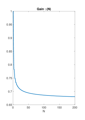
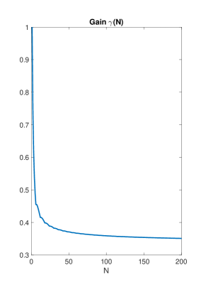
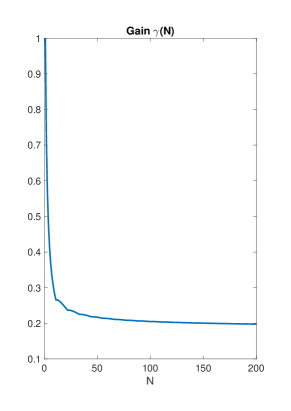
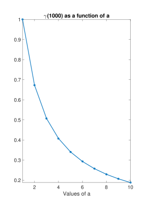
Figure 2: Top left: $a=2$, Top right: $a=5$, Bottom left: $a=10$, Bottom right: evolution of $\gamma(1000)$ as a function of $a$

2.2.2 Introducing dependence

The following discussion on possible extensions can be omitted on a first reading. There are numerous possible variations around the basic algorithm presented above. A practically important extension related to the order in which variables are drawn is discussed in Section 4 in the general context of latent variable models. There is another possible extension worth mentioning here. Close inspection of the proof of $\pi-$reversibility of $\mathring{P}^{N}$ in Theorem 1 suggests that conditional independence of $u^{(1)},\ldots,u^{(N)}$ is not a requirement. Define $\mathfrak{u}^{(-k)}:=\left(u^{(1)},\ldots,u^{(k-1)},u^{(k+1)},\ldots,u^{(N)}\right)$.

Theorem 2.

Let $N\geq 1$ and for any $x,y\in\mathsf{X}$ let $Q_{x,y}^{N}({\rm d}\mathfrak{u})$ be a probability distribution on $\big{(}\mathfrak{U},\mathcal{U}^{\otimes N}\big{)}$ such that all its marginals are identical and equal to $Q_{x,y}(\cdot)$. Assume that

$$Q_{1}^{N}\big{(}x,{\rm d}(y,\mathfrak{u},k)\big{)} :=q(x,{\rm d}y)Q_{x,y}^{N}({\rm d}\mathfrak{u})\frac{\mathring{r}_{u^{(k)}}(x,y)}{\sum_{i=1}^{N}\mathring{r}_{u^{(i)}}(x,y)},$$

$$Q_{2}^{N}\big{(}x,{\rm d}(y,\mathfrak{u},k)\big{)} :=q(x,{\rm d}y)\frac{1}{N}\bar{Q}_{x,y}({\rm d}u^{(k)})Q_{y,x}^{N}({\rm d}\mathfrak{u}^{(-k)}\mid u^{(k)}).$$

Then $\mathring{P}^{N}$ with acceptance ratio $\mathring{r}_{\mathfrak{u}}^{N}(x,y)$ as in (12) is $\pi-$reversible. Further, if $u^{(1)},\ldots,u^{(N)}$ are exchangeable with respect to $Q_{x,y}^{N}({\rm d}\mathfrak{u})$ then all the comparison results in Theorem 1 still hold.

Proof.

One can check that

$$\frac{\pi({\rm d}y)Q_{2}^{N}\big{(}y,{\rm d}(x,\mathfrak{u},k)\big{)}}{\pi({\rm d}x)Q_{1}^{N}\big{(}x,{\rm d}(y,\mathfrak{u},k)\big{)}} =\frac{\pi({\rm d}y)q(y,{\rm d}x)\frac{1}{N}\bar{Q}_{y,x}({\rm d}u^{(k)})Q_{x,y}^{N}({\rm d}\mathfrak{u}^{(-k)}\mid u^{(k)})}{\pi({\rm d}x)q(x,{\rm d}y)Q_{x,y}({\rm d}u^{(k)})Q_{x,y}^{N}({\rm d}\mathfrak{u}^{(-k)}\mid u^{(k)})\frac{\mathring{r}_{u^{(k)}}(x,y)}{\sum_{i=1}^{N}\mathring{r}_{u^{(i)}}(x,y)}}$$

$$=\mathring{r}_{u^{(k)}}(x,y)\frac{1/N}{\frac{\mathring{r}_{u^{(k)}}(x,y)}{N\times\mathring{r}_{\mathfrak{u}}^{N}(x,y)}}=\mathring{r}_{\mathfrak{u}}^{N}(x,y),$$

which remains the same as in (12). The exchangeability assumption ensures that (15) holds. ∎

Example 6.

The following is a short discussion of a scenario which may be relevant in practice. Assume that it is possible to sample $u^{\left(1\right)}$ from $Q_{x,y}(\cdot)$ but that this is computationally expensive, as is the case for sampling exactly from Markov random fields such as the Ising model. One could suggest sampling the remaining samples $\mathfrak{u}^{(-1)}$ as defined in $Q_{1}^{N}(\cdot,\cdot)$ using a $Q_{x,y}-$reversible Markov transition probability $K_{x,y}$ (and similarly for $Q_{y,x}(\cdot)$ in $Q_{2}^{N}(\cdot,\cdot)$ using $K_{y,x}$), which will in general be far less expensive. Here $Q_{1}^{N}(\cdot,\cdot)$ corresponds to sampling

$$u^{(1:N)}\sim Q_{x,y}({\rm d}u^{(1)})K_{x,y}(u^{(1)},{\rm d}u^{(2)})\ldots K_{x,y}(u^{(N-1)},{\rm d}u^{(N)}).$$

In order to describe sampling in $Q_{2}^{N}(\cdot,\cdot)$, we first establish a convenient expression for $Q_{x,y}^{N}({\rm d}\mathfrak{u}^{(-k)}\mid u^{(k)})$ for $x,y\in\mathsf{X}^{2}$ and $k=1,\ldots,N$. By reversibility of $K_{x,y}$, we have for $k=1,\ldots,N$ (with straightforward conventions for $k\in[N]$)

$$Q_{x,y}({\rm d}u^{(1)})\prod_{i=2}^{N}K_{x,y}(u^{(i-1)},{\rm d}u^{(i)})=Q_{x,y}({\rm d}u^{(k)})\prod_{i=2}^{k}K_{x,y}(u^{(i)},{\rm d}u^{(i-1)})\prod_{i=k+1}^{N}K_{x,y}(u^{(i-1)},{\rm d}u^{(i)})$$

from which one obtains the desired conditional, and deduces that sampling the auxiliary variables in $Q_{2}^{N}(\cdot,\cdot)$ consists of sampling $k\sim\mathcal{U}\{1,2,\ldots,N\}$, $u^{(k)}\sim\bar{Q}_{x,y}(\cdot)$, and then simulate the rest of the chain “forward” and “backward” as follows

$$(u^{(k-1)},\ldots,u^{(1)})\sim\prod_{i=2}^{k}K_{y,x}(u^{(i)},{\rm d}u^{(i-1)}),\quad(u^{(k+1)},\ldots,u^{(N)})\sim\prod_{i=k+1}^{N}K_{y,x}(u^{(i-1)},{\rm d}u^{(i)}).$$

Note that in this case, Remark 2 does not hold. While sampling $k$ is still not necessary in $Q_{1}^{N}(\cdot,\cdot)$, sampling $k$ in $Q_{2}^{N}(\cdot,\cdot)$ is required. The last part of the theorem is applicable by averaging over the set of permutations of $[N]$

$$Q_{x,y}^{N}\big{(}{\rm d}\mathfrak{u}\big{)}=\frac{1}{N!}\sum_{\sigma\in\mathfrak{S}}Q_{x,y}({\rm d}u^{(\sigma(1))})K_{x,y}(u^{(\sigma(1))},{\rm d}u^{(\sigma(2))})\ldots K_{x,y}(u^{(\sigma(N-1))},{\rm d}u^{(\sigma(N))}),$$

and noting that for $k\in[N]$ and by using the reversibility as above for each $\sigma\in\mathfrak{S}$ leads to

$$Q_{x,y}^{N}\big{(}{\rm d}\mathfrak{u}\big{)}=Q_{x,y}({\rm d}u^{(k)})\frac{1}{N!}\sum_{\sigma\in\mathfrak{S}}\prod_{i=2}^{\sigma^{-1}(k)}K_{x,y}(u^{(\sigma(i))},{\rm d}u^{(\sigma(i-1))})\prod_{i=\sigma^{-1}(k)+1}^{N}K_{x,y}(u^{(\sigma(i-1))},{\rm d}u^{(\sigma(i))}).$$

We do not investigate this algorithm further here.

3 Improving PMR algorithms with AIS

Before moving on to more complex scenarios in Section 4, we focus in this section on the averaging of acceptance ratios in the specific context of our running Example 4. The exchange algorithm (Murray et al., 2006), described in Example 3, exploits the fact that for $\theta,\theta^{\prime}\in\Theta$ and $u\sim\ell_{\theta^{\prime}}(\cdot)$, the ratio $g_{\theta}\big{(}u\big{)}/g_{\theta^{\prime}}\big{(}u\big{)}$ is an estimator of $C_{\theta}/C_{\theta^{\prime}}$. Another possible estimator of $C_{\theta}/C_{\theta^{\prime}}$, based on AIS (Crooks, 1998; Neal, 2001), was also used in Murray et al. (2006). It has the advantage that it involves a tuning parameter which can be used to reduce the variability of the estimator, and hence improve the theoretical performance of exchange type algorithms. It has recently been established theoretically that this approach can beat the curse of dimensionality by reducing complexity from exponential to polynomial in the problem dimension Andrieu et al. (2016); Beskos et al. (2014). This is however at the expense of an additional computational cost. In this section, we show that the AIS based exchange algorithm can be reinterpreted as a PMR algorithm of the form (9). It is thus straightforward to extend this methodology through Algorithm 1 so as to use acceptance ratio estimators obtained through averaging.

3.1 AIS based exchange algorithm and its average acceptance ratio form

The estimator $g_{\theta}\big{(}u\big{)}/g_{\theta^{\prime}}\big{(}u\big{)}$ for $u\sim\ell_{\theta^{\prime}}(\cdot)$ of the ratio of $C_{\theta}/C_{\theta^{\prime}}$ may be very variable when the functions $g_{\theta}(\cdot)$ and $g_{\theta^{\prime}}(\cdot)$ differ too much. The basic idea behind AIS consists of rewriting the ratio of interest as a telescoping product of ratios of normalising constants corresponding to a sequence of artificial probability densities

$$\mathscr{P}_{\theta,\theta^{\prime},T}:=\big{\{}\pi_{\theta,\theta^{\prime},t}(\cdot),t=0,\ldots,T+1\big{\}}$$

for some $T\geq 1$ evolving from $\pi_{\theta,\theta^{\prime},0}(u)=\ell_{\theta^{\prime}}(u)$ to $\pi_{\theta,\theta^{\prime},T+1}(u)=\ell_{\theta}(u)$; i.e. $\pi_{\theta,\theta^{\prime},t}(u)=f_{\theta,\theta^{\prime},t}(u)/C_{\theta,\theta^{\prime},t}$ where $f_{\theta,\theta^{\prime},t}(u)$ can be computed pointwise but $C_{\theta,\theta^{\prime},t}$ is intractable. More precisely one rewrites $C_{\theta}/C_{\theta^{\prime}}=\prod_{t=0}^{T}C_{\theta,\theta^{\prime},t+1}/C_{\theta,\theta^{\prime},t}$ (with $C_{\theta,\theta^{\prime},0}=C_{\theta^{\prime}}$ and $C_{\theta,\theta^{\prime},T+1}=C_{\theta}$) where the densities $\big{\{}f_{\theta,\theta^{\prime},t}(\cdot),t=1,\ldots,T\big{\}}$ are such that estimating each term $C_{\theta,\theta^{\prime},t+1}/C_{\theta,\theta^{\prime},t}$ can be performed efficiently using the technique above for example. Good performance therefore necessitates that successive unnormalised densities are close (and become ever closer as $T$ increases). A naive implementation would require exact sampling from each of the intermediate probability distributions but the remarkable fact noticed independently in Crooks (1998) and Neal (2001) is that the estimators involved in the product may arise from an inhomogeneous Markov chain, therefore rendering the algorithm highly practical. The following proposition establishes that this algorithm is of the same form as $\mathring{P}$ given in (9).

Proposition 1.

Assume the set-up of Example 1 and for all $\theta,\theta^{\prime}\in\Theta$, let

1. $\mathscr{F}_{\theta,\theta^{\prime},T}=\big{\{}f_{\theta,\theta^{\prime},t}(\cdot),t=0,\ldots,T+1\big{\}}$ be a family of tractable unnormalised densities of $\mathscr{P}_{\theta,\theta^{\prime},T}$ such that for $t=0,\ldots,T$

   1. $f_{\theta,\theta^{\prime},t}(\cdot)$ and $f_{\theta,\theta^{\prime},t+1}(\cdot)$ have the same support,

   2. for any $u\in\mathsf{Y}$

      $$f_{\theta,\theta^{\prime},0}(u)=g_{\theta^{\prime}}(u),\quad f_{\theta,\theta^{\prime},T+1}(u)=g_{\theta}(u),\quad f_{\theta,\theta^{\prime},t}(u)=f_{\theta^{\prime},\theta,T+1-t}(u),$$

2. $\mathscr{R}_{\theta,\theta^{\prime},T}=\big{\{}R_{\theta,\theta^{\prime},t}(\cdot,\cdot)\colon\mathsf{Y}\times\mathcal{Y}\to[0,1],t=1,\ldots,T\big{\}}$ be a family of Markov transition kernels such that for any $t=1,\ldots,T$

   1. $R_{\theta,\theta^{\prime},t}(\cdot,\cdot)$ is $\pi_{\theta,\theta^{\prime},t}-$reversible,

   2. $R_{\theta,\theta^{\prime},t}(\cdot,\cdot)=R_{\theta^{\prime},\theta,T+1-t}(\cdot,\cdot)$,

3. $Q_{\theta,\theta^{\prime}}(\cdot)$ be the probability distributions $\big{(}\mathsf{U},\mathcal{U}\big{)}$, where $\mathsf{U}:=\mathcal{\mathsf{Y}}^{T+1}$, defined for $u:=(u_{0},\ldots,u_{T})\in\mathsf{U}$ as

   $$\;Q_{\theta,\theta^{\prime}}({\rm d}u):= \ell_{\theta^{\prime}}({\rm d}u_{0})\prod_{t=1}^{T}R_{\theta,\theta^{\prime},t}(u_{t-1},{\rm d}u_{t}),$$ (16)

   and $\varphi$ the involution reversing the order of the components of $u$; i.e. $\varphi(u_{0},u_{1},\ldots,u_{T}):=(u_{T},u_{T-1},\ldots,u_{0})$ for all $u\in\mathsf{U}$.

Then for any $\theta,\theta^{\prime}\in\Theta$ and any $u\in\mathsf{U}$

$$\bar{Q}_{\theta,\theta^{\prime}}({\rm d}u)=\ell_{\theta^{\prime}}({\rm d}u_{T})\prod_{t=1}^{T}R_{\theta^{\prime},\theta,T-t+1}(u_{T-t+1},{\rm d}u_{T-t}),$$

and

$$\frac{\bar{Q}_{\theta^{\prime},\theta}({\rm d}u)}{Q_{\theta,\theta^{\prime}}({\rm d}u)}=\frac{C_{\theta^{\prime}}}{C_{\theta}}\prod_{t=0}^{T}\frac{f_{\theta,\theta^{\prime},t+1}(u_{t})}{f_{\theta,\theta^{\prime},t}(u_{t})}.$$

The AIS based exchange algorithm of Murray et al. (2006) corresponds to $\mathring{P}$ in (9) with proposal distribution

$$Q_{1}(\theta,{\rm d}(\theta^{\prime},u))=q(\theta,{\rm d}\theta^{\prime})Q_{\theta,\theta^{\prime}}({\rm d}u)$$

and its complementary kernel

$$Q_{2}(\theta,{\rm d}(\theta^{\prime},u))=q(\theta,{\rm d}\theta^{\prime})\bar{Q}_{\theta,\theta^{\prime}}({\rm d}u).$$

Its acceptance ratio on $\mathring{\mathsf{S}}$ is

$$\mathring{r}_{u}(\theta,\theta^{\prime})=\frac{q(\theta^{\prime},\theta)}{q(\theta,\theta^{\prime})}\frac{\eta(\theta^{\prime})}{\eta(\theta)}\frac{g_{\theta^{\prime}}(\mathfrak{y})}{g_{\theta}(\mathfrak{y})}\prod_{t=0}^{T}\frac{f_{\theta,\theta^{\prime},t+1}(u_{t})}{f_{\theta,\theta^{\prime},t}(u_{t})}.$$ (17)

Proof.

Since $Q_{\theta,\theta^{\prime}}(\varphi(A))=\bar{Q}_{\theta,\theta^{\prime}}(A)$, we can check that the pair $Q_{1}(x,\cdot)$, $Q_{2}(x,\cdot)$ satisfy the assumption of Theorem 5 in Appendix A. Moreover, by the symmetry assumption on $\mathscr{R}_{\theta,\theta^{\prime},T}$, we obtain

$$\bar{Q}_{\theta,\theta^{\prime}}({\rm d}u) =\ell_{\theta^{\prime}}({\rm d}u_{T})\prod_{t=1}^{T}R_{\theta,\theta^{\prime},t}(u_{T-t+1},{\rm d}u_{T-t})$$

$$=\ell_{\theta^{\prime}}({\rm d}u_{T})\prod_{t=1}^{T}R_{\theta^{\prime},\theta,T-t+1}(u_{T-t+1},{\rm d}u_{T-t}),$$

so we can apply Theorem 6 in Appendix B with $\mu_{0}=\ell_{\theta^{\prime}}$, $\mu_{\tau+1}=\ell_{\theta}$, $\tau=T$ and $\mu_{t}=\pi_{\theta,\theta^{\prime},t}$ and $\Pi_{t}=R_{\theta,\theta^{\prime},t}$ for $t=1,\ldots,T$ to show that $\bar{Q}_{\theta^{\prime},\theta}(\cdot)$ is absolutely continuous with respect to $Q_{\theta,\theta^{\prime}}(\cdot)$ and the expression for the corresponding Radon-Nikodym derivative ensures that (10) is indeed equal to (17). ∎

By selecting an appropriate sequence of intermediate distributions $\mathscr{P}_{\theta,\theta^{\prime},T}$ as detailed in Section 3.3, the variability of this noisy acceptance ratio can be reduced by increasing $T$. Another approach to reduce variability is given in Algorithm 2 which consists of averaging acceptance ratios as described in Algorithm 1. For $T=0$ and $N>1$ Algorithm 2 reduces to that in Example 4, for $N=1$ and $T>0$, we recover the exchange algorithm with bridging of Murray et al. (2006) and for $T=0$ and $N=1$, this reduces to the exchange algorithm. Our generalisation presents a clear computational interest: while sampling a realisation of the Markov chain defined by $Q_{\theta,\theta^{\prime}}(\cdot)$ is fundamentally a serial operation, sampling $N$ independent such realisations is trivially parallelisable. On an ideal parallel computer, running the algorithm for any $N>1$ or $N=1$ would take the same amount of the user’s time. We explore numerically combinations of the parameters $T$ and $N$ in Section 3.3.

1

2

Input: Current state $\theta_{n}=\theta$.

3

Output: Next sample $\theta_{n+1}$

4

5Sample $\theta^{\prime}\sim q(\theta,\cdot)$ and $v\sim\mathcal{U}(0,1)$.

6 if $v\leq 1/2$ then

7      

8      for $i=1,\ldots,N$ do

9            

10            Sample $u_{0}^{(i)}\sim\ell_{\theta^{\prime}}(\cdot)$ and $u_{t}^{(i)}\sim R_{\theta,\theta^{\prime},t}(u_{t-1}^{(i)},\cdot)$, $t=1,\ldots,T$.

11      

12      Set $\theta_{n+1}=\theta^{\prime}$ with probability $\min\{1,\mathring{r}_{\mathfrak{u}}^{N}(\theta,\theta^{\prime})\}$ (see (17)), otherwise set $\theta_{n+1}=\theta$.

13else

14      

15      Sample $u_{T}^{(1)}\sim\ell_{\theta^{\prime}}(\cdot)$ and $u_{t-1}^{(1)}\sim R_{\theta,\theta^{\prime},t}(u_{t}^{(1)},\cdot)$, $t=T,\ldots,1$,

16       for $i=2,\ldots,N$, do

17            

18            Sample $u_{0}^{(i)}\sim\ell_{\theta}(\cdot)$ and $u_{t}^{(i)}\sim R_{\theta^{\prime},\theta,t}(u_{t-1}^{(i)},\cdot)$, $t=1,\ldots,T$.

19      

20      Set $\theta_{n+1}=\theta^{\prime}$ with probability $\min\{1,1/\mathring{r}_{\mathfrak{u}}^{N}(\theta^{\prime},\theta)\}$, otherwise set $\theta_{n+1}=\theta$.

Algorithm 2 MHAR for averaged AIS PMR estimators

3.2 Using a single sample from $\ell_{\theta^{\prime}}(\cdot)$ per iteration

This section can be omitted on a first reading. In Algorithm 2, each of the $N$ chains has a different initial point, which is a sample from an intractable distribution. Obtaining such a sample can be computationally expensive. Algorithm 3 is an alternative that only requires one such sample at each iteration. The proof that the associated Markov kernel is $\pi$-reversible can be derived from Theorem 2 in Section 2.2.2, hence we omit it.

Although computationally more expensive on a serial machine, we expect Algorithm 2 to have better statistical properties than Algorithm 3 as it uses independent chains to estimate the acceptance ratio. This is demonstrated experimentally in Section 3.3. Moreover, the computational advantage of Algorithm 3 is questionable on a parallel architecture, where one can in principle run all the chains in $Q_{1}^{N}(\cdot,\cdot)$ and $Q_{2}^{N}(\cdot,\cdot)$ of Algorithm 2 at the same time. In fact, Algorithm 2 may be even faster since all the chains in the backward move can be produced in parallel whereas this can not be done in Algorithm 3.

1

2

Input: Current sample $\theta_{n}=\theta$.

3

Output: New sample $\theta_{n+1}$

4

5Sample $\theta^{\prime}\sim q(\theta,\cdot)$ and $v\sim\mathcal{U}(0,1)$.

6 if $v\leq 1/2$ then

7      

8      Sample $u_{0}\sim\ell_{\theta^{\prime}}(\cdot)$.

9       for $i=1,\ldots,N$ do

10            

11            Set $u_{0}^{(i)}=u_{0}$ and sample $u_{t}^{(i)}\sim R_{\theta,\theta^{\prime},t}(u_{t-1}^{(i)},\cdot)$, $t=1,\ldots,T$.

12      

13      Set $\theta_{n+1}=\theta^{\prime}$ with probability $\min\{1,\mathring{r}_{\mathfrak{u}}^{N}(\theta,\theta^{\prime})\}$, otherwise set $\theta_{n+1}=\theta$.

14else

15      

16      Sample $u_{T}^{(1)}\sim\ell_{\theta^{\prime}}(\cdot)$ and $u_{t-1}^{(1)}\sim R_{\theta^{\prime},\theta,t}(u_{t}^{(1)},\cdot)$, $t=T,\ldots,1$,

17       for $i=2,\ldots,N$, do

18            

19            Set $u_{0}^{(i)}=u_{0}^{(1)}$ and sample $u_{t}^{(i)}\sim R_{\theta^{\prime},\theta,t}(u_{t-1}^{(i)},\cdot)$, $t=1,\ldots,T$.

20      

21      Set $\theta_{n+1}=\theta^{\prime}$ with probability $\min\{1,1/\mathring{r}_{\mathfrak{u}}^{N}(\theta^{\prime},\theta)\}$, otherwise set $\theta_{n+1}=\theta$.

Algorithm 3 MHAR for averaged AIS PMR estimators reduced computation

3.3 Numerical example: the Ising model

We illustrate the performance of Algorithms 2 and 3 on the Ising model used in statistical mechanics to model ferromagnetism. For $m,n\in\mathbb{N}$ we consider an $m\times n$ lattice $\Lambda$. Associated to each site $k\in\Lambda$ is a binary variable $\mathfrak{z}[k]\in\{-1,1\}$ representing the spin configuration of the site. The probability of a given configuration $u=\{\mathfrak{z}[k],k\in\Lambda\}$ depends on an energy function, or Hamiltonian, which may depend on some parameter $\theta$. A standard choice used in the absence of an external magnetic field is

$$H_{\theta}(\mathfrak{z})=-\theta\sum_{i\sim j}\mathfrak{z}[i]\mathfrak{z}[j],$$

where $i\sim j$ denotes a pair or adjacent sites and $\theta\in\Theta=\mathbb{R}_{+}$ is referred to as the inverse temperature parameter. The probability of configuration $\mathfrak{z}$ for temperature $\theta^{-1}$ is given by $\ell_{\theta}(\mathfrak{z})=g_{\theta}(\mathfrak{z})/C_{\theta}$ where $g_{\theta}(\mathfrak{z})=\exp(-H_{\theta}(\mathfrak{z}))$ and $C_{\theta}=\sum_{\mathfrak{z}\in\{0,1\}^{|\Lambda|}}g_{\theta}(\mathfrak{z})$ is the intractable and $\theta$-dependent normalising constant. In the following experiment, we perform Bayesian estimation of $\theta$ given a $20\times 30$ configuration $\mathfrak{y}$ drawn from $\ell_{\theta^{*}}(\cdot)$ for $\theta^{\ast}=0.35$, which is slightly above the critical (inverse) temperature $\log(1+\sqrt{2})/2$, resulting in strongly correlated neighbouring sites. The prior distribution for $\theta$ is taken to be the uniform distribution on $(0,10)$. The difficulty here is that computing $C_{\theta}$ requires the summation of $2^{600}$ terms, which is computationally infeasible.

The sequence of intermediate distributions used within AIS relies on a geometric annealing schedule for the unnormalised densities of the annealing distributions that is

$$f_{\theta,\theta^{\prime},t}(\mathfrak{z})=g_{\theta}(\mathfrak{z})^{1-\beta_{t}}g_{\theta^{\prime}}(\mathfrak{z})^{\beta_{t}}=g_{\theta(1-\beta_{t})+\theta^{\prime}\beta_{t}}(\mathfrak{z}),\quad\beta_{t}=1-\frac{t}{T+1},\quad t=0,1,\ldots,T+1.$$

Sampling from the intractable distribution is performed approximately by running Wolff’s algorithm, essentially an MCMC kernel iterated for $100$ iterations. For $\theta,\theta^{\prime}\in\Theta$ and $t=1,\ldots,T$ we chose $R_{\theta,\theta^{\prime},t}$ to be a single iteration of the MCMC kernel of the Wolff’s algorithm targeting $\ell_{\theta(1-\beta_{t})+\theta^{\prime}\beta_{t}}(\cdot)$. We ran both Algorithms 2 and 3 for all of the combinations of $N=1,10,20,\ldots,100$ and $T=1,2,\ldots,10,20,\ldots,100$. For each run, $K=10^{6}$ samples were generated and the last $3K/4$ of them were used to compute the IAC of the sequence $\{\theta_{i},i=1\geq 1\}$. Figure 3 concentrates on the two extreme scenarios where $N=1$ and when $T=0$, that correspond to the exchange algorithm with bridging as in Murray et al. (2006) and our novel averaging algorithm applied to Example 4, respectively. The figure suggests that our algorithm is computationally superior on an ideal parallel machine, at least for the present example.

The rest of the results are shown in Figure 4. The results are organised in order to contrast Algorithms 2 and 3. The figure suggests that Algorithm 2, which uses multiple samples from the intractable distribution per iteration, is uniformly better, as expected. Finally, although for large $T$ the performances of the two algorithms get closer, for small $T$ the advantage of using more samples from the intractable distribution, i.e. using Algorithm 2 is more significant.

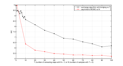
Figure 3: IAC for $\theta$ in the Ising model vs (a) the number of averaged ratios $N=1,10,20,\ldots,100$ for $T=0$ (red/grey) and (b) the number of annealing steps $T=0,1,2,\ldots,10,20,\ldots,100$ for $N=1$ (black).

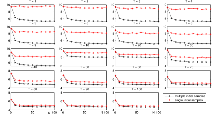
Figure 4: IAC for $\theta$ for the combinations of $N=1,10,20,\ldots,100$ and $T=1,2,\ldots,10,20,\ldots,100$. Each plot shows IAC vs $N$ for a fixed $T$.

4 PMR algorithms for latent variable models

4.1 Latent variable models

We consider here sampling from a distribution that is the marginal of a given joint distribution. More precisely, let $(\Theta,\mathcal{E})$ and $(\mathsf{Z},\mathcal{Z})$ be two measurable spaces, and define the product spaces $\mathsf{X}=\Theta\times\mathsf{Z}$ and $\mathcal{X}=\mathcal{E}\otimes\mathcal{Z}$ the corresponding product $\sigma$-algebra. Let $\pi({\rm d}x):=\pi({\rm d}(\theta,z))$ be a probability distribution on $(\mathsf{X},\mathcal{X})$ which is assumed known up to a normalising constant. Our primary interest is to sample from the marginal distribution of $\theta$,

$$\pi({\rm d}\theta)=\int_{\mathsf{Z}}\pi\big{(}{\rm d}(\theta,z)\big{)},$$

assumed to be intractable, i.e. no useful density is available, even up to a normalising constant. The doubly intractable scenario covered so far falls into this category. It exploits the fact that

$$\pi\big{(}\theta,z\big{)}\propto\eta(\theta)g_{\theta}(\mathfrak{y})\frac{h_{\mathfrak{y}}(z)}{g_{\theta}(z)}\ell_{\theta}\big{(}z\big{)},$$

has $\pi\big{(}\theta\big{)}\propto\eta(\theta)\ell_{\theta}\big{(}\mathfrak{y}\big{)}$ as marginals, but also the additional property that sampling from the intractable distribution $\ell_{\theta}\big{(}z\big{)}$ is possible. This latter property is fundamental to by-pass the intractability of the normalising constant, but also allows one to refresh $z$ at each iteration of the MCMC algorithm, in contrast with the pseudo-marginal approach. As a result the exchange algorithm defines an algorithm which directly targets $\pi(\theta)$ with a Markov chain defined on $(\Theta,\mathcal{E})$. This however turns out to be too specific and restrictive for numerous applications, such as state-space models.

Example 7.

We consider the well-known non-linear state-space, often used to assess the performance of inference methods for non-linear state-space models,

$$Z_{t} =Z_{t-1}/2+25Z_{t-1}/(1+Z_{t-1}^{2})+8\cos(1.2t)+V_{t},\quad t\geq 2$$

$$Y_{t} =Z_{t}^{2}/20+W_{t},\quad t\geq 1,$$

where $Z_{1}\sim\mathcal{N}(0,10)$, $V_{t}\overset{\mathrm{iid}}{\sim}\mathcal{N}(0,\sigma_{v}^{2})$, $W_{t}\overset{\mathrm{iid}}{\sim}\mathcal{N}(0,\sigma_{w}^{2})$. The parameter of primary interest is $\theta=(\sigma_{v}^{2},\sigma_{w}^{2})$ and is ascribed the prior $(\sigma_{v}^{2},\sigma_{w}^{2})\overset{\mathrm{iid}}{\sim}\mathcal{IG}(0.01,0.01)$ where $\mathcal{IG}(a,b)$ is the inverse gamma distribution with shape and scale parameters $a$ and $b$. The aim is to infer $x=(\theta,z)$, where the latent variable is $z=z_{1:P}$ for some $P>1$, from a particular data set $Y_{1:P}=y_{1:P}$.

Ideally we would like to use the following “marginal” algorithm. Let $q(\theta,\cdot)$ be a Markov kernel on $(\Theta,\mathcal{E})$ such that for each $\theta\in\Theta$, $q(\theta,\cdot)$ admits a density $q(\theta,\cdot)$ with respect to ${\rm d}\theta^{\prime}$. The acceptance rate of the MH algorithm with proposal kernel $q(\cdot,\cdot)$ targeting $\pi(\theta)$ is

$$r(\theta,\theta^{\prime})=\frac{q(\theta^{\prime},\theta)\pi(\theta^{\prime})}{q(\theta,\theta^{\prime})\pi(\theta)}.$$ (18)

The latter cannot be evaluated in numerous scenarios of interest and the aim of this section is to extend the framework developed for the doubly intractable scenario to the more general situation where sampling of the latent variable must be included in the MCMC scheme itself and cannot be performed exactly. This results in an algorithm tar-getting the distribution $\pi(\mathrm{d}(\theta,z))$. It turns out that the framework developed in Section 2 can also be easily adapted to this scenario. More precisely, here we have $x=(\theta,z)$ and $y=(\theta^{\prime},z^{\prime})$ and the only difference with the developments of Algorithm 1 is concerned with the order in which the variables are sampled. In Algorithm 1 we have assumed a specific sampling order for the variables involved, that is the auxiliary variable copies are sampled after the proposed value $y$. Here we are going to consider the scenario where $\theta^{\prime}$ is sampled first, then the auxiliary variables $u^{(1)},\ldots,u^{(N)}$ are sampled from a kernel $Q_{\theta,\theta^{\prime},z}({\rm d}u)$ and $z^{\prime}$ is proposed last, conditional upon the auxiliary variables $\theta,\theta^{\prime},z$ and $u^{(1)},\ldots,u^{(N)}$. The resulting expression for the acceptance ratio remains the same as that used in Algorithm 1 since it is not affected by the order in which the variables are sampled.

4.2 AIS within MH for latent variable models

Neal (2004) suggested to use AIS, as described in Section 2 and Theorem 6 in Appendix B, in order to achieve sampling from $\pi$. The idea should be clear upon noticing that for $\theta\in\Theta$ fixed, $\pi(\theta)$ is the normalising constant of the conditional distribution for $z$ that is proportional to $\pi(\theta,z)$, that is $\pi_{\theta}(z)\propto\pi(\theta,z)$. To estimate the ratio $\pi(\theta^{\prime})/\pi(\theta)$ one therefore defines a sequence of artificial probability densities

$$\mathscr{P}_{\theta,\theta^{\prime},T}:=\big{\{}\pi_{\theta,\theta^{\prime},t},t=0,\ldots,T+1\big{\}}$$

for some $T\geq 1$ evolving from $\pi_{\theta,\theta^{\prime},0}(z)=\pi_{\theta}(z)$ to $\pi_{\theta,\theta^{\prime},T+1}(z)=\pi_{\theta^{\prime}}(z)$, through a sequence of unnormalised intermediate probability densities $\mathscr{F}_{\theta,\theta^{\prime},T}=\{f_{\theta,\theta^{\prime},t},t=0,\ldots,T+1\}$. The following proposition establishes that this algorithm is conceptually of the same form as $\mathring{P}$ given in (9) and this allows us to extend this methodology through Algorithm 1.

Proposition 2.

Consider the latent variable model given in the introduction of Section 4 and for any $\theta,\theta^{\prime}\in\Theta$ let

1. $\mathscr{F}_{\theta,\theta^{\prime},T}=\big{\{}f_{\theta,\theta^{\prime},t},t=0,\ldots,T+1\big{\}}$ be a family of tractable unnormalised densities of $\mathscr{P}_{\theta,\theta^{\prime},T}$ defined on $\big{(}\mathsf{Z},\mathcal{Z}\big{)}$ such that

   1. for $t=0,\ldots,T$, $f_{\theta,\theta^{\prime},t}$ and $f_{\theta,\theta^{\prime},t+1}$ have the same support,

   2. for any $z\in\mathsf{Z}$ and $t=1,\ldots,T$ $f_{\theta,\theta^{\prime},t}(z)=f_{\theta^{\prime},\theta,T+1-t}(z)$,

   3. $f_{\theta,\theta^{\prime},0}(z)=\pi(\theta,z)$ and $f_{\theta,\theta^{\prime},T+1}(z)=\pi(\theta^{\prime},z)$,

2. $\mathscr{R}_{\theta,\theta^{\prime},T}=\big{\{}R_{\theta,\theta^{\prime},t}(\cdot,\cdot)\colon\mathsf{Z}\times\mathcal{Z}\to[0,1],t=1,\ldots,T\big{\}}$ be a family of Markov transition kernels such that for any $t=1,\ldots,T$

   1. $R_{\theta,\theta^{\prime},t}(\cdot,\cdot)$ is $\pi_{\theta,\theta^{\prime},t}-$reversible,

   2. $R_{\theta,\theta^{\prime},t}(\cdot,\cdot)=R_{\theta^{\prime},\theta,T-t+1}(\cdot,\cdot)$,

3. $R_{\theta}(\cdot,\cdot)\colon\mathsf{Z}\times\mathcal{Z}\to[0,1]$ be a $\pi_{\theta}-$reversible Markov transition kernel,

4. $Q_{\theta,\theta^{\prime},z}(\cdot)$ be probability distributions on $\big{(}\mathsf{U},\mathcal{U}\big{)}$ where $\mathsf{U}:=\mathcal{\mathsf{Z}}^{T+1}$ defined for

   $$Q_{\theta,\theta^{\prime},z}({\rm d}u) =R_{\theta}(z,{\rm d}u_{0})\prod_{t=1}^{T}R_{\theta,\theta^{\prime},t}(u_{t-1},{\rm d}u_{t}),$$ (19)

   and let $\varphi$ be the involution which reverses the order of the components of $u$; i.e. $\varphi(u_{0},u_{1},\ldots,u_{T}):=(u_{T},u_{T-1},\ldots,u_{0})$ for all $u\in\mathsf{U}$.

Then for any $(\theta,z),(\theta^{\prime},z^{\prime}),u\in\big{(}\Theta\times\mathsf{\mathsf{Z}}\big{)}^{2}\times\mathsf{U}$

$$\bar{Q}_{\theta,\theta^{\prime},z}({\rm d}u)=R_{\theta}(z,{\rm d}u_{T})\prod_{t=1}^{T}R_{\theta^{\prime},\theta,t}(u_{t},{\rm d}u_{t-\text{1}}),$$ (20)

and

$$\frac{\pi_{\theta^{\prime}}({\rm d}z^{\prime})\bar{Q}_{\theta^{\prime},\theta,z^{\prime}}({\rm d}u)R_{\theta}(u_{0},{\rm d}z)}{\pi_{\theta}({\rm d}z)Q_{\theta,\theta^{\prime},z}({\rm d}u)R_{\theta^{\prime}}(u_{T},{\rm d}z^{\prime})}=\frac{\pi(\theta)}{\pi(\theta^{\prime})}\prod_{t=0}^{T}\frac{f_{\theta,\theta^{\prime},t+1}(u_{t})}{f_{\theta,\theta^{\prime},t}(u_{t})}.$$ (21)

The AIS MCMC algorithm of Neal (2004) for latent variable models corresponds to $\mathring{P}$ in Theorem 5 with $x=(\theta,z)$ and $y=(\theta^{\prime},z^{\prime})$, the proposal kernel

$$Q_{1}(x,{\rm d}(y,u)):=q(\theta,{\rm d}\theta^{\prime})Q_{\theta,\theta^{\prime},z}({\rm d}u)R_{\theta^{\prime}}(u_{T},{\rm d}z^{\prime})$$

and its complementary kernel

$$Q_{2}(x,{\rm d}(y,u)):=q(\theta,{\rm d}\theta^{\prime})\bar{Q}_{\theta,\theta^{\prime},z}({\rm d}u)R_{\theta^{\prime}}(u_{0},{\rm d}z^{\prime}).$$

Its acceptance ratio on $\mathring{\mathsf{S}}$ is

$$\mathring{r}_{u}(\theta,z;\theta^{\prime},z^{\prime})=\frac{\pi({\rm d}x^{\prime})Q_{2}(y,{\rm d}(x,u))}{\pi({\rm d}x)Q_{1}(x,{\rm d}(y,u))}=\frac{q(\theta^{\prime},\theta)}{q(\theta,\theta^{\prime})}\prod_{t=0}^{T}\frac{f_{\theta,\theta^{\prime},t+1}(u_{t})}{f_{\theta,\theta^{\prime},t}(u_{t})}.$$

Proof.

Since $\bar{Q}_{\theta,\theta^{\prime},z}(A)=Q_{\theta,\theta^{\prime},z}(\varphi(A))$, we can check that the pair $Q_{1}(x,\cdot)$, $Q_{2}(x,\cdot)$ satisfy the assumption of Theorem 5 in Appendix A. Next, using the symmetry assumption on $\mathscr{R}_{\theta,\theta^{\prime},T}$, we obtain

$$\bar{Q}_{\theta,\theta^{\prime},z}({\rm d}u) =R_{\theta}(z,{\rm d}u_{T})\prod_{t=1}^{T}R_{\theta^{\prime},\theta,T-t+1}(u_{T-t+1},{\rm d}u_{T-t})$$

and we can thus apply Theorem 6 in Appendix B (with $\tau=T+2$ intermediate distributions, two repeats $\mu_{0}=\mu_{1}$ and $\mu_{\tau}=$ $\mu_{\tau+1}$, $\mu_{t}=\pi_{\theta,\theta^{\prime},t-1}$ for $t=2,\ldots,\tau-1$ and kernels $\Pi_{1}=R_{\theta}$, $\Pi_{\tau}=R_{\theta^{\prime}}$ and $\Pi_{t}=R_{\theta,\theta^{\prime},t-1}$ for $t=2,\ldots,\tau-1$) to show that $\pi_{\theta^{\prime}}\times\bar{Q}_{\theta^{\prime},\theta,\cdot}\times R_{\theta}$ is absolutely continuous with respect to $\pi_{\theta}\times Q_{\theta,\theta^{\prime},\cdot}\times R_{\theta^{\prime}}$ and that the expression for the corresponding Radon-Nikodym derivative ensures that the acceptance ratio defined in (10) is indeed equal to (17). ∎

The standard choice made in Neal (2004) corresponds to $R_{\theta}(z,{\rm d}u_{0})=\delta_{z}\big{(}{\rm d}u_{0}\big{)}$, but more general choices are possible. As we shall see in the next section, a choice different from $\delta_{z}\big{(}{\rm d}u_{0}\big{)}$ can improve performance significantly when averaging acceptance ratios.

The variance of this unbiased estimator $\mathring{r}_{u}(\theta,z;\theta^{\prime},z^{\prime})$ of $r\big{(}\theta,\theta^{\prime}\big{)}$ can usually be tuned by increasing $T$, under natural smoothness conditions on the sequences $\mathscr{F}_{\theta,\theta^{\prime},T}$ for $T\geq 1$. An important point here is that although the approximated acceptance ratio is reminiscent of that of a MH algorithm targeting $\pi({\rm d}\theta)$, the present algorithm targets the joint distribution $\pi\big{(}{\rm d}(\theta,z)\big{)}$: the simplification occurs only because the random variable corresponding to $u_{T}$ in (19) will be approximately distributed according to $\pi_{\theta^{\prime}}(\cdot)$ when $T$ is large enough, under proper mixing conditions.

We note that the expression for $\mathring{r}_{u}(\theta,z;\theta^{\prime},z^{\prime})$ does not depend on either $z$ or $z^{\prime}$, and can in particular be calculated before sampling $z^{\prime}$. This is of importance in what follows and justifies the use of the simplified piece of notation $\mathring{r}_{u}(\theta,\theta^{\prime})$ below.

4.3 Averaging AIS based pseudo-marginal ratios

We show here how the algorithm of the previous section (Proposition 2) can be modified in order to average multiple ($N>1$) estimators $\mathring{r}_{u}(\theta,\theta^{\prime})$ of $r(\theta,\theta^{\prime})$ while preserving reversibility of the algorithm of interest. Let $u=(u_{0},\ldots,u_{T})\in\mathsf{U}=\mathsf{Z}^{T+1}$ and $k\in\{1,\ldots,N\}$.

Proposition 3.

Assume that the conditions of Proposition 2 hold. For $N\geq 1$ define the proposal kernels $Q_{1}^{N}(\cdot,\cdot)$ and $Q_{2}^{N}(\cdot,\cdot)$ on $\big{(}\mathsf{X}\times\mathsf{\mathfrak{U}}\times[k],\mathcal{X}\otimes\mathscr{U}\otimes\mathscr{P}[k]\big{)}$

$$Q_{1}^{N}\big{(}x;{\rm d}(y,\mathfrak{u},k)\big{)} =q(\theta,{\rm d}\theta^{\prime})\prod_{i=1}^{N}Q_{\theta,\theta^{\prime},z}({\rm d}u^{(i)})\frac{\mathring{r}_{u^{(k)}}(\theta,\theta^{\prime})}{\sum_{i=1}^{N}\mathring{r}_{u^{(i)}}(\theta,\theta^{\prime})}R_{\theta^{\prime}}(u_{T}^{(k)},{\rm d}z^{\prime}),$$ (22)

$$Q_{2}^{N}\big{(}x;{\rm d}(y,\mathfrak{u},k)\big{)} =q(\theta,{\rm d}\theta^{\prime})\frac{1}{N}\bar{Q}_{\theta,\theta^{\prime},z}({\rm d}u^{(k)})R_{\theta^{\prime}}(u_{0}^{(k)},{\rm d}z^{\prime})\prod_{i=1,i\neq k}^{N}Q_{\theta^{\prime},\theta,z^{\prime}}({\rm d}u^{(i)}).$$ (23)

Then one can implement $\mathring{P}^{N}$ corresponding to $\mathring{P}$ defined in Proposition 2, with $Q_{1}^{N}(\cdot,\cdot)$ and $Q_{2}^{N}(\cdot,\cdot)$ above and

$$\mathring{r}_{\mathfrak{u}}^{N}(\theta,\theta^{\prime})=\frac{1}{N}\sum_{i=1}^{N}\mathring{r}_{u^{(i)}}(\theta,\theta^{\prime}).$$

Proof.

One can check directly that $\mathring{r}^{N}(\theta,\theta^{\prime})$ is of the expected form despite the sampling order change

$$\frac{\pi({\rm d}y)Q_{2}^{N}\big{(}y,{\rm d}(x,\mathfrak{u},k)\big{)}}{\pi({\rm d}x)Q_{1}^{N}\big{(}x,{\rm d}(y,\mathfrak{u},k)\big{)}} =\frac{\pi({\rm d}y)q(\theta^{\prime},{\rm d}\theta)\frac{1}{N}\bar{Q}_{\theta,\theta^{\prime},z^{\prime}}({\rm d}u^{(k)})R_{\theta}(u_{0}^{(k)},{\rm d}z)\prod_{i=1,i\neq k}^{N}Q_{\theta,\theta^{\prime},z}({\rm d}u^{(i)})}{\pi({\rm d}x)q(\theta,{\rm d}\theta^{\prime})\prod_{i=1}^{N}Q_{\theta,\theta^{\prime},z}({\rm d}u^{(i)})\frac{\mathring{r}_{u^{(k)}}(\theta,\theta^{\prime})}{\sum_{i=1}^{N}\mathring{r}_{u^{(i)}}(\theta,\theta^{\prime})}R_{\theta^{\prime}}(u_{T}^{(k)},{\rm d}z^{\prime})}$$

$$=\frac{q(\theta^{\prime},\theta)\pi(\theta^{\prime})}{q(\theta,\theta^{\prime})\pi(\theta)}\frac{\pi_{\theta^{\prime}}(\mathrm{d}z^{\prime})\bar{Q}_{\theta^{\prime},\theta,z^{\prime}}({\rm d}u^{(k)})R_{\theta}(u_{0}^{(k)},{\rm d}z)}{\pi_{\theta}(\mathrm{d}z)Q_{\theta,\theta^{\prime},z}({\rm d}u^{(k)})R_{\theta^{\prime}}(u_{T}^{(k)},{\rm d}z^{\prime})}\mathring{r}_{u^{(k)}}^{-1}(\theta,\theta^{\prime})\frac{1}{N}\sum_{i=1}^{N}\mathring{r}_{u^{(i)}}(\theta,\theta^{\prime}).$$

∎

The implementation of the resulting asymmetric MCMC algorithm is described in Algorithm 4. The interest of introducing a general form for $R_{\theta}$ should now be clear: the standard choice $R_{\theta}\big{(}z,\cdot\big{)}=\delta_{z}(\cdot)$ introduces dependence among $u^{(1)},u^{(2)},\ldots,u^{(N)}$ which can be alleviated by the introduction of a more general ergodic transition, which may consist of an iterated reversible Markov transition of invariant distribution $\pi_{\theta}$. We also notice that some computational savings are possible. For example when $Q_{1}^{N}(\cdot,\cdot)$ is the distribution we sample from, the acceptance ratio does not depend on $k$, whose sampling can therefore be postponed until after a decision to accept has been made. The complementary update for which we sample from $Q_{2}^{N}(\cdot,\cdot)$ effectively does not require sampling $k$ which is set to $1$ in our implementation in Algorithm 4.

1

2

Input: Current sample $X_{n}=x=(\theta,z)$

3

Output: New sample $X_{n+1}$

4

5Sample $\theta^{\prime}\sim q(\theta,\cdot)$ and $v\sim\mathcal{U}(0,1)$.

6 if $v\leq 1/2$ then

7      

8      for $i=1,\ldots,N$ do

9            

10            Sample $u_{0}^{(i)}\sim R_{\theta}(z,\cdot)$ and $u_{t}^{(i)}\sim R_{\theta,\theta^{\prime},t}(u_{t-1}^{(i)},\cdot)$ for $t=1,\ldots,T$.

11      

12      Sample $k\sim\mathcal{P}\big{(}\mathring{r}_{u^{(1)}}(\theta,\theta^{\prime}),\ldots,\mathring{r}_{u^{(N)}}(\theta,\theta^{\prime})\big{)}$ and $z^{\prime}\sim R_{\theta^{\prime}}(u_{T}^{(k)},\cdot)$.

13       Set $X_{n+1}=(\theta^{\prime},z^{\prime})$ with probability $\min\{1,\mathring{r}_{\mathfrak{u}}^{N}(\theta,\theta^{\prime})\},$ otherwise set $X_{n+1}=x$.

14else

15      

16      Sample $u_{T}^{(1)}\sim R_{\theta}\big{(}z,\cdot\big{)}$, $u_{t-1}^{(1)}\sim R_{\theta^{\prime},\theta,t}(u_{t},\cdot)$ for $t=T,\ldots,1$ and $z^{\prime}\sim R_{\theta^{\prime}}(u_{0}^{(1)},\cdot)$.

17       for  $i=2,\ldots,N$, do

18            

19            Sample $u_{0}^{(i)}\sim R_{\theta^{\prime}}(z^{\prime},\cdot)$ and $u_{t}^{(i)}\sim R_{\theta^{\prime},\theta,t}(u_{t-1}^{(i)},\cdot)$ for $t=1,\ldots,T$.

20      

21      Set $X_{n+1}=(\theta^{\prime},z^{\prime})$ with probability $\min\{1,1/\mathring{r}_{\mathfrak{u}}^{N}(\theta^{\prime},\theta)\}$, otherwise set $X_{n+1}=x$.

Algorithm 4 MHAR for averaged AIS PMR estimators for general latent variable models

Example 8 (Example 7, ctd.).

In order to illustrate the interest of our approach, we generated data from the model for $P=500$, $\sigma_{v}^{2}=10$ and $\sigma_{w}^{2}=0.1$. The set-up for Algorithm 4 was as follows. We let $T=1$ and for $\theta,\theta^{\prime}\in\Theta$ the unnormalised density of the intermediate distribution was chosen to be $f_{\theta,\theta^{\prime},1}(z)=\pi((\theta+\theta^{\prime})/2,z)$. The MCMC kernel $R_{\theta,\theta^{\prime},1}(\cdot,\cdot)$ was a conditional SMC (cSMC) Andrieu et al. (2010) tar getting the intermediate distribution, with $M=100$ particles and the model transitions as proposal distributions; for convenience the cSMC kernel is described in Section 5. We used a normal random walk proposal with diagonal covariance matrix as a parameter proposal, where the standard deviations for $\sigma_{v}$ and $\sigma_{w}$ were $0.15$ and $0.08$ respectively. Performance, measured in terms of convergence to equilibrium and asymptotic variance for $N=1$, $N=10$ and $N=100$, is presented in Figure 6 and 11. For each set-up, $200$0 independent Monte Carlo runs of length 1000 each were used to assess convergence to the posterior mean, posterior second moment and median, via ensemble averages over the runs. We observe in Figure 6 that this simple approach improves performance and reduces time to convergence by approximately 50%. In addition to faster convergence, of the order of $30\%$, in terms of IAC in Figure 6. The estimated IAC values were obtained after discarding the first 300 iterations and by averaging over 2000 Monte Carlo runs. We present further new developments for this application in Section 4.5.

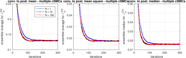
Figure 5: Convergence results for $\theta=(\sigma_{v}^{2},\sigma_{w}^{2})$ vs $N$ in Algorithm 4.

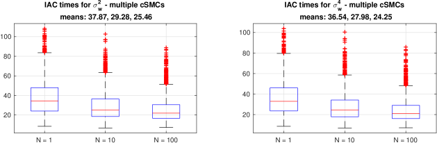
Figure 6: IAC for $\sigma_{w}^{2}$ and $\sigma_{w}^{4}$ vs $N$ in Algorithm 4.

4.4 Generalisations of MHAAR algorithms for latent variable models

We now discuss two generalisations of Algorithm 4 above which will prove crucial in Section 4.5, where we present our trans-dimensional example as an application of the methodology presented here, albeit in a scenario involving additional complications.

4.4.1 Annealing in a different space

The first generalisation is based on the main idea that condition 3 in Proposition 2 can be relaxed in the light of Theorem 6, and in particular allows the latent variable $z$ and auxiliary variables $u_{t}$ to live on different spaces.

Proposition 4.

Suppose that assumptions 1a-1b and 2 of Proposition 2 are satisfied with $\mathscr{F}_{\theta,\theta^{\prime},T},\mathscr{P}_{\theta,\theta^{\prime},T}$ and $\mathscr{R}_{\theta,\theta^{\prime},T}$ now defined on some space $\big{(}\mathsf{V},\mathcal{V}\big{)}$ (and $\mathsf{U:=\mathsf{V}}^{T+1}$), (therefore $\pi_{\theta,\theta^{\prime},0}\neq$$\pi_{\theta}$ , and $\pi_{\theta,\theta^{\prime},T+1}\neq\pi_{\theta^{\prime}}$ in general), and assumptions 1c and 3 replaced, for $\theta,\theta^{\prime}\in\Theta$ and $z,z^{\prime}\in\mathsf{Z}$, with

1. the endpoint conditions for the unnormalised densities are of the form

   $$f_{\theta,\theta^{\prime},0}(v) =\pi_{\theta,\theta^{\prime},0}(v)\pi(\theta),$$

   $$f_{\theta,\theta^{\prime},T+1}(v) =\pi_{\theta,\theta^{\prime},T+1}(v)\pi(\theta^{\prime}),$$

2. the existence of Markov transition kernels $\overrightarrow{R}_{\theta,\theta^{\prime},0}$,$\overleftarrow{R}_{\theta,\theta^{\prime},T+1}:\mathsf{Z}\times\mathcal{V}\rightarrow[0,1]$ and $\overrightarrow{R}{}_{\theta,\theta^{\prime},T+1}$,$\overleftarrow{R}_{\theta,\theta^{\prime},0}:\mathsf{V}\times\mathcal{Z}\rightarrow[0,1]$ such that

   $$\pi_{\theta}({\rm d}z)\overrightarrow{R}_{\theta,\theta^{\prime},0}(z,{\rm d}v) =\pi_{\theta,\theta^{\prime},0}({\rm d}v)\overleftarrow{R}_{\theta,\theta^{\prime},0}(v,{\rm d}z),$$

   $$\pi_{\theta,\theta^{\prime},T+1}({\rm d}v)\overrightarrow{R}_{\theta,\theta^{\prime},T+1}(v,{\rm d}z) =\pi_{\theta^{\prime}}({\rm d}z)\overleftarrow{R}{}_{\theta,\theta^{\prime},T+1}(z,{\rm d}v),$$

3. Define the proposal probability distributions on $\big{(}\mathsf{U},\mathcal{U}\big{)}$ such that for any $u\in\mathsf{U}=\mathsf{V}^{T+1}$,

   $$Q_{\theta,\theta^{\prime},z}\big{(}{\rm d}u\big{)} =\overrightarrow{R}_{\theta,\theta^{\prime},0}(z,{\rm d}u_{0})\prod_{t=1}^{T}R_{\theta,\theta^{\prime},t}(u_{t-1},{\rm d}u_{t}),$$

   and the involution $\varphi$ reversing the order of the components of $u$; i.e. $\varphi(u_{0},u_{1},\ldots,u_{T}):=(u_{T},u_{T-1},\ldots,u_{0})$ for all $u\in\mathsf{U}$.

Then for any $\big{(}(\theta,z),(\theta^{\prime},z^{\prime}),u\big{)}\in\big{(}\Theta\times\mathsf{\mathsf{Z}}\big{)}^{2}\times\mathsf{U}$

$$\bar{Q}_{\theta,\theta^{\prime},z}\big{(}{\rm d}u\big{)}=\overleftarrow{R}_{\theta^{\prime},\theta,T+1}(z,{\rm d}u_{T})\prod_{t=1}^{T}R_{\theta^{\prime},\theta,T-t+1}(u_{T-t+1},{\rm d}u_{T-t}),$$

and

$$\frac{\pi_{\theta^{\prime}}({\rm d}z^{\prime})\bar{Q}_{\theta^{\prime},\theta,z^{\prime}}({\rm d}u)\overleftarrow{R}_{\theta,\theta^{\prime},0}(u_{0},{\rm d}z)}{\pi_{\theta}({\rm d}z)Q_{\theta,\theta^{\prime},z}({\rm d}u)\overrightarrow{R}_{\theta,\theta^{\prime},T+1}(u_{T},{\rm d}z^{\prime})}=\frac{\pi(\theta)}{\pi(\theta^{\prime})}\prod_{t=0}^{T}\frac{f_{\theta,\theta^{\prime},t+1}(u_{t})}{f_{\theta,\theta^{\prime},t}(u_{t})}.$$ (24)

Furthermore, suppose the additional symmetry conditions

$$\overrightarrow{R}_{\theta,\theta^{\prime},T+1}(v,{\rm d}z)=\overleftarrow{R}_{\theta^{\prime},\theta,0}(v,{\rm d}z),\quad\overrightarrow{R}_{\theta,\theta^{\prime},0}(z,{\rm d}v)=\overleftarrow{R}_{\theta^{\prime},\theta,T+1}(z,{\rm d}v).$$ (25)

Then, a generalisation of the AIS MCMC algorithm in Neal (2004) corresponds to $\mathring{P}$ in Theorem 5 with $x=(\theta,z)$ and $y=(\theta^{\prime},z^{\prime})$, the proposal kernel

$$Q_{1}\big{(}x,{\rm d}(y,u)\big{)}:=q(\theta,{\rm d}\theta^{\prime})Q_{\theta,\theta^{\prime},z}({\rm d}u)\overrightarrow{R}_{\theta,\theta^{\prime},T+1}(u_{T},{\rm d}z^{\prime})$$

and its complementary kernel

$$Q_{2}\big{(}x,{\rm d}(y,u)\big{)}:=q(\theta,{\rm d}\theta^{\prime})\bar{Q}_{\theta,\theta^{\prime},z}({\rm d}u)\overleftarrow{R}_{\theta^{\prime},\theta,0}(u_{0},{\rm d}z^{\prime}).$$

Its acceptance ratio on set $\mathring{\mathsf{S}}$ is

$$\mathring{r}_{u}(\theta;\theta^{\prime})=\frac{\pi\big{(}{\rm d}y\big{)}Q_{2}\big{(}y,{\rm d}(x,u)\big{)}}{\pi\big{(}{\rm d}x\big{)}Q_{1}\big{(}x,{\rm d}(y,u)\big{)}}=\frac{q(\theta^{\prime},\theta)}{q(\theta,\theta^{\prime})}\prod_{t=0}^{T}\frac{f_{\theta,\theta^{\prime},t+1}(u_{t})}{f_{\theta,\theta^{\prime},t}(u_{t})}.$$ (26)

Proof.

The first claim follows from Theorem 7, which can be exploited with similar steps to those in the proof of Proposition 2. The second claim on the generalisation of AIS MCMC follows from the fact that the symmetry conditions in (25) ensure that $Q_{1}$ and $Q_{2}$ defined in the proposition satisfy the assumption of Theorem 5. ∎

Remark 4.

It may appear that the additional coupling conditions on the initial and terminal distributions is only satisfied for reversible kernels. However it should be clear that in the formulation above $z,z^{\prime}$ and $u_{0},\ldots,u_{T}$ can be of a different nature i.e. defined on different spaces, which turns out to be relevant in some scenarios, including that considered in Section 4.5.3. In fact, the generalisation of AIS MCMC mentioned in Proposition 4 corresponds to the AIS RJ-MCMC algorithm of Karagiannis and Andrieu (2013) for trans-dimensional distributions. It also covers the standard version of the hybrid Monte Carlo algorithm, for example.

One can build upon this generalisation and use the framework of asymmetric acceptance ratio MH algorithms corresponding to $\mathring{P}^{N}$ of Section 4.3 in order to define a $\pi-$reversible Markov transition probability.

Proposition 5.

Assume that the conditions of Proposition 4 hold. For $N\geq 1$ define the proposal kernels $Q_{1}^{N}(\cdot)$ and $Q_{2}^{N}(\cdot)$ on $\big{(}\mathsf{X}\times\mathsf{\mathfrak{U}}\times[k],\mathcal{X}\otimes\mathscr{U}\otimes\mathscr{P}[k]\big{)}$

$$Q_{1}^{N}\big{(}x,{\rm d}(y,\mathfrak{u},k)\big{)} =q(\theta,{\rm d}\theta^{\prime})\prod_{i=1}^{N}Q_{\theta,\theta^{\prime},z}({\rm d}u^{(i)})\frac{\mathring{r}_{u^{(k)}}(\theta,\theta^{\prime})}{\sum_{i=1}^{N}\mathring{r}_{u^{(i)}}(\theta,\theta^{\prime})}\overrightarrow{R}_{\theta,\theta^{\prime},T+1}(u_{T}^{(k)},{\rm d}z^{\prime}),$$ (27)

$$Q_{2}^{N}\big{(}x,{\rm d}(y,\mathfrak{u},k)\big{)} =q(\theta,{\rm d}\theta^{\prime})\frac{1}{N}\bar{Q}_{\theta,\theta^{\prime},z}({\rm d}u^{(k)})\overleftarrow{R}_{\theta^{\prime},\theta,0}(u_{0}^{(k)},{\rm d}z^{\prime})\prod_{i=1,i\neq k}^{N}Q_{\theta^{\prime},\theta,z^{\prime}}({\rm d}u^{(i)}).$$ (28)

Then one can implement $\mathring{P}^{N}$ corresponding to $\mathring{P}$ defined in Proposition 2, with $Q_{1}^{N}(\cdot,\cdot)$ and $Q_{2}^{N}(\cdot,\cdot)$ as above and

$$\mathring{r}_{\mathfrak{u}}^{N}(\theta,\theta^{\prime})=\frac{1}{N}\sum_{i=1}^{N}\mathring{r}_{u^{(i)}}(\theta,\theta^{\prime})$$

with $\mathring{r}_{u}(\theta;\theta^{\prime})$ defined in (26).

4.4.2 Choosing $Q_{1}^{N}(\cdot,\cdot)$ and $Q_{2}^{N}(\cdot,\cdot)$ with different probabilities

Notice from (22) and (23) that $Q_{1}^{N}(\cdot)$ and $Q_{2}^{N}(\cdot)$ share the same proposal distribution for $\theta^{\prime}$ and start differing from each other when generating the auxiliary variables and proposing $z^{\prime}$ thereafter. In some cases, depending on the values of $\theta$ and $\theta^{\prime}$, $Q_{1}^{N}(\cdot)$ (or $Q_{2}^{N}(\cdot)$) may be preferable over $Q_{2}^{N}(\cdot)$ (or $Q_{1}^{N}(\cdot)$) for proposing $z^{\prime}$. This is indeed the case in our trans-dimensional example in Section 4.5, where the $\theta$ component stands for the model number. One can enjoy this degree of freedom by a function $\beta:\Theta^{2}\rightarrow[0,1]$ which satisfies

$$\int\beta(\theta,\theta^{\prime})Q_{1}^{N}(x,\mathrm{\mathrm{d}}(y,\mathfrak{u},k))+\left(1-\beta(\theta,\theta^{\prime})\right)Q_{2}^{N}(x,\mathrm{d}(y,\mathfrak{u},k))=1.$$ (29)

Then, we can modify the overall transition kernel of the asymmetric MCMC as follows:

$$\begin{aligned} \mathring{\bar{P}}^{N}(x,dy)=&\left[\int\beta(\theta,\theta^{\prime})Q_{1}^{N}(x,\mathrm{\mathrm{d}}(y,\mathfrak{u},k)\min\left\{1,\mathring{\overline{r}}_{\mathfrak{u}}^{N}(\theta,\theta^{\prime})\right\}+\delta_{x}(\mathrm{d}y)\mathring{\bar{\rho}}_{1}(x)\right]\end{aligned}$$

$$+\left[\int\left(1-\beta(\theta,\theta^{\prime})\right)Q_{2}^{N}(x,\mathrm{d}(y,\mathfrak{u},k))\min\left\{1,1/\mathring{\overline{r}}_{\mathfrak{u}}^{N}(\theta^{\prime},\theta)\right\}+\delta_{x}(\mathrm{d}y)\mathring{\bar{\rho}}_{2}(x)\right]$$ (30)

where the modified acceptance ratio is defined as

$$\mathring{\overline{r}}_{\mathfrak{u}}^{N}(\theta,\theta^{\prime}):=\mathring{r}_{\mathfrak{u}}^{N}(\theta,\theta^{\prime})\frac{1-\beta(\theta^{\prime},\theta)}{\beta(\theta,\theta^{\prime})}.$$ (31)

Implementing the modification with respect to Algorithm 4 is straightforward: One needs to replace $v\leq 1/2$ with $v\leq\beta(\theta,\theta^{\prime})$ and use $\mathring{\overline{r}}_{\mathfrak{u}}^{N}(x,y)$ instead of $\mathring{r}_{\mathfrak{u}}^{N}(x,y)$. Proof of reversibility is very similar to the proof of Proposition 3 and we skip it.

Note that the condition in (29) ensures that (30) is a valid transition kernel and it is satisfied whenever $\theta^{\prime}$ is proposed by $Q_{1}^{N}$ and $Q_{2}^{N}$ in the same way, as in (22) and (23) where the same $q(\theta,\mathrm{d}\theta^{\prime})$ is used. One can in principle write an even more general kernels than the one in (30) by making $\beta$ a function of $x$ and $y$ and imposing a condition similar to (29), however we find this generalisation not as interesting from a practical point of view.

4.5 An application: trans-dimensional distributions

Consider a trans-dimensional distribution $\bar{\pi}(m,{\rm d}z_{m})$ on $\mathsf{X}=\cup_{m\in\Theta}\{m\}\times\mathsf{Z}_{m}$ where $\Theta\subseteq\mathbb{N}$ and the dimension $d_{m}$ of $\mathsf{Z}_{m}$ depends on $m$. For each $m$, we assume that the distribution $\pi(m,{\rm d}z_{m})$ admits a density $\pi(m,z_{m})$ known up to a normalising constant not depending on $m$ or $z_{m}$. We let $\mathscr{Z}_{m}$ be the sigma-algebra of the conditional distribution $\pi_{m}({\rm d}z_{m})$. We are interested in efficient sampling from the marginal distribution $\pi(m)$.

An approach for sampling from trans-dimensional distributions is the reversible jump MCMC (RJ-MCMC) algorithm of Green (1995). Designing efficient RJ-MCMC algorithms is notoriously difficult and can lead to unreliable samplers. Karagiannis and Andrieu (2013) develop what they call the AIS RJ-MCMC algorithm to improve on the performance of the standard RJ-MCMC algorithm. The AIS RJ-MCMC algorithm is a variant of the AIS MCMC algorithm of Neal (2004) devised for trans-dimensional distributions. Full details of the method are available in Karagiannis and Andrieu (2013); however, we will need to go into some details here as well, in order to state our contribution, the reversible multiple jump MCMC (RmJ-MCMC), of which we present an instance in Algorithm 5. In what follows, for notational simplicity, we consider only algorithms consisting of a single “move” in Green’s terminology, between any pair of models $m,m^{\prime}\in\Theta$–the generalisation to multiple pairs is straightforward but requires additional indexing. A RJ-MCMC update can be understood as being precisely the procedure proposed in Section 4.4.1, but adapted to the present trans-dimensional set-up. In this scenario the nature of the target distributions comes with the additional complication that statistically interpretable parameters ($z_{m},z_{m^{\prime}}$ for models $m,m^{\prime}$ respectively) must be, following Green (1995)’s idea, embedded in a potentially larger common space and that this expanded parametrisation is only unique up to an invertible transformation. We mainly deal with this issue in this section, as the details of the algorithm are then very similar to those of Section 4.4.1.

4.5.1 Dimension matching and “forward” parametrisation

Following Green (1995) we couple models pairwise. More precisely, for any couple $m,m^{\prime}\in\Theta$, consider the $d_{m,m^{\prime}}$ and $d_{m^{\prime},m}$ dimensional variables such that $d_{m}+d_{m,m^{\prime}}=d_{m^{\prime}}+d_{m^{\prime},m}$,

$$\mathfrak{z}_{m,m^{\prime}}\in\mathfrak{Z}_{m,m^{\prime}},\quad\mathfrak{z}_{m,m^{\prime}}\sim\omega_{m,m^{\prime}},\quad\mathfrak{z}_{m^{\prime},m}\in\mathsf{\mathfrak{Z}}_{m^{\prime},m},\quad\mathfrak{z}_{m^{\prime},m}\sim\omega_{m^{\prime},m},$$

which are called dimension matching variables, with the convention that these variables and associated quantities should be ignored when either $d_{m,m^{\prime}}=0$ or $d_{m^{\prime},m}=0$. Letting the extended space $\mathsf{Z}_{m,m^{\prime}}:=\mathsf{Z}_{m}\times\mathfrak{Z}_{m,m^{\prime}}$, consider a one-to-one measurable mapping $\phi_{m,m^{\prime}}:\mathsf{Z}_{m,m^{\prime}}\rightarrow\mathsf{Z}_{m^{\prime},m}$ with its inverse $\phi_{m,m^{\prime}}^{-1}=\phi_{m^{\prime},m}$. Note that the nature of $z_{m}$ and $z_{m^{\prime}}$ may differ as may that of $\mathfrak{z}{}_{m,m^{\prime}}$ and $\mathfrak{z}_{m^{\prime},m}$, which explains the need for the (cumbersome) indexing. In order to ease the notation in the following presentation, for $z_{m,m^{\prime}}:=(z_{m},\mathfrak{z}_{m,m^{\prime}})\in\mathsf{Z}_{m,m^{\prime}}$ and $A_{m}\in\mathscr{Z}_{m,m^{\prime}}$, we will use the following transformations with implicit reference to $z_{m,m^{\prime}}$ and $A_{m,m^{\prime}}$:

$$\begin{split}&z_{m^{\prime},m}:=(z_{m^{\prime}},\mathfrak{z}_{m^{\prime},m})=\phi_{m,m^{\prime}}(z_{m,m^{\prime}}),\quad A_{m^{\prime},m}:=\phi_{m,m^{\prime}}(A_{m,m^{\prime}})\\ &z_{m,m^{\prime}}^{[1]}:=z_{m},\quad z_{m,m^{\prime}}^{[2]}:=\mathfrak{z}_{m,m^{\prime}},\quad\phi_{m,m^{\prime}}^{[1]}(z_{m,m^{\prime}}):=z_{m^{\prime}}\quad\phi_{m,m^{\prime}}^{[2]}(z_{m,m^{\prime}}):=\mathfrak{z}_{m^{\prime},m}.\end{split}$$ (32)

This change of variables plays a crucial rôle in describing and establishing the correctness of the algorithms.

In the following, we define the ingredients required for the AIS RJ-MCMC algorithm and its MHAAR extension, paralleling the conditions of Propositions 2 and 4.

• For any $m,m^{\prime}\in\Theta$, we first define below the sequence of bridging distributions $\mathscr{P}_{m,m^{\prime},T}=\{\pi_{m,m^{\prime},t},t=0,\ldots,T+1\}$ on the extended probability space $\big{(}\mathsf{Z}_{m,m^{\prime}},\mathscr{Z}_{m,m^{\prime}}\big{)}$. First, we impose the end-point condition

  $$\pi_{m,m^{\prime},0}(z_{m,m^{\prime}})\propto\pi(m,z_{m})\omega_{m,m^{\prime}}(\mathfrak{z}_{m,m^{\prime}})=:f_{m,m^{\prime},0}\big{(}z_{m,m^{\prime}}\big{)},$$ (33)

  from which for any $m,m^{\prime}\in\Theta$ we define $\pi_{m,m^{\prime},T+1}(\cdot)$ and its unnormalised density $f_{m,m^{\prime},T+1}(\cdot)$ via a change of variable, that is for any $A_{m,m^{\prime}}\in\mathscr{Z}_{m,m^{\prime}}$,

  $$\pi_{m,m^{\prime},T+1}(A_{m,m^{\prime}}):=\pi_{m^{\prime},m,0}\big{(}A_{m^{\prime},m}\big{)},$$

  where we recall that $\pi_{m^{\prime},m,0}(\cdot)$ has marginal $\pi_{m^{\prime}}(\cdot)$. From the associated densities one can define $f_{m,m^{\prime},t}(\cdot)$ for $t=1,\ldots,T$, as discussed in earlier sections for non-trans-dimensional setups (see also Karagiannis and Andrieu (2013) for a detailed discussion). In order to satisfy 1b of Proposition 2 we further impose, noting the bijective nature of $z_{m^{\prime},m}=\phi_{m,m^{\prime}}\big{(}z_{m,m^{\prime}}\big{)}$, that for any $A_{m,m^{\prime}}\in\mathscr{Z}_{m,m^{\prime}}$

  $$\pi_{m,m^{\prime},t}(A_{m,m^{\prime}})=\pi_{m^{\prime},m,T+1-t}\big{(}A_{m^{\prime},m}\big{)},\quad t=1,\ldots,T.$$

  It is this set of constraints which requires care, and an arbitrary choice of parametrisation in the calculation of the Radon-Nikodym derivative of our algorithm. The normalising constants for $f_{m,m^{\prime},0}(z_{m,m^{\prime}})$ and $f_{m,m^{\prime},T+1}(z_{m,m^{\prime}})$ are $\pi(m)$ and $\pi(m^{\prime})$ respectively, so the AIS stage of the algorithm will produce an estimate of the ratio $\pi(m^{\prime})/\pi(m)$.

• Next, we define the AIS kernels used in the proposal mechanism. For any $m,m^{\prime}\in\Theta$ and $t=1,\ldots,T$ we let $R_{m,m^{\prime},t}(\cdot,\cdot)$ be a $\pi_{m,m^{\prime},t}-$reversible Markov kernels and impose the symmetry conditions for any $(z_{m,m^{\prime}},A_{m,m^{\prime}})\in\mathsf{Z}_{m,m^{\prime}}\times\mathscr{Z}_{m,m^{\prime}}$,

  $$R_{m,m^{\prime},t}(z_{m,m^{\prime}},A_{m,m^{\prime}})=R_{m^{\prime},m,T-t+1}(z_{m^{\prime},m},A_{m^{\prime},m}).$$ (34)

  The space bridging transition kernels $\overrightarrow{R}_{m,m^{\prime},0}\colon\mathsf{Z}_{m}\times\mathscr{Z}_{m,m^{\prime}}\rightarrow[0,1]$ and $\overrightarrow{R}_{m,m^{\prime},T+1}\colon\mathsf{Z}_{m,m^{\prime}}\times\mathscr{Z}_{m^{\prime}}\rightarrow[0,1]$ are defined as

  $$\begin{split}\overrightarrow{R}_{m,m^{\prime},0}\big{(}z_{m},{\rm d}z_{m,m^{\prime}}\big{)}&:=\delta_{z_{m}}\big{(}{\rm d}z_{m,m^{\prime}}^{[1]}\big{)}\omega_{m,m^{\prime}}({\rm d}z_{m,m^{\prime}}^{[2]})\\ \overrightarrow{R}_{m,m^{\prime},T+1}\big{(}z_{m,m^{\prime}},{\rm d}z_{m^{\prime}}\big{)}&:=\delta_{\phi_{m,m^{\prime}}^{[1]}(z_{m,m^{\prime}})}\big{(}{\rm d}z_{m^{\prime}}\big{)}\end{split}$$ (35)

  The other space bridging kernels $\overleftarrow{R}_{m,m^{\prime},0}\colon\mathsf{Z}_{m,m^{\prime}}\times\mathscr{Z}_{m}\rightarrow[0,1]$ and $\overleftarrow{R}_{m,m^{\prime},T+1}\colon\mathsf{Z}_{m^{\prime}}\times\mathscr{Z}_{m,m^{\prime}}\rightarrow[0,1]$ will be defined from the first two above. Specifically, for any $m,m^{\prime}\in\Theta$ and $\big{(}z_{m},z_{m^{\prime}},z_{m,m^{\prime}},A_{m,m^{\prime}}\big{)}\in\mathsf{Z}_{m}\times\mathsf{Z}_{m^{\prime}}\times\mathsf{Z}_{m,m^{\prime}}\times\mathscr{Z}_{m,m^{\prime}}$

  $$\begin{split}\overleftarrow{R}_{m,m^{\prime},0}\big{(}z_{m,m^{\prime}},{\rm d}z{}_{m}\big{)}&:=\overrightarrow{R}_{m^{\prime},m,T+1}\big{(}z_{m^{\prime},m},{\rm d}z{}_{m}\big{)}\\ \overleftarrow{R}_{m,m^{\prime},T+1}\big{(}z_{m^{\prime}},A_{m,m^{\prime}}\big{)}&:=\overrightarrow{R}_{m^{\prime},m,0}\big{(}z_{m^{\prime}},A_{m^{\prime},m}\big{)}\end{split}.$$ (36)

  We notice the important properties, central to Green’s methodology,

  $$\begin{split}\pi_{m}({\rm d}z_{m})\overrightarrow{R}_{m,m^{\prime},0}\big{(}z_{m},{\rm d}z_{m,m^{\prime}}\big{)}&=\pi_{m,m^{\prime},0}({\rm d}z_{m,m^{\prime}})\overleftarrow{R}_{m,m^{\prime},0}\big{(}z_{m,m^{\prime}},{\rm d}z_{m}\big{)}\\ \pi_{m^{\prime}}({\rm d}z_{m^{\prime}})\overleftarrow{R}_{m,m^{\prime},T+1}\big{(}z_{m^{\prime}},{\rm d}z_{m,m^{\prime}}\big{)}&=\pi_{m,m^{\prime},T+1}({\rm d}z_{m,m^{\prime}})\overrightarrow{R}_{m,m^{\prime},T+1}\big{(}z_{m,m^{\prime}},{\rm d}z_{m^{\prime}}\big{)}\end{split}$$ (37)

  so that we are in the framework described in Theorem 7 and satisfy the corresponding conditions in Proposition 4.

• Finally, we define the distribution for the auxiliary variables of AIS and the involution function. Given $m,m^{\prime}\in\Theta$, define the auxiliary variables

  $$u_{m,m^{\prime}}:=(u_{m,m^{\prime},0},\ldots,u_{m,m^{\prime},T})\in\mathsf{Z}_{m,m^{\prime}}^{T+1}$$

  and the mapping $\varphi_{m,m^{\prime}}:\mathsf{Z}_{m,m^{\prime}}^{T+1}\rightarrow\mathfrak{\mathsf{Z}}_{m^{\prime},m}^{T+1}$

  $$u_{m^{\prime},m}=\varphi_{m,m^{\prime}}(u_{m,m^{\prime}}):=\big{(}\phi_{m,m^{\prime}}(u_{m,m^{\prime},T}),\phi_{m,m^{\prime}}(u_{m,m^{\prime},T-1}),\ldots,\phi_{m,m^{\prime}}(u_{m,m^{\prime},0})\big{)},$$ (38)

  so that $\varphi_{m,m^{\prime}}^{-1}=\varphi_{m^{\prime},m}$. For $m,m^{\prime}\in\Theta$ and $T\geq 0$, we define the distribution for the auxiliary variables

  $$Q_{m,m^{\prime},z_{m}}({\rm d}u_{m,m^{\prime}}):=\overrightarrow{R}_{m,m^{\prime},0}(z_{m},{\rm d}u_{m,m^{\prime},0})\prod_{t=1}^{T}R_{m,m^{\prime},t}(u_{m,m^{\prime},t-1},{\rm d}u_{m,m^{\prime},t}).$$

Now we are ready to define the AIS RJ-MCMC algorithm. From the symmetry conditions (34) and (36), and our choice of $\varphi_{m,m^{\prime}}$, one can establish that

$$\bar{Q}_{m,m^{\prime},z_{m}}({\rm d}u_{m,m^{\prime}})=\overleftarrow{R}_{m^{\prime},m,T+1}(z_{m},{\rm d}u_{m^{\prime},m,T})\prod_{t=1}^{T}R_{m^{\prime},m,T-t+1}(u_{m^{\prime},m,T-t+1},{\rm d}u_{m^{\prime},m,T-t}),$$

where $u_{m^{\prime},m,t}=\phi_{m,m^{\prime}}(u_{m,m^{\prime},T-t+1})$ for $t=0,1,\ldots,T$ by (38). This implies in particular that

$$\bar{Q}_{m^{\prime},m,z_{m^{\prime}}}({\rm d}u_{m^{\prime},m}) =\overleftarrow{R}_{m,m^{\prime},T+1}(z_{m^{\prime}},{\rm d}u_{m,m^{\prime},T})\prod_{t=1}^{T}R_{m,m^{\prime},T-t+1}(u_{m,m^{\prime},T-t+1},{\rm d}u_{m,m^{\prime},T-t}).$$ (39)

The AIS RJ-MCMC algorithm of Karagiannis and Andrieu (2013) uses the proposal kernel

$$Q_{1}((m,z_{m}),{\rm d}(m^{\prime},z{}_{m^{\prime}},u_{m,m^{\prime}})=q(m,m^{\prime})Q_{m,m^{\prime},z_{m}}({\rm d}u_{m,m^{\prime}})\overrightarrow{R}_{m,m^{\prime},T+1}(u_{m,m^{\prime},T},{\rm d}z{}_{m^{\prime}})$$

and its complementary

$$Q_{2}((m,z_{m}),{\rm d}(m^{\prime},z{}_{m^{\prime}},u_{m,m^{\prime}}) =q(m,m^{\prime})\bar{Q}_{m,m^{\prime},z_{m}}({\rm d}u_{m,m^{\prime}})\overleftarrow{R}_{m^{\prime},m,0}(u_{m^{\prime},m,0},{\rm d}z{}_{m^{\prime}}),$$ (40)

$$=q(m,m^{\prime})\bar{Q}_{m,m^{\prime},z_{m}}({\rm d}u_{m,m^{\prime}})\overrightarrow{R}_{m,m^{\prime},T+1}(u_{m,m^{\prime},0},{\rm d}z{}_{m^{\prime}}),$$ (41)

(We have kept (41) to emphasise that one can write (and implement) both kernels using the same auxiliary variables $u_{m,m^{\prime}}$. This will be more relevant in the MHAAR extension in Section 4.5.2 where one also samples from $Q_{2}^{N}$, which is based on $Q_{2}$.) Equation (40), combined with (39) and (37), show that we are in the framework of Theorem 5 and Theorem 7. The acceptance rate of the AIS RJ-MCMC can be written in terms of $m,m^{\prime},z_{m}$ and $u_{m,m^{\prime}}$, leading to

$$\mathring{r}_{u_{m,m^{\prime}}}(m,m^{\prime})=\frac{q(m^{\prime},m)}{q(m,m^{\prime})}\prod_{t=1}^{T}\frac{f_{m,m^{\prime},t+1}(u_{m,m^{\prime},t})}{f_{m,m^{\prime},t}(u_{m,m^{\prime},t})}.$$

When $T=0$, the AIS RJ-MCMC algorithm reduces to the original RJ-MCMC algorithm of Green (1995).

4.5.2 MHAAR extension of AIS RJ-MCMC

The MHAAR extension of AIS RJ-MCMC for averaging AIS based pseudo-marginal ratios, that is Algorithm 4 crafted for the trans-dimensional model, should be clear now. By analogy to the case in general latent variable models, the proposal mechanisms of the MHAAR extension of AIS RJ-MCMC follows immediately from the kernels defined above as

$$Q_{1}^{N}((m,z_{m}),\mathrm{d}(y,\mathfrak{u}_{m,m^{\prime}},k))$$

$$:=q(m,m^{\prime}) \prod_{i=1}^{N}Q_{m,m^{\prime},z_{m}}({\rm d}u_{m,m^{\prime}}^{(i)})\frac{\mathring{r}_{u_{m,m^{\prime}}^{(k)}}(m,m^{\prime})}{\sum_{i=1}^{N}\mathring{r}_{u_{m,m^{\prime}}^{(i)}}(m,m^{\prime})}\overrightarrow{R}_{m,m^{\prime},T+1}(u_{m,m^{\prime},T}^{(k)},{\rm d}z{}_{m^{\prime}}),$$

$$Q_{2}^{N}\big{(}(m,z_{m});{\rm d}(y,\mathfrak{u}_{m,m^{\prime}},k)\big{)}$$

$$:=q(m,m^{\prime}) \frac{1}{N}\bar{Q}_{m,m^{\prime},z_{m}}({\rm d}u_{m,m^{\prime}}^{(k)})\overrightarrow{R}_{m,m^{\prime},T+1}(u_{m,m^{\prime},0}^{(k)},{\rm d}z_{m^{\prime}})\prod_{i=1,i\neq k}^{N}Q_{m^{\prime},m,z_{m^{\prime}}}({\rm d}u_{m^{\prime},m}^{(i)}),$$

which leads to the averaged acceptance ratio $\mathring{r}_{\mathfrak{u}_{m,m^{\prime}}}^{N}(m,m^{\prime})=(1/N)\sum_{i=1}^{N}\mathring{r}_{u_{m,m^{\prime}}^{(i)}}(m,m^{\prime})$ when sampling from $Q_{1}^{N}(\cdot)$ and $\mathring{r}_{\mathfrak{u}_{m,m^{\prime}}}^{N}(m^{\prime},m)^{-1}$ when sampling from $Q_{2}^{N}(\cdot)$.

As discussed in Section 4.4.2, it is possible to choose between the two proposal mechanisms with a probability dependent on the current and part of the proposed states, in contrast with the $1/2-1/2$ default choice above, leading to modified acceptance ratios of the form given in (31). We discuss here how this can be taken advantage of for computational purposes. Assume for simplicity of exposition that only moves from model $m$ to models $m-1$ and $m+1$ are allowed (for $m$ such that these moves are valid). As illustrated below, it may be sensible to use $Q_{1}^{N}(\cdot)$ rather than $Q_{2}^{N}(\cdot)$ to increase the model index and vice-versa to decrease the model index. This can be achieved for example by setting $\beta(m,m+1)=1$ and $\beta(m,m-1)=0$. A scenario where this is a potentially good idea is for example when $\mathfrak{z}_{m,m+1}$ can take values on a continuum while $\mathfrak{z}_{m+1,m}$ can only take a finite number of values, say $c_{m+1,m}$. Generating $N\gg c_{m+1,m}$ copies of $\mathfrak{z}_{m+1,m}$ and averaging may be wasteful in comparison to the generation of $N$ values of $\mathfrak{z}_{m,m+1}$. Using the strategy above one can ensure that $Q_{1}^{N}(\cdot)$ is used when “going up” while $Q_{2}^{N}(\cdot)$ is only used to “go down”. This is the case for the Poisson change-point model example of the next section.

In Algorithm 5 we present the implementation of a particular version of this algorithm, for a general value $\beta(m,m^{\prime})$, $T=0$ and $N\geq 1$. Because of its similarity to the RJ-MCMC of Green (1995) but with the difference of generating multiple auxiliary variables (hence multiple jumps) instead of one, we call this algorithm Reversible-multiple-jump MCMC (RmJ-MCMC).

1

Input: Current sample $X_{n}=(m,z_{m})$

2

Output: New sample $X_{n+1}$

3

4Sample $m^{\prime}\sim q(m,\cdot)$ and $v\sim\mathcal{U}(0,1)$.

5 if $v\leq\beta(m,m^{\prime})$ then

6      

7      for $i=1,\ldots,N$ do

8            

9            Sample $\mathfrak{z}_{m,m^{\prime}}^{(i)}\sim\omega_{m,m^{\prime}}(\cdot)$, set $u_{m,m^{\prime}}^{(i)}=(z_{m},\mathfrak{z}_{m,m^{\prime}}^{(i)})$.

10      

11      Sample $k\sim\mathcal{P}\big{(}\mathring{r}_{u^{(1)}}(m,m^{\prime}),\ldots,\mathring{r}{}_{u^{(N)}}(m,m^{\prime})\big{)}$, set $z^{\prime}_{m^{\prime}}=\phi_{m,m^{\prime}}^{[1]}(u_{m,m^{\prime}}^{(k)})$.

12       Set $X_{n+1}=(m^{\prime},z^{\prime}{}_{m^{\prime}})$ with probability $\min\{1,\mathring{\bar{r}}_{\mathfrak{u}_{m,m^{\prime}}}^{N}(m,m^{\prime})\},$ otherwise set $X_{n+1}=X_{n}$.

13else

14      

15      Sample $\mathfrak{z}_{m,m^{\prime}}^{(1)}\sim\omega_{m,m^{\prime}}(\cdot)$, set $u_{m^{\prime},m}^{(1)}=\phi_{m,m^{\prime}}(z_{m},\mathfrak{z}_{m,m^{\prime}}^{(1)})$ and $z^{\prime}_{m^{\prime}}=\phi_{m,m^{\prime}}^{[1]}(u_{m,m^{\prime}}^{(k)})$.

16       for $i=2,\ldots,N$ do

17            

18            Sample $\mathfrak{z}_{m^{\prime},m}^{(i)}\sim\omega_{m^{\prime},m}(\cdot)$, set $u_{m^{\prime},m}^{(i)}=(z{}_{m^{\prime}},\mathfrak{z}_{m^{\prime},m}^{(i)})$.

19      

20      Set $X_{n+1}=(m^{\prime},z^{\prime}{}_{m^{\prime}})$ with probability $\min\{1,\mathring{\bar{r}}_{\mathfrak{u}_{m^{\prime},m}}^{N}(m^{\prime},m)^{-1}\}$, otherwise set $X_{n+1}=X_{n}$.

Algorithm 5 RmJ-MCMC: Algorithm 4 for trans-dimensional models with $T=0$ (no annealing).

4.5.3 Numerical example: the Poisson multiple change-point model

The Poisson multiple change-point model was proposed for the analysis of the coal-mining disasters in Green (1995). The model assumes that $n$ data points $y_{1},\ldots,y_{n}$, which are the times of occurrence of disasters with the choice $y_{0}=0$, arise from a non-homogenous Poisson process model on a time interval $[0,L]$ with intensity modelled as a step function with an unknown number of steps $m$ having unknown starting points $0=s_{0,m}<s_{1,m},\ldots<s_{m,m}=L$ and unknown heights $h_{1,m},\ldots,h_{m,m}$. We will refer to the model involving $m$ steps as model $m$. Therefore, denoting $\omega_{m}=(\{s_{j,m}\}_{j=0}^{m},\{h_{j,m}\}_{j=1}^{m})$, the data likelihood under model $m$ is

$$\log\mathcal{L}(y_{1:n};\omega_{m})=\sum_{j=1}^{m}h_{j,m}\log\left(\sum_{i=1}^{n}\mathbb{I}_{[s_{j-1,m},s_{j,m})}(y_{i})\right)-\sum_{j=1}^{m}h_{j,m}(s_{j,m}-s_{j-1,m}).$$

The prior distribution for $\phi_{m}$ is as follows: $\{s_{j,m}\}_{j=1}^{m-1}$ are distributed as the even-numbered order statistics from $2m-1$ points uniformly distributed on $[0,L]$; the heights $h_{j,m}$, $j=1,\ldots,m$ are independent and each follow a Gamma distribution $\mathcal{G}(\alpha_{k},\beta_{k})$, where $\alpha_{k}$ and $\beta_{k}$ themselves are independent random variables admitting distributions $\mathcal{G}(c,d)$ and $\mathcal{G}(e,f)$, respectively. Finally, the prior distribution for $m$ is a truncated Poisson distribution $\mathcal{P}_{m_{\max}}(\lambda)$ where $m\leq m_{\max}\geq 1$. The hyper parameters $(c,d,e,f,\lambda,m_{\max})$ are assumed known, we let $\Theta=\{1,\ldots,m_{\max}\}$ and

$$z_{m}=(\omega_{m},\alpha_{m},\beta_{m})\in\mathsf{Z}_{m}=(0,L)^{m-1}\times(0,\infty)^{m}\times(0,\infty)\times(0,\infty)$$

be the within-model parameters of model $m$. This defines a trans-dimensional distribution $\pi(m,dz_{m})$ on $\mathsf{X}=\cup_{m\in\Theta}\{m\}\times\mathsf{Z}_{m}$ where the dimension $d_{m}$ of $\mathsf{Z}_{m}$ depends on $m$. The distribution $\pi(m,\mathrm{d}z_{m})$ admits a density $\pi(m,z_{m})$ known up to a normalising constant; this unnormalised density can easily be derived from the description of the model above.

Our experiment on the Poisson change-point model focuses on showing that improvement over standard RJ-MCMC can be obtained solely by using asymmetric MCMC with multiple dimension matching variables (as discussed in the paragraph above); hence we run RmJ-MCMC in Algorithm 5 for several values of $N$ and $T=0$. Each run generates $K=10^{6}$ samples of which the last $3K/4$ are used to compute the IAC for $m$. Note that we also include an MCMC move for the within model variables $z_{m}$ at every iteration in order to ensure irreducibility, the details of this move can be found given in Karagiannis and Andrieu (2013). In order to illustrate the gains in terms of convergence to equilibrium of our scheme we ran $3000$ independent realisations of the algorithm started at the same point $x_{0}$ and estimated the expectations of $f_{m}(X_{i}):=\mathbb{I}\{M_{t}=m\}$, that is $\mathbb{E}_{x_{0}}^{N}\big{[}f_{m}(X_{i})\big{]}$, by an ensemble average and report $\big{|}\hat{\pi}(m)-k^{-1}\sum_{k=1}^{3000}f_{m}(X_{t}^{(k)})\big{|}$ for $m\in\{1,\ldots,8\}$ and $N=1,10,100$ in Figure 7 where $\hat{\pi}(m)$ was estimated by a realisation of length $10^{6}$ with $N=90$ and $T=50$, discarding the burn-in. We see that the approach reduces time to convergence to equilibrium by the order of $50\%$, while variance reduction is automatic and of the order of $60\%$ as illustrated in Figure 8. We also provide results for the AIS scheme for illustration.

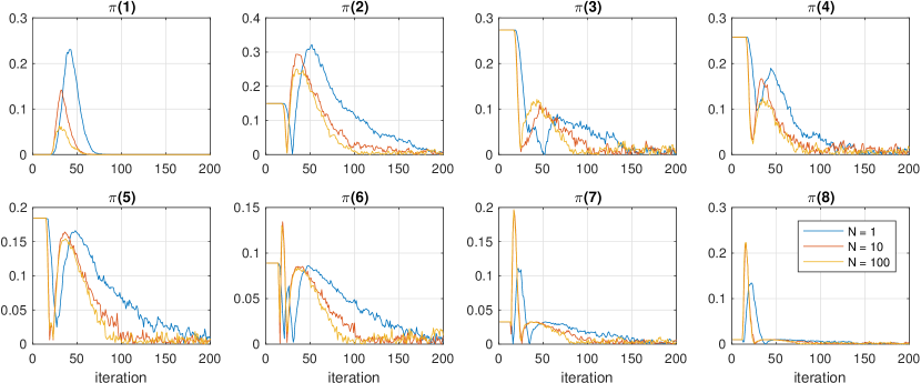
Figure 7: Estimates of time to convergence of $\mathbb{E}_{x_{0}}^{N}\big{[}f_{m}(X_{i})\big{]}$ to $\pi(m)$ for $N=1,10,100$.

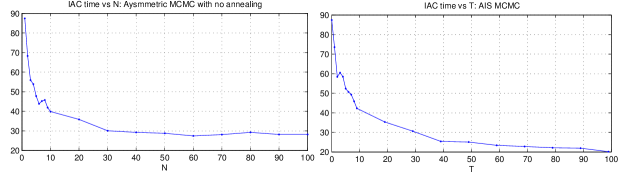
Figure 8: Left: IAC for $m$ vs number of particles $N=1,2,\ldots,10,20,\ldots,100$ with $T=0$. Right: IAC for $m$ vs number of particles $T=0,1,2,\ldots,10,20,\ldots,100$ with $N=1$.

5 State-space models: SMC and cSMC within MHAAR

In Section 4 we have shown how the generic MHAAR strategy which consists of averaging independent estimates of the acceptance ratio could be helpful in the context of inference in state-space models. Here we present an alternative where dependent estimates arising from a single conditional SMC algorithm can be averaged in order to improve performance.

5.1 State-space models and cSMC

In its simplest form, a state-space model is comprised of a latent Markov chain $\{Z_{t};t\geq 1\}$ taking its values in some measurable space $(\mathsf{Z},\mathcal{Z})$ and observations $\{Y_{t};t\geq 1\}$ taking values in $(\mathsf{Y},\mathcal{Y})$. The latent process has initial probability with density $\mu_{\theta}(z_{1})$ and transition density $f_{\theta}(z_{t-1},z_{t})$, dependent on a parameter $\theta\in\Theta\subset\mathbb{R}^{d_{\theta}}$. An observation at time $t$ is assumed conditionally independent of all other random variables given $Z_{t}=z_{t}$ and its conditional observation density is $g_{\theta}(z_{t},y_{t})$. The corresponding joint density of the latent and observed variables up to time $T$ is

$$p_{\theta}(z_{1:T},y_{1:T})=\mu_{\theta}(z_{1})\prod_{t=2}^{T}f_{\theta}(z_{t-1},z_{t})\prod_{t=1}^{T}g_{\theta}(z_{t},y_{t}),$$ (42)

from which the likelihood function associated to the observations $y_{1:T}$ can be obtained

$$l_{\theta}(y_{1:T}):=\int_{\mathsf{X}^{T}}p_{\theta}(z_{1:T},y_{1:T}){\rm d}z_{1:T}.$$ (43)

Note that the densities $f_{\theta}$ and $g_{\theta}$ could also depend on $t$, at the expense of notational complications, and that $T$ is here the time horizon of the time series and should not be confused with the number of intermediate steps in AIS in the previous sections. We allow this abuse of notation since there are no intermediate steps involved in the methodology for HMMs developed in this paper.

In order to go back to our generic notation, we let $z=z_{1:T}$ and $y=y_{1:T}$. With a prior distribution $\eta(\mathrm{d}\theta)$ on $\theta$ with density $\eta(\theta)$, the joint posterior $\pi(\mathrm{d}(\theta,z))$ has the density

$$\pi(\theta,z)\propto\eta(\theta)p_{\theta}(z,y)$$

so that $\pi(\theta)\propto\eta(\theta)\ell_{\theta}(y)$ and $\pi_{\theta}(z):=p_{\theta}(z\mid y)=p_{\theta}(z,y)/\ell_{\theta}(y)$.

The conditional sequential Monte Carlo (cSMC) algorithm for this state-space model is given in Algorithm 6, where particles are initialised using distribution $h_{\theta}(\cdot)$ on $\mathsf{(Z},\mathcal{Z})$ at time $1$ and propagated at times $t>1$ using the transition kernel $H_{\theta}(\cdot,\cdot)$ on $\mathsf{(Z},\mathcal{Z})$. The cSMC algorithm is an MCMC transition probability, akin to particle filters, particularly well suited to sampling from $\pi_{\theta}(\mathrm{d}z)$ Andrieu et al. (2010). It was recently shown in Lindsten and Schön (2012) that cSMC with backward sampling Whiteley (2010) can be used efficiently as part of a more elaborate Metropolis-within-Particle Gibbs algorithm in order to sample from the posterior distribution $\pi(\mathrm{d}(\theta,z))$; see Algorithm 7.

1

Input: Number of particles $M$, parameter $\theta$, current sample $z$

2

Output: Particles $\zeta=\zeta_{1:T}^{(1:M)}$, new sample $z^{\prime}$

3

4Set $\zeta_{1}^{(1)}=z_{1}$.

5for  $i=2,\ldots,M$ do

6      

7      Sample $\zeta_{1}^{(i)}\sim h_{\theta}(\cdot)$.

8       Compute $w_{1}^{(i)}=\mu_{\theta}\big{(}\zeta_{1}^{(i)}\big{)}g_{\theta}\big{(}\zeta_{1}^{(i)},y_{1}\big{)}/h_{\theta}\big{(}\zeta_{1}^{(i)}\big{)}$.

9

10for  $t=2,\ldots,T$ do

11      

12      Set $\zeta_{t}^{(1)}=z_{t}$.

13      for  $i=2,\ldots,M$ do

14            

15            Sample $a_{t-1}^{(i)}\sim\mathcal{P}\big{(}w_{t-1}^{(1)},\ldots,w_{t-1}^{(M)}\big{)}$ and $\zeta_{t}^{(i)}\sim H_{\theta}\big{(}\zeta_{t-1}^{(a_{t-1}^{(i)})},\cdot\big{)}$.

16             Compute $w_{t}^{(i)}=f_{\theta}\big{(}\zeta_{t-1}^{(a_{t-1}^{(i)})},\zeta_{t}^{(i)}\big{)}g_{\theta}\big{(}\zeta_{t}^{(i)},y_{t}\big{)}/H_{\theta}\big{(}\zeta_{t-1}^{(a_{t-1}^{(i)})},\zeta_{t}^{(i)}\big{)}$.

17      

18

19Sample $k_{T}\sim\mathcal{P}\big{(}w_{T}^{(1)},\ldots,w_{T}^{(M)}\big{)}$ and set $z^{\prime}_{T}=\zeta_{T}^{(k_{T})}$.

20for  $t=T-1,\ldots,1$ do

21      

22      for  $i=1,\ldots,M$ do

23            

24            Compute $\tilde{w}_{t}^{(i)}=w_{t}^{(i)}f_{\theta}\big{(}\zeta_{t}^{(i)},\zeta_{t+1}^{(k_{t+1})}\big{)}$.

25      

26      Sample $k_{t}\sim\mathcal{P}\big{(}\tilde{w}_{t}^{(1)},\ldots,\tilde{w}_{t}^{(M)}\big{)}$ and set $z^{\prime}_{t}=\zeta_{t}^{(k_{t})}$.

27

28

return $\zeta=\zeta_{1:T}^{(1:N)}$ and $z^{\prime}=z^{\prime}_{1:T}$.

Algorithm 6 $\mathrm{cSMC}\big{(}M,\theta,z\big{)}$

1

Input: Current sample $X_{n}=(\theta,z)$

2

Output: New sample $X_{n+1}$

3

4Sample $z^{\prime}\sim\mathrm{cSMC}\big{(}M,\theta,z\big{)}$.

5 Sample $\theta^{\prime}\sim q(\theta,\cdot)$.

Return $X_{n+1}=(\theta^{\prime},z^{\prime})$ with probability

$$\min\left\{1,\frac{\eta(\theta^{\prime})p_{\theta^{\prime}}(z,y)q(\theta^{\prime},\theta)}{\eta(\theta)p_{\theta}(z,y)q(\theta,\theta^{\prime})}\right\};$$ (44)

otherwise return $X_{n+1}=(\theta,z^{\prime})$.

Algorithm 7 Metropolis-within-particle Gibbs

Retaining one path from the $T\times M$ samples in the cSMC algorithm involved in Algorithm 7 may seem to be wasteful, and a natural idea is whether it is possible to make use of multiple, or even use all possible, trajectories and average out the corresponding acceptance ratios (44). We show that this is indeed possible with Algorithms 8 and 9 in the next section. We then show that these schemes improve performance at a cost which can be negligible, in particular when a parallel computing architecture is available. In order to avoid notational overload we postpone the justification of the algorithms to Appendix C. Algorithms 8 and 9 are alternative to the recently developed method

5.2 MHAAR with cSMC for state-space models

The law of the indices $\mathbf{k}:=(k_{1},\ldots,k_{T})$ drawn in the backward sampling step in Algorithm 6 (lines 6-6) conditional upon $\zeta=\zeta_{1:T}^{(1:M)}$ is given by

$$\phi_{\theta}(\mathbf{k}\mid\zeta):=\frac{w_{T}(\zeta_{T}^{(k_{T})})}{\sum_{i=1}^{M}w_{T}(\zeta_{T}^{(i)})}\prod_{t=1}^{T-1}\frac{w_{t}(\zeta_{t}^{(k_{t})})f_{\theta}(\zeta_{t}^{(k_{t})},\zeta_{t+1}^{(k_{t+1})})}{\sum_{i=1}^{M}w_{t}(\zeta_{t}^{(i)})f_{\theta}(\zeta_{t}^{(i)},\zeta_{t+1}^{(k_{t+1})})}.$$

We introduce the Markov kernel which corresponds to the sampling of a trajectory $z$ with backward-sampling, conditional upon $\zeta$,

$$\check{\Phi}_{\theta}(\zeta,{\rm d}z)=\sum_{k\in[M]^{T}}\phi_{\theta}(\mathbf{k}|\zeta)\delta_{\zeta^{(k)}}({\rm d}z),$$

where we define $[M]=\{1,\ldots,M\}$ and $\zeta^{(\mathbf{k})}:=(\zeta_{1}^{(k_{1})},\ldots,\zeta_{T}^{(k_{T})})$. Further, for any $\theta,\theta^{\prime},\tilde{\theta}\in\Theta$, and $z,z^{\prime}\in\mathsf{Z}^{T}$, define

$$\mathring{r}_{z,z^{\prime}}(\theta,\theta^{\prime};\tilde{\theta})=\frac{q(\theta^{\prime},\theta)\eta(\theta^{\prime})p_{\theta^{\prime}}(z^{\prime},y)p_{\tilde{\theta}}(z,y)}{q(\theta,\theta^{\prime})\eta(\theta)p_{\tilde{\theta}}(z^{\prime},y)p_{\theta}(z,y)}.$$ (45)

In the following, we show that it is possible to construct unbiased estimators of $r(\theta,\theta^{\prime})$ using cSMC, provided we have a random sample $z\sim\pi_{\theta}(\cdot)$. Specifically, this is achieved as the expected value of $\mathring{r}_{z,\zeta^{(\mathbf{k})}}(\theta,\theta^{\prime};\tilde{\theta})$ with respect to the backward sampling distribution on $\mathbf{k}$,

$$\mathring{r}_{z,\zeta}(\theta,\theta^{\prime};\tilde{\theta}):=\sum_{\mathbf{k}\in[M]^{T}}\phi_{\tilde{\theta}}(\mathbf{k}|\zeta)\mathring{r}_{z,\zeta^{(\mathbf{k})}}(\theta,\theta^{\prime};\tilde{\theta}).$$ (46)

Theorem 3.

For $\theta,\theta^{\prime},\tilde{\theta}\in\Theta$ and any $M\geq 1$, let $z\sim\pi_{\theta}(\cdot)$, $\zeta|z\sim\mathrm{cSMC}(M,\tilde{\theta},z)$ be the generated particles from the cSMC algorithm targeting $\pi_{\tilde{\theta}}(\cdot)$ with $M$ particles, conditioned on $z$. Then, $\mathring{r}_{z,\zeta}(\theta,\theta^{\prime};\tilde{\theta})$ is an unbiased estimator of $r(\theta,\theta^{\prime})$.

Theorem 3 is original to the best of our knowledge and we find it interesting in several aspects. Firstly, unlike the estimator in Metropolis-within-Particle Gibbs (Algorithm 7), the estimators in Theorem 3 use all possible paths from the particles generated by the cSMC. Also, with a slight modification one can similarly obtain unbiased estimators for $\pi(\theta^{\prime})/\pi(\theta)$ which is in some applications of primary interest. The theorem is derived from Del Moral et al. (2010, Theorem 5.2) and the results in Andrieu et al. (2010) relating the laws of cSMC and SMC. The proof of the theorem is left to Appendix C.

In particular, Theorem 3 motivates us to design an asymmetric MCMC algorithm which uses the unbiased estimator mentioned in the theorem in its acceptance ratios. We present Algorithm 8 that is developed with this motivation. The algorithm requires a pair of functions $\tilde{\theta}_{1}:\Theta^{2}\rightarrow\Theta$ and $\tilde{\theta}_{2}:\Theta^{2}\rightarrow\Theta$ that satisfy $\tilde{\theta}_{1}(\theta,\theta^{\prime})=\tilde{\theta}_{2}(\theta^{\prime},\theta)$, in order to determine the intermediate parameter value at which cSMC is run.

1

2

Input: Current sample $X_{n}=(\theta,z),$ number of particles $M\geq 1$

3

Output: New sample $X_{n+1}$

4

5Sample $\theta^{\prime}\sim q(\theta,\cdot)$ and $v\sim\mathcal{U}(0,1)$

6 if  $v\leq 1/2$  then

7      

8      Set $\tilde{\theta}=\tilde{\theta}_{1}(\theta,\theta^{\prime})$.

9       Run a cSMC$(M,\tilde{\theta},z)$ targeting $\pi_{\tilde{\theta}}$ conditional on $z$ to obtain $\zeta$.

10       Sample $\mathbf{k}=(k_{1},\ldots,k_{T})$ with probability $\frac{\phi_{\tilde{\theta}}(\mathbf{k}|\zeta)\mathring{r}_{z,\zeta^{(\mathbf{k})}}(\theta,\theta^{\prime};\tilde{\theta})}{\sum_{\mathbf{l}\in[M]^{T}}\phi_{\tilde{\theta}}(\mathbf{l}|\zeta)\mathring{r}_{z,\zeta^{(\mathbf{l})}}(\theta,\theta^{\prime};\tilde{\theta})}$ and set $z^{\prime}=\zeta^{(\mathbf{k})}$.

11       Set $X_{n+1}=(\theta^{\prime},z^{\prime})$ with probability $\min\{1,\mathring{r}_{z,\zeta}(\theta,\theta^{\prime};\tilde{\theta})\}$; otherwise reject the proposal and set $X_{n+1}=(\theta,z)$.

12else

13      

14      Set $\tilde{\theta}=\tilde{\theta}_{2}(\theta,\theta^{\prime})$.

15       Run a ${\rm cSMC}(M,\tilde{\theta},z)$ targeting $\pi_{\tilde{\theta}}$ conditional on $u^{(1)}=z$ to obtain $\zeta.$

16       Sample $\mathbf{k}=(k_{1},\ldots,k_{T})$ with probability $\phi_{\tilde{\theta}}(\mathbf{k}|\zeta)$ and set $z^{\prime}=\zeta^{(\mathbf{k})}$.

17       Set $X_{n+1}=(\theta^{\prime},z^{\prime})$ with probability $\min\{1,1/\mathring{r}_{z^{\prime},\zeta}(\theta^{\prime},\theta;\tilde{\theta})\}$; otherwise reject the proposal and set $X_{n+1}=(\theta,z)$.

Algorithm 8 MHAAR for state-space models with cSMC-based estimator of the likelihood ratio

The proof that Algorithm 8 is reversible is established in Appendix C.2. The proof has two interesting by-products: (i) An alternative proof of Theorem 3, and (ii) another unbiased estimate of $r(\theta,\theta^{\prime})$ that uses all possible paths that can be constructed from the particles generated by a cSMC, which is stated in the following corollary.

Corollary 1.

For $\theta,\theta^{\prime},\tilde{\theta}\in\Theta$ and any $M\geq 1$, let $z\sim\pi_{\theta}(\cdot)$, $\zeta|z\sim{\rm cSMC}(M,\tilde{\theta},z)$ be the generated particles from the cSMC algorithm with $M$ particles at $\tilde{\theta}$ conditioned on $z$, and $z^{\prime}|\zeta\sim\check{\Phi}_{\tilde{\theta}}(\zeta,\cdot)$. Then, $1/\mathring{r}_{z^{\prime},\zeta}(\theta^{\prime},\theta,\tilde{\theta})$ is an unbiased estimator of $r(\theta,\theta^{\prime}).$

5.3 Reduced computational cost via subsampling

The computations needed to implement Algorithm 8 can be performed with a complexity of $\mathcal{O}(M^{2}T)$ upon observing that the unnormalised probability can be written as

$$\phi_{\tilde{\theta}}(\mathbf{k}|\zeta)\mathring{r}_{z,\zeta^{(\mathbf{k})}}(\theta,\theta^{\prime};\tilde{\theta})=:\kappa_{z,\zeta}(\mathbf{k})=\kappa_{z,\zeta,1}(k_{1})\prod_{t=2}^{T}\kappa_{z,\zeta,t}(k_{t-1},k_{t})$$

for an appropriate choice for the functions $\kappa_{z,\zeta,t}$. Indeed, the expression above implies that computation of $\mathring{r}_{z,\zeta}(\theta,\theta^{\prime};\tilde{\theta})=\sum_{\mathbf{k}\in[M]^{T}}\kappa_{z,\zeta}(\mathbf{k})$ can be performed by a sum-product algorithm and sampling $\mathbf{k}$ with probability proportional to $\kappa_{z,\zeta}(\mathbf{k})$ can be performed with a forward-filtering backward-sampling algorithm. However, $\mathcal{O}(M^{2}T)$ can still be overwhelming, especially when $M$ is large.

In the following, we introduce a computationally less demanding version of Algorithm 8 which uses a subsampled version of (46) obtained from $N$ paths drawn using backward sampling and still preserves reversibility. Letting $\mathfrak{u}=(u^{(1)},\ldots,u^{(N)})\in\mathsf{Z}^{TN}$ , consider

$$\mathring{r}_{z,\mathfrak{u}}^{N}(\theta,\theta^{\prime};\tilde{\theta})=\frac{1}{N}\sum_{i=1}^{N}\mathring{r}_{z,u^{(i)}}(\theta,\theta^{\prime};\tilde{\theta}),$$

which is an unbiased estimator of (46) when $u^{(1)},\ldots,u^{(N)}\overset{{\rm iid}}{\sim}\check{\Phi}(\zeta,\cdot)$. In Algorithm 9 we present the multiple paths BS-cSMC asymmetric MCMC algorithm which uses $\mathring{r}_{z,\mathfrak{u}}^{N}(\theta,\theta^{\prime};\tilde{\theta})$, but still targets $\pi(\mathrm{d}(\theta,z))$, as desired. The computational complexity of this algorithm is $\mathcal{\mathcal{O}}(NMT)$ per iteration instead of $\mathcal{O}(M^{2}T)$; moreover, sampling $N$ paths can be parallelised. Reversibility of the algorithm with respect to $\pi(\mathrm{d}(\theta,z))$ is proved in Appendix C.2.

1

Input: Current sample $X_{n}=(\theta,z)$, number of particles $M\geq 1$, number of backward paths $N\geq 1$

2

Output: New sample $X_{n+1}$

3

4Sample $\theta^{\prime}\sim q(\theta,\cdot)$ and $v\sim\mathcal{U}(0,1)$.

5 if $v\leq 1/2$ then

6      

7      Set $\tilde{\theta}=\tilde{\theta}_{1}(\theta,\theta^{\prime})$.

8       Run a ${\rm cSMC}(M,\tilde{\theta},z)$ to obtain the particles $\zeta$.

9       Draw $N$ paths with backward sampling, $u^{(1)},\ldots,u^{(N)}\overset{{\rm iid}}{\sim}\check{\Phi}_{\tilde{\theta}}(\zeta,\cdot)$.

10       Sample $k\sim\mathcal{P}\big{(}\mathring{r}_{z,u^{(1)}}(\theta,\theta^{\prime};\tilde{\theta}),\ldots,\mathring{r}_{z,u^{(N)}}(\theta,\theta^{\prime};\tilde{\theta})\big{)}$ and set $z^{\prime}=u^{(k)}$.

11       Set $X_{n+1}=(\theta^{\prime},z^{\prime})$ with probability $\min\{1,\mathring{r}_{z,\mathfrak{u}}^{N}(\theta,\theta^{\prime};\tilde{\theta})\}$; otherwise reject and set $X_{n+1}=(\theta,z)$.

12else

13      

14      Set $\tilde{\theta}=\tilde{\theta}_{2}(\theta,\theta^{\prime})$.

15       Sample $k$ uniformly from $\{1,\ldots,N\}$ and set $u^{(k)}=z$.

16       Run a ${\rm cSMC}(M,\tilde{\theta},z)$ to obtain particles $\zeta$.

17       Draw $N$ paths with backward sampling $u^{(1)},\ldots,u^{(k-1)},z^{\prime},u^{(k+1)},\ldots,u^{(N)}\overset{{\rm iid}}{\sim}\check{\Phi}_{\tilde{\theta}}(\zeta,\cdot)$.

18       Set $X_{n+1}=(\theta^{\prime},z^{\prime})$ with probability $\min\{1,1/\mathring{r}_{z^{\prime},\mathfrak{u}}^{N}(\theta^{\prime},\theta;\tilde{\theta})\}$; otherwise reject and set $X_{n+1}=(\theta,z)$.

Algorithm 9 MHAAR for state-space models with cSMC-based estimator of the likelihood ratio - with reduced computation via subsampling

Example 9.

We consider the non-linear state-space of Example 7 for the same set-up. We conducted experiments similar to those of Example 8, but using this time Algorithm 9 instead, for $N=1$, $N=10$, $N=100$ and $M=150$ particles. The intermediate distribution used was similar, as were the various proposal distributions. The results for convergence and IAC times are shown in Figures 9 and 10 where the results from Example 7 are repeated in order to ease comparison. (Note that, assuming perfect parallelisation and that the computation time of cSMC is proportional to the number of particles, Algorithm 9 with $M=150$ particles and Algorithm 4 with $M=100$ particles are equally costly. This is because of the non-parallelisable part of $Q_{2}$ of Algorithm 4.)

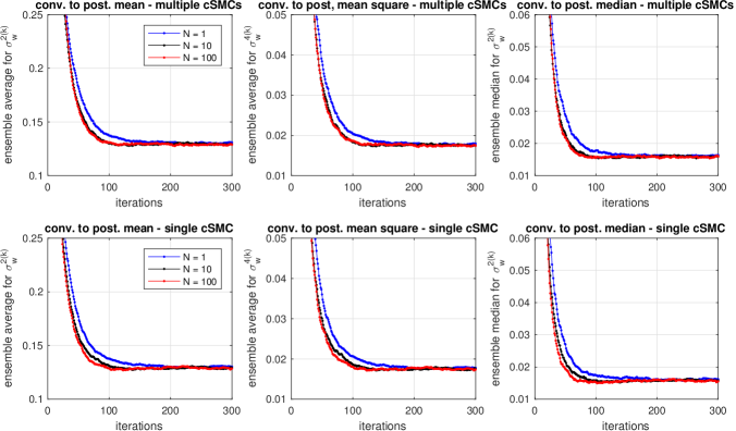
Figure 9: Convergence results for $\theta=(\sigma_{v}^{2},\sigma_{w}^{2})$ vs $N$ in Algorithm 9 in comparison with Algorithm 4.

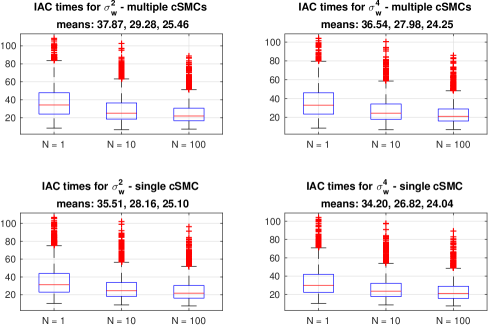
Figure 10: IAC times for $\theta=(\sigma_{v}^{2},\sigma_{w}^{2})$ vs $N$ in Algorithm 9 in comparison with Algorithm 4.

Example 10.

In this experiment, the true parameters are $\sigma_{v}^{2}=10$ and $\sigma_{w}^{2}=1$ and the data size is $T=500$. The prior and proposal parameters are the same as the previous example. We ran Metropolis-within-Particle Gibbs of Lindsten and Schön (2012) in Algorithm 7. Number of particles used in the cSMC moves is $M=100$. For each configuration, $200$ Monte Carlo runs for 100000 iterations are performed and the summary of the estimated IAC values from each run is reported in Figure 11. One can see that increasing the number of paths improves the results. However, the amount of improvement (at least for this seemingly not very challenging model) vanishes quickly after $N=10$; this is the reason we did not find necessary to look at the performance of Algorithm 8 for this example. In addition, the results suggest that the scenario $N=1$ seems useful in that the algorithm can beat Metropolis-within-Particle Gibbs for the same order of computation. Note that the $N=1$ case is also a recent algorithm, firstly proposed and analysed in Yıldırım et al. (2017), with detailed comparisons with Metropolis-within-Particle Gibbs.

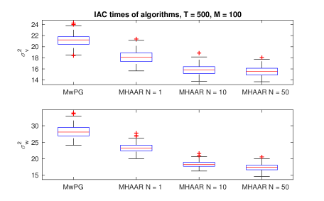
Figure 11: IAC for $\theta=(\sigma_{v}^{2},\sigma_{w}^{2})$ vs $N$ in Algorithm 9 compared to Metropolis-within-Particle Gibbs (MwPG) in Algorithm 7.

6 Discussion

In this paper, we exploit the ability to use more than one proposal scheme within a MH update. We derive several useful MHAAR algorithms that enable averaging multiple estimates of acceptance ratios, which would not be valid by using a standard single proposal MH update. The framework of MHAAR is rather general and provides a generic way of improving performance of MH update based algorithm for a wide range of problems. This is illustrated with doubly intractable models, general latent variable models, trans-dimensional models, and general state-space models. Although relevant in specific scenarios involving computations on serial machines, MHAAR algorithms are particularly useful when implemented on a parallel architecture since the computation required to have an average acceptance ratio estimate can largely be parallelised. In particular our experiments demonstrate significant reduction of the burn in period required to reach equilibrium, an issue for which very few generic approaches exist currently.

6.1 Using SMC based estimators for the acceptance ratio

More broadly the framework of using asymmetric acceptance ratios allows us to exploit even more general ratios of probabilities and plug them into MCMCs. For example, a non-trivial interesting generalisation of the algorithms presented earlier is possible by replacing AIS with SMC. The generalisation is relevant when annealing is used, i.e. $T>0$ and it is available for both the scenario $\pi(x)=\pi(\theta)$ and $\pi(x)=\pi(\theta,z)$. Notice that in Algorithms 2 to 4, the acceptance ratios of the asymmetric MCMC algorithm contain the factor

$$\frac{1}{N}\sum_{i=1}^{N}\prod_{t=0}^{T}\frac{f_{\theta,\theta^{\prime},t+1}(u_{t}^{(i)})}{f_{\theta,\theta^{\prime},t}(u_{t}^{(i)})}.$$

This average actually serves as an AIS estimator of the ratio of the normalising constants of the unnormalised densities $f_{\theta,\theta^{\prime},0}$ and $f_{\theta,\theta^{\prime},T+1}$ of the initial and the last densities used in annealing. For doubly intractable models, this quantity is $C_{\theta}/C_{\theta^{\prime}}$, whereas in latent variable models, it is $\pi(\theta^{\prime})/\pi(\theta)$. Although SMC is a well known alternative to AIS in estimating this ratio unbiasedly (Del Moral et al., 2006), it is not obvious whether or how we can substitute SMC for AIS in proposal kernels $Q_{1}$ and $Q_{2}$ and still preserve the detailed balance of the overall MCMC kernel with respect to $\pi$. It turns out that this is possible by using a SMC in $Q_{1}$ and a series of backward kernels followed by a cSMC in $Q_{2}$. For interested readers, we present $Q_{1}$ and $Q_{2}$ with the corresponding acceptance ratios, and the resulting algorithm in Appendix D.

6.2 Links to non-reversible algorithms

There has been recent interest in extending existing MCMC algorithms, especially those based on MH, to algorithms having non-reversible Markov chains preserving $\pi$ as their invariant distribution. The motivation behind such algorithms is the desire to design proposals based on the acceptance-rejection information of the previous iterations so that the space $\mathsf{X}$ is explored more efficiently. For example, it may be desirable to have a MH based Markov chain that moves in a certain direction as long as the proposed values in that direction are accepted. In case of rejection, the direction of the proposal is altered and the Markov chain is made to choose a new direction until the next rejection.

These non-reversible MH algorithms can be interpreted as using acceptance ratios involving two different proposal mechanism (e.g. for different directions). Using two different proposals is inherent to our MHAAR algorithms, and we briefly show how MHAAR algorithms can be turned into non-reversible MCMC. Consider one pair of such proposal mechanisms $Q_{1}(x,\mathrm{d}(y,u))$ and $Q_{2}(x,\mathrm{d}(y,u))$ as considered throughout this paper. The acceptance ratios involved are denoted $r_{1,u}(x,y)$ and $r_{2,u}(x,y)=1/r_{1,u}(y,x)$, depending no whether $Q_{1}$ or $Q_{2}$ is on the numerator or denominator. The non-reversible algorithm described in Algorithm 10 targets the extended distribution $\pi(\mathrm{d}(x,a)):=\pi(\mathrm{d}x)\frac{1}{2}$, where $a\in\{1,2\}$ and whose marginal is $\pi(\mathrm{d}x)$ as desired, and generates realisations $\{\big{(}X_{n},A_{n}\big{)}\in\mathsf{X}\times\{1,2\},n\geq 1\}$ where $A_{n}$ indicates which of $Q_{1}$ or $Q_{2}$ is to be used at iteration $n+1$.

1

Input: Current sample and proposal state $X_{n}=x$, $A_{n}=a$

2

Output: New sample and proposal state $X_{n+1}$, $A_{n+1}$

3

4Sample $(y,u)\sim Q_{a}(x,\cdot)$

Set $(X_{n+1},A_{n+1})=(x^{\prime},a)$ with probability $\min\{1,r_{a,u}(x,y)\}$; otherwise reject and set $(X_{n+1},A_{n+1})=(x,3-a)$.

Algorithm 10 Non-reversible MHAAR

One iteration of the algorithm is a composition of two reversible moves with respect to $\pi(\mathrm{d}(x,a))$: Given $(x,a)$, the first move consists of proposing $y,a^{\prime}$ (and $u$) from $Q_{a}(x,\mathrm{d}(y,u))\mathbb{I}_{3-a}(a^{\prime})$, accepting-rejecting with probability $\min\{1,r_{a,u}(x,y)\}$, which is the corresponding asymmetric acceptance probability for $\pi(\mathrm{d}(x,a))$. The second move simply switches the $a$-component: $a\rightarrow 3-a$, which is reversible. We do not investigate this further here.

7 Acknowledgements

CA and SY acknowledge support from EPSRC “Intractable Likelihood: New Challenges from Modern Applications (ILike)” (EP/K014463/1) and the Isaac Newton Institute for Mathematical Sciences, Cambridge, for support and hospitality during the programme “Scalable inference; statistical, algorithmic, computational aspects” where this manuscript was finalised (EPSRC grant EP/K032208/1). AD acknowledges support from EPSRC EP/K000276/1. NC is partially supported by a grant from the French National Research Agency (ANR) as part of program ANR-11-LABEX- 0047. The authors would also like to thank Nick Whiteley for useful discussions.

Appendix A A general framework for PMR and MHAAR algorithms

Assume $\pi$ is a probability distribution defined on the measurable space $(\mathsf{X},\mathcal{X})$ and let $Q_{1}(\cdot,\cdot)$ and $Q_{2}(\cdot,\cdot)$ be a pair of proposal kernels $Q_{1}(\cdot,\cdot),Q_{2}(\cdot,\cdot)\colon\mathsf{X}\times(\mathcal{U}\otimes\mathcal{X})\rightarrow[0,1]$, where $\mathcal{U}$ is a sigma-algebra corresponding to an auxiliary random variable $u$ defined on a measurable space $(\mathsf{U},\mathcal{U})$. This variable may or may not be present, and is for example ignored in the introductory Section 1.3. We first follow Tierney [1998] (in particular his treatment of Green [1995]’s framework) and introduce the measure

$$\nu_{i}\big{(}{\rm d}(x,y,u)\big{)}: =\pi({\rm d}x)Q_{i}(x,{\rm d}(y,u))+\pi({\rm d}y)Q_{3-i}(y,{\rm d}(x,u))$$

and for $i\in\{1,2\}$ the densities $\eta_{i}(x,y,u):={\rm d}(\pi\otimes Q_{i})/{\rm d}\nu_{i}$ for $(x,y,u)\in\mathsf{X}^{2}\times\mathsf{U}$. Now define the measurable set

$$\mathsf{S}:=\big{\{}(x,y,u)\in\mathsf{X}^{2}\times\mathsf{U}\colon\eta_{1}(x,y,u)>0\text{ and }\eta_{2}(y,x,u)>0\big{\}}$$ (47)

and let, for $i\in\{1,2\}$

$$r_{i,u}(x,y):=\begin{cases}\eta_{3-i}(y,x,u)/\eta_{i}(x,y,u)&\text{ for }(x,y,u)\in\mathsf{S},\\ 0&\text{otherwise}.\end{cases}$$

For ease of exposition, throughout the rest of the paper we may use the notation

$$\frac{\pi({\rm d}y)Q_{3-i}(y,{\rm d}(x,u))}{\pi({\rm d}x)Q_{i}(x,{\rm d}(y,u))}=:r_{i,u}(x,y),$$

which should not lead to any confusion. Further, for $x\in\mathsf{X}$, we define the rejection probabilities

$$\rho_{i}(x):=1-\int_{\mathsf{X}\times\mathsf{U}}Q_{i}(x,{\rm d}(y,u))\min\{1,r_{i,u}(x,y)\},\quad i=1,2.$$

In the theorem below we use the properties that for $i\in\{1,2\}$ and $(x,y)\in\mathsf{S}$ and $u\in\mathsf{U}$, then $r_{i}(x,y)r_{3-i}(y,x)=1$ and $\nu_{i}\big{(}{\rm d}(x,y,u)\big{)}=\nu_{3-i}\big{(}{\rm d}(y,x,u)\big{)}$. The following theorem serves as the basis for proving the reversibility of all of the MHAAR algorithms developed in this paper.

Theorem 4.

Consider the Markov transition kernel $\breve{P}\colon\mathsf{X}\times\mathcal{X}\rightarrow[0,1]$

$$\breve{P}(x,{\rm d}y):=\sum_{i=1}^{2}\frac{1}{2}\left[\int_{\mathsf{U}}Q_{i}(x,{\rm d}(y,u)\min\left\{1,r_{i,u}(x,y)\right\}+\delta_{x}({\rm d}y)\rho_{i}(x)\right],\quad x\in\mathsf{X}$$ (48)

then $\breve{P}$ satisfies the detailed balance for $\pi$.

Proof.

For any bounded measurable function $\phi$ on $\mathsf{X}^{2}$:

$$\int_{\mathsf{X}^{2}\times\mathsf{U}}\min\left\{1,r_{1,u}(x,y)\right\} \phi(x,y)\pi({\rm d}x)Q_{1}(x;{\rm d}(y,u))$$

$$= \int_{\mathsf{X}^{2}\times\mathsf{U}}\phi(x,y)\min\left\{1,r_{1,u}(x,y)\right\}\eta_{1}(x,y,u)\nu_{1}\big{(}{\rm d}(x,y,u)\big{)}$$

$$= \int_{\mathsf{S}}\phi(x,y)\min\left\{1,r_{1,u}(x,y)\right\}r_{2,u}(y,x)\eta_{2}(y,x,u)\nu_{1}\big{(}{\rm d}(x,y,u)\big{)}$$

$$= \int_{\mathsf{X}^{2}\times\mathsf{U}}\phi(x,y)\min\left\{1,r_{1,u}(x,y)\right\}r_{2,u}(y,x)\eta_{2}(y,x,u)\nu_{2}\big{(}{\rm d}(y,x,u)\big{)}$$

$$= \int_{\mathsf{X}^{2}\times\mathsf{U}}\phi(x,y)\min\left\{1,r_{1,u}(x,y)\right\}r_{2,u}(y,x)\pi({\rm d}y)Q_{2}(y;{\rm d}(x,u))$$

$$= \int_{\mathsf{X}^{2}\times\mathsf{U}}\phi(x,y)\min\left\{r_{2,u}(y,x),1\right\}\pi({\rm d}y)Q_{2}(y;{\rm d}(x,u)).$$

As a result for $\phi$ as above,

$$\sum_{i=1}^{2}\frac{1}{2}\int_{\mathsf{X}^{2}\times\mathsf{U}}\phi(x,y)\min\left\{1,r_{i,u}(x,y)\right\}\pi({\rm d}x)Q_{i}(x;{\rm d}(y,u))\\ =\sum_{i=1}^{2}\frac{1}{2}\int_{\mathsf{X}^{2}\times\mathsf{U}}\phi(x,y)\min\left\{1,r_{i,u}(y,x)\right\}\pi({\rm d}y)Q_{i}(y;{\rm d}(x,u)),$$

and detailed balance hence follows. ∎

The following theorem validates the use of all the PMR algorithms in this paper, specifically the algorithm corresponding to the kernel presented in (9) and the algorithms described in Propositions 1, 2 and 4.

Theorem 5.

Let $\varphi:\mathsf{U}\rightarrow\mathsf{U}$ be a measurable involution, that is such that $\varphi\circ\varphi(u)=u$ for all $u\in\mathsf{U}$ and with the set-up of Theorem 4 for a given kernel $Q_{1}(\cdot,\cdot)$, let $Q_{2}(\cdot,\cdot)$ be defined such that for any measurable $\psi\colon\mathsf{X}^{2}\times\mathsf{U}\rightarrow[-1,1]$

$$\int\psi(x,y,u)\pi({\rm d}x)Q_{2}\big{(}x,\mathrm{d}(y,u)\big{)} =\int\psi(x,y,\varphi(u))\pi({\rm d}x)Q_{1}\big{(}x,\mathrm{d}(y,u)\big{)}.$$

Then the Markov transition kernel

$$\mathring{P}(x,\mathrm{d}y)=\int_{\mathsf{U}}Q_{1}(x,\mathrm{d}(y,u))\min\left\{1,r_{1,u}(x,y)\right\}+\rho_{1}(x)\delta_{x}(\mathrm{d}y)$$

satisfies detailed balance with respect to $\pi$.

Proof.

$$\nu_{1}\big{(}{\rm d}(x,y,u)\big{)}=\nu_{2}\big{(}{\rm d}(y,x,u)\big{)}$$

First we show that

$$\int\psi(x,y,u)\nu_{1}(\mathrm{d}(x,y,u))=\int\psi(x,y,\varphi(u))\nu_{1}(\mathrm{d}(y,x,u)).$$ (49)

This is because for $\psi$ bounded and measurable

$$\int\psi(x,y,u)\nu_{1}\big{(}{\rm d}(x,y,u)\big{)} =\int\psi(x,y,u)(\pi\otimes Q_{1})\big{(}{\rm d}(x,y,u)\big{)}+\int\psi(x,y,\varphi(u))(\pi\otimes Q_{1})\big{(}{\rm d}(y,x,u)\big{)}$$

$$=\int\psi(x,y,\varphi(u))(\pi\otimes Q_{2})\big{(}{\rm d}(x,y,u)\big{)}+\int\psi(x,y,\varphi(u))(\pi\otimes Q_{1})\big{(}{\rm d}(y,x,u)\big{)}$$

$$=\int\psi(x,y,\varphi(u))\nu_{1}\big{(}{\rm d}(y,x,u)\big{)},$$

where we have used our assumption on $\pi\otimes Q_{2}$ on the first and second line, together with the fact that $\varphi$ is an involution, and the definition of $\nu_{1}$ on the last line. As a result one can establish that

$$\eta_{2}(x,y,u)=\eta_{1}(x,y,\varphi(u)).$$

Indeed, for $\psi$ bounded and measurable,

$$\int\psi(x,y,u)\eta_{2}(x,y,u)\nu_{2}\big{(}{\rm d}(x,y,u)\big{)}= \int\psi(x,y,u)\pi\otimes Q_{2}\big{(}{\rm d}(x,y,u)\big{)}$$

$$= \int\psi(x,y,\varphi(u))\pi\otimes Q_{1}\big{(}{\rm d}(x,y,u)\big{)}$$

$$= \int\psi(x,y,\varphi(u))\eta_{1}(x,y,u)\nu_{1}\big{(}{\rm d}(x,y,u)\big{)}$$

$$= \int\psi(x,y,u)\eta_{1}(x,y,\varphi(u))\nu_{1}\big{(}{\rm d}(y,x,u)\big{)}$$

$$= \int\psi(x,y,u)\eta_{1}(x,y,\varphi(u))\nu_{2}\left({\rm d}(x,y,u)\right),$$

where we have used (49) on the fourth line. Now for $\phi\colon\mathsf{X}^{2}\rightarrow[-1,1]$ measurable

$$\int_{\mathsf{X}\times\mathsf{U}\times\mathsf{X}}\phi(x,y)\min \left\{1,r_{1,u}(x,y)\right\}\pi({\rm d}x)Q_{1}(x,\mathrm{d}(y,u))$$

$$=\int_{\mathsf{S}}\phi(x,y)\min\left\{1,r_{1,u}(x,y)\right\}\frac{\eta_{1}(x,y,u)}{\eta_{1}(y,x,\varphi(u))}\eta_{1}(y,x,\varphi(u))\nu_{1}(\mathrm{d}(x,y,u))$$

$$=\int_{\mathsf{S}}\phi(x,y)\min\left\{r_{1,\varphi(u)}(y,x),1\right\}\eta_{1}(y,x,\varphi(u))\nu_{1}(\mathrm{d}(x,y,u))$$

$$=\int_{\mathsf{S}}\phi(x,y)\min\left\{r_{1,u}(y,x),1\right\}\eta_{1}(y,x,u)\nu_{1}(\mathrm{d}(y,x,u)),$$

and reversibility follows. ∎

A.1 Specialisation to two specific scenarios

Although the general framework described in Theorem 4 is quite broad, our algorithms exploit it in specific ways. In this subsection, we aim to provide some insight into the ways we exploit these ideas in this paper. Recall that we either have $x=\theta$ in the single variable case or $x=(\theta,z)$ in the scenario where the model involves latent variables. Throughout the paper, we design algorithms where both $Q_{1}(\cdot,\cdot)$ and $Q_{2}(\cdot,\cdot)$ use the same proposal distribution for $\theta^{\prime}$, that is $q(\theta,\cdot)$ and differ in the way they sample the auxiliary variables (and $z^{\prime}$ in the latent variables scenario) such that $Q_{1}(\cdot,\cdot)$ and $Q_{2}(\cdot,\cdot)$ complement each other to produce acceptance ratio estimators whose statistical properties increase with (parallelisable) computations.

A.1.1 Single variable scenario

Here we have $x=\theta$. Let $\{Q_{\theta,\theta^{\prime}}^{(1)}(\cdot)\colon\theta,\theta^{\prime}\in\Theta\}$ and $\{Q_{\theta,\theta^{\prime}}^{(2)}(\cdot)\colon\theta,\theta^{\prime}\in\Theta\}$ be two families of probability distributions defined on $(\mathsf{U,\mathcal{U}})$ and $\omega_{\theta,\theta^{\prime}}:\mathcal{\mathsf{U}}\rightarrow[0,\infty)$ satisfying the condition, for $\theta,\theta^{\prime}\in\Theta$ and $u\in\mathsf{U}$,

$$Q_{\theta^{\prime},\theta}^{(2)}(\mathrm{d}u)=Q_{\theta,\theta^{\prime}}^{(1)}(\mathrm{d}u)\omega_{\theta,\theta^{\prime}}(u),$$ (50)

so that the expected value of $\omega_{\theta,\theta^{\prime}}(\cdot)$ with respect to $Q_{\theta,\theta^{\prime}}^{(1)}(\cdot)$ (as well as the expected value of $\omega_{\theta,\theta^{\prime}}^{-1}(\cdot)$ with respect to $Q_{\theta^{\prime},\theta}^{(2)}(\cdot)$ if $\omega_{\theta,\theta^{\prime}}(\cdot)>0$) is $1$. Then the Radon-Nikodym derivative evaluated for $(\theta,u,\theta^{\prime})\in\mathsf{S}$ as defined above,

$$r_{u}(\theta,\theta^{\prime})=\frac{\pi(\mathrm{d}\theta^{\prime})q(\theta^{\prime},\mathrm{d}\theta)Q_{\theta^{\prime},\theta}^{(2)}(\mathrm{d}u)}{\pi(\mathrm{d}\theta)q(\theta,\mathrm{d}\theta^{\prime})Q_{\theta,\theta^{\prime}}^{(1)}(\mathrm{d}u)}=r(\theta,\theta^{\prime})\omega_{\theta,\theta^{\prime}}(u).$$ (51)

Note that this ratio is an unbiased estimator of the acceptance ratio of the marginal distribution, $r(\theta,\theta^{\prime})$; therefore useful algorithm can be constructed if (i) $r(\theta,\theta^{\prime})\omega_{\theta,\theta^{\prime}}(u)$ can be evaluated, and (ii) the variance of of $\omega_{\theta,\theta^{\prime}}$ can be controlled. It follows exactly from (51) and Theorem 4 that we can construct a reversible Markov kernel using acceptance ratios involving $r_{u}(\theta,\theta^{\prime})$ as in Theorem 4 with

$$Q_{1}(\theta,\mathrm{d}(\theta^{\prime},u))=q(\theta,\mathrm{d}\theta^{\prime})Q_{\theta,\theta^{\prime}}^{(1)}(\mathrm{d}u),\quad Q_{2}(\theta,\mathrm{d}(\theta^{\prime},u))=q(\theta,\mathrm{d}\theta^{\prime})Q_{\theta,\theta^{\prime}}^{(2)}(\mathrm{d}u).$$

If, in addition, for any measurable and bounded function $\phi$ we have $\int\phi(u)Q_{\theta,\theta^{\prime}}^{(2)}(\mathrm{d}u)=\int\phi\circ\varphi(u)Q_{\theta,\theta^{\prime}}^{(1)}(\mathrm{d}u)$ for some involution $\varphi$, we are precisely in the frame of the pseudo-marginal ratio algorithms discussed in Nicholls et al. [2012], whose transition kernel is given in Theorem 5.

A.1.2 Latent model scenario

Here we have $x=(\theta,z)$ with $\pi(\mathrm{d}x)=\pi(\mathrm{d}\theta)\pi_{\theta}(\mathrm{d}z)$. Let $\{Q_{\theta,\theta^{\prime},z}^{(1)}(\cdot)\colon\theta,\theta^{\prime}\in\Theta\}$ and $\{Q_{\theta,\theta^{\prime},z}^{(2)}(\cdot)\colon\theta,\theta^{\prime}\in\Theta,z\in\mathsf{Z}\}$ be two families of probability distributions defined on $(\mathsf{\mathsf{Z}\times U,\mathcal{Z}\otimes\mathcal{U}})$ and $\omega_{\theta,\theta^{\prime}}:\mathcal{\mathsf{Z}}\times\mathsf{U}\rightarrow[0,\infty)$ satisfying the condition

$$\pi_{\theta^{\prime}}(\mathrm{d}z^{\prime})Q_{\theta^{\prime},\theta,z^{\prime}}^{(2)}(\mathrm{d}(z,u))=\pi_{\theta}(\mathrm{d}z)Q_{\theta,\theta^{\prime},z}^{(1)}(\mathrm{d}(z^{\prime},u))\omega_{\theta,\theta^{\prime}}(z,u),$$

so that the expected value of $\omega_{\theta,\theta^{\prime}}(z,u)$ with respect to $\pi_{\theta}(\mathrm{d}z)Q_{\theta,\theta^{\prime},z}^{(1)}(\mathrm{d}(z^{\prime},u))$ is $1$. Just as in the single variable case, consider the Radon-Nikodym derivative again:

$$r_{u}(x,x^{\prime})=\frac{\pi(\mathrm{d}x^{\prime})q(\theta^{\prime},\mathrm{d}\theta)Q_{\theta^{\prime},\theta,z^{\prime}}^{(2)}(\mathrm{d}(z,u))}{\pi(\mathrm{d}x)q(\theta,\mathrm{d}\theta^{\prime})Q_{\theta,\theta^{\prime},z}^{(1)}(\mathrm{d}(z^{\prime},u))}=r(\theta,\theta^{\prime})\omega_{\theta,\theta^{\prime}}(z,u).$$ (52)

Note that this ratio is an unbiased estimator of the acceptance ratio of the marginal distribution, $r(\theta,\theta^{\prime})$; therefore useful a algorithm can be constructed if (i) $r(\theta,\theta^{\prime})\omega_{\theta,\theta^{\prime}}(z,u)$ can be evaluated and (ii) the variance of of $\omega_{\theta,\theta^{\prime}}$ can be controlled. We can construct a reversible Markov kernel using $Q_{1}(\cdot,\cdot)$ and $Q_{2}(\cdot,\cdot)$ as:

$$Q_{1}(x,\mathrm{d}(x^{\prime},u))=q(\theta,\mathrm{d}\theta^{\prime})Q_{\theta,\theta^{\prime},z}^{(1)}(\mathrm{d}(z^{\prime},u)),\quad Q_{2}(x,\mathrm{d}(x^{\prime},u))=q(\theta,\mathrm{d}\theta^{\prime})Q_{\theta,\theta^{\prime},z}^{(2)}(\mathrm{d}(z^{\prime},u)).$$

Similarly, if, in addition, for any bounded measurable function $\phi$ we have $\int\phi(z,u)\pi_{\theta}({\rm d}z)Q_{\theta,\theta^{\prime},z}^{(2)}(\mathrm{d}(z^{\prime},u))=\int\phi(z,\varphi(u))\pi_{\theta}({\rm d}z)Q_{\theta,\theta^{\prime},z}^{(1)}(\mathrm{d}(z^{\prime},u))$ for some some involution $\varphi\colon\mathsf{U}\rightarrow\mathsf{U}$, we can use the transition kernel given in Theorem 5 and we end up precisely in the framework of the pseudo-marginal ratio algorithms for latent variable models discussed in Section 4.

A.2 Generalisation and theoretical sub-optimality

One can be more general than having a single pair of proposal distributions and sampling them with equal probabilities. In the following, we will consider multiple pairs and sampling among proposal distributions with state-dependent probabilities. Then we will investigate the statistical properties of this scheme by comparing it to an ideal but non-implementable algorithm in terms of Peskun order. For some $m\in\mathbb{N}$ let $\{Q_{ij}(\cdot,\cdot),i,j\in\{1,\ldots,m\}\}$ be a family of proposal kernels each from $(\mathsf{X},\mathcal{X})$ to $(\mathsf{X}\times\mathsf{U},\mathcal{X}\times\mathcal{U})$ and $\{\beta_{ij}:\mathsf{X}\rightarrow[0,1],i,j\in\{1,\ldots,m\}\}$ such that for any $x\in\mathsf{X}$, $\sum_{i,j=1}^{m}\beta_{ij}(x)=1$. Define the Markov transition kernel

$$\breve{P}(x,{\rm d}y):=\sum_{i=1}^{m}\sum_{j=1}^{m}\beta_{ij}(x)\left[\int_{\mathsf{U}}Q_{ij}(x,{\rm d}(y,u))\min\left\{1,r_{ij,u}(x,y)\right\}+\delta_{x}({\rm d}y)\rho_{ij}(x)\right],\quad x\in\mathsf{X}$$ (53)

where the acceptance ratios are

$$r_{ij,u}(x,y):=\frac{\pi({\rm d}y)Q_{ji}(y,{\rm d}(x,u))}{\pi({\rm d}x)Q_{ij}(x,{\rm d}(y,u))}\frac{\beta_{ji}(y)}{\beta_{ij}(x)},\quad i,j=1,\ldots,m,$$

on some set $\mathring{\mathsf{S}}_{ij}\subset\mathsf{X}\times\mathsf{U}\times\mathsf{X}$ where the measures $\pi({\rm d}y)Q_{ji}(y,{\rm d}(x,u))$ and $\pi({\rm d}x)Q_{ij}(x,{\rm d}(y,u))$ are equivalent (see the beginning of Appendix A) and $0<\beta_{ij}(x)\beta_{ji}(y)<\infty$ and set to zero otherwise, while the rejection probabilities at $x\in\mathsf{X}$ corresponding to all the updates are given by

$$\rho_{ij}(x):=1-\int_{\mathsf{U}\times\mathsf{X}}Q_{ij}(x,{\rm d}(y,u))\min\{1,r_{ij,u}(x,y)\},\quad i,j=1,\ldots,m.$$

Reversibility of $\breve{P}$ can be proven very similarly to Theorem 4, therefore it is only stated as a corollary below.

Corollary 2.

The MHAAR algorithm with transition kernel $\breve{P}$ in (53) satisfies detailed balance for $\pi$.

The standard MH algorithm is recovered, for example, in the situation where $\beta_{11}(x)=1$. The single pair version is recovered with $\beta_{12}(x)=\beta_{21}(x)=1/2$ and $Q_{12}(\cdot,\cdot)=Q_{1}(\cdot,\cdot)$, $Q_{21}(\cdot,\cdot)=Q_{2}(\cdot,\cdot)$. Algorithm 5 corresponds to the special case where $\beta_{12}(x)+\beta_{21}(x)=1$.

The following interpretation of $\breve{P}$ points to a theoretical sub-optimality of asymmetric MCMC a careful reader may point to. Indeed, from (53), the auxiliary variable $u\in\mathsf{U}$ and the proposed value $y\in\mathsf{X}$ are sampled from

$$\breve{Q}(x,\cdot):=\sum_{i=1}^{m}\sum_{j=1}^{m}\beta_{ij}(x)Q_{ij}(x,\cdot),$$

and the proposed value is accepted with probability

$$\breve{\alpha}_{u}(x,y):=\sum_{i=1}^{m}\sum_{j=1}^{m}\frac{\beta_{ij}(x)Q_{ij}(x,{\rm d}(y,u))}{\breve{Q}(x,{\rm d}(y,u))}\min\{1,r_{ij,u}(x,y)\}.$$

Application of Jensen’s inequality shows that for $x,y\in\mathsf{X}$, $u\in\mathsf{U}$, we have

$$\breve{\alpha}_{u}(x,y) \leq\min\left\{1,\sum_{i=1}^{m}\sum_{j=1}^{m}\frac{\beta_{ij}(x)Q_{ij}(x,{\rm d}(y,u))}{\breve{Q}(x,{\rm d}(y,u))}r_{ij,u}(x,y)\right\}$$

$$=\min\left\{1,\sum_{i=1}^{m}\sum_{j=1}^{m}\frac{\beta_{ij}(x)Q_{ij}(x,{\rm d}(y,u))}{\breve{Q}(x,{\rm d}(y,u))}\frac{\beta_{ji}(y)\pi({\rm d}y)Q_{ji}(y,{\rm d}(x,u))}{\beta_{ij}(x)\pi({\rm d}x)Q_{ij}(x,{\rm d}(y,u))}\right\}$$

$$=\min\left\{1,\frac{\pi({\rm d}y)\breve{Q}(y,{\rm d}(x,u))}{\pi({\rm d}x)\breve{Q}(x,{\rm d}(y,u))}\right\}=:\alpha_{u}(x,y),$$ (54)

which is the acceptance probability of a pseudo-marginal ratio MH algorithm $\mathring{P}$ with $Q_{1}(\cdot,\cdot)=\breve{Q}(\cdot,\cdot)$ and $\varphi(u)=u$ (see Theorem 5). From Peskun’s result Tierney [1998] we deduce that for this common proposal distribution $\breve{Q}$, the update $\breve{P}$ has worse performance properties in terms of both asymptotic variance and right spectral gap than $\mathring{P}$. It is therefore natural to question the interest of updates such as $\breve{P}$. An argument already noted by Tjelmeland and Eidsvik [2004], Andrieu and Thoms [2008], is that computing the acceptance ratio in (54) is generally substantially more computationally expensive than computing $\breve{r}_{ij}(x,y)$, which may offset any theoretical advantage in practice. It may also be that defining a desirable acceptance ratio is theoretically impossible using the standard approach, or that practical evaluation of the acceptance ratio is impossible. This is the case for numerous examples, including Example 4, for which

$$\alpha_{u}(\theta,\theta^{\prime}) =r(\theta,\theta^{\prime})\frac{\big{[}\prod_{i=1}^{N}g_{\theta}(u^{(i)})/C_{\theta}\,\mathring{r}_{u^{(k)}}(\theta^{\prime},\theta)/\mathring{r}_{\mathfrak{u}}^{N}(\theta^{\prime},\theta)+N^{-1}g_{\theta}(u^{(k)})/C_{\theta}\prod_{i\neq k}g_{\theta^{\prime}}(u^{(i)})/C_{\theta^{\prime}}\big{]}}{\big{[}\prod_{i=1}^{N}g_{\theta^{\prime}}(u^{(i)})/C_{\theta^{\prime}}\,\mathring{r}_{u^{(k)}}(\theta,\theta^{\prime})/\mathring{r}_{\mathfrak{u}}^{N}(\theta,\theta^{\prime})+N^{-1}g_{\theta^{\prime}}(u^{(k)})/C_{\theta^{\prime}}\prod_{i\neq k}g_{\theta}(u^{(i)})/C_{\theta}\big{]}},$$

for $N\geq 1$ and where we note that the unknown normalising constants do not cancel.

Appendix B Justification of AIS and an extension

We provide here a short justification of the AIS of Crooks [1998], Neal [2001], as presented in Karagiannis and Andrieu [2013], and an extension of it that is useful in this paper. Here $\tau$ represents the number of intermediate distributions introduced, while $\mu_{0}$ and $\mu_{\tau+1}$ are the distributions of which we want the normalising constants as we assume that we only know them up to normalising constants i.e. we know the unnormalised distributions $\nu_{0}=\mu_{0}Z_{0}$ and $\nu_{\tau+1}=\mu_{\tau+1}Z_{\tau+1}$.

Theorem 6.

Let $\big{\{}\mu_{t},t=0,\ldots,\tau+1\big{\}}$ for some $\tau\in\mathbb{N}$ be a family of probability distributions on some measurable space $\big{(}\mathsf{E},\mathcal{E}\big{)}$ such that for $t=0,\ldots,\tau$ $\mu_{t}\gg\mu_{t+1}$. Let $\big{\{}\Pi_{t},t=1,\ldots,\tau\big{\}}$ be a family of Markov transition kernels $\Pi_{t}:\mathsf{E}\times\mathcal{E}\rightarrow[0,1]$ such that for any $t=1,\ldots,\tau$, $\Pi_{t}$ is $\mu_{t}-$reversible. Let us define the following probability distributions on $\big{(}\mathsf{E}^{\tau+1},\mathcal{E}^{\tau+1}\big{)}$, $\overleftarrow{\varPi}:=\mu_{\tau+1}\times\Pi_{\tau}\times\cdots\times\Pi_{1}$ and $\overrightarrow{\varPi}:=\mu_{0}\times\Pi_{1}\times\cdots\times\Pi_{\tau}$ for $\tau\geq 1$ and $\overleftarrow{\varPi}:=\mu_{\tau+1}$ and $\overrightarrow{\varPi}:=\mu_{0}$ for $\tau=0$. Then for any $x_{0:\tau}\in\mathsf{E}^{\tau+1}$

$$\overleftarrow{\varPi}\big{(}{\rm d}(x_{\tau},\ldots,x_{0})\big{)} =\prod_{t=0}^{\tau}\frac{\mu_{t+1}\big{(}{\rm d}x_{t}\big{)}}{\mu_{t}\big{(}{\rm d}x_{t}\big{)}}\overrightarrow{\varPi}\big{(}{\rm d}(x_{0},\ldots,x_{\tau})\big{)}.$$

Proof.

The case $\tau=0$ is direct. Assume $\tau\geq 1$, we show by induction that for any $j=1,\ldots,\tau$

$$\overleftarrow{\varPi}\big{(}{\rm d}(x_{\tau},\ldots,x_{0})\big{)}\\ =\left[\prod_{t=1}^{j}\frac{\mu_{\tau-t+2}\big{(}{\rm d}x_{\tau+1-t}\big{)}}{\mu_{\tau-t+1}\big{(}{\rm d}x_{\tau+1-t}\big{)}}\Pi_{\tau+1-t}\big{(}x_{\tau-t},{\rm d}x_{\tau-t+1}\big{)}\right]\mu_{\tau-j+1}\big{(}{\rm d}x_{\tau-j}\big{)}\prod_{t=j+1}^{\tau}\Pi_{\tau-t+1}\big{(}x_{\tau-t+1},{\rm d}x_{\tau-t}\big{)},$$

with the convention $\prod_{t=\tau+1}^{\tau}=I$. First we check the result for $j=1$

$$\overleftarrow{\varPi}\big{(}{\rm d}(x_{\tau},\ldots,x_{0})\big{)} =\mu_{\tau+1}\big{(}{\rm d}x_{\tau}\big{)}\prod_{t=1}^{\tau}\Pi_{\tau-t+1}\big{(}x_{\tau-t+1},{\rm d}x_{\tau-t}\big{)}$$

$$=\frac{\mu_{\tau+1}\big{(}{\rm d}x_{\tau}\big{)}}{\mu_{\tau}\big{(}{\rm d}x_{\tau}\big{)}}\mu_{\tau}\big{(}{\rm d}x_{\tau}\big{)}\Pi_{\tau}\big{(}x_{\tau},{\rm d}x_{\tau-1}\big{)}\prod_{t=2}^{\tau}\Pi_{\tau-t+1}\big{(}x_{\tau-t+1},{\rm d}x_{\tau-t}\big{)}$$

$$=\frac{\mu_{\tau+1}\big{(}{\rm d}x_{\tau}\big{)}}{\mu_{\tau}\big{(}{\rm d}x_{\tau}\big{)}}\mu_{\tau}\big{(}{\rm d}x_{\tau-1}\big{)}\Pi_{\tau}\big{(}x_{\tau-1},{\rm d}x_{\tau}\big{)}\prod_{t=2}^{\tau}\Pi_{\tau-t+1}\big{(}x_{\tau-t+1},{\rm d}x_{\tau-t}\big{)},$$

where we have used $\mu_{\tau}\gg\mu_{\tau+1}$ and the fact that $\Pi_{\tau}$ is $\mu_{\tau}-$reversible. Now assume the result true for some $1\leq j\leq\tau-1$ and $\tau\geq 2$, then using similar arguments as above,

$$\mu_{\tau-j+1}\big{(}{\rm d}x_{\tau-j}\big{)}\Pi_{\tau-j}\big{(}x_{\tau-j}, {\rm d}x_{\tau-j-1}\big{)}$$

$$=\frac{\mu_{\tau-j+1}\big{(}{\rm d}x_{\tau-j}\big{)}}{\mu_{\tau-j}\big{(}{\rm d}x_{\tau-j}\big{)}}\mu_{\tau-j}\big{(}{\rm d}x_{\tau-j}\big{)}\Pi_{\tau-j}\big{(}x_{\tau-j},{\rm d}x_{\tau-j-1}\big{)}$$

$$=\frac{\mu_{\tau-j+1}\big{(}{\rm d}x_{\tau-j}\big{)}}{\mu_{\tau-j}\big{(}{\rm d}x_{\tau-j}\big{)}}\mu_{\tau-j}\big{(}{\rm d}x_{\tau-j-1}\big{)}\Pi_{\tau-j}\big{(}x_{\tau-j-1},{\rm d}x_{\tau-j}\big{)},$$

from which the intermediate claim follows for $j+1$. Now for $j=\tau$ we obtain the claimed result after a change of variables $t\leftarrow\tau+1-t$ in the product. ∎

Corollary 3.

Assume that we have access to unnormalised versions of the probability distributions, say $\nu_{t}=\mu_{t}Z_{t}$. Then

$$\overleftarrow{\varPi}\big{(}{\rm d}(x_{\tau},\ldots,x_{0})\big{)}=\prod_{t=0}^{\tau}\frac{Z_{t}}{Z_{t+1}}\frac{\nu_{t+1}\big{(}{\rm d}x_{t}\big{)}}{\nu_{t}\big{(}{\rm d}x_{t}\big{)}}\overrightarrow{\varPi}\big{(}{\rm d}(x_{0},\ldots,x_{\tau})\big{)},$$

and therefore

$$\prod_{t=0}^{\tau}\frac{\nu_{t+1}\big{(}{\rm d}x_{t}\big{)}}{\nu_{t}\big{(}{\rm d}x_{t}\big{)}}\overrightarrow{\varPi}\big{(}{\rm d}(x_{0},\ldots,x_{\tau})\big{)} =\overleftarrow{\varPi}\big{(}{\rm d}(x_{\tau},\ldots,x_{0})\big{)}\prod_{t=0}^{\tau}\frac{Z_{t+1}}{Z_{t}}$$

$$=\overleftarrow{\varPi}\big{(}{\rm d}(x_{\tau},\ldots,x_{0})\big{)}\frac{Z_{\tau+1}}{Z_{0}},$$

which suggests and justifies the AIS estimator.

The following extension of the result above turns out to be of practical interest.

Theorem 7.

Let $\tau\geq 2$, $\big{\{}\mu_{t},t=1,\ldots,\tau\big{\}}$ and $\big{\{}\Pi_{t},t=2,\ldots,\tau-1\big{\}}$ be as in Theorem 6 above but assume now that $\mu_{0}$ and $\mu_{\tau+1}$ are defined on a potentially different measurable space $(\mathsf{F},\mathcal{F})$. Further let $\overrightarrow{\Pi}_{1},\overleftarrow{\Pi}_{\tau}:\mathsf{F}\times\mathcal{E}\rightarrow[0,1]$ and $\overleftarrow{\Pi}_{1},\overrightarrow{\Pi}_{\tau}:\mathsf{E}\times\mathcal{F}\rightarrow[0,1]$ be Markov kernels satisfying the following properties

$$\mu_{0}\big{(}{\rm d}x_{0}\big{)}\overrightarrow{\Pi}_{1}\big{(}x_{0},{\rm d}x_{1}\big{)}=\mu_{1}\big{(}{\rm d}x_{1}\big{)}\overleftarrow{\Pi}_{1}\big{(}x_{1},{\rm d}x_{0}\big{)},$$

and

$$\mu_{\tau}\big{(}{\rm d}x_{\tau-1}\big{)}\overrightarrow{\Pi}_{\tau}\big{(}x_{\tau-1},{\rm d}x_{\tau}\big{)}=\mu_{\tau+1}\big{(}{\rm d}x_{\tau}\big{)}\overleftarrow{\Pi}_{\tau}\big{(}x_{\tau},{\rm d}x_{\tau-1}\big{)}.$$

Define

$$\overrightarrow{\varPi}:=\mu_{0}\times\overrightarrow{\Pi}_{1}\times\Pi_{2}\cdots\times\overrightarrow{\Pi}_{\tau},$$

and

$$\overleftarrow{\varPi}:=\mu_{\tau+1}\times\overleftarrow{\Pi}_{\tau}\times\Pi_{\tau-1}\cdots\times\overleftarrow{\Pi}_{1}.$$

Then

$$\overleftarrow{\varPi}\big{(}{\rm d}(x_{\tau},\ldots,x_{0})\big{)}=\prod_{t=1}^{\tau-1}\frac{\mu_{t+1}\big{(}{\rm d}x_{t}\big{)}}{\mu_{t}\big{(}{\rm d}x_{t}\big{)}}\overrightarrow{\varPi}\big{(}{\rm d}(x_{0},\ldots,x_{\tau})\big{)}.$$

Proof.

The proof follows from manipulations similar to those of Theorem 6. We have,

$$\overleftarrow{\varPi} \big{(}{\rm d}(x_{\tau},\ldots,x_{0})\big{)}=\mu_{\tau+1}\big{(}{\rm d}x_{\tau}\big{)}\overleftarrow{\Pi}_{\tau}\big{(}x_{\tau},{\rm d}x_{\tau-1}\big{)}\left[\prod_{t=2}^{\tau-1}\Pi_{\tau-t+1}\big{(}x_{\tau-t+1},{\rm d}x_{\tau-t}\big{)}\right]\overleftarrow{\Pi}_{1}(x_{1},\mathrm{d}x_{0})$$

$$=\left[\frac{\mu_{\tau}\big{(}{\rm d}x_{\tau-1}\big{)}}{\mu_{\tau-1}\big{(}{\rm d}x_{\tau-1}\big{)}}\overrightarrow{\Pi}_{\tau}\big{(}x_{\tau-1},{\rm d}x_{\tau}\big{)}\right]\left[\mu_{\tau-1}\big{(}{\rm d}x_{\tau-1}\big{)}\prod_{t=2}^{\tau-1}\Pi_{t}\big{(}x_{t},{\rm d}x_{t-1}\big{)}\right]\overleftarrow{\Pi}_{1}(x_{1},\mathrm{d}x_{0})$$

$$=\left[\frac{\mu_{\tau}\big{(}{\rm d}x_{\tau-1}\big{)}}{\mu_{\tau-1}\big{(}{\rm d}x_{\tau-1}\big{)}}\overrightarrow{\Pi}_{\tau}\big{(}x_{\tau-1},{\rm d}x_{\tau}\big{)}\right]\left[\left\{\prod_{t=2}^{\tau-1}\frac{\mu_{t}\big{(}{\rm d}x_{t-1}\big{)}}{\mu_{t-1}\big{(}{\rm d}x_{t-1}\big{)}}\right\}\prod_{t=2}^{\tau-1}\Pi_{t}\big{(}x_{t-1},{\rm d}x_{t}\big{)}\mu_{1}\big{(}{\rm d}x_{1}\big{)}\right]\overleftarrow{\Pi}_{1}(x_{1},\mathrm{d}x_{0})$$

$$=\left\{\prod_{t=1}^{\tau-1}\frac{\mu_{t+1}\big{(}{\rm d}x_{t}\big{)}}{\mu_{t}\big{(}{\rm d}x_{t}\big{)}}\right\}\left[\overrightarrow{\Pi}_{\tau}\big{(}x_{\tau-1},{\rm d}x_{\tau}\big{)}\prod_{t=2}^{\tau-1}\Pi_{\tau-t+1}\big{(}x_{\tau-t},{\rm d}x_{\tau-t+1}\big{)}\overrightarrow{\Pi}_{1}\big{(}x_{0},{\rm d}x_{1}\big{)}\mu_{0}\big{(}{\rm d}x_{0}\big{)}\right]$$

$$=\left\{\prod_{t=1}^{\tau-1}\frac{\mu_{t+1}\big{(}{\rm d}x_{t}\big{)}}{\mu_{t}\big{(}{\rm d}x_{t}\big{)}}\right\}\overrightarrow{\varPi}(\mathrm{d}(x_{0},\ldots,x_{\tau}))$$

where on the second and fourth line we have used the two conditions on the arrowed kernels, and the third line is obtained by applying Theorem 6. ∎

Remark 5.

The additional conditions are satisfied, for example, if $\mathsf{F}=\mathsf{E}$, $\mu_{0}=\mu_{1}$, $\mu_{\tau}=\mu_{\tau+1}$, $\overrightarrow{\Pi}_{1}=\overleftarrow{\Pi}_{1}$ is $\mu_{1}-$ reversible and likewise $\overrightarrow{\Pi}_{\tau}=\overleftarrow{\Pi}_{\tau}$ is $\mu_{\tau}-$reversible, taking us to the standard AIS setting (with repeats at the ends). However, the generalisation obtained by those additional conditions allow for more general scenarios of interest, in particular for annealing to occur on a space different from that where $\mu_{0}$ and $\mu_{\tau+1}$ are defined. The application of our methodology for trans-dimensional models indeed requires this generalisation; see Sections 4.4 and4.5.

Appendix C Auxiliary results and proofs for cSMC based algorithms

First, we lay out some useful results on SMC, cSMC, for the state-space model defined in Section 5.1 dropping $\theta$ from the notation. For notational simplicity we will consider the bootstrap particle filter where the particles are initiated from the initial distribution and propagated from the state transition, so that $h({\rm d}\zeta_{1}^{(i)})=\mu({\rm d}\zeta_{1}^{(i)})$ and $H(\zeta_{t-1}^{a_{t-1}^{(i)}},{\rm d}\zeta_{t}^{(i)})=f(\zeta_{t-1}^{a_{t-1}^{(i)}},{\rm d}\zeta_{t}^{(i)})$ in Algorithm 6 and the particle weight is simply the observation density, $w_{t}(\zeta_{t}^{(i)})=g(y_{t}|\zeta_{t}^{(i)})$. Note that our results can be extended to other choices of $h$ and $H$.

It is standard that the law of a particle filter with $M$ particles and multinomial resampling for $\zeta\in\mathsf{Z}^{MT}$ and $a\in[M]^{M(T-1)}$ is [Andrieu et al., 2010]

$$\psi\big{(}{\rm d}(\zeta,a)\big{)}= \prod_{i=1}^{M}\mu({\rm d}\zeta_{1}^{(i)})\prod_{t=2}^{T}\left\{\prod_{i=1}^{M}\frac{w_{t-1}(\zeta_{t-1}^{(a_{t-1}^{(i)})})}{\sum_{j=1}^{M}w_{t-1}(\zeta_{t-1}^{(j)})}f(\zeta_{t-1}^{(a_{t-1}^{(i)})},{\rm d}\zeta_{t}^{(i)})\right\}.$$

What is important for us is that the marginal distribution $\psi\big{(}{\rm d}\zeta\big{)}$ has a simple form

$$\psi\big{(}{\rm d}\zeta\big{)}=\prod_{i=1}^{M}\mu({\rm d}\zeta_{1}^{(i)})\prod_{t=2}^{T}\left\{\prod_{i=1}^{M}\frac{\sum_{j=1}^{M}w_{t-1}(\zeta_{t-1}^{(j)})f(\zeta_{t-1}^{(j)},{\rm d}\zeta_{t}^{(i)})}{\sum_{j=1}^{M}w_{t-1}(\zeta_{t-1}^{(j)})}\right\}.$$

Now, letting $C:=\ell(y)$ (recall $y=y_{1:T}$) and its estimator $\hat{C}(\zeta):=\prod_{t=1}^{T}\frac{1}{M}\sum_{i=1}^{M}w_{t}(\zeta_{t}^{(i)})$, we introduce

$$\bar{\psi}\big{(}{\rm d}\zeta\big{)}:=\psi\big{(}{\rm d}\zeta\big{)}\frac{\hat{C}(\zeta)}{C}.$$ (55)

We know from Andrieu et al. [2010] that this is a probability distribution, and is a way of justifying that $\hat{C}(\zeta)$ is an unbiased estimator of $C$–note that the ancestral history is here integrated out. For $\zeta\in\mathsf{Z}^{MT}$ and $\mathbf{k}=(k_{1},\ldots,k_{T})\in[M]^{T}$, let $\zeta^{(\mathbf{k})}=(\zeta_{1}^{(k_{1})},\ldots,\zeta_{T}^{(k_{T})})$. Furthermore, for $z\in\mathsf{Z}^{T}$ and $\zeta\in\mathsf{Z}^{MT}$, define the (extended) cSMC kernel

$$\Phi(z,{\rm d}(\mathbf{k},\zeta)):=\frac{1}{M^{T}}\delta_{z}({\rm d}\zeta^{(\mathbf{k})})\prod_{i\neq k_{1}}^{M}\mu({\rm d}\zeta_{1}^{(i)})\prod_{t=2}^{T}\left\{\prod_{i=1,i\neq k_{t}}^{M}\frac{\sum_{j=1}^{M}w_{t-1}(\zeta_{t-1}^{(j)})f(\zeta_{t-1}^{(j)},{\rm d}\zeta_{t}^{(i)})}{\sum_{j=1}^{M}w_{t-1}(\zeta_{t-1}^{(j)})}\right\},$$

with its marginal $\Phi(z,{\rm d}\zeta)=\sum_{\mathbf{k}\in[M]^{T}}\Phi(z,{\rm d}(\mathbf{k},\zeta))$. Recall the law of the indices used in the backward-sampling procedure in order to draw a path $\zeta^{(\mathbf{k})}$,

$$\phi(\mathbf{k}|\zeta):=\frac{w_{T}(\zeta_{T}^{(k_{T})})}{\sum_{i=1}^{M}w_{T}(\zeta_{T}^{(i)})}\prod_{t=2}^{T}\frac{w_{t-1}(\zeta_{t-1}^{(k_{t-1})})f(\zeta_{t-1}^{(k_{t-1})},\zeta_{t}^{(k_{t})})}{\sum_{i=1}^{M}w_{t-1}(\zeta_{t-1}^{(i)})f(\zeta_{t-1}^{(i)},\zeta_{t}^{(k_{t})})}.$$

with a convention for $f$ when $t=1$. Finally, define the joint distribution of the indices and path drawn via backward sampling,

$$\check{\Phi}(\zeta,{\rm d}(\mathbf{k},z))=\phi(\mathbf{k}\mid\zeta)\delta_{\zeta^{(\mathbf{k})}}({\rm d}z).$$

and its marginal $\check{\Phi}(\zeta,{\rm d}z)=$$\sum_{\mathbf{k}\in[M]^{T}}\check{\Phi}(\zeta,{\rm d}(\mathbf{k},z))$.

Lemma 1.

For any $z\in\mathsf{Z}^{T}$, $\mathbf{k}\in[M]^{T},$ and $\zeta\in\mathsf{Z}^{MT}$,

$$\pi({\rm d}z)\Phi(z,{\rm d}(\mathbf{k},\zeta))=\bar{\psi}\big{(}{\rm d}\zeta\big{)}\check{\Phi}(\zeta,{\rm d}(\mathbf{k},z)).$$

Proof.

For the left hand side, we have

$$\pi\big{(}\mathrm{d}z\big{)}\Phi(z,\mathrm{d}(\mathbf{k},\zeta))=\frac{1}{M^{T}}\pi(\mathrm{d}z)\delta_{z}(\mathrm{d}\zeta^{(\mathbf{k})})\\ \times\prod_{i=1,i\neq k_{1}}^{M}\mu({\rm d}\zeta_{1}^{(i)})\prod_{t=2}^{T}\left\{\prod_{i=1,i\neq k_{t}}^{M}\frac{\sum_{j=1}^{M}w_{t-1}(\zeta_{t-1}^{(j)})f(\zeta_{t-1}^{(j)},{\rm d}\zeta_{t}^{(i)})}{\sum_{j=1}^{M}w_{t-1}(\zeta_{t-1}^{(j)})}\right\}.$$

For the right hand side, first we note the identity

$$\bar{\psi}\big{(}{\rm d}\zeta\big{)}\phi(\mathbf{k}\mid\zeta)=\frac{1}{M^{T}}\pi(\mathrm{d}\zeta^{(\mathbf{k})})\prod_{i=1,i\neq k_{1}}^{M}\mu({\rm d}\zeta_{1}^{(i)})\prod_{t=2}^{T}\left\{\prod_{i=1,i\neq k_{t}}^{M}\frac{\sum_{j=1}^{M}w_{t-1}(\zeta_{t-1}^{(j)})f(\zeta_{t-1}^{(j)},{\rm d}\zeta_{t}^{(i)})}{\sum_{j=1}^{M}w_{t-1}(\zeta_{t-1}^{(j)})}\right\}$$

so that we get

$$\bar{\psi}\big{(}{\rm d}\zeta\big{)}\check{\Phi}(\zeta,{\rm d}(\mathbf{k},z))=\frac{1}{M^{T}}\pi(\mathrm{d}\zeta^{(\mathbf{k})})\delta_{\zeta^{(\mathbf{k})}}(\mathrm{d}z)\\ \times\prod_{i=1,i\neq k_{1}}^{M}\mu({\rm d}\zeta_{1}^{(i)})\prod_{t=2}^{T}\left\{\prod_{i=1,i\neq k_{t}}^{M}\frac{\sum_{j=1}^{M}w_{t-1}(\zeta_{t-1}^{(j)})f(\zeta_{t-1}^{(j)},{\rm d}\zeta_{t}^{(i)})}{\sum_{j=1}^{M}w_{t-1}(\zeta_{t-1}^{(j)})}\right\}$$

which is equal to $\pi\big{(}\mathrm{d}z\big{)}\Phi(z,\mathrm{d}(\mathbf{k},\zeta)).$ ∎

Lemma 1 immediately leads to the following corollaries which will be useful in the subsequent proofs.

Corollary 4.

For any $z\in\mathsf{Z}^{T}$and $\zeta\in\mathsf{Z}^{MT}$,

$$\pi({\rm d}z)\Phi(z,{\rm d}\zeta)=\bar{\psi}\big{(}{\rm d}\zeta\big{)}\check{\Phi}(\zeta,{\rm d}z).$$

Corollary 5.

For any $N\geq 1$ $(z,u^{(1)},\ldots,u^{(N)})\in\mathsf{Z}^{(N+1)T}$, $(\mathbf{k},\mathbf{k}^{(1)},\ldots,\mathbf{k}^{(N)})\in[M]^{(N+1)T}$, and $\zeta\in\mathsf{Z}^{MT}$,

$$\pi({\rm d}z)\Phi\big{(}z,{\rm d}(\mathbf{k},\zeta)\big{)}\prod_{i=1}^{N}\check{\Phi}(\zeta,{\rm d}(\mathbf{k}^{(i)},u^{(i)}))=\bar{\psi}\big{(}{\rm d}\zeta\big{)}\check{\Phi}(\zeta,{\rm d}(\mathbf{k},z))\prod_{i=1}^{N}\check{\Phi}(\zeta,{\rm d}(\mathbf{k}^{(i)},u^{(i)}))$$

which establishes that $z,u^{(1)},\ldots,u^{(N)}$ are exchangeable under the joint distribution

$$\pi({\rm d}z)\int_{\zeta}\Phi\big{(}z,{\rm d}\zeta\big{)}\prod_{i=1}^{N}\check{\Phi}(\zeta,{\rm d}u^{(i)})=\bar{\psi}\big{(}{\rm d}\zeta\big{)}\int_{\zeta}\check{\Phi}(\zeta,{\rm d}z)\prod_{i=1}^{N}\check{\Phi}(\zeta,{\rm d}u^{(i)}).$$

C.1 Proof of unbiasedness for the acceptance/likelihood ratio estimator of Algorithm 8

From here on, we have $\theta$ back in the notation. Let $F:\mathsf{Z}^{T}\rightarrow\mathbb{R}$ be a real-valued function and given $\zeta\in\mathsf{Z}^{TM}$, denote $\check{\Phi}_{\theta}(\zeta,F)$ its conditional expectation with respect to the backward sampling distribution $\check{\Phi}_{\theta}(\zeta,\cdot)$,

$$\check{\Phi}_{\theta}(\zeta,F)=\sum_{\mathbf{k}\in[M]^{T}}F(\zeta^{(k)})\phi_{\theta}(\mathbf{k}|\zeta).$$

which is a function of $\zeta$. It is a result from Del Moral et al. [2010, Theorem 5.2] that for any $F:\mathsf{Z}^{T}\rightarrow\mathbb{R}$, the expectation of $\check{\Phi}_{\theta}(\zeta,F)$, scaled by $\hat{C}_{\theta}(\zeta)/C_{\theta}$, with respect to the law of SMC, $\psi_{\theta}$ is $\pi_{\theta}(F)$:

$$\psi_{\theta}\left(\frac{\hat{C}_{\theta}(\zeta)}{C_{\theta}}\check{\Phi}_{\theta}(\zeta,F)\right)=\pi_{\theta}(F).$$

The crucial point here is that we can rewrite the identity above in terms of $\bar{\psi}_{\theta}$ as

$$\bar{\psi}_{\theta}\left(\check{\Phi}_{\theta}(\zeta,F)\right)=\pi_{\theta}(F).$$ (56)

owing to (55). Now, we have the necessary intermediate results to prove Theorem 3.

Proof.

(Theorem 3) Let $\gamma_{\theta}(z):=p_{\theta}(z,y)$ be the unnormalised density for $\pi_{\theta}(z)$ so that $\gamma_{\theta}(z)=\pi(\theta)\ell_{\theta}(y)$. We can write the estimator in (46) as

$$\mathring{r}_{z,\zeta}(\theta,\theta^{\prime};\tilde{\theta})=\frac{q(\theta^{\prime},\theta)}{q(\theta,\theta^{\prime})}\frac{\eta(\theta^{\prime})}{\eta(\theta)}\frac{\gamma_{\tilde{\theta}}(z)}{\gamma_{\theta}(z)}\check{\Phi}_{\tilde{\theta}}\left(\zeta,\frac{\gamma_{\theta^{\prime}}}{\gamma_{\tilde{\theta}}}(\cdot)\right).$$

The expectation of $\mathring{r}_{z,\zeta}(\theta,\theta^{\prime};\tilde{\theta})$ with respect to the law of the mechanism described in Theorem 3 that generates $\mathring{r}_{z,\zeta}(\theta,\theta;\tilde{\theta})$ is

$$\int\pi_{\theta}(\mathrm{d}z)\Phi_{\tilde{\theta}}(z,\mathrm{d}\zeta)\mathring{r}_{z,\zeta}(\theta,\theta^{\prime};\tilde{\theta}).$$

To see that this is indeed $r(\theta,\theta^{\prime})$, firstly observe that

$$\pi_{\theta}(\mathrm{d}z)\frac{\gamma_{\tilde{\theta}}(z)}{\gamma_{\theta}(z)}=\frac{\gamma_{\tilde{\theta}}(z)}{\gamma_{\theta}(z)}\frac{\pi_{\theta}(z)}{\pi_{\tilde{\theta}}(z)}\pi_{\tilde{\theta}}(\mathrm{d}z)=\frac{\ell_{\tilde{\theta}}(y)}{\ell_{\theta}(y)}\pi_{\tilde{\theta}}(\mathrm{d}z).$$ (57)

Secondly, using Corollary 4, we have

$$\pi_{\tilde{\theta}}(\mathrm{d}z)\Phi_{\tilde{\theta}}(z,\mathrm{d}\zeta)\check{\Phi}_{\tilde{\theta}}\left(\zeta,\frac{\gamma_{\theta^{\prime}}}{\gamma_{\tilde{\theta}}}(\cdot)\right)=\bar{\psi}_{\tilde{\theta}}(\mathrm{d}\zeta)\check{\Phi}_{\tilde{\theta}}\left(\zeta,\frac{\gamma_{\theta^{\prime}}}{\gamma_{\tilde{\theta}}}(\cdot)\right)\check{\psi}(\zeta,\mathrm{d}z).$$ (58)

Therefore, we have

$$\int\pi_{\theta}(\mathrm{d}z)\Phi_{\tilde{\theta}}(z,\mathrm{d}\zeta)\mathring{r}_{z,\zeta}(\theta,\theta^{\prime};\tilde{\theta}) =\frac{q(\theta^{\prime},\theta)}{q(\theta,\theta^{\prime})}\frac{\eta(\theta^{\prime})}{\eta(\theta)}\frac{\ell_{\tilde{\theta}}(y)}{\ell_{\theta}(y)}\int\bar{\psi}_{\tilde{\theta}}(\mathrm{d}\zeta)\check{\Phi}_{\tilde{\theta}}\left(\zeta,\frac{\gamma_{\theta^{\prime}}}{\gamma_{\tilde{\theta}}}(\cdot)\right)\check{\psi}(\zeta,\mathrm{d}z)$$

$$=\frac{q(\theta^{\prime},\theta)}{q(\theta,\theta^{\prime})}\frac{\eta(\theta^{\prime})}{\eta(\theta)}\frac{\ell_{\tilde{\theta}}(y)}{\ell_{\theta}(y)}\pi_{\tilde{\theta}}\left(\frac{\gamma_{\theta^{\prime}}}{\gamma_{\tilde{\theta}}}(\cdot)\right)$$

$$=r(\theta,\theta^{\prime})$$

where the first line is due to (57) and (58), the second line follows from (56) and the last line is due to the identity $\pi_{\tilde{\theta}}\left(\gamma_{\theta^{\prime}}/\gamma_{\tilde{\theta}}\right)=\ell_{\theta^{\prime}}(y)/\ell_{\tilde{\theta}}(y)$. ∎

C.2 Proof of reversibility for Algorithms 8 and 9

First we show the reversibility of Algorithm 8 that uses the Rao-Blackwellised estimator of the acceptance ratio

Theorem 8.

The transition probability of Algorithm 8 satisfies the detailed balance with respect to $\pi(\mathrm{d}(\theta,z))$.

Proof.

Let $u=(\mathbf{k},\zeta,\mathbf{k}^{\prime})\in[M]^{T}\times\mathrm{Z}^{TM}\times[M]^{T}$. The proposal kernels that correspond to the moves of Algorithm 8 are

$$Q_{1}^{M}(x,\mathrm{d}(y,u)) =q(\theta,\mathrm{d}\theta^{\prime})\Phi_{\tilde{\theta}_{1}(\theta,\theta^{\prime})}(z,\mathrm{d}(\mathbf{k},\zeta))\frac{\phi_{\tilde{\theta}_{1}(\theta,\theta^{\prime})}(\mathbf{k}^{\prime}|\zeta)\mathring{r}_{z,\zeta^{(\mathbf{k}^{\prime})}}(\theta,\theta^{\prime};\tilde{\theta}_{1}(\theta,\theta^{\prime}))}{\sum_{\mathbf{l}\in[M]^{T}}\phi_{\tilde{\theta}_{1}(\theta,\theta^{\prime})}(\mathbf{l}|\zeta)\mathring{r}_{z,\zeta^{(\mathbf{l})}}(\theta,\theta^{\prime};\tilde{\theta}_{1}(\theta,\theta^{\prime}))}\delta_{\zeta^{(\mathbf{k}^{\prime})}}(\mathrm{d}z^{\prime}),$$

$$Q_{2}^{M}(x,\mathrm{d}(y,u)) =q(\theta,\mathrm{d}\theta^{\prime})\Phi_{\tilde{\theta}_{2}(\theta,\theta^{\prime})}(z,\mathrm{d}(\mathbf{k},\zeta))\check{\Phi}_{\tilde{\theta}_{2}(\theta,\theta^{\prime})}(\zeta,{\rm d}(\mathbf{k}^{\prime},z^{\prime})).$$

First, observe that, for any $z,z^{\prime}\in\mathsf{Z}^{T}$, and $\theta,\theta^{\prime},\tilde{\theta}\in\Theta$, equation (45) can be rewritten as

$$\mathring{r}_{z,z^{\prime}}(\theta,\theta^{\prime};\tilde{\theta}) =\frac{q(\theta^{\prime},\theta)}{q(\theta,\theta^{\prime})}\frac{\eta(\theta^{\prime})}{\eta(\theta)}\frac{\pi(\mathrm{d}(\theta^{\prime},z^{\prime}))}{\pi(\mathrm{d}(\tilde{\theta},z))}\frac{\pi(\mathrm{d}(\tilde{\theta},z^{\prime}))}{\pi(\mathrm{d}(\theta,z))}$$

$$=r(\theta,\theta^{\prime})\frac{\pi_{\theta^{\prime}}(\mathrm{d}z^{\prime})}{\pi_{\tilde{\theta}}(\mathrm{d}z^{\prime})}\frac{\pi_{\tilde{\theta}}(\mathrm{d}z)}{\pi_{\theta}(\mathrm{d}z)}.$$ (59)

From Corollary 5, for $(\theta,z)\in\mathrm{X}$, $u=(\mathbf{k},\zeta,\mathbf{k}^{\prime})\in[M]^{T}\times\mathsf{Z}^{TM}\times[M]^{T}$, and $z^{\prime}\in\mathsf{Z}{}^{T}$ we have

$$\pi_{\theta}(z)\Phi_{\theta}(z,\mathrm{d}(\mathbf{k},\zeta))\check{\Phi}_{\theta}(\zeta,{\rm d}(\mathbf{k}^{\prime},z^{\prime})) =\pi_{\theta}(\mathrm{d}z^{\prime})\Phi_{\theta}(z^{\prime},\mathrm{d}(\mathbf{k}^{\prime},\zeta))\check{\Phi}_{\theta}(\zeta,{\rm d}(\mathbf{k},z)).$$ (60)

Using those relations, and letting $\tilde{\theta}=\tilde{\theta}_{1}(\theta,\theta^{\prime})=\tilde{\theta}_{2}(\theta^{\prime},\theta)$, we arrive the Radon-Nikodym derivative

$$\frac{\pi(\mathrm{d}\theta^{\prime})\pi_{\theta^{\prime}}(\mathrm{d}z^{\prime})Q_{2}^{M}(y,\mathrm{d}(x,u))}{\pi(\mathrm{d}\theta)\pi_{\theta}(\mathrm{d}z)Q_{1}^{M}(x,\mathrm{d}(y,u))} =r(\theta,\theta^{\prime})\frac{\pi_{\theta^{\prime}}(\mathrm{d}z^{\prime})\Phi_{\tilde{\theta}}(z^{\prime},\mathrm{d}(\mathbf{k}^{\prime},\zeta))\check{\Phi}_{\tilde{\theta}}(\zeta,\mathrm{d}(\mathbf{k},z))}{\pi_{\theta}(\mathrm{d}z)\Phi_{\tilde{\theta}}(z,\mathrm{d}(\mathbf{k},\zeta))\frac{\phi_{\tilde{\theta}}(\mathbf{k}^{\prime}|\zeta)\mathring{r}_{z,\zeta^{(\mathbf{k}^{\prime})}}(\theta,\theta^{\prime};\tilde{\theta})}{\sum_{\mathbf{l}\in[M]^{T}}\phi_{\tilde{\theta}}(\mathbf{l}|\zeta)\mathring{r}_{z,\zeta^{(\mathbf{l})}}(\theta,\theta^{\prime};\tilde{\theta})}\delta_{\zeta^{(\mathbf{k}^{\prime})}}(\mathrm{d}z^{\prime})}$$

$$=\frac{r(\theta,\theta^{\prime})}{\mathring{r}_{z,z^{\prime}}(\theta,\theta^{\prime},\tilde{\theta})}\frac{\pi_{\theta^{\prime}}(\mathrm{d}z^{\prime})}{\pi_{\tilde{\theta}}(\mathrm{d}z^{\prime})}\frac{\pi_{\tilde{\theta}}(\mathrm{d}z)\Phi_{\tilde{\theta}}(z,\mathrm{d}(\mathbf{k},\zeta))\check{\Phi}_{\tilde{\theta}}(\zeta,\mathrm{d}(\mathbf{k}^{\prime},z^{\prime}))}{\pi_{\theta}(\mathrm{d}z)\Phi_{\tilde{\theta}}(z,\mathrm{d}(\mathbf{k},\zeta))\check{\Phi}_{\tilde{\theta}}(\zeta,\mathrm{d}(\mathbf{k}^{\prime},z^{\prime}))}\mathring{r}_{z,\zeta}(\theta,\theta^{\prime};\tilde{\theta})$$

$$=\frac{r(\theta,\theta^{\prime})}{\mathring{r}_{z,z^{\prime}}(\theta,\theta^{\prime},\tilde{\theta})}\frac{\pi_{\theta^{\prime}}(\mathrm{d}z^{\prime})\pi_{\tilde{\theta}}(\mathrm{d}z)}{\pi_{\tilde{\theta}}(\mathrm{d}z^{\prime})\pi_{\theta}(\mathrm{d}z)}\frac{\pi_{\theta}(\mathrm{d}z)\Phi_{\tilde{\theta}}(z,\mathrm{d}(\mathbf{k},\zeta))\check{\Phi}_{\tilde{\theta}}(\zeta,\mathrm{d}(\mathbf{k}^{\prime},z^{\prime}))}{\pi_{\theta}(\mathrm{d}z)\Phi_{\tilde{\theta}}(z,\mathrm{d}(\mathbf{k},\zeta))\check{\Phi}_{\tilde{\theta}}(\zeta,\mathrm{d}(\mathbf{k}^{\prime},z^{\prime}))}\mathring{r}_{z,\zeta}(\theta,\theta^{\prime};\tilde{\theta})$$

$$=\mathring{r}_{z,\zeta}(\theta,\theta^{\prime};\tilde{\theta}).$$ (61)

∎

The analysis in the proof above not only bears an alternative proof of Theorem 3 on the unbiasedness of (46) but also implicitly proves Corollary 1; as we show below.

Proof.

(Theorem 3) Equation (61) can be modified to obtain

$$\pi_{\theta}(\mathrm{d}z)\Phi_{\tilde{\theta}}(z,\mathrm{d}(\mathbf{k},\zeta))\frac{\phi_{\tilde{\theta}}(\mathbf{k}^{\prime}|\zeta)\mathring{r}_{z,\zeta^{(\mathbf{k}^{\prime})}}(\theta,\theta^{\prime};\tilde{\theta})}{\sum_{\mathbf{l}\in[M]^{T}}\phi_{\tilde{\theta}}(\mathbf{l}|\zeta)\mathring{r}_{z,\zeta^{(\mathbf{l})}}(\theta,\theta^{\prime};\tilde{\theta})}\delta_{\zeta^{(\mathbf{k}^{\prime})}}(\mathrm{d}z^{\prime})\frac{\mathring{r}_{z,\zeta}(\theta,\theta^{\prime};\tilde{\theta})}{r(\theta,\theta^{\prime})}=\pi_{\theta^{\prime}}(\mathrm{d}z^{\prime})\Phi_{\tilde{\theta}}(z^{\prime},\mathrm{d}(\mathbf{k}^{\prime},\zeta))\check{\Phi}_{\tilde{\theta}}(\zeta,{\rm d}(\mathbf{k},z)).$$

Integrating both sides with respect to all the variables except $\theta$ and $\theta^{\prime}$ leads to

$$\int\pi_{\theta}(\mathrm{d}z)\Phi_{\tilde{\theta}}(z,\mathrm{d}\zeta)\mathring{r}_{z,\zeta}(\theta,\theta^{\prime};\tilde{\theta})=r(\theta,\theta^{\prime})$$

upon noticing that $\mathring{r}_{z,\zeta}(\theta,\theta^{\prime};\tilde{\theta})$ does not depend on $\mathbf{k}^{\prime}$ or $z^{\prime}$ and the right hand side is a probability distribution. Noting that $\pi_{\theta}(\mathrm{d}z)\Phi_{\tilde{\theta}}(z,\mathrm{d}\zeta)$ is exactly the distribution of the mechanism described in Theorem 3 that generates $\mathring{r}_{z,\zeta}(\theta,\theta^{\prime};\tilde{\theta})$, we prove Theorem 3. ∎

Proof.

(Corollary 1) Similarly to the previous proof, we can write

$$\pi_{\theta}(\mathrm{d}z)\Phi_{\tilde{\theta}}(z,\mathrm{d}(\mathbf{k},\zeta))\check{\Phi}_{\tilde{\theta}}(\zeta,{\rm d}(\mathbf{k}^{\prime},z^{\prime}))\frac{r(\theta^{\prime},\theta)}{\mathring{r}_{z^{\prime},\zeta}(\theta^{\prime},\theta;\tilde{\theta})}\\ =\pi_{\theta}(\mathrm{d}z^{\prime})\Phi_{\tilde{\theta}}(z^{\prime},\mathrm{d}(\mathbf{k}^{\prime},\zeta))\frac{\phi_{\tilde{\theta}}(\mathbf{k}|\zeta)\mathring{r}_{z^{\prime},\zeta^{(\mathbf{k})}}(\theta^{\prime},\theta;\tilde{\theta})}{\sum_{\mathbf{l}\in[M]^{T}}\phi_{\tilde{\theta}}(\mathbf{l}|\zeta)\mathring{r}_{z^{\prime},\zeta^{(\mathbf{l})}}(\theta^{\prime},\theta;\tilde{\theta})}\delta_{\zeta^{(\mathbf{k}^{\prime})}}(\mathrm{d}z^{\prime}).$$

Again, integrating both sides with respect to all the variables except $\theta$ and $\theta^{\prime}$ leads to

$$\int\pi_{\theta}(\mathrm{d}z)\Phi_{\tilde{\theta}}(z,\mathrm{d}\zeta)\check{\Phi}_{\tilde{\theta}}(\zeta,{\rm d}z^{\prime})(1/\mathring{r}_{z^{\prime},\zeta}(\theta^{\prime},\theta;\tilde{\theta}))=r(\theta,\theta^{\prime}).$$

Since $1/\mathring{r}_{z^{\prime},\zeta}(\theta^{\prime},\theta;\tilde{\theta})$ is the estimator in question in Corollary 1 and $\pi_{\theta}(\mathrm{d}z)\Phi_{\tilde{\theta}}(z,\mathrm{d}\zeta)\check{\Phi}_{\tilde{\theta}}(\zeta,{\rm d}z^{\prime})$ is exactly the distribution of the described mechanism that generates it, we prove Corollary 1. ∎

Next, we show the reversibility of Algorithm 9 that uses a subsampled version of the Rao-Blackwellised acceptance ratio estimator.

Theorem 9.

The transition probability of Algorithm 9 satisfies the detailed balance with respect to $\pi(\mathrm{d}x)$.

Proof.

For any $\theta\in\Theta$ and $z\in\mathsf{Z}^{T},$ define the kernel on ($\mathsf{Z}^{TN},\mathscr{Z}^{\otimes TN}$) for $N$ paths drawn via backward sampling following cSMC at $\theta$ conditioned on $z$

$$R_{\theta}(z,\mathrm{d}(u^{(1)},\ldots,u^{(N)}))=\int_{\zeta}\Phi_{\theta}\big{(}z,{\rm d}\zeta\big{)}\prod_{i=1}^{N}\check{\Phi}_{\theta}(\zeta,{\rm d}u^{(i)}).$$

By the exchangeability result of Corollary 5, it holds for any $0\leq k\leq N$ that

$$\pi_{\theta}({\rm d}u^{(0)})R_{\theta}(u^{(0)},\mathrm{d}u^{(1:N)})=\pi_{\theta}({\rm d}u^{(k)})R_{\theta}(u^{(k)},\mathrm{d}u^{(-k)}),$$

where $u^{(-k)}=(u^{(0)},\ldots,u^{(k-1)},u^{(k+1)},\ldots,u^{(N)})$, and therefore

$$\pi_{\theta}({\rm d}z)\delta_{z}(\mathrm{d}u^{(0)})R_{\theta}(u^{(0)},{\rm d}u^{(1:N)})\delta_{u^{(k)}}(\mathrm{d}z^{\prime})=\pi_{\theta}({\rm d}z^{\prime})\delta_{z^{\prime}}(\mathrm{d}u^{(k)})R_{\theta}(u^{(k)},{\rm d}u^{(-k)})\delta_{u^{(0)}}(\mathrm{d}z).$$ (62)

Letting $\mathfrak{u}=(u^{(0)},\ldots,u^{(N)})$, the proposal kernels that correspond to the moves of Algorithm 9 are

$$Q_{1}^{M,N}\big{(}x;{\rm d}(y,\mathfrak{u},k)\big{)} =q(\theta,{\rm d}\theta^{\prime})\delta_{z}(\mathrm{d}u^{(0)})R_{\tilde{\theta}_{1}(\theta,\theta^{\prime})}(u^{(0)},\mathrm{d}u^{(1:N)})\frac{\mathring{r}_{z,u^{(k)}}(\theta,\theta^{\prime};\tilde{\theta}_{1}(\theta,\theta^{\prime}))}{\sum_{i=1}^{N}\mathring{r}_{z,u^{(i)}}(\theta,\theta^{\prime};\tilde{\theta}_{1}(\theta,\theta^{\prime}))}\delta_{u^{(k)}}({\rm d}z^{\prime}),$$

$$Q_{2}^{M,N}\big{(}x;{\rm d}(y,\mathfrak{u},k)\big{)} =q(\theta,{\rm d}\theta^{\prime})\frac{1}{N}\delta_{z}(\mathrm{d}u^{(k)})R_{\tilde{\theta}_{2}(\theta^{\prime},\theta)}(u^{(k)},\mathrm{d}u^{(-k)})\delta_{u^{(0)}}({\rm d}z).$$

Now we use (62), letting $\tilde{\theta}=\tilde{\theta}_{1}(\theta,\theta^{\prime})=\tilde{\theta}_{2}(\theta^{\prime},\theta)$, we can write

$$\pi_{\theta^{\prime}}(\mathrm{d}z^{\prime})Q_{2}^{M,N}\big{(}y;{\rm d}(x,\mathfrak{u},k)\big{)} =q(\theta^{\prime},{\rm d}\theta)\frac{\pi_{\theta^{\prime}}(\mathrm{d}z^{\prime})}{\pi_{\tilde{\theta}}(\mathrm{d}z^{\prime})}\frac{1}{N}\pi_{\tilde{\theta}}({\rm d}z^{\prime})\delta_{z^{\prime}}(\mathrm{d}u^{(k)})R_{\tilde{\theta}}(u^{(k)},{\rm d}u^{(-k)})\delta_{u^{(0)}}(\mathrm{d}z)$$

$$=q(\theta^{\prime},{\rm d}\theta)\frac{\pi_{\theta^{\prime}}(\mathrm{d}z^{\prime})}{\pi_{\tilde{\theta}}(\mathrm{d}z^{\prime})}\frac{1}{N}\pi_{\tilde{\theta}}({\rm d}z)\delta_{z}(\mathrm{d}u^{(0)})R_{\tilde{\theta}}(u^{(0)},{\rm d}u^{(1:N)})\delta_{u^{(k)}}(\mathrm{d}z^{\prime}).$$

Exploiting the relation between above and

$$\pi_{\theta}({\rm d}z)Q_{1}^{M,N}\big{(}x;{\rm d}(y,\mathfrak{u},k)\big{)}\\ =q(\theta,{\rm d}\theta^{\prime})\frac{\pi_{\theta}(\mathrm{d}z)}{\pi_{\tilde{\theta}}(\mathrm{d}z)}\pi_{\tilde{\theta}}({\rm d}z)\delta_{z}(\mathrm{d}u^{(0)})R_{\tilde{\theta}}(u^{(0)},{\rm d}u^{(1:N)})\delta_{u^{(k)}}(\mathrm{d}z^{\prime})\frac{\mathring{r}_{z,z^{\prime}}(\theta,\theta^{\prime};\tilde{\theta})}{\sum_{i=1}^{N}\mathring{r}_{z,u^{(i)}}(\theta,\theta^{\prime};\tilde{\theta})},$$

and finally noting (59), we conclude

$$\frac{\pi({\rm d}y)Q_{2}^{M,N}\big{(}y;{\rm d}(x,\mathfrak{u},k)\big{)}}{\pi({\rm d}x)Q_{1}^{M,N}\big{(}x;{\rm d}(y,\mathfrak{u},k)\big{)}}=\frac{1}{N}\sum_{i=1}^{N}\mathring{r}_{z,u^{(i)}}(\theta,\theta^{\prime};\tilde{\theta}).$$

∎

Appendix D Substituting SMC for AIS in the acceptance ratio in MHAAR

To avoid repeats, we restrict ourselves to the description of the generalising Algorithm 4, i.e. when $\pi(x)=\pi(\theta,z)$. Therefore, let us go back to the setting in Section 4, where we have the joint distribution $\pi(x)=\pi(\theta,z)$, the unnormalised densities for the intermediate steps of AIS, $\pi_{\theta,\theta^{\prime},t}\propto f_{\theta,\theta^{\prime},t}$, $t=0,\ldots,T+1$, $R_{\theta},$ and $R_{\theta,\theta^{\prime},t}$, $t=1,\ldots,T$, as detailed in Proposition 2.

Consider $Q_{1}$ of Algorithm 4. Instead of AIS in Algorithm 4, we want the sample paths $u_{0:T}^{(i)}$, $i=1,\ldots,N$ to interact via an SMC algorithm that uses resampling in the annealing steps. Recalling the definition for $Q_{\theta,\theta^{\prime},z}$ in equation (19), the SMC algorithm that executes this change has the following unnormalised target distribution

$$\hat{A}_{\theta,\theta^{\prime}z}(\mathrm{d}u)=Q_{\theta,\theta^{\prime},z}(\mathrm{d}u)\prod_{t=0}^{T}\frac{f_{\theta,\theta^{\prime}t+1}(u_{t})}{f_{\theta,\theta^{\prime}t}(u_{t})}.$$ (63)

Let us define $C_{\theta,\theta^{\prime},z}:=\int\hat{A}_{\theta,\theta^{\prime},z}(\mathrm{d}u)$ so that the normalised target distribution of the SMC is

$$A_{\theta,\theta^{\prime},z}(\mathrm{d}u)=\frac{\hat{A}_{\theta,\theta^{\prime}z}(\mathrm{d}u)}{C_{\theta,\theta^{\prime},z}}.$$ (64)

One important observation is that

$$\int\pi_{\theta}(\mathrm{d}z)C_{\theta,\theta^{\prime},z}=\frac{\pi(\theta^{\prime})}{\pi(\theta)}.$$

Denote all the particles generated by the SMC by $\mathfrak{\zeta}=u_{0:T}^{(1:N)}$ and let $\psi_{\theta,\theta^{\prime},z}$ be the law of $\mathfrak{\zeta}$ with respect to the SMC that targets $A_{\theta,\theta^{\prime},z}$. Notice that the ratio

$$\hat{C}_{\theta,\theta^{\prime},z}(\zeta)=\prod_{t=0}^{T}\frac{1}{N}\sum_{i=1}^{N}\frac{f_{\theta,\theta^{\prime},t+1}(u_{t}^{(i)})}{f_{\theta,\theta^{\prime},t}(u_{t}^{(i)})},$$

is the unbiased SMC estimator of $C_{\theta,\theta^{\prime},z}$, so that

$$\int\pi_{\theta}(\mathrm{d}z)\psi_{\theta,\theta^{\prime},z}(\mathrm{d}\zeta)\hat{C}_{\theta,\theta^{\prime},z}(\zeta)=\frac{\pi(\theta^{\prime})}{\pi(\theta)}.$$

Then, a sensible candidate for the acceptance ratio would be

$$\mathring{r}_{\zeta}^{N}(\theta,\theta^{\prime}):=\frac{q(\theta^{\prime},\theta)}{q(\theta,\theta^{\prime})}\hat{C}_{\theta,\theta^{\prime},z}(\zeta).$$

It turns out that we can develop an SMC based MHAAR algorithm that uses $\mathring{r}_{\zeta}^{N}(\theta,\theta^{\prime})$; this is shown in Algorithm 11. We prove its reversibility in the subsequent theorem.

1

Input: Current sample $X_{n}=x=(\theta,z)$

2

Output: New sample $X_{n+1}$

3

4Sample $\theta^{\prime}\sim q(\theta,\cdot)$ and $v\sim\mathcal{U}(0,1)$.

5 if $v\leq 1/2$ then

6      

7      for $i=1,\ldots,N$  do

8            

9            Sample $u_{0}^{(i)}\sim R_{\theta}(z,\cdot)$.

10      

11      for $t=1,\ldots,T$ do

12            

13            for $i=1,\ldots,N$ do

14                  

15                  Sample $u_{t}^{(i)}\sim\sum_{j=1}^{N}\frac{w_{t-1}^{(j)}}{\sum_{l=1}^{N}w_{t-1}^{(l)}}R_{\theta,\theta^{\prime},t}(u_{t-1}^{(j)},\cdot)$, where $w_{t-1}^{(j)}=\frac{f_{\theta,\theta^{\prime},t}(u_{t-1}^{(j)})}{f_{\theta,\theta^{\prime},t-1}(u_{t-1}^{(j)})}$.

16            

17            Sample $k\sim\mathcal{P}\big{(}w_{T}^{(1)},\ldots,w_{T}^{(N)}\big{)}$ and $z^{\prime}\sim R_{\theta^{\prime}}(u_{T}^{(k)},\cdot)$.

18             Set $X_{n+1}=(\theta^{\prime},z^{\prime})$ with probability $\min\{1,\mathring{r}_{\zeta}^{N}(\theta,\theta^{\prime})\},$ otherwise set $X_{n+1}=x$.

19      

20else

21      

22      Sample $u_{T}^{(1)}\sim R_{\theta^{\prime}}(z,\cdot)$.

23       for  $t=T,\ldots,1$ do

24            

25            Sample $u_{t-1}^{(1)}\sim R_{\theta,\theta^{\prime},z}(u_{t}^{(1)},\cdot)$.

26      

27      Sample $z^{\prime}\sim R_{\theta^{\prime}}(u_{0}^{(1)},\cdot).$

28       for  $i=2,\ldots,N$ do

29            

30            Sample $u_{0}^{(i)}\sim R_{\theta^{\prime}}(z^{\prime},\cdot)$.

31      

32      for  $t=1,\ldots,T$ do

33            

34            for  $i=2,\ldots,N$ do

35                  

36                  Sample $u_{t}^{(i)}\sim\sum_{j=1}^{N}\frac{w_{t-1}^{(j)}}{\sum_{l=1}^{N}w_{t-1}^{(l)}}R_{\theta^{\prime},\theta,t}(u_{t-1}^{(j)},\cdot)$, where $w_{t}^{(i)}=\frac{f_{\theta^{\prime},\theta,t}(u_{t-1}^{(i)})}{f_{\theta^{\prime},\theta,t-1}(u_{t-1}^{(i)})}$.

37            

38      

39      Set $X_{n+1}=(\theta^{\prime},z^{\prime})$ with probability $\min\{1,1/\mathring{r}_{\zeta}^{N}(\theta^{\prime},\theta)\}$, otherwise set $X_{n+1}=x$.

Algorithm 11 MHAR for averaged SMC PMR estimators for general latent variable models

Theorem 10.

The transition kernel of Algorithm 11 satisfies the detailed balance with respect to $\pi$.

Proof.

Since $\hat{C}_{\theta,\theta^{\prime}z}(\zeta)$ is an unbiased SMC estimator of $C_{\theta,\theta^{\prime},z}$, we can define the probability distribution

$$\bar{\psi}_{\theta,\theta^{\prime},z}(\mathrm{d}\zeta)=\frac{\hat{C}_{\theta,\theta^{\prime},z}(\zeta)}{C_{\theta,\theta^{\prime},z}}\psi_{\theta,\theta^{\prime},z}(\mathrm{d}\zeta).$$ (65)

Denote the law of all the particles in cSMC conditioned on $u$ by $\Phi_{\theta,\theta^{\prime}}(u,\cdot)$ and the law of the path obtained by backward sampling given particles $\zeta$ by $\check{\Phi}_{\theta,\theta^{\prime}}(\zeta,\cdot)$. Then, $Q_{1}$ and $Q_{2}$ of Algorithm (11) can be written as

$$Q_{1}(x,\mathrm{d}(y,\zeta,u)) =q(\theta,\mathrm{d}\theta^{\prime})\psi_{\theta,\theta^{\prime},z}(\mathrm{d}\zeta)\check{\Phi}_{\theta,\theta^{\prime}}(\zeta,\mathrm{d}u)R_{\theta^{\prime}}(u_{T},\mathrm{d}z^{\prime}),$$

$$Q_{2}(x,\mathrm{d}(y,\zeta,u)) =q(\theta,\mathrm{d}\theta^{\prime})\bar{Q}_{\theta,\theta^{\prime},z}(\mathrm{d}u)R_{\theta^{\prime}}(u_{0},\mathrm{d}z^{\prime})\Phi_{\theta^{\prime},\theta}(u,\mathrm{d}\zeta).$$

where $\bar{Q}_{\theta,\theta^{\prime},z}$ is defined with the involution $\varphi(u_{0},\ldots,u_{T})=(u_{T},\ldots,u_{0})$ as before. Note that in practice, we do not need to generate or store all the variables involved in $Q_{1}$ and $Q_{2}$. This is reflected in Algorithm 11 where there is no direct reference to $u$ in $Q_{1}(x,\mathrm{d}(y,\zeta,u))$ and $Q_{2}(x,\mathrm{d}(y,\zeta,u))$. Indeed, in the calculation of the acceptance ratio we only use $(\theta,z$), $\zeta$, and $(\theta^{\prime},z^{\prime})$. A similar shortcut taken in the implementation of the algorithm is in the labelling of the conditioned path in $Q_{2}$. However; we choose to formally define $Q_{1}$ and $Q_{2}$ as above, since with those definitions it is straightforward to show the detailed balance.

Using equation (65), Corollary 4, and (63) in order, we have

$$\psi_{\theta,\theta^{\prime},z}(\mathrm{d}\zeta)\check{\Phi}_{\theta,\theta^{\prime}}(\zeta,\mathrm{d}u) =\frac{C_{\theta,\theta^{\prime},z}}{\hat{C}_{\theta,\theta^{\prime},z}(\zeta)}\bar{\psi}_{\theta,\theta^{\prime},z}(\mathrm{d}\zeta)\check{\Phi}_{\theta,\theta^{\prime}}(\zeta,\mathrm{d}u)$$

$$=\frac{C_{\theta,\theta^{\prime},z}}{\hat{C}_{\theta,\theta^{\prime},z}(\zeta)}A_{\theta,\theta^{\prime},z}(\mathrm{d}u)\Phi_{\theta,\theta^{\prime}}(u,\mathrm{d}\zeta)$$

$$=\frac{1}{\hat{C}_{\theta,\theta^{\prime},z}(\zeta)}\hat{A}_{\theta,\theta^{\prime},z}(\mathrm{d}u)\Phi_{\theta,\theta^{\prime}}(u,\mathrm{d}\zeta)$$

$$=\frac{1}{\hat{C}_{\theta,\theta^{\prime},z}(\zeta)}\prod_{t=0}^{T}\frac{f_{\theta,\theta^{\prime}t+1}(u_{t})}{f_{\theta,\theta^{\prime}t}(u_{t})}Q_{\theta,\theta^{\prime},z}(\mathrm{d}u)\Phi_{\theta,\theta^{\prime}}(u,\mathrm{d}\zeta)$$

Therefore, we arrive at the Radon-Nikodym derivative

$$\frac{\pi(\mathrm{d}y)Q_{2}(y,\mathrm{d}(x,\zeta,u))}{\pi(\mathrm{d}x)Q_{1}(x,\mathrm{d}(y,\zeta,u))} =\frac{q(\theta^{\prime},\theta)}{q(\theta,\theta^{\prime})}\frac{\pi(\theta^{\prime})}{\pi(\theta)}\frac{\pi_{\theta^{\prime}}(\mathrm{d}z^{\prime})\bar{Q}_{\theta^{\prime},\theta,z^{\prime}}(\mathrm{d}u)R_{\theta}(u_{0},\mathrm{d}z)}{\pi_{\theta}(\mathrm{d}z)Q_{\theta,\theta^{\prime},z}(\mathrm{d}u)R_{\theta^{\prime}}(u_{0},\mathrm{d}z^{\prime})}\frac{\hat{C}_{\theta,\theta^{\prime},z}(\zeta)}{\prod_{t=0}^{T}\frac{f_{\theta,\theta^{\prime}t+1}(u_{t})}{f_{\theta,\theta^{\prime}t}(u_{t})}}$$

$$=\frac{q(\theta^{\prime},\theta)}{q(\theta,\theta^{\prime})}\frac{\pi(\theta^{\prime})}{\pi(\theta)}\frac{\pi(\theta)}{\pi(\theta^{\prime})}\prod_{t=0}^{T}\frac{f_{\theta,\theta^{\prime}t+1}(u_{t})}{f_{\theta,\theta^{\prime}t}(u_{t})}\frac{\hat{C}_{\theta,\theta^{\prime},z}(\zeta)}{\prod_{t=0}^{T}\frac{f_{\theta,\theta^{\prime}t+1}(u_{t})}{f_{\theta,\theta^{\prime}t}(u_{t})}}$$

$$=\frac{q(\theta^{\prime},\theta)}{q(\theta,\theta^{\prime})}\hat{C}_{\theta,\theta^{\prime},z}(\zeta),$$

we have used the identity in (21). ∎

It should now be clear how the generalisation introduced in Algorithm 11 can be modified for Algorithms 2 and 3, which were developed for $\pi(x)=\pi(\theta)$. Let us remark the main difference that in the algorithms of Section 3, $u_{0}^{(i)}$’s are sampled from the initial distribution of the annealing schedule directly, whereas for the algorithms in Section 4, we exploit the $z$ component of the current sample to start the SMC (remember $u_{0}^{(i)}\sim R_{\theta}(z,\cdot)$, which becomes $u_{0}^{(i)}=z$ when $R_{\theta}(z,\cdot)=\delta_{z}(\cdot)$).

References

- Andrieu and Vihola [2014] C. Andrieu and M. Vihola. Establishing some order amongst exact approximations of MCMCs. Technical report, arXiv:1404.6909, April 2014.
- Andrieu et al. [2016] C. Andrieu, J. Ridgway, and N. Whiteley. Sampling normalizing constants in high dimensions using inhomogeneous diffusions. ArXiv e-prints, December 2016.
- Andrieu and Roberts [2009] Christophe Andrieu and Gareth O. Roberts. The pseudo-marginal approach for efficient Monte Carlo computations. Annals of Statistics, 37(2):569–1078, 2009.
- Andrieu and Thoms [2008] Christophe Andrieu and Johannes Thoms. A tutorial on adaptive MCMC. Statistics and Computing, 18(4):343–373, 2008.
- Andrieu et al. [2010] Christophe Andrieu, Arnaud Doucet, and Roman Holenstein. Particle Markov chain Monte Carlo methods. Journal of the Royal Statistical Society: Series B (Statistical Methodology), 72:269–342, 2010. doi: 10.1111/j.1467-9868.2009.00736.x.
- Beaumont [2003] M. Beaumont. Estimation of population growth of decline in genetically monitored populations. Genetics, 164:1139–1160, 2003.
- Beskos et al. [2014] Alexandros Beskos, Dan Crisan, Ajay Jasra, et al. On the stability of sequential monte carlo methods in high dimensions. The Annals of Applied Probability, 24(4):1396–1445, 2014.
- Bornn et al. [2017] Luke Bornn, Natesh S Pillai, Aaron Smith, and Dawn Woodard. The use of a single pseudo-sample in approximate bayesian computation. Statistics and Computing, 27(3):583–590, 2017.
- Crooks [1998] G.E. Crooks. Nonequilibrium measurements of free energy differences for microscopically reversible Markovian systems. Journal of Statistical Physics, 90(5-6):1481–1487, 1998.
- Del Moral et al. [2006] P. Del Moral, A. Doucet, and A. Jasra. Sequential Monte Carlo samplers. Journal of the Royal Statistical Society: Series B (Statistical Methodology), 68:411–436, 2006.
- Del Moral et al. [2010] Pierre Del Moral, Arnaud Doucet, and Sumeetpal S Singh. A backward particle interpretation of Feynman-Kac formulae. ESAIM: Mathematical Modelling and Numerical Analysis, 44(5):947–975, 2010.
- Dellaportas and Kontoyiannis [2012] Petros Dellaportas and Ioannis Kontoyiannis. Control variates for estimation based on reversible markov chain monte carlo samplers. Journal of the Royal Statistical Society: Series B (Statistical Methodology), 74(1):133–161, 2012.
- Delmas and Jourdain [2009] Jean-Françcois Delmas and Benjamin Jourdain. Does waste recycling really improve the multi-proposal metropolis–hastings algorithm? an analysis based on control variates. Journal of Applied Probability, 46(4):938–959, 2009.
- Green [1995] P. Green. Reversible jump Markov chain Monte Carlo for Bayesian model determination. Biometrika, 82(4):711–732, 1995.
- Gustafson [1998] Paul Gustafson. A guided walk Metropolis algorithm. Statistics and computing, 8(4):357–364, 1998.
- Karagiannis and Andrieu [2013] G. Karagiannis and C. Andrieu. Annealed importance sampling for reversible jump MCMC algorithms. Journal of Computational and Graphical Statistics, 22(3):623–648, 2013.
- Lee et al. [2010] Anthony Lee, Christopher Yau, Michael B Giles, Arnaud Doucet, and Christopher C Holmes. On the utility of graphics cards to perform massively parallel simulation of advanced monte carlo methods. Journal of computational and graphical statistics, 19(4):769–789, 2010.
- Levin and Peres [2017] David A Levin and Yuval Peres. Markov chains and mixing times, volume 107. American Mathematical Soc., 2017.
- Lin et al. [2000] L. Lin, K.F. Liu, and J. Sloan. A noisy Monte Carlo algorithm. Physical Review D, 61:074505, 2000.
- Lindsten and Schön [2012] F. Lindsten and T. B. Schön. On the use of backward simulation in the particle Gibbs sampler. In 2012 IEEE International Conference on Acoustics, Speech and Signal Processing (ICASSP), pages 3845–3848, March 2012. doi: 10.1109/ICASSP.2012.6288756.
- Møller et al. [2006] J. Møller, A. N. Pettitt, R. Reeves, and K. K. Berthelsen. An efficient Markov chain Monte Carlo method for distributions with intractable normalising constants. Biometrika, 93(2):451–458, 2006. doi: 10.1093/biomet/93.2.451. URL http://biomet.oxfordjournals.org/content/93/2/451.abstract.
- Müller and Stoyan [2002] A Müller and D Stoyan. Comparison methods for stochastic models and risks. John Wiley&Sons Ltd., Chichester, 2002.
- Murray et al. [2006] I. Murray, Z. Ghahramani, and D. J. C. MacKay. MCMC for doubly-intractable distributions. In Proceedings of the 22nd Annual Conference on Uncertainty in Artificial Intelligence (UAI-06), pages 359–366, 2006.
- Neal [2001] R. Neal. Annealed importance sampling. Statistics and Computing, 11:125–139, 2001.
- Neal [2004] Radford M. Neal. Taking bigger Metropolis steps by dragging fast variables. Technical report, University of Toronto, 2004.
- Nicholls et al. [2012] G.K. Nicholls, C. Fox, and A.M. Watt. Coupled MCMC with a randomised acceptance probability. Technical report, arXiv:1205.6857, May 2012.
- Sherlock et al. [2017] Chris Sherlock, Alexandre H. Thiery, and Anthony Lee. Pseudo-marginal metropolis?hastings sampling using averages of unbiased estimators. Biometrika, 104(3):727–734, 2017. doi: 10.1093/biomet/asx031. URL +http://dx.doi.org/10.1093/biomet/asx031.
- Sohn [1995] Andrew Sohn. Parallel n-ary speculative computation of simulated annealing. IEEE Transactions on Parallel and Distributed systems, 6(10):997–1005, 1995.
- Suchard et al. [2010] Marc A Suchard, Quanli Wang, Cliburn Chan, Jacob Frelinger, Andrew Cron, and Mike West. Understanding gpu programming for statistical computation: Studies in massively parallel massive mixtures. Journal of computational and graphical statistics, 19(2):419–438, 2010.
- Tierney [1998] Luke Tierney. A note on Metropolis Hastings kernels for general state spaces. Annals of Applied Probability, 8(1):1–9, 1998.
- Tjelmeland and Eidsvik [2004] Hï¿œkon Tjelmeland and Jo Eidsvik. On the use of local optimizations within Metropolis-Hastings updates. Journal of the Royal Statistical Society: Series B (Statistical Methodology), 66(2):411–427, 2004. ISSN 1467-9868. doi: 10.1046/j.1369-7412.2003.05329.x. URL http://dx.doi.org/10.1046/j.1369-7412.2003.05329.x.
- Turitsyn et al. [2011] Konstantin S Turitsyn, Michael Chertkov, and Marija Vucelja. Irreversible Monte Carlo algorithms for efficient sampling. Physica D: Nonlinear Phenomena, 240(4):410–414, 2011.
- Whiteley [2010] Nick Whiteley. Discussion on particle markov chain monte carlo methods. Journal of the Royal Statistical Society: Series B, 72(3):306–307, 2010.
- Yıldırım et al. [2017] S. Yıldırım, C. Andrieu, and A. Doucet. Scalable Monte Carlo inference for state-space models. work in progress, 2017.