Universal Compressed Text Indexing
Abstract
The rise of repetitive datasets has lately generated a lot of interest in compressed self-indexes based on dictionary compression, a rich and heterogeneous family of techniques that exploits text repetitions in different ways. For each such compression scheme, several different indexing solutions have been proposed in the last two decades. To date, the fastest indexes for repetitive texts are based on the run-length compressed Burrows–Wheeler transform (BWT) and on the Compact Directed Acyclic Word Graph (CDAWG). The most space-efficient indexes, on the other hand, are based on the Lempel–Ziv parsing and on grammar compression. Indexes for more universal schemes such as collage systems and macro schemes have not yet been proposed. Very recently, Kempa and Prezza [STOC 2018] showed that all dictionary compressors can be interpreted as approximation algorithms for the smallest string attractor, that is, a set of text positions capturing all distinct substrings. Starting from this observation, in this paper we develop the first universal compressed self-index, that is, the first indexing data structure based on string attractors, which can therefore be built on top of any dictionary-compressed text representation. Let be the size of a string attractor for a text of length . From known reductions, can be chosen to be asymptotically equal to any repetitiveness measure: number of runs in the BWT, size of the CDAWG, number of Lempel–Ziv phrases, number of rules in a grammar or collage system, size of a macro scheme. Our index takes words of space and supports locating the occurrences of any pattern of length in time, for any constant . This is, in particular, the first index for general macro schemes and collage systems. Our result shows that the relation between indexing and compression is much deeper than what was previously thought: the simple property standing at the core of all dictionary compressors is sufficient to support fast indexed queries.
keywords:
Repetitive sequences; Compressed indexes; String attractors1 Introduction
Efficiently indexing repetitive text collections is becoming of great importance due to the accelerating rate at which repetitive datasets are being produced in domains such as biology (where the number of sequenced individual genomes is increasing at an accelerating pace) and the web (with databases such as Wikipedia and GitHub being updated daily by thousands of users). A self-index on a string is a data structure that offers direct access to any substring of (and thus it replaces ), and at the same time supports indexed queries such as counting and locating pattern occurrences in . Unfortunately, classic self-indexes — for example, the FM-index [20] — that work extremely well on standard datasets fail on repetitive collections in the sense that their compression rate does not reflect the input’s information content. This phenomenon can be explained in theory with the fact that entropy compression is not able to take advantage of repetitions longer than (roughly) the logarithm of the input’s length [22]. For this reason, research in the last two decades focused on self-indexing based on dictionary compressors such as the Lempel–Ziv 1977 factorization (LZ77) [39], the run-length encoded Burrows–Wheeler transform (RLBWT) [11] and context-free grammars (CFGs) [37], just to name the most popular ones. The idea underlying these compression techniques is to break the text into phrases coming from a dictionary (hence the name dictionary compressors), and to represent each phrase using limited information (typically, a pointer to other text locations or to an external set of strings). This scheme allows taking full advantage of long repetitions; as a result, dictionary-compressed self-indexes can be orders of magnitude more space-efficient than entropy-compressed ones on repetitive datasets.
The landscape of indexes for repetitive collections reflects that of dictionary compression strategies, with specific indexes developed for each compression strategy. Yet, a few main techniques stand at the core of most of the indexes. To date, the fastest indexes are based on the RLBWT and on the Compact Directed Acyclic Word Graph (CDAWG) [10, 18]. These indexes achieve optimal-time queries (i.e., asymptotically equal to those of suffix trees [50]) at the price of a space consumption higher than that of other compressed indexes. Namely, the former index [26] requires words of space, being the number of equal-letter runs in the BWT of , while the latter [3] uses words, being the size of the CDAWG of . These two measures (especially ) have been experimentally confirmed to be not as small as others — such as the size of LZ77 — on repetitive collections [4].
Better measures of repetitiveness include the size of the LZ77 factorization of , the minimum size of a CFG (i.e., sum of the lengths of the right-hand sides of the rules) generating , or the minimum size of a run-length CFG [44] generating . Indexes using or space do exist, but optimal-time queries have not yet been achieved within this space. Kreft and Navarro [38] introduced a self-index based on LZ77 compression, which proved to be extremely space-efficient on highly repetitive text collections [15]. Their self-index uses space and finds all the occurrences of a pattern of length in time , where is the maximum number of times a symbol is successively copied along the LZ77 parsing. A string of length is extracted in time. Similarly, self-indexes of size building on grammar compression [16, 17] can locate all occurrences of a pattern in time. Within this space, a string of length can be extracted in time [7]. Alternative strategies based on Block Trees (BTs) [5] appeared recently. A BT on uses space, which is also the best asymptotic space obtained with grammar compressors [13, 48, 29, 30, 47]. In exchange for using more space than LZ77 compression, the BT offers fast extraction of substrings: time. A self-index based on BTs has recently been described by Navarro [42]. Various indexes based on combinations of LZ77, CFGs, and RLBWTs have also been proposed [23, 24, 4, 43, 8, 14]. Some of their best results are space with query time [14], and space with either [24] or [14] query time. Gagie et al. [26] give a more detailed survey.
The above-discussed compression schemes are the most popular, but not the most space-efficient. More powerful compressors (NP-complete to optimize) include macro schemes [49] and collage systems [36]. Not much work exists in this direction, and no indexes are known for these particular compressors.
1.1 String attractors
As seen in the previous paragraphs, the landscape of self-indexes based on dictionary compression — as well as that of dictionary compressors themselves — is extremely fragmented, with several techniques being developed for each distinct compression strategy. Very recently, Kempa and Prezza [35] gathered all dictionary compression techniques under a common theory: they showed that these algorithms are approximations to the smallest string attractor, that is, a set of text positions “capturing” all distinct substrings of .
Definition 1 (String attractor [35]).
A string attractor of a string is a set of positions such that every substring has an occurrence with , for some .
Their main result is a set of reductions from dictionary compressors to string attractors of asymptotically the same size.
Theorem 1 ([35]).
Let be a string and let be any of these measures:
-
(1)
the size of a CFG for ,
-
(2)
the size of a run-length CFG for ,
-
(3)
the size of a collage system for ,
-
(4)
the size of the LZ77 parse of ,
-
(5)
the size of a macro scheme for .
Then, has a string attractor of size . In all cases, the corresponding attractor can be computed in time and space from the compressed representation.
Importantly, this implies that any data structure based on string attractors is universal: given any dictionary-compressed text representation, we can induce a string attractor and build the data structure on top of it. Indeed, the authors exploit this observation and provide the first universal data structure for random access, of size . Their extraction time within this space is . By using slightly more space, for any constant , they obtain time , which is the optimal that can be reached using any space in [35]. This suggests that compressed computation can be performed independently from the compression method used while at the same time matching the lower bounds of individual compressors (at least for some queries such as random access).
1.2 Our Contributions
In this paper we exploit the above observation and describe the first universal self-index based on string attractors, that is, the first indexing strategy not depending on the underlying compression scheme. Since string attractors stand at the core of the notion of compression, our result shows that the relation between compression and indexing is much deeper than what was previously thought: the simple string attractor property introduced in Definition 1 is sufficient to support indexed pattern searches.
Theorem 2.
Let a string have an attractor of size . Then, for any constant , there exists a data structure of size that, given a pattern string , outputs all the occurrences of in in time . It can be built in worst-case time and space with a Monte Carlo method returning a correct result with high probability. A guaranteed construction, using Las Vegas randomization, takes expected time (this time also holds w.h.p.) and space.
We remark that no representation offering random access within space is known. The performance of our index is close to that of the fastest self-indexes built on other repetitiveness masures, and it is the first one that can be built for macro schemes and collage systems.
To obtain our results, we adapt the block tree index of Navarro [42], which is designed for block trees on the LZ77 parse, to operate on string attractors. The result is also different from the block-tree-like structure Kempa and Prezza use for extraction [35], because that one is aligned with the attractors and this turns out to be unsuitable for indexing. Instead, we use a block-tree-like structure, which we dub -tree, which partitions the text in a regular form. We moreover introduce recent techniques [24] to remove the quadratic dependency on the pattern length in query times.
1.3 Notation
We denote by a string of length over an alphabet of size . Substrings of are denoted , and they are called prefixes of if and suffixes of if . The concatenation of strings and is denoted . We assume the RAM model of computation with a computer word of bits. By we denote the logarithm function, to the base 2 when this matters.
The term with high probability (w.h.p. abbreviated) indicates with probability at least for an arbitrarily large constant , where is the input size (in our case, the input string length).
In our results, we make use of a modern variant of Karp–Rabin fingerprinting [33] (more common nowadays than the original version), defined as follows. Let be a prime number, and be a uniform number in . The fingerprint of a string is defined as . The extended fingerprint of is the triple . We say that , with , collide through (for our purposes, it will be sufficient to consider equal-length strings) if , that is, , where is the string defined as . Since is a polynomial (in the variable ) of degree at most in the field , it has at most roots. As a consequence, the probability of having a collision between two strings is bounded by when is uniformly chosen in . By choosing for an arbitrarily large constant , one obtains that such a hash function is collision-free among all equal-length substrings of a given string of length w.h.p. To conclude, we will exploit the (easily provable) folklore fact that two extended fingerprints and can be combined in constant time to obtain the extended fingerprint . Similarly, and (respectively, ) can be combined in constant time to obtain (respectively, ). From now on, we will by default use the term “fingerprint” to mean extended fingerprint.
2 -Trees
Given a string over an alphabet with an attractor of size , we define a -tree on as follows. At the top level, numbered , we split into substrings (which we call blocks) of length . Each block is then recursively split into two so that if is the length of the blocks at level , then it holds that , until reaching blocks of one symbol after levels (that is, ).111For simplicity of description, we assume that is a power of . At each level , every block that is at distance from a position is marked (the distance between and a block is if , if , and otherwise). Blocks that are not marked are replaced by a pointer to an occurrence of that includes a position , . Such an occurrence exists by Definition 1. Moreover, it must be covered by 1 or 2 consecutive marked blocks of the same level due to our marking mechanism, because all the positions in are at distance from . Those 1 or 2 nodes of the -tree are and , and is the offset of within ( if is the first symbol inside ).
In level we explicitly store only the children of the blocks that were marked in level . The blocks stored in the -tree (i.e., all blocks at level 0 and those having a marked parent) are called explicit. In the last level, the marked blocks store their corresponding single symbol from .
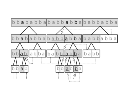
See Figure 1 for an example of a -tree. We can regard the -tree as a binary tree (with the first levels chopped out), where the internal nodes are marked nodes and have two children, whereas the leaves either are marked and represent just one symbol, or are unmarked and represent a pointer to 1 or 2 marked nodes of the same level. If we call the number of leaves, then there are (marked) internal nodes. From the leaves, of them represent single symbols in the last level, while the other leaves are unmarked blocks replaced by pointers. Thus, there are in total nodes in the tree, of which are internal nodes, are pointers, and store explicit symbols. Alternatively, nodes are marked (internal nodes plus leaves) and are unmarked (leaves only).
The -tree then uses space. To obtain a bound in terms of and , note that, at each level, each may mark up to blocks; thus there are marked blocks in total and the -tree uses space.
We now describe two operations on -trees that are fundamental to support efficient indexed searches. The former is also necessary for a self-index, as it allows us extracting arbitrary substrings of efficiently. We remind that this procedure is not the same described on the original structure of string attractors [35], because the structures are also different.
2.1 Extraction
To extract a single symbol , we first map it to a local offset in its corresponding level- block. In general, given the local offset of a character in the current block at level , we first see if the current block is marked. If so, we map to a position in the next level , where the current block is split into two blocks of half the length: if , then we continue on the left child with the same offset; otherwise, we subtract from and continue on the right child. If, instead, is not in a marked block, we take the pointer stored for that block and add to . If the result is , then we continue in the node with offset ; otherwise, we continue in with the offset . In both cases, the new node is marked, so we proceed as on marked blocks in order to move to the next level in constant time. The total time to extract a symbol is then .
2.2 Fingerprinting
We now show that the -tree can be augmented to compute the Karp–Rabin fingerprint of any text substring in logarithmic time.
Lemma 1.
Let have an attractor of size and a Karp–Rabin fingerprint function. Then we can store a data structure of size words supporting the computation of on any substring of in time.
Proof.
We augment our -tree of as follows. At level , we store the Karp–Rabin fingerprints of all the text prefixes ending at positions , for . At levels , we store the fingerprints of all explicit blocks.
We first show that we can reduce the problem to that of computing the fingerprints of two prefixes of explicit blocks. Then, we show how to solve the sub-problem of computing fingerprints of prefixes of explicit blocks.
Let be the substring of which we wish to compute the fingerprint . Note that can be computed in constant time from and so we can assume, without loss of generality, that (i.e., the substring is a prefix of ). Then, at level 0 the substring spans a sequence of blocks followed by a prefix of block (the sequence of blocks or could be empty). The fingerprint of is explicitly stored, so the problem reduces to that of computing the fingerprint of .
We now show how to compute the fingerprint of a prefix of an explicit block (at any level) in time. We distinguish two cases.
(A) We wish to compute the fingerprint of , for some , and is a marked block at level . Let and be the children of at level . Then, the problem reduces to either (i) computing the fingerprint of if , or combining the fingerprints of (which is stored) and . In both sub-cases, the problem reduces to that of computing the fingerprint of the prefix of a block at level , which is explicit since is marked.
(B) We wish to compute the fingerprint of , for some , but is an unmarked explicit block. Then, is linked (through a -tree pointer) to an occurrence in the same level spanning at most two blocks, both of which are marked. If the occurrence of spans only one marked block at level , then and we are back in case (A). Otherwise, the occurrence of spans two marked blocks and at level : , with . For each pointer of this kind in the -tree, we store the fingerprint of . We consider two sub-cases. (B.1) If , then . Since we store the fingerprint of , the problem reduces again to that of computing the fingerprint of the prefix of a marked (explicit) block. (B.2) If , then . Although this is not a prefix nor a suffix of a block, note that . It follows that we can retrieve the fingerprint of in constant time using the fingerprints of and . The latter value is explicitly stored. The former is the fingerprint of the suffix of an explicit (marked) block. In this case, note that the fingerprint of a block’s suffix can be retrieved from the fingerprint of the block and the fingerprint of a block’s prefix, so we are back to the problem of computing the fingerprint of an explicit block’s prefix.
To sum up, computing a prefix of an explicit block at level reduces to the problem of computing a prefix of an explicit block at level (plus a constant number of arithmetic operations to combine values). In the worst case, we navigate down to the leaves, where fingerprints of single characters can be computed in constant time. Combining this procedure into our main algorithm, we obtain the claimed running time of . ∎
3 A Universal Self-Index
Our self-index structure builds on the -tree of . It is formed by two main components: the first finds all the pattern occurrences that cross explicit block boundaries, whereas the second finds the occurrences that are completely inside unmarked blocks.
Lemma 2.
Any substring of length at least either overlaps two consecutive explicit blocks or is completely inside an unmarked block.
Proof.
The leaves of the -tree partition into a sequence of explicit blocks: of those are attractor positions and the other are unmarked blocks. Clearly, if is not completely inside an unmarked block, it must cross a boundary between two explicit blocks. ∎
We exploit the lemma in the following way. We will define an occurrence of as primary if it overlaps two consecutive explicit blocks. The occurrences that are completely contained in an unmarked block are secondary. By the lemma, every occurrence of is either primary or secondary. We will use a data structure to find the primary occurrences and another one to detect the secondary ones. The primary occurrences are found by exploiting the fact that a prefix of matches at the end of an explicit block and the remaining suffix of matches the text that follows. Secondary occurrences, instead, are found by detecting primary or other secondary occurrences within the area where an unmarked block points.
We note that this idea is a variant of the classical one [32] used in all indexes based on LZ77 and CFGs. Now we show that the principle can indeed be applied on attractors, which is the general concept underlying all those compression methods (and others where no indexes exist yet), and therefore unifies all those particular techniques.
3.1 Primary Occurrences
We describe the data structures and algorithms used to find the primary occurrences. Overall, they require space and find the primary occurrences in time , for any constant .
Data Structures.
The leaves of the -tree partition into explicit blocks. The partition is given by the starting positions of the leaves. By Lemma 2, every primary occurrence contains some substring for .
If we find the occurrences considering only their leftmost covered position of the form , we also ensure that each primary occurrence is found once. Thus, we will find primary occurrences as a prefix of appearing at the end of some followed by the corresponding suffix of appearing at the beginning of . For this sake, we define the set of pairs , where means read backwards, and form multisets and with the left and right components of , respectively.
We then lexicographically sort and , to obtain the strings and . All the occurrences ending with a certain prefix of will form a contiguous range in the sorted multiset , whereas all those starting with a certain suffix of will form a contiguous range in the sorted multiset . Each primary occurrence of will then correspond to a pair where both and belong to their range.
Our structure to find the primary occurrences is a two-dimensional discrete grid storing one point for each pair . The grid is of size . We represent using a two-dimensional range search data structure requiring space [12] that reports the points lying inside any rectangle of the grid in time , for any constant . We also store an array that, for each point in , where , stores , that is, where starts in .
Queries.
To search for a pattern , we first find its primary occurrences using as follows. For each partition and , for , we search for and for . For each identified range , we extract all the corresponding primary occurrences in time with our range search data structure. Then we report a primary occurrence starting at for each such point . Over the intervals, this adds up to .
We obtain the ranges in the multiset in overall time , by using the fingerprint-based technique of Gagie et al. [24] applied to the z-fast trie of Belazzougui et al. [2] (we use a lemma from Gagie et al. [26] where the overall result is stated in cleaner form). We use an analogous structure to obtain the ranges in of the suffixes of the reversed pattern.
Lemma 3 (adapted from [26, Lem. 5.2]).
Let be a string on alphabet , be a sorted set of suffixes of , and a Karp–Rabin fingerprint function. If one can extract a substring of length from in time and compute on it in time , then one can build a data structure of size that obtains the lexicographic ranges in of the suffixes of a given pattern in worst-case time — provided that is collision-free among substrings of whose lengths are powers of two.
In Sections 2.1 and 2.2 we show how to extract in time and how to compute a fingerprint in time , respectively. In Section 4.2 we show that a Karp–Rabin function that is collision-free among substrings whose lengths are powers of two can be efficiently found. Together, these results show that we can find all the ranges in and in time .
Patterns of length can be handled as , where stands for any character. Thus, we take and carry out the search as a normal pattern of length . To make this work also for the last position in , we assume as usual that is terminated by a special symbol $ that cannot appear in search patterns . Alternatively, we can store a list of the marked leaves where each alphabet symbol appears, and take those as the primary occurrences. A simple variant of Lemma 2 shows that occurrences of length 1 are either attractor positions or are inside an unmarked block, so the normal mechanism to find secondary occurrences from this set works correctly. Since there are in total such leaves, the space for these lists is .
3.2 Secondary Occurrences
We now describe the data structures and algorithms to find the secondary occurrences. They require space and find the secondary occurrences in time .
Data structures.
To track the secondary occurrences, let us call target and source the text areas and , respectively, of an unmarked block and its pointer, so that there is some contained in (if the blocks are at level , then and ). Let be an occurrence we have already found (using the grid , initially). Our aim is to find all the sources that contain , since their corresponding targets then contain other occurrences of .
To this aim, we store the sources of all levels in an array , with fields and , ordered by starting positions . We build a predecessor search structure on the fields , and a range maximum query (RMQ) data structure on the fields , able to find the maximum endpoint in any given range of . While a predecessor search using space requires time on an -bit-word machine [45, Sec. 1.3.2], the RMQ structure operates in constant time using just bits [21].
Queries.
Let be a primary occurrence found. A predecessor search for gives us the rightmost position where the sources start at . An RMQ on then finds the position of the source with the rightmost endpoint in . If even , then no source covers the occurrence and we finish. If, instead, , then the source covers the occurrence and we process its corresponding target as a secondary occurrence; in this case we also recurse on the ranges and that are nonempty. It is easy to see that each valid secondary occurrence is identified in time (see Muthukrishnan [41] for an analogous process). In addition, such secondary occurrences, , must be recursively processed for further secondary occurrences. A similar procedure is described for tracking the secondary occurrences in the LZ77-index [38].
The cost per secondary occurrence reported then amortizes to a predecessor search, time. This cost is also paid for each primary occurrence, which might not yield any secondary occurrence to amortize it. We now prove that this process is sufficient to find all the secondary occurrences.
Lemma 4.
The described algorithm reports every secondary occurrence exactly once.
Proof.
We use induction on the level of the unmarked block that contains the secondary occurrence. All the secondary occurrences of the last level are correctly reported once, since there are none. Now consider an occurrence inside an unmarked block of level . This block is the target of a source that spans 1 or 2 consecutive marked blocks of level . Then there is another occurrence , with . Note that the algorithm can report only as a copy of . If is primary, then will be reported right after , because , and the algorithm will map to to discover . Otherwise, is secondary, and thus it is within one of the marked blocks at level that overlap the source. Moreover, it is within one of the blocks of level into which those marked blocks are split. Thus, is within an unmarked block of level , which by the inductive hypothesis will be reported exactly once. When is reported, the algorithm will also note that and will find once as well.
If we handle patterns of length by taking the corresponding attractor positions as the primary occurrences, then there may be secondary occurrences in the last level, but those point directly to primary occurrences (i.e., attractor positions), and therefore the base case of the induction holds too. ∎
The total search cost with primary and secondary occurrences is therefore , for any constant defined at indexing time (the choice of affects the constant that accompanies the size of the structure ).
4 Construction
If we allow the index construction to be correct with high probability only, then we can build it in time and space (plus read-only access to ), using a Monte Carlo method. Since is the number of leaves in the -tree and , the time can be written as . In order to ensure a correct index, a Las Vegas method requires time in expectation (and w.h.p.) and space.
4.1 Building the -tree
Given the attractor , we can build the index data structure as follows. At each level , we create an Aho–Corasick automaton [1] on the unmarked blocks at this level (i.e., those at distance from any attractor), and use it to scan the areas around all the attractor elements in order to find a proper pointer for each of those unmarked blocks. This takes time per level. Since the areas around each of the attractor positions are scanned at each level but they have exponentially decreasing lengths, the scanning time adds up to .
As for preprocessing time, each unmarked block is preprocessed only once, and they add up to symbols. The preprocessing can thus be done in time [19]. To be able to scan in linear time, we can build deterministic dictionaries on the edges outgoing from each node, in time [46].
In total, we can build the -tree in deterministic time and space.
To reduce the space to , instead of inserting the unmarked blocks into an Aho–Corasick automaton, we compute their Karp–Rabin fingerprints, store them in a hash table, and scan the areas around attractor elements . This finds the correct sources for all the unmarked blocks w.h.p. Indeed, if we verify the potential collisions, the result is always correct within expected time (further, this time holds w.h.p.).
4.2 Building the Fingerprints
Building the structures for Lemma 1 requires (i) computing the fingerprint of every text prefix ending at block boundaries ( time and space in addition to ), (ii) computing the fingerprint of every explicit block ( time and space starting from the leaves and combining results up to the root), (iii) for each unmarked explicit block , computing the fingerprint of a string of length at most (i.e., the fingerprint of ; see case (B) of Lemma 1). Since unmarked blocks do not have children, each text character is seen at most once while computing these fingerprints, which implies that these values can also be computed in time and space in addition to .
This process, however, does not include finding a collision-free Karp–Rabin hash function. As a result, the fingerprinting is correct w.h.p. only. We can use the de-randomization procedure of Bille et al. [9], which guarantees to find — in expected time222The time is also w.h.p., not only in expectation. and words of space — a Karp–Rabin hash function that is collision-free among substrings of whose lengths are powers of two. This is sufficient to deterministically check the equality of substrings333If the length of the two substrings is not a power of two, then we compare their prefixes and suffixes whose length is the largest power of two smaller than . in the z-fast trie used in the technique [26, Lem. 5.2] that we use to quickly find ranges of pattern suffixes/prefixes (in our Section 3.1).
4.3 Building the Multisets and
To build the multisets and for the primary occurrences, we can build the suffix arrays [40] of and its reverse, . This requires deterministic time and space [31]. Then we can scan those suffix arrays to enumerate and in the lexicographic order.
To sort and within space, we can build instead a sparse suffix tree on the positions of or in . This can be done in expected time (and w.h.p.) and space [27]. If we aim to build the suffix array correctly w.h.p. only, then the time drops to .
We must then build the z-fast trie [2, Thm. 5] on the sets and . Since we can use any space in , we opt for a simpler variant described by Kempa and Kosolobov [34, Lem. 5], which is easier to build. Theirs is a compact trie that stores, for each node representing the string and with parent node : (i) the length , (ii) a dictionary mapping each character to the child node of such that (if such a child exists), and (iii) the (non-extended) fingerprint of , where is the two-fattest number in the range , that is, the number in that range whose binary representation has the largest number of trailing zeros. The trie also requires a global “navigating” hash table that maps the pairs to their corresponding node .
If prefixes some string in (resp. ) and the fingerprint function is collision-free among equal-length text substrings, then their so-called fat binary search procedure finds — in time — the highest node such that is prefixed by a search pattern (assuming constant-time computation of the fingerprint of any substring of , which can be achieved after a linear-time preprocessing of the pattern). The range of strings of (resp. ) is then associated with the node .
Their search procedure, however, has an anomaly [34, Lem. 5]: in some cases it might return a child of instead of . We can fix this problem (and always return the correct ) by also storing, for every internal trie node , the fingerprint of and the exit character . Then, we know that the procedure returned if and only if , the fingerprint of matches that of and . If these conditions do not hold, we know that the procedure returned a child of and we fix the answer by moving to the parent of the returned node.444This fix works in general. In their particular procedure, we do not need to check that (nor to store the exit character). Alternatively, we could directly fix their procedure by similarly storing the fingerprint of (, in their article) and changing line 6 of their extended version [34] to “if nil then ;”.
If does not prefix any string in (resp. ), or if is not collision-free, the search (with our without our fix) returns an arbitrary range. We recall that, to cope with the first condition (which gives the z-fast trie search the name weak prefix search), Lemma 3 adds a deterministic check that allows discarding the incorrect ranges returned by the procedure. The second condition, on the other hand, w.h.p. does not fail. Still, we recall that we can ensure that our function is collision-free by checking, at construction time, for collisions among substrings whose lengths are powers of two, as described in Section 4.2.
The construction of this z-fast trie starts from the sparse suffix tree of (or ), since the topology is the same. The dictionaries giving constant-time access to the nodes’ children can be built correctly w.h.p. in time , or be made perfect in expected time (and w.h.p.) [51]. Alternatively, one can use deterministic dictionaries, which can be built in worst-case time [46]. In all cases, the construction space is . Similarly, the navigating hash can be built correctly w.h.p. in time , or be made perfect in expected time (and w.h.p.) . We could also represent the navigating hash using deterministic dictionaries built in worst-case time [46] and space . The fingerprints and the hashes of the pairs can be computed in total time by using Lemma 1 to compute the Karp–Rabin fingerprints.
4.4 Structures to Track Occurrences
5 Conclusions
We have introduced the first universal self-index for repetitive text collections. The index is based on a recent result [35] that unifies a large number of dictionary compression methods into the single concept of string attractor. For each compression method based on Lempel–Ziv, grammars, run-compressed BWT, collage systems, macro schemes, etc., it is easy to identify an attractor set of the same asymptotic size obtained by the compression method, say . Thus, our construction automatically yields a self-index for each of those compression methods, within space. No structure is known of size able to efficiently extract a substring from the compressed text (say, within time per symbol), and thus is the minimum space we could hope for an efficient self-index with the current state of the art.
Indeed, no self-index of size is known: the smallest ones use [38] and [26] space, respectively, yet there are text families where [25] (where and denote the smallest macro scheme and attractor sizes, respectively). The most time-efficient self-indexes use and space, which is asymptotically equal or larger than ours. The search time of our index, for any constant , is close to that of the fastest of those self-indexes, which were developed for a specific compression format (see [26, Table 1]). Moreover, our construction provides a self-index for compression methods for which no such structure existed before, such as collage systems and macro schemes. Those can provide smaller attractor sets than the ones derived from the more popular compression methods.
We can improve the search time of our index by using slightly more space. Our current bottleneck in the per-occurrence query time is the grid data structure , which uses space and returns each occurrence in time . Instead, a grid structure [12] using space obtains the primary occurrences in time . This slightly larger version of our index can then search in time . This complexity is close to that of some larger indexes in the literature for repetitive string collections (see [26, Table 1]).
A number of avenues for future work are open, including supporting more complex pattern matching, handling dynamic collections of texts, supporting document retrieval, and implementing a practical version of the index. Any advance in this direction will then translate into all of the existing indexes for repetitive text collections.
Acknowledgements
We thank the reviewers for their outstanding job in improving our presentation (and even our bounds).
References
- [1] A. V. Aho and M. J. Corasick. Efficient string matching: an aid to bibliographic search. Communications of the ACM, 18(6):333–340, 1975.
- [2] D. Belazzougui, P. Boldi, R. Pagh, and S. Vigna. Fast prefix search in little space, with applications. In Proc. 18th Annual European Symposium on Algorithms (ESA), pages 427–438, 2010.
- [3] D. Belazzougui and F. Cunial. Fast label extraction in the CDAWG. In Proc. 24th International Symposium on String Processing and Information Retrieval (SPIRE), LNCS 10508, pages 161–175, 2017.
- [4] D. Belazzougui, F. Cunial, T. Gagie, N. Prezza, and M. Raffinot. Composite repetition-aware data structures. In Proc. 26th Annual Symposium on Combinatorial Pattern Matching (CPM), LNCS 9133, pages 26–39, 2015.
- [5] D. Belazzougui, T. Gagie, P. Gawrychowski, J. Kärkkäinen, A. Ordóñez, S. J. Puglisi, and Y. Tabei. Queries on LZ-bounded encodings. In Proc. 25th Data Compression Conference (DCC), pages 83–92, 2015.
- [6] D. Belazzougui and S. J. Puglisi. Range predecessor and Lempel-Ziv parsing. In Proc. 27th Annual ACM-SIAM Symposium on Discrete Algorithms (SODA), pages 2053–2071, 2016.
- [7] D. Belazzougui, S. J. Puglisi, and Y. Tabei. Access, rank, select in grammar-compressed strings. In Proc. 23rd Annual European Symposium on Algorithms (ESA), LNCS 9294, pages 142–154, 2015.
- [8] P. Bille, M. B. Ettienne, I. L. Gørtz, and H. W. Vildhøj. Time-space trade-offs for Lempel-Ziv compressed indexing. Theoretical Computer Science, 713:66–77, 2018.
- [9] P. Bille, I. L. Gørtz, M. B. T. Knudsen, M. Lewenstein, and H. W. Vildhøj. Longest common extensions in sublinear space. In Proc. 26th Annual Symposium on Combinatorial Pattern Matching (CPM), LNCS 9133, pages 65–76, 2015.
- [10] A. Blumer, J. Blumer, D. Haussler, R. McConnell, and A. Ehrenfeucht. Complete inverted files for efficient text retrieval and analysis. Journal of the ACM, 34(3):578–595, 1987.
- [11] M. Burrows and D. Wheeler. A block sorting lossless data compression algorithm. Technical Report 124, Digital Equipment Corporation, 1994.
- [12] T. M. Chan, K. G. Larsen, and M. Pătraşcu. Orthogonal range searching on the RAM, revisited. In Proc. 27th ACM Symposium on Computational Geometry (SoCG), pages 1–10, 2011.
- [13] M. Charikar, E. Lehman, D. Liu, R. Panigrahy, M. Prabhakaran, A. Sahai, and A. Shelat. The smallest grammar problem. IEEE Transactions on Information Theory, 51(7):2554–2576, 2005.
- [14] A. R. Christiansen and M. B. Ettienne. Compressed indexing with signature grammars. In Proc. 13th Latin American Symposium on Theoretical Informatics (LATIN), LNCS 10807, pages 331–345, 2018.
- [15] F. Claude, A. Fariña, M. Martínez-Prieto, and G. Navarro. Universal indexes for highly repetitive document collections. Information Systems, 61:1–23, 2016.
- [16] F. Claude and G. Navarro. Self-indexed grammar-based compression. Fundamenta Informaticae, 111(3):313–337, 2010.
- [17] F. Claude and G. Navarro. Improved grammar-based compressed indexes. In Proc. 19th International Symposium on String Processing and Information Retrieval (SPIRE), LNCS 7608, pages 180–192, 2012.
- [18] M. Crochemore and R. Vérin. Direct construction of compact directed acyclic word graphs. In Proc. 8th Annual Symposium on Combinatorial Pattern Matching (CPM), LNCS 1264, pages 116–129. Springer, 1997.
- [19] S. Dori and G. M. Landau. Construction of Aho Corasick automaton in linear time for integer alphabets. Information Processing Letters, 98(2):66–72, 2006.
- [20] P. Ferragina and G. Manzini. Indexing compressed texts. Journal of the ACM, 52(4):552–581, 2005.
- [21] J. Fischer and V. Heun. Space-efficient preprocessing schemes for range minimum queries on static arrays. SIAM Journal on Computing, 40(2):465–492, 2011.
- [22] T. Gagie. Large alphabets and incompressibility. Information Processing Letters, 99(6):246–251, 2006.
- [23] T. Gagie, P. Gawrychowski, J. Kärkkäinen, Y. Nekrich, and S. J. Puglisi. A faster grammar-based self-index. In Proc. 6th International Conference on Language and Automata Theory and Applications (LATA), LNCS 7183, pages 240–251, 2012.
- [24] T. Gagie, P. Gawrychowski, J. Kärkkäinen, Y. Nekrich, and S. J. Puglisi. LZ77-based self-indexing with faster pattern matching. In Proc. 11th Latin American Symposium on Theoretical Informatics (LATIN), LNCS 8392, pages 731–742, 2014.
- [25] T. Gagie, G. Navarro, and N. Prezza. On the approximation ratio of Lempel-Ziv parsing. In Proc. 13th Latin American Symposium on Theoretical Informatics (LATIN), LNCS 10807, pages 490–503, 2018.
- [26] T. Gagie, G. Navarro, and N. Prezza. Optimal-time text indexing in BWT-runs bounded space. In Proc. 29th Annual ACM-SIAM Symposium on Discrete Algorithms (SODA), pages 1459–1477, 2018.
- [27] P. Gawrychowski and T. Kociumaka. Sparse suffix tree construction in optimal time and space. In Proc. 28th Annual ACM-SIAM Symposium on Discrete Algorithms (SODA), pages 425–439, 2017.
- [28] Y. Han. Deterministic sorting in time and linear space. Journal of Algorithms, 50(1):96–105, 2004.
- [29] A. Jeż. Approximation of grammar-based compression via recompression. Theoretical Computer Science, 592:115–134, 2015.
- [30] A. Jeż. A really simple approximation of smallest grammar. Theoretical Computer Science, 616:141–150, 2016.
- [31] J. Kärkkäinen, P. Sanders, and S. Burkhardt. Linear work suffix array construction. Journal of the ACM, 53(6):918–936, 2006.
- [32] J. Kärkkäinen and E. Ukkonen. Lempel-Ziv parsing and sublinear-size index structures for string matching. In Proc. 3rd South American Workshop on String Processing (WSP), pages 141–155, 1996.
- [33] R. M. Karp and M. O. Rabin. Efficient randomized pattern-matching algorithms. IBM Journal of Research and Development, 31(2):249–260, 1987.
- [34] D. Kempa and D. Kosolobov. LZ-End parsing in compressed space. In Proc. 27th Data Compression Conference (DCC), pages 350–359, 2017. Extended version in https://arxiv.org/pdf/1611.01769.pdf.
- [35] D. Kempa and N. Prezza. At the roots of dictionary compression: String attractors. In Proc. 50th Annual ACM SIGACT Symposium on Theory of Computing (STOC), pages 827–840, 2018.
- [36] T. Kida, T. Matsumoto, Y. Shibata, M. Takeda, A. Shinohara, and S. Arikawa. Collage system: A unifying framework for compressed pattern matching. Theoretical Computer Science, 298(1):253–272, 2003.
- [37] J. C. Kieffer and E. Yang. Grammar-based codes: A new class of universal lossless source codes. IEEE Transactions on Information Theory, 46(3):737–754, 2000.
- [38] S. Kreft and G. Navarro. On compressing and indexing repetitive sequences. Theoretical Computer Science, 483:115–133, 2013.
- [39] A. Lempel and J. Ziv. On the complexity of finite sequences. IEEE Transactions on Information Theory, 22(1):75–81, 1976.
- [40] U. Manber and G. Myers. Suffix arrays: a new method for on-line string searches. SIAM Journal on Computing, 22(5):935–948, 1993.
- [41] S. Muthukrishnan. Efficient algorithms for document retrieval problems. In Proc. 13th Annual ACM-SIAM Symposium on Discrete Algorithms (SODA), pages 657–666, 2002.
- [42] G. Navarro. A self-index on Block Trees. In Proc. 24th International Symposium on String Processing and Information Retrieval (SPIRE), LNCS 10508, pages 278–289, 2017.
- [43] T. Nishimoto, T. I, S. Inenaga, H. Bannai, and M. Takeda. Dynamic index and LZ factorization in compressed space. In Proc. Prague Stringology Conference (PSC), pages 158–170, 2016.
- [44] T. Nishimoto, T. I, S. Inenaga, H. Bannai, and M. Takeda. Fully dynamic data structure for LCE queries in compressed space. In Proc. 41st International Symposium on Mathematical Foundations of Computer Science (MFCS), pages 72:1–72:15, 2016.
- [45] M. Pătraşcu and M. Thorup. Time-space trade-offs for predecessor search. In Proc. 38th Annual ACM Symposium on Theory of Computing (STOC), pages 232–240, 2006.
- [46] M. Ružić. Constructing efficient dictionaries in close to sorting time. In Proc. 35th International Colloquium on Automata, Languages and Programming (ICALP), pages 84–95, 2008.
- [47] W. Rytter. Application of Lempel-Ziv factorization to the approximation of grammar-based compression. Theoretical Computer Science, 302(1-3):211–222, 2003.
- [48] H. Sakamoto. A fully linear-time approximation algorithm for grammar-based compression. Journal of Discrete Algorithms, 3(2–4):416–430, 2005.
- [49] J. A. Storer and T. G. Szymanski. Data compression via textual substitution. Journal of the ACM, 29(4):928–951, 1982.
- [50] P. Weiner. Linear pattern matching algorithms. In Proc. 14th Annual Symposium on Switching and Automata Theory, pages 1–11, 1973.
- [51] D. E. Willard. Examining computational geometry, van Emde Boas trees, and hashing from the perspective of the fusion tree. SIAM Journal on Computing, 29(3):1030–1049, 2000.