Efficient space virtualisation for Hoshen–Kopelman algorithm

Abstract

In this paper the efficient space virtualisation for the Hoshen–Kopelman algorithm is presented. We observe minimal parallel overhead during computations, due to negligible communication costs. The proposed algorithm is applied for computation of random-site percolation thresholds for four dimensional simple cubic lattice with sites’ neighbourhoods containing next-next-nearest neighbours (3NN). The obtained percolation thresholds are $p_{C}(\text{NN})=0.19680(23)$, $p_{C}(\text{2NN})=0.08410(23)$, $p_{C}(\text{3NN})=0.04540(23)$, $p_{C}(\text{2NN+NN})=0.06180(23)$, $p_{C}(\text{3NN+NN})=0.04000(23)$, $p_{C}(\text{3NN+2NN})=0.03310(23)$, $p_{C}(\text{3NN+2NN+NN})=0.03190(23)$, where 2NN and NN stand for next-nearest neighbours and nearest neighbours, respectively.

I Introduction

Percolating systems Broadbent and Hammersley (1957); *Frisch1961; *Frisch1962; Stauffer and Aharony (1994); Bollobás and Riordan (2006); Kesten (1982); Sahimi (1994) are examples of system where purely geometrical phase transition may be observed (see Ref. Saberi (2015) for recent review). The majority of percolating systems which may be mapped to real-world problems deal with two- or three-dimensional space and ranges from condensed matter physics Clancy et al. (2014); *Silva2011; *Shearing2010; *Halperin2010 via rheology Mun et al. (2014); *Amiaz2011; *Bolandtaba2011; *Mourzenko2011 and forest fires Abades et al. (2014); *Camelo-Neto2011; *Guisoni2011; *Simeoni2011; *Kaczanowska2002 to immunology Silverberg et al. (2014); *Suzuki2011; *Lindquist2011; *Naumova2008; *Floyd2008 and quantum mechanics Chandrashekar (2014). However, computer simulations are conducted also for systems with non-physical dimensions $d$ (up to $d=13$) Stauffer and Ziff (2000); Paul et al. (2001); Grassberger (2003); Ballesteros et al. (1997); van der Marck (1998a); van der Marck (1998b).

In classical approach only the nearest neighbours (NN) of sites in $d$-dimensional system are considered. However, complex neighbourhoods may have both, theoretical Balankin et al. (2018); Khatun et al. (2017) and practical Gratens et al. (2007); Bianconi (2013); Masin et al. (2013); Lang et al. (2016); Perets et al. (2017); Haji-Akbari et al. (2015) applications. These complex neighbourhoods may include not only NN but also next-nearest neighbours (2NN) and next-next-nearest neighbours (3NN).

One of the most crucial feature describing percolating systems is a percolation threshold $p_{C}$. In principle, this value separates two phases in the system;

• if sites are occupied with probability $p<p_{C}$ the system behaves as ‘an insulator’,

• while for $p>p_{C}$ the system exhibit attributes of ‘a conductor’.

Namely, for $p=p_{C}$ the giant component containing most of occupied sites appear for the first time. The cluster of occupied sites spans from the one edge of the system to the other one (both being ($d-1$)-dimensional hyper-planes). This allows for direct flow of material (or current) from one to the other edge of the systems. For $p>p_{C}$ this flow is even easier while for $p<p_{C}$ the gaps of unoccupied (empty) sites successfully prevent such flow .

Among so far investigated systems also four dimensional systems were considered Ballesteros et al. (1997); van der Marck (1998a); van der Marck (1998b); Paul et al. (2001); Grassberger (2003). The examples of percolation thresholds for four dimensional lattices and NN neighbours are presented in Tab. 1.

Table 1: The critical values of $p_{C}$ for various four dimensional lattices with NN neighbours and various site coordination number $z$.

lattice	$z$	$p_{C}$	Ref.
diamond	5	0.2978(2)	van der Marck (1998a)
SC	8	0.196901(5)	Ballesteros et al. (1997)
SC	8	0.196889(3)	Paul et al. (2001)
SC	8	0.1968861(14)	Grassberger (2003)
Kagomé	8	0.2715(3)	van der Marck (1998b)
BCC	16	0.1037(3)	van der Marck (1998a)
FCC	24	0.0842(3)	van der Marck (1998a)

In this paper we

• propose an efficient space virtualisation for Hoshen–Kopelman algorithm Hoshen and Kopelman (1976) employed for occupied sites clusters labelling,

• estimate the percolation thresholds for a four dimensional simple cubic (SC) lattice with complex neighbourhoods, i.e. neighbourhoods containing various combinations of NN, 2NN and 3NN neighbours.

While the Hoshen–Kopelman method is good for many problems— for instance, the parallel version of the Hoshen–Kopelman algorithm has been successfully applied for lattice-Boltzmann simulations Frijters et al. (2015)—probably it is not the best method available to find the thresholds. One can even grow single clusters by a Leath type of algorithm Leath (1976), and find the threshold where the size distribution is power-law, as has been done in many works in three dimensions. For high-dimensional percolation, both Grassberger Grassberger (2003), and Mertens and Moore Mertens and Moore (2018) use a method where you do not even have a lattice, but make a list of the coordinates of all the sites that have been visited, and using computer-science type of structures (linked lists and trees, etc.) one can search if a site has already been visited in a short amount of time. Mertens and Moore Mertens and Moore (2017) have also recently proposed an intriguing method where they use basically invasion percolation (along with the various lists) to grow large clusters that self-organize to the critical point. Both groups have gone up to 13 dimensions using these methods.

II Methodology

To evaluate the percolation thresholds the finite-size scaling technique Fisher (1971); Privman (1990); Binder (1992); Landau and Binder (2005) has been applied. According to this theory the quantity $X(p)$ characterising the system in the vicinity of critical point $p_{C}$ scales with the system linear size $L$ as

$$X(p;L)=L^{-x}\cdot\mathcal{F}\left((p-p_{C})L^{1/\nu}\right),$$ (1)

where $\mathcal{F}(\cdot)$ is a scaling function, $x$ is a scaling exponent and $\nu$ is a critical exponent associated with the correlation length Stauffer and Aharony (1994).

For $p=p_{C}$ the value of $L^{x}X(p;L)=\mathcal{F}(0)$ does not depend on the system linear size $L$ which allows for predicting the position of percolation threshold $p_{C}$ as curves $L^{x}X(p;L)$ plotted for various values of $L$ cross each other at $p=p_{C}$. Moreover, for appropriate selection also the value of critical exponent $\nu$ the dependencies $L^{x}X(p;L)$ vs. $\left((p-p_{C})L^{1/\nu}\right)$ collapse into a single curve independently on $L$.

Such technique encounters however one serious problem. Namely, numerically deduced curves $L^{x}X(p;L)$ for various $L$ rather seldom cross each other in a single point, particularly when the number of independent simulations is not huge (see Fig. 1, where examples of dependencies $L^{x}X(p;L)$ for $L=20$, 40, 80 and $R=10^{2}$ (symbols) and $R=10^{4}$ (lines) are presented).

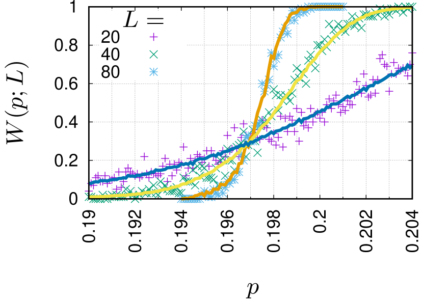
(a) NN

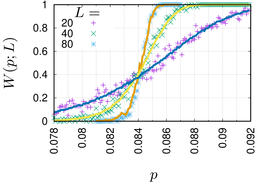
(b) 2NN

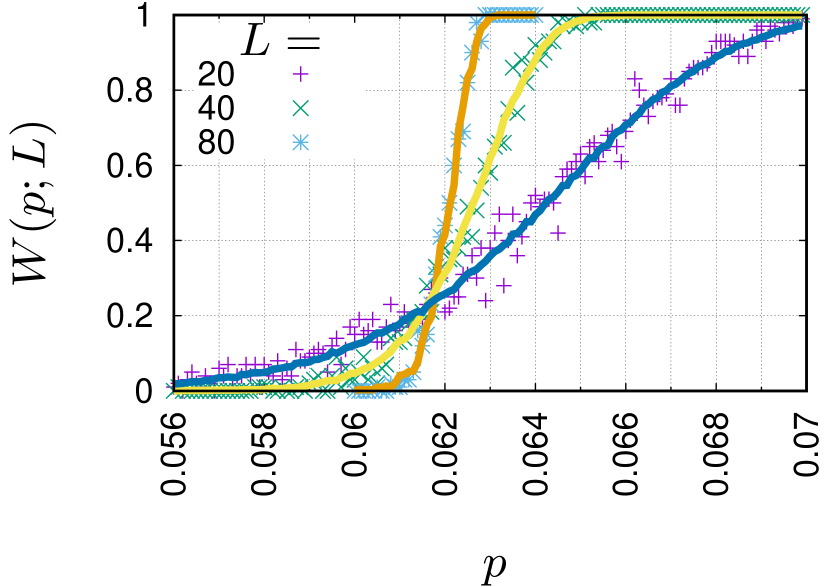
(c) 2NN+NN

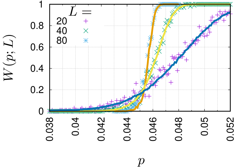
(d) 3NN

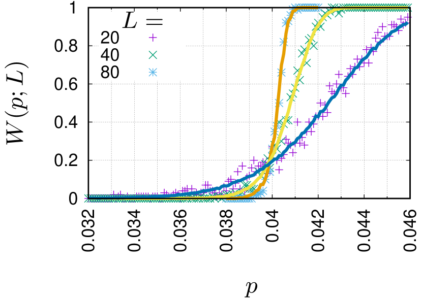
(e) 3NN+NN

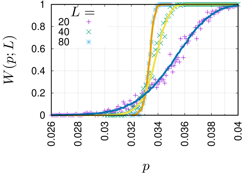
(f) 3NN+2NN

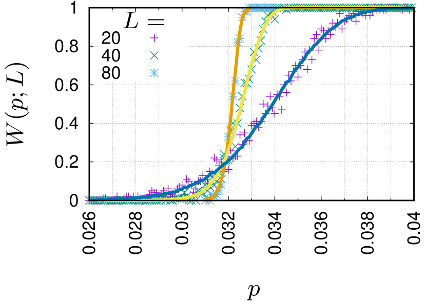
(g) 3NN+2NN+NN

Figure 1: (Colour online). Wrapping probability $W(p;L)$ vs. occupation probability $p$. The results are averaged over $R=10^{2}$ (symbols) or $R=10^{4}$ (lines) simulations.

The remedy for this troubles has been proposed by Bastas et al. Bastas et al. (2011, 2014) and even simplified in Ref. Malarz (2015). The methodology proposed in Ref. Malarz (2015) allows for estimation of percolation threshold $p_{C}$ also for relatively low sampling if the quantity $X(p;L)$ is chosen smartly. Namely, as $X(p;L)$ should be chosen quantity for which scaling exponent $x$ is equal to zero. One of such quantity is the wrapping probability

$$W(p;L)=N(p;L)/R$$ (2)

describing fraction of percolating lattices among $R$ lattices constructed for $pL^{d}$ occupied sites and fixed values of $p$ and $L$, where $d$ is a geometrical space dimension and $N(p;L)$ is a number of percolating lattices.

According to Refs. Bastas et al. (2011, 2014); Malarz (2015) instead of searching common crossing point of $L^{x}X(p;L)$ curves for various $L$ one may wish to minimise

$$\lambda(p)\equiv\sum_{i\neq j}\left[H(p;L_{i})-H(p;L_{j})\right]^{2},$$ (3)

where

$$H(p;L)\equiv W(p;L)+1/W(p;L).$$ (4)

The minimum of $\lambda(p)$ near ‘crossing points’ of $W(p;L)$ curves plotted for various sizes $L$ yields the estimation of percolation threshold $p_{C}$.

Such strategy allowed for estimation of percolation thresholds $p_{C}$ for simple cubic lattice ($d=3$) with complex neighbourhoods (i.e. containing up to next-next-next-nearest neighbours) with relatively low-sampling ($R=10^{4}$) Malarz (2015). Unfortunately, reaching similar accuracy as in Ref. Malarz (2015) for similar linear sizes of the system and for increased space dimension ($d=4$) requires increasing sampling by one order of magnitude (to $R=10^{5}$). This however makes the computations times extremely long. In order to overcome this trouble we propose efficient way of problem parallelisation.

III Computations

Several numerical techniques allow for clusters of connected sites identification Hoshen and Kopelman (1976); Leath (1976); Newman and Ziff (2001); Torin (2014). Here we apply the Hoshen–Kopelman algorithm Hoshen and Kopelman (1976), which allows for sites labelling in a such way, that occupied sites in the same cluster have assigned the same labels and different clusters have different labels associated with them.

The simulations were carried out on Prometheus pro , an Academic Computer Centre Cyfronet AGH-UST operated parallel supercomputer, based on Hewlett–Packard Apollo 8000 Gen9 technology. It consists of 5200 computing 2232 nodes, each with dual 12-core Xeon E5-2680v3 CPUs, interconnected by Infiniband FDR network and over 270 TB of storage space. It supports a wide range of parallel computing tools and applications, including MVAPICH2 MVA MPI implementation for C and Fortran compilers and provides 2.4 PFlops of computing performance, giving it 77th position on November 2017 edition of Supercomputer Top500 list TOP (2017).

III.1 Implementation

One of the problems encountered is high memory size complexity of $\mathcal{O}(L^{4})$, resulting from space being a hyper-cube growing in each direction. The memory limit on the machines the program was run did not allow $L\gg 120$. Several solutions were put in consideration, one of which was splitting single simulations’ calculations between nodes. In the classical version of the algorithm there are sequential dependencies both subsequent 3-$d$ slices perpendicular to the axis of percolation and across any given such slice (see Fig. 2(a)).

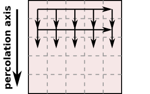
(a) in-domain

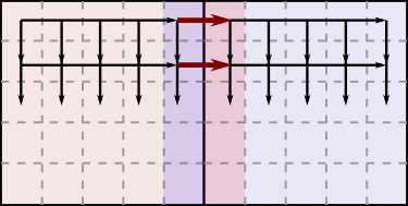
(b) inter-domain

Figure 2: (Colour online). Parallel subdomains 2-$d$ dependencies model: in-domain across slice (thin horizontal arrows), in-domain between slices (thin vertical arrows), inter-domain (bold horizontal arrows).

If speed is to be ignored, sequential dependencies could be simply distributed across the domains. Then a domain succeeding another one in any direction (e.g. blue one succeeding red one on Fig. 2(b)) should be sent information on the class of sites in the area of touch ($L^{3}$ in size) as well as synchronise aliasing arrays. It could be done slice-wise or domain-wise. Slice-wise approach minimises aliasing desynchronisation while domain-wise concentrates communication.

Work between domains can be parallelised. If any domain finds a percolating cluster, it also percolates in the whole hyper-cube, if not, synchronisation of aliasing and both first and last slice cluster ID lists. It requires either totally rebuilding label array or costly label identity checks.

Because of the aforementioned costs and complications, another approach was chosen. Parallelization was only used to accelerate calculations (see Sec. IV.1) while the lack of memory problem was solved using space virtualisation.

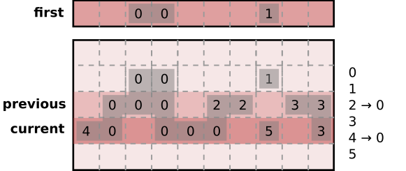
(a) Clustering over adjacent slices

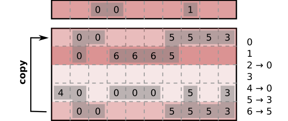
(b) Virtualisation step

Figure 3: (Colour online). Hyperspace buffering in virtualisation (2-$d$ model). Total cost: $\mathcal{O}(L^{4})$, like without buffering.

III.1.1 Message Passing Interface

Message Passing Interface (MPI) Gropp et al. (2014a); *AdvancedMPI2014 is prevailing model of parallel computation on distributed memory systems, including dedicated massively parallel processing supercomputers and cluster systems. It is constructed as a library interface, to be integrated with computer programs written in Fortran or C languages. The main advantage of MPI is its portability and ease of use. Software vendors are presented with clearly defined set of routines that can be implement efficiently, with hardware support provided for specific computer architectures. Several well-tested open-source implementations are also available MPI . The development of MPI specification is maintained by MPI Forum MPI (2017), an academia and industry-based consortium, led by University of Tennessee, Knoxville, TN, USA.

III.1.2 Space virtualisation

Space virtualisation is possible due to the fact there are very limited information that need to be extracted from the hyper-cube, namely: does it contain at least one percolating cluster. However, any percolating cluster is also percolating for a 4-$d$ slice of any depth perpendicular to the percolation axis, including any cut of depth two. Indeed, clusterising any 3-$d$ slice across the percolation axis requires its immediately preceding slice to be fully available as well as clusterised (see Fig. 2(a)). It implies only three slices are essentially needed for calculations: the current one, the previous one and the first one, represented on Fig. 3(a)).

Any iteration over slice buffer introduces additional cost of copying the last slice as the next slice’s immediate predecessor. Due to that, minimal buffer of depth three is highly sub-optimal. For any buffer depth $D$, the additional cost of a single iteration over buffer is $\mathcal{O}(L^{3})$ and $\left\lfloor{L/D}\right\rfloor$ such iterations are needed, for the total cost of buffering being $\mathcal{O}({L^{4}}/{D})$, which implies $D$ should be as big as possible.

In fact, buffering can even benefit performance in some cases as smaller chunk of memory may be possible to fit in cache along with label aliasing array. If so, the cost of copying can be more than compensated by massive reduction of number of memory accesses.

III.1.3 Parallelism

Because calculations are performed sequentially along the percolation axis, sequentially both over a slice and between slices, no asymptotic speed up is gain from that. However, for each state occupation probability $p$, many simulations ($R$) are run for the results to be meaningful, which leads to the total cost of $\mathcal{O}(L^{4}R)$.

As the simulations are fully independent and only their results are to be combined, the program can be speed-up by utilising parallelism over tasks. The only communication needed is collecting the results (whenever a percolating cluster was found or not) at the end of calculations, which is close to $\mathcal{O}(1)$. Theoretical cost is then $\mathcal{O}\left({L^{4}R}/{N}\right)$, where $N$ is the number of computational nodes.

In practice it is unnecessary to map each task to a separate native process, which would require huge amounts of CPU cores (thousands to hundreds of thousands). However, each simulation has a similar execution time, which means no run-time work re-balancing is needed so MPI processes can be used with tasks distributed equally among them. Optimally, the number of processes should be a divisor of $N$.

Utilising more than one process per node puts additional limit on memory, which implies reduction of virtualisation buffer depth. For $N$ nodes and $C$-core architecture that is:

$$D_{2}=D_{1}/C.$$ (5)

This operation implies additional cost of roughly multiplying buffering costs $C$ times, while reducing all costs $C$ times due to multiplying the total number of tasks, which is a clear advantage. Because of that, every core is assigned a separate process.

Threading could be used within a single node but due to close to no communication between tasks, it would make the code more sophisticated with very little performance advantage (only reducing $\mathcal{O}(1)$ cost of communication).

IV Results

IV.1 Speed-up and efficiency

One of the most frequently used performance metric of parallel processing is speedup Wu (1999); Scott et al. (2005). Let $\tau(L^{d},1)$ be the execution time of the sequential algorithm and let $\tau(L^{d},\mathcal{N})$ be the execution of the parallel algorithm executed on $\mathcal{N}$ processors, where $L^{d}$ is the size of the computational problem. A speed-up of parallel computation is defined as

$$\mathcal{S}(\mathcal{N})=\frac{\tau(L^{d},1)}{\tau(L^{d},\mathcal{N})}$$ (6)

the ratio of the sequential execution time to the parallel execution time. One would like to achieve $S(\mathcal{N})=\mathcal{N}$, so called perfect speed-up Amdahl (1967). In this case the problem size stays fixed but the number of processing elements are increased. This are referred to as strong scaling Scott et al. (2005). In general, it is harder to achieve good strong-scaling at larger process counts since the communication overhead for many/most algorithms increases in proportion to the number of processes used.

Another metric to measure the performance of a parallel algorithm is efficiency, $\mathcal{E}$, defined as

$$\mathcal{E}(\mathcal{N})=\frac{\mathcal{S}(\mathcal{N})}{\mathcal{N}}.$$ (7)

Speedup and efficiency are therefore equivalent measures, differing only by the constant factor $\mathcal{N}$.

Fig. 4 demonstrates minimal parallel overhead observed during computations, due to negligible communication costs (see Sec. III.1.3).

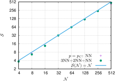
Figure 4: (Colour online). Speed-up $\mathcal{S}$ evaluation for sites labeling at $p=p_{C}$ for NN and 3NN+2NN+NN neighbourhoods and various number of processors $\mathcal{N}$. The values of $\tau(L^{d},1)$ are evaluated for $L=100$ and batch file (Listing 3) parameters ‘-N 1’ (single node) and ‘--ntasks-per-node=1’ (single core), while for $\tau(L^{d},\mathcal{N})$ evaluation we set ‘-N 4’ (and subsequently ‘-N 8’, ‘-N 16’, ‘-N 32’, ‘-N 64’, ‘-N 128’, ‘-N 256’, ‘-N 512’) and again for a signle core (‘--ntasks-per-node=1’). The results are averaged over $R=10^{4}$ simulations.

IV.2 Percolation thresholds

In Fig. 5 we plot wrapping probabilities $W(p;L)$ vs. occupation probability $p$ for various systems sizes $L$ ($40\leq L\leq 140)$ and various complex neighbourhoods (which contain various neighbours from NN to 3NN+2NN+NN). In the same figure we also present the dependencies $\lambda(p)$ in semi-logarithmic scale. The local minimum of $\lambda(p)$ near the interception of $W(p;L)$ for various $L$ indicates the percolation threshold $p_{C}$ obtained with Bastas et al. algorithm.

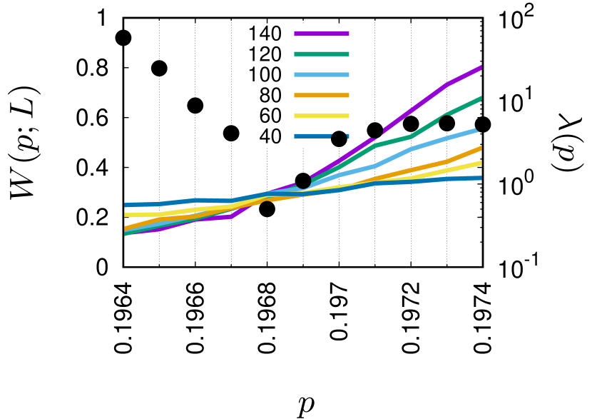
(a) NN

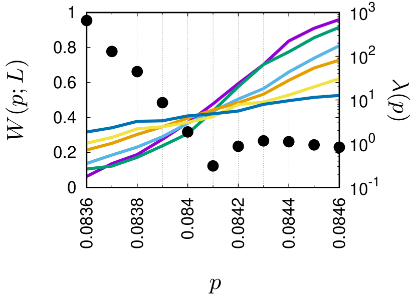
(b) 2NN

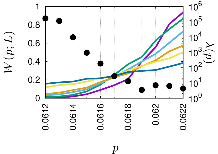
(c) 2NN+NN

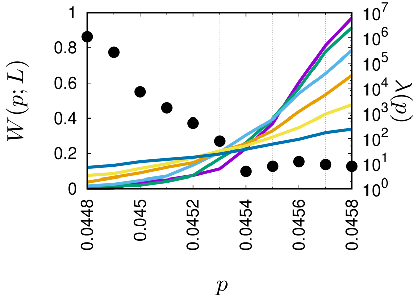
(d) 3NN

(e) 3NN+NN

(f) 3NN+2NN

(g) 3NN+2NN+NN

Figure 5: (Colour online). Wrapping probability $W(p;L)$ (lines, left axis) and the value $\lambda(p)$ (symbols, right axis) vs. occupation probability $p$. The results are averaged over $R=10^{5}$ simulations.

As we can see in Fig. 5 the true value of $p_{C}$ is hidden in the interval of the length of $2\Delta p$, where $\Delta p=10^{-4}$ is the scanning step of occupation probability $p$. With believe that true value of $p_{C}$ is homogeneously distributed in this interval we can estimate the uncertainty of the percolation threshold $u(p_{C})=2\Delta p/\sqrt{3}\approx 0.00023$.

Table 2: The values of percolation thresholds $p_{C}$ for SC lattice in four dimensional space ($d=4$) and for various neighbourhoods as deduced from Fig. 5.

neighbourhood	$z$	$p_{C}$
NN	8	$0.19680(23)$
2NN	24	$0.08410(23)$
2NN+NN	32	$0.06190(23)$
3NN	32	$0.04540(23)$
3NN+NN	40	$0.04000(23)$
3NN+2NN	58	$0.03310(23)$
3NN+2NN+NN	64	$0.03190(23)$

The estimated values of $p_{C}$ together with its uncertainties are collected in Tab. 2. The table shows also the coordination numbers $z$ of sites for every considered complex neighbourhoods ranging from NN to 3NN+2NN+NN.

Please note, that system with 2NN neighbours corresponds to 4-$d$ FCC lattice. The obtained threshold $p_{C}(\text{2NN})\approx 0.08410(23)$ agrees within the error bars with earlier estimation $p_{C}(\text{FCC})\approx 0.0843(3)$ mentioned in Tab. 1.

V Conclusions

In this paper the memory virtualization for the Hoshen–Kopelman Hoshen and Kopelman (1976) is presented. Due to minimal and constant cost of communication between processes the perfect speed-up ($\mathcal{S}(\mathcal{N})\approx\mathcal{N}$) is observed.

The achieved speed-up allows for computation—in reasonable time—the wrapping probabilities $W(p;L)$ (Eq. (2)) up to linear size of $L=140$ in $d=4$ dimensional space, i.e. for systems containg $3.8416\times 10^{8}$ sites realized $10^{4}$ times.

The finite-size scaling technique (see Eq. (1) and Sec. II) combined with Bastas et al. technique Bastas et al. (2011, 2014); Malarz (2015) allows for estimation of percolation thresholds for simple cubic lattice in $d=4$ and for neighbourhoods ranging from NN to 3NN+2NN+NN with the accuracy $u(p_{C})=23\times 10^{-5}$.

The estimated values of $p_{C}$ together with its uncertainties are collected in Tab. 2. Our results enriches earlier studies regarding percolation thresholds for complex neighbourhoods on square Malarz and Galam (2005); *Galam2005b; *Majewski2007 or three-dimensional SC Kurzawski and Malarz (2012); Malarz (2015) lattices.

Appendix A Program description

The program (Listing 1) was written in Fortran 95 Gehrke (1996) and compiled using Intel Fortran compiler ifort. It follows purely procedural paradigm while utilising some array-manipulation features.

The programs parameters are read from command line. All of them are integers and should be simply written one after another, as all of them are mandatory. They are the following:

• L — linear size of the problem,

• p_min — minimal occupation probability to be checked,

• p_max — maximal occupation probability to be checked,

• p_step — loop step over probabilities range,

• N_run — number of simulations for each value of $p$.

All the parameters and dynamically allocated memory is the same through all the program, which loops through over the examined range of probability from p_min to p_max with step p_step. For any given $p$, all processes run subsequent tasks in parallel to each other, only sending results to the main process (through MPI_sum) after finishing all the tasks for the given value of $p$.

Sites are given labels according to Hoshen–Kopelman algorithm. There are two kinds of special labels: FILL_LABEL, having the lowest possible value, and EMPTY_LABEL, having the highest one. Each new casual label is given a successively increasing number. Thanks to that, reclassifying requires no filling checking (although aliasing still does) and checking for percolation is a simple comparison of labels after reclassification: any label with value less than the last label of the first slice is percolating (has_percolation function).

Hyper-cubic space is virtualised (see Sec. III.1) with merged filling and labelling (conditional at l. 173). Then if a new cluster is made (function is_new_cluster), the site is given a label represented by a successive integer number. If not, cluster surrounding the site are merged (subroutine merge_cluster). At the end of the buffer (l. 202-209), the last line is copied before the starting line and the process starts again until the virtual depth of L. The first slice is additionally stored separately (l. 191-199).

The program contains basic time measurement.

Appendix B Source files

The program uses main program (Listing 1), makefile (Listing 2) and batch file (Listing 3).

Makefile is a standard single-target building tool. It provides two commands: ‘build’ (or ‘all’) and ‘clean’. Four parameters can be changed:

• FC — Fortran compiler to be used,

• PAR_FC — Fortran parallel (MPI) compiler to be used,

• RM — cleaning operation,

• SRC — source file.

Batch file runs the executable as a new task on cluster. It contains both program’s run-time parameters and task parameters. Task parameters are the following:

• -J <name> — name of the task,

• -N <number> — number of nodes to run the task on,

• --ntasks-per-node=<number> — number of tasks per node, optimally the same as the number of cores on the given architecture,

• --time=<HH:MM:SS> — time limit for the task,

• -A <grant> — name of the computational grant,

• --output=<file> — file to which the output will be redirected,

• --error=<file> — file to which the error information will be redirected.

Listing 1: Fortan95 code allowing for direct reproduction of the results presented in Figs. 1 and 5.

⬇

1program pi_4d_2n3n4n

2 use ifport, only: rand

3 use mpi

4 implicit none

5

6 ! time measurement

7 real :: start, finish

8

9 ! random seed

10 integer :: seed

11

12 ! loop counters

13 integer :: i_main, i, j, k, m, hb

14 integer :: irun, N_run, maxlabel

15

16 ! maximum L so that the whole hypercube fits into the buffer,

17 ! determines buffer’s size as (MAX_L+4)**4

18 integer, parameter :: MAX_L = 110

19

20 ! minimum depth of the buffer

21 ! the lower, the flatter it can get (and more copying is involved)

22 ! depth is the first dimension (i) so the copying cost should be minimal

23 integer, parameter :: MIN_DEPTH = 10

24

25 ! hypercube’s edge’s length (and length with reserved space)

26 ! experimental limit is L = 418 (L+4 == 422)

27 integer :: L, L4

28

29 ! probability of filling a site

30 real :: p, p_min, p_max, p_step

31

32 ! percentage of systems with a percolating cluster

33 double precision :: perc_local, perc

34

35 ! label for each site

36 integer, dimension(:,:,:,:), allocatable :: label

37

38 ! label reduction (aliasing) table

39 integer, dimension(:), allocatable :: iclass

40

41 ! label for filled sites, has to be smaller than any other label

42 integer :: FILL_LABEL

43

44 ! label for empty sites, has to be greater than any other label

45 integer :: EMPTY_LABEL

46

47 ! communication

48 integer :: world_comm, nproc, rank, root_rank, ierror

49

50 ! string buffer

51 character(len=20) :: str_buffer

52

53 !—————————————————————————

54

55

56 ! start communication

57

58 world_comm = Mpi_Comm_World

59 call Mpi_Init(ierror)

60 call Mpi_Comm_Size(world_comm, nproc, ierror)

61 call Mpi_Comm_Rank(world_comm, rank , ierror)

62 root_rank = 0

63

64 !—————————————————————————

65 ! start random engine

66

67 call system_clock(seed) ! any random seed, basically

68 call srand(seed)

69

70 !—————————————————————————

71 ! read options

72

73 if(rank == root_rank) then

74 call cpu_time(start)

75 end if

76

77 !—————————————————————————

78 ! read parameters

79

80 if(command_argument_count() < 5) then

81 if(rank == root_rank) then

82 print *, ’Too few arguments, expected 5: L, p_min, p_max, p_step, N_run’

83 end if

84 call abort

85 end if

86

87 str_buffer = ""

88 call get_command_argument(1, str_buffer)

89 read(str_buffer, fmt="(I)") L

90 str_buffer = ""

91 call get_command_argument(2, str_buffer)

92 read(str_buffer, fmt="(F)") p_min

93 str_buffer = ""

94 call get_command_argument(3, str_buffer)

95 read(str_buffer, fmt="(F)") p_max

96 str_buffer = ""

97 call get_command_argument(4, str_buffer)

98 read(str_buffer, fmt="(F)") p_step

99 str_buffer = ""

100 call get_command_argument(5, str_buffer)

101 read(str_buffer, fmt="(I)") N_run

102

103 L4 = L**4

104

105 if(rank == root_rank) then

106 print *, ’# 4D: 2N3N4N’

107 print *, ’# L N_run L4’

108 print *, ’#’, L, N_run, L4

109 end if

110

111 !—————————————————————————

112 ! read parameters

113 ! allocate buffer, cluster classes etc.

114

115 associate(depth => space_depth(L+4, L+4, L+4, L+4))

116 if(depth /= L+4) then

117 ! buffering can even give a minor speedup

118 if(depth > MIN_DEPTH) then

119 if(rank == root_rank) then

120 print *, ’# Big L value. Buffering with size: ’, depth

121 end if

122 else

123 if(rank == root_rank) then

124 print *, ’# Too big L value. Abort’

125 end if

126 call abort

127 end if

128 end if

129

130 allocate(label(depth, L+4, L+4, L+4))

131 allocate(iclass(L4/2+2))

132 FILL_LABEL = lbound(iclass, 1)

133 EMPTY_LABEL = ubound(iclass, 1)

134 end associate

135

136 !—————————————————————————

137 ! main calculations part

138

139 ! all processes share the same probability…

140 do p = p_min, p_max, p_step

141

142 perc_local = 0.0d0

143

144 ! …but each process calculates a separate simulation

145 do irun = rank+1, N_run, nproc

146 call initialize(maxlabel, label, iclass)

147

148 ! over the edge with buffer depth as step

149 do i_main = 0, L-1, size(label,1)-4

150 hb = min(ubound(label,1)-2, L-1 - i_main + lbound(label,1)+2)

151

152 do i = lbound(label,1)+2, hb

153 do j = lbound(label,2)+2, ubound(label,2)-2

154 do k = lbound(label,3)+2, ubound(label,3)-2

155 do m = lbound(label,4)+2, ubound(label,4)-2

156 ! labeling clusters

157

158 ! fill randomly + check whether filled or not == just rand

159 if(rand() < p) then

160 if(is_new_cluster(label, i, j, k, m)) then

161 maxlabel = maxlabel+1

162 label(i,j,k,m) = maxlabel

163 else

164 call merge_clusters(label, i, j, k, m, iclass)

165 end if

166 else

167 label(i,j,k,m) = EMPTY_LABEL

168 end if

169 end do

170 end do

171 end do

172 end do

173

174 if(i_main < (L+2) - (size(label,1)-4)) then

175 ! 3D space first in depth

176 ! saved in unused last space as it will be used later

177 if(i_main == 0) then

178 do j = lbound(label,2)+2, ubound(label,2)-2

179 do k = lbound(label,3)+2, ubound(label,3)-2

180 do m = lbound(label,4)+2, ubound(label,4)-2

181 label(ubound(label,1), j, k, m) = label(lbound(label,1)+2, j, k, m)

182 end do

183 end do

184 end do

185 end if

186

187 ! wrapping buffer around

188 do j = lbound(label,2)+2, ubound(label,2)-2

189 do k = lbound(label,3)+2, ubound(label,3)-2

190 do m = lbound(label,4)+2, ubound(label,4)-2

191 label(lbound(label,1)+0, j, k, m) = label(hb-1, j, k, m)

192 label(lbound(label,1)+1, j, k, m) = label(hb-0, j, k, m)

193 end do

194 end do

195 end do

196 end if

197 end do

198

199 ! checking if a cluster is spanning whole system

200

201 ! first 3D space in depth is stored in unused buffer’s part

202 maxlabel = max_source_label(label, ubound(label,1))

203

204 if(has_percolation(label, hb, maxlabel)) then

205 perc_local = perc_local + 1.0d0/(1.0d0*N_run)

206 end if

207 end do

208

209 !—————————————————————————

210 ! get stats from all processes into root process

211

212 call Mpi_Reduce(perc_local, perc, 1, Mpi_Double_Precision, Mpi_Sum, &

213 root_rank, world_comm, ierror)

214

215 ! combine stats

216 if(rank == root_rank) then

217 print ’(F10.6,1X,F7.3)’, p, perc

218 end if

219 end do

220

221 !—————————————————————————

222 ! deallocate buffer, cluster classes etc.

223

224 deallocate(label)

225 deallocate(iclass)

226

227 !—————————————————————————

228 ! show time information

229

230 if(rank == root_rank) then

231 call cpu_time(finish)

232 print ’("# Time = ",f20.3," seconds.")’, finish-start

233 end if

234

235 !—————————————————————————

236 ! finalize communication

237 call Mpi_Finalize(ierror)

238

239

240contains

241 !—————————————————————————

242 ! calculate space depth

243 integer pure function space_depth(N, M, K, L)

244 integer, intent(in) :: N, M, K, L

245

246 space_depth = min((MAX_L+4)**4 / (M*K*L) - 4, N)

247 end function space_depth

248

249 !—————————————————————————

250 ! initialize perlocation to zero

251 subroutine initialize(maxlabel, label, iclass)

252 integer, intent(out) :: maxlabel

253 integer, intent(out), dimension(:,:,:,:) :: label

254 integer, intent(out), dimension(:) :: iclass

255

256 maxlabel = FILL_LABEL + 1

257 label(:,:,:,:) = EMPTY_LABEL

258

259 do i = lbound(iclass, 1), ubound(iclass, 1)

260 iclass(i) = i

261 end do

262 end subroutine

263

264 !—————————————————————————

265 ! whether the given site makes a new cluster

266 logical pure function is_new_cluster(label, i, j, k, m)

267 integer, intent(in), dimension(:,:,:,:) :: label

268 integer, intent(in) :: i, j, k, m

269

270 is_new_cluster = label(i-1,j ,k ,m ) == EMPTY_LABEL .and. &

271 label(i ,j-1,k ,m ) == EMPTY_LABEL .and. &

272 label(i ,j ,k-1,m ) == EMPTY_LABEL .and. &

273 label(i ,j ,k ,m-1) == EMPTY_LABEL .and. &

274

275 label(i-1,j-1,k ,m ) == EMPTY_LABEL .and. &

276 label(i-1,j+1,k ,m ) == EMPTY_LABEL .and. &

277 label(i-1,j ,k-1,m ) == EMPTY_LABEL .and. &

278 label(i-1,j ,k+1,m ) == EMPTY_LABEL .and. &

279 label(i-1,j ,k ,m-1) == EMPTY_LABEL .and. &

280 label(i-1,j ,k ,m+1) == EMPTY_LABEL .and. &

281 label(i ,j-1,k-1,m ) == EMPTY_LABEL .and. &

282 label(i ,j-1,k+1,m ) == EMPTY_LABEL .and. &

283 label(i ,j-1,k ,m-1) == EMPTY_LABEL .and. &

284 label(i ,j-1,k ,m+1) == EMPTY_LABEL .and. &

285 label(i ,j ,k-1,m-1) == EMPTY_LABEL .and. &

286 label(i ,j ,k-1,m+1) == EMPTY_LABEL .and. &

287

288 label(i ,j-1,k-1,m-1) == EMPTY_LABEL .and. &

289 label(i ,j-1,k+1,m-1) == EMPTY_LABEL .and. &

290 label(i ,j-1,k-1,m+1) == EMPTY_LABEL .and. &

291 label(i ,j-1,k+1,m+1) == EMPTY_LABEL .and. &

292 label(i-1,j ,k-1,m-1) == EMPTY_LABEL .and. &

293 label(i-1,j ,k+1,m-1) == EMPTY_LABEL .and. &

294 label(i-1,j ,k-1,m+1) == EMPTY_LABEL .and. &

295 label(i-1,j ,k+1,m+1) == EMPTY_LABEL .and. &

296 label(i-1,j-1,k ,m-1) == EMPTY_LABEL .and. &

297 label(i-1,j+1,k ,m-1) == EMPTY_LABEL .and. &

298 label(i-1,j-1,k ,m+1) == EMPTY_LABEL .and. &

299 label(i-1,j+1,k ,m+1) == EMPTY_LABEL .and. &

300 label(i-1,j-1,k-1,m ) == EMPTY_LABEL .and. &

301 label(i-1,j+1,k-1,m ) == EMPTY_LABEL .and. &

302 label(i-1,j-1,k+1,m ) == EMPTY_LABEL .and. &

303 label(i-1,j+1,k+1,m ) == EMPTY_LABEL

304 end function is_new_cluster

305

306 !—————————————————————————

307 ! merge clusters connecting at the given point

308 subroutine merge_clusters(label, i, j, k, m, iclass)

309 integer, intent(inout), dimension(:,:,:,:) :: label

310 integer, intent(in) :: i, j, k, m

311 integer, intent(inout), dimension(:) :: iclass

312

313 ! reclassifing neighbours

314 ! 2N:

315 call reclassify(label(i-1,j ,k ,m ), iclass)

316 call reclassify(label(i ,j-1,k ,m ), iclass)

317 call reclassify(label(i ,j ,k-1,m ), iclass)

318 call reclassify(label(i ,j ,k ,m-1), iclass)

319

320 ! 3N:

321 call reclassify(label(i-1,j-1,k ,m ), iclass)

322 call reclassify(label(i-1,j+1,k ,m ), iclass)

323 call reclassify(label(i-1,j ,k-1,m ), iclass)

324 call reclassify(label(i-1,j ,k+1,m ), iclass)

325 call reclassify(label(i-1,j ,k ,m-1), iclass)

326 call reclassify(label(i-1,j ,k ,m+1), iclass)

327

328 call reclassify(label(i ,j-1,k-1,m ), iclass)

329 call reclassify(label(i ,j-1,k+1,m ), iclass)

330 call reclassify(label(i ,j-1,k ,m-1), iclass)

331 call reclassify(label(i ,j-1,k ,m+1), iclass)

332

333 call reclassify(label(i ,j ,k-1,m-1), iclass)

334 call reclassify(label(i ,j ,k-1,m+1), iclass)

335

336 ! 4N:

337 call reclassify(label(i-1,j-1,k-1,m ), iclass)

338 call reclassify(label(i-1,j+1,k-1,m ), iclass)

339 call reclassify(label(i-1,j-1,k+1,m ), iclass)

340 call reclassify(label(i-1,j+1,k+1,m ), iclass)

341

342 call reclassify(label(i-1,j ,k-1,m-1), iclass)

343 call reclassify(label(i-1,j ,k+1,m-1), iclass)

344 call reclassify(label(i-1,j ,k-1,m+1), iclass)

345 call reclassify(label(i-1,j ,k+1,m+1), iclass)

346

347 call reclassify(label(i-1,j-1,k ,m-1), iclass)

348 call reclassify(label(i-1,j+1,k ,m-1), iclass)

349 call reclassify(label(i-1,j-1,k ,m+1), iclass)

350 call reclassify(label(i-1,j+1,k ,m+1), iclass)

351

352 call reclassify(label(i ,j-1,k-1,m-1), iclass)

353 call reclassify(label(i ,j-1,k+1,m-1), iclass)

354 call reclassify(label(i ,j-1,k-1,m+1), iclass)

355 call reclassify(label(i ,j-1,k+1,m+1), iclass)

356

357 ! good label according to rule:

358 ! a <= b => iclass(a) <= iclass(b)

359 label(i,j,k,m) = min( &

360 label(i-1,j ,k ,m ), &

361 label(i ,j-1,k ,m ), &

362 label(i ,j ,k-1,m ), &

363 label(i ,j ,k ,m-1), &

364

365 label(i-1,j-1,k ,m ), &

366 label(i-1,j+1,k ,m ), &

367 label(i-1,j ,k-1,m ), &

368 label(i-1,j ,k+1,m ), &

369 label(i-1,j ,k ,m-1), &

370 label(i-1,j ,k ,m+1), &

371 label(i ,j-1,k-1,m ), &

372 label(i ,j-1,k+1,m ), &

373 label(i ,j-1,k ,m-1), &

374 label(i ,j-1,k ,m+1), &

375 label(i ,j ,k-1,m-1), &

376 label(i ,j ,k-1,m+1), &

377

378 label(i ,j-1,k-1,m-1), &

379 label(i ,j-1,k+1,m-1), &

380 label(i ,j-1,k-1,m+1), &

381 label(i ,j-1,k+1,m+1), &

382 label(i-1,j ,k-1,m-1), &

383 label(i-1,j ,k+1,m-1), &

384 label(i-1,j ,k-1,m+1), &

385 label(i-1,j ,k+1,m+1), &

386 label(i-1,j-1,k ,m-1), &

387 label(i-1,j+1,k ,m-1), &

388 label(i-1,j-1,k ,m+1), &

389 label(i-1,j+1,k ,m+1), &

390 label(i-1,j-1,k-1,m ), &

391 label(i-1,j+1,k-1,m ), &

392 label(i-1,j-1,k+1,m ), &

393 label(i-1,j+1,k+1,m ))

394

395 ! make the label common as iclass

396 call make_alias(label, i-1,j,k,m, i,j,k,m)

397 call make_alias(label, i,j-1,k,m, i,j,k,m)

398 call make_alias(label, i,j,k-1,m, i,j,k,m)

399 call make_alias(label, i,j,k,m-1, i,j,k,m)

400

401 call make_alias(label, i-1,j-1,k ,m , i,j,k,m)

402 call make_alias(label, i-1,j+1,k ,m , i,j,k,m)

403 call make_alias(label, i-1,j ,k-1,m , i,j,k,m)

404 call make_alias(label, i-1,j ,k+1,m , i,j,k,m)

405 call make_alias(label, i-1,j ,k ,m-1, i,j,k,m)

406 call make_alias(label, i-1,j ,k ,m+1, i,j,k,m)

407 call make_alias(label, i ,j-1,k-1,m , i,j,k,m)

408 call make_alias(label, i ,j-1,k+1,m , i,j,k,m)

409 call make_alias(label, i ,j-1,k ,m-1, i,j,k,m)

410 call make_alias(label, i ,j-1,k ,m+1, i,j,k,m)

411 call make_alias(label, i ,j ,k-1,m-1, i,j,k,m)

412 call make_alias(label, i ,j ,k-1,m+1, i,j,k,m)

413

414 call make_alias(label, i ,j-1,k-1,m-1, i,j,k,m)

415 call make_alias(label, i ,j-1,k+1,m-1, i,j,k,m)

416 call make_alias(label, i ,j-1,k-1,m+1, i,j,k,m)

417 call make_alias(label, i ,j-1,k+1,m+1, i,j,k,m)

418 call make_alias(label, i-1,j ,k-1,m-1, i,j,k,m)

419 call make_alias(label, i-1,j ,k+1,m-1, i,j,k,m)

420 call make_alias(label, i-1,j ,k-1,m+1, i,j,k,m)

421 call make_alias(label, i-1,j ,k+1,m+1, i,j,k,m)

422 call make_alias(label, i-1,j-1,k ,m-1, i,j,k,m)

423 call make_alias(label, i-1,j+1,k ,m-1, i,j,k,m)

424 call make_alias(label, i-1,j-1,k ,m+1, i,j,k,m)

425 call make_alias(label, i-1,j+1,k ,m+1, i,j,k,m)

426 call make_alias(label, i-1,j-1,k-1,m , i,j,k,m)

427 call make_alias(label, i-1,j+1,k-1,m , i,j,k,m)

428 call make_alias(label, i-1,j-1,k+1,m , i,j,k,m)

429 call make_alias(label, i-1,j+1,k+1,m , i,j,k,m)

430 end subroutine merge_clusters

431

432 !—————————————————————————

433 ! get maximal label for the 3D space first in depth

434 integer pure function max_source_label(label, row)

435 integer, intent(in), dimension(:,:,:,:) :: label

436 integer, intent(in) :: row

437 integer :: j, k, m

438

439 max_source_label = 0

440 do j = lbound(label,2)+2, ubound(label,2)-2

441 do k = lbound(label,3)+2, ubound(label,3)-2

442 do m = lbound(label,4)+2, ubound(label,4)-2

443 if(label(row, j, k, m) /= EMPTY_LABEL) then

444 max_source_label = max(max_source_label, &

445 label(row, j, k, m))

446 end if

447 end do

448 end do

449 end do

450 end function max_source_label

451

452 !—————————————————————————

453 ! whether there is a percolation or not

454 logical pure function has_percolation(label, row, maxlabel)

455 integer, intent(in), dimension(:,:,:,:) :: label

456 integer, intent(in) :: row, maxlabel

457 integer :: j, k, m

458

459 has_percolation = .false.

460 do j = lbound(label,2)+2, ubound(label,2)-2

461 do k = lbound(label,3)+2, ubound(label,3)-2

462 do m = lbound(label,4)+2, ubound(label,4)-2

463 if(label(row, j, k, m) <= maxlabel) then

464 has_percolation = .true.

465 return

466 end if

467 end do

468 end do

469 end do

470 end function has_percolation

471

472 !—————————————————————————

473 ! reduce site’s label’s aliasing

474 ! (assign it its non-aliasing label)

475 subroutine reclassify(ix, iclass)

476 integer, intent(inout) :: ix

477 integer, intent(in), dimension(:) :: iclass

478

479 do while (iclass(ix) /= ix)

480 ix = iclass(ix)

481 end do

482 end subroutine reclassify

483

484 !—————————————————————————

485 ! makes one site’s cluster an alias for another one

486 subroutine make_alias(label, i1, j1, k1, m1, i2, j2, k2, m2)

487 integer, dimension(:,:,:,:), intent(inout) :: label

488 integer, intent(in) :: i1,j1,k1,m1, i2,j2,k2,m2

489

490 if(label(i1,j1,k1,m1) /= EMPTY_LABEL) then

491 iclass(label(i1,j1,k1,m1)) = label(i2,j2,k2,m2)

492 end if

493 end subroutine

494

495

496end program pi_4d_2n3n4n

Listing 2: Makefile

⬇

1RM=rm

2FC=ifort

3PAR_FC=mpiifort

4

5FLAGS = -g -O3 -no-prec-div -fp-model fast=2 -xHost -ipo -warn all

6

7SRC=pi_4d_2n3n4n.f90

8OBJ=${SRC:.f90=.o}

9EXE=${SRC:.f90=.exe}

10

11

12.PHONY: all

13all: build

14

15.PHONY: build

16build: $(EXE)

17

18

19$(EXE): $(OBJ)

20 $(PAR_FC) $(FLAGS) -o $@ $< -module .

21

22$(OBJ): $(SRC)

23 $(PAR_FC) $(FLAGS) -c -o $@ $<

24

25

26.PHONY: clean

27clean:

28 $(RM) -f $(EXE) *.o *.mod

Listing 3: Batch file

⬇

1#!/bin/bash -l

2#SBATCH -J L80_2N3N4N

3#SBATCH -N 100

4#SBATCH –ntasks-per-node=24

5#SBATCH –time=1:00:00

6#SBATCH -A hk4d3nn

7#SBATCH –output="pi_4d_2n3n4n.out"

8#SBATCH –error="pi_4d_2n3n4n.err"

9

10cd $SLURM_SUBMIT_DIR

11

12module add plgrid/tools/impi

13export FORT_BUFFERED=yes

14

15mpiexec -env I_MPI_FABRICS shm:dapl -env I_MPI_FABRICS_LIST dapl -env I_MPI_DAPL_UD=enable -env MPIEXEC_PREFIX_DEFAULT=out ./pi_4d_2n3n4n.exe 80 0.030 0.034 0.0001 10000

References

- Broadbent and Hammersley (1957) S. R. Broadbent and J. M. Hammersley, “Percolation processes,” Mathematical Proceedings of the Cambridge Philosophical Society 53, 629–641 (1957).
- Frisch et al. (1961) H. L. Frisch, E. Sonnenblick, V. A. Vyssotsky, and J. M. Hammersley, “Critical percolation probabilities (site problem),” Physical Review 124, 1021–1022 (1961).
- Frisch et al. (1962) H. L. Frisch, J. M. Hammersley, and D. J. A. Welsh, “Monte Carlo estimates of percolation probabilities for various lattices,” Physical Review 126, 949–951 (1962).
- Stauffer and Aharony (1994) D. Stauffer and A. Aharony, Introduction to Percolation Theory, 2nd ed. (Taylor and Francis, London, 1994).
- Bollobás and Riordan (2006) B. Bollobás and O. Riordan, Percolation (Cambridge UP, Cambridge, 2006).
- Kesten (1982) H. Kesten, Percolation Theory for Mathematicians (Brikhauser, Boston, 1982).
- Sahimi (1994) M. Sahimi, Applications of Percolation Theory (Taylor and Francis, London, 1994).
- Saberi (2015) A. A. Saberi, “Recent advances in percolation theory and its applications,” Physics Reports 578, 1–32 (2015).
- Clancy et al. (2014) J. P. Clancy, A. Lupascu, H. Gretarsson, Z. Islam, Y. F. Hu, D. Casa, C. S. Nelson, S. C. LaMarra, G. Cao, and Young-June Kim, “Dilute magnetism and spin-orbital percolation effects in ,” Physical Review B 89, 054409 (2014).
- Silva et al. (2011) J. Silva, R. Simoes, S. Lanceros-Mendez, and R. Vaia, “Applying complex network theory to the understanding of high-aspect-ratio carbon-filled composites,” EPL 93, 37005 (2011).
- Shearing et al. (2010) P. R. Shearing, D. J. L. Brett, and N. P. Brandon, “Towards intelligent engineering of sofc electrodes: a review of advanced microstructural characterisation techniques,” International Material Reviews 55, 347–363 (2010).
- Halperin and Bergman (2010) B. I. Halperin and D. J. Bergman, “Heterogeneity and disorder: Contributions of Rolf Landauer,” Physica B 405, 2908–2914 (2010).
- Mun et al. (2014) S. C. Mun, M. Kim, K. Prakashan, H. J. Jung, Y. Son, and O O. Park, “A new approach to determine rheological percolation of carbon nanotubes in microstructured polymer matrices,” Carbon 67, 64–71 (2014).
- Amiaz et al. (2011) Y. Amiaz, S. Sorek, Y. Enzel, and O. Dahan, “Solute transport in the vadose zone and groundwater during flash floods,” Water Resources Research 47, W10513 (2011).
- Bolandtaba and Skauge (2011) S. F. Bolandtaba and A. Skauge, “Network modeling of EOR processes: A combined invasion percolation and dynamic model for mobilization of trapped oil,” Transport in Porous Media 89, 357–382 (2011).
- Mourzenko et al. (2011) V. V. Mourzenko, J. F. Thovert, and P. M. Adler, “Permeability of isotropic and anisotropic fracture networks, from the percolation threshold to very large densities,” Physical Review E 84, 036307 (2011).
- Abades et al. (2014) S. R. Abades, A. Gaxiola, and P. A. Marquet, “Fire, percolation thresholds and the savanna forest transition: a neutral model approach,” Journal of Ecology 102, 1386–1393 (2014).
- Camelo-Neto and Coutinho (2011) G. Camelo-Neto and S. Coutinho, “Forest-fire model with resistant trees,” Journal of Statistical Mechanics—Theory and Experiment 2011, P06018 (2011).
- Guisoni et al. (2011) N. Guisoni, E. S. Loscar, and E. V. Albano, “Phase diagram and critical behavior of a forest-fire model in a gradient of immunity,” Physical Review E 83, 011125 (2011).
- Simeoni et al. (2011) A. Simeoni, P. Salinesi, and F. Morandini, “Physical modelling of forest fire spreading through heterogeneous fuel beds,” International Journal of Wildland Fire 20, 625–632 (2011).
- Malarz et al. (2002) K. Malarz, S. Kaczanowska, and K. Kułakowski, “Are forest fires predictable?” International Journal of Modern Physics C 13, 1017–1031 (2002).
- Silverberg et al. (2014) J. L. Silverberg, A. R. Barrett, M. Das, P. B. Petersen, L. J. Bonassar, and I. Cohen, “Structure-function relations and rigidity percolation in the shear properties of articular cartilage,” Biophysical Journal 107, 1721–1730 (2014).
- Suzuki and Sasaki (2011) S. U. Suzuki and A. Sasaki, “How does the resistance threshold in spatially explicit epidemic dynamics depend on the basic reproductive ratio and spatial correlation of crop genotypes?” Journal of Theoretical Biology 276, 117–125 (2011).
- Lindquist et al. (2011) J. Lindquist, J. Ma, P. van den Driessche, and F. H. Willeboordse, “Effective degree network disease models,” Journal of Mathematical Biology 62, 143–164 (2011).
- Naumova et al. (2008) E. N. Naumova, J. Gorski, and Yu. N. Naumov, “Simulation studies for a multistage dynamic process of immune memory response to influenza: experiment in silico,” Ann. Zool. Fenn. 45, 369–384 (2008).
- Floyd et al. (2008) W. Floyd, L. Kay, and M. Shapiro, “Some elementary properties of SIR networks or, can I get sick because you got vaccinated?” Bulletin of Mathematical Biology 70, 713–727 (2008).
- Chandrashekar (2014) Th. Chandrashekar, C. M. Busch, “Quantum percolation and transition point of a directed discrete-time quantum walk,” Scientific Reports 4, 6583 (2014).
- Stauffer and Ziff (2000) D. Stauffer and R. M. Ziff, “Reexamination of seven-dimensional site percolation threshold,” International Journal of Modern Physics C 11, 205–209 (2000).
- Paul et al. (2001) G. Paul, R. M. Ziff, and H. E. Stanley, “Percolation threshold, Fisher exponent, and shortest path exponent for four and five dimensions,” Physical Review E 64, 026115 (2001).
- Grassberger (2003) P. Grassberger, “Critical percolation in high dimensions,” Physical Review E 67, 036101 (2003).
- Ballesteros et al. (1997) H. G. Ballesteros, L. A. Fernández, V. Martín-Mayor, A. Muñoz Sudupe, G. Parisi, and J. J. Ruiz-Lorenzo, “Measures of critical exponents in the four-dimensional site percolation,” Physics Letters B 400, 346–351 (1997).
- van der Marck (1998a) S. C. van der Marck, “Calculation of percolation thresholds in high dimensions for fcc, bcc and diamond lattices,” International Journal of Modern Physics C 09, 529–540 (1998a).
- van der Marck (1998b) S. C. van der Marck, “Site percolation and random walks on -dimensional Kagomé lattices,” Journal of Physics A: Mathematical and General 31, 3449 (1998b).
- Balankin et al. (2018) A. S. Balankin, M. A. Martinez-Cruz, O. Susarrey-Huerta, and L. Damian Adame, “Percolation on infinitely ramified fractal networks,” Physics Letters A 382, 12–19 (2018).
- Khatun et al. (2017) T. Khatun, T. Dutta, and S. Tarafdar, “‘Islands in sea’ and ‘lakes in mainland’ phases and related transitions simulated on a square lattice,” European Physical Journal B 90, 213 (2017).
- Gratens et al. (2007) X. Gratens, A. Paduan-Filho, V. Bindilatti, N. F. Oliveira, Jr., and Y. Shapira, “Magnetization-step spectra of (CH3-NH3)2MnxCd1-xCl4 at 20 mK: Fine structure and the second-largest exchange constant,” Physical Review B 75, 184405 (2007).
- Bianconi (2013) G. Bianconi, “Superconductor-insulator transition in a network of 2d percolation clusters,” EPL 101, 26003 (2013).
- Masin et al. (2013) M. Masin, L. Bergqvist, J. Kudrnovsky, M. Kotrla, and V. Drchal, “First-principles study of thermodynamical properties of random magnetic overlayers on fcc-Cu(001) substrate,” Physical Review B 87, 075452 (2013).
- Lang et al. (2016) G. Lang, L. Veyrat, U. Graefe, F. Hammerath, D. Paar, G. Behr, S. Wurmehl, and H. J. Grafe, “Spatial competition of the ground states in 1111 iron pnictides,” Physical Review B 94, 014514 (2016).
- Perets et al. (2017) Yu. Perets, L. Aleksandrovych, M. Melnychenko, O. Lazarenko, L. Vovchenko, and L. Matzui, “The electrical properties of hybrid composites based on multiwall carbon nanotubes with graphite nanoplatelets,” Nanoscale Research Letters 12, 406 (2017).
- Haji-Akbari et al. (2015) A. Haji-Akbari, N. Haji-Akbari, and R. M. Ziff, “Dimer covering and percolation frustration,” Physical Review E 92, 032134 (2015).
- Note (1) The terminology of material flow between edges of the system comes from the original papers introducing the percolation term Broadbent and Hammersley (1957); *Frisch1961; *Frisch1962 in the subject of rheology.
- Hoshen and Kopelman (1976) J. Hoshen and R. Kopelman, “Percolation and cluster distribution. 1. cluster multiple labeling technique and critical concentration algorithm,” Physical Review B 14, 3438–3445 (1976).
- Frijters et al. (2015) S. Frijters, T. Krüger, and J. Harting, “Parallelised Hoshen–Kopelman algorithm for lattice-Boltzmann simulations,” Computer Physics Communications 189, 92–98 (2015).
- Leath (1976) P. L. Leath, “Cluster shape and critical exponents near percolation threshold,” Physical Review Letter 36, 921–924 (1976).
- Mertens and Moore (2018) S. Mertens and C. Moore, “Percolation thresholds and Fisher exponents in hypercubic lattices,” Physical Review E 98, 022120 (2018).
- Mertens and Moore (2017) S. Mertens and C. Moore, “Percolation thresholds in hyperbolic lattices,” Physical Review E 96, 042116 (2017).
- Fisher (1971) M. E. Fisher, “The theory of critical point singularities,” in Critical Phenomena, edited by M. S. Green (Academic Press, London, 1971) pp. 1–99.
- Privman (1990) V. Privman, “Finite-size scaling theory,” in Finite size scaling and numerical simulation of statistical systems, edited by V. Privman (World Scientific, Singapore, 1990) p. 1.
- Binder (1992) K. Binder, “Finite size effects at phase transitions,” in Computational Methods in Field Theory, edited by C. B. Lang and H. Gausterer (Springer, Berlin, 1992) pp. 59–125.
- Landau and Binder (2005) D. P. Landau and K. Binder, A Guide to Monte Carlo Simulations in Statistical Physics, 2nd ed. (Cambridge UP, Cambridge, 2005) pp. 77–90.
- Bastas et al. (2011) N. Bastas, K. Kosmidis, and P. Argyrakis, “Explosive site percolation and finite-size hysteresis,” Physical Review E 84, 066112 (2011).
- Bastas et al. (2014) N. Bastas, K. Kosmidis, P. Giazitzidis, and M. Maragakis, “Method for estimating critical exponents in percolation processes with low sampling,” Physical Review E 90, 062101 (2014).
- Malarz (2015) K. Malarz, “Simple cubic random-site percolation thresholds for neighborhoods containing fourth-nearest neighbors,” Physical Review E 91, 043301 (2015).
- Newman and Ziff (2001) M. E. J. Newman and R. M. Ziff, “Fast Monte Carlo algorithm for site or bond percolation,” Physical Review E 64, 016706 (2001).
- Torin (2014) I. V. Torin, “New algorithm to test percolation conditions within the Newman–Ziff algorithm,” International Journal of Modern Physics C 25, 1450064 (2014).
- (57) “Prometheus,” Accademic Computer Center Cyfronet AGH-UST, Kraków, Poland. Accessed: 2018-03-14.
- (58) “MVAPICH: MPI over InfiniBand, Omni-Path, Ethernet/iWARP, and RoCE,” Network-Based Computing Laboratory, Ohio State University, Columbus, OH. Accessed: 2018-03-14.
- TOP (2017) “The TOP500 list,” (2017), nERSC/Lawrence Berkeley National Laboratory, University of Tennessee, Knoxville, Prometeus GmbH, Sinsheim, Germany. Accessed: 2018-03-14.
- Gropp et al. (2014a) W. Gropp, E. Lusk, and A. Skjellum, Using MPI, 3rd ed. (MIT Press, 2014).
- Gropp et al. (2014b) W. Gropp, T. Hoefler, R. Thakur, and E. Lusk, Using Advanced MPI (MIT Press, 2014).
- (62) “MPICH—A high-performance and widely portable implementation of the Message Passing Interface,” Argonne National Laboratory, Argonne, IL. Accessed: 2018-03-14.
- MPI (2017) “MPI forum—standardization forum for the Message Passing Interface,” (2017), TU München, University of Tennessee, Knoxville, TN, US. Accessed: 2018-03-14.
- Wu (1999) X. Wu, Performance Evaluation, Prediction and Visualization of Parallel Systems (Springer, 1999).
- Scott et al. (2005) L. R. Scott, T. Clark, and B. Bagheri, Scientific Parallel Computing (Princeton University Press, Princeton, NJ, 2005).
- Amdahl (1967) G. M. Amdahl, “Validity of the single processor approach to achieving large scale computing capabilities,” in Proceedings of the April 18-20, 1967, Spring Joint Computer Conference, AFIPS ’67 (Spring) (ACM, New York, NY, USA, 1967) pp. 483–485.
- Malarz and Galam (2005) K. Malarz and S. Galam, “Square-lattice site percolation at increasing ranges of neighbor bonds,” Physical Review E 71, 016125 (2005).
- Galam and Malarz (2005) S. Galam and K. Malarz, “Restoring site percolation on damaged square lattices,” Physical Review E 72, 027103 (2005).
- Majewski and Malarz (2007) M. Majewski and K. Malarz, “Square lattice site percolation thresholds for complex neighbourhoods,” Acta Physica Polonica B 38, 2191–2199 (2007).
- Kurzawski and Malarz (2012) Ł. Kurzawski and K. Malarz, “Simple cubic random-site percolation thresholds for complex neighbourhoods,” Reports on Mathematical Physics 70, 163–169 (2012).
- Gehrke (1996) W. Gehrke, Fortran 95 Language Guide (Springer-Verlag, London, 1996).