A general white noise test based on kernel lag-window estimates of the spectral density operator

Abstract

We propose a general white noise test for functional time series based on estimating a distance between the spectral density operator of a weakly stationary time series and the constant spectral density operator of an uncorrelated time series. The estimator that we propose is based on a kernel lag-window type estimator of the spectral density operator. When the observed time series is a strong white noise in a real separable Hilbert space, we show that the asymptotic distribution of the test statistic is standard normal, and we further show that the test statistic diverges for general serially correlated time series. These results recover as special cases those of Hong (1996) and Horváth et al. (2013). In order to implement the test, we propose and study a number of kernel and bandwidth choices, including a new data adaptive bandwidth, as well as data adaptive power transformations of the test statistic that improve the normal approximation in finite samples. A simulation study demonstrated that the proposed method has good size and improved power when compared to other methods available in the literature, while also offering a light computational burden.

Keywords: time series, functional data, serial correlation, spectral density operator, kernel estimator.

MSC2010: 62M10, 62G10, 62M15.

1 Introduction

With this paper, we aim to contribute to the growing literature on general white noise tests for functional time series. The scope of methodology for analyzing time series taking values in a function space has grown substantially over the last two decades; see Bosq, (2000) for seminal work on linear processes in function space, and Hörmann and Kokoszka, (2012), as well as Chapters 13–16 of Horváth and Kokoszka, (2012) for more recent reviews. Most methods are still founded on non-parametric and non-likelihood based approaches that rely on the estimation of autocovariance operators to quantify serial dependence in the sequence; see, e.g., Kargin and Onatski, (2008); Klepsch and Klüppelberg, (2017); Panaretos and Tavakoli, (2013); Zhang and Shao, (2015). It is then often of interest to measure whether or not an observed sequence of curves, or model residuals, exhibit significant autocorrelation.

Quite a large number of methods have been introduced in order to test for serial correlation in the setting of functional time series. These methods build upon a well developed literature on portmanteau tests for scalar and multivariate time series, see e.g. Li, (2004) and Chapter 5 of Francq and Zakoïan, (2010) for a summary, and can be grouped along the classical time series dichotomy of time domain and spectral domain approaches. In the time domain, Gabrys and Kokoszka, (2007) proposed a method based on applying a multivariate portmanteau test to vectors of scores obtained from projecting the functional time series into a few principal directions. Horváth et al., (2013) and Kokoszka et al., (2017) develop portmanteau tests based directly on the norms of empirical autocovariance operators. In the spectral domain, Zhang, (2016) and Bagchi et al., (2018) develop test statistics based on measuring the difference between periodogram operators and the spectral density operator under the assumption that the sequence is a weak white noise. Among these, the tests of Horváth et al., (2013), Zhang, (2016) and Bagchi et al., (2018) are general white noise tests in the sense that they are asymptotically consistent against serial correlation at any lag, whereas the other tests cited utilize only the autocovariance information up to a user selected maximum lag, and do not have more than trivial power for serial correlation occurring beyond that lag.

Each of these statistics are indelibly connected in that they reduce to weighted sums of semi-norms of empirical autocovariance operators, and hence it is natural to consider alternate ways of choosing the weights in order to increase power; see Escanciano and Lobato, (2009) for a nice discussion of these connections for scalar portmanteau tests. The statistics developed in Zhang, (2016) and Bagchi et al., (2018), which are based on the periodogram operator, effectively give equal weights to the autocovariance operators at all lags. One might expect then that reweighting the periodogram so that it is a more efficient estimate of the spectral density operator might lead to more powerful tests. A sensible and well studied method of choosing these weights is to employ a kernel and lag-window or bandwidth as is common in nonparametric spectral density operator estimation. Panaretos and Tavakoli, (2013) were the first to put forward similar estimators of the spectral density operator based on smoothing the periodogram operator for $L^{2}([0,1],\mathbb{R})$-valued time series. Hong, (1996) developed general white noise tests for scalar sequences based on this principle by comparing kernel lag-window estimates of the spectral density to the constant spectral density of a weak white noise, which were further studied and extended in Shao, 2011b and Shao, 2011a .

In this paper, we develop a general white noise test based on kernel lag-window estimators of the spectral density operator of a time series with values in a separable Hilbert space $\mathbb{H}$. Under standard conditions on the kernel and bandwidth used, we show that the estimated distance between the spectral density operator and the constant spectral density operator based on such estimators can be normalized to have an asymptotic standard normal distribution when the observed series is a strong white noise. We further show that this standardized distance diverges in probability to infinity at a quantifiable rate under general departures from a weak white noise.

These results compare to and generalize the main results of Horváth et al., (2013). Letting $n$ denote the length of the functional time series and $p_{n}$ denote the bandwidth parameter, the main result of Horváth et al., (2013) establishes the asymptotic normality of the unweighted sum of the norms of empirical autocovariance operators up to a bandwidth $p_{n}$ satisfying $p_{n}\to\infty$, $p_{n}=O(\log(n))$, as $n\to\infty$. Our main result establishes this under the less restrictive conditions on the bandwidth $p_{n}\to\infty$, $p_{n}=o(n)$, while also allowing for a general class of weights in the sum. This condition on the bandwidth is optimal in the sense that without it the corresponding kernel lag-window estimator of the spectral density cannot generally be consistent in mean squared norm sense. These improvements owe primarily to a new, more general, method of proof relying on a martingale central limit theorem.

Implementing the test requires the choice of a kernel and bandwidth, and we suggest several methods for this, including a new data driven and kernel adaptive bandwidth. We also investigate power transformations of our test statistics that improve their size properties in finite samples. We investigated these results and various choices of the kernel and bandwidth by means of a Monte Carlo simulation study, which confirm that the proposed tests have good size as well as power exceeding currently available tests, although with the drawback that they are not built for general white noise (e.g. functional conditionally heteroscedastic) series.

The rest of the paper is organized as follows. We present in Section 2 our main methodological contributions and theory, including all asymptotic results for the proposed test statistic and its power transformation. In Section 3, we discuss some details of implementing the proposed test, and present the results of a Monte Carlo simulation study. The practical utility of the proposed tests are illustrated in Section 4 with an application to Eurodollar futures curves. Some concluding remarks are given in Section 5, and all proofs as well as the definition of the data adaptive bandwidth are given in the Appendix following the references.

2 Statement of method and main results

We first define some notation that is used throughout the paper. Suppose that $\mathbb{H}$ is a real separable Hilbert space with the inner product $\langle\cdot,\cdot\rangle:\mathbb{H}\times\mathbb{H}\to\mathbb{R}$. For $x,y\in\mathbb{H}$, the tensor of $x$ and $y$ is a rank one operator $x\otimes y:\mathbb{H}\to\mathbb{H}$ defined by $(x\otimes y)(z)=\langle z,y\rangle x$ for each $z\in\mathbb{H}$. Let $\{u_{t}\}_{t\in\mathbb{Z}}$ be a second-order stationary sequence of $\mathbb{H}$-valued random elements. Throughout we make use of the following moment conditions:

Assumption 1.

$\operatorname{E}u_{t}=0$ and $\operatorname{E}\|u_{t}\|^{4}<\infty$ for each $t\in\mathbb{Z}$.

The autocovariance operators of $\{u_{t}\}_{t\in\mathbb{Z}}$ are defined by

$$\mathcal{C}(j)=\operatorname{E}[u_{j}\otimes u_{0}],\quad j\in\mathbb{Z}.$$ (1)

The spectral density operator $\mathcal{F}(\omega)$ with $\omega\in[-\pi,\pi]$ is the discrete-time Fourier transform of the sequence of autocovariance operators $\{\mathcal{C}(j)\}_{j\in\mathbb{Z}}$ defined by

$$\mathcal{F}(\omega)=(2\pi)^{-1}\sum_{j\in\mathbb{Z}}\mathcal{C}(j)e^{-\mathbf{i}j\omega},\quad\omega\in[-\pi,\pi],$$ (2)

where $\mathbf{i}=\sqrt{-1}$. $\mathcal{F}(\omega)$ is well-defined for $\omega\in[-\pi,\pi]$ provided that $\sum_{j\in\mathbb{Z}}|\kern-1.07639pt|\kern-1.07639pt|\mathcal{C}(j)|\kern-1.07639pt|\kern-1.07639pt|_{2}<\infty$, where $|\kern-1.07639pt|\kern-1.07639pt|\cdot|\kern-1.07639pt|\kern-1.07639pt|_{2}$ is the Hilbert-Schmidt norm. We say that $\{u_{t}\}_{t\in\mathbb{Z}}$ is a weak white noise if $\mathcal{C}(j)=0$ for $j\neq 0$, and evidently in this case $\mathcal{F}(\omega)=(2\pi)^{-1}\mathcal{C}(0)$ is constant as a function of $\omega\in[-\pi,\pi]$.

2.1 Definition of test statistic and null asymptotics

In order to measure the proximity of a given functional time series process $\{u_{t}\}_{t\in\mathbb{Z}}$ to a white noise, it is natural then to consider the distance $Q$, in terms of integrated normed error, between the spectral density operator $\mathcal{F}(\omega)$, $\omega\in[-\pi,\pi]$, and $(2\pi)^{-1}\mathcal{C}(0)$:

$$Q^{2}=2\pi\int_{-\pi}^{\pi}|\kern-1.07639pt|\kern-1.07639pt|\mathcal{F}(\omega)-(2\pi)^{-1}\mathcal{C}(0)|\kern-1.07639pt|\kern-1.07639pt|_{2}^{2}d\omega.$$

$Q$ specifically measures how far the second-order structure of $\{u_{t}\}_{t\in\mathbb{Z}}$ deviates from that of a weak white noise. Given a sample $u_{1},\ldots,u_{n}$ from $\{u_{t}\}_{t\in\mathbb{Z}}$, we are then interested in testing the hypothesis

$$H_{0}:\ Q=0\quad\text{versus}\quad H_{1}:Q>0.$$

Zhang, (2016) and Bagchi et al., (2018) develop general tests of $H_{0}$ versus $H_{1}$. In this paper, we focus on testing $H_{1}$ versus the stronger but still relevant hypothesis

$$H_{0,\text{iid}}:\mbox{the sequence $\{u_{t}\}_{t\in\mathbb{Z}}$ is independent and identically distributed in $\mathbb{H}$}.$$

We discuss in Section 5 how one might adapt the proposed test statistic to generally test $H_{0}$ versus $H_{1}$, but we do not pursue this in detail here. One can estimate $Q$ via estimates of $\mathcal{F}(\omega)$, $\omega\in[-\pi,\pi]$, and $\mathcal{C}(0)$. The sample autocovariance operators are defined by

$$\hat{\mathcal{C}}_{n}(j)=n^{-1}\sum_{t=j+1}^{n}u_{t}\otimes u_{t-j},\quad 0\leq j<n,$$ (3)

and $\hat{\mathcal{C}}_{n}(j)=\hat{\mathcal{C}}_{n}^{*}(-j)$ for $-n<j<0$, where ^∗ denotes the adjoint of an operator. The spectral density operator may be estimated using a kernel lag-window estimator defined by

$$\hat{\mathcal{F}}_{n}(\omega)=(2\pi)^{-1}\sum_{|j|<n}k(j/p_{n})\hat{\mathcal{C}}_{n}(j)e^{-\mathbf{i}j\omega},\quad\omega\in[-\pi,\pi],$$ (4)

where $k:\mathbb{R}\to[-1,1]$ is a kernel and $p_{n}$ is the lag-window or bandwidth parameter. We make the following assumptions on the kernel $k$ and $p_{n}$.

Assumption 2.

$k:\mathbb{R}\to[-1,1]$ is a symmetric function that is continuous at zero and at all but finite number of points, with $k(0)=1$ and $k(x)=O(x^{-\alpha})$, for some $\alpha>1/2$ as $x\to\infty$.

Assumption 3.

$p_{n}$ satisfies that $p_{n}\to\infty$ and $p_{n}/n\to 0$ as $n\to\infty$.

Assumption 2 covers all typically used kernels in the literature on spectral density estimation, and guarantees that integrals of the form $\int_{-\infty}^{\infty}k^{r}(x)dx$ are finite, for $r=2,4$. The above estimates yield an estimate of $Q$ defined by

$$\hat{Q}_{n}^{2}=2\pi\int_{-\pi}^{\pi}|\kern-1.07639pt|\kern-1.07639pt|\hat{\mathcal{F}}_{n}(\omega)-(2\pi)^{-1}\hat{\mathcal{C}}_{n}(0)|\kern-1.07639pt|\kern-1.07639pt|_{2}^{2}d\omega.$$

Using the fact that $|\kern-1.07639pt|\kern-1.07639pt|\cdot|\kern-1.07639pt|\kern-1.07639pt|_{2}^{2}=\langle\cdot,\cdot\rangle_{\mathrm{HS}}$, where $\langle\cdot,\cdot\rangle_{\mathrm{HS}}$ is the Hilbert-Schmidt inner product and the fact that the functions $\{e_{k}\}_{k\in\mathbb{Z}}$ defined by $e_{k}(x)=e^{-{\mathbf{i}}kx}$ for $k\in\mathbb{Z}$ and $x\in[-\pi,\pi]$ are orthonormal in $L^{2}[-\pi,\pi]$, we obtain

$$\hat{Q}_{n}^{2}=\sum_{0<|j|<n}k^{2}(j/p_{n})|\kern-1.07639pt|\kern-1.07639pt|\hat{\mathcal{C}}_{n}(j)|\kern-1.07639pt|\kern-1.07639pt|_{2}^{2}.$$

Further, since the kernel $k$ is symmetric, $\hat{\mathcal{C}}_{n}(-j)=\hat{\mathcal{C}}_{n}^{*}(j)$, and $|\kern-1.07639pt|\kern-1.07639pt|\hat{\mathcal{C}}_{n}^{*}(j)|\kern-1.07639pt|\kern-1.07639pt|_{2}=|\kern-1.07639pt|\kern-1.07639pt|\hat{\mathcal{C}}_{n}(j)|\kern-1.07639pt|\kern-1.07639pt|_{2}$, we also have that

$$\hat{Q}_{n}^{2}=2\sum_{j=1}^{n-1}k^{2}(j/p_{n})|\kern-1.07639pt|\kern-1.07639pt|\hat{\mathcal{C}}_{n}(j)|\kern-1.07639pt|\kern-1.07639pt|_{2}^{2}.$$

Remarkably, $\hat{Q}_{n}^{2}$ can be normalized under these general conditions in order to satisfy the central limit theorem under $H_{0,\text{iid}}$, and we now proceed by defining the normalizing sequences and constants needed to do so. Let $\sigma^{2}=\operatorname{E}\|u_{0}\|^{2}$, $\mu_{4}=\operatorname{E}\|u_{0}\|^{4}$ and $\hat{\sigma}_{n}^{2}=n^{-1}\sum_{t=1}^{n}\|u_{t}\|^{2}$. Also, let us denote

$$C_{n}(k)=\sum_{j=1}^{n-1}(1-j/n)k^{2}(j/p_{n})\quad\text{and}\quad D_{n}(k)=\sum_{j=1}^{n-2}(1-j/n)(1-(j+1)/n)k^{4}(j/p_{n}).$$

We propose to use the test statistic $T_{n}$ defined by

$$T_{n}=T_{n}(k,p_{n})=\frac{2^{-1}n\hat{Q}_{n}^{2}-\hat{\sigma}_{n}^{4}C_{n}(k)}{|\kern-1.07639pt|\kern-1.07639pt|\hat{\mathcal{C}}_{n}(0)|\kern-1.07639pt|\kern-1.07639pt|_{2}^{2}\sqrt{2D_{n}(k)}},\quad n\geq 1.$$ (5)

We now state our main result, which establishes the asymptotic normality of $T_{n}$.

Theorem 1.

Suppose that $\{u_{t}\}_{t\in\mathbb{Z}}$ satisfies $H_{0,\text{iid}}$ and that Assumptions 1, 2, and 3 hold. Then

$$T_{n}\xrightarrow{d}N(0,1)\quad\text{as}\quad n\to\infty.$$ (6)

Remark 1.

Let us observe that

$$T_{n}=\frac{\hat{\sigma}_{n}^{4}}{|\kern-1.07639pt|\kern-1.07639pt|\hat{\mathcal{C}}_{n}(0)|\kern-1.07639pt|\kern-1.07639pt|_{2}^{2}}\cdot\frac{2^{-1}n\hat{\sigma}_{n}^{-4}\hat{Q}_{n}^{2}-C_{n}(k)}{\sqrt{2D_{n}(k)}},\quad n\geq 1.$$ (7)

If $\mathbb{H}=\mathbb{R}$, then it follows that $\hat{\sigma}_{n}^{2}/|\kern-1.07639pt|\kern-1.07639pt|\hat{\mathcal{C}}_{n}(0)|\kern-1.07639pt|\kern-1.07639pt|_{2}\stackrel{{\scriptstyle p}}{{\to}}1$ as $n\to\infty$, and we recover precisely the test statistic proposed by Hong, (1996) (see the statistic $M_{1n}$ on page 840 of Hong, (1996)). In a general real separable Hilbert space $\mathbb{H}$, $\hat{\sigma}_{n}^{2}/|\kern-1.07639pt|\kern-1.07639pt|\hat{\mathcal{C}}_{n}(0)|\kern-1.07639pt|\kern-1.07639pt|_{2}$ converges in probability to $\sigma^{2}/|\kern-1.07639pt|\kern-1.07639pt|\mathcal{C}(0)|\kern-1.07639pt|\kern-1.07639pt|_{2}$, which need not equal one. Intuitively, the structure “inside” $u_{t}$ determines the value of $\sigma^{2}/|\kern-1.07639pt|\kern-1.07639pt|\mathcal{C}(0)|\kern-1.07639pt|\kern-1.07639pt|_{2}$.

Remark 2.

Under Assumptions 2 and 3, we have that $D_{n}(k)=D(k)p_{n}+o(p_{n})$ as $n\to\infty$, where $D(k)=\int_{0}^{\infty}k^{4}(z)dz$.

Remark 3.

Taking the kernel $k$ to be the truncated kernel, $k=\mathds{1}_{\{|x|\leq 1\}}$, one has that

$$\hat{Q}_{n}^{2}=2\sum_{j=1}^{p_{n}}|\kern-1.07639pt|\kern-1.07639pt|\hat{\mathcal{C}}_{n}(j)|\kern-1.07639pt|\kern-1.07639pt|_{2}^{2}.$$

Additionally if $p_{n}/\sqrt{n}\to 0$, then also $C_{n}(k)/p_{n}\to 1$, and $D_{n}(k)/p_{n}\to 1$ as $n\to\infty$. It follows then under these and the conditions of Theorem 1 that the statistic $T_{n}$ is asymptotically equivalent with

$$T_{n}^{*}=\frac{n\sum_{j=1}^{p_{n}}|\kern-1.07639pt|\kern-1.07639pt|\hat{\mathcal{C}}_{n}(j)|\kern-1.07639pt|\kern-1.07639pt|_{2}^{2}-\hat{\sigma}_{n}^{4}p_{n}}{|\kern-1.07639pt|\kern-1.07639pt|\hat{\mathcal{C}}_{n}(0)|\kern-1.07639pt|\kern-1.07639pt|_{2}^{2}\sqrt{2p_{n}}}$$

which is identical to the statistic considered in Horváth et al., (2013). It was shown there that this statistic has a normal limit under $H_{0,\text{iid}}$ and the assumption that $p_{n}\to\infty$, $p_{n}=O(\log(n))$ as $n\to\infty$. Therefore Theorem 1 can be viewed as a generalisation of their result.

2.2 Transformation of test statistic

Chen and Deo, (2004) investigated the finite sample performance of the test statistic of Hong, (1996), and found that the sampling distribution of the test statistic under $H_{0,iid}$ tends to be right skewed, causing the test to be oversized. We confirm their findings in our simulation study in Section 3 as the test statistic $T_{n}$ suffers from the same problem in the general Hilbert space setting as well. In order to alleviate this, Chen and Deo, (2004) suggests a power transformation of the test statistic of the form

$$T_{n}^{\beta}=\frac{(2^{-1}n\hat{\sigma}_{n}^{-4}\hat{Q}_{n}^{2})^{\beta}-[C_{n}^{\beta}(k)+2^{-1}\beta(\beta-1)C_{n}^{\beta-2}(k)\hat{\sigma}_{n}^{-8}|\kern-1.07639pt|\kern-1.07639pt|\hat{\mathcal{C}}_{n}(0)|\kern-1.07639pt|\kern-1.07639pt|_{2}^{4}2D_{n}(k)]}{\beta C_{n}^{\beta-1}(k)\hat{\sigma}_{n}^{-4}|\kern-1.07639pt|\kern-1.07639pt|\hat{\mathcal{C}}_{n}(0)|\kern-1.07639pt|\kern-1.07639pt|_{2}^{2}[2D_{n}(k)]^{1/2}}$$

for $n\geq 1$ with $\beta\neq 0$. It follows from Theorem 1 and the application of the delta method that $T_{n}^{\beta}\xrightarrow{d}N(0,1)$ as $n\to\infty$ for $\beta\neq 0$.

Chen and Deo, (2004) then recommend to choose the value of $\beta$ in order to make approximate skewness of $T_{n}^{\beta}$ equal to zero. In order to describe how to achieve this in our setting, let us suppose that $Z$ is a Gaussian random element with values in $S_{2}(\mathbb{H})$ such that $\operatorname{E}Z=0$ and the covariance operator of $Z$ is given by $\mathcal{A}=\operatorname{E}[u_{0}\otimes u_{1}\tilde{\otimes}u_{0}\otimes u_{1}]$, where $S_{2}(\mathbb{H})$ is the space of the Hilbert-Schmidt operators from $\mathbb{H}$ to $\mathbb{H}$ and $\tilde{\otimes}$ denotes the tensor of two elements of $S_{2}(\mathbb{H})$. As a result of the central limit theorem applied to the estimated covariance operators $\hat{\mathcal{C}}_{n}(j)$, $2^{-1}n\hat{Q}_{n}^{2}$ is approximately a weighted sum of independent and identically distributed random variables with the distribution of $|\kern-1.07639pt|\kern-1.07639pt|Z|\kern-1.07639pt|\kern-1.07639pt|_{2}^{2}$. From this we can obtain the approximate skewness of $(2^{-1}n\hat{Q}_{n}^{2})^{\beta}$ using Taylor’s theorem (see Chen and Deo, (2004) for more details). The value of $\beta$ which makes the approximate skewness equal to zero is given by

$$\beta^{*}=1-\frac{\mu_{1}^{\prime}\mu_{3}}{3\mu_{2}^{2}}\frac{[\sum_{j=1}^{n-1}k^{2}(j/p_{n})][\sum_{j=1}^{n-1}k^{6}(j/p_{n})]}{[\sum_{j=1}^{n-1}k^{4}(j/p_{n})]^{2}},$$ (8)

where $\mu_{1}^{\prime}=\operatorname{E}|\kern-1.07639pt|\kern-1.07639pt|Z|\kern-1.07639pt|\kern-1.07639pt|_{2}^{2}$, $\mu_{2}=\operatorname{Var|\kern-1.07639pt|\kern-1.07639pt|Z|\kern-1.07639pt|\kern-1.07639pt|_{2}^{2}}$ and $\mu_{3}=\operatorname{E}[|\kern-1.07639pt|\kern-1.07639pt|Z|\kern-1.07639pt|\kern-1.07639pt|_{2}^{2}-\operatorname{E}|\kern-1.07639pt|\kern-1.07639pt|Z|\kern-1.07639pt|\kern-1.07639pt|_{2}^{2}]^{3}$.

If $\mathbb{H}=\mathbb{R}$, $|\kern-1.07639pt|\kern-1.07639pt|Z|\kern-1.07639pt|\kern-1.07639pt|_{2}^{2}$ is distributed as a scaled $\chi^{2}(1)$ random variable, and then $\mu_{1}^{\prime}\mu_{3}/(3\mu_{2}^{2})=2/3$. Consequently, $\beta^{*}$ in the univariate case only depends on the sample size $n$, the kernel $k$ and the bandwidth $p_{n}$. The choice of $\mu_{1}^{\prime}\mu_{3}/(3\mu_{2}^{2})=2/3$ even in the general setting can be motivated by using a Welch–Satterthwaite style approximation of the norm of a Gaussian process $|\kern-1.07639pt|\kern-1.07639pt|Z|\kern-1.07639pt|\kern-1.07639pt|_{2}^{2}$ with a scaled chi-squared distribution; see for instance Zhang, (2013) and Krishnamoorthy, (2016). However, in the general Hilbert space setting the value of $\mu_{1}^{\prime}\mu_{3}/(3\mu_{2}^{2})$ depends on the data and should be estimated. Let us suppose that $\{v_{k}\}_{k\geq 1}$ are the eigenvectors of $\mathcal{A}$ with the corresponding eigenvalues $\{\lambda_{k}\}_{k\geq 1}$. We have that

$$|\kern-1.07639pt|\kern-1.07639pt|Z|\kern-1.07639pt|\kern-1.07639pt|_{2}^{2}=\sum_{k\geq 1}|\langle Z,v_{k}\rangle_{\mathrm{HS}}|^{2}=\sum_{k\geq 1}\lambda_{k}|\lambda_{k}^{-1/2}\langle Z,v_{k}\rangle_{\mathrm{HS}}|^{2}=\sum_{k\geq 1}\lambda_{k}\xi_{k},$$

where $\{\xi_{k}\}_{k\geq 1}$ are independent and identically distributed $\chi^{2}(1)$ random variables. It follows by calculating the cumulant generating function of $|\kern-1.07639pt|\kern-1.07639pt|Z|\kern-1.07639pt|\kern-1.07639pt|_{2}^{2}$ that

$$\mu_{1}^{\prime}=\sum_{k\geq 1}\lambda_{k}=\operatorname{Tr}\mathcal{A},\quad\mu_{2}=2\sum_{k\geq 1}\lambda_{k}^{2}=2\operatorname{Tr}\mathcal{A}^{2}\quad\text{and}\quad\mu_{3}=8\sum_{k\geq 1}\lambda_{k}^{3}=8\operatorname{Tr}\mathcal{A}^{3},$$

where $\operatorname{Tr}$ denotes the trace of an operator and $\mathcal{A}^{k}$ denotes the $k$-fold compositon of the operator with itself. By Lemma 5 in Appendix B,

$$\operatorname{Tr}\mathcal{A}=[\operatorname{Tr}\mathcal{C}(0)]^{2},\quad\operatorname{Tr}\mathcal{A}^{2}=[\operatorname{Tr}\mathcal{C}^{2}(0)]^{2}\quad\text{and}\quad\operatorname{Tr}\mathcal{A}^{3}=[\operatorname{Tr}\mathcal{C}^{3}(0)]^{2}$$

and we can estimate $\mu_{1}^{\prime}$, $\mu_{2}$ and $\mu_{3}$ by estimating $\mathcal{C}(0)$ using the estimator $\hat{\mathcal{C}}_{n}(0)$ given by (3). It follows that the plug-in estimators of $\mu_{1}^{\prime}$, $\mu_{2}$ and $\mu_{3}$ are given by

$$\hat{\mu}_{1}^{\prime}=n^{-1}\sum_{t=1}^{n}\|u_{t}\|^{2},\quad\hat{\mu}_{2}=n^{-2}\sum_{s,t=1}^{n}|\langle u_{t},u_{s}\rangle|^{2}$$ (9)

and

$$\hat{\mu}_{3}=n^{-3}\sum_{r,s,t=1}^{n}\langle u_{t},u_{s}\rangle\langle u_{s},u_{r}\rangle\langle u_{r},u_{t}\rangle.$$ (10)

These results motivate two tests of $H_{0,\text{iid}}$ each with asymptotic size $\alpha\in(0,1)$: to Reject $H_{0,\text{iid}}$ if $T_{n}\geq\Phi^{-1}(1-\alpha)$ or $T_{n}^{\beta}\geq\Phi^{-1}(1-\alpha)$ with $\beta\neq 0$, where $\Phi^{-1}(1-\alpha)$ is the $1-\alpha$ quantile of the standard normal distribution. The finite sample properties of each of these tests for various choices of the bandwidth and kernel, as well as a comparison of these tests to existing methods, are presented in Section 3.

2.3 Consistency

We now establish the consistency of our test under $H_{1}$. In order to describe time series $\{u_{t}\}_{t\in\mathbb{Z}}$ that are generally weakly dependent, we follow Tavakoli, (2014) and introduce cumulant summability conditions. Suppose that $\{u_{t}\}_{t\in\mathbb{Z}}$ is a sequence of $\mathbb{H}$-valued random elements. We say that $\{u_{t}\}_{t\in\mathbb{Z}}$ is $k$-th order stationary with $k\geq 1$ if $\operatorname{E}\|u_{t}\|^{k}<\infty$ for all $t\in\mathbb{Z}$ and, for all $t_{1},\ldots,t_{l}\in\mathbb{Z}$ and $l=1,\ldots,k$,

$$\operatorname{E}[u_{t_{1}}\otimes u_{t_{2}}\otimes\ldots\otimes u_{t_{l}}]=\operatorname{E}[u_{0}\otimes u_{t_{2}-t_{1}}\otimes\ldots\otimes u_{t_{l}-t_{1}}].$$

The joint cumulant of real or complex-valued random variables $X_{1},\ldots,X_{k}$ such that $\operatorname{E}|X_{j}|^{k}<\infty$ for all $j=1,\ldots,k$ with $k\geq 1$ is given by

$$\operatorname{cum}(X_{1},\ldots,X_{k})=\sum_{\pi}(|\pi|-1)!(-1)^{|\pi|-1}\prod_{B\in\pi}\operatorname{E}\Bigl{[}\prod_{i\in B}X_{i}\Bigr{]},$$

where $\pi$ runs through the list of all partitions of $\{1,\ldots,n\}$, $B$ runs through the list of all blocks of the partition $\pi$, and $|\pi|$ is the number of parts in the partition; see Brillinger, (2001) for more details. Suppose that $u_{1},\ldots,u_{k}$ are $\mathbb{H}$-valued random variables such that $\operatorname{E}\|u_{j}\|^{k}<\infty$ for all $j=1,\ldots,k$. The $k$-th order cumulant $\operatorname{cum}(u_{1},\ldots,u_{k})$ is a unique element in $\bigotimes_{j=1}^{k}\mathbb{H}$ that satisfies

$$\langle\operatorname{cum}(u_{1},\ldots,u_{k}),f_{1}\otimes\ldots\otimes f_{k}\rangle=\operatorname{cum}(\langle u_{1},f_{1}\rangle,\ldots,\langle u_{k},f_{k}\rangle)$$

for all $f_{1},\ldots,f_{k}\in\mathbb{H}$. Suppose that $\{u_{t}\}_{t\in\mathbb{Z}}$ is $2k$-th order stationary and let us denote

$$\mathcal{K}_{t_{1},\ldots,t_{2k-1}}=\operatorname{cum}(u_{t_{1}},\ldots,u_{t_{2k-1}},u_{t_{0}})$$

for $t_{1},\ldots,t_{2k-1}\in\mathbb{Z}$. Then $\mathcal{K}_{t_{1},\ldots,t_{2k-1}}$ is an operator that maps the elements of $\bigotimes_{j=1}^{k}\mathbb{H}$ to $\bigotimes_{j=1}^{k}\mathbb{H}$ such that

$$\langle\mathcal{K}_{t_{1},\ldots,t_{2k-1}}(f_{k+1}\otimes\ldots\otimes f_{2k}),f_{1}\otimes\ldots\otimes f_{k}\rangle\\ =\operatorname{cum}(\langle u_{t_{1}},f_{1}\rangle,\ldots,\langle u_{t_{2k-1}},f_{2k-1}\rangle,\langle u_{0},f_{2k}\rangle)$$ (11)

for all $f_{1},\ldots,f_{2k}\in\mathbb{H}$. The following assumption describes the allowable strength of the serial dependence of the $u_{t}$’s.

Assumption 4.

$\{u_{t}\}_{t\in\mathbb{Z}}$ is a fourth order stationary sequence of zero mean random elements with values in a real separable Hilbert space $\mathbb{H}$ such that $\sum_{j=-\infty}^{\infty}|\kern-1.07639pt|\kern-1.07639pt|\mathcal{C}(j)|\kern-1.07639pt|\kern-1.07639pt|_{1}^{2}<\infty$ and $\sup_{j\in\mathbb{Z}}\sum_{h=-\infty}^{\infty}|\kern-1.07639pt|\kern-1.07639pt|\mathcal{K}_{h+j,h,j}|\kern-1.07639pt|\kern-1.07639pt|_{1}<\infty$, where $|\kern-1.07639pt|\kern-1.07639pt|\cdot|\kern-1.07639pt|\kern-1.07639pt|_{1}$ is the nuclear norm.

Assumption 4 is essentially a generalisation of the assumption used by (Hong,, 1996, Assumption A.4) to a real separable Hilbert space $\mathbb{H}$. A similar assumption is used by (Zhang,, 2016, Assumption 3.1). The next theorem establishes the consistency of our test, which shows that, under the alternative hypothesis, the rate at which $T_{n}$ diverges to infinity as $n\to\infty$ is $n/p_{n}^{1/2}$.

Theorem 2.

Suppose that $\{u_{t}\}_{t\in\mathbb{Z}}$ satisfies Assumption 4 and Assumption 2, 3 hold. Then

$$(p_{n}^{1/2}/n)T_{n}\xrightarrow{p}\frac{2^{-1}Q^{2}}{|\kern-1.07639pt|\kern-1.07639pt|\mathcal{C}(0)|\kern-1.07639pt|\kern-1.07639pt|_{2}^{2}(2D(k))^{1/2}}\quad\text{as}\quad n\to\infty,$$

where $D(k)$ is defined in Remark 2.

3 Simulation study

We now present the results of a simulation study which aimed to evaluate the performance of the tests based on $T_{n}$ and $T_{n}^{\beta}$ in finite samples, and to compare the proposed method to some other approaches available in the literature. For this we take the Hilbert space $\mathbb{H}$ to be $L^{2}([0,1],\mathbb{R})$, i.e. the space of equivalence classes of almost everywhere equal square-integrable real valued functions defined on $[0,1]$. In particular, we applied the proposed method to simulated samples from the following data generating processes (DGP’s):

1. IID-BM: $u_{i}(t)=W_{i}(t)$, where $\left\{W_{i}(t),\;u\in[0,1]\right\}_{i=1}^{\infty}$ is a sequence of independent and identically distributed standard Brownian motions.

2. fGARCH(1,1): $u_{i}(t)$ satisfies

   $$u_{i}(t)=\sigma_{i}(t)\varepsilon_{i}(t),\quad\sigma_{i}^{2}(t)=\delta(t)+\alpha(u_{i-1}^{2})(t)+\beta(\sigma_{i-1}^{2})(t),$$ (12)

   where $\alpha$ and $\beta$ are integral operators defined, for $x\in L^{2}([0,1],\mathbb{R})$ and $t\in[0,1]$, by

   $$(\alpha x)(t)=\int 12t(1-t)s(1-s)x(s)ds,\quad(\beta x)(t)=\int 12t(1-t)s(1-s)x(s)ds,$$

   $\delta=0.01$ (a constant function), and

   $$\epsilon_{i}(t)=\frac{\sqrt{\ln(2)}}{2^{200t}}B_{i}\left(\frac{2^{400t}}{\ln 2}\right),\quad t\in[0,1],$$

   where $\left\{B_{i}(t),t\in[0,1]\right\}_{i\in\mathbb{Z}}$ are independent and identically distributed Brownian bridges.

3. FAR($1$, $S$)-BM: $u_{i}(t)=\int\psi_{c}(t,s)u_{i-1}(s)ds+\varepsilon_{i}(t)$, $u\in[0,1],$ where $\varepsilon_{i}$ follows IID-BM, and $\psi_{c}(t,s)=c\exp\{(t^{2}+s^{2})/2\}$. The constant $c$ is then chosen so that $\|\psi_{c}\|=S\in(0,1)$.

Evidently the data generated from IID-BM satisfies both $H_{0}$ and $H_{0,\text{iid}}$. The functional GARCH process that we study here was introduced in Aue et al., (2017), and the particular settings of the operators and error process are meant to imitate high-frequency intraday returns. This process satisfies $H_{0}$ but not $H_{0,\text{iid}}$. The FAR(1, $S$)-BM satisfies neither $H_{0}$ nor $H_{0,\text{iid}}$, and we study in particular the case when $S=0.3$ in order to compare to the results in Zhang, (2016). Each random function was generated on 100 equally spaced points on the $[0,1]$ interval, and for the DGP’s fGARCH(1,1) and FAR(1, $S$)-BM a burn-in sample of length 30 was generated prior to generating a sample of length $n$.

The tests based on $T_{n}$ and $T_{n}^{\beta}$ require the choice of a kernel function and bandwidth, which we now discuss. The problem of kernel and bandwidth selection for nonparametric spectral density estimation enjoys an enormous literature, going back to the seminal work of Bartlett, (1950) and Parzen, (1957). This problem has recently received attention for general function space valued time series in, for example, Panaretos and Tavakoli, (2013) and Rice and Shang, (2017). Their theoretical and empirical findings each support using standard kernel functions with corresponding bandwidths tuned to the order or “flatness” of the kernel near the origin. Rice and Shang, (2017) showed that some further gains can be achieved in terms of estimation error of the spectral density operator at frequency zero by utilizing data driven bandwidths. With this in mind, we considered the following kernel functions

$$k_{\text{B}}(x) =\left\{\begin{array}[]{ll}1-|x|&\mbox{for $|x|\leq 1$};\\ 0&\mbox{otherwise}.\end{array}\right.$$ (Bartlett)

$$k_{\text{P}}(x) =\left\{\begin{array}[]{ll}1-6x^{2}+6|x|^{3}&\mbox{for $0\leq|x|\leq\frac{1}{2}$};\\ 2(1-|x|)^{3}&\mbox{for $\frac{1}{2}\leq|x|\leq 1$};\\ 0&\mbox{otherwise}.\end{array}\right.$$ (Parzen)

$$k_{\text{D}}(x) =\frac{\sin(\pi x)}{\pi x},\;\;x\in\mathbb{R}/\{0\},\;\;\;k_{\text{D}}(0)=1.$$ (Daniell)

The respective orders of these kernels are $1$,$2$, and $2$. For each of these kernels, we considered bandwidths of the form $p_{n}=n^{1/(2q+1)}$ where $q$ is the order of the respective kernel, as well as bandwidths of the form $p_{n}=\hat{M}n^{1/(2q+1)}$ where $\hat{M}$ is a constant estimated from the data aiming to adapt the size of the bandwidth to the serial dependence of the observed time series. In particular, it aims to minimize the integrated normed error of the spectral density operator based on a pilot estimates of $\mathcal{F}$ and its generalized derivative. The details of this data driven bandwidth selection are given in Appendix D below.

We consider two different choices of $\beta$ for $T_{n}^{\beta}$: $\beta^{*}$ given by (8) when $\mu_{1}^{\prime}\mu_{3}/(3\mu_{2}^{2})=2/3$ and when $\mu_{1}^{\prime}\mu_{3}/(3\mu_{2}^{2})$ is estimated from the data using (9) and (10). We denote the former choice of $\beta$ by $\beta_{1}^{*}$ and the latter case by $\hat{\beta}^{*}$ below.

Our simulations show that the values of $\beta_{1}^{*}$ and $\hat{\beta}^{*}$ heavily depend on the choice of the kernel. The sample size and the choice of the bandwidth affect the values of $\beta_{1}^{*}$ and $\hat{\beta}^{*}$ to a much lesser extent. We obtain similar values of $\hat{\beta}^{*}$ for the different DGP’s that we consider. $\beta_{1}^{*}\approx 1/5$ when the kernel is either the Bartlett kernel or the Parzen kernel and $\beta_{1}^{*}\approx 1/7$ when the kernel is the Daniell kernel. $\hat{\beta}^{*}\approx-1/8$ when the kernel is the Bartlett kernel, $\hat{\beta}^{*}\approx-1/28$ when the kernel is the Parzen kernel and $\hat{\beta}^{*}\approx-1/4$ for the Daniell kernel.

In addition to the proposed statistics, we also compared to the statistic/test $Z_{n}(b)$ of Zhang, (2016) and to the statistic/test $BCD_{n}$ of Bagchi et al., (2018). Zhang, (2016) utilizes the choice of a block size $b$ for a block bootstrap. We present the results for $b=10$ given the relative similarity in performance for different values of $b$.

The number of rejections from 1000 independent simulations with nominal levels of 5% and 1% are reported in Table 1. From this we can draw the following conclusions about the test:

1. The tests based on $T_{n}$ tend to be oversized. Histograms and summaries of the distribution of the test statistic for data generated according to IID-BM indicate that the distribution is right skewed relative to the standard normal distribution, but has approximately mean zero and variance one. These findings are consistent with the findings of Chen and Deo, (2004) and Horváth et al., (2013). Applying the power transformation to $T_{n}$ corrects for this fairly well in finite samples. Our simulation results show that $T_{n}^{\beta_{1}^{*}}$ is well sized, although $T_{n}^{\hat{\beta}^{*}}$ seems to be slightly undersized.

2. Regarding kernel and bandwidth selection, no one kernel or bandwidth setting displayed substantially superior performance. There were only negligible differences in the results when comparing the data driven bandwidth with standard bandwidths for the DGP’s considered. In terms of size all kernels exhibited similar performance, although the Parzen kernel exhibited slightly higher power relative to other kernels.

3. The tests based on $T_{n}$, $T_{n}^{\beta_{1}^{*}}$ or $T_{n}^{\hat{\beta}^{*}}$ are not appropriately sized for the fGARCH(1,1) DGP, which might be expected since these statistics are not adjusted in any way to handle general weak white noise sequences. We provide some further discussion on this in Section 5. By contrast the tests of Zhang, (2016) and Bagchi et al., (2018) are built for such sequences, although the test of Bagchi et al., (2018) seems to be undersized.

4. The tests based on $T_{n}$, $T_{n}^{\beta_{1}^{*}}$ and $T_{n}^{\hat{\beta}^{*}}$ exhibited higher power when compared to the test $Z_{n}$ or $BCD_{n}$ for FAR(1,0.3)-BM data, especially at the level of 1%. Another advantage of the proposed approach over the test of Zhang, (2016) is its reduced computational burden. Using a $64$-bit implementation of R running on Windows 10 with an Intel i3-380M (2.53 GHz) processor, one single calculation of the test statistic and/or $p$-value based on $T_{n}$ or $T_{n}^{\beta_{0}}$ when $n=100$ takes less than $1$ second, whereas calculating $Z_{n}(10)$ with the same data takes several minutes.

5. In practice, we recommend the use of the statistic $T_{n}^{\beta_{1}^{*}}$ with the data driven bandwidth for general white noise testing as long as conditional heteroscedasticity is not thought to be an issue. In the case when conditional heteroscedasiticy is of concern, the statistic of Zhang, (2016) or Bagchi et al., (2018) is expected to give more reliable results.

DGP:	IID-BM					fGARCH(1,1)					FAR(1,0.3)-BM
	$n=100$		$n=250$			$n=100$		$n=250$			$n=100$		$n=250$
Stat/Nominal Size	5%	1%	5%	1%		5%	1%	5%	1%		5%	1%	5%	1%
$T_{n}(k_{B},n^{1/3})$	50	23	67	34		113	71	142	78		824	749	995	993
$T_{n}(k_{B},\hat{M}n^{1/3})$	58	24	70	43		110	72	118	73		860	786	998	997
$T_{n}(k_{P},n^{1/5})$	57	23	63	38		110	72	130	74		868	788	997	996
$T_{n}(k_{P},\hat{M}n^{1/5})$	58	22	68	41		111	73	121	71		851	776	997	997
$T_{n}(k_{D},n^{1/5})$	54	24	63	36		112	69	134	76		860	782	997	995
$T_{n}(k_{D},\hat{M}n^{1/5})$	58	21	71	29		112	70	127	71		833	761	998	994
$T_{n}^{\beta_{1}^{*}}(k_{B},n^{1/3})$	34	6	51	14		91	41	112	35		793	611	995	977
$T_{n}^{\beta_{1}^{*}}(k_{B},\hat{M}n^{1/3})$	36	8	52	14		86	34	93	25		822	629	997	988
$T_{n}^{\beta_{1}^{*}}(k_{P},n^{1/5})$	38	10	53	13		87	35	110	31		834	634	997	990
$T_{n}^{\beta_{1}^{*}}(k_{P},\hat{M}n^{1/5})$	34	7	53	14		86	35	95	25		812	629	997	989
$T_{n}^{\beta_{1}^{*}}(k_{D},n^{1/5})$	32	6	53	12		80	33	102	28		815	610	997	985
$T_{n}^{\beta_{1}^{*}}(k_{D},\hat{M}n^{1/5})$	37	4	53	12		82	30	97	23		800	603	997	976
$T_{n}^{\hat{\beta}^{*}}(k_{B},n^{1/3})$	26	2	46	7		80	24	94	17		777	476	993	954
$T_{n}^{\hat{\beta}^{*}}(k_{B},\hat{M}n^{1/3})$	31	2	49	4		80	21	86	11		801	482	997	959
$T_{n}^{\hat{\beta}^{*}}(k_{P},n^{1/5})$	36	2	44	4		78	22	91	16		813	485	997	960
$T_{n}^{\hat{\beta}^{*}}(k_{P},\hat{M}n^{1/5})$	26	2	48	4		80	22	86	10		796	482	997	959
$T_{n}^{\hat{\beta}^{*}}(k_{D},n^{1/5})$	26	2	40	4		72	18	85	13		785	416	996	948
$T_{n}^{\hat{\beta}^{*}}(k_{D},\hat{M}n^{1/5})$	25	2	44	5		73	18	79	8		773	436	996	946
$Z_{n}(10)$	48	9	49	11		50	12	41	5		708	386	992	913
$BCD_{n}$	9	0	25	5		24	4	37	4		124	43	376	174

Table 1: Rejections from 1000 independent simulations with nominal levels of $5\%$ and $1\%$ for each method and DGP considered.

4 Empirical example

In order to illustrate the utility of the proposed tests, we present here the results of an application to daily Eurodollar futures curves. A Eurodollar futures contract represents an obligation to deliver 1,000,000 USD to a bank outside of the United States at a specified time, and their prices are given as values between zero and 100 defining the interest rate on the transaction. The specific data that we consider are daily settlement prices available at monthly delivery dates for the first six months, and quarterly delivery dates for up to 10 years into the future. Following Kargin and Onatski, (2008), we transformed this raw data into smooth curves using cubic $B$-splines, and these curves were reevaluated at 30 day “monthly” intervals to produce the discretely observed curves that we used in subsequent analyses. The corresponding daily Eurodollar futures curves from the year 1994 are illustrated in the left hand panel of Figure 1.

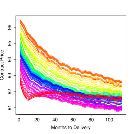
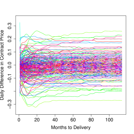
Figure 1: Left hand panel: A rainbow plot of the daily Eurodollar futures curves from 1994 obtained from cubic spline smoothing. Right hand panel: A rainbow plot of the first differenced Eurodollar futures curves. Rainbow plots show earlier curves in red and progresses through the visible spectrum showing later curves in violet.

We considered data spanning 10 years from 1994 to 2003, consisting of approximately 2,500 curves. We treated these data as 10 yearly samples of functional time series each of length approximately 250. The basic question we wish to address in each sample is whether or not the curves in that year seem to exhibit significant serial dependence as measured by their autocovariance operators. We applied the proposed test based on the power-transformed statistic $T_{n}^{\beta_{0}}$ using the Bartlett kernel and corresponding empirical bandwidth of the form $\hat{M}n^{1/3}$ to each sample. The approximate $p$-values of these tests are displayed in the right hand panel of Figure 2, which are essentially equal to zero in all cases. This suggests that the Eurodollar futures curves exhibit substantial serial dependence. This observation is consistent with the suggested FAR(1) model for these curves proposed by Kargin and Onatski, (2008).

Although these results are consistent with the data following an FAR(1) model, they may also be explained by the fact that the raw Eurodollar futures time series are apparently not mean stationary; over periods as long as a year they typically exhibit strong trends and seasonality. We evaluated the stationarity of each of these samples using the test proposed in Horváth et al., (2014), which suggest that in general the raw Eurodollar futures curves are non-stationary. Letting $X_{i}(t)$ denote the futures curve on day $i$, we studied then instead the first order differenced curves $Y_{i}(t)=X_{i}(t)-X_{i-1}(t)$. The first order differenced Eurodollar futures curves from 1994 are shown in the right hand panel of Figure 1, and the stationarity test of Horváth et al., (2014) applied to these curves suggest that they are reasonably stationary. The results of these stationarity tests are illustrated in the left hand panel of Figure 2.

We applied the proposed test using the statistic $T_{n}^{\beta_{0}}$ with the same settings as above to each sample of first differenced curves. In six of the ten years considered the hypothesis that the first differenced futures curves evolve as a functional white noise cannot be rejected at the $0.05$ level. Interestingly however, in consecutive years from 1998 to 2001 the first differenced Eurodollar futures curves exhibit significant autocovariance operators to the $0.05$ level as measured by our tests.

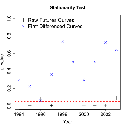
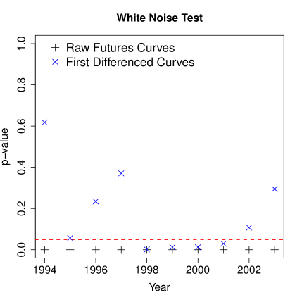
Figure 2: Left hand panel: p-values of the stationarity test proposed in Horváth et al., (2014) against the corresponding year of the sample. Right hand panel: p-values of the proposed white noise test against the corresponding years of the sample. In each figure $+$ corresponds to the raw Eurodollar futures curves, and $\times$ corresponds to the first differenced curves.

5 Conclusion

We have introduced a new test statistic for white noise testing with functional time series based on kernel lag-window estimates of the spectral density operator. The asymptotic properties of the proposed test have been established assuming the observed time series is a strong white noise, and it was also shown to be consistent for general time series exhibiting serial correlation. The test seems to improve upon existing tests in terms of power against functional autoregressive alternatives, although it has the drawback that it is not well sized for general weak white noise sequences in function space, such as for functional GARCH processes.

Based on the work of Shao, 2011b and Shao, 2011a , we conjecture that Theorem 1 can be established for general weakly dependent white noise sequences in $\mathbb{H}$, despite the fact the proposed tests have markedly inflated size for sequences exhibiting conditional heteroscedasticity in our simulation. Roughly speaking, Shao, 2011b shows that in the scalar case the limit distribution of $T_{n}$ is determined asymptotically by the normalized autocovariances of the process at long lags, which behave essentially the same with strong white noise sequences as with weakly dependent white noises. With this in mind and in light of our simulation results, one expects to need very long time series and a large bandwidth in order for this asymptotic result to be predictive of the behavior of the test statistic for general weak white noise sequence exhibiting serial dependence, which encourages the use of a block bootstrap in finite samples. We leave these issues as potential directions for future research.

Appendix

Appendix A Proof of Theorem 1

We begin with a note comparing the basic approach here to that of Horváth et al., (2013). Horváth et al., (2013) uses at its core a central limit theorem for vectors with increasing dimension adapted from Senatov, (1998), and as a result the fairly restrictive condition on the bandwidth $p_{n}=O(\log(n))$ is needed. Our proof is somewhat more straightforward in the sense that we show that the suitably normalized statistic $\hat{Q}_{n}^{2}$ is a martingale with uniformly asymptotically negligible increments. This requires a number of intermediary approximations. Before we prove Theorem 1, we state two elementary lemmas that we use in the proof.

Lemma 1.

Suppose that $X$ and $Y$ are independent random elements with values in a separable Hilbert space $\mathbb{H}$ such that $\operatorname{E}\|X\|<\infty$, $\operatorname{E}\|Y\|<\infty$ and $\operatorname{E}X=0$ or $\operatorname{E}Y=0$. Then $\operatorname{E}\langle X,Y\rangle=0$.

Lemma 2.

Suppose that $X$ and $Y$ are independent and identically distributed random elements with values in a separable Hilbert space $\mathbb{H}$ with zero means and finite second moments. Then

$$\operatorname{E}|\langle X,Y\rangle|^{2}=|\kern-0.96873pt|\kern-0.96873pt|\operatorname{E}[X\otimes X]|\kern-0.96873pt|\kern-0.96873pt|_{2}^{2}.$$

Now we are ready to prove Theorem 1. The basic format of the proof follows Hong, (1996), but in some instances must significantly deviate due to the assumption that the underlying variables are in an arbitrary separable Hilbert space. We denote $k_{nj}=k(j/p_{n})$ and $Z_{jt}=u_{t}\otimes u_{t-j}$.

Proof of Theorem 1.

By (7) and Slutsky’s theorem, it suffices to show that $\hat{\sigma}_{n}^{2}/|\kern-0.96873pt|\kern-0.96873pt|\hat{\mathcal{C}}_{n}(0)|\kern-0.96873pt|\kern-0.96873pt|_{2}\xrightarrow{p}\sigma^{2}/|\kern-0.96873pt|\kern-0.96873pt|\mathcal{C}(0)|\kern-0.96873pt|\kern-0.96873pt|_{2}$ as $n\to\infty$ and

$$\frac{2^{-1}n\hat{\sigma}_{n}^{-4}\hat{Q}_{n}^{2}-C_{n}(k)}{\sqrt{2D_{n}(k)}}\xrightarrow{d}N(0,|\kern-0.96873pt|\kern-0.96873pt|\mathcal{C}(0)|\kern-0.96873pt|\kern-0.96873pt|_{2}^{4}/\sigma^{8})\quad\text{as}\quad n\to\infty.$$ (13)

By the law of large numbers, we have that $\hat{\sigma}_{n}^{2}\xrightarrow{p}\sigma^{2}$ as $n\to\infty$. By Lemma 6 below, $|\kern-0.96873pt|\kern-0.96873pt|\hat{\mathcal{C}}_{n}(0)-\mathcal{C}(0)|\kern-0.96873pt|\kern-0.96873pt|_{2}\xrightarrow{p}0$ as $n\to\infty$ and, using the reverse triangle inequality, $|\kern-0.96873pt|\kern-0.96873pt|\hat{\mathcal{C}}_{n}(0)|\kern-0.96873pt|\kern-0.96873pt|_{2}\xrightarrow{p}|\kern-0.96873pt|\kern-0.96873pt|\mathcal{C}(0)|\kern-0.96873pt|\kern-0.96873pt|_{2}$ as $n\to\infty$. Hence, $\hat{\sigma}_{n}^{2}/|\kern-0.96873pt|\kern-0.96873pt|\hat{\mathcal{C}}_{n}(0)|\kern-0.96873pt|\kern-0.96873pt|_{2}\xrightarrow{p}\sigma^{2}/|\kern-0.96873pt|\kern-0.96873pt|\mathcal{C}(0)|\kern-0.96873pt|\kern-0.96873pt|_{2}$ as $n\to\infty$.

Now we show (13) holds. By Chebyshev’s inequality, $\hat{\sigma}_{n}^{2}-\sigma^{2}=O_{p}(n^{-1/2})$ as $n\to\infty$. Since

$$\operatorname{E}\hat{Q}_{n}^{2}=2\sum_{j=1}^{n-1}k_{jn}^{2}\operatorname{E}|\kern-0.96873pt|\kern-0.96873pt|\hat{\mathcal{C}}_{n}(j)|\kern-0.96873pt|\kern-0.96873pt|_{2}^{2}=2\sigma^{4}n^{-1}\sum_{j=1}^{n-1}(1-j/n)k_{jn}^{2}=2\sigma^{4}n^{-1}C_{n}(k),$$ (14)

Markov’s inequality implies that $\hat{Q}_{n}^{2}=O_{p}(p_{n}/n)$ as $n\to\infty$. We obtain

$$\hat{\sigma}_{n}^{-4}\hat{Q}_{n}^{2}=\sigma^{-4}\hat{Q}_{n}^{2}+(\hat{\sigma}_{n}^{-4}-\sigma^{-4})\hat{Q}_{n}^{2}=\sigma^{-4}\hat{Q}_{n}^{2}+o_{p}(p_{n}^{1/2}/n)\quad\text{as}\quad n\to\infty$$

because $p_{n}/n\to 0$ as $n\to\infty$. Hence,

$$\frac{2^{-1}n\hat{\sigma}_{n}^{-4}\hat{Q}_{n}^{2}-C_{n}(k)}{\sqrt{2D_{n}(k)}}=\frac{2^{-1}n\sigma^{-4}\hat{Q}_{n}^{2}-C_{n}(k)}{\sqrt{2D_{n}(k)}}+o_{p}(1)\quad\text{as}\quad n\to\infty.$$

Since $\hat{\mathcal{C}}_{n}(j)=n^{-1}\sum_{t=j+1}^{n}Z_{jt}$,

$$|\kern-0.96873pt|\kern-0.96873pt|\hat{\mathcal{C}}_{n}(j)|\kern-0.96873pt|\kern-0.96873pt|_{2}^{2}=n^{-2}\sum_{t,s=j+1}^{n}\langle Z_{jt},Z_{js}\rangle_{\mathrm{HS}}=n^{-2}\Big{[}\sum_{t=j+1}^{n}|\kern-0.96873pt|\kern-0.96873pt|Z_{jt}|\kern-0.96873pt|\kern-0.96873pt|_{2}^{2}+\sum_{t=j+2}^{n}\sum_{s=j+1}^{t-1}2\langle Z_{jt},Z_{js}\rangle_{\mathrm{HS}}\Bigr{]}.$$

We obtain

$$2^{-1}n\sigma^{-4}\hat{Q}_{n}^{2}=n\sigma^{-4}\sum_{j=1}^{n-1}k_{jn}^{2}|\kern-0.96873pt|\kern-0.96873pt|\hat{\mathcal{C}}_{n}(j)|\kern-0.96873pt|\kern-0.96873pt|_{2}^{2}=\sigma^{-4}(\tilde{C}_{n}+\tilde{W}_{n}),$$

where

$$\tilde{C}_{n}=n^{-1}\sum_{j=1}^{n-1}\sum_{t=j+1}^{n}k_{nj}^{2}|\kern-0.96873pt|\kern-0.96873pt|Z_{jt}|\kern-0.96873pt|\kern-0.96873pt|_{2}^{2}\quad\text{and}\quad\tilde{W}_{n}=n^{-1}\sum_{j=1}^{n-2}\sum_{t=j+2}^{n}\sum_{s=j+1}^{t-1}2k_{nj}^{2}\langle Z_{jt},Z_{js}\rangle_{\mathrm{HS}}.$$ (15)

Let us observe that

$$\operatorname{E}\tilde{C}_{n}=\sigma^{4}\sum_{j=1}^{n-1}(1-j/n)k_{nj}^{2}=\sigma^{4}C_{n}(k),$$

$$\operatorname{E}|\sigma^{-4}\tilde{C}_{n}-C_{n}(k)|^{2}=\operatorname{E}|\sigma^{-4}\tilde{C}_{n}-\sigma^{-4}\operatorname{E}\tilde{C}_{n}|^{2}=\sigma^{-8}\operatorname{Var}\tilde{C}_{n}$$

and

$$\operatorname{Var}\tilde{C}_{n}=\operatorname{E}|\tilde{C}_{n}-\operatorname{E}\tilde{C}_{n}|^{2}=n^{-2}\operatorname{E}\Bigl{|}\sum_{j=1}^{n-1}k_{nj}^{2}\sum_{t=j+1}^{n}(|\kern-0.96873pt|\kern-0.96873pt|Z_{jt}|\kern-0.96873pt|\kern-0.96873pt|_{2}^{2}-\sigma^{4})\Bigr{|}^{2}.$$

Since $\operatorname{E}|\sum_{t=j+1}^{n}(|\kern-0.96873pt|\kern-0.96873pt|Z_{jt}|\kern-0.96873pt|\kern-0.96873pt|_{2}^{2}-\sigma^{4})|^{2}=O(n)$ as $n\to\infty$ for each $0<j<n$, by Minkowski’s inequality,

$$\operatorname{Var}\tilde{C}_{n}\leq\biggl{|}n^{-1}\sum_{j=1}^{n-1}k_{nj}^{2}\Bigl{(}\operatorname{E}\Bigl{|}\sum_{t=j+1}^{n}(|\kern-0.96873pt|\kern-0.96873pt|Z_{jt}|\kern-0.96873pt|\kern-0.96873pt|_{2}^{2}-\sigma^{4})\Bigr{|}^{2}\Bigr{)}^{1/2}\biggr{|}^{2}=O(p_{n}^{2}/n)\quad\text{as}\quad n\to\infty.$$ (16)

Since $p_{n}/n\to 0$ as $n\to\infty$, we have that $p_{n}^{-1/2}(\sigma^{-4}\tilde{C}_{n}-C_{n}(k))=o_{p}(1)$ as $n\to\infty$ and

$$\frac{2^{-1}n\sigma^{-4}\hat{Q}_{n}^{2}-C_{n}(k)}{\sqrt{2D_{n}(k)}}=\frac{\sigma^{-4}(\tilde{C}_{n}+\tilde{W}_{n})-C_{n}(k)}{\sqrt{2D_{n}(k)}}=\frac{\tilde{W}_{n}}{\sqrt{2\sigma^{8}D_{n}(k)}}+o_{p}(1)\quad\text{as}\quad n\to\infty.$$

So we must show that $\tilde{W}_{n}/\sqrt{2\sigma^{8}D_{n}(k)}\xrightarrow{d}N(0,|\kern-0.96873pt|\kern-0.96873pt|\mathcal{C}(0)|\kern-0.96873pt|\kern-0.96873pt|_{2}^{4}/\sigma^{8})$ as $n\to\infty$. Let us choose a real sequence $\{l_{n}\}_{n\geq 1}$ such that $p_{n}/l_{n}+l_{n}/n\to 0$ as $n\to\infty$. With $w_{jts}=2\langle Z_{jt},Z_{js}\rangle_{\mathrm{HS}}$, we have that

$$\tilde{W}_{n}=\Bigl{[}n^{-1}\sum_{j=1}^{l_{n}}k_{nj}^{2}+n^{-1}\sum_{j=l_{n}+1}^{n-2}k_{nj}^{2}\Bigr{]}\sum_{t=j+2}^{n}\sum_{s=j+1}^{t-1}w_{jts}=W_{1n}+V_{1n}.$$

Next, we partition

$$W_{1n} =n^{-1}\sum_{j=1}^{l_{n}}k_{nj}^{2}\Big{[}\sum_{t=2l_{n}+3}^{n}\sum_{s=l_{n}+2}^{t-l_{n}-1}+\sum_{t=2l_{n}+3}^{n}\sum_{s=t-l_{n}}^{t-1}+\sum_{t=l_{n}+3}^{2l_{n}+2}\sum_{s=l_{n}+2}^{t-1}+\sum_{s=j+1}^{l_{n}+1}\sum_{t=s+1}^{n}\Bigr{]}w_{jts}$$

$$=U_{n}+V_{2n}+V_{3n}+V_{4n}.$$

Hence, $\tilde{W}_{n}=U_{n}+\sum_{j=1}^{4}V_{nj}$. One may show that $p_{n}^{-1/2}V_{jn}=o_{p}(1)$ as $n\to\infty$ for $j=1,\ldots,4$. We provide a complete argument to show $p_{n}^{-1/2}V_{1n}=o_{p}(1)$, and omit the details for $V_{jn}$, $j=2,3$ and 4 since they are similar. We have that

$$|V_{1n}|^{2} =n^{-2}\sum_{j=l_{n}+1}^{n-2}k_{nj}^{4}\biggl{|}\sum_{t=j+2}^{n}\sum_{s=j+1}^{t-1}w_{jts}\biggr{|}^{2}$$

$$\quad+2n^{-2}\sum_{j_{1}=l_{n}+2}^{n-2}\sum_{j_{2}=l_{n}+1}^{n+2}\biggl{(}k_{nj_{1}}^{2}\sum_{t_{1}=j_{1}+2}^{n}\sum_{s_{1}=j_{1}+1}^{t_{1}-1}w_{j_{1}t_{1}s_{1}}\biggr{)}\biggl{(}k_{nj_{2}}^{2}\sum_{t_{2}=j_{2}+2}^{n}\sum_{s_{2}=j_{2}+1}^{t_{2}-1}w_{j_{2}t_{2}s_{2}}\biggr{)}$$

$$=A_{1n}+B_{1n}.$$

Let us consider the expected value $\operatorname{E}[w_{j_{1}t_{1}s_{1}}w_{j_{2}t_{2}s_{2}}]$. If $j_{1}=j_{2}=j$, the expected value is equal to $0$ by Lemma 4 unless $s_{1}=s_{2}$ and $t_{1}=t_{2}$. Hence, using the fact that $\operatorname{E}|w_{jts}|^{2}\leq 4\mu_{4}^{2}$,

$$\operatorname{E}\biggl{|}\sum_{t=j+2}^{n}\sum_{s=j+1}^{t-1}w_{jts}\biggr{|}^{2}=\sum_{t=j+2}^{n}\sum_{s=j+1}^{t-1}\operatorname{E}|w_{jts}|^{2}=O(n^{2})$$

and $\operatorname{E}A_{1n}=o(p_{n})$ since $l_{n}\to\infty$ as $n\to\infty$. Also,

$$\operatorname{E}B_{1n} =2n^{-2}\sum_{j_{1}=l_{n}+2}^{n-2}k_{nj_{1}}^{2}\sum_{j_{2}=l_{n}+1}^{j_{1}-1}k_{nj_{2}}^{2}\bigg{(}\sum_{t_{1}=j_{1}+2}^{n}\sum_{s_{1}=j_{1}+1}^{t_{1}-1}\biggr{)}\bigg{(}\sum_{t_{2}=j_{2}+2}^{n}\sum_{s_{2}=j_{2}+1}^{t_{2}-1}\operatorname{E}[w_{j_{1}t_{1}s_{1}}w_{j_{2}t_{2}s_{2}}]\biggr{)}$$

$$=O(p_{n}^{2}/n)$$

as $n\to\infty$ since $\operatorname{E}[w_{j_{1}t_{1}s_{1}}w_{j_{2}t_{1}s_{2}}]=0$ by Lemma 4 unless $t_{1}=t_{2}$, $s_{1}=t_{1}-j_{2}$ and $s_{2}=t_{1}-j_{1}$ using the fact that $j_{1}>j_{2}$. Hence, $\operatorname{E}|V_{1n}|^{2}=o(p_{n})$ as $n\to\infty$.

Now for $U_{n}$, we have further that

$$U_{n} =n^{-1}\sum_{j=1}^{l_{n}}k_{nj}^{2}\sum_{t=2l_{n}+3}^{n}\sum_{s=l_{n}+2}^{t-l_{n}-1}2\langle Z_{jt},Z_{js}\rangle_{\mathrm{HS}}$$

$$=n^{-1}\sum_{t=2l_{n}+3}^{n}2\sum_{j=1}^{l_{n}}k_{nj}^{2}\Bigl{\langle}Z_{jt},\sum_{s=l_{n}+2}^{t-l_{n}-1}Z_{js}\Bigr{\rangle}_{\mathrm{HS}}$$

$$=n^{-1}\sum_{t=2l_{n}+3}^{n}U_{nt},$$

where

$$U_{nt}=2\sum_{j=1}^{l_{n}}k_{nj}^{2}\langle Z_{jt},H_{jt-l_{n}-1}\rangle_{\mathrm{HS}}\quad\text{and}\quad H_{jt-l_{n}-1}=\sum_{s=l_{n}+2}^{t-l_{n}-1}Z_{js}.$$

To establish the asymptotic distribution of $T_{n}$, we show that $U_{n}/\sqrt{2\sigma^{8}D_{n}(k)}\xrightarrow{d}N(0,|\kern-0.96873pt|\kern-0.96873pt|\mathcal{C}(0)|\kern-0.96873pt|\kern-0.96873pt|_{2}^{4}/\sigma^{8})$ as $n\to\infty$. We have that

$$\operatorname{E}[U_{nt}\mid F_{t-1}] =2\sum_{j=1}^{l_{n}}k_{nj}^{2}\sum_{s=l_{n}+2}^{t-l_{n}-1}\operatorname{E}[\langle u_{t},u_{s}\rangle\langle u_{t-j},u_{s-j}\rangle\mid F_{t-1}]$$

$$=2\sum_{j=1}^{l_{n}}k_{nj}^{2}\sum_{s=l_{n}+2}^{t-l_{n}-1}\langle u_{t-j},u_{s-j}\rangle\operatorname{E}[\langle u_{t},u_{s}\rangle\mid F_{t-1}]$$

using the fact that $\langle u_{t-j},u_{s-j}\rangle$ is $F_{t-1}$-measurable. Suppose that $\{e_{n}\}_{n\geq 1}$ is an orthonormal basis of $\mathbb{H}$. Then

$$\operatorname{E}[\langle u_{t},u_{s}\rangle\mid F_{t-1}]=\sum_{i=1}^{\infty}\operatorname{E}[\langle u_{t},e_{i}\rangle\langle e_{i},u_{s}\rangle\mid F_{t-1}]=\sum_{i=1}^{\infty}\langle e_{i},u_{s}\rangle\operatorname{E}\langle u_{t},e_{i}\rangle=0$$ (17)

using the fact that $\langle e_{i},u_{s}\rangle$ is $F_{t-1}$-measurable. Using the Cauchy-Schwarz inequality, $H_{0,\text{iid}}$, and Parseval’s identity,

$$\sum_{i=1}^{\infty}\operatorname{E}|\langle u_{t},e_{i}\rangle\langle e_{i},u_{s}\rangle|\leq\sum_{i=1}^{\infty}(\operatorname{E}|\langle u_{t},e_{i}\rangle|^{2})^{1/2}(\operatorname{E}|\langle e_{i},u_{s}\rangle|^{2})^{1/2}=\operatorname{E}\|u_{0}\|^{2}<\infty.$$

This shows that the interchange of the expected value and the series in (17) is justified. Hence, $\{U_{nt},F_{t-1}\}$ is a martingale difference sequence, where $F_{t}$ is the $\sigma$-field generated by $u_{s}$, $s\leq t$.

Let us denote $\sigma^{2}(n)=\operatorname{E}U_{n}^{2}$. Theorem 2 of Brown, (1971) states that $\sigma^{-1}(n)U_{n}\xrightarrow{d}N(0,1)$ if both of the following conditions hold:

1. $\sigma^{-2}(n)n^{-2}\sum_{t=2l_{n}+3}^{n}\operatorname{E}[U_{nt}^{2}I_{\{|U_{nt}|>\varepsilon n\sigma(n)\}}]\to 0$ as $n\to\infty$ for each $\varepsilon>0$;

2. $\sigma^{-2}(n)n^{-2}\sum_{t=2l_{n}+3}^{n}\ddot{U}_{nt}^{2}\xrightarrow{p}1$ as $n\to\infty$, where $\ddot{U}_{nt}^{2}=\operatorname{E}[U_{nt}^{2}\mid F_{t-1}]$.

We show that $\sigma^{2}(n)/(2\sigma^{8}p_{n}D(k))\to|\kern-0.96873pt|\kern-0.96873pt|\mathcal{C}(0)|\kern-0.96873pt|\kern-0.96873pt|_{2}^{4}/\sigma^{8}$ as $n\to\infty$. We have that

$$\sigma^{2}(n)=n^{-2}\operatorname{E}\Bigl{|}\sum_{t=2l_{n}+3}^{n}U_{nt}\Bigr{|}^{2}=n^{-2}\Bigl{[}\sum_{t=2l_{n}+3}^{n}\operatorname{E}U_{nt}^{2}+2\sum_{s=2l_{n}+4}^{n}\sum_{t=2l_{n}+3}^{s-1}\operatorname{E}[U_{ns}U_{nt}]\Bigr{]}.$$

Let us observe that $Z_{it}=u_{t}\otimes u_{t-i}$ is independent of $H_{jt-l_{n}-1}=\sum_{s=l_{n}+2}^{t-l_{n}-1}u_{s}\otimes u_{s-j}$ for $2l_{n}+3\leq t\leq n$ and $1\leq i,j\leq l_{n}$. We obtain

$$\operatorname{E}U_{nt}^{2}=4\sum_{j=1}^{l_{n}}k_{nj}^{4}\operatorname{E}|\langle Z_{jt},H_{jt-l_{n}-1}\rangle_{\mathrm{HS}}|^{2}\\ +8\sum_{j=2}^{l_{n}}\sum_{i=1}^{j-1}k_{nj}^{2}k_{ni}^{2}\operatorname{E}[\langle Z_{jt},H_{jt-l_{n}-1}\rangle_{\mathrm{HS}}\langle Z_{it},H_{it-l_{n}-1}\rangle_{\mathrm{HS}}].$$

We have that

$$\operatorname{E}|\langle Z_{jt},H_{jt-l_{n}-1}\rangle_{\mathrm{HS}}|^{2}=\sum_{s=l_{n}+2}^{t-l_{n}-1}\operatorname{E}|\langle Z_{jt},Z_{js}\rangle_{\mathrm{HS}}|^{2}+2\sum_{s=l_{n}+3}^{t-l_{n}-1}\sum_{r=l_{n}+2}^{s-1}\operatorname{E}[\langle Z_{jt},Z_{js}\rangle_{\mathrm{HS}}\langle Z_{jt},Z_{jr}\rangle_{\mathrm{HS}}].$$

Let us notice that $u_{t}$, $u_{t-j}$, $u_{s}$ and $u_{s-j}$ are independent random elements for $2l_{n}+3\leq t\leq n$, $l_{n}+2\leq s\leq t-l_{n}-1$ and $1\leq j\leq l_{n}$. Hence, $\langle u_{t},u_{s}\rangle$ and $\langle u_{s-j},u_{t-j}\rangle$ are independent as well and

$$\operatorname{E}|\langle Z_{jt},Z_{js}\rangle_{\mathrm{HS}}|^{2}=\operatorname{E}|\langle u_{t},u_{s}\rangle\langle u_{s-j},u_{t-j}\rangle|^{2}=\operatorname{E}|\langle u_{t},u_{s}\rangle|^{2}\operatorname{E}|\langle u_{s-j},u_{t-j}\rangle|^{2}=|\kern-0.96873pt|\kern-0.96873pt|\mathcal{C}(0)|\kern-0.96873pt|\kern-0.96873pt|_{2}^{4}$$

by Lemma 2. Since $r-j<s-j$,

$$\operatorname{E}[\langle Z_{jt},Z_{js}\rangle_{\mathrm{HS}}\langle Z_{jt},Z_{jr}\rangle_{\mathrm{HS}}]=\operatorname{E}\langle u_{r-j},\langle u_{s},u_{t}\rangle\langle u_{t-j},u_{s-j}\rangle\langle u_{r},u_{t}\rangle u_{t-j}\rangle=0$$

using Lemma 1. Since $i<j$,

$$\operatorname{E}[\langle Z_{jt},H_{jt-l_{n}-1}\rangle_{\mathrm{HS}}\langle Z_{it},H_{it-l_{n}-1}\rangle_{\mathrm{HS}}]=\\ =\sum_{s=l_{n}+2}^{t-l_{n}-1}\sum_{r=l_{n}+2}^{t-l_{n}-1}\operatorname{E}\langle\langle u_{t},u_{s}\rangle\langle u_{s-j},u_{t-j}\rangle\langle u_{t},u_{r}\rangle u_{r-i},u_{t-i}\rangle=0.$$

Finally,

$$\operatorname{E}[U_{ns}U_{nt}] =4\operatorname{E}\bigg{[}\Big{[}\sum_{i=1}^{l_{n}}k_{ni}^{2}\langle Z_{is},H_{is-l_{n}-1}\rangle_{\mathrm{HS}}\Bigr{]}\Bigl{[}\sum_{j=1}^{l_{n}}k_{nj}^{2}\langle Z_{jt},H_{jt-l_{n}-1}\rangle_{\mathrm{HS}}\Bigr{]}\biggr{]}$$

$$=4\sum_{i=1}^{l_{n}}\sum_{j=1}^{l_{n}}k_{ni}^{2}k_{nj}^{2}\operatorname{E}[\langle Z_{is},H_{is-l_{n}-1}\rangle_{\mathrm{HS}}\langle Z_{jt},H_{jt-l_{n}-1}\rangle_{\mathrm{HS}}]$$

and

$$\operatorname{E}[\langle Z_{is},H_{is-l_{n}-1}\rangle_{\mathrm{HS}}\langle Z_{jt},H_{jt-l_{n}-1}\rangle_{\mathrm{HS}}] =\sum_{r=l_{n}+2}^{s-l_{n}-1}\sum_{v=l_{n}+2}^{t-l_{n}-1}\operatorname{E}[\langle Z_{is},Z_{ir}\rangle_{\mathrm{HS}}\langle Z_{jt},Z_{jv}\rangle_{\mathrm{HS}}]$$

$$=\sum_{r=l_{n}+2}^{s-l_{n}-1}\sum_{v=l_{n}+2}^{t-l_{n}-1}\operatorname{E}\langle u_{s},\langle u_{r-i},u_{s-i}\rangle\langle u_{t},u_{v}\rangle\langle u_{v-j},u_{t-j}\rangle u_{r}\rangle$$

$$=0$$

since $t<s$. Hence,

$$\sigma^{2}(n)=2|\kern-0.96873pt|\kern-0.96873pt|\mathcal{C}(0)|\kern-0.96873pt|\kern-0.96873pt|_{2}^{4}n^{-2}(n-2l_{n}-2)(n-2l_{n}-1)\sum_{j=1}^{l_{n}}k_{nj}^{4}$$ (18)

and $\sigma^{2}(n)/(2\sigma^{8}p_{n}D(k))\to|\kern-0.96873pt|\kern-0.96873pt|\mathcal{C}(0)|\kern-0.96873pt|\kern-0.96873pt|_{2}^{4}/\sigma^{8}$ as $n\to\infty$.

We show that (a) holds. We have that

$$\operatorname{E}|U_{nt}|^{4}\leq 48\Bigl{|}\sum_{j=1}^{l_{n}}k_{nj}^{4}(\operatorname{E}|\langle Z_{jt},H_{jt-l_{n}-1}\rangle_{\mathrm{HS}}|^{4})^{1/2}\Bigr{|}^{2}$$

since

$$\operatorname{E}\Bigl{|}\sum_{j=1}^{l_{n}}k_{nj}^{2}\langle Z_{jt},H_{jt-l_{n}-1}\rangle_{\mathrm{HS}}\Bigr{|}^{4}=\sum_{j=1}^{l_{n}}k_{nj}^{8}\operatorname{E}|\langle Z_{jt},H_{jt-l_{n}-1}\rangle_{\mathrm{HS}}|^{4}\\ +6\sum_{j=2}^{l_{n}}\sum_{i=1}^{j-1}k_{nj}^{4}k_{ni}^{4}\operatorname{E}|\langle Z_{jt},H_{jt-l_{n}-1}\rangle_{\mathrm{HS}}\langle Z_{it},H_{it-l_{n}-1}\rangle_{\mathrm{HS}}|^{2}$$

and

$$\operatorname{E}|\langle Z_{jt},H_{jt-l_{n}-1}\rangle_{\mathrm{HS}}\langle Z_{it},H_{it-l_{n}-1}\rangle_{\mathrm{HS}}|^{2}\\ \leq(\operatorname{E}|\langle Z_{jt},H_{jt-l_{n}-1}\rangle_{\mathrm{HS}}|^{4})^{1/2}(\operatorname{E}|\langle Z_{it},H_{it-l_{n}-1}\rangle_{\mathrm{HS}}|^{4})^{1/2}$$

by the Cauchy-Schwarz inequality. Again by the Cauchy-Schwarz inequality and independence of $u_{t}$’s,

$$\operatorname{E}|\langle Z_{jt},H_{jt-l_{n}-1}\rangle_{\mathrm{HS}}|^{4}\leq\operatorname{E}||\kern-0.96873pt|\kern-0.96873pt|Z_{jt}|\kern-0.96873pt|\kern-0.96873pt|_{2}|\kern-0.96873pt|\kern-0.96873pt|H_{jt-l_{n}-1}|\kern-0.96873pt|\kern-0.96873pt|_{2}|^{4}=(\operatorname{E}\|u_{0}\|^{4})^{2}\operatorname{E}|\kern-0.96873pt|\kern-0.96873pt|H_{jt-l_{n}-1}|\kern-0.96873pt|\kern-0.96873pt|_{2}^{4}.$$

Also,

$$\operatorname{E}|\kern-0.96873pt|\kern-0.96873pt|H_{jt-l_{n}-1}|\kern-0.96873pt|\kern-0.96873pt|_{2}^{4}=\operatorname{E}\Big{|}\sum_{s=l_{n}+2}^{t-l_{n}-1}\sum_{r=l_{n}+2}^{t-l_{n}-1}\langle Z_{js},Z_{jr}\rangle_{\mathrm{HS}}\Bigr{|}^{2}=O(t^{2}).$$ (19)

Hence, $\operatorname{E}|U_{nt}|^{4}=O(p_{n}^{2}t^{2})$ and $\sigma^{-4}(n)n^{-4}\sum_{t=2l_{n}+3}^{n}\operatorname{E}U_{nt}^{4}=O(n^{-1})$.

Now we move to the proof of (b). Let us denote $\ddot{U}_{n}^{2}=n^{-2}\sum_{t=2l_{n}+3}^{n}\ddot{U}_{nt}^{2}$. We show that $\sigma^{-2}(n)[\ddot{U}_{nt}^{2}-\sigma^{2}(n)]\xrightarrow{p}0$ by showing that $\sigma^{-4}(n)\operatorname{E}|\ddot{U}_{n}^{2}-\sigma^{2}(n)|^{2}\to 0$ as $n\to\infty$. We have that

$$\ddot{U}_{nt}^{2} =4\sum_{j=1}^{l_{n}}k_{nj}^{4}\operatorname{E}[|\langle Z_{jt},H_{jt-l_{n}-1}\rangle_{\mathrm{HS}}|^{2}\mid F_{t-1}]$$

$$\quad+8\sum_{j=2}^{l_{n}}\sum_{i=1}^{j-1}k_{nj}^{2}k_{ni}^{2}\operatorname{E}[\langle Z_{jt},H_{jt-l_{n}-1}\rangle_{\mathrm{HS}}\langle Z_{it},H_{it-l_{n}-1}\rangle_{\mathrm{HS}}\mid F_{t-1}]$$

$$=4B_{nt}+4A_{1nt}.$$

Since

$$\operatorname{E}[|\langle Z_{jt},H_{jt-l_{n}-1}\rangle_{\mathrm{HS}}|^{2}\mid F_{t-1}]=\sum_{s=l_{n}+2}^{t-l_{n}-1}\operatorname{E}[|\langle Z_{jt},Z_{js}\rangle_{\mathrm{HS}}|^{2}\mid F_{t-1}]\\ +2\sum_{s=l_{n}+3}^{t-l_{n}-1}\sum_{r=l_{n}+2}^{s-1}\operatorname{E}[\langle Z_{jt},Z_{js}\rangle_{\mathrm{HS}}\langle Z_{jt},Z_{jr}\rangle_{\mathrm{HS}}\mid F_{t-1}],$$

$$B_{nt} =\sum_{j=1}^{l_{n}}k_{nj}^{4}\bigg{[}\sum_{s=l_{n}+2}^{t-l_{n}-1}\operatorname{E}[|\langle Z_{jt},Z_{js}\rangle_{\mathrm{HS}}|^{2}\mid F_{t-1}]\biggr{]}$$

$$\quad+\sum_{j=1}^{l_{n}}k_{nj}^{4}\bigg{[}2\sum_{s=l_{n}+3}^{t-l_{n}-1}\sum_{r=l_{n}+2}^{s-1}\operatorname{E}[\langle Z_{jt},Z_{js}\rangle_{\mathrm{HS}}\langle Z_{jt},Z_{jr}\rangle_{\mathrm{HS}}\mid F_{t-1}]\biggr{]}$$

$$=C_{nt}+A_{2nt}.$$

Finally,

$$C_{nt} =\sum_{j=1}^{l_{n}}k_{nj}^{4}\bigg{[}\sum_{s=l_{n}+2}^{t-l_{n}-1}(\operatorname{E}[|\langle Z_{jt},Z_{js}\rangle_{\mathrm{HS}}|^{2}\mid F_{t-1}]-|\kern-0.96873pt|\kern-0.96873pt|\mathcal{C}(0)|\kern-0.96873pt|\kern-0.96873pt|_{2}^{4})\biggr{]}+|\kern-0.96873pt|\kern-0.96873pt|\mathcal{C}(0)|\kern-0.96873pt|\kern-0.96873pt|_{2}^{4}(t-2l_{n}-2)\sum_{j=1}^{l_{n}}k_{nj}^{4}$$

$$=A_{3nt}+|\kern-0.96873pt|\kern-0.96873pt|\mathcal{C}(0)|\kern-0.96873pt|\kern-0.96873pt|_{2}^{4}(t-2l_{n}-2)\sum_{j=1}^{l_{n}}k_{nj}^{4}.$$

Hence,

$$\ddot{U}_{n}^{2} =2|\kern-0.96873pt|\kern-0.96873pt|\mathcal{C}(0)|\kern-0.96873pt|\kern-0.96873pt|_{2}^{4}n^{-2}(n-2l_{n}-2)(n-2l_{n}-1)\sum_{j=1}^{l_{n}}k_{nj}^{4}+4n^{-2}\sum_{t=2l_{n}+3}^{n}\sum_{j=1}^{3}A_{jnt}$$

$$=\sigma^{2}(n)+4n^{-2}\sum_{t=2l_{n}+3}^{n}\sum_{j=1}^{3}A_{jnt}$$

using (18) and $\ddot{U}_{n}^{2}-\sigma^{2}(n)=4n^{-2}\sum_{t=2l_{n}+3}^{n}\sum_{j=1}^{3}A_{jnt}$.

Now we show that $\sigma^{-4}(n)n^{-4}\operatorname{E}|\sum_{t=2l_{n}+3}^{n}A_{jnt}|^{2}\to 0$ as $n\to\infty$ for $j=1,2,3$. First, we establish that $n^{-4}\operatorname{E}|\sum_{t=2l_{n}+3}^{n}A_{1nt}|^{2}=o(p_{n}^{2})$ as $n\to\infty$. We have that

$$\operatorname{E}[\langle Z_{jt},H_{jt-l_{n}-1}\rangle_{\mathrm{HS}}\langle Z_{it},H_{it-l_{n}-1}\rangle_{\mathrm{HS}}\mid F_{t-1}]\\ =\sum_{s=l_{n}+2}^{t-l_{n}-1}\sum_{v=l_{n}+2}^{t-l_{n}-1}\langle u_{s-j},u_{t-j}\rangle\langle u_{v-i},u_{t-i}\rangle\operatorname{E}[\langle u_{t},u_{s}\rangle\langle u_{t},u_{v}\rangle\mid F_{t-1}].$$ (20)

The largest index of $u_{t}$’s in (20) is $t-i$ ($t-i>t-j$ since $j>i$ in the expression of $A_{1nt}$; $t-i$ is greater than $s-j$, $v-i$, $s$ and $v$ since $t-i\geq t-l_{n}+1$ while $s-j\leq t-l_{n}-3$, $v-i\leq t-l_{n}-2$; $s\leq t-l_{n}-1$ and $v\leq t-l_{n}-1$). The second largest index is $t-j$ and it does not coincide with any other indices ($t-j$ is greater than $s-j$, $v-i$, $s$ and $v$ since $t-j\geq t-l_{n}$ while $s-j\leq t-l_{n}-3$, $v-i\leq t-l_{n}-2$, $s\leq t-l_{n}-1$ and $v\leq t-l_{n}-1$). Together with Lemma 1, this implies that

$$\operatorname{E}[\operatorname{E}[\langle Z_{j_{1}t},H_{j_{1}t-l_{n}-1}\rangle_{\mathrm{HS}}\langle Z_{i_{1}t},H_{i_{1}t-l_{n}-1}\rangle_{\mathrm{HS}}\mid F_{t-1}]\\ \times\operatorname{E}[\langle Z_{j_{2}t},H_{j_{2}t-l_{n}-1}\rangle_{\mathrm{HS}}\langle Z_{i_{2}t},H_{i_{2}t-l_{n}-1}\rangle_{\mathrm{HS}}\mid F_{t-1}]]=0$$

if $i_{1}\neq i_{2}$ or $j_{1}\neq j_{2}$. Hence,

$$\operatorname{E}A_{1nt}^{2}=4\sum_{j=2}^{l_{n}}\sum_{i=1}^{j-1}k_{nj}^{4}k_{ni}^{4}\operatorname{E}|\operatorname{E}[\langle Z_{jt},H_{jt-l_{n}-1}\rangle_{\mathrm{HS}}\langle Z_{it},H_{it-l_{n}-1}\rangle_{\mathrm{HS}}\mid F_{t-1}]|^{2}.$$

Using the Cauchy-Schwarz inequality twice, the fact that $u_{t}$’s are independent and that $F_{t}$ is the $\sigma$-field consisting of $u_{s}$, $s\leq t$,

$$\operatorname{E}\bigl{|}\operatorname{E}[\langle Z_{jt},H_{jt-l_{n}-1}\rangle_{\mathrm{HS}}\langle Z_{it},H_{it-l_{n}-1}\rangle_{\mathrm{HS}}\mid F_{t-1}]\bigr{|}^{2}\leq$$

$$\leq\operatorname{E}\bigl{|}\operatorname{E}[\|u_{t}\|\|u_{t-j}\||\kern-0.96873pt|\kern-0.96873pt|H_{jt-l_{n}-1}|\kern-0.96873pt|\kern-0.96873pt|_{2}\|u_{t}\|\|u_{t-i}\||\kern-0.96873pt|\kern-0.96873pt|H_{it-l_{n}-1}|\kern-0.96873pt|\kern-0.96873pt|_{2}\mid F_{t-1}]\bigr{|}^{2}$$

$$=\sigma^{8}\operatorname{E}\bigl{|}|\kern-0.96873pt|\kern-0.96873pt|H_{jt-l_{n}-1}|\kern-0.96873pt|\kern-0.96873pt|_{2}|\kern-0.96873pt|\kern-0.96873pt|H_{it-l_{n}-1}|\kern-0.96873pt|\kern-0.96873pt|_{2}\bigr{|}^{2}$$

$$\leq\sigma^{8}(\operatorname{E}|\kern-0.96873pt|\kern-0.96873pt|H_{jt-l_{n}-1}|\kern-0.96873pt|\kern-0.96873pt|_{2}^{4})^{1/2}(\operatorname{E}|\kern-0.96873pt|\kern-0.96873pt|H_{it-l_{n}-1}|\kern-0.96873pt|\kern-0.96873pt|_{2}^{4})^{1/2}.$$

Using (19), we conclude that $\operatorname{E}A_{1nt}^{2}=O(p_{n}^{2}t^{2})$. Since the largest index of $u_{t}$’s in $A_{1nt}$ is $t-i$, $\operatorname{E}[A_{1nt}A_{1ns}]=0$ if $t-l_{n}>s-1$. Hence, using the Cauchy-Schwarz inequality and the fact that $\sum_{|t-s|\leq l_{n}}ts=O(l_{n}n^{3})$,

$$\operatorname{E}\biggl{|}\sum_{t=2l_{n}+3}^{n}A_{1nt}\biggr{|}^{2}=\sum_{|t-s|\leq l_{n}}\operatorname{E}[A_{1nt}A_{1ns}]\leq\sum_{|t-s|\leq l_{n}}(\operatorname{E}A_{1nt}^{2})^{1/2}(\operatorname{E}A_{1ns}^{2})^{1/2}=O(p_{n}^{2}l_{n}n^{3})$$

and, since $l_{n}/n\to 0$, $n^{-4}\operatorname{E}|\sum_{t=2l_{n}+3}^{n}A_{1nt}|^{2}=o(p_{n}^{2})$ as $n\to\infty$.

We establish that $n^{-4}\operatorname{E}|\sum_{t=2l_{n}+3}^{n}A_{2nt}|^{2}=O(p_{n})$ as $n\to\infty$. Let us observe that

$$\operatorname{E}A_{2nt}^{2}=\sum_{j=1}^{l_{n}}k_{nj}^{8}\operatorname{E}\bigg{|}2\sum_{s=l_{n}+3}^{t-l_{n}-1}\sum_{r=l_{n}+2}^{s-1}\operatorname{E}[\langle Z_{jt},Z_{js}\rangle_{\mathrm{HS}}\langle Z_{jt},Z_{jr}\rangle_{\mathrm{HS}}\mid F_{t-1}]\biggr{|}^{2}\\ +2\sum_{j_{1}=2}^{l_{n}}\sum_{j_{2}=1}^{j_{1}-1}k_{nj_{1}}^{4}k_{nj_{2}}^{4}\operatorname{E}\biggl{(}\bigg{[}2\sum_{s_{1}=l_{n}+3}^{t-l_{n}-1}\sum_{r_{1}=l_{n}+2}^{s_{1}-1}\operatorname{E}[\langle Z_{j_{1}t},Z_{j_{1}s_{1}}\rangle_{\mathrm{HS}}\langle Z_{j_{1}t},Z_{j_{1}r_{1}}\rangle_{\mathrm{HS}}\mid F_{t-1}]\biggr{]}\\ \times\bigg{[}2\sum_{s_{2}=l_{n}+3}^{t-l_{n}-1}\sum_{r_{2}=l_{n}+2}^{s_{2}-1}\operatorname{E}[\langle Z_{j_{2}t},Z_{j_{2}s_{2}}\rangle_{\mathrm{HS}}\langle Z_{j_{2}t},Z_{j_{2}r_{2}}\rangle_{\mathrm{HS}}\mid F_{t-1}]\biggr{]}\biggr{)}.$$ (21)

We have that

$$\operatorname{E}[\langle Z_{jt},Z_{js}\rangle_{\mathrm{HS}}\langle Z_{jt},Z_{jr}\rangle_{\mathrm{HS}}\mid F_{t-1}]=\langle u_{s-j},u_{t-j}\rangle\langle u_{r-j},u_{t-j}\rangle\operatorname{E}[\langle u_{t},u_{s}\rangle\langle u_{t},u_{r}\rangle\mid F_{t-1}],$$

where $t-j>s>s-j\lessgtr r>r-j$. Consequently, using Lemma 1,

$$\operatorname{E}\bigl{(}\langle u_{s_{1}-j},u_{t-j}\rangle\langle u_{r_{1}-j},u_{t-j}\rangle\operatorname{E}[\langle u_{t},u_{s_{1}}\rangle\langle u_{t},u_{r_{1}}\rangle\mid F_{t-1}]\\ \times\langle u_{s_{2}-j},u_{t-j}\rangle\langle u_{r_{2}-j},u_{t-j}\rangle\operatorname{E}[\langle u_{t},u_{s_{2}}\rangle\langle u_{t},u_{r_{2}}\rangle\mid F_{t-1}]\bigr{)}=0$$

if $r_{1}\neq r_{2}$ or $s_{1}\neq s_{2}$. It follows that

$$\operatorname{E}\bigg{|}2\sum_{s=l_{n}+3}^{t-l_{n}-1}\sum_{r=l_{n}+2}^{s-1}\operatorname{E}[\langle Z_{jt},Z_{js}\rangle_{\mathrm{HS}}\langle Z_{jt},Z_{jr}\rangle_{\mathrm{HS}}\mid F_{t-1}]\biggr{|}^{2}\\ =4\sum_{s=l_{n}+3}^{t-l_{n}-1}\sum_{r=l_{n}+2}^{s-1}\operatorname{E}|\operatorname{E}[\langle Z_{jt},Z_{js}\rangle_{\mathrm{HS}}\langle Z_{jt},Z_{jr}\rangle_{\mathrm{HS}}\mid F_{t-1}]|^{2}\leq 4\sigma^{8}\mu^{2}{t-2l_{n}-2\choose 2}=O(t^{2})$$

as $t\to\infty$. We now investigate

$$\operatorname{E}\bigl{[}\langle u_{s_{1}-j_{1}},u_{t-j_{1}}\rangle\langle u_{r_{1}-j_{1}},u_{t-j_{1}}\rangle\operatorname{E}[\langle u_{t},u_{s_{1}}\rangle\langle u_{t},u_{r_{1}}\rangle\mid F_{t-1}]\\ \times\langle u_{s_{2}-j_{2}},u_{t-j_{2}}\rangle\langle u_{r_{2}-j_{2}},u_{t-j_{2}}\rangle\operatorname{E}[\langle u_{t},u_{s_{2}}\rangle\langle u_{t},u_{r_{2}}\rangle\mid F_{t-1}]\bigr{]},$$ (22)

where $t-j_{1}>s_{1}>s_{1}-j_{1}\lessgtr r_{1}>r_{1}-j_{1}$ and $t-j_{2}>s_{2}>s_{2}-j_{2}\lessgtr r_{2}>r_{2}-j_{2}$. If $r_{1}-j_{1}\neq r_{2}-j_{2}$, the expected value in (22) is equal to $0$. Thus, we assume that $r_{1}-j_{1}=r_{2}-j_{2}$ (this implies that $r_{1}>r_{2}$ since $j_{1}>j_{2}$). Also, $r_{2}=r_{1}-j_{1}+j_{2}>r_{1}-j_{1}$. Hence, the expected value is equal to $0$ if $r_{2}\neq s_{2}-j_{2}$. We assume that $r_{2}=s_{2}-j_{2}$ ($s_{2}=r_{2}+j_{2}=r_{1}-j_{1}+2j_{2}$). Since $t-j_{2}\geq t-l_{n}+1$ and $r_{1}\leq t-l_{n}-2$, $r_{1}=r_{1}-j_{1}+2j_{2}$, which implies that $j_{1}=2j_{2}$ or $r_{1}=s_{1}-j_{1}$. Otherwise the expected in (22) value is equal to $0$. We conclude that the second term on the right hand side of (21) is $O(p_{n}^{2}t+p_{n}t^{2})$, $\operatorname{E}A_{2nt}^{2}=O(p_{n}t^{2}+p_{n}^{2}t)$ and, by Minkowski’s inequality,

$$n^{-4}\operatorname{E}\biggl{|}\sum_{t=2l_{n}+3}^{n}A_{2nt}\biggr{|}^{2}\leq n^{-4}\operatorname{E}\biggl{|}\sum_{t=2l_{n}+3}^{n}(\operatorname{E}A_{2nt}^{2})^{1/2}\biggr{|}^{2}=O(p_{n})\quad\text{as}\quad n\to\infty.$$

Lastly, we show that $n^{-4}\operatorname{E}|\sum_{t=2l_{n}+3}^{n}A_{3nt}|^{2}=o(p_{n}^{2})$ as $n\to\infty$. We have that

$$n^{-4}\operatorname{E}\bigg{|}\sum_{t=2l_{n}+3}^{n}A_{3nt}\biggr{|}^{2}=n^{-4}\sum_{t=2l_{n}+3}^{n}\operatorname{E}A_{3nt}^{2}+2n^{-4}\sum_{t_{1}=2l_{n}+4}^{n}\sum_{t_{2}=2l_{n}+3}^{t_{1}-1}\operatorname{E}[A_{3nt_{1}}A_{3nt_{2}}].$$ (23)

Since $\operatorname{E}[|\langle Z_{jt},Z_{js}\rangle_{\mathrm{HS}}|^{2}\mid F_{t-1}]=|\kern-0.96873pt|\kern-0.96873pt|\mathcal{C}(0)|\kern-0.96873pt|\kern-0.96873pt|_{2}^{4}$ (see Lemma 3 below), we obtain

$$\operatorname{E}A_{3nt}^{2}=\sum_{j=1}^{l_{n}}k_{nj}^{8}\operatorname{E}\bigg{|}\sum_{s=l_{n}+2}^{t-l_{n}-1}(\operatorname{E}[|\langle Z_{jt},Z_{js}\rangle_{\mathrm{HS}}|^{2}\mid F_{t-1}]-|\kern-0.96873pt|\kern-0.96873pt|\mathcal{C}(0)|\kern-0.96873pt|\kern-0.96873pt|_{2}^{4})\biggr{|}^{2}+2\sum_{j_{1}=2}^{l_{n}}\sum_{j_{2}=1}^{j_{1}-1}k_{nj_{1}}^{4}k_{nj_{2}}^{4}\\ \times\sum_{s_{1}=l_{n}+2}^{t-l_{n}-1}\sum_{s_{2}=l_{n}+2}^{t-l_{n}-1}\operatorname{Cov}[\operatorname{E}[|\langle Z_{j_{1}t},Z_{j_{1}s_{1}}\rangle_{\mathrm{HS}}|^{2}\mid F_{t-1}],\operatorname{E}[|\langle Z_{j_{2}t},Z_{j_{2}s_{2}}\rangle_{\mathrm{HS}}|^{2}\mid F_{t-1}]]$$

and

$$\operatorname{E}\bigg{|}\sum_{s=l_{n}+2}^{t-l_{n}-1}(\operatorname{E}[|\langle Z_{jt},Z_{js}\rangle_{\mathrm{HS}}|^{2}\mid F_{t-1}]-|\kern-0.96873pt|\kern-0.96873pt|\mathcal{C}(0)|\kern-0.96873pt|\kern-0.96873pt|_{2}^{4})\biggr{|}^{2}=\sum_{s=l_{n}+2}^{t-l_{n}-1}\operatorname{Var}[\operatorname{E}[|\langle Z_{jt},Z_{js}\rangle_{\mathrm{HS}}|^{2}\mid F_{t-1}]]\\ \qquad+2\sum_{s=l_{n}+3}^{t-l_{n}-1}\sum_{r=l_{n}+2}^{s-1}\operatorname{Cov}[\operatorname{E}[|\langle Z_{jt},Z_{js}\rangle_{\mathrm{HS}}|^{2}\mid F_{t-1}],\operatorname{E}[|\langle Z_{jt},Z_{jr}\rangle_{\mathrm{HS}}|^{2}\mid F_{t-1}]].$$

Using the Cauchy-Schwarz inequality, the fact that $u_{t}$ is independent of $F_{t-1}$, $u_{t-j}$, $u_{s}$ and $u_{s-j}$ are $F_{t-1}$-measurable and the independence of $u_{t}$’s (let us observe that $t-j\geq t-l_{n}$ and $s\leq t-l_{n}-1$),

$$\operatorname{E}|\operatorname{E}[|\langle Z_{jt},Z_{js}\rangle_{\mathrm{HS}}|^{2}\mid F_{t-1}]|^{2}\leq\operatorname{E}|\operatorname{E}[\|u_{t}\|^{2}\|u_{t-j}\|^{2}\|u_{s}\|^{2}\|u_{s-j}\|^{2}\mid F_{t-1}]|^{2}=\sigma^{4}\mu_{4}^{3}<\infty.$$

Since

$$\operatorname{Var}[\operatorname{E}[|\langle Z_{jt},Z_{js}\rangle_{\mathrm{HS}}|^{2}\mid F_{t-1}]]\leq\operatorname{E}|\operatorname{E}[|\langle Z_{jt},Z_{js}\rangle_{\mathrm{HS}}|^{2}\mid F_{t-1}]|^{2}\\ \leq\sigma^{4}\mu_{4}^{3}$$ (24)

we obtain $\sum_{s=l_{n}+2}^{t-l_{n}-1}\operatorname{Var}[\operatorname{E}[|\langle Z_{jt},Z_{js}\rangle_{\mathrm{HS}}|^{2}\mid F_{t-1}]]=O(t)$ as $t\to\infty$. Using the fact that

$$|\operatorname{Cov}[\operatorname{E}[|\langle Z_{jt},Z_{js}\rangle_{\mathrm{HS}}|^{2}\mid F_{t-1}],\operatorname{E}[|\langle Z_{jt},Z_{jr}\rangle_{\mathrm{HS}}|^{2}\mid F_{t-1}]]|\\ \leq(\operatorname{Var}[\operatorname{E}[|\langle Z_{jt},Z_{js}\rangle_{\mathrm{HS}}|^{2}\mid F_{t-1}]])^{1/2}(\operatorname{Var}[\operatorname{E}[|\langle Z_{jt},Z_{jr}\rangle_{\mathrm{HS}}|^{2}\mid F_{t-1}]])^{1/2}\leq\sigma^{4}\mu_{4}^{3},$$

we obtain

$$2\sum_{s=l_{n}+3}^{t-l_{n}-1}\sum_{r=l_{n}+2}^{s-1}|\operatorname{Cov}[\operatorname{E}[|\langle Z_{jt},Z_{js}\rangle_{\mathrm{HS}}|^{2}\mid F_{t-1}],\operatorname{E}[|\langle Z_{jt},Z_{jr}\rangle_{\mathrm{HS}}|^{2}\mid F_{t-1}]]|\\ \leq 2\sigma^{4}\mu_{4}^{3}\sum_{s=l_{n}+3}^{t-l_{n}-1}(s-l_{n}-2)=\sigma^{4}\mu_{4}^{3}(t-2l_{n}-2)(t-2l_{n}-3)=O(t^{2})$$

as $t\to\infty$. We have that

$$2\sum_{j_{1}=2}^{l_{n}}\sum_{j_{2}=1}^{j_{1}-1}k_{nj_{1}}^{4}k_{nj_{2}}^{4}\sum_{s_{1}=l_{n}+2}^{t-l_{n}-1}\sum_{s_{2}=l_{n}+2}^{t-l_{n}-1}\operatorname{Cov}(\operatorname{E}[|\langle Z_{j_{1}t},Z_{j_{1}s_{1}}\rangle_{\mathrm{HS}}|^{2}\mid F_{t-1}],\operatorname{E}[|\langle Z_{j_{2}t},Z_{j_{2}s_{2}}\rangle_{\mathrm{HS}}|^{2}\mid F_{t-1}])=$$

$$=O(p_{n}^{2}t^{2})$$

since

$$\operatorname{Cov}(\operatorname{E}[|\langle Z_{j_{1}t},Z_{j_{1}s_{1}}\rangle_{\mathrm{HS}}|^{2}\mid F_{t-1}],\operatorname{E}[|\langle Z_{j_{2}t},Z_{j_{2}s_{2}}\rangle_{\mathrm{HS}}|^{2}\mid F_{t-1}])\\ \leq(\operatorname{Var}[\operatorname{E}[|\langle Z_{j_{1}t},Z_{j_{1}s_{1}}\rangle_{\mathrm{HS}}|^{2}\mid F_{t-1}]])^{1/2}(\operatorname{Var}[\operatorname{E}[|\langle Z_{j_{2}t},Z_{j_{2}s_{2}}\rangle_{\mathrm{HS}}|^{2}\mid F_{t-1}]])^{1/2}\leq\sigma^{4}\mu_{4}^{3}.$$

Now we bound the second term on the right hand side of (23). We have that

$$\operatorname{E}[A_{3nt_{1}}A_{3nt_{2}}]=\sum_{j_{1}=1}^{l_{n}}k_{nj_{1}}^{4}\sum_{j_{2}=1}^{l_{n}}k_{nj_{2}}^{4}\sum_{s_{1}=l_{n}+2}^{t_{1}-l_{n}-1}\sum_{s_{2}=l_{n}+2}^{t_{2}-l_{n}-1}\\ \times\operatorname{Cov}[\operatorname{E}[|\langle Z_{j_{1}t_{1}},Z_{j_{1}s_{1}}\rangle_{\mathrm{HS}}|^{2}\mid F_{t_{1}-1}],\operatorname{E}[|\langle Z_{j_{2}t_{2}},Z_{j_{2}s_{2}}\rangle_{\mathrm{HS}}|^{2}\mid F_{t_{2}-1}]],$$

where $t_{1}>t_{2}$, and $\operatorname{E}[|\langle Z_{j_{1}t_{1}},Z_{j_{1}s_{1}}\rangle_{\mathrm{HS}}|^{2}\mid F_{t_{1}-1}]=|\langle u_{s_{1}-j_{1}},u_{t_{1}-j_{1}}\rangle|^{2}\operatorname{E}[|\langle u_{t_{1}},u_{s_{1}}\rangle|^{2}\mid F_{t_{1}-1}]$. Let us investigate

$$\operatorname{Cov}[|\langle u_{s_{1}-j_{1}},u_{t_{1}-j_{1}}\rangle|^{2}\operatorname{E}[|\langle u_{t_{1}},u_{s_{1}}\rangle|^{2}\mid F_{t_{1}-1}],|\langle u_{s_{2}-j_{2}},u_{t_{2}-j_{2}}\rangle|^{2}\operatorname{E}[|\langle u_{t_{2}},u_{s_{2}}\rangle|^{2}\mid F_{t_{2}-1}]],$$

where $t_{1}>t_{2}$. Let us observe that $t_{1}-j_{1}\neq s_{2}-j_{2}$ since $t_{1}-j_{1}\geq t_{1}-l_{n}$ and $s_{2}-j_{2}\leq t_{2}-l_{n}-2<t_{1}-l_{n}-2$ ($t_{1}>t_{2}$). Also, $t_{1}-j_{1}\neq s_{2}$ since $t_{1}-j_{1}\geq t_{1}-l_{n}$ and $s_{2}\leq t_{2}-l_{n}-1\leq t_{1}-l_{n}-2$. Thus, the covariance is equal to $0$ unless at least one of the following conditions is true: (i) $s_{1}-j_{1}=s_{2}-j_{2}$; (ii) $s_{1}-j_{1}=t_{2}-j_{2}$; (iii) $s_{1}-j_{1}=s_{2}$; (iv) $t_{1}-j_{1}=t_{2}-j_{2}$; (v) $s_{1}=s_{2}-j_{2}$; (vi) $s_{1}=t_{2}-j_{2}$; (vii) $s_{1}=s_{2}$. If any of these conditions is true, then $2n^{-4}\sum_{t_{1}=2l_{n}+4}^{n}\sum_{t_{2}=2l_{n}+3}^{t_{1}-1}\operatorname{E}[A_{3nt_{1}}A_{3nt_{2}}]$ is either $O(p_{n})$ or $O(p_{n}^{2}/n)$ as $n\to\infty$ and we conclude that $n^{-4}\operatorname{E}|\sum_{t=2l_{n}+3}^{n}A_{3nt}|^{2}=o(p_{n}^{2})$ as $n\to\infty$. This completes the proof of Theorem 1. ∎

A.1 Auxilliary lemmas

We prove two auxiliary lemmas that are used in the proof of Theorem 1. Let us recall that $Z_{jt}=u_{t}\otimes u_{t-j}$ and $w_{jts}=2\langle Z_{jt},Z_{js}\rangle_{\mathrm{HS}}$.

Lemma 3.

Suppose that the conditions of Theorem 1 hold. Suppose that $1\leq j\leq l_{n}$, $2l_{n}+3\leq t\leq n$ and $l_{n}+2\leq s\leq t-l_{n}-1$, where $\{l_{n}\}_{n\geq 1}$ is a real sequence. Then

$$\operatorname{E}[\operatorname{E}[|\langle Z_{jt},Z_{js}\rangle_{\mathrm{HS}}|^{2}\mid F_{t-1}]]=|\kern-0.96873pt|\kern-0.96873pt|\mathcal{C}(0)|\kern-0.96873pt|\kern-0.96873pt|_{2}^{4}$$

Proof.

Since $\langle Z_{jt},Z_{js}\rangle_{\mathrm{HS}}=\langle u_{t},u_{s}\rangle\langle u_{s-j},u_{t-j}\rangle$ and $\langle u_{s-j},u_{t-j}\rangle$ is $F_{t-1}$-measurable, we obtain

$$\operatorname{E}[\operatorname{E}[|\langle Z_{jt},Z_{js}\rangle_{\mathrm{HS}}|^{2}\mid F_{t-1}]]=|\kern-0.96873pt|\kern-0.96873pt|\mathcal{C}(0)|\kern-0.96873pt|\kern-0.96873pt|_{2}^{2}\operatorname{E}[\operatorname{E}[|\langle u_{t},u_{s}\rangle|^{2}\mid F_{t-1}]]$$

using the independence of $u_{t}$’s (we have that $t-j\geq t-l_{n}$ and $s\leq t-l_{n}-1$) and Lemma 2. Let $\{e_{n}\}_{n\geq 1}$ and be an orthonormal basis of $\mathbb{H}$. Then

$$\operatorname{E}[\operatorname{E}[|\langle u_{t},u_{s}\rangle|^{2}\mid F_{t-1}]] =\operatorname{E}\Bigl{[}\operatorname{E}\Big{[}\sum_{n=1}^{\infty}\langle u_{t},e_{n}\rangle\langle e_{n},u_{s}\rangle\sum_{m=1}^{\infty}\langle u_{s},e_{m}\rangle\langle e_{m},u_{t}\rangle\mid F_{t-1}\Bigr{]}\Bigr{]}$$

$$=\operatorname{E}\Bigl{[}\sum_{n=1}^{\infty}\sum_{m=1}^{\infty}\operatorname{E}[\langle u_{t},e_{n}\rangle\langle e_{n},u_{s}\rangle\langle u_{s},e_{m}\rangle\langle e_{m},u_{t}\rangle\mid F_{t-1}]\Bigr{]}$$

$$=\operatorname{E}\Bigl{[}\sum_{n=1}^{\infty}\sum_{m=1}^{\infty}\langle e_{n},u_{s}\rangle\langle u_{s},e_{m}\rangle\operatorname{E}[\langle u_{t},e_{n}\rangle\langle e_{m},u_{t}\rangle]\Bigr{]}$$

$$=\sum_{n=1}^{\infty}\sum_{m=1}^{\infty}\operatorname{E}[\langle e_{n},u_{0}\rangle\langle u_{0},e_{m}\rangle]\operatorname{E}[\langle u_{0},e_{n}\rangle\langle e_{m},u_{0}\rangle]$$

$$=|\kern-0.96873pt|\kern-0.96873pt|\mathcal{C}(0)|\kern-0.96873pt|\kern-0.96873pt|_{2}^{2}$$

by Parseval’s identity and the definition of the Hilbert-Schmidt norm. The proof is complete. ∎

Lemma 4.

Suppose that the conditions of Theorem 1 hold. If $t_{1}>s_{1}$ and $t_{2}>s_{2}$ and $1\leq j_{1},j_{2}\leq n-2$, then

$$\operatorname{E}[w_{j_{1}t_{1}s_{1}}w_{j_{2}t_{2}s_{2}}]=0$$

unless the following two conditions hold: (a) $t_{1}=t_{2}$ (b) $j_{1}=j_{2}$and $s_{1}=s_{2}$ or $s_{1}=t_{1}-j_{2}$ and $s_{2}=t_{1}-j_{1}$.

Proof.

We start by noticing that

$$\operatorname{E}[w_{j_{1}t_{1}s_{1}}w_{j_{2}t_{2}s_{2}}]=4\operatorname{E}[\langle u_{t_{1}},u_{s_{1}}\rangle\langle u_{s_{1}-j_{1}},u_{t_{1}-j_{1}}\rangle\langle u_{t_{2}},u_{s_{2}}\rangle\langle u_{s_{2}-j_{2}},u_{t_{2}-j_{2}}\rangle],$$

where $t_{1}>t_{1}-j_{1}\lessgtr s_{1}>s_{1}-j_{1}$ and $t_{2}>t_{2}-j_{2}\lessgtr s_{2}>s_{2}-j_{2}$. It follows that $\operatorname{E}[w_{j_{1}t_{1}s_{1}}w_{j_{2}t_{2}s_{2}}]=0$ if $t_{1}\neq t_{2}$ or $s_{1}-j_{1}\neq s_{2}-j_{2}$ by Lemma 1. Since (b) implies that $s_{1}-j_{1}=s_{2}-j_{2}$, we show that $\operatorname{E}[w_{j_{1}t_{1}s_{1}}w_{j_{2}t_{2}s_{2}}]=0$ if (b) does not hold.

Let us assume that $t_{1}=t_{2}$ and $s_{1}-j_{1}=s_{2}-j_{2}$ (otherwise $\operatorname{E}[w_{j_{1}t_{1}s_{1}}w_{j_{2}t_{2}s_{2}}]=0$). Any two of the conditions $j_{1}=j_{2}$, $s_{1}=s_{2}$ and $s_{1}-j_{1}=s_{2}-j_{2}$ imply the third one. Similarly, any two of the conditions $s_{1}=t_{1}-j_{2}$, $s_{2}=t_{1}-j_{1}$ and $s_{1}-j_{1}=s_{2}-j_{2}$ imply the third one. Hence, we only need to consider the case, when $j_{1}\neq j_{2}$, $s_{1}\neq s_{2}$, $s_{1}\neq t_{1}-j_{2}$ and $s_{2}\neq t_{1}-j_{1}$. Since $s_{2}=s_{1}-(j_{1}-j_{2})$, we have that

$$t_{1} >t_{1}-j_{1}\lessgtr s_{1}>s_{1}-j_{1},$$

$$t_{1} >t_{1}-j_{2}\lessgtr s_{1}-(j_{1}-j_{2})>s_{1}-j_{1}.$$

If $s_{1}$ is not equal to any other index of $u_{t}$’s, $\operatorname{E}[w_{j_{1}t_{1}s_{1}}w_{j_{2}t_{2}s_{2}}]=0$ by Lemma 1. The only option is $s_{1}=t_{1}-j_{1}$ and $t_{1}-j_{2}=s_{1}-(j_{1}-j_{2})$ since we assume that $j_{1}\neq j_{2}$ and $s_{1}\neq t_{1}-j_{2}$. But both of these equalities cannot be true since we assume that $j_{1}\neq j_{2}$. This shows that $\operatorname{E}[w_{j_{1}t_{1}s_{1}}w_{j_{2}t_{2}s_{2}}]=0$ if $j_{1}\neq j_{2}$, $s_{1}\neq s_{2}$, $s_{1}\neq t_{1}-j_{2}$ and $s_{2}\neq t_{1}-j_{1}$. The proof is complete. ∎

Appendix B Auxiliary lemma for power transformation

Here we establish the relationship between the trace of the operator $\operatorname{E}[X\otimes Y\tilde{\otimes}X\otimes Y]$ and the trace of the operator $\operatorname{E}[X\otimes X]$, where $X$ and $Y$ are two independent and identically distributed random elements with values in the separable Hilbert space $\mathbb{H}$.

Lemma 5.

Let us suppose that $X$ and $Y$ are independent and identically distributed random elements with values in the separable Hilbert space $\mathbb{H}$ such that $\operatorname{E}X=0$ and $\operatorname{E}\|X\|^{4}<\infty$. Let us denote $\mathcal{A}=\operatorname{E}[X\otimes Y\tilde{\otimes}X\otimes Y]$. Then

$$\operatorname{Tr}\mathcal{A}=[\operatorname{Tr}(\operatorname{E}[X\otimes X])]^{2},\quad\operatorname{Tr}\mathcal{A}^{2}=[\operatorname{Tr}(\operatorname{E}[X\otimes X]^{2})]^{2}\quad\text{and}\quad\operatorname{Tr}\mathcal{A}^{3}=[\operatorname{Tr}(\operatorname{E}[X\otimes X]^{3})]^{2},$$

where $A^{k}$ denotes the $k$-fold compositon of the operator $A$ with itself.

Proof.

Let us suppose that $\{v_{k}\}_{k\geq 1}$ are the eigenvectors of the covariance operator $\operatorname{E}[X\otimes X]$ and $\{\lambda_{k}\}_{k\geq 1}$ are the corresponding eigenvalues. Also, let us denote $X_{k}=\langle X,v_{k}\rangle$, $\overline{X}_{k}=\langle v_{k},X\rangle$, $Y_{k}=\langle Y,v_{k}\rangle$, $\overline{Y}_{k}=\langle v_{k},Y\rangle$ for $k\geq 1$. We have that $\operatorname{E}[X_{i}\overline{X}_{j}]=\lambda_{i}$ if $i=j$ and $0$ otherwise. We have that

$$\operatorname{Tr}\mathcal{A}=\sum_{i,j\geq 1}\langle\operatorname{E}[\overline{X}_{i}Y_{j}(X\otimes Y)],e_{i}\otimes e_{j}\rangle_{\mathrm{HS}}=\sum_{i,j\geq 1}\operatorname{E}|X_{i}|^{2}\operatorname{E}|Y_{j}|^{2}=[\operatorname{Tr}(\operatorname{E}[X\otimes X])]^{2}$$

and

$$\operatorname{Tr}\mathcal{A}^{2} =\sum_{i,j\geq 1}\langle\mathcal{A}\operatorname{E}\{\overline{X}_{i}Y_{j}(X\otimes Y)\},v_{i}\otimes v_{j}\rangle_{\mathrm{HS}}$$

$$=\sum_{i,j\geq 1}\operatorname{E}[\langle\operatorname{E}\{\overline{X}_{i}Y_{j}(X\otimes Y)\},X\otimes Y\rangle_{\mathrm{HS}}X_{i}\overline{Y}_{j}]$$

$$=\sum_{i,j,k,l\geq 1}\operatorname{E}[\langle\operatorname{E}\{\overline{X}_{i}Y_{j}(X\otimes Y)\},v_{k}\otimes v_{l}\rangle\langle v_{k}\otimes v_{l},X\otimes Y\rangle_{\mathrm{HS}}X_{i}\overline{Y}_{j}]$$

$$=\sum_{i,j,k,l\geq 1}\operatorname{E}[\overline{X}_{i}Y_{j}X_{k}\overline{Y}_{l}]\operatorname{E}[X_{i}\overline{Y}_{j}\overline{X}_{k}Y_{l}]$$

$$=\sum_{i,j,k,l\geq 1}|\operatorname{E}[\overline{X}_{i}X_{k}]|^{2}|\operatorname{E}[Y_{j}\overline{Y}_{l}]|^{2}$$

$$=\Bigl{(}\sum_{i\geq 1}\lambda_{i}^{2}\Bigr{)}^{2}$$

$$=[\operatorname{Tr}(\operatorname{E}[X\otimes X]^{2})]^{2}.$$

Similarly,

$$\operatorname{Tr}\mathcal{A}^{3} =\sum_{i,j,k,l,u,v\geq 1}\operatorname{E}[\overline{X}_{k}X_{u}]\operatorname{E}[Y_{l}\overline{Y}_{v}]\operatorname{E}[\overline{X}_{u}X_{i}]\operatorname{E}[Y_{v}\overline{Y}_{j}]\operatorname{E}[\overline{X}_{i}X_{k}]\operatorname{E}[Y_{j}\overline{Y}_{l}]$$

$$=\sum_{i,j\geq 1}(\operatorname{E}|X_{i}|^{2})^{3}(\operatorname{E}|Y_{j}|^{2})^{3}$$

$$=\Bigl{(}\sum_{i\geq 1}\lambda_{i}^{3}\Bigr{)}^{2}$$

$$=[\operatorname{Tr}(\operatorname{E}[X\otimes X]^{3})]^{2}.$$

The proof is complete. ∎

Appendix C Proof of Theorem 2

The bound on the estimators of the autocovariance operators in the following lemma is used in the proof of Theorem 2.

Lemma 6.

Suppose that $\{u_{t}\}_{t\in\mathbb{Z}}$ satisfies Assumption 4. Then

$$\sup_{j\in\mathbb{Z}}\operatorname{E}|\kern-0.96873pt|\kern-0.96873pt|\hat{\mathcal{C}}_{n}(j)-\mathcal{C}(j)|\kern-0.96873pt|\kern-0.96873pt|_{2}^{2}=O(n^{-1})\quad\text{as}\quad n\to\infty.$$

Proof.

Using the triangle inequality and the inequality $(a+b)^{2}\leq 2a^{2}+2b^{2}$ for $a,b\in\mathbb{R}$,

$$|\kern-0.96873pt|\kern-0.96873pt|\hat{\mathcal{C}}_{n}(j)-\mathcal{C}(j)|\kern-0.96873pt|\kern-0.96873pt|_{2}^{2} =\Bigl{|}\kern-0.96873pt\Bigl{|}\kern-0.96873pt\Bigl{|}n^{-1}\sum_{t=j+1}^{n}[u_{t}\otimes u_{t-j}-\mathcal{C}(j)]-n^{-1}j\mathcal{C}(j)\Bigr{|}\kern-0.96873pt\Bigr{|}\kern-0.96873pt\Bigr{|}_{2}^{2}$$

$$\leq\Bigl{[}\Bigl{|}\kern-0.96873pt\Bigl{|}\kern-0.96873pt\Bigl{|}n^{-1}\sum_{t=j+1}^{n}[u_{t}\otimes u_{t-j}-\mathcal{C}(j)]\Bigr{|}\kern-0.96873pt\Bigr{|}\kern-0.96873pt\Bigr{|}_{2}+n^{-1}|j||\kern-0.96873pt|\kern-0.96873pt|\mathcal{C}(j)|\kern-0.96873pt|\kern-0.96873pt|_{2}\Bigr{]}^{2}$$

$$\leq 2\Bigl{|}\kern-0.96873pt\Bigl{|}\kern-0.96873pt\Bigl{|}n^{-1}\sum_{t=j+1}^{n}[u_{t}\otimes u_{t-j}-\mathcal{C}(j)]\Bigr{|}\kern-0.96873pt\Bigr{|}\kern-0.96873pt\Bigr{|}_{2}^{2}+2n^{-2}|j|^{2}|\kern-0.96873pt|\kern-0.96873pt|\mathcal{C}(j)|\kern-0.96873pt|\kern-0.96873pt|_{2}^{2}.$$

We have that $\sup_{j\in\mathbb{Z}}\{|j||\kern-0.96873pt|\kern-0.96873pt|\mathcal{C}(j)|\kern-0.96873pt|\kern-0.96873pt|_{2}^{2}\}<\infty$ since $\sum_{h=-\infty}^{\infty}|\kern-0.96873pt|\kern-0.96873pt|\mathcal{C}(h)|\kern-0.96873pt|\kern-0.96873pt|_{2}^{2}<\infty$. Hence, $2n^{-2}|j|^{2}|\kern-0.96873pt|\kern-0.96873pt|\mathcal{C}(j)|\kern-0.96873pt|\kern-0.96873pt|_{2}^{2}=O(n^{-1})$ as $n\to\infty$ because $|j|<n$. Suppose that $\{e_{k}\}_{k\geq 1}$ and $\{f_{k}\}_{k\geq 1}$ are two orthonormal bases of $\mathbb{H}$. Using the definition of the Hilbert-Schmidt norm and Parseval’s identity,

$$\operatorname{E}\Bigl{|}\kern-0.96873pt\Bigl{|}\kern-0.96873pt\Bigl{|}\sum_{t=j+1}^{n}[u_{t}\otimes u_{t-j}-\mathcal{C}(j)]\Bigr{|}\kern-0.96873pt\Bigr{|}\kern-0.96873pt\Bigr{|}_{2}^{2} =\sum_{k=1}^{\infty}\operatorname{E}\Bigl{\|}\sum_{t=j+1}^{n}[u_{t}\otimes u_{t-j}-\mathcal{C}(j)](e_{k})\Bigr{\|}^{2}$$

$$=\sum_{k=1}^{\infty}\operatorname{E}\Bigl{\|}\sum_{t=j+1}^{n}[\langle e_{k},u_{t-j}\rangle u_{t}-\operatorname{E}[\langle e_{k},u_{0}\rangle u_{j}]\Bigr{\|}^{2}$$

$$=\sum_{k,l=1}^{\infty}\operatorname{E}\Bigl{|}\sum_{t=j+1}^{n}[\langle e_{k},u_{t-j}\rangle\langle u_{t},f_{l}\rangle-\operatorname{E}[\langle e_{k},u_{0}\rangle\langle u_{j},f_{l}\rangle]\Bigr{|}^{2}$$

$$=\sum_{k,l=1}^{\infty}\sum_{s,t=j+1}^{n}\operatorname{Cov}[\langle e_{k},u_{s-j}\rangle\langle u_{s},f_{l}\rangle,\langle e_{k},u_{t-j}\rangle\langle u_{t},f_{l}\rangle].$$

Since $u_{t}$’s have zero means, we obtain

$$\operatorname{Cov}[\langle e_{k},u_{s-j}\rangle\langle u_{s},f_{l}\rangle,\langle e_{k},u_{t-j}\rangle\langle u_{t},f_{l}\rangle] =\operatorname{cum}[\langle e_{k},u_{s-j}\rangle,\langle u_{s},f_{l}\rangle,\langle e_{k},u_{t-j}\rangle,\langle u_{t},f_{l}\rangle]$$

$$+\operatorname{E}[\langle e_{k},u_{s-j}\rangle\langle e_{k},u_{t-j}\rangle]\operatorname{E}[\langle u_{s},f_{l}\rangle\langle u_{t},f_{l}\rangle]$$

$$+\operatorname{E}[\langle e_{k},u_{s-j}\rangle\langle u_{t},f_{l}\rangle]\operatorname{E}[\langle u_{s},f_{l}\rangle\langle e_{k},u_{t-j}\rangle]$$

(see (Rosenblatt,, 1985, p. 34)). Using the fact that $u_{t}$’s are fourth order stationary and (11),

$$n^{-1}\sum_{k,l=1}^{\infty}\sum_{s,t=j+1}^{n}\operatorname{cum}[\langle e_{k},u_{s-j}\rangle,\langle u_{s},f_{l}\rangle,\langle e_{k},u_{t-j}\rangle,\langle u_{t},f_{l}\rangle]=$$

$$=\sum_{k,l=1}^{\infty}\sum_{h=-(n-1)}^{n+1}(1-|h|/n)\operatorname{cum}[\langle e_{k},u_{0}\rangle,\langle u_{j},f_{l}\rangle,\langle e_{k},u_{h}\rangle,\langle u_{h+j},f_{l}\rangle]$$

$$=\sum_{h=-(n-1)}^{n-1}(1-|h|/n)\sum_{k,l=1}^{\infty}\langle\mathcal{K}_{h+j,h,j}(f_{l}\otimes e_{k}),f_{l}\otimes e_{k}\rangle$$

$$\leq\sum_{h=-(n-1)}^{n-1}(1-|h|/n)|\kern-0.96873pt|\kern-0.96873pt|\mathcal{K}_{h+j,h,j}|\kern-0.96873pt|\kern-0.96873pt|_{1},$$

$$n^{-1}\sum_{k,l=1}^{\infty}\sum_{s,t=j+1}^{n}\operatorname{E}[\langle e_{k},u_{s-j}\rangle\langle e_{k},u_{t-j}\rangle]\operatorname{E}[\langle u_{s},f_{l}\rangle\langle u_{t},f_{l}\rangle]=$$

$$=\sum_{k,l=1}^{\infty}\sum_{h=-(n-1)}^{n-1}(1-|h|/n)\operatorname{E}[\langle e_{k},u_{0}\rangle\langle e_{k},u_{h}\rangle]\operatorname{E}[\langle u_{0},f_{l}\rangle\langle u_{h},f_{l}\rangle]$$

$$=\sum_{h=-(n-1)}^{n-1}(1-|h|/n)\sum_{k=1}^{\infty}\langle(\mathcal{C}(h))(e_{k}),e_{k}\rangle\sum_{l=1}^{\infty}\langle(\mathcal{C}(h))(f_{l}),f_{l}\rangle$$

$$\leq\sum_{h=-(n-1)}^{n-1}(1-|h|/n)|\kern-0.96873pt|\kern-0.96873pt|\mathcal{C}(h)|\kern-0.96873pt|\kern-0.96873pt|_{1}^{2}$$

and, using the Cauchy-Schwarz inequality,

$$n^{-1}\sum_{k,l=1}^{\infty}\sum_{s,t=j+1}^{n}\operatorname{E}[\langle e_{k},u_{s-j}\rangle\langle u_{t},f_{l}\rangle]\operatorname{E}[\langle u_{s},f_{l}\rangle\langle e_{k},u_{t-j}\rangle]=$$

$$=\sum_{k,l=1}^{\infty}\sum_{h=-(n-1)}^{n-1}(1-|h|/n)\operatorname{E}[\langle e_{k},u_{0}\rangle\langle u_{h+j},f_{l}\rangle]\operatorname{E}[\langle u_{0},f_{l}\rangle\langle e_{k},u_{h-j}\rangle]$$

$$=\sum_{h=-(n-1)}^{n-1}(1-|h|/n)\sum_{k,l=1}^{\infty}\langle(\mathcal{C}(h+j))(e_{k}),f_{l}\rangle\langle e_{k},\langle f_{l},(\mathcal{C}(h-j))(f_{l})\rangle$$

$$\leq\sum_{h=-(n-1)}^{n-1}(1-|h|/n)\Bigl{[}\sum_{k,l=1}^{\infty}|\langle(\mathcal{C}(h+j))(e_{k}),f_{l}\rangle|^{2}\Bigr{]}^{1/2}\Bigl{[}\sum_{k,l=1}^{\infty}|\langle e_{k},\langle f_{l},(\mathcal{C}(h-j))(f_{l})\rangle|^{2}\Bigr{]}^{1/2}$$

$$=\sum_{h=-(n-1)}^{n-1}(1-|h|/n)|\kern-0.96873pt|\kern-0.96873pt|\mathcal{C}(h+j)|\kern-0.96873pt|\kern-0.96873pt|_{2}|\kern-0.96873pt|\kern-0.96873pt|\mathcal{C}(h-j)|\kern-0.96873pt|\kern-0.96873pt|_{2}.$$

Let us observe that

$$\sum_{h=-(n-1)}^{n-1}|\kern-0.96873pt|\kern-0.96873pt|\mathcal{C}(h+j)|\kern-0.96873pt|\kern-0.96873pt|_{2}|\kern-0.96873pt|\kern-0.96873pt|\mathcal{C}(h-j)|\kern-0.96873pt|\kern-0.96873pt|_{2}\leq\sum_{h=-\infty}^{\infty}|\kern-0.96873pt|\kern-0.96873pt|\mathcal{C}(h)|\kern-0.96873pt|\kern-0.96873pt|_{2}^{2}\leq\sum_{h=-\infty}^{\infty}|\kern-0.96873pt|\kern-0.96873pt|\mathcal{C}(h)|\kern-0.96873pt|\kern-0.96873pt|_{1}^{2}<\infty$$

using the Cauchy-Schwarz inequality and the fact that $|\kern-0.96873pt|\kern-0.96873pt|A|\kern-0.96873pt|\kern-0.96873pt|_{2}\leq|\kern-0.96873pt|\kern-0.96873pt|A|\kern-0.96873pt|\kern-0.96873pt|_{1}$ for a nuclear operator $A$. The proof is complete. ∎

We also establish consistency in mean integrated square error of the kernel lag-window estimator of the spectral density operator.

Lemma 7.

Suppose that $\{u_{t}\}_{t\in\mathbb{Z}}$ satisfies Assumption 4, Assumption 2 and 3 hold. Then

$$\int_{-\pi}^{\pi}\operatorname{E}|\kern-0.96873pt|\kern-0.96873pt|\hat{\mathcal{F}}_{n}(\omega)-\mathcal{F}(\omega)|\kern-0.96873pt|\kern-0.96873pt|_{2}^{2}d\omega=o(1)\quad\text{as}\quad n\to\infty.$$

Proof.

Using definitions (2) and (4) as well as the fact that the functions $\{e_{k}\}_{k\in\mathbb{Z}}$ defined by $e_{k}(x)=e^{-\mathbf{i}kx}$ for $k\in\mathbb{Z}$ and $x\in[-\pi,\pi]$ are orthonormal in $L^{2}[-\pi,\pi]$, we obtain

$$2\pi\int_{-\pi}^{\pi}\operatorname{E}|\kern-0.96873pt|\kern-0.96873pt|\hat{\mathcal{F}}_{n}(\omega)-\mathcal{F}(\omega)|\kern-0.96873pt|\kern-0.96873pt|_{2}^{2}d\omega=$$

$$=(2\pi)^{-1}\int_{-\pi}^{\pi}\operatorname{E}\Bigl{|}\kern-0.96873pt\Bigl{|}\kern-0.96873pt\Bigl{|}\sum_{|j|<n}k_{nj}\hat{\mathcal{C}}_{n}(j)e^{-\mathbf{i}j\omega}-\sum_{j\in\mathbb{Z}}\mathcal{C}(j)e^{-\mathbf{i}j\omega}\Bigr{|}\kern-0.96873pt\Bigr{|}\kern-0.96873pt\Bigr{|}_{2}^{2}d\omega$$

$$=\sum_{|j|<n}\operatorname{E}|\kern-0.96873pt|\kern-0.96873pt|k_{nj}\hat{\mathcal{C}}_{n}(j)-\mathcal{C}(j)|\kern-0.96873pt|\kern-0.96873pt|_{2}^{2}-\sum_{j\geq|n|}|\kern-0.96873pt|\kern-0.96873pt|\mathcal{C}(j)|\kern-0.96873pt|\kern-0.96873pt|_{2}^{2}$$

$$\leq 2\sum_{|j|<n}k_{nj}^{2}\operatorname{E}|\kern-0.96873pt|\kern-0.96873pt|\hat{\mathcal{C}}_{n}(j)-\mathcal{C}(j)|\kern-0.96873pt|\kern-0.96873pt|_{2}^{2}+2\sum_{|j|<n}(k_{nj}-1)^{2}|\kern-0.96873pt|\kern-0.96873pt|\mathcal{C}(j)|\kern-0.96873pt|\kern-0.96873pt|_{2}^{2}-\sum_{j\geq|n|}|\kern-0.96873pt|\kern-0.96873pt|\mathcal{C}(j)|\kern-0.96873pt|\kern-0.96873pt|_{2}^{2}.$$ (25)

Since $\sup_{j\in\mathbb{Z}}\operatorname{E}|\kern-0.96873pt|\kern-0.96873pt|\hat{\mathcal{C}}_{n}(j)-\mathcal{C}(j)|\kern-0.96873pt|\kern-0.96873pt|_{2}^{2}=O(n^{-1})$ (see Lemma 6) and $p_{n}/n\to 0$, the first term in (25) is $o(1)$ as $n\to\infty$. Given that $k_{nj}-1\to 0$ as $p_{n}\to\infty$, the second term is $o(1)$ as $n\to\infty$ using Lebesgue’s dominated convergence theorem. Finally, $\sum_{j\geq|n|}|\kern-0.96873pt|\kern-0.96873pt|\mathcal{C}(j)|\kern-0.96873pt|\kern-0.96873pt|_{2}^{2}=o(1)$ as $n\to\infty$ since $\sum_{j=-\infty}^{\infty}|\kern-0.96873pt|\kern-0.96873pt|\mathcal{C}(j)|\kern-0.96873pt|\kern-0.96873pt|_{2}^{2}<\infty$. The proof is complete. ∎

Now we are ready to prove Theorem 2.

Proof of Theorem 2.

We have that

$$(p_{n}^{1/2}/n)T_{n}=\frac{2^{-1}\hat{Q}_{n}^{2}-\hat{\sigma}_{n}^{4}n^{-1}C_{n}(k)}{|\kern-0.96873pt|\kern-0.96873pt|\hat{\mathcal{C}}_{n}(0)|\kern-0.96873pt|\kern-0.96873pt|_{2}^{2}(2p_{n}^{-1}D_{n}(k))^{1/2}}.$$

Given that $p_{n}\to\infty$ and $p_{n}/n\to 0$, $n^{-1}C_{n}(k)\to 0$ and $p_{n}^{-1}D_{n}(k)\to D(k)$ as $n\to\infty$. Thus we need to establish that $Q_{n}^{2}\xrightarrow{p}Q^{2}$ and $|\kern-0.96873pt|\kern-0.96873pt|\hat{\mathcal{C}}_{n}(0)|\kern-0.96873pt|\kern-0.96873pt|_{2}^{2}\xrightarrow{p}|\kern-0.96873pt|\kern-0.96873pt|\mathcal{C}(0)|\kern-0.96873pt|\kern-0.96873pt|_{2}^{2}$ as $n\to\infty$ to complete the proof. Since

$$\hat{Q}_{n}^{2}-Q^{2}=2\pi\int_{-\pi}^{\pi}|\kern-0.96873pt|\kern-0.96873pt|\hat{\mathcal{F}}_{n}(\omega)-\mathcal{F}(\omega)|\kern-0.96873pt|\kern-0.96873pt|_{2}^{2}d\omega+|\kern-0.96873pt|\kern-0.96873pt|\mathcal{C}(0)-\hat{\mathcal{C}}_{n}(0)|\kern-0.96873pt|\kern-0.96873pt|_{2}^{2}\\ +4\pi\int_{-\pi}^{\pi}\operatorname{Re}\langle\hat{\mathcal{F}}_{n}(\omega)-\mathcal{F}(\omega),\mathcal{F}(\omega)\rangle_{\mathrm{HS}}d\omega-2\int_{-\pi}^{\pi}\operatorname{Re}\langle\hat{\mathcal{F}}_{n}(\omega)-\mathcal{F}(\omega),\hat{\mathcal{C}}_{n}(0)\rangle_{\mathrm{HS}}d\omega,$$

we need to show that $2\pi\int_{-\pi}^{\pi}|\kern-0.96873pt|\kern-0.96873pt|\hat{\mathcal{F}}_{n}(\omega)-\mathcal{F}(\omega)|\kern-0.96873pt|\kern-0.96873pt|_{2}^{2}d\omega=o_{p}(1)$ and $|\kern-0.96873pt|\kern-0.96873pt|\mathcal{C}(0)-\hat{\mathcal{C}}_{n}(0)|\kern-0.96873pt|\kern-0.96873pt|_{2}=o_{p}(1)$ as $n\to\infty$, but this follows from Lemma 7 and Lemma 6. The proof is complete. ∎

Appendix D Data driven bandwidth selection

We now describe a data driven approach to determine the bandwidth parameter $p_{n}$ given a choice of the kernel $k$. In particular, we adapt the plug-in approach of Newey and West, (1994) and Bühlmann, (1996) to the setting of spectral density operator estimation with general Hilbert space valued time series. We suppose that for some integer $q\geq 1$, the kernel function $k$ satisfies that

$$0<\xi=\lim_{x\to 0}|x|^{-q}(1-k(x))<\infty.$$

With $\mathcal{F}(\omega)$ defined above, let

$$\mathcal{F}^{(q)}(\omega)=(2\pi)^{-1}\sum_{j\in\mathbb{Z}}\mathcal{|}j|^{q}\mathcal{C}(j)e^{-\mathbf{i}j\omega}$$

denote the generalized $q$th order derivative of $\mathcal{F}(\omega)$. We assume $\mathcal{F}^{(q)}$ is well defined, which holds if, for example, there exists $r\geq q$ so that

$$\sum_{j=-\infty}^{\infty}(1+|j|)^{q+r}|\kern-0.96873pt|\kern-0.96873pt|\mathcal{C}(j)|\kern-0.96873pt|\kern-0.96873pt|_{2}<\infty.$$

In this case, under Assumption 4, it follows along similar lines of the proof of Theorem 2.1 of Berkes et al., (2016) and as in Theorem 3.2 of Panaretos and Tavakoli, (2013) that

$$\int_{-\pi}^{\pi}\operatorname{E}|\kern-0.96873pt|\kern-0.96873pt|\mathcal{F}(\omega)-\hat{\mathcal{F}}_{n}(\omega)|\kern-0.96873pt|\kern-0.96873pt|_{2}^{2}d\omega=\frac{p_{n}}{n}\Bigl{(}\int_{-\pi}^{\pi}|\kern-0.96873pt|\kern-0.96873pt|\mathcal{F}(\omega)|\kern-0.96873pt|\kern-0.96873pt|_{2}^{2}d\omega+\int_{-\pi}^{\pi}\operatorname{tr}(\mathcal{F}(\omega))^{2}d\omega\Bigr{)}\int_{-\infty}^{\infty}k^{2}(x)dx\\ +p_{n}^{-2{q}}\int_{-\pi}^{\pi}|\kern-0.96873pt|\kern-0.96873pt|{\xi}\mathcal{F}^{(q)}(\omega)|\kern-0.96873pt|\kern-0.96873pt|_{2}^{2}d\omega+o(p_{n}/n+p_{n}^{-2q}).$$

A method to select the bandwidth is to attempt to minimize as a function of the bandwidth the leading terms in this asymptotic expansion. Doing so gives

$$p_{n,opt}={\mathfrak{c}_{q}}n^{1/(2q+1)},$$

where

$$\mathfrak{c}_{q}^{(2q+1)}=\frac{2q\xi^{2}\int_{-\pi}^{\pi}|\kern-0.96873pt|\kern-0.96873pt|\mathcal{F}^{(q)}(\omega)|\kern-0.96873pt|\kern-0.96873pt|^{2}d\omega}{\int_{-\infty}^{\infty}k^{2}(x)dx[\int_{-\pi}^{\pi}|\kern-0.96873pt|\kern-0.96873pt|\mathcal{F}(\omega)|\kern-0.96873pt|\kern-0.96873pt|^{2}d\omega+\int_{-\pi}^{\pi}\operatorname{tr}(\mathcal{F}(\omega))^{2}d\omega]}.$$

The constant $\mathfrak{c}_{q}$ can be estimated as follows.

Bandwidth selection method for spectral density operator estimation:

1. Compute pilot estimates of $\mathcal{F}^{(r)}$, for $r=0,q$:

   $$\hat{\mathcal{F}}^{(r)}_{n,\star}(\omega)=(2\pi)^{-1}\sum_{|j|<n}|j|^{r}k_{ini}^{(r)}(j/p^{(r)}_{n,ini})\hat{\mathcal{C}}_{n}(j)e^{-ij\omega},$$

   that utilize an initial bandwidth choice $p_{n,ini}^{(r)}$, and weight function $k_{ini}^{(r)}$.

2. Estimate ${\mathfrak{c}}_{q}$ by

   $$\hat{\mathfrak{c}}_{q}^{(2q+1)}=\frac{2q\xi^{2}\int_{-\pi}^{\pi}|\kern-0.96873pt|\kern-0.96873pt|\hat{\mathcal{F}}_{n,\star}^{(q)}(\omega)|\kern-0.96873pt|\kern-0.96873pt|^{2}d\omega}{\int_{-\infty}^{\infty}k^{2}(x)dx[\int_{-\pi}^{\pi}|\kern-0.96873pt|\kern-0.96873pt|\hat{\mathcal{F}}_{n,\star}(\omega)|\kern-0.96873pt|\kern-0.96873pt|^{2}d\omega+\int_{-\pi}^{\pi}\operatorname{tr}(\hat{\mathcal{F}}_{n,\star}(\omega))^{2}d\omega]}.$$

3. Use the bandwidth

   $$\hat{p}_{n,opt}=\hat{\mathfrak{c}}_{q}n^{1/(1+2{q})}.$$

In our implementation to produce the results in Section 3, we took $k_{ini}^{(r)}$, $r=0,q$, to be the same as $k$, $p^{(0)}_{n,ini}=n^{1/(2q+1)}$, and $p^{(q)}_{n,ini}=4n^{1/(2q+1)}$. It is advisable to take a somewhat larger bandwidth to estimate ${\mathcal{F}}^{(q)}$ due to the fact that the summands are enlarged by the terms of the form $|j|^{q}$.

References

• Aue et al., (2017) Aue, A., Horváth, L., and Pellatt, D. F. (2017). Functional generalized autoregressive conditional heteroskedasticity. Journal of Time Series Analysis, 38:3–21.
• Bagchi et al., (2018) Bagchi, P., Characiejus, V., and Dette, H. (2018). A simple test for white noise in functional time series. Journal of Time Series Analysis, 39(1):54–74.
• Bartlett, (1950) Bartlett, M. (1950). Periodogram analysis and continuous spectra. Biometrika, 37:1–16.
• Berkes et al., (2016) Berkes, I., Horváth, L., and Rice, G. (2016). On the asymptotic normality of kernel estimators of the long run covariance of functional time series. Journal of Multivariate Analysis, 144:150–175.
• Bosq, (2000) Bosq, D. (2000). Linear Processes in Function Spaces. Springer, New York.
• Brillinger, (2001) Brillinger, D. R. (2001). Time Series: Data Analysis and Theory. Classics in Applied Mathematics. Society for Industrial and Applied Mathematics.
• Brown, (1971) Brown, R. M. (1971). Martingale central limit theorems. The Annals of Mathematical Statistics, 42:59–66.
• Bühlmann, (1996) Bühlmann, P. (1996). Locally adaptive lag–window spectral estimation. Journal of Time Series Analysis, 17:247–270.
• Chen and Deo, (2004) Chen, W. W. and Deo, R. S. (2004). Power transformations to induce normality and their applications. Journal of the Royal Statistical Society: Series B (Statistical Methodology), 66(1):117–130.
• Escanciano and Lobato, (2009) Escanciano, J. C. and Lobato, I. (2009). An automatic portmanteau test for serial correlation. Journal of Econometrics, 151(2):140 – 149.
• Francq and Zakoïan, (2010) Francq, C. and Zakoïan, J.-M. (2010). GARCH models. Wiley.
• Gabrys and Kokoszka, (2007) Gabrys, R. and Kokoszka, P. (2007). Portmanteau test of independence for functional observations. Journal of the American Statistical Association, 102:1338–1348.
• Hong, (1996) Hong, Y. (1996). Consistent testing for serial correlation of unknown form. Econometrica, 64:837–864.
• Hörmann and Kokoszka, (2012) Hörmann, S. and Kokoszka, P. (2012). Functional time series. In Rao, C. R. and Rao, T. S., editors, Time Series, volume 30 of Handbook of Statistics. Elsevier.
• Horváth et al., (2013) Horváth, L., Hušková, M., and Rice, G. (2013). Testing independence for functional data. Journal of Multivariate Analysis, 117:100–119.
• Horváth and Kokoszka, (2012) Horváth, L. and Kokoszka, P. (2012). Inference for Functional Data with Applications. Springer.
• Horváth et al., (2014) Horváth, L., Kokoszka, P., and Rice, G. (2014). Testing stationarity of functional time series. Journal of Econometrics, 179:66–82.
• Kargin and Onatski, (2008) Kargin, V. and Onatski, A. (2008). Curve forecasting by functional autoregression. Journal of Multivariate Analysis, 99:2508–2526.
• Klepsch and Klüppelberg, (2017) Klepsch, J. and Klüppelberg, C. (2017). An innovations algorithm for the prediction of functional linear processes. Journal of Multivariate Analysis, 155:252 – 271.
• Kokoszka et al., (2017) Kokoszka, P., Rice, G., and Shang, H. L. (2017). Inference for the autocovariance of a functional time series under conditional heteroscedasticity. Journal of Multivariate Analysis, 162:32 – 50.
• Krishnamoorthy, (2016) Krishnamoorthy, K. (2016). Modified normal-based approximation to the percentiles of linear combination of independent random variables with applications. Communications in Statistics - Simulation and Computation, 45:2428–2444.
• Li, (2004) Li, W. K. (2004). Diagnostic Checks in Time Series. Chapman and Hall.
• Newey and West, (1994) Newey, W. K. and West, K. D. (1994). Automatic lag selection in covariance matrix estimation. The Review of Economic Studies, 61(4):631–653.
• Panaretos and Tavakoli, (2013) Panaretos, V. M. and Tavakoli, S. (2013). Fourier analysis of stationary time series in function space. The Annals of Statistics, 41(2):568–603.
• Parzen, (1957) Parzen, E. (1957). On consistent estimates of the spectrum of stationary time series. The Annals of Mathematical Statistics, 28:329–348.
• Rice and Shang, (2017) Rice, G. and Shang, H. (2017). A plug‐in bandwidth selection procedure for long‐run covariance estimation with stationary functional time series. Journal of Time Series Analysis, 38:591–609.
• Rosenblatt, (1985) Rosenblatt, M. (1985). Stationary Sequences and Random Fields. Birkhäuser Boston.
• Senatov, (1998) Senatov, V. V. (1998). Normal Approximation: New Results, Methods and Problems. VSP.
• (29) Shao, X. (2011a). A bootstrap-assisted spectral test of white noise under unknown dependence. Journal of Econometrics, 162(2):213 – 224.
• (30) Shao, X. (2011b). Testing for white noise under unknown dependence and its applications to diagnostic checking for time series models. Econometric Theory, 27:312–343.
• Tavakoli, (2014) Tavakoli, S. (2014). Fourier Analysis of Functional Time Series with Applications to DNA Dynamics. PhD thesis, École Polytechnique Fédérale de Lausanne.
• Zhang, (2013) Zhang, J. T. (2013). Analysis of Variance for Functional Data. Chapman and Hall.
• Zhang, (2016) Zhang, X. (2016). White noise testing and model diagnostic checking for functional time series. Journal of Econometrics, 194(1):76–95.
• Zhang and Shao, (2015) Zhang, X. and Shao, X. (2015). Two sample inference for the second-order property of temporally dependent functional data. Bernoulli, 21:909–929.