Inverse scattering for Schrödinger Operators on Perturbed Lattices

Abstract.

We study the inverse scattering for Schrödinger operators on locally perturbed periodic lattices. We show that the associated scattering matrix is equivalent to the Dirichlet-to-Neumann map for a boundary value problem on a finite part of the graph, and reconstruct scalar potentials as well as the graph structure from the knowledge of the S-matrix. In particular, we give a procedure for probing defects in hexagonal lattices (graphene).

1. Introduction

1.1. Inverse scattering for the continuous model

The aim of this paper is to investigate inverse problems of scattering for Schrödinger operators on locally perturbed periodic lattices. For the sake of comparison, we begin with recalling the progress of multi-dimensional inverse scattering theory for the continuous model, made in the last several decades. In ${\bf R}^{d}$ with $d\geq 2$, consider the Schrödinger equation

(1.1) $$(-\Delta+V(x))u=\lambda u,\quad x\in{\bf R}^{d},$$

where $V(x)$ is a real-valued compactly supported potential. Given a beam of quantum mechanical particles with energy $\lambda>0$ and incident direction $\omega\in S^{d-1}$, the scattering state is described by a solution $u(x)$ of the equation (1.1) satisfying

(1.2) $$u(x)\simeq e^{i\sqrt{\lambda}\omega\cdot x}+\frac{e^{i\sqrt{\lambda}r}}{r^{(d-1)/2}}a(\lambda;\theta,\omega),\quad{\rm as}\quad r=|x|\to\infty,$$

where $\theta=x/r$. The first term of the right-hand side corresponds to the plane wave coming from the direction $\omega$, and the second term represents the spherical wave scattered to the direction $\theta$. The function $a(\lambda;\theta,\omega)$ is called the scattering amplitude, and $|a(\lambda;\theta,\omega)|^{2}$ is the number of particles scattered to the direction $\theta$. Therefore, it is directly related to the physical experiment. Let $S(\lambda)=I-2\pi iA(\lambda)$, where $A(\lambda)$ is the integral operator with kernel $C(\lambda)a(\lambda;\theta,\omega),C(\lambda)=2^{-1/2}\lambda^{(d-2)/4}(2\pi)^{-d/2}$. Then, $S(\lambda)$ is a unitary operator on $L^{2}(S^{d-1})$, called (Heisenberg’s) S-matrix. The goal of inverse scattering is to reconstruct $V(x)$ from the S-matrix. There is also a time-dependent picture of the scattering theory. Let $H_{0}=-\Delta$, $H=H_{0}+V$, both of which are self-adjoint on $L^{2}({\bf R}^{d})$. Then, the wave operators

$$W_{\pm}={\mathop{\rm s-lim}_{t\to\pm\infty}}\,e^{itH}e^{-itH_{0}}$$

exist and are partial isometries with initial set $L^{2}({\bf R}^{d})$ and final set $\mathcal{H}_{ac}(H)$ = the absolutely continuous subspace for $H$. This implies that for any $f\in\mathcal{H}_{ac}(H)$, there exist $f_{\pm}\in L^{2}({\bf R}^{d})$ such that

$$\|e^{-itH}f-e^{-itH_{0}}f_{\pm}\|_{L^{2}({\bf R}^{d})}\to 0\quad{\rm as}\quad t\to\pm\infty.$$

The scattering operator

$$S=\big{(}W_{+}\big{)}^{\ast}W_{-}$$

is then unitary on $L^{2}({\bf R}^{d})$, and we have $Sf_{-}=f_{+}$. By the conjugation by the Fourier transformation

$$\big{(}\mathcal{F}_{0}f)(\lambda)=(2\pi)^{-d/2}\int_{{\bf R}^{d}}e^{-i\sqrt{\lambda}\omega\cdot x}f(x)dx,$$

$S$ is represented as

(1.3) $$\big{(}\mathcal{F}_{0}S\mathcal{F}_{0}^{\ast}f\big{)}(\lambda,\omega)=\big{(}S(\lambda)f(\lambda,\cdot)\big{)}(\omega),$$

for $f\in L^{2}\big{(}(0,\infty);L^{2}(S^{d-1});\frac{1}{2}\lambda^{(d-2)/2}d\lambda\big{)}$, where $S(\lambda)$ is the S-matrix.

There are three methods for the reconstruction of the potential from $S(\lambda)$. The first one is the high-energy Born approximation due to Faddeev [21]:

(1.4) $$\lim_{\lambda\to\infty}A(\lambda;\theta_{\lambda},\omega_{\lambda})=C_{d}\widetilde{V}(\xi),$$

where $\widetilde{V}(\xi)$ is the Fourier transform of $V$, $C_{d}$ is a constant and $\theta_{\lambda},\omega_{\lambda}\in S^{d-1}$ are suitably chosen so that $\sqrt{\lambda}\big{(}\theta_{\lambda}-\omega_{\lambda}\big{)}\to\xi$. The second method is the multi-dimensional Gel’fand-Levitan theory, again due to Faddeev [23], which opened a breakthrough, although some parts are formal, to the characterization of the S-matrix and the reconstruction of the potential. The key tool was the new Green function of Laplacian introduced in [22]. The third method was given by Sylvester-Uhlmann [59], Nachman [46], Khenkin-Novikov [37], [50], which is based on the $\overline{\partial}$-theory, a complex analytic view point for Faddeev’s Green function. Let us stress here that Sylvester-Uhlmann found Faddeev’s Green function independently of Faddeev’s approach in studying inverse boundary value problems, which is another stream of inverse problem initiated by Calderón [6]. The associated exponentially growing solution for the Schrödinger equation and its analogue are now used in various inverse boundary value problems.

We explain the details of this third method. It is essential here that the perturbation $V(x)$ is compactly supported. Assuming that the support of $V(x)$ lies in a bounded domain $D_{int}\subset{\bf R}^{d}$, we consider the boundary value problem

$$\left\{\begin{split}&\big{(}-\Delta+V(x)-\lambda)u=0\quad{\rm in}\quad D_{int},\\ &u=f\quad{\rm on}\quad\partial D_{int}.\end{split}\right.$$

The mapping

$$\Lambda:f\to\frac{\partial u}{\partial\nu}\Big{|}_{\partial D_{int}},$$

$\nu$ being the unit normal to $\partial D_{int}$, is called the Dirichlet-to-Neumann map, or simply D-N map. For any fixed energy $\lambda>0$, one can show that the scattering amplitude $A(\lambda)$ determines the D-N map and vice versa, if $\lambda$ is not the Dirichlet eigenvalue for the domain $D_{int}$. Using Faddeev’s Green function or exponentially growing solution, one can then reconstruct the potential $V(x)$ from the D-N map.

Let us also recall here that the inverse boundary value problem raised by Calderón deals with the following equation appearing in electrical impedance tomography

$$\left\{\begin{split}&\nabla\cdot\big{(}\gamma(x)\nabla u\big{)}=0\quad{\rm in}\quad D_{int},\\ &u=f\quad{\rm on}\quad\partial D_{int},\end{split}\right.$$

where $\gamma(x)=\left(\gamma_{ij}(x)\right)$ is a positive definite matrix, representing the electric conductivity of the body in question. The D-N map is defined as the operator

(1.5) $$\Lambda_{\gamma}f=\gamma(x)\frac{\partial u}{\partial\nu}\Big{|}_{\partial D_{int}}.$$

For further details of the inverse scattering theory and inverse boundary value problems, see e.g. review articles [7], [32], [60].

1.2. Inverse scattering on the perturbed periodic lattice

In this paper, we consider periodic lattices whose finite parts are perturbed by potentials or some deformation, i.e. addition or removal of edges and vertices. Since the perturbation is finite dimensional, the wave operators and the scattering operator are introduced in the same way as in the continuous model. The basic spectral properties of the associated Schrödinger operator were investigated in our previous work [4]. To study the inverse scattering, we adopt the above third approach.

A problem arises in the first step where we derive the relation between the S-matrix and the D-N map on a finite domain. The method in the continuous case depends largely on the asymptotic expansion of the form (1.2), which follows from the asymptotic expansion of the resolvent $(-\Delta-\lambda\mp i0)^{-1}$ at space infinity. However, for the lattice Hamiltonians, we cannot expect it. In fact, the usual way to derive this sort of expansion is to apply the stationary phase method to an integral on the Fermi surface. It requires that the Gaussian curvature does not vanish, which can be expected only on restricted regions of the energy. In [4], to study the spectral properties of the lattice Hamiltonian, we passed it on the flat torus ${\bf R}^{d}/(2\pi{\bf Z})^{d}$, and instead of the spatial asymptotics of the resolvent, we studied the singularity expansion of the resolvent of the transformed Hamiltonian on the torus. This makes it possible to obtain an analogue of the expansion (1.2) in terms of the singularities of the resolvent and to derive the desired relation between the S-matrix and the D-N map in the bounded domain. This S-matrix coincides with $S(\lambda)$ appearing in the time-dependent picture (1.3), and is equal to the one defined through the spatial asymptotics when the Gaussian curvature of the Fermi surface does not vanish. Thus, the forward problem can be treated in a unified framework encompassing the examples such as square, triangular, hexagonal, diamond, kagome, subdivision lattices, as well as ladder and graphite.

We are then led to a boundary value problem on a finite graph for the Schrödinger operator $-\widehat{\Delta}+\widehat{V}$ or the conductivity operator. Let us consider the latter :

(1.6) $$\left\{\begin{split}&\widehat{\Delta}_{\gamma}\widehat{u}:=\sum_{w\in\mathcal{N}_{v}}\gamma(e_{vw})\big{(}\widehat{u}(w)-\widehat{u}(v)\big{)}=0,\quad v\in\stackrel{{\scriptstyle\circ}}{{\mathcal{V}_{int}}},\\ &\widehat{u}(v)=\widehat{f}(v),\quad v\in\partial{\mathcal{V}_{int}},\end{split}\right.$$

where $\gamma(e_{vw})>0$ is a conductance of the edge $e_{vw}$ with end points $v,w$. Precise definitions will be explained in §2 and §7. The D-N map for (1.6) is defined in a manner similar to (1.5). A remarkable fact is that the inverse problem for the network problem (1.6) has already been solved in a satisfactory way. One knows

• uniqueness of the map $\gamma\to\Lambda_{\gamma}$

• characterization of the D-N map $\Lambda_{\gamma}$

• algorithm for the reconstruction of $\gamma$ from $\Lambda_{\gamma}$

• stability of the map $\gamma\to\Lambda_{\gamma}$

• reconstruction procedure of the graph from $\Lambda_{\gamma}$

by the works of Curtis, Ingerman, Mooers, Morrow, and Colin de Verdiére, Gitler, Vertigan (see [14], [15], [17], [9], [12], [18], [16]). These results enable us to recover the perturbation term (conductance or scalar potential) and also the graph structure. We can then solve the inverse problem starting from the scattering matrix.

1.3. Main results

The main assumptions are (A-1) $\sim$ (A-4), (B-1) $\sim$ (B-4) in §2. The principal results of this paper are as follows.

• Theorem 4.5 proves that the S-matrix and the D-N map determine each other.

• In §6, we show a reconstruction algorithm for the scalar potential from the D-N map of the finite hexagonal lattice.

• In Subsection 7.2, we discuss how the resistor network is reconstructed from the S-matrix up to some equivalence.

• Theorem 7.7 guarantees that in principle it is possible to probe the defects in the periodic structure from the knowledge of the S-matrix.

• Theorem 7.11 gives an algorithm to detect the location of defects forming a finite number of holes of the shape of convex polygons in the hexagonal lattice.

Until the end of §5, we deal with a general class of lattices satisfying the assumptions (A-1) $\sim$ (A-4) and (B-1) $\sim$ (B-4). As will be seen from our argument, inverse scattering for the resistor network can be formulated and discussed on square, triangular, $d$-dimensional diamond lattices ($d\geq 2$), ladder of $d$-dimensional square lattices and graphite. To find the location of defects on the hexagonal lattice, in Subsection 7.4, we use a special type of solution to the Schrödinger equation, which vanishes in a half space in ${\bf Z}^{d}$ and growing in the opposite half space. This is an analogue of exponentially growing solutions for Schrödinger operators in the continuous model. Note that Ikehata [30], [31] developed the enclosure method to find locations of inclusions by using exponentially growing solutions for the case of continuous model. Our detection procedure depends largely on the geometric structure of the lattice and should be checked separately for each lattice. Hence we formulate Theorems 7.7 and 7.11 only for the hexagonal lattice. The square and triangular lattices are dealt with similarly by our theory. However, the inverse scattering by defects for the higher dimensional diamond lattice, ladder, graphite, subdivision and kagome lattice is still an open problem, although the forward problem is settled.

1.4. Plan of the paper

In §2, we recall basic facts on the spectral properties of periodic lattices proved in [4]. The results are extended in §3 to the boundary value problem in an exterior domain. In §4, the S-matrix and the D-N map in the interior domain are shown to be equivalent. Our S-matrix is derived from the singularity expansion of solutions to the Helmholtz equation. In some energy region, it coincides with the usual S-matrix obtained from the asymptotic expansion at infinity of solutions to the Schrödinger equation in the lattice space. This is proven in §5. The remaining sections are devoted to the reconstruction procedure. In §6, we reconstruct the scalar potential from the D-N map. In §7, we study the reconstruction of the graph structure as a network problem. Picking up the example of hexagonal lattice, we also study the probing problem for the location of defects from the S-matrix.

1.5. Related works

There is an extensive literature on the mathematical theory of graphs and their spectra. We cite here only the articles which have close relations to this paper, but are not mentioned above. For a general survey, see e.g. [44] and the references therein.

For the foundations of the properties of graph Laplacian, see [8] and [10]. A general approach to the spectral properties of periodic systems in terms of Mourre’s commutator analysis is given in [24]. The Floquet-Bloch theory for periodic differential operators is generalized to more general covering graphs in [57], [38]. Random walk is often used to study the structure of the graph, see e.g. [19] and [42]. Determination of spectra, spectral gap, and (non) existence of eigenvalues are basic issues for periodic, or more generally, covering graphs, and many works are now presented, e.g. [26], [27], [28], [41], [56], [58].

The inverse scattering for the multi-dimensional discrete Schrödinger operator was first reported in [20]. In [33], it was proven by using the complex Born approximation of the scattering amplitude. The extension to the hexagonal lattice is done in [3]. The Rellich type theorem for the uniqueness of solutions to the Helmholtz equation, proved in [34], plays an essential role in this paper. The Hilbert Nullstellensatz is used in the proof and this idea goes back to Shaban-Vainberg [54]. The long-range scattering is discussed in [48].

For the recent issues on discretization of Riemannian manifolds and their spectral properties, see [5] and the references therein. The monograph [61] contains an exposition of the spectral theory due to [2], over which leans the method of this paper.

In physical literatures, the 2-dimensional Dirac operator is usually adopted as a mathematical model for the graphene (see e.g. [25], [49], [13]). Therefore, our discrete Laplacian on the hexagonal lattice is regarded as a discretization of this Dirac operator. For the mathematical model of carbon nano-tube, see [40], [43]. An experimental result for the defects in graphite is seen in [39].

1.6. Basic notation

For $f\in\mathcal{S}^{\prime}({\bf R}^{d})$, $\widetilde{f}(\xi)$ denotes its Fourier transform

(1.7) $$\widetilde{f}(\xi)=(2\pi)^{-d/2}\int_{{\bf R}^{d}}e^{-ix\cdot\xi}f(x)dx,\quad\xi\in{\bf R}^{d},$$

while for $f(x)\in\mathcal{D}^{\prime}({\bf T}^{d})$, $\widehat{f}(n)$ denotes its Fourier coefficients

(1.8) $$\widehat{f}(n)=(2\pi)^{-d/2}\int_{{\bf T}^{d}}e^{-ix\cdot n}f(x)dx,\quad n\in{\bf Z}^{d}.$$

We also use $\widehat{f}=\big{(}\widehat{f}(n)\big{)}_{n\in{\bf Z}^{d}}$ to denote a function on ${\bf Z}^{d}$, and by $\mathcal{U}$ the operator

(1.9) $$\mathcal{U}:\mathcal{D}^{\prime}({\bf Z}^{d})\ni\big{(}\widehat{f}(n)\big{)}_{n\in{\bf Z}^{d}}\to f(x)=(2\pi)^{-d/2}\sum_{n\in{\bf Z}^{d}}\widehat{f}(n)e^{in\cdot x}\in\mathcal{D}^{\prime}({\bf T}^{d}).$$

For Banach spaces $X$ and $Y$, ${\bf B}(X;Y)$ denotes the set of all bounded operators from $X$ to $Y$. For a self-adjoint operator $A$, $\sigma(A),\sigma_{p}(A),\sigma_{d}(A),\sigma_{e}(A)$ denote its spectrum, point spectrum, discrete spectrum and essential spectrum, respectively. $\mathcal{H}_{ac}(A)$ is the absolutely continuous subspace for $A$, and $\mathcal{H}_{p}(A)$ is the closure of the linear hull of eigenvectors of $A$. For an interval $I\subset{\bf R}$ and a Hilbert space ${\bf h}$, $L^{2}(I,{\bf h},\rho(\lambda)d\lambda)$ denotes the set of all ${\bf h}$-valued $L^{2}$-functions on $I$ with respect to the measure $\rho(\lambda)d\lambda$. $S^{m}=S^{m}_{1,0}$ denotes the standard Hörmander class of symbols for pseudo-differential operators ($\Psi$DO), i.e. $|\partial_{x}^{\alpha}\partial_{\xi}^{\beta}p(x,\xi)|\leq C_{\alpha\beta}(1+|\xi|)^{m-\beta}$ ([29]).

2. Basic properties of graph

2.1. Vertices and edges

Our object is an infinite, simple (i.e. without self-loop and multiple edge) graph $\Gamma=\{\mathcal{V},\mathcal{E}\}$, where $\mathcal{V}$ is a vertex set, and $\mathcal{E}$ is an edge set. For two vertices $v$ and $w$, $v\sim w$ means that they are the end points of an edge $e\in\mathcal{E}$. We denote it $e=e(v,w)$, and also

$$o(e)=v,\quad t(e)=w.$$

However, we do not assume the orientation for the edge. The graph $\Gamma$ is assumed to be connected, i.e. for any $v,w\in\mathcal{V}$, there exist $v_{1},\cdots,v_{m}\in\mathcal{V}$ such that $v=v_{1},v_{m}=w$ and $v_{i}\sim v_{i+1}$, $1\leq i\leq m-1$. For $v\in\mathcal{V}$, we put

(2.1) $${\mathcal{N}}_{v}=\{w\in\mathcal{V}\,;\,v\sim w\},$$

and call it the set of points adjacent to $v$. The degree of $v\in\mathcal{V}$ is then defined by

$${\rm deg}\,(v)={\sharp}\,{\mathcal{N}}_{v}={\sharp}\,\{e\in\mathcal{E}\,;\,o(e)=v\},$$

which is assumed to be finite for all $v\in\mathcal{V}$. Let $\ell^{2}(\mathcal{V})$ be the set of ${\bf C}$-valued functions $f=\left(f(v)\right)_{v\in\mathcal{V}}$ on $\mathcal{V}$ satisfying

$$\|f\|^{2}:={\mathop{\sum}_{v\in\mathcal{V}}}|f(v)|^{2}\,{\rm deg}\,(v)<\infty,$$

which is a Hilbert space equipped with the inner product

(2.2) $$(f,g)_{deg}={\mathop{\sum}_{v\in\mathcal{V}}}f(v)\overline{g(v)}\,{\rm deg}\,(v).$$

The Laplacian $\widehat{\Delta}_{\Gamma}$ on the graph $\Gamma=\{\mathcal{V},\mathcal{E}\}$ is defined by

(2.3) $$\big{(}\widehat{\Delta}_{\Gamma}\widehat{f}\big{)}(v)=\frac{1}{\deg\,(v)}\sum_{w\sim v}\widehat{f}(w),$$

which is self-adjoint on $\ell^{2}(\mathcal{V})$.

A subset $\Omega\subset\mathcal{V}$ is connected if, for any $v,w\in\Omega$, there exist $v=v_{1},v_{2},\cdots,v_{m}=w\in\Omega$ such that $v_{i}\sim v_{i+1}$, $1\leq i\leq m-1$. For $v\in\mathcal{V}$, $v\sim\Omega$ means that there exists $w\in\Omega$ such that $v\sim w$. For a connected subset $\Omega\subset\mathcal{V}$, we define

(2.4) $$\Omega^{\prime}=\{v\not\in\Omega\ ;\ v\sim\Omega\},$$

and put $D=\Omega\cup\Omega^{\prime}$. For this set $D$, we put

(2.5) $$\stackrel{{\scriptstyle\circ}}{{D}}\,=\Omega,\quad\partial D=\Omega^{\prime}.$$

We call $\stackrel{{\scriptstyle\circ}}{{D}}$ the interior of $D$ and $\partial D$ the boundary of $D$.

We define

(2.6) $${\rm deg}_{D}(v)=\left\{\begin{split}&\sharp\{w\in D\,;\,v\sim w\},\quad v\in\,\stackrel{{\scriptstyle\circ}}{{D}},\\ &\sharp\{w\in\,\stackrel{{\scriptstyle\circ}}{{D}}\ ;\ v\sim w\},\quad v\in\partial D.\end{split}\right.$$

The normal derivative at the boundary $\partial D$ is defined by

(2.7) $$(\partial_{\nu}^{D}\widehat{f})(v)=-\frac{1}{\mathrm{deg}_{D}(v)}\sum_{w\in\stackrel{{\scriptstyle\circ}}{{D}},w\sim v}\widehat{f}(w),\quad v\in\partial D.$$

Then the following Green’s formula holds

(2.8) $$\big{(}\widehat{\Delta}_{\Gamma}\widehat{f},\widehat{g}\big{)}_{\ell^{2}(\stackrel{{\scriptstyle\circ}}{{D}})}-\big{(}\widehat{f},\widehat{\Delta}_{\Gamma}\widehat{g}\big{)}_{\ell^{2}(\stackrel{{\scriptstyle\circ}}{{D}})}=\big{(}\partial_{\nu}^{D}\widehat{f},\widehat{g}\big{)}_{\ell^{2}(\partial D)}-\big{(}\widehat{f},\partial_{\nu}^{D}\widehat{g}\big{)}_{\ell^{2}(\partial D)}$$

for $\widehat{f},\widehat{g}\in\ell^{2}(\mathcal{V})$ such that $\widehat{f}(v)=\widehat{g}(v)=0$ if $v\not\in D$. Note that the inner product on $\partial D$ is defined by

(2.9) $$\big{(}\widehat{f},\widehat{g}\big{)}_{\ell^{2}(\partial D)}=\sum_{w\in\partial D}\widehat{f}(w)\overline{\widehat{g}(w)}\mathrm{deg}_{D}(w),$$

and the sum in the inner product of the left-hand side of (2.8) ranges over the points in $\stackrel{{\scriptstyle\circ}}{{D}}$.

2.2. Laplacian on the perturbed periodic graph

A periodic graph in ${\bf R}^{d}$ is a triple $\Gamma_{0}=\{\mathcal{L}_{0},\mathcal{V}_{0},\mathcal{E}_{0}\}$, where $\mathcal{L}_{0}$ is a lattice of rank $d$ in ${\bf R}^{d}$ with basis ${\bf v}_{j},j=1,\cdots,d$, i.e.

$$\mathcal{L}_{0}=\big{\{}{\bf v}(n)\,;\,n\in{\bf Z}^{d}\big{\}},\quad{\bf v}(n)=\sum_{j=1}^{d}n_{j}{\bf v}_{j},\quad n=(n_{1},\cdots,n_{d})\in{\bf Z}^{d},$$

and the vertex set is defined by

$$\mathcal{V}_{0}={\mathop{\cup}_{j=1}^{s}}\big{(}p_{j}+\mathcal{L}_{0}\big{)},$$

and where $p_{j}$, $j=1,\cdots,s$, are the points in ${\bf R}^{d}$ satisfying

(2.10) $$p_{i}-p_{j}\not\in\mathcal{L}_{0},\quad{\rm if}\quad i\neq j.$$

By (2.10), there exists a bijection $\mathcal{V}_{0}\ni a\to(j(a),n(a))\in\{1,\cdots,s\}\times{\bf Z}^{d}$ such that

(2.11) $$a=p_{j(a)}+{\bf v}(n(a)).$$

In the following, we often identify $a$ with $(j(a),n(a))$. The group ${\bf Z}^{d}$ acts on ${\mathcal{V}}_{0}$ as follows :

(2.12) $${\bf Z}^{d}\times{\mathcal{V}}_{0}\ni(m,a)\to m\cdot a:=p_{j(a)}+{\bf v}(m+n(a))\in{\mathcal{V}}_{0}.$$

The edge set $\mathcal{E}_{0}\subset\mathcal{V}_{0}\times\mathcal{V}_{0}$ is assumed to satisfy

$$\mathcal{E}_{0}\ni(a,b)\Longrightarrow(m\cdot a,m\cdot b)\in\mathcal{E}_{0},\quad\forall m\in{\bf Z}^{d}.$$

Then ${\rm deg}\,(p_{j}+{\bf v}(n))$ depends only on $j$, and is denoted by ${\rm deg}_{0}(j)$ :

(2.13) $${\rm deg}_{0}(j)={\rm deg}\,(p_{j}+{\bf v}(n)).$$

Any function $\widehat{f}$ on $\mathcal{V}_{0}$ is written as $\widehat{f}(n)=(\widehat{f}_{1}(n),\cdots,\widehat{f}_{s}(n)),\ n\in{\bf Z}^{d}$, where $\widehat{f}_{j}(n)$ is a function on $p_{j}+\mathcal{L}_{0}$. Hence $\ell^{2}(\mathcal{V}_{0})$ is a Hilbert space equipped with the inner product

(2.14) $$(\widehat{f},\widehat{g})_{\ell^{2}(\mathcal{V}_{0})}=\sum_{j=1}^{s}(\widehat{f}_{j},\widehat{g}_{j})_{{\rm deg}_{0}(j)}.$$

We then define a unitary operator $\mathcal{U}_{\mathcal{L}_{0}}:\ell^{2}(\mathcal{V}_{0})\to L^{2}({\bf T}^{d})^{s}$ by

(2.15) $$\big{(}\mathcal{U}_{\mathcal{L}_{0}}\widehat{f}\big{)}_{j}=(2\pi)^{-d/2}\sqrt{{\rm deg}_{0}(j)}\sum_{n\in{\bf Z}^{d}}\widehat{f}_{j}(n)e^{in\cdot x},$$

where $L^{2}({\bf T}^{d})^{s}$ is equipped with the inner product

(2.16) $$(f,g)_{L^{2}({\bf T}^{d})^{s}}=\sum_{j=1}^{s}\int_{{\bf T}^{d}}f_{j}(x)\overline{g_{j}(x)}dx.$$

Recall that the shift operator $S_{j}$ acts on a sequence $\big{(}\widehat{f}(n)\big{)}_{n\in{\bf Z}^{d}}$ as follows :

$$\big{(}S_{j}\widehat{f}\big{)}(n)=\widehat{f}(n+{\bf e}_{j}),$$

where ${\bf e}_{1}=(1,0,\cdots,0),\cdots,{\bf e}_{d}=(0,\cdots,0,1)$. Then we have

(2.17) $$\mathcal{U}_{\mathcal{L}_{0}}S_{j}=e^{-ix_{j}}\mathcal{U}_{\mathcal{L}_{0}}.$$

The Laplacian $\widehat{\Delta}_{\Gamma_{0}}$ on the graph $\Gamma_{0}$ is defined by the formula

(2.18) $$\begin{split}(\widehat{\Delta}_{\Gamma_{0}}\widehat{f})(n)&=(\widehat{g}_{1}(n),\cdots,\widehat{g}_{s}(n)),\\ \widehat{g}_{i}(n)&=\frac{1}{{\rm deg}_{0}(i)}\sum_{b\sim p_{i}+{\bf v}(n)}\widehat{f}_{j(b)}(n(b)),\end{split}$$

where $b=p_{j(b)}+{\bf v}(n(b))$. Recalling (2.11), we can rewrite it as

(2.19) $$\widehat{g}_{i}(n)=\frac{1}{{\rm deg}_{0}(i)}\sum_{(i,n)\sim(j,n^{\prime})}\widehat{f}_{j}(n^{\prime}).$$

Passing to the Fourier series, (2.18) has the following form :

$$\mathcal{U}_{\mathcal{L}_{0}}(-\widehat{\Delta}_{\Gamma_{0}})(\mathcal{U}_{\mathcal{L}_{0}})^{-1}f=H_{0}(x)f(x),\quad f\in L^{2}({\bf T}^{d})^{s},$$

where $H_{0}(x)$ is an $s\times s$ Hermitian matrix whose entries are trigonometric functions. Let $D$ be the $s\times s$ diagonal matrix whose $(j,j)$ entry is $\sqrt{{\rm deg}_{0}(j)}$. Then $\mathcal{U}_{\mathcal{L}_{0}}=D\mathcal{U}$, where $\mathcal{U}$ means the operator $(\widehat{f}_{1},\cdots,\widehat{f}_{s})\to(\mathcal{U}\widehat{f}_{1},\cdots,\mathcal{U}\widehat{f}_{s})$ (see (1.9)), hence

(2.20) $$H_{0}(x)=DH_{0}^{0}(x)D^{-1},\quad H_{0}^{0}(x)=\mathcal{U}(-\widehat{\Delta}_{\Gamma_{0}}){\mathcal{U}}^{-1},$$

and $H_{0}^{0}(x)$ is computed by (1.9) and (2.17).

Let $\mathcal{H}_{0}=L^{2}\left({\bf T}^{d}\right)^{s}$ equipped with the inner product (2.16). Then, the operator of multiplication by $H_{0}(x)$ is a bounded self-adjoint operator on $\mathcal{H}_{0}$, which is denoted by $H_{0}$. Let $\lambda_{1}(x)\leq\lambda_{2}(x)\leq\cdots\leq\lambda_{s}(x)$ be the eigenvalues of $H_{0}(x)$, and

(2.21) $$M_{\lambda,j}=\{x\in{\bf T}^{d}\,;\,\lambda_{j}(x)=\lambda\}.$$

Then we have

(2.22) $$p(x,\lambda):=\det\big{(}H_{0}(x)-\lambda\big{)}=\prod_{j=1}^{s}(\lambda_{j}(x)-\lambda),$$

(2.23) $$M_{\lambda}:=\{x\in{\bf T}^{d}\,;\,p(x,\lambda)=0\}={\mathop{\cup}_{j=1}^{s}}M_{\lambda,j}.$$

Let

(2.24) $${\bf T}^{d}_{\bf C}={\bf C}^{d}/(2\pi{\bf Z})^{d},\quad M_{\lambda}^{\bf C}=\{z\in{\bf T}^{d}_{\bf C}\,;\,p(z,\lambda)=0\},$$

(2.25) $$M^{\bf C}_{\lambda,reg}=\{z\in M_{\lambda}^{\bf C}\,;\,\nabla_{z}p(z,\lambda)\neq 0\},$$

(2.26) $$M^{\bf C}_{\lambda,sng}=\{z\in M_{\lambda}^{\bf C}\,;\,\nabla_{z}p(z,\lambda)=0\}.$$

2.3. Assumptions

The following assumptions are imposed on the free system.

(A-1) There exists a subset $\mathcal{T}_{1}\subset\sigma(H_{0})$ such that for $\lambda\in\sigma(H_{0})\setminus\mathcal{T}_{1}$,

(A-1-1) $M_{\lambda,sng}^{\bf C}$ is discrete.

(A-1-2) Each connected component of $M_{\lambda,reg}^{\bf C}$ intersects with ${\bf T}^{d}$ and the intersection is a $(d-1)$-dimensional real analytic submanifold of ${\bf T}^{d}$.

(A-2) There exists a finite set $\mathcal{T}_{0}\subset\sigma(H_{0})$ such that

$$M_{\lambda,i}\cap M_{\lambda,j}=\emptyset,\ \ if\ \ i\neq j,\ \ \lambda\in\sigma(H_{0})\setminus\mathcal{T}_{0}.$$

(A-3)  $\nabla_{x}p(x,\lambda)\neq 0$ ,  on  $M_{\lambda}$,  $\lambda\in\sigma(H_{0})\setminus\mathcal{T}_{0}$.

(A-4) The unique continuation property holds for $\widehat{H}_{0}$ in $\mathcal{V}_{0}$. Namely, any $\widehat{u}$ satisfying $(-\widehat{\Delta}_{\Gamma_{0}}-\lambda)\widehat{u}=0$ on $\mathcal{V}_{0}$ except for a finite number of points, where $\lambda$ is a constant, vanishes identically on $\mathcal{V}_{0}$.

For the square, triangular, hexagonal, Kagome, diamond lattices and the subdivision of square lattice, $\mathcal{T}_{1}$ is a finite set. However, for the ladder and graphite, $\mathcal{T}_{1}$ fills closed intervals. See [4], §5.

We consider a connected graph $\Gamma=\{\mathcal{V},\mathcal{E}\}$, which is a local perturbation of the periodic lattice $\Gamma_{0}=\{\mathcal{L}_{0},\mathcal{V}_{0},\mathcal{E}_{0}\}$ having the properties described above. We impose the following assumptions on $\Gamma$.

(B-1) There exist two subsets $\mathcal{V}_{int},\mathcal{V}_{ext}\subset\mathcal{V}$ having the following properties :

(B-1-1) $\ \mathcal{V}=\mathcal{V}_{int}\cup\mathcal{V}_{ext}$.

(B-1-2) $\ \mathcal{V}_{int}\cap\mathcal{V}_{ext}=\partial\mathcal{V}_{int}=\partial\mathcal{V}_{ext}$.

(B-1-3)  $\ \mathcal{V}_{int}$, $\mathcal{V}_{ext}$ are connected.

(B-1-4)  $\sharp\mathcal{V}_{int}<\infty$.

(B-2)  The unique continuation property holds on ${\mathcal{V}_{ext}}$.

(B-3)  There exist a subset ${\mathcal{V}^{(0)}_{ext}}\subset\mathcal{V}_{0}$ such that $\sharp\left(\mathcal{V}_{0}\setminus{\mathcal{V}^{(0)}_{ext}}\right)<\infty$ and a bijection $\mathcal{V}_{ext}\to{\mathcal{V}^{(0)}_{ext}}$ which preserves the edge relation.

Because of (B-3), we identify $\mathcal{V}_{ext}$ with $\mathcal{V}_{ext}^{(0)}$ and denote the point in $\mathcal{V}_{ext}$ as $(j,n)$.

Typical examples of the decomposition $\mathcal{V}=\mathcal{V}_{int}\cup\mathcal{V}_{ext}$ are given in Figures 2, 2 and 3, where $\Sigma=\partial\mathcal{V}_{int}=\partial\mathcal{V}_{ext}$ is the set of the white dots, and $\stackrel{{\scriptstyle\circ}}{{\mathcal{V}_{int}}}$, $\stackrel{{\scriptstyle\circ}}{{\mathcal{V}_{ext}}}$ are the regions inside $\Sigma$, outside $\Sigma$, respectively.

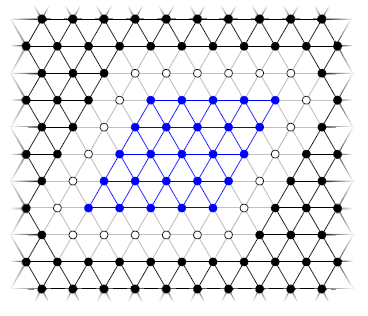
Figure 1. Boundary of a domain in the triangular lattice

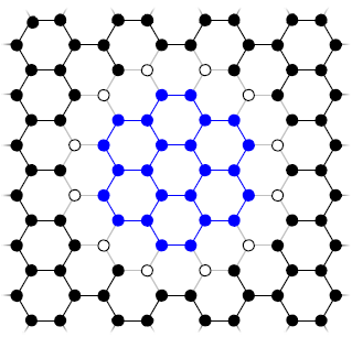
Figure 2. Boundary of a domain in the hexagonal lattice

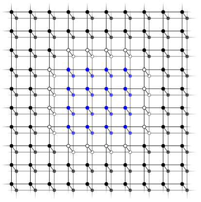
Figure 3. Boundary of a domain in the two dimensional square ladder

Lemma 2.1.

Let $\Sigma=\partial\mathcal{V}_{int}=\partial\mathcal{V}_{ext}$.
(1) $\ \mathcal{V}$ is written as a disjoint union : $\ \mathcal{V}=\stackrel{{\scriptstyle\circ}}{{\mathcal{V}_{int}}}\cup\,\Sigma\,\cup\stackrel{{\scriptstyle\circ}}{{\mathcal{V}_{ext}}}$.
(2)  For any $v\in\Sigma$, $v\sim\stackrel{{\scriptstyle\circ}}{{\mathcal{V}_{int}}}$ and $v\sim\stackrel{{\scriptstyle\circ}}{{\mathcal{V}_{ext}}}$ hold.
(3) Any path starting from $\stackrel{{\scriptstyle\circ}}{{\mathcal{V}_{int}}}$ and ending in $\stackrel{{\scriptstyle\circ}}{{\mathcal{V}_{ext}}}$ passes through $\Sigma$.

Proof. By (B-1-2), $\partial\mathcal{V}_{ext}\subset\mathcal{V}_{ext}$, hence $\mathcal{V}_{ext}=\stackrel{{\scriptstyle\circ}}{{\mathcal{V}_{ext}}}\cup\,\partial\mathcal{V}_{ext}$. Similarly, $\mathcal{V}_{int}=\stackrel{{\scriptstyle\circ}}{{\mathcal{V}_{int}}}\cup\,\partial\mathcal{V}_{int}$. This and (B-1-1) imply (1). Since $\Sigma=\partial\mathcal{V}_{int}=\partial\mathcal{V}_{ext}$, (2) follows. Suppose there exist $v_{i}\in\stackrel{{\scriptstyle\circ}}{{\mathcal{V}_{int}}}$, and $v_{e}\in\stackrel{{\scriptstyle\circ}}{{\mathcal{V}_{ext}}}$ such that $v_{i}\sim v_{e}$. Then $v_{e}\in\partial{\mathcal{V}_{int}}$. This is in contradiction to (1). ∎

The Hilbert space $\ell^{2}(\mathcal{V})$ then admits an orthogonal decomposition

$$\ell^{2}(\mathcal{V})=\ell^{2}(\stackrel{{\scriptstyle\circ}}{{\mathcal{V}_{ext})}}\oplus\,\ell^{2}({\mathcal{V}_{int}}).$$

Let $\widehat{P}_{ext}$ be the associated orthogonal projection :

(2.27) $$\widehat{P}_{ext}:\ell^{2}(\mathcal{V})\to\ell^{2}(\stackrel{{\scriptstyle\circ}}{{\mathcal{V}_{ext}}}).$$

Let ${\widehat{\Delta}}_{\Gamma}$ be the Laplacian on the graph $\Gamma$. We assume that the perturbation $\widehat{V}$ has the following property.

(B-4)  $\widehat{V}$ is bounded self-adjoint on $\ell^{2}(\mathcal{V})$ and has support in $\stackrel{{\scriptstyle\circ}}{{\mathcal{V}_{int}}}$, i.e. $\widehat{V}\widehat{u}=0$ on $\mathcal{V}_{ext}$, $\forall\widehat{u}\in\ell^{2}(\mathcal{V})$.

In [4], the exterior domain $\mathcal{V}_{ext}$ was defined in a slightly different, more restricted form. However, all the arguments there work well for the above $\mathcal{V}_{ext}$ under the above assumptions (B-1) $\sim$ (B-4).

2.4. Function spaces

In [4], for the periodic graph $\Gamma_{0}=\{\mathcal{L}_{0},\mathcal{V}_{0},\mathcal{E}_{0}\}$, the spaces $\ell^{2},\ell^{2,\sigma},\widehat{\mathcal{B}}$, $\widehat{\mathcal{B}}^{\ast}$, $\widehat{\mathcal{B}}^{\ast}_{0}$ were defined as the spaces equipped with the following norms :

(2.28) $$\|\widehat{f}\|^{2}_{\ell^{2}(\mathcal{V}_{0})}=\sum_{n\in\mathcal{V}_{0}}|\widehat{f}(n)|^{2},$$

where (see (2.14))

(2.29) $$|\widehat{f}(n)|^{2}=\sum_{j=1}^{s}|\widehat{f}_{j}(n)|^{2}{\rm deg}_{0}(j),$$

(2.30) $$\|\widehat{f}\|^{2}_{\ell^{2,\sigma}(\mathcal{V}_{0})}=\sum_{n\in\mathcal{V}_{0}}(1+|n|^{2})^{\sigma}|\widehat{f}(n)|^{2},\quad\sigma\in{\bf R},$$

(2.31) $$\|\widehat{f}\|_{\widehat{B}(\mathcal{V}_{0})}^{2}=\sum_{j=0}^{\infty}r_{j}^{1/2}\Big{(}\sum_{r_{j-1}\leq|n|<r_{j},n\in\mathcal{V}_{0}}|\widehat{f}(n)|^{2}\Big{)}^{1/2},$$

where $r_{-1}=0,r_{j}=2^{j}\ (j\geq 0)$,

(2.32) $$\|\widehat{f}\|_{\widehat{\mathcal{B}}^{\ast}(\mathcal{V}_{0})}^{2}=\sup_{R>1}\frac{1}{R}\sum_{|n|<R,n\in\mathcal{V}_{0}}|\widehat{f}(n)|^{2},$$

(2.33) $$\widehat{\mathcal{B}}^{\ast}_{0}(\mathcal{V}_{0})\ni\widehat{f}\Longleftrightarrow\lim_{R\to\infty}\frac{1}{R}\sum_{|n|<R,n\in\mathcal{V}_{0}}|\widehat{f}(n)|^{2}=0.$$

For the perturbed graph $\Gamma$, these spaces are defined as above, replacing $\mathcal{V}_{0}$ by $\stackrel{{\scriptstyle\circ}}{{\mathcal{V}_{ext}}}$ and adding the norm of $\ell^{2}(\mathcal{V}_{int})$. They are denoted by $\ell^{2}(\mathcal{V})$, etc, or sometimes $\ell^{2}$ without fear of confusion.

2.5. Continuous spectrum and embedded eigenvalues

We now define the perturbed Hamiltonian $\widehat{H}$ by

(2.34) $$\widehat{H}=-\widehat{\Delta}_{\Gamma}+\widehat{V}.$$

Let us review the spectral properties of $\widehat{H}$.

Lemma 2.2.

(Theorem 7.1, Lemma 7.2 in [4]).
(1)  $\sigma_{e}(\widehat{H})=\sigma(\widehat{H}_{0})$.
(2) The eigenvalues of $\widehat{H}$ in $\sigma_{e}(\widehat{H})\setminus\mathcal{T}_{1}$ is finite with finite multiplicities.
(3) There is no eigenvalue in $\sigma_{e}(\widehat{H})\setminus\mathcal{T}_{1}$, provided $\widehat{H}$ has the unique continuation property in $\mathcal{V}_{int}$.

The assertions (2) and (3) of Lemma 2.2 are based on the following Rellich type theorem:

Theorem 2.3.

(Theorem 5.1 in [4]). Assume (A-1) and $\lambda\in\sigma_{e}(\widehat{H})\setminus\mathcal{T}_{1}$. If $\widehat{u}\in\widehat{\mathcal{B}}^{\ast}_{0}(\mathcal{V}_{0})$ satisfies

$$(\widehat{H}_{0}-\lambda)\widehat{u}(n)=0,\quad|n|>R_{0},$$

for some $R_{0}>0$, then there exists $R>R_{0}$ such that $\widehat{u}(n)=0$ for $|n|>R$.

Theorem 2.3, for which the assumption (A-1) is essential, plays also an important role in the inverse scattering procedure to be developed in §4. Note, however, by the well-known perturbation theory for the continuous spectrum by Agmon, Kato-Kuroda (see [1], [36]), one can prove the discreteness of embedded eigenvalues, for which we can avoid (A-1), and construct the spectral representation and S-matrix outside the embedded eigenvalues. This was already done in §7 of [4]. In this paper, we always assume (A-1).

2.6. Radiation condition

The well-known radiation condition of Sommerfeld is extended to the discrete Schrödinger operator in the following way.

For $u\in\mathcal{S}^{\prime}({\bf R}^{d})$, the wave front set $WF^{\ast}(u)$ is defined as follows. For $(x_{0},\omega)\in{\bf R}^{d}\times S^{d-1}$, $(x_{0},\omega)\not\in WF^{\ast}(u)$, if there exist $0<\delta<1$ and $\chi\in C_{0}^{\infty}({\bf R}^{d})$ such that $\chi(x_{0})=1$ and

(2.35) $$\lim_{R\to\infty}\frac{1}{R}\int_{|\xi|<R}|C_{\omega,\delta}(\xi)(\widetilde{\chi u})(\xi)|^{2}d\xi=0,$$

where $C_{\omega,\delta}(\xi)$ is the characteristic function of the cone $\{\xi\in{\bf R}^{d}\,;\,\omega\cdot\xi>\delta|\xi|\}$.

We consider distributions on the torus ${\bf T}^{d}={\bf R}^{d}/(2\pi{\bf Z})^{d}$. By using the Fourier series, the counter parts of the spaces $\ell^{2}(\mathcal{V}_{0})$, $\ell^{2,\sigma}(\mathcal{V}_{0}),\widehat{\mathcal{B}}(\mathcal{V}_{0}),\widehat{\mathcal{B}}^{\ast}(\mathcal{V}_{0})$ and $\widehat{\mathcal{B}}^{\ast}_{0}(\mathcal{V}_{0})$ are naturally defined on ${\bf T}^{d}$, which are denoted by $L^{2}({\bf T}^{d}),H^{\sigma}({\bf T}^{d}),\mathcal{B}({\bf T}^{d}),\mathcal{B}^{\ast}({\bf T}^{d})$ and $\mathcal{B}^{\ast}_{0}({\bf T}^{d})$, respectively. As above, we often omit ${\bf T}^{d}$.

Let $H_{0}(x)$ be the matrix in (2.20), and $\lambda_{j}(x),j=1,\cdots,s$, be its eigenvalues. By (A-2) and (A-3), if $\lambda\in\sigma_{e}(\widehat{H})\setminus\mathcal{T}_{0}$, they are simple, and non-characteristic, i.e. $\nabla_{x}\lambda_{j}(x)\neq 0$ on $M_{\lambda,j}$. Let $P_{j}(x)$ be the eigenprojection associated with $\lambda_{j}(x)$. Then, in a small neighborhood of $M_{\lambda,j}$, $P_{j}(x)$ is smooth with respect to $x$. Suppose $u\in\mathcal{B}^{\ast}$ satisfies the equation

(2.36) $$(H_{0}(x)-\lambda)u=f\in\mathcal{B},\quad{\rm on}\quad{\bf T}^{d}.$$

Then, outside $M_{\lambda}$, $u$ is in $\mathcal{B}$. Therefore, when we talk about $WF^{\ast}(u)$, we have only to localize it in a small neighborhood of $M_{\lambda}$. Now, the solution $u$ of the equation (2.36) is said to satisfy the outgoing radiation condition if

(2.37) $$WF^{\ast}(P_{j}u)\subset\{(x,\omega_{x})\,;\,x\in M_{\lambda,j}\},\quad 1\leq j\leq s,$$

where $\omega_{x}$ is the unit normal of $M_{\lambda,j}$ at $x$ such that $\omega_{x}\cdot\nabla\lambda_{j}(x)<0$. Strictly speaking, one must multiply a cut-off function near $M_{\lambda,j}$ to $u$, which is omitted for the sake of simplicity. Similarly, $u$ is said to satisfy the incoming radiation condition, if

(2.38) $$WF^{\ast}(P_{j}u)\subset\{(x,-\omega_{x})\,;\,x\in M_{\lambda,j}\},\quad 1\leq j\leq s.$$

We return to the equation on the perturbed lattice

(2.39) $$(\widehat{H}-\lambda)\widehat{u}=\widehat{f}\quad{\rm on}\quad\mathcal{V}.$$

We say that $\widehat{u}$ satisfies the outgoing (incoming) radiation condition if $\mathcal{U}\widehat{P}_{ext}\widehat{u}$ is outgoing (incoming), where $\mathcal{U}$ and $\widehat{P}_{ext}$ are defined by (1.9) and (2.27).

Let $\widehat{R}(z)=(\widehat{H}-z)^{-1}$, and put

(2.40) $$\mathcal{T}=\mathcal{T}_{0}\cup\mathcal{T}_{1}\cup\mathcal{\sigma}_{p}(\widehat{H}).$$

Lemma 2.4.

(Lemma 7.6 in [4]). If $\lambda\in\sigma_{e}(\widehat{H})\setminus\mathcal{T}$, the solution of the equation (2.39) satisfying the outgoing or incoming radiation condition is unique.

Theorem 2.5.

(Theorem 7.7 in [4]). Take any compact set $I\subset\sigma_{e}(\widehat{H})\setminus\mathcal{T}$, and $\lambda\in I$. Then for any $\widehat{f},\widehat{g}\in\widehat{\mathcal{B}}$, there exists a limit

$$\lim_{\epsilon\to 0}(\widehat{R}(\lambda\pm i0)\widehat{f},\widehat{g})=(\widehat{R}(\lambda\pm i0)\widehat{f},\widehat{g}).$$

Moreover, there exists a constant $C>0$ such that

$$\|\widehat{R}(\lambda\pm i0)\widehat{f}\|_{\widehat{\mathcal{B}}^{\ast}}\leq C\|\widehat{f}\|_{\widehat{\mathcal{B}}},\quad\lambda\in I.$$

For $\widehat{f}\in\widehat{\mathcal{B}}$, $\widehat{R}(\lambda+i0)\widehat{f}$ satisfies the outgoing radiation condition, and $\widehat{R}(\lambda-i0)\widehat{f}$ satisfies the incoming radiation condition. Moreover, letting

(2.41) $$\widehat{Q}_{1}(z)=(\widehat{H}_{0}-z)\widehat{P}_{ext}\widehat{R}(z),$$

(2.42) $$Q_{1}(\lambda\pm i0)=\mathcal{U}_{\mathcal{L}_{0}}\widehat{Q}_{1}(\lambda\pm i0),$$

and $u_{\pm}=\mathcal{U}_{\mathcal{L}_{0}}\widehat{P}_{ext}\widehat{R}(\lambda\pm i0)\widehat{f}$, we have

(2.43) $$P_{j}u_{\pm}\mp\frac{1}{\lambda_{j}(x)-\lambda\mp i0}\otimes\left(P_{j}Q_{1}(\lambda\pm i0)\widehat{f}\right)\Big{|}_{M_{\lambda,j}}\in\mathcal{B}^{\ast}_{0}.$$

2.7. Spectral representation

For the case of $\widehat{H}_{0}$, the spectral representation means the diagonalization of the matrix $H_{0}(x)$. We first prepare its representation space. Take an eigenvector $a_{j}(x)\in{\bf C}^{s}$ of $H_{0}(x)$ satisfying $H_{0}(x)a_{j}(x)=\lambda_{j}(x)a_{j}(x)$, $|a_{j}(x)|=1$. Let ${\bf h}_{\lambda,j}$ be the Hilbert space of ${\bf C}$-valued functions on $M_{\lambda,j}$ equipped with the inner product

$$(\phi,\psi)=\int_{M_{\lambda,j}}\phi(x)\overline{\psi(x)}\frac{dM_{\lambda,j}}{|\nabla\lambda_{j}(x)|}.$$

Put

(2.44) $$I_{j}=\{\lambda_{j}(x)\,;\,x\in{\bf T}^{d}\}\setminus\mathcal{T},$$

(2.45) $$I={\mathop{\cup}_{j=1}^{s}}I_{j}=\sigma(H_{0})\setminus\mathcal{T},$$

(2.46) $${\bf H}_{j}=L^{2}(I_{j},{\bf h}_{\lambda,j}a_{j},d\lambda).$$

We define ${\bf h}_{\lambda,j}$ and ${\bf H}_{j}$ to be $\{0\}$ for $\lambda\in I\setminus I_{j}$, and put

(2.47) $${\bf h}_{\lambda}={\bf h}_{\lambda,1}a_{1}\oplus\cdots\oplus{\bf h}_{\lambda,s}a_{s},$$

(2.48) $${\bf H}={\bf H}_{1}\oplus\cdots\oplus{\bf H}_{s}=L^{2}(I,{\bf h}_{\lambda},d\lambda).$$

For $f\in\mathcal{B}({\bf T}^{d})$, we put

(2.49) $$\mathcal{F}_{0,j}(\lambda)f=\left\{\begin{split}&P_{j}(x)f(x)\Big{|}_{M_{\lambda,j}},\quad{\rm if}\quad\lambda\in I_{j},\\ &0,\quad{\rm otherwise},\end{split}\right.$$

(2.50) $$\mathcal{F}_{0}(\lambda)f=(\mathcal{F}_{0,1}(\lambda)f,\cdots,\mathcal{F}_{0,s}(\lambda)f).$$

(2.51) $$\widehat{\mathcal{F}}_{0}(\lambda)=\mathcal{F}_{0}(\lambda)\mathcal{U}_{\mathcal{L}_{0}}.$$

For the perturbed lattice, we define

(2.52) $$\widehat{\mathcal{F}}^{(\pm)}(\lambda)=\widehat{\mathcal{F}}_{0}(\lambda)\widehat{Q}_{1}(\lambda\pm i0).$$

Note that this is denoted by $\widehat{\mathcal{F}}_{\pm}(\lambda)$ in [4]. Then for any compact set $J\subset\sigma_{e}(\widehat{H})\setminus{\mathcal{T}}$, there exists a constant $C>0$ such that

(2.53) $$\|\widehat{\mathcal{F}}^{(\pm)}(\lambda)\widehat{f}\|_{{\bf h}_{\lambda}}\leq C\|\widehat{f}\|_{\widehat{\mathcal{B}}},\quad\lambda\in J.$$

We define

(2.54) $$\big{(}\widehat{\mathcal{F}}^{(\pm)}\widehat{f}\big{)}(\lambda)=\widehat{\mathcal{F}}^{(\pm)}(\lambda)\widehat{f}.$$

Similarly,

(2.55) $$\big{(}\widehat{\mathcal{F}}_{0}\widehat{f}\big{)}(\lambda)=\widehat{\mathcal{F}}_{0}(\lambda)\widehat{f},\quad\big{(}{\mathcal{F}}_{0}f\big{)}(\lambda)={\mathcal{F}}_{0}(\lambda)f.$$

Let $\widehat{E}(\cdot)$ be the resolution of the identity for $\widehat{H}$.

Theorem 2.6.

(Theorem 7.11 in [4]).
(1) $\ \widehat{\mathcal{F}}^{(\pm)}$ is uniquely extended to a partial isometry with initial set $\mathcal{H}_{ac}(\widehat{H})=\widehat{E}(I)\ell^{2}(\mathcal{V})$ and final set $\bf H$.
(2) $\ \big{(}\widehat{\mathcal{F}}^{(\pm)}\widehat{H}\widehat{f}\big{)}(\lambda)=\lambda\big{(}\widehat{\mathcal{F}}^{(\pm)}\widehat{f}\big{)}(\lambda),\quad\lambda\in\sigma_{e}(\widehat{H})\setminus{\mathcal{T}},\quad\widehat{f}\in\ell^{2}(\mathcal{V})$.
(3)  For $\lambda\in\sigma_{e}(\widehat{H})\setminus{\mathcal{T}}$, $\widehat{\mathcal{F}}^{(\pm)}(\lambda)^{\ast}\in{\bf B}({\bf h}_{\lambda}\,;\,\widehat{\mathcal{B}}^{\ast})$, and $\big{(}\widehat{H}-\lambda\big{)}\widehat{\mathcal{F}}^{(\pm)}(\lambda)^{\ast}\phi=0$ for $\phi\in{\bf h}_{\lambda}$.

The following theorem shows that the spectral representation $\widehat{\mathcal{F}}^{(\pm)}(\lambda)$ appears in the singularity expansion of the resolvent $\widehat{R}(\lambda\pm i0)$. Let

(2.56) $$\widehat{\mathcal{F}}^{(\pm)}(\lambda)\widehat{f}=\left(\widehat{\mathcal{F}}^{(\pm)}_{1}(\lambda)\widehat{f},\cdots,\widehat{\mathcal{F}}^{(\pm)}_{s}(\lambda)\widehat{f}\right).$$

Theorem 2.7.

(Theorem 7.7 in [4]). For $\widehat{f}\in\widehat{\mathcal{B}}$, we have

$$\mathcal{U}_{\mathcal{L}_{0}}\widehat{R}(\lambda\pm i0)\widehat{f}\mp\sum_{j=1}^{s}\frac{1}{\lambda_{j}(x)-\lambda\mp i0}\otimes\widehat{\mathcal{F}}^{(\pm)}_{j}(\lambda)\widehat{f}\in\mathcal{B}^{\ast}_{0}.$$

Note that by (2.42), (2.49) and (2.52),

(2.57) $$\widehat{\mathcal{F}}_{j}^{(\pm)}(\lambda)\widehat{f}=P_{j}Q_{1}(\lambda\pm i0)\widehat{f}\Big{|}_{\Gamma_{\lambda,j}}.$$

2.8. S-matrix

The wave operators are defined by the following strong limit

(2.58) $$\widehat{W}_{\pm}={\mathop{\rm s-lim}_{t\to\pm\infty}}\,e^{it\widehat{H}}\widehat{P}_{ext}e^{-it\widehat{H}_{0}}\widehat{P}_{ac}(\widehat{H}_{0}),$$

where $\widehat{P}_{ac}(\widehat{H}_{0})$ is the projection onto the absolutely continuous subspace for $\widehat{H}_{0}$. The scattering operator is then defined by

(2.59) $$\widehat{S}=\big{(}\widehat{W}_{+}\big{)}^{\ast}\widehat{W}_{-},$$

which is unitary on $\ell^{2}(\mathcal{V}_{0})$. We consider its Fourier transform $S=\widehat{\mathcal{F}}_{0}\widehat{S}\big{(}\widehat{\mathcal{F}}_{0}\big{)}^{\ast}$. Letting

(2.60) $$\widehat{K}_{2}=\widehat{H}\widehat{P}_{ext}-\widehat{P}_{ext}\widehat{H}_{0},$$

(2.61) $$A(\lambda)=\widehat{\mathcal{F}}^{(+)}(\lambda)\widehat{K}_{2}\widehat{\mathcal{F}}_{0}(\lambda)^{\ast}=\widehat{\mathcal{F}}_{0}(\lambda)\widehat{Q}_{1}(\lambda+i0)\widehat{K}_{2}\widehat{F}_{0}(\lambda)^{\ast},$$

we define the S-matrix by

(2.62) $$S(\lambda)=1-2\pi iA(\lambda).$$

Theorem 2.8.

(Theorem 7.13 in [4]) $S(\lambda)$ is unitary on ${\bf h}_{\lambda}$ and

(2.63) $$\left(Sf\right)(\lambda)=S(\lambda)f(\lambda),\quad f\in{\bf H}.$$

This S-matrix appears in the singularity expansion of solutions to the Helmholtz equation in the following way. Define the operator $A_{\pm}(\lambda):{\bf h}_{\lambda}\to\mathcal{B}^{\ast}$ by

(2.64) $$A_{\pm}(\lambda)=\frac{1}{2\pi i}\sum_{j=1}^{s}\frac{1}{\lambda_{j}(x)-\lambda\mp i0}\otimes P_{j}(x)\Big{|}_{x\in M_{\lambda,j}}.$$

Theorem 2.9.

(Theorem 7.15 in [4])
(1) $\ \{\widehat{u}\in\widehat{\mathcal{B}}^{\ast}\,;\,(\widehat{H}-\lambda)\widehat{u}=0\}=\widehat{\mathcal{F}}^{(-)}(\lambda)^{\ast}{\bf h}_{\lambda}$.
(2) For any $\phi^{in}\in{\bf h}_{\lambda}$, there exist unique $\phi^{out}\in{\bf h}_{\lambda}$ and $\widehat{u}\in\widehat{\mathcal{B}}^{\ast}$ satisfying

(2.65) $$\big{(}\widehat{H}-\lambda\big{)}\widehat{u}=0,$$

(2.66) $$\mathcal{U}_{\mathcal{L}_{0}}\widehat{P}_{ext}\widehat{u}+A_{-}(\lambda)\phi^{in}-A_{+}(\lambda)\phi^{out}\in\mathcal{B}_{0}^{\ast}.$$

Moreover,

(2.67) $$S(\lambda)\phi^{in}=\phi^{out}.$$

3. Exterior problem

3.1. Laplacian in the exterior domain

In this section, we study the exterior Dirichlet problem

(3.1) $$\left\{\begin{split}&(-\widehat{\Delta}_{\Gamma_{0}}-z)\widehat{u}=\widehat{f}\quad{\rm in}\quad\stackrel{{\scriptstyle\circ}}{{\mathcal{V}_{ext}}},\\ &\widehat{u}=0\quad{\rm on}\quad\partial\mathcal{V}_{ext}.\end{split}\right.$$

In the exterior domain ${\mathcal{V}_{ext}}$, the spaces $\ell^{2}({\mathcal{V}_{ext}})$, $\ell^{2,\sigma}({\mathcal{V}_{ext}})$, $\widehat{\mathcal{B}}({\mathcal{V}_{ext}})$, $\widehat{\mathcal{B}}^{\ast}({\mathcal{V}_{ext}})$, $\widehat{\mathcal{B}}^{\ast}_{0}({\mathcal{V}_{ext}})$ are defined in the same way as in the case of periodic lattice $\Gamma_{0}=\{\mathcal{L}_{0},\mathcal{V}_{0},\mathcal{E}_{0}\}$. Let $D$ be a connected subset of ${\mathcal{V}_{ext}}$. Then for any function $\widehat{u}=(\widehat{u}_{1},\cdots,\widehat{u}_{s})$ on $D$, its normal derivative at the boundary of $D$ defined by (2.7) is rewritten as

(3.2) $$\big{(}\partial_{\nu}^{D}\widehat{u}\big{)}_{i}(n)=-\frac{1}{{\rm deg}_{D}(i,n)}\sum_{(j,n^{\prime})\in\stackrel{{\scriptstyle\circ}}{{D}},(j,n^{\prime})\sim(i,n)}\widehat{u}_{j}(n^{\prime}),\quad(i,n)\in\partial D,$$

where

(3.3) $${\rm deg}_{D}(i,n)=\left\{\begin{split}&\sharp\{(j,n^{\prime})\,;\,(j,n^{\prime})\in D,\ (j,n^{\prime})\sim(i,n)\},\quad(i,n)\in\,\stackrel{{\scriptstyle\circ}}{{D}},\\ &\sharp\{(j,n^{\prime})\,;\,(j,n^{\prime})\in\,\stackrel{{\scriptstyle\circ}}{{D}},\ (j,n^{\prime})\sim(i,n)\},\quad(i,n)\in\partial D.\end{split}\right.$$

By (2.7) and (2.8), the following Green’s formula holds

(3.4) $$\big{(}\widehat{\Delta}_{\Gamma_{0}}\widehat{u},\widehat{v}\big{)}_{\ell^{2}(\stackrel{{\scriptstyle\circ}}{{D}})}-\big{(}\widehat{u},\widehat{\Delta}_{\Gamma_{0}}\widehat{v}\big{)}_{\ell^{2}(\stackrel{{\scriptstyle\circ}}{{D}})}=\left(\partial_{\nu}^{D}\widehat{u},\widehat{v}\right)_{\ell^{2}(\partial D)}-\left(\widehat{u},\partial_{\nu}^{D}\widehat{v}\right)_{\ell^{2}(\partial D)}.$$

In particular, this holds for $D=\mathcal{V}_{ext}$.

We define a subspace of $\ell^{2}(\mathcal{V}_{ext})$ by

(3.5) $$\ell^{2}_{0}(\mathcal{V}_{ext})=\{\widehat{f}\in\ell^{2}(\mathcal{V}_{ext})\,;\,\ \widehat{f}=0\ {\rm on}\ \partial\mathcal{V}_{ext}\},$$

and let $\widehat{P}_{0,ext}$ be the associated orthogonal projection

(3.6) $$\widehat{P}_{0,ext}\,:\;\ell^{2}(\mathcal{V}_{ext})\to\ell^{2}_{0}(\mathcal{V}_{ext}).$$

Note that $\ell^{2}_{0}(\mathcal{V}_{ext})$ is naturally isomorphic to $\ell^{2}(\stackrel{{\scriptstyle\circ}}{{\mathcal{V}_{ext}}})$. By (3.4), $-\widehat{P}_{0,ext}\widehat{\Delta}_{\Gamma}\widehat{P}_{0,ext}$ is self-adjoint on $\ell^{2}(\mathcal{V}_{ext})$. Here, we extend any function $\widehat{f}\in\ell^{2}(\mathcal{V}_{ext})$ to be 0 outside $\mathcal{V}_{ext}$ so that $\widehat{\Delta}_{\Gamma}$ can be applied to $\widehat{f}$. We take $\ell^{2}_{0}(\mathcal{V}_{ext})$ as the total Hilbert space and define

(3.7) $$\widehat{H}_{ext}=-\widehat{P}_{0,ext}\widehat{\Delta}_{\Gamma_{0}}\widehat{P}_{0,ext}\Big{|}_{\ell^{2}_{0}(\mathcal{V}_{ext})},$$

which is self-adjoint on $\ell^{2}_{0}(\mathcal{V}_{ext})$. Note that

(3.8) $$\widehat{H}_{ext}\widehat{u}=-\widehat{\Delta}_{\Gamma_{0}}\widehat{u}\quad{\rm on}\quad\stackrel{{\scriptstyle\circ}}{{\mathcal{V}_{ext}}},\quad\forall\widehat{u}\in\ell^{2}_{0}(\mathcal{V}_{ext}).$$

In fact, by definition, for $\widehat{u}\in\ell^{2}_{0}(\mathcal{V}_{ext})$

$$\widehat{H}_{ext}\widehat{u}=-\widehat{P}_{0,ext}\widehat{\Delta}_{\Gamma_{0}}\widehat{P}_{0,ext}\widehat{u}=-\widehat{\Delta}_{\Gamma_{0}}\widehat{u}+(1-\widehat{P}_{0,ext})\widehat{\Delta}_{\Gamma_{0}}\widehat{u},$$

and the 2nd term of the right-hand side vanishes on $\stackrel{{\scriptstyle\circ}}{{\mathcal{V}_{ext}}}$.

Lemma 3.1.

(1) $\ \sigma(\widehat{H}_{ext})=\sigma(\widehat{H}_{0})=\sigma_{e}(\widehat{H})=\sigma_{e}(\widehat{H}_{ext})$.
(2) $\ \sigma_{p}(\widehat{H}_{ext})\cap\big{(}\sigma(\widehat{H}_{ext})\setminus(\mathcal{T}_{0}\cup\mathcal{T}_{1})\big{)}=\emptyset$.

Proof. The assertion (1) is proven by the standard method of singular sequences. The assertion (2) follows from Theorem 2.3 and the assumption (B-2). ∎

We show that Lemma 2.4 also holds for the exterior Dirichlet problem. The radiation condition is naturally extended to solutions $\widehat{u}\in\widehat{\mathcal{B}}^{\ast}({\mathcal{V}_{ext}})$ of the equation

(3.9) $$(-\widehat{\Delta}_{\Gamma_{0}}-\lambda)\widehat{u}=0\quad{\rm on}\quad\stackrel{{\scriptstyle\circ}}{{\mathcal{V}_{ext}}}$$

by extending to be 0 outside $\mathcal{V}_{ext}$.

Lemma 3.2.

Let $\lambda\in\sigma_{e}(\widehat{H}_{ext})\setminus\big{(}\mathcal{T}_{0}\cup\mathcal{T}_{1}\big{)}$. If $\widehat{u}\in\widehat{\mathcal{B}}^{\ast}({\mathcal{V}_{ext}})$ satisfies the equation (3.9), the boundary condition $\widehat{u}=0$ on $\partial{\mathcal{V}_{ext}}$ and the radiation condition, then $\widehat{u}$ vanishes identically on $\mathcal{V}_{ext}$.

Proof. We consider the case that $\widehat{u}$ satisfies the outgoing radiation condition. Take $R$ large enough, and split $\widehat{u}$ as $\widehat{u}=\widehat{u}_{e}+\widehat{u}_{0}$, where

$$\widehat{u}_{e}=\left\{\begin{split}&\widehat{u},\quad\forall(j,n)\ {\rm s.t.}\ |n|>R,\\ &0,\quad{\rm otherwise}.\end{split}\right.$$

We first show

(3.10) $${\rm Im}\big{(}(-\widehat{\Delta}_{\Gamma_{0}}-\lambda)\widehat{u}_{e},\widehat{u}_{e})=0.$$

In fact, since $(-\widehat{\Delta}_{\Gamma_{0}}-\lambda)\widehat{u}=0$ holds on $\stackrel{{\scriptstyle\circ}}{{\mathcal{V}_{ext}}}$, we have by using Green’s formula and the fact that $\widehat{u}$, $\widehat{u}_{e}$ and $\widehat{u}_{0}$ vanish on $\partial{\mathcal{V}}_{ext}$

(3.11) $$\begin{split}\big{(}(-\widehat{\Delta}_{\Gamma_{0}}-\lambda)\widehat{u}_{e},\widehat{u}_{e}\big{)}&=\big{(}(-\widehat{\Delta}_{\Gamma_{0}}-\lambda)(\widehat{u}-\widehat{u}_{0}),\widehat{u}_{e}\big{)}=-\big{(}(-\widehat{\Delta}_{\Gamma_{0}}-\lambda)\widehat{u}_{0},\widehat{u}_{e}\big{)}\\ &=-\big{(}\widehat{u}_{0},(-\widehat{\Delta}_{\Gamma_{0}}-\lambda)\widehat{u}_{e}\big{)}=-\big{(}\widehat{u}_{0},(-\widehat{\Delta}_{\Gamma_{0}}-\lambda)(\widehat{u}-\widehat{u}_{0})\big{)}\\ &=\big{(}\widehat{u}_{0},(\widehat{H}_{ext}-\lambda)\widehat{u}_{0}\big{)}.\end{split}$$

The imaginary part of the right-hand side vanishes, since $\widehat{H}_{ext}$ is self-adjoint, and $\widehat{u}_{0}\in D(\widehat{H}_{ext})$.

We now define $\widehat{v}\in\ell^{2}(\mathcal{V}_{0})$ by the 0-extension of $\widehat{u}_{e}$ on whole $\mathcal{V}_{0}$. Then, we have

(3.12) $$(-\widehat{\Delta}_{\Gamma_{0}}-\lambda)\widehat{v}=\widehat{f},$$

where $\widehat{f}$ is compactly supported. Passing to the Fourier series, $v=\mathcal{U}_{\mathcal{L}_{0}}\widehat{v}$ satisfies

(3.13) $$(H_{0}(x)-\lambda)v=f\quad{\rm on}\quad{\bf T}^{d},$$

where $f(x)$ is a trigonometric polynomial. Since $v$ is outgoing, by Lemma 6.2 of [4], we have

$$P_{j}(x)v(x)=\frac{P_{j}(x)f(x)}{\lambda_{j}(x)-\lambda-i0},$$

and also

(3.14) $${\rm Im}\,\big{(}v,f)=\pi\|f\big{|}_{M_{\lambda}}\|^{2}_{L^{2}(M_{\lambda})},$$

which vanishes by virtue of (3.10). Take $x^{(0)}\in M_{\lambda}$ and $\chi(x)\in C^{\infty}({\bf T}^{d})$ such that $\chi(x^{(0)})=1$ and $\chi(x)=0$ outside a small neighborhood of $x^{(0)}$. We multiply the equation $(H_{0}(x)-\lambda)v(x)=f(x)$ by the cofactor matrix of $H_{0}(x)-\lambda$, and also $\chi(x)$. Letting $w(x)=\chi(x)v(x)$, $g(x)=\chi(x)^{co}(H_{0}(x)-\lambda)f(x)$, we have

$$p(x,\lambda)w(x)=g(x),\quad p(x,\lambda)=\det(H_{0}(x)-\lambda).$$

Since $p(x,\lambda)$ is simple characteristic on $M_{\lambda}$, we can make a change of variables $x\to y$ taking $y_{1}=p(x,\lambda)$. We write $w(x(y))$, $g(x(y))$ as $w(y)$, $g(y)$ for the sake of simplicity. Since $w(y)$ is outgoing, by Lemma 6.2 of [4], it is written as

$$w(y)=\frac{g(y)}{y_{1}-i0}.$$

Passing to the Fourier transform, we then have

(3.15) $$\big{\|}\widetilde{w}(\xi_{1},\cdot)-i\theta(-\xi_{1})\int_{-\infty}^{\infty}\widetilde{g}(\eta_{1},\cdot)d\eta_{1}\big{\|}_{L^{2}({\bf R}^{d-1})}\to 0,\quad{\rm as}\quad|\xi_{1}|\to\infty,$$

where $\theta$ is the Heaviside function (see the proof of [4], Lemma 4.5). By virtue of (3.14), $g\big{|}_{M_{\lambda}}=0$ holds. Therefore $g(0,y^{\prime})=0$, hence $\int_{-\infty}^{\infty}\widetilde{g}(\eta_{1},\eta^{\prime})d\eta_{1}=0$. We have by (3.15), $\|\widetilde{w}(\xi_{1},\cdot)\|_{L^{2}({\bf R}^{d-1})}\to 0$ as $\xi_{1}\to\pm\infty$. Therefore, $w(x)$ is both outgoing and incoming, hence $w(x)\in\mathcal{B}_{0}^{\ast}$.

We have thus seen that $\widehat{u}$ is a $\widehat{\mathcal{B}}_{0}^{\ast}$-solution to the $(-\widehat{\Delta}_{\Gamma_{0}}-\lambda)\widehat{u}=0$, hence vanishes identically on $\mathcal{V}_{ext}$ by virtue of Theorem 2.3. ∎

Once we have proven Lemma 3.2, the following Theorem 3.3 can be derived in the same way as in the whole space [4], as was done in Theorem 6.3 of [35] for the square lattice. We do not repeat the details.

We put

(3.16) $$\widehat{R}_{ext}(z)=(\widehat{H}_{ext}-z)^{-1}.$$

(3.17) $$\mathcal{T}_{e}=\mathcal{T}_{0}\cup\mathcal{T}_{1}.$$

Theorem 3.3.

Take any compact set $I\subset\sigma_{e}(\widehat{H}_{ext})\setminus{\mathcal{T}}_{e}$, and $\lambda\in I$. Then for any $\widehat{f},\widehat{g}\in\mathcal{B}^{\ast}$, there exists a limit

(3.18) $$\lim_{\epsilon\to 0}(\widehat{R}_{ext}(\lambda\pm i0)\widehat{f},\widehat{g}):=(\widehat{R}_{ext}(\lambda\pm i0)\widehat{f},\widehat{g}).$$

Moreover, there exists a constant $C>0$ such that

(3.19) $$\|\widehat{R}_{ext}(\lambda\pm i0)\widehat{f}\|_{{\mathcal{B}}^{\ast}}\leq C\|\widehat{f}\|_{\mathcal{B}},\quad\forall\lambda\in I.$$

3.2. Exterior and interior D-N maps

Take $\lambda\in\sigma_{e}(\widehat{H}_{ext})\setminus\mathcal{T}_{e}$, and consider the solution $\widehat{u}^{(\pm)}_{ext}\in\widehat{\mathcal{B}}^{\ast}$ of the following equation

(3.20) $$\left\{\begin{split}(-\widehat{\Delta}_{\Gamma_{0}}-\lambda)\widehat{u}^{(\pm)}_{ext}=0\quad{\rm in}\quad\stackrel{{\scriptstyle\circ}}{{\mathcal{V}_{ext}}},\\ \widehat{u}^{(\pm)}_{ext}=\widehat{f}\quad{\rm on}\quad\partial\mathcal{V}_{ext},\end{split}\right.$$

satisfying the radiation condition (outgoing for $u^{(+)}_{ext}$ and incoming for $u^{(-)}_{ext}$).

Lemma 3.4.

For any $\lambda\in\sigma_{e}(\widehat{H}_{ext})\setminus\mathcal{T}_{e}$, there exists a unique solution $\widehat{u}^{(\pm)}_{ext}$ of the exterior Dirichlet problem (3.20) satisfying the radiation condition.

Proof. The uniqueness follows from Lemma 3.2. To prove the existence, we extend $\widehat{f}$ to be 0 outside $\partial\mathcal{V}_{ext}$ and put

(3.21) $$\widehat{u}^{(\pm)}_{ext}=\widehat{f}-\widehat{P}_{0}\widehat{R}_{ext}(\lambda\pm i0)(-\widehat{\Delta}_{\Gamma_{0}}-\lambda)\widehat{f},$$

where $\widehat{P}_{0}=\widehat{P}_{0,ext}$. Then $\widehat{u}^{(\pm)}_{ext}=\widehat{f}$ on $\partial\mathcal{V}_{ext}$. Letting $\widehat{w}^{(\pm)}=\widehat{P}_{0}\widehat{R}_{ext}(\lambda\pm i0)(-\widehat{\Delta}_{\Gamma_{0}}-\lambda)\widehat{f}$, we have

$$-\widehat{\Delta}_{\Gamma_{0}}\widehat{P}_{0}\widehat{w}^{(\pm)}=-\widehat{P}_{0}\widehat{\Delta}_{\Gamma_{0}}\widehat{P}_{0}\widehat{w}^{(\pm)}=\widehat{H}_{ext}\widehat{w}^{(\pm)}\quad{\rm in}\quad\stackrel{{\scriptstyle\circ}}{{\mathcal{V}_{ext}}}.$$

Here, we note that

$$\begin{split}\widehat{H}_{ext}\widehat{w}^{(\pm)}&=\widehat{H}_{ext}\widehat{R}_{ext}(\lambda\pm i0)(-\widehat{\Delta}_{\Gamma_{0}}-\lambda)\widehat{f}\\ &=(-\widehat{\Delta}_{\Gamma_{0}}-\lambda)\widehat{f}+\lambda\widehat{R}_{ext}(\lambda\pm i0)(-\widehat{\Delta}_{\Gamma_{0}}-\lambda)\widehat{f}.\end{split}$$

Hence

(3.22) $$\begin{split}(-\widehat{\Delta}_{\Gamma_{0}}-\lambda)\widehat{u}^{(\pm)}_{ext}&=(-\widehat{\Delta}_{\Gamma_{0}}-\lambda)\widehat{f}-(\widehat{H}_{ext}-\lambda)\widehat{w}^{(\pm)}\\ &=(1-\widehat{P}_{0})(-\widehat{\Delta}_{\Gamma_{0}}-\lambda)\widehat{f}=0,\quad{\rm in}\quad\stackrel{{\scriptstyle\circ}}{{\mathcal{V}_{ext}}},\end{split}$$

which proves the lemma. ∎

We define the exterior D-N map $\Lambda^{(\pm)}_{ext}(\lambda)$ by

(3.23) $$\Lambda^{(\pm)}_{ext}(\lambda)\widehat{f}=-\partial_{\nu}^{\mathcal{V}_{ext}}\widehat{u}^{(\pm)}_{ext}\Big{|}_{\partial{\mathcal{V}}_{ext}}.$$

By the assumption (B-1-3), $\mathcal{V}_{int}$ is a connected subgraph of $\mathcal{V}$, hence has the Laplacian, which is denoted by $\widehat{\Delta}_{int}$. We define a subspace of $\ell^{2}(\mathcal{V}_{int})$ by

(3.24) $$\ell^{2}_{0}({\mathcal{V}}_{int})=\{\widehat{f}\in\ell^{2}(\mathcal{V}_{int})\,;\,\widehat{f}=0,\ {\rm on}\ \partial{\mathcal{V}}_{int}\},$$

and let $\widehat{P}_{0,int}$ be the associated orthogonal projection

(3.25) $$\widehat{P}_{0,int}:\ell^{2}(\mathcal{V}_{int})\to\ell^{2}_{0}(\mathcal{V}_{int}).$$

We define the interior Schrödinger operator

(3.26) $$\widehat{H}_{int}=-\widehat{P}_{0,int}\widehat{\Delta}_{int}\widehat{P}_{0,int}+\widehat{V},$$

on $\mathcal{V}_{int}$ with Dirichlet boundary condition on $\partial\mathcal{V}_{int}$. Note that by the assumption (B-4), we have

(3.27) $$\widehat{V}=\widehat{P}_{0,int}\widehat{V}\widehat{P}_{0,int}\quad{\rm on}\quad\mathcal{V}_{int}.$$

$\widehat{H}_{int}$ is a finite dimensional operator, hence has a finite discrete spectrum. Then the interior D-N map $\Lambda_{int}(\lambda)$ is defined by

(3.28) $$\Lambda_{int}(\lambda)\widehat{f}=\partial_{\nu}^{\mathcal{V}_{int}}\widehat{u}_{int}\Big{|}_{\partial{\mathcal{V}}_{int}},$$

where $\lambda\not\in\sigma(\widehat{H}_{int})$, and $\widehat{u}_{int}$ is a unique solution to the equation

(3.29) $$\left\{\begin{split}(-\widehat{\Delta}_{int}+\widehat{V}-\lambda)\widehat{u}_{int}=0\quad{\rm in}\quad\stackrel{{\scriptstyle\circ}}{{\mathcal{V}_{int}}},\\ \widehat{u}_{int}=\widehat{f}\quad{\rm on}\quad\partial{\mathcal{V}}_{int}.\end{split}\right.$$

Note that the uniqueness of $\widehat{u}_{int}$ follows from $\lambda\not\in\sigma(\widehat{H}_{int})$ and the existence is shown by putting

$$\widehat{u}_{int}=\widehat{f}-\widehat{P}_{0,int}\widehat{R}_{int}(\lambda)(-\widehat{\Delta}_{int}-\lambda)\widehat{f},$$

where $\widehat{f}$ is extended to be 0 outside $\partial\mathcal{V}_{int}$, and $\widehat{R}_{int}(\lambda)=(\widehat{H}_{int}-\lambda)^{-1}$.

As in Lemma 2.1, we put

$$\Sigma=\partial\mathcal{V}_{int}=\partial\mathcal{V}_{ext},$$

and define an operator $\widehat{S}_{\Sigma}\in{\bf B}(\ell^{2}(\Sigma);\ell^{2}(\mathcal{V}))$ by

(3.30) $$\big{(}\widehat{S}_{\Sigma}\widehat{f}\big{)}(a)=\frac{1}{{\rm deg}_{\mathcal{V}}(a)}\sum_{b\sim a,b\in\Sigma}\widehat{f}(b),$$

where

$${\rm deg}_{\mathcal{V}}(a)={\rm deg}\,(a)=\sharp\{c\in\mathcal{V}\,;\,c\sim a\}$$

is the degree on $\mathcal{V}$. For a subset $A$ in $\mathcal{V}$, let $\chi_{A}$ be the characteristic function of $A$. In the following, we use $\chi_{\Sigma}$ to mean both of the operator of restriction

$$\chi_{\Sigma}:\ell^{2}_{loc}(\mathcal{V})\ni\widehat{f}\to\widehat{f}\Big{|}_{\Sigma},$$

$\ell^{2}_{loc}(\mathcal{V})$ being the set of locally bounded sequences, and the operator of extension

$$\chi_{\Sigma}:\ell^{2}(\Sigma)\ni\widehat{f}\to\left\{\begin{split}&\widehat{f},\quad{\rm on}\quad\Sigma,\\ &0,\quad{\rm otherwise},\end{split}\right.$$

without fear of confusion. Then, we have for $\widehat{f}\in\ell^{2}(\Sigma)$

(3.31) $$\widehat{\Delta}_{\Gamma}\chi_{\Sigma}\widehat{f}=\widehat{S}_{\Sigma}\widehat{f}.$$

We also introduce multiplication operators by

(3.32) $$\big{(}\mathcal{M}_{int}\widehat{f}\big{)}(a)=\frac{{\rm deg}_{\mathcal{V}_{int}}(a)}{{\rm deg}_{\mathcal{V}}(a)}\widehat{f}(a),$$

(3.33) $$\big{(}\mathcal{M}_{ext}\widehat{f}\big{)}(a)=\frac{{\rm deg}_{\mathcal{V}_{ext}}(a)}{{\rm deg}_{\mathcal{V}}(a)}\widehat{f}(a).$$

Lemma 3.5.

Let $\widehat{u}^{(\pm)}_{ext}$ and $\widehat{u}_{int}$ be the solutions of (3.20) and (3.29), and put

(3.34) $$\widehat{u}^{(\pm)}=\chi_{\stackrel{{\scriptstyle\circ}}{{\mathcal{V}_{int}}}}\widehat{u}_{int}+\chi_{\stackrel{{\scriptstyle\circ}}{{\mathcal{V}_{ext}}}}\widehat{u}^{(\pm)}_{ext}+\chi_{\Sigma}\widehat{f}.$$

Then we have

(3.35) $$\widehat{u}^{(\pm)}=\widehat{R}(\lambda\pm i0)\chi_{\Sigma}B^{(\pm)}_{\Sigma}(\lambda)\widehat{f},$$

where

(3.36) $$B^{(\pm)}_{\Sigma}(\lambda)=\mathcal{M}_{int}\Lambda_{int}(\lambda)-\mathcal{M}_{ext}\Lambda^{(\pm)}_{ext}(\lambda)-\widehat{S}_{\Sigma}-\lambda\chi_{\Sigma}.$$

In particular,

(3.37) $$\widehat{u}^{(\pm)}_{ext}=\widehat{R}(\lambda\pm i0)\chi_{\Sigma}B^{(\pm)}_{\Sigma}(\lambda)\widehat{f}\quad{\rm on}\quad\stackrel{{\scriptstyle\circ}}{{\mathcal{V}_{ext}}},$$

(3.38) $$\widehat{f}=\widehat{R}(\lambda\pm i0)\chi_{\Sigma}B^{(\pm)}_{\Sigma}(\lambda)\widehat{f}\quad{\rm on}\quad\Sigma.$$

Proof. Since $\widehat{u}^{(\pm)}=\widehat{u}_{int}$ in $\mathcal{V}_{int}$, and $\widehat{u}^{(\pm)}=\widehat{u}_{ext}^{(\pm)}$ in $\mathcal{V}_{ext}$, we have

(3.39) $$(-\widehat{\Delta}_{\Gamma}+\widehat{V}-\lambda)\widehat{u}^{(\pm)}=0\quad{\rm in}\quad\stackrel{{\scriptstyle\circ}}{{\mathcal{V}_{int}}}\cup\stackrel{{\scriptstyle\circ}}{{\mathcal{V}_{ext}}}.$$

For $a\in\Sigma$, we have

$$\big{(}\widehat{\Delta}_{\Gamma}\,\chi_{\stackrel{{\scriptstyle\circ}}{{\mathcal{V}_{int}}}}\widehat{u}_{int}\big{)}(a)=-\big{(}\mathcal{M}_{int}\partial_{\nu}^{\mathcal{V}_{int}}\widehat{u}_{int}\big{)}(a)=-\big{(}\mathcal{M}_{int}\Lambda_{int}(\lambda)\widehat{f}\big{)}(a),$$

$$\big{(}\widehat{\Delta}_{\Gamma}\,\chi_{\stackrel{{\scriptstyle\circ}}{{\mathcal{V}_{ext}}}}\widehat{u}_{ext}^{(\pm)}\big{)}(a)=-\big{(}\mathcal{M}_{ext}\partial_{\nu}^{\mathcal{V}_{ext}}\widehat{u}_{ext}^{(\pm)}\big{)}(a)=\big{(}\mathcal{M}_{ext}\Lambda_{ext}^{(\pm)}(\lambda)\widehat{f}\big{)}(a).$$

Therefore, we have in view of (3.39)

(3.40) $$\begin{split}&\big{(}-\widehat{\Delta}_{\Gamma}+\widehat{V}-\lambda\big{)}\big{(}\chi_{\stackrel{{\scriptstyle\circ}}{{\mathcal{V}_{int}}}}\widehat{u}_{int}+\chi_{\stackrel{{\scriptstyle\circ}}{{\mathcal{V}_{ext}}}}\widehat{u}_{ext}^{(\pm)}+\chi_{\Sigma}\widehat{f}\big{)}\\ &=\chi_{\Sigma}\left(\mathcal{M}_{int}\Lambda_{int}(\lambda)-\mathcal{M}_{ext}\Lambda_{ext}^{(\pm)}(\lambda)-\big{(}\widehat{\Delta}_{\Gamma}+\lambda)\chi_{\Sigma}\right)\widehat{f}\\ &=\chi_{\Sigma}B^{(\pm)}_{\Sigma}(\lambda)\widehat{f}.\end{split}$$

Taking account of the radiation condition, we get (3.35). ∎

Lemma 3.6.

For any $\lambda\in\sigma_{e}(\widehat{H}_{ext})\setminus\left(\mathcal{T}_{e}\cup\sigma(\widehat{H}_{int})\right)$, and $\widehat{f},\widehat{g}\in\ell^{2}(\Sigma)$, we have

(3.41) $$\big{(}\Lambda_{int}(\lambda)\widehat{f},\widehat{g}\big{)}_{\ell^{2}(\Sigma)}=\big{(}\widehat{f},\Lambda_{int}(\lambda)\widehat{g}\big{)}_{\ell^{2}(\Sigma)},$$

(3.42) $$\big{(}\Lambda_{ext}^{(\pm)}(\lambda)\widehat{f},\widehat{g}\big{)}_{\ell^{2}(\Sigma)}=\big{(}\widehat{f},\Lambda_{ext}^{(\mp)}(\lambda)\widehat{g}\big{)}_{\ell^{2}(\Sigma)}.$$

Proof. The first equality (3.41) follows from Green’s formula (2.8). To show (3.42), let for $z\not\in{\bf R}$

$$\widehat{u}(z)=\chi_{\Sigma}\widehat{f}-\widehat{R}_{ext}(z)\big{(}\chi_{\stackrel{{\scriptstyle\circ}}{{\mathcal{V}_{ext}}}}(-\widehat{\Delta}_{\Gamma}-z)\chi_{\Sigma}\widehat{f}\big{)}.$$

Then, $\widehat{u}(z)$ is the $\ell^{2}$-solution to the exterior Dirichlet problem:

$$\left\{\begin{split}(-\widehat{\Delta}_{\Gamma_{0}}-z)\widehat{u}=0\quad{\rm in}\quad\stackrel{{\scriptstyle\circ}}{{\mathcal{V}_{ext}}},\\ \widehat{u}=\widehat{f}\quad{\rm on}\quad\partial\mathcal{V}_{ext},\end{split}\right.$$

and $\widehat{u}(\lambda+i0)$ ($\widehat{u}(\lambda-i0)$) satisfies the outgoing (incoming) radiation condition. Similarly, we put

$$\widehat{v}(z)=\chi_{\Sigma}\widehat{g}-\widehat{R}_{ext}(z)\big{(}\chi_{\stackrel{{\scriptstyle\circ}}{{\mathcal{V}_{ext}}}}(-\widehat{\Delta}_{\Gamma}-z)\chi_{\Sigma}\widehat{g}\big{)}.$$

Since $\widehat{u}(z)$, $\widehat{v}(z)\in\ell^{2}$, we have by Green’s formula

$$\begin{split}&\big{(}\widehat{\Delta}_{\Gamma_{0}}\widehat{u}(\lambda+i\epsilon),\widehat{v}(\lambda-i\epsilon)\big{)}_{\ell^{2}(\stackrel{{\scriptstyle\circ}}{{\mathcal{V}_{ext}}})}-\big{(}\widehat{u}(\lambda+i\epsilon),\widehat{\Delta}_{\Gamma_{0}}\widehat{v}(\lambda-i\epsilon)\big{)}_{\ell^{2}(\stackrel{{\scriptstyle\circ}}{{\mathcal{V}_{ext}}})}\\ &=-\big{(}\partial_{\nu}^{\mathcal{V}_{ext}}\widehat{u}(\lambda+i\epsilon),\widehat{v}(\lambda-i\epsilon)\big{)}_{\ell^{2}(\Sigma)}+\big{(}\widehat{u}(\lambda+i\epsilon),\partial_{\nu}^{\mathcal{V}_{ext}}\widehat{v}(\lambda-i\epsilon)\big{)}_{\ell^{2}(\Sigma)}.\end{split}$$

Due to the equation $\widehat{\Delta}_{\Gamma_{0}}\widehat{u}=-z\widehat{u}$, the left-hand side vanishes. Letting $\epsilon\to 0$, we get (3.42). ∎

4. Scattering amplitude and D-N maps

4.1. Imbedding of $\ell^{2}(\Sigma)$ into ${\bf h}_{\lambda}$

Let us derive the resolvent equation for $\widehat{H}_{ext}$.

Lemma 4.1.

(1) For $\widehat{f}\in\widehat{\mathcal{B}}(\mathcal{V}_{0})$,

$$\begin{split}\widehat{R}_{ext}(\lambda\pm i0)\chi_{\stackrel{{\scriptstyle\circ}}{{\mathcal{V}}}_{ext}}\widehat{f}=\left(1-\widehat{R}(\lambda\pm i0)\chi_{\Sigma}B^{(\pm)}_{\Sigma}(\lambda)\chi_{\Sigma}\right)\widehat{R}_{0}(\lambda\pm i0)\widehat{f},\end{split}$$

in $\stackrel{{\scriptstyle\circ}}{{\mathcal{V}}}_{ext}$.
(2) For $\widehat{g}\in\widehat{\mathcal{B}}(\stackrel{{\scriptstyle\circ}}{{\mathcal{V}_{ext}}})$,

$$\begin{split}\widehat{R}_{ext}(\lambda\pm i0)\widehat{g}=\widehat{R}_{0}(\lambda\pm i0)\left(1-\chi_{\Sigma}\big{(}B^{(\mp)}_{\Sigma}(\lambda)\big{)}^{\ast}\chi_{\Sigma}\widehat{R}(\lambda\pm i0)\right)\chi_{\stackrel{{\scriptstyle\circ}}{{\mathcal{V}_{ext}}}}\widehat{g},\end{split}$$

in $\stackrel{{\scriptstyle\circ}}{{\mathcal{V}_{ext}}}$.

Proof. Let $\widehat{v}_{0}=\widehat{R}(\lambda\pm i0)\chi_{\Sigma}B^{(\pm)}_{\Sigma}(\lambda)\chi_{\Sigma}\widehat{R}_{0}(\lambda\pm i0)\widehat{f}$. We replace $\widehat{f}$ in (3.34) by $\chi_{\Sigma}\widehat{R}_{0}(\lambda\pm i0)\widehat{f}$. Then, by (3.35), we have

(4.1) $$\begin{split}&\chi_{{\stackrel{{\scriptstyle\circ}}{{\mathcal{V}}}_{int}}}\widehat{u}_{int}+\chi_{{\stackrel{{\scriptstyle\circ}}{{\mathcal{V}}}_{ext}}}\widehat{u}_{ext}^{(\pm)}+\chi_{\Sigma}\widehat{R}_{0}(\lambda\pm i0)\widehat{f}\\ &=\widehat{R}(\lambda\pm i0)\chi_{\Sigma}B^{(\pm)}_{\Sigma}(\lambda)\chi_{\Sigma}\widehat{R}_{0}(\lambda\pm i0)\widehat{f}=\widehat{v}_{0}.\end{split}$$

This implies $\widehat{v}_{0}=\widehat{u}^{(\pm)}_{ext}$ in $\stackrel{{\scriptstyle\circ}}{{\mathcal{V}_{ext}}}$, hence

(4.2) $$\left\{\begin{split}&(-\widehat{\Delta}_{\Gamma_{0}}-\lambda)\widehat{v}_{0}=0\quad{\rm in}\quad{\stackrel{{\scriptstyle\circ}}{{\mathcal{V}_{ext}}}},\\ &\widehat{v}_{0}=\widehat{R}_{0}(\lambda\pm i0)\widehat{f}\quad{\rm on}\quad\Sigma=\partial{\mathcal{V}}_{ext}.\end{split}\right.$$

Let $\widehat{w}=\widehat{v}_{0}-\widehat{R}_{0}(\lambda\pm i0)\widehat{f}$. Then

$$\left\{\begin{split}&(-\widehat{\Delta}_{\Gamma_{0}}-\lambda)\widehat{w}=-\widehat{f}\quad{\rm in}\quad\stackrel{{\scriptstyle\circ}}{{\mathcal{V}_{ext}}},\\ &\widehat{w}=0\quad{\rm on}\quad\partial{\mathcal{V}_{ext}}.\end{split}\right.$$

Taking account of the radiation condition, we then have $\widehat{w}=-\widehat{R}_{ext}(\lambda\pm i0)\chi_{\stackrel{{\scriptstyle\circ}}{{\mathcal{V}_{ext}}}}\widehat{f}=\widehat{v}_{0}-\widehat{R}_{0}(\lambda\pm i0)\widehat{f}$, which implies (1). Taking the adjoint, we obtain (2). ∎

We introduce a spectral representation for $\widehat{H}_{ext}$ by

(4.3) $$\widehat{\mathcal{F}}^{(\pm)}_{ext}(\lambda)=\widehat{\mathcal{F}}_{0}(\lambda)\left(1-\chi_{\Sigma}\big{(}B^{(\mp)}_{\Sigma}(\lambda)\big{)}^{\ast}\chi_{\Sigma}\widehat{R}(\lambda\pm i0)\right)\chi_{\stackrel{{\scriptstyle\circ}}{{\mathcal{V}_{ext}}}}.$$

Lemma 4.1 (2) implies

$$\widehat{\mathcal{F}}^{(\pm)}_{ext}(\lambda)=\widehat{\mathcal{F}}_{0}(\lambda)(\widehat{H}_{0}-\lambda)\widehat{R}_{ext}(\lambda\pm i0)\chi_{\stackrel{{\scriptstyle\circ}}{{\mathcal{V}_{ext}}}}.$$

Therefore, $\widehat{\mathcal{F}}^{(\pm)}_{ext}(\lambda)$ does not depend on the perturbation $\mathcal{V}_{int}$ and $\widehat{V}$. By (4.3), we have

$$\widehat{\mathcal{F}}^{(-)}_{ext}(\lambda)^{\ast}\phi=\chi_{\stackrel{{\scriptstyle\circ}}{{\mathcal{V}_{ext}}}}\left(1-\widehat{R}(\lambda+i0)\chi_{\Sigma}B^{(+)}_{\Sigma}(\lambda)\chi_{\Sigma}\right)\widehat{\mathcal{F}}_{0}(\lambda)^{\ast}\phi.$$

By (3.38), $\widehat{R}(\lambda+i0)\chi_{\Sigma}B^{(+)}_{\Sigma}(\lambda)\chi_{\Sigma}=1$ on $\Sigma$, hence it is natural to define

$$\widehat{\mathcal{F}}^{(-)}_{ext}(\lambda)^{\ast}\phi=0,\quad{\rm on}\quad\Sigma.$$

Then, we have

(4.4) $$\widehat{\mathcal{F}}^{(-)}_{ext}(\lambda)^{\ast}\phi=\left(1-\widehat{R}(\lambda+i0)\chi_{\Sigma}B^{(+)}_{\Sigma}(\lambda)\chi_{\Sigma}\right)\widehat{\mathcal{F}}_{0}(\lambda)^{\ast}\phi,\quad{\rm in}\quad\mathcal{V}_{ext}.$$

Lemma 4.2.

For any $\phi\in{\bf h}_{\lambda}$, $\widehat{\mathcal{F}}^{(-)}_{ext}(\lambda)^{\ast}\phi$ satisfies the equation

(4.5) $$\left\{\begin{split}&(-\widehat{\Delta}_{\Gamma_{0}}-\lambda)\widehat{\mathcal{F}}^{(-)}_{ext}(\lambda)^{\ast}\phi=0\quad{\rm in}\quad{\stackrel{{\scriptstyle\circ}}{{\mathcal{V}_{ext}}}},\\ &\widehat{\mathcal{F}}^{(-)}_{ext}(\lambda)^{\ast}\phi=0\quad{\rm on}\quad\Sigma,\end{split}\right.$$

and $\widehat{\mathcal{F}}^{(-)}_{ext}(\lambda)^{\ast}\phi-{\mathcal{F}}_{0}(\lambda)^{\ast}\phi$ is outgoing.

Proof. By Lemma 3.5, $\widehat{v}=\widehat{R}(\lambda+i0)\chi_{\Sigma}B^{(+)}_{\Sigma}(\lambda)\chi_{\Sigma}\widehat{\mathcal{F}}_{0}(\lambda)^{\ast}\phi$ satisfies

$$(-\widehat{\Delta}_{\Gamma_{0}}-\lambda)\widehat{v}=0\quad{\rm in}\quad\stackrel{{\scriptstyle\circ}}{{\mathcal{V}_{ext}}},\quad\widehat{v}\big{|}_{\Sigma}=\widehat{\mathcal{F}}_{0}(\lambda)^{\ast}\phi.$$

In view of (4.4), noting that $\widehat{\mathcal{F}}_{0}(\lambda)^{\ast}\phi$ satisfies

$$(-\widehat{\Delta}_{\Gamma_{0}}-\lambda)\widehat{\mathcal{F}}_{0}(\lambda)^{\ast}\phi=0\quad{\rm in}\quad\stackrel{{\scriptstyle\circ}}{{\mathcal{V}_{ext}}},$$

we obtain the lemma. ∎

We put

(4.6) $$\widehat{I}^{(\pm)}(\lambda)=\widehat{\mathcal{F}}^{(\pm)}(\lambda)\chi_{\Sigma}B^{(\pm)}_{\Sigma}(\lambda):\ell^{2}(\Sigma)\to{\bf h}_{\lambda}.$$

By (2.41), (2.51) and (2.52), we have

$$\widehat{I}^{(\pm)}(\lambda)=\mathcal{F}_{0}(\lambda)\mathcal{U}_{\mathcal{L}_{0}}(\widehat{H}_{0}-\lambda)\widehat{P}_{ext}\widehat{R}(\lambda\pm i0)\chi_{\Sigma}B^{(\pm)}_{\Sigma}(\lambda),$$

which yields by virtue of (2.27), (3.34) and (3.35)

(4.7) $$\widehat{I}^{(\pm)}(\lambda)\widehat{f}=\mathcal{F}_{0}(\lambda)\mathcal{U}_{\mathcal{L}_{0}}(\widehat{H}_{0}-\lambda)\widehat{P}_{ext}\widehat{u}^{(\pm)}.$$

This formula shows that $I^{(\pm)}(\lambda)$ depends neither on $\mathcal{V}_{int}$ nor on $\widehat{V}$, i.e. it is independent of the perturbation.

Lemma 4.3.

(1) $\ \widehat{I}^{(\pm)}(\lambda):\ell^{2}(\Sigma)\to{\bf h}_{\lambda}$ is 1 to 1.
(2) $\ \widehat{I}^{(\pm)}(\lambda)^{\ast}:{\bf h}_{\lambda}\to\ell^{2}(\Sigma)$ is onto.

Proof. Suppose $\widehat{I}^{(\pm)}(\lambda)\widehat{f}=0$, and let $\widehat{u}^{(\pm)}_{ext}$ be the solution to (3.20). In view of (3.34) and (3.35), we have in $\stackrel{{\scriptstyle\circ}}{{\mathcal{V}_{ext}}}$,

$$\widehat{u}^{(\pm)}_{ext}=\widehat{R}(\lambda\pm i0)\widehat{g},\quad\widehat{g}=\chi_{\Sigma}B^{(\pm)}_{\Sigma}(\lambda)\widehat{f}.$$

Theorem 2.7 implies

$$\mathcal{U}_{\mathcal{L}_{0}}\widehat{R}(\lambda\pm i0)\widehat{g}\mp\sum_{j=1}^{s}\frac{1}{\lambda_{j}(x)-\lambda\mp i0}\otimes\widehat{\mathcal{F}}_{j}^{(\pm)}(\lambda)\widehat{g}\in{\mathcal{B}}^{\ast}_{0}.$$

Since $\widehat{I}^{(\pm)}(\lambda)\widehat{f}=\widehat{\mathcal{F}}^{(\pm)}(\lambda)\widehat{g}$, this implies $\widehat{u}^{(\pm)}_{ext}\in\widehat{\mathcal{B}}^{\ast}_{0}$. The Rellich type theorem (Theorem 2.3) and the unique continuation property (B-2) entails $\widehat{u}^{(\pm)}_{ext}=0$, which yields $\widehat{f}=0$. This proves (1), which implies that the range of $\widehat{I}^{(\pm)}(\lambda)^{\ast}$ is dense. Since $\ell^{2}(\Sigma)$ is finite dimensional, (2) follows. ∎

4.2. Scattering amplitude in the exterior domain

Similarly to the scattering amplitude (2.61), we define the scattering amplitude in the exterior domain by

(4.8) $$A_{ext}(\lambda)=\widehat{\mathcal{F}}^{(+)}(\lambda)\chi_{\Sigma}B^{(+)}_{\Sigma}(\lambda)\chi_{\Sigma}\widehat{\mathcal{F}}_{0}(\lambda)^{\ast}.$$

Using Theorem 2.7 and (4.4), and extending $\widehat{\mathcal{F}}^{(-)}_{ext}(\lambda)^{\ast}\phi-\widehat{\mathcal{F}}_{0}(\lambda)^{\ast}\phi$ to be 0 outside $\mathcal{V}_{ext}$, we have

(4.9) $$\begin{split}\mathcal{U}_{\mathcal{L}_{0}}\left(\widehat{\mathcal{F}}^{(-)}_{ext}(\lambda)^{\ast}\phi-\widehat{\mathcal{F}}_{0}(\lambda)^{\ast}\phi\right)&=-\mathcal{U}_{\mathcal{L}_{0}}\widehat{R}(\lambda+i0)\chi_{\Sigma}B^{(+)}_{\Sigma}(\lambda)\chi_{\Sigma}\widehat{\mathcal{F}}_{0}(\lambda)^{\ast}\phi\\ &\simeq-\sum_{j=1}^{s}\frac{1}{\lambda_{j}(x)-\lambda-i0}\otimes A_{ext,j}(\lambda)\phi,\end{split}$$

where $A_{ext,j}(\lambda)\phi$ denotes the $j$-th component of $A_{ext}(\lambda)\phi$. This shows that $A_{ext}(\lambda)\phi$ depends only on $\mathcal{V}_{ext}$.

4.3. Single layer and double layer potentials

The operator

(4.10) $$\widehat{R}(\lambda\pm i0)\chi_{\Sigma}B^{(\pm)}_{\Sigma}(\lambda):\ell^{2}(\Sigma)\to\mathcal{B}^{\ast}(\mathcal{V})$$

is an analogue of the double layer potential in the continuous case. Similarly, the operator defined by

(4.11) $$\ell^{2}(\Sigma)\ni\widehat{f}\to M^{(\pm)}_{\Sigma}(\lambda)\widehat{f}:=\left(\widehat{R}(\lambda\pm i0)\chi_{\Sigma}\widehat{f}\right)\Big{|}_{\Sigma}\in\ell^{2}(\Sigma)$$

is an analogue of the single layer potential.

Lemma 4.4.

$M^{(\pm)}_{\Sigma}(\lambda)B^{(\pm)}_{\Sigma}(\lambda)=1$ on $\ell^{2}(\Sigma)$.

This follows from (3.38). In particular, $M^{(\pm)}_{\Sigma}(\lambda)=(B^{(\pm)}_{\Sigma}(\lambda))^{-1}$.

4.4. S-matrix and interior D-N map

The scattering amplitude $A(\lambda)$ in the whole space (2.61) and the scattering amplitude $A_{ext}(\lambda)$ in the exterior domain (4.8) have the following relation.

Theorem 4.5.

We have

(4.12) $$A_{ext}(\lambda)-A(\lambda)=\widehat{I}^{(+)}(\lambda)\left(B^{(+)}_{\Sigma}(\lambda)\right)^{-1}\widehat{I}^{(-)}(\lambda)^{\ast}.$$

Proof. For $\phi\in{\bf h}_{\lambda}$, let

(4.13) $$\widehat{u}=\widehat{\mathcal{F}}^{(-)}(\lambda)^{\ast}\phi-\widehat{\mathcal{F}}^{(-)}_{ext}(\lambda)^{\ast}\phi.$$

By (2.42) and (2.60), we have

$$\begin{split}\widehat{Q}_{1}(\lambda-i0)=(\widehat{H}_{0}-\lambda)\widehat{P}_{ext}\widehat{R}(\lambda-i0)=-\widehat{K}_{2}^{\ast}\widehat{R}(\lambda-i0)+\widehat{P}_{ext}.\end{split}$$

Using (2.52) and (4.4), we then have

(4.14) $$\widehat{u}=\left((\widehat{P}_{ext}-1)+\widehat{R}(\lambda+i0)(\chi_{\Sigma}B_{\Sigma}^{(+)}(\lambda)\chi_{\Sigma}-\widehat{K}_{2})\right)\widehat{\mathcal{F}}_{0}(\lambda)^{\ast}\phi.$$

Theorem 2.7 then implies

(4.15) $$\mathcal{U}_{\mathcal{L}_{0}}\widehat{u}\simeq\sum_{j=1}^{d}\frac{1}{\lambda_{j}(x)-\lambda-i0}\otimes\widehat{\mathcal{F}}^{(+)}_{j}(\lambda)(\chi_{\Sigma}B^{(+)}_{\Sigma}(\lambda)\chi_{\Sigma}-\widehat{K}_{2})\widehat{\mathcal{F}}_{0}(\lambda)^{\ast}\phi.$$

By virtue of Lemma 4.2, $\widehat{u}$ is the outgoing solution of the equation

(4.16) $$(-\widehat{\Delta}_{\Gamma_{0}}-\lambda)\widehat{u}=0\quad{\rm in}\quad\stackrel{{\scriptstyle\circ}}{{\mathcal{V}}}_{ext},\quad\widehat{u}\big{|}_{\Sigma}=\widehat{\mathcal{F}}^{(-)}(\lambda)^{\ast}\phi.$$

Lemma 3.5 yields

(4.17) $$\widehat{u}=\widehat{R}(\lambda+i0)\chi_{\Sigma}B^{(+)}(\lambda)\widehat{\mathcal{F}}^{(-)}(\lambda)^{\ast}\phi.$$

Again using Theorem 2.7,

(4.18) $$\mathcal{U}_{\mathcal{L}_{0}}\widehat{u}\simeq\sum_{j=1}^{d}\frac{1}{\lambda_{j}(x)-\lambda-i0}\otimes\widehat{\mathcal{F}}_{j}^{(+)}(\lambda)\chi_{\Sigma}B_{\Sigma}^{(+)}(\lambda)\widehat{\mathcal{F}}^{(-)}(\lambda)^{\ast}\phi.$$

Comparing (4.15) and (4.18), we have

(4.19) $$\begin{split}&\widehat{\mathcal{F}}^{(+)}(\lambda)(\chi_{\Sigma}B^{(+)}_{\Sigma}(\lambda)\chi_{\Sigma}-\widehat{K}_{2})\widehat{\mathcal{F}}_{0}(\lambda)^{\ast}\phi\\ &=\widehat{\mathcal{F}}^{(+)}(\lambda)\chi_{\Sigma}B_{\Sigma}^{(+)}(\lambda)\widehat{\mathcal{F}}^{(-)}(\lambda)^{\ast}\phi.\end{split}$$

By (2.61) and (4.8), the left-hand side is equal to $A_{ext}(\lambda)-A(\lambda)$.

Let us note here that $1=B^{(-)}_{\Sigma}(\lambda)M^{(-)}_{\Sigma}(\lambda)$ by virtue of Lemma 4.4. Since $M^{(\pm)}_{\Sigma}(\lambda)=\chi_{\Sigma}\widehat{R}(\lambda\pm i0)\chi_{\Sigma}$, we have $(M^{(-)}_{\Sigma}(\lambda))^{\ast}=M^{(+)}_{\Sigma}(\lambda)$, which implies

(4.20) $$1=M^{(+)}_{\Sigma}(\lambda)\big{(}B^{(-)}_{\Sigma}(\lambda)\big{)}^{\ast}.$$

Inserting (4.20) between $B^{(+)}_{\Sigma}(\lambda)$ and $\widehat{\mathcal{F}}^{(-)}(\lambda)^{\ast}\phi$, we obtain

(4.21) $$\begin{split}&\widehat{\mathcal{F}}^{(+)}(\lambda)\chi_{\Sigma}B^{(+)}\chi_{\Sigma}\widehat{\mathcal{F}}^{(-)}(\lambda)^{\ast}\\ &=\widehat{\mathcal{F}}^{(+)}(\lambda)\chi_{\Sigma}B^{(+)}_{\Sigma}(\lambda)M^{(+)}_{\Sigma}(\lambda)\big{(}B^{(-)}_{\Sigma}(\lambda)\big{)}^{\ast}\chi_{\Sigma}\widehat{\mathcal{F}}^{(-)}(\lambda)^{\ast}\\ &=\widehat{I}^{(+)}(\lambda)M^{(+)}_{\Sigma}(\lambda)\widehat{I}^{(-)}(\lambda)^{\ast}.\end{split}$$

We have thus proven (4.12). ∎

4.5. The operator $\widehat{J}^{(\pm)}(\lambda)$

To construct $A(\lambda)$ from $B^{(+)}_{\Sigma}(\lambda)$, we need to invert $\widehat{I}^{(\pm)}(\lambda)$ and its adjoint. To compute them, we first construct a solution $\widehat{u}^{(\pm)}_{ext}$ to the exterior Dirichlet problem satisfying (3.20) and the radiation condition in the form $\widehat{R}_{0}(\lambda\pm i0)\widehat{\psi}$, where $\widehat{\psi}\in\ell^{2}(\Sigma)$. Then it is the desired solution if and only if

(4.22) $$\widehat{R}_{0}(\lambda\pm i0)\widehat{\psi}=\widehat{f}\quad{\rm on}\quad\Sigma.$$

Suppose $\widehat{R}_{0}(\lambda\pm i0)\widehat{\phi}^{(\pm)}=0$ on $\Sigma$. Then, $\widehat{v}^{(\pm)}=\widehat{R}_{0}(\lambda\pm i0)\widehat{\phi}^{(\pm)}$ is the solution to the equation (3.20) with 0 boundary data. Since $\widehat{v}^{(\pm)}$ satisfies the radiation condition, by Lemma 3.2, it vanishes identically in $\stackrel{{\scriptstyle\circ}}{{\mathcal{V}}}_{ext}$ hence on all $\mathcal{V}_{0}$. It then follows that $\widehat{\phi}^{(\pm)}=0$. Therefore, the equation (4.22) is uniquely solvable for any $\widehat{f}\in\ell^{2}(\Sigma)$. Let $\widehat{\psi}=\widehat{r}_{\Sigma}^{(\pm)}(\lambda)\widehat{f}$ be the solution. Then, we have

(4.23) $$\widehat{u}^{(\pm)}_{ext}=\widehat{R}_{0}(\lambda\pm i0)\widehat{r}_{\Sigma}^{(\pm)}(\lambda)\widehat{f},$$

which is a potential theoretic solution to the boundary value problem (3.20).

Let $\widehat{g}_{n},n=1,\cdots,N$, be a basis of $\ell^{2}(\Sigma)$ and put

(4.24) $$\begin{split}v^{(\pm)}_{n}&=\widehat{I}^{(\pm)}(\lambda)\widehat{g}_{n}\\ &=\mathcal{F}_{0}(\lambda)\mathcal{U}_{\mathcal{L}_{0}}(\widehat{H}_{0}-\lambda)\widehat{P}_{ext}\widehat{R}_{0}(\lambda\pm i0)\widehat{r}_{\Sigma}^{(\pm)}(\lambda)\widehat{g}_{n}\in{\bf h}_{\lambda}.\end{split}$$

Let $\mathcal{M}_{\Sigma}^{(\pm)}$ be the linear hull of $v^{(\pm)}_{1},\cdots,v^{(\pm)}_{N}$. Then, the mapping $\widehat{g}_{n}\to v_{n}^{(\pm)}$ induces a bijection

$$\widehat{J}^{(\pm)}(\lambda):\ell^{2}(\Sigma)\ni\sum_{n=1}^{N}c_{n}\widehat{g}_{n}\to\sum_{n=1}^{N}c_{n}v^{(\pm)}_{n}\in\mathcal{M}_{\Sigma}^{(\pm)}.$$

In view of Theorem 4.5, we have the following theorem.

Theorem 4.6.

The following formula holds:

(4.25) $$\big{(}B^{(+)}_{\Sigma}(\lambda)\big{)}^{-1}=\big{(}\widehat{J}^{(+)}(\lambda)\big{)}^{-1}\big{(}A_{ext}(\lambda)-A(\lambda)\big{)}\big{(}\widehat{J}^{(-)}(\lambda)^{\ast}\big{)}^{-1}.$$

By virtue of Theorems 4.5 and 4.6, the S-matrix and the D-N map determine each other.

4.6. Perturbation of S-matrices

Suppose we are given two interior domains ${\mathcal{V}}_{int,1}$ and ${\mathcal{V}}_{int,2}$ such that $\Sigma=\partial{\mathcal{V}}_{int,1}=\partial{\mathcal{V}}_{int,2}$ and

(4.26) $${\rm deg}_{{\mathcal{V}}_{int,1}}={\rm deg}_{{\mathcal{V}}_{int,2}}\quad{\rm on}\quad\Sigma.$$

We put the suffix $i=1,2,$ for the operators $A(\lambda)$, $\Lambda_{int}(\lambda)$, $\mathcal{M}_{int}$, $\widehat{S}_{\Sigma}$ and $B^{(+)}_{\Sigma}(\lambda)$ associated with the domain $\mathcal{V}_{int,i}$. Then, by the condition (4.26),

(4.27) $$\mathcal{M}_{int,1}=\mathcal{M}_{int,2},\quad\widehat{S}_{\Sigma,1}=\widehat{S}_{\Sigma,2}\quad{\rm on}\quad\Sigma.$$

Then, we have by the resolvent equation,

(4.28) $$\begin{split}&(B^{(+)}_{\Sigma,2}(\lambda))^{-1}-(B^{(+)}_{\Sigma,1}(\lambda))^{-1}\\ &=-(B^{(+)}_{\Sigma,2}(\lambda))^{-1}(\mathcal{M}_{int}\Lambda_{int,2}(\lambda)-\mathcal{M}_{int}\Lambda_{int,1}(\lambda))(B^{(+)}_{\Sigma,1}(\lambda))^{-1},\end{split}$$

where $\mathcal{M}_{int}=\mathcal{M}_{int,1}=\mathcal{M}_{int,2}$. Theorem 4.5 then implies the following lemma.

Lemma 4.7.

The following formula holds:

$$\begin{split}&A_{2}(\lambda)-A_{1}(\lambda)\\ &=\widehat{I}^{(+)}(\lambda)\big{(}B^{(+)}_{\Sigma,2}(\lambda)\big{)}^{-1}\mathcal{M}_{int}\big{(}\Lambda_{int,2}(\lambda)-\Lambda_{int,1}(\lambda)\big{)}\big{(}B^{(+)}_{\Sigma,1}(\lambda)\big{)}^{-1}\widehat{I}^{(-)}(\lambda)^{\ast}.\end{split}$$

Therefore, if we can find a data $\widehat{f}$ on $\Sigma$ such that $\big{(}\Lambda_{int,2}(\lambda)-\Lambda_{int,1}(\lambda)\big{)}\widehat{f}\neq 0$, we can distinguish between $\mathcal{V}_{int,1}$ and $\mathcal{V}_{int,2}$ by the scattering experiment.

5. Asymptotic behavior of wave functions in the lattice space

We have defined the S-matrix by using the singularity expansion of the solution to the Schrödinger equation. However, in some energy region, we can derive it from the spatial asymptotics at infinity of the lattice space. We prove it here because of its physical importance, although it is not used in the later sections.

Recall that by (2.61) and (2.62),

(5.1) $$\phi^{out}=S(\lambda)\phi^{in},$$

(5.2) $$\phi^{out}=\phi^{in}-2\pi i\mathcal{F}_{0}(\lambda)\mathcal{U}_{\mathcal{L}_{0}}\widehat{Q}_{1}(\lambda+i0)\widehat{K}_{2}\widehat{\mathcal{F}}_{0}(\lambda)^{\ast}\phi^{in}.$$

We compute $\widehat{Q}_{1}(z)$ as follows

(5.3) $$\begin{split}\widehat{Q}_{1}(z)=(\widehat{H}_{0}-z)\widehat{P}_{ext}\widehat{R}(z)=\widehat{P}_{ext}+\widehat{K}_{1}\widehat{R}(z),\end{split}$$

(5.4) $$\widehat{K}_{1}=\widehat{H}_{0}\widehat{P}_{ext}-\widehat{P}_{ext}\widehat{H}.$$

Since $\widehat{K}_{1}$ and $\widehat{K}_{2}$ are finite dimensional operators, (5.2) implies that $\phi^{out}\in C^{\infty}(M_{\lambda})$ if $\phi^{in}\in C^{\infty}(M_{\lambda})$. By Theorem 2.9, there exists a unique $\widehat{u}\in\widehat{\mathcal{B}}^{\ast}$ satisfying (2.65), (2.66). We observe the behavior of $\widehat{u}$ modulo $\widehat{\mathcal{B}}^{\ast}_{0}$. In view of Theorem 2.9, we have only to study

(5.5) $$\frac{1}{\lambda_{j}(x)-\lambda\mp i0}\otimes\big{(}P_{j}(x)\phi^{(\pm)}(x)\big{)}\Big{|}_{x\in M_{\lambda,j}},$$

where $\phi^{(+)}=\phi^{out},\phi^{(-)}=\phi^{in}$.

Here we impose a new assumption which is used only in this section :

(C) There exists $\lambda\in\sigma_{e}(\widehat{H})\setminus{\mathcal{T}}$ such that for any $1\leq j\leq s$, $M_{\lambda,j}$ is strictly convex.

Note that in the Assumption (C), we allow the case in which $M_{\lambda,j}=\emptyset$ for some $j$. Let us compute the asymptotic expansion of the integral

(5.6) $$I(k)=\int_{{\bf T}^{d}}\frac{e^{ix\cdot k}f(x)}{\lambda(x)-\lambda\mp i0}dx,$$

assuming that $M_{\lambda}=\{x\in{\bf T}^{d}\,;\,\lambda(x)=\lambda\}$ is strictly convex. It is well-known that

(5.7) $$I(k)=\pm i\pi\int_{M_{\lambda}}\frac{e^{ix\cdot k}f(x)}{|\nabla\lambda(x)|}dM_{\lambda}+{\rm p.v}\int_{{\bf T}^{d}}\frac{e^{ix\cdot k}f(x)}{\lambda(x)-\lambda}dx.$$

Let $N(x)$ be the outward unit normal field at $x\in M_{\lambda}$. Since $M_{\lambda}$ is strictly convex, for any $\omega\in S^{d-1}$, there exists a unique $x^{(\pm)}(\lambda,\omega)\in M_{\lambda}$ such that

$$N(x^{(\pm)}(\lambda,\omega))=\pm\omega.$$

Letting $\omega_{k}=k/|k|$, we have by the stationary phase method

$$I(k)=\sum_{\pm}|k|^{-(d-1)/2}e^{ik\cdot x^{(\pm)}(\lambda,\omega_{k})}a^{(\pm)}(\lambda,\omega_{k})f(x^{(\pm)}(\lambda,\omega_{k}))+O(|k|^{-(d+1)/2}),$$

$$a^{(\pm)}(\lambda,\omega_{k})=C_{\pm}\frac{K(x^{(\pm)}(\lambda,\omega_{k}))^{-1/2}}{|\nabla\lambda(x^{(\pm)}(\lambda,\omega_{k}))|}$$

as $|k|\to\infty$, where $C_{\pm}=\pm i(2\pi)^{(d-1)/2}e^{\mp i(d-1)\pi/4}$ and $K(x)$ is the Gaussian curvature of $M_{\lambda}$ at $x\in M_{\lambda}$ (see Lemma 4.4 of [35]). We replace $\lambda(x)$ by $\lambda_{j}(x)$, and define $x_{j}^{(\pm)}(\lambda,\omega)$, $a_{j}^{(\pm)}(\lambda,\omega)$ and $K_{j}(x)$ in the same way as above. We can thus reformulate (2.66) into the the following theorem.

Theorem 5.1.

Assume (C). If $\widehat{u}\in\widehat{B}^{\ast}$ satisfies $(\widehat{H}-\lambda)\widehat{u}=0$ and $\phi^{in},\phi^{out}\in C^{\infty}(M_{\lambda})$, we have the following asymptotic expansion in the lattice space

(5.8) $$\begin{split}\widehat{u}=&-\sum_{j=1}^{s}|k|^{-(d-1)/2}e^{ik\cdot x^{(-)}_{j}(\lambda,\omega_{k})}a_{j}^{(-)}(\lambda,\omega_{k})\phi_{j}^{in}(x^{(-)}_{j}(\lambda,\omega_{k}))\\ &+\sum_{j=1}^{s}|k|^{-(d-1)/2}e^{ik\cdot x^{(+)}_{j}(\lambda,\omega_{k})}a_{j}^{(+)}(\lambda,\omega_{k})\phi_{j}^{out}(x^{(+)}_{j}(\lambda,\omega_{k}))\\ &+O(|k|^{-(d+1)/2}).\end{split}$$

The standard way of defining the S-matrix is to use the asymptotic expansion of the form (5.8), i.e. the operator

(5.9) $$\phi^{in}_{j}(x^{(-)}_{j}(\lambda,\omega_{k}))\to\phi^{out}_{j}(x^{(+)}_{j}(\lambda,\omega_{k})),\quad\omega_{k}\in S^{d-1}$$

is the S-matrix based on the far field pattern of wave functions. This coincides with our definition of S-matrix (2.62) up to the parametrization of $M_{\lambda}$ (i.e. $\omega$ or $x^{(\pm)}(\lambda,\omega)$). We omit the proof of this fact.

Let us check the assumption (C) in our case. For all of the examples given in [4], $p(x,\lambda)=\det(H_{0}(x)-\lambda)$ is written as

$$p(x,\lambda)=f(a_{d}(x),\lambda),\quad{\rm or}\quad f(b_{d}(x),\lambda),$$

where $f(z,\lambda)$ is a polynomial of two variables $z,\lambda$, and

$$a_{d}(x)=\sum_{j=1}^{d}\cos x_{j},\quad b_{d}(x)=\sum_{j=1}^{d}\cos x_{j}+\sum_{1\leq j<k\leq d}\cos(x_{j}-x_{k}).$$

We factorize $p(x,\lambda)$ as:

$$p(x,\lambda)=c_{0}(\lambda)\left\{\begin{split}&\prod_{i=1}^{m}(a_{d}(x)-c_{i}(\lambda))^{\mu_{i}},\quad(A)\\ &\prod_{i=1}^{m}(b_{d}(x)-c_{i}(\lambda))^{\mu_{i}},\quad(B)\end{split}\right.$$

where $c_{i}(\lambda)\neq c_{j}(\lambda)$ if $i\neq j$.

The case (A). In this case, $M_{\lambda,j}=\{x\in{\bf T}^{d}\,;\,\,a_{d}(x)=c_{i}(\lambda)\}$ for some $i$. Let

(5.10) $$I^{\prime}_{d}=\left\{\begin{split}&(-2,0)\cup(0,2),\quad{\rm for}\quad d=2,\\ &(-d,-d+1)\cup(d-1,d),\quad{\rm for}\quad d\geq 3.\end{split}\right.$$

By Lemma 2.1 of [4], we have

(5.11) $$a_{d}({\bf T}^{d})=[-d,d],$$

and by Lemma 4.3 of [35], for $c\in I_{d}^{\prime}$, the surface $\{x\in{\bf T}^{d}\,;\,a_{d}(x)=c\}$ is strictly convex (see Figures 5 and 5).

Figure 4. $a_{3}(x)=c\in I^{\prime}_{3}$

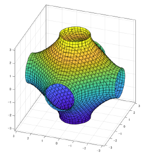
Figure 5. $a_{3}(x)=c\in(-3,3)\setminus I^{\prime}_{3}$

In view of the formulas given in §3 of [4], we thus have:

• For the square lattice,

  $$p(x,\lambda)=-\frac{1}{d}\left(a_{d}(x)+\lambda d\right).$$

  Hence, $M_{\lambda}$ is strictly convex for $\lambda\in(-1,0)\cup(0,1)$ when $d=2$, and for $\lambda\in(-1,-1+1/d)\cup(1-1/d,1)$ when $d\geq 3$.

• For the subdivision of $d$-dim. square lattice,

  $$p(x,\lambda)=-\frac{(-\lambda)^{d-1}}{2d}\left(a_{d}(x)-2d\lambda^{2}+d\right).$$

  Therefore, when $d=2$, $M_{\lambda}$ is strictly convex, if

  $$\lambda\in\big{(}-1,1\big{)}\setminus\Big{\{}\pm\sqrt{\frac{1}{2}},0\Big{\}},$$

  and when $d\geq 3$, if

  $$\lambda\in\Big{(}-1,-\sqrt{1-\frac{1}{2d}}\Big{)}\cup\Big{(}-\sqrt{\frac{1}{2d}},0\Big{)}\cup\Big{(}0,\sqrt{\frac{1}{2d}}\Big{)}\cup\Big{(}\sqrt{1-\frac{1}{2d}},1\Big{)}.$$

• For the ladder of $d$-dim. square lattice,

  $$p(x,\lambda)=\Big{(}\frac{2}{2d+1}\Big{)}^{2}\Big{(}a_{d}(x)+\frac{(2d+1)\lambda+1}{2}\Big{)}\Big{(}a_{d}(x)+\frac{(2d+1)\lambda-1}{2}\Big{)}.$$

  Therefore, when $d=2$, $M_{\lambda}$ is strictly convex if

  $$\lambda\in\big{(}-1,1\big{)}\setminus\big{\{}\pm\frac{1}{5}\big{\}},$$

  and when $d\geq 3$ if

  $$\lambda\in\Big{(}-1,-\frac{2d-3}{2d+1}\Big{)}\cup\Big{(}\frac{2d-3}{2d+1},1\Big{)}\setminus\big{\{}\pm\frac{2d-1}{2d+1}\big{\}}.$$

The case (B). In this case, $M_{\lambda,j}=\{x\in{\bf T}^{d}\,;\,\,b_{d}(x)=c_{i}(\lambda)\}$ for some $i$. For the sake of simplicity, we consider only the case $d=2$. By Lemma 2.2 of [4], we have $b_{2}({\bf T}^{2})=[-3/2,3]$.

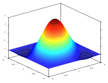
Figure 6. $x_{3}=b_{2}(x_{1},x_{2})$

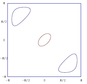
Figure 7. $b_{2}(x_{1},x_{2})=\kappa$

Put $C_{\kappa}=\{x\in{\bf T}^{2}\,;\,b_{2}(x)=\kappa\}$. Taking note of the inequality $\cos x_{1}+\cos x_{2}+\cos(x_{1}-x_{2})\leq 3$, and noting that the equality occurs only when $x_{1}=x_{2}=0$, we have $C_{3}=\{(0,0)\}$. Therefore, if $3-\epsilon<\kappa<3$, $\epsilon>0$ being chosen sufficiently small, $C_{\kappa}$ is a regular closed curve enclosing $(0,0)$. By the Taylor expansion,

$$b_{2}(x_{1},x_{2})=\frac{3}{2}-\frac{1}{2}(x_{1}^{2}-x_{1}x_{2}+x_{2}^{2})+O(|x|^{3}),$$

which does not vanish on $C_{\kappa}$ for $3-\epsilon<\kappa<3$. Therefore, $C_{\kappa}$ is strictly convex if $3-\epsilon<\kappa<3$.

We also have $\cos x_{1}+\cos x_{2}+\cos(x_{1}-x_{2})\geq-3/2$, and the equality occurs only when $(x_{1},x_{2})=(4\pi/3,2\pi/3),(2\pi/3,4\pi/3)$. Therefore,

$$C_{-3/2}=\{(4\pi/3,2\pi/3),(2\pi/3,4\pi/3)\}.$$

Letting $\xi=(x_{1}-4\pi/3,x_{2}-2\pi/3)$ or $(x_{1}-2\pi/3,x_{2}-4\pi/3)$, we have

$$b_{2}(x_{1},x_{2})=-\frac{3}{2}+\frac{1}{2}(x_{1}^{2}-x_{1}x_{2}+x_{2}^{2})+O(|x|^{3}).$$

Therefore, $C_{\kappa}$ is strictly convex if $-3/2<\kappa<-3/2+\epsilon$.

In view of §3 of [4], we obtain :

• For the triangular lattice,

  $$p(x,\lambda)=-\frac{1}{3}\big{(}b_{2}(x)+3\lambda\big{)}.$$

  Therefore, $M_{\lambda}$ is strictly convex for $-1<\lambda<-1+\epsilon$, and $1/2-\epsilon<\lambda<1/2$.

• For the hexagonal lattice,

  $$p(x,\lambda)=-\frac{2}{9}\big{(}b_{2}(x)-\frac{9\lambda^{2}-3}{2}\big{)}.$$

  Therefore, $M_{\lambda}$ is strictly convex for $-1<\lambda<-1+\epsilon$, $\lambda\in(-\epsilon,\epsilon)\setminus\{0\}$, and $1-\epsilon<\lambda<1$.

• For the Kagome lattice,

  $$p(x,\lambda)=\frac{1}{8}\big{(}\lambda-\frac{1}{2}\big{)}\big{(}b_{2}(x)-8\lambda^{2}-4\lambda+1\big{)}.$$

  Therefore, $M_{\lambda}$ is strictly convex for $-1<\lambda<-1+\epsilon$, $\lambda\in(-1/4-\epsilon,-1/4+\epsilon)\setminus\{-1/4\}$ and $1/2-\epsilon<\lambda<1/2$.

• For the graphite,

  $$p(x,\lambda)=\frac{1}{64}\big{(}b_{2}(x)-(8\lambda^{2}+4\lambda-1)\big{)}\big{(}b_{2}(x)-(8\lambda^{2}-4\lambda-1)\big{)}.$$

  Therefore, $M_{\lambda}$ is strictly convex for $-1<\lambda<-1+\epsilon$, $\lambda\in(\pm 1/2-\epsilon,\pm 1/2+\epsilon)\setminus\{\pm 1/2\}$, $(\pm 1/4-\epsilon,\pm 1/4+\epsilon)\setminus\{\pm 1/4\}$ and $1-\epsilon<\lambda<1$.

6. Reconstruction of scalar potentials

6.1. Parallelogram in the hexagonal lattice

In this section, we reconstruct a scalar potential from the D-N map on a bounded domain following the works [14], [17], [51], [35]. This method depends strongly on the geometry of the lattice. Therefore, we explain it for the 2-dimensional hexagonal lattice. First let us recall its structure. We identify ${\bf R}^{2}$ with ${\bf C}$, and put

$$\omega=e^{\pi i/3}.$$

For $n=n_{1}+in_{2}\in{\bf Z}[i]={\bf Z}+i{\bf Z}$, let

$$\mathcal{L}_{0}=\left\{{\bf v}(n)\,;\,n\in{\bf Z}[i]\right\},\quad{\bf v}(n)=n_{1}{\bf v}_{1}+n_{2}{\bf v}_{2},$$

$${\bf v}_{1}=1+\omega=(3+\sqrt{3}i)/2,\quad{\bf v}_{2}=\omega(1+\omega)=\sqrt{3}i,$$

$$p_{1}=\omega^{-1}=\omega^{5},\quad p_{2}=1,$$

and define the vertex set $\mathcal{V}_{0}$ by

$$\mathcal{V}_{0}=\mathcal{V}_{01}\cup\mathcal{V}_{02},\quad\mathcal{V}_{0i}=p_{i}+\mathcal{L}_{0}.$$

The adjacent points of $a_{1}\in\mathcal{V}_{01}$ and $a_{2}\in\mathcal{V}_{02}$ are defined by

$$\begin{split}\mathcal{N}_{a_{1}}&=\{z\in{\bf C}\,;\,|a_{1}-z|=1\}\cap\mathcal{V}_{02}\\ &=\left\{a_{1}+\omega,a_{1}+\omega^{3},a_{1}+\omega^{5}\right\},\end{split}$$

$$\begin{split}\mathcal{N}_{a_{2}}&=\{z\in{\bf C}\,;\,|a_{2}-z|=1\}\cap\mathcal{V}_{01}\\ &=\left\{a_{2}+1,a_{2}+\omega^{2},a_{2}+\omega^{4}\right\}.\end{split}$$

Let $\mathcal{D}_{0}$ be the fundamental domain by the ${\bf Z}^{2}$-action (2.12) on $\mathcal{V}_{0}$. It is a hexagon with 6 vertices $\omega^{k},\ 0\leq k\leq 5$, with center at the origin. Take $D_{N}=\{n\in{\bf Z}[i]\,;\,0\leq n_{1}\leq N,\ 0\leq n_{2}\leq N\}$, where $N$ is chosen large enough, and put

$$\mathcal{D}_{N}={\mathop{\cup}_{n\in D_{N}}}\Big{(}\mathcal{D}_{0}+{\bf v}(n)\Big{)}.$$

This is a parallelogram in the hexagonal lattice.

Figure 8. Hexagonal parallelogram ($N=2$)

The interior angle of each vertex on the periphery of $\mathcal{D}_{N}$ is either $2\pi/3$ or $4\pi/3$. Let $\mathcal{A}$ be the set of the vertices with interior angle $2\pi/3$. We regard $\mathcal{D}_{N}$ to be a subgraph of the original graph $\Gamma_{0}=\{\mathcal{L}_{0},\mathcal{V}_{0},\mathcal{E}_{0}\}$, and for each $z\in\mathcal{A}$, let $e_{z,\zeta}\in\mathcal{E}_{0}$ be the outward edge emanating from $z$, and $\zeta=t(e_{z,\zeta})$ its terminal point. (See Figure 8 for the case $N=2$.) Let $\Omega$ be the set of vertices of the resulting graph. The boundary $\partial\Omega=\{t(e_{z,\zeta})\,;\,z\in\mathcal{A}\}$ is divided into 4 parts, called top, bottom, right, left sides, which are denoted by $(\partial\Omega)_{T},(\partial\Omega)_{B},(\partial\Omega)_{R},(\partial\Omega)_{L}$, i.e.

$$\begin{split}(\partial\Omega)_{T}=&\{\alpha_{0},\cdots,\alpha_{N}\},\\ (\partial\Omega)_{B}=&\{2\omega^{5}+k(1+\omega)\,;\,0\leq k\leq N\},\\ (\partial\Omega)_{R}=&\{2+N(1+\omega)+k\sqrt{3}i\,;\,1\leq k\leq N\}\cup\{2+N(1+\omega)+N\sqrt{3}i+2\omega^{2}\},\\ (\partial\Omega)_{L}=&\{2\omega^{4}\}\cup\{\beta_{0},\cdots,\beta_{N}\},\end{split}$$

where $\alpha_{k}=\beta_{N}+2\omega+k(1+\omega)$ and $\beta_{k}=-2+k\sqrt{3}i$ for $0\leq k\leq N$.

6.2. Matrix representation

Our argument is close to that for the resistor network. To facilitate the comparison, we change the definition of the Laplacian as follows.

(6.1) $$\big{(}\widehat{\Delta}^{\prime}_{\Omega}\widehat{u})(v)=\frac{1}{{\rm deg}_{\Omega}(v)}\sum_{w\sim v}\left(\widehat{u}(v)-\widehat{u}(w)\right)=\widehat{u}(v)-\big{(}\widehat{\Delta}_{\Omega}\widehat{u})(v).$$

Putting

(6.2) $$\widehat{Q}=\widehat{V}-\lambda-1,$$

we consider the Dirichlet problem

(6.3) $$\left\{\begin{split}&\big{(}\widehat{\Delta}^{\prime}_{\Omega}+\widehat{Q}\big{)}\widehat{u}=0\quad{\rm in}\quad\stackrel{{\scriptstyle\circ}}{{\Omega}},\\ &\widehat{u}=\widehat{f}\quad{\rm on}\quad\partial\Omega.\end{split}\right.$$

We assume the unique solvability of this equation. Then, the D-N map is defined by

(6.4) $$\big{(}\Lambda_{\widehat{Q}}\widehat{f}\big{)}(v)=\partial_{\nu}^{\Omega}\widehat{u}(v).$$

Given 4 vertices $z^{(0)}\in\,\stackrel{{\scriptstyle\circ}}{{\Omega}}$, $z^{(0)}+\omega^{k}$, $z^{(0)}+\omega^{k+2}$, $z^{(0)}+\omega^{k+4}\in\Omega$, where $k=0$ or 1, let us call $z^{(0)}$ the central point and $z^{(0)}+\omega^{k+2j}$ the peripheral point. If $\widehat{u}$ satisfies $(\widehat{\Delta}^{\prime}_{\Omega}+\widehat{Q})\widehat{u}=0$, we have

(6.5) $$\widehat{u}(z^{(0)})-\frac{1}{3}\sum_{j=0}^{2}\widehat{u}(z^{(0)}+\omega^{k+2j})+\widehat{Q}(z^{(0)})\widehat{u}(z^{(0)})=0.$$

Therefore, we can compute the value at a peripheral point $\widehat{u}(z^{(0)}+\omega^{k+2\ell})$ using the values at the central point $\widehat{u}(z^{(0)})$, the other peripheral points $\widehat{u}(z^{(0)}+\omega^{k+2j})$, $j\neq\ell$, and $\widehat{Q}(z^{(0)})$. Moreover, if we know the values of $\widehat{u}(z^{(0)})$ and $\widehat{u}(z^{(0)}+\omega^{k+2j})$, we can compute the potential $\widehat{Q}(z^{(0)})$ as long as $\widehat{u}(z^{(0)})\neq 0$.

We split the vertex set of $\Omega$ into two parts:

$${\mathcal{V}}_{0}=\,\stackrel{{\scriptstyle\circ}}{{\Omega}}\,=\{z^{(1)},\cdots,z^{(\nu)}\},\quad\mathcal{V}_{1}=\partial\Omega=\{z^{(\nu+1)},\cdots,z^{(\nu+\mu)}\}.$$

Let us define matrices ${\bf D}=\left(d_{ij}\right)$, ${\bf A}=\left(a_{ij}\right)$ by

$$d_{ij} = \left\{\begin{split}&1,\quad{\rm if}\quad i=j,\\ &0,\quad{\rm if}\quad i\neq j,\end{split}\right.$$

$$a_{ij} = \left\{\begin{split}\big{(}\mathrm{deg}_{\Omega}(z^{(i)})\big{)}^{-1}&,\quad{\rm if}\quad z^{(i)}\sim z^{(j)}\quad{\rm for}\quad z^{(i)}\in\,\stackrel{{\scriptstyle\circ}}{{\Omega}}\quad{\rm or}\quad z^{(j)}\in\,\stackrel{{\scriptstyle\circ}}{{\Omega}},\\ 0&,\quad{\rm if}\quad z^{(i)}\not\sim z^{(j)}\quad{\rm or}\quad z^{(i)},\ z^{(j)}\in\partial\Omega.\end{split}\right.$$

We define a $(\nu+\mu)\times(\nu+\mu)$ matrix ${\bf H}_{0}$ by

$${\bf H}_{0}={\bf D}-{\bf A},$$

which corresponds to (6.1). Since $\widehat{Q}$ is a scalar potential supported in $\stackrel{{\scriptstyle\circ}}{{\Omega}}$, it is identified with the diagonal matrix ${\bf Q}=\left(q_{ij}\right)$, where

$$q_{ij}=\left\{\begin{split}\widehat{Q}(z^{(i)}),&\quad{\rm if}\quad i=j\leq\nu,\\ 0,&\quad{\rm if}\quad i\neq j\quad{\rm or}\quad\ i=j\geq\nu+1.\end{split}\right.$$

We put

(6.6) $${\bf H}={\bf H}_{0}+{\bf Q}.$$

In the following, $\widehat{u}(\mathcal{V}_{i})$ denotes a vector in ${\bf C}^{\sharp\mathcal{V}_{i}}$, and ${\bf H}(\mathcal{V}_{i};\mathcal{V}_{j})$ denotes a $\sharp\mathcal{V}_{i}\times\sharp\mathcal{V}_{j}$-submatrix of ${\bf H}$. For the solution $\widehat{u}$ to the boundary value problem (6.3), noting $\mathrm{deg}_{\Omega}(v)=1$ for $v\in\partial\Omega$, we rewrite the D-N map by

(6.7) $$\big{(}\Lambda_{\widehat{Q}}\widehat{f}\big{)}(v)=\sum_{w\in\stackrel{{\scriptstyle\circ}}{{\Omega}},w\sim v}\big{(}\widehat{f}(v)-\widehat{u}(w)\big{)}=\widehat{f}(v)+\big{(}\partial^{\Omega}_{\nu}\widehat{u}\big{)}(v),\quad v\in\partial\Omega.$$

Then, (6.3) together with (6.7) is rewritten as the following system of equations

(6.8) $$\left(\begin{array}[]{cc}{\bf H}(\mathcal{V}_{0};\mathcal{V}_{0})&{\bf H}(\mathcal{V}_{0};\mathcal{V}_{1})\\ {\bf H}(\mathcal{V}_{1};\mathcal{V}_{0})&{\bf H}(\mathcal{V}_{1};\mathcal{V}_{1})\end{array}\right)\left(\begin{array}[]{c}\widehat{u}(\mathcal{V}_{0})\\ \widehat{f}(\mathcal{V}_{1})\end{array}\right)=\left(\begin{array}[]{c}0\\ \Lambda_{\widehat{Q}}\widehat{f}\end{array}\right).$$

It is easy to see that

(6.9) $$0\not\in\sigma(\widehat{\Delta}^{\prime}_{\Omega}+\widehat{Q})\Longleftrightarrow\det{\bf H}(\mathcal{V}_{0};\mathcal{V}_{0})\neq 0.$$

In fact, assume that 0 is not a Dirichlet eigenvalue of $\widehat{\Delta}^{\prime}_{\Omega}+\widehat{Q}$, and ${\bf H}(\mathcal{V}_{0};\mathcal{V}_{0})\widehat{u}(\mathcal{V}_{0})=0$. Then, letting $\widehat{u}\big{|}_{\partial\Omega}=\widehat{f}=0$, we see that $\widehat{u}$ satisfies (6.3). Since $0\not\in\sigma(\widehat{\Delta}^{\prime}_{\Omega}+\widehat{Q})$, we have $\widehat{u}=0$, which implies $\det{\bf H}(\mathcal{V}_{0};\mathcal{V}_{0})\neq 0$. Conversely, suppose $\widehat{u}$ satisfies (6.3) with $\widehat{f}=0$. Then, (6.8) is satisfied with $\widehat{f}=0$. Hence ${\bf H}(\mathcal{V}_{0};\mathcal{V}_{0})\widehat{u}(\mathcal{V}_{0})=0$ and $\mathrm{det}{\bf H}(\mathcal{V}_{0}:\mathcal{V}_{0})\not=0$ imply $\widehat{u}(\mathcal{V}_{0})=0$. This proves $0\not\in\sigma(\widehat{\Delta}^{\prime}_{\Omega}+\widehat{Q})$.

From now on we assume that

(D)  $0\not\in\sigma(\widehat{\Delta}^{\prime}_{\Omega}+\widehat{Q})$.

Hence the D-N map $\Lambda_{\widehat{Q}}$ has the following matrix representation

(6.10) $${\bf{\Lambda}}_{\bf{\widehat{Q}}}={\bf{H}}(\mathcal{V}_{1};\mathcal{V}_{1})-{\bf H}(\mathcal{V}_{1};\mathcal{V}_{0}){\bf H}(\mathcal{V}_{0};\mathcal{V}_{0})^{-1}{\bf H}(\mathcal{V}_{0};\mathcal{V}_{1}).$$

The key to the inverse procedure is the following partial data problem.

Lemma 6.1.

(1) Given a partial Dirichlet data $\widehat{f}$ on $\partial\Omega\setminus(\partial\Omega)_{R}$, and a partial Neumann data $\widehat{g}$ on $(\partial\Omega)_{L}$, there is a unique solution $\widehat{u}$ on $\stackrel{{\scriptstyle\circ}}{{\Omega}}\cup(\partial\Omega)_{R}$ to the equation

(6.11) $$\left\{\begin{split}&(\widehat{\Delta}^{\prime}_{\Omega}+\widehat{Q})\widehat{u}=0\quad{\rm in}\quad\stackrel{{\scriptstyle\circ}}{{\Omega}},\\ &\widehat{u}=\widehat{f}\quad{\rm on}\quad\partial\Omega\setminus(\partial\Omega)_{R},\\ &\partial_{\nu}^{\Omega}\widehat{u}=\widehat{g}\quad{\rm on}\quad(\partial\Omega)_{L}.\end{split}\right.$$

(2) For subsets $A,B\subset\partial\Omega$, we denote the associated submatrix of $\bf{\Lambda_{\widehat{Q}}}$ by ${\bf\Lambda_{\widehat{\bf Q}}}(A;B)$. Then, the submatrix ${\bf\Lambda_{\widehat{\bf Q}}}((\partial\Omega)_{L};(\partial\Omega)_{R})$ is non-singular, i.e.

$${\bf\Lambda_{\widehat{\bf Q}}}((\partial\Omega)_{L};(\partial\Omega)_{R}):(\partial\Omega)_{R}\to(\partial\Omega)_{L}$$

is a bijection.
(3) Given the D-N map ${\bf\Lambda_{\widehat{\bf Q}}}$, a partial Dirichlet data $\widehat{f}_{2}$ on $\partial\Omega\setminus(\partial\Omega)_{R}$ and a partial Neumann data $\widehat{g}$ on $(\partial\Omega)_{L}$, there exists a unique $\widehat{f}$ on $\partial\Omega$ such that $\widehat{f}=\widehat{f}_{2}$ on $\partial\Omega\setminus(\partial\Omega)_{R}$ and ${\bf\Lambda_{\widehat{\bf Q}}}\widehat{f}=\widehat{g}$ on $(\partial\Omega)_{L}$.

Proof. (1) Look at Figure 8. The values of $\widehat{u}(x_{1}+ix_{2})$ at $\omega^{4}$ and on the line $x_{1}=-1$ are computed from the D-N map and the values of $\widehat{f}$, $\widehat{g}$. Uisng the equation (6.5), one can then compute $\widehat{u}(x_{1}+ix_{2})$ on $\omega^{5}$ and the line $x_{1}=-1/2$. (For the line $x_{1}=-1/2$, start from $\omega^{2}$ and go up). This and the Dirichlet data $\widehat{f}(x_{1}+ix_{2})$ at $2\omega^{5}$ give $\widehat{u}(x_{1}+ix_{2})$ on $1$ and the line $x_{1}=1/2$. Repeating this procedure, we get $\widehat{u}(z)$ for all $z\in\Omega$.

(2) Suppose $\widehat{f}=0$ on $\partial\Omega\setminus(\partial\Omega)_{R}$ and $\Lambda_{\widehat{\bf Q}}\widehat{f}=0$ on $(\partial\Omega)_{L}$. By (1), the solution $\widehat{u}$ vanishes identically. Hence $\widehat{f}=0$ on $(\partial\Omega)_{R}$. This proves the injectivity, hence the surjectivity.

(3) We seek $\widehat{f}$ in the form

$$({\bf{\Lambda_{\widehat{\bf Q}}}}\widehat{f})\big{|}_{(\partial\Omega)_{L}}={\bf{\Lambda_{\widehat{\bf Q}}}}((\partial\Omega)_{L};(\partial\Omega)_{R})\widehat{f}_{1}+{\bf\Lambda_{\widehat{\bf Q}}}((\partial\Omega)_{L};\partial\Omega\setminus(\partial\Omega)_{R})\widehat{f}_{2}=\widehat{g},$$

where $\widehat{f}_{1}=\widehat{f}\big{|}_{(\partial\Omega)_{R}}$. By (2), we have only to take

$$\widehat{f}_{1}=\left({\bf\Lambda_{\widehat{\bf Q}}}((\partial\Omega)_{L};(\partial\Omega)_{R})\right)^{-1}\left(\widehat{g}-{\bf\Lambda_{\widehat{\bf Q}}}((\partial\Omega)_{L};\partial\Omega\setminus(\partial\Omega)_{R})\widehat{f}_{2}\right).\qed$$

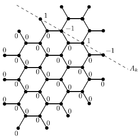
Figure 9. Line $A_{k}$

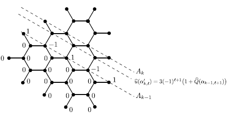
Figure 10. Line $A_{k}^{\prime}$

Now, for $0\leq k\leq N$, let us consider a diagonal line $A_{k}$ :

(6.12) $$A_{k}=\{x_{1}+ix_{2}\,;\,x_{1}+\sqrt{3}x_{2}=a_{k}\},$$

where $a_{k}$ is chosen so that $A_{k}$ passes through

(6.13) $$\alpha_{k}=\alpha_{0}+k(1+\omega)\in(\partial\Omega)_{R}.$$

The vertices on $A_{k}\cap\Omega$ are written as

(6.14) $$\alpha_{k,\ell}=\alpha_{k}+\ell(1+\omega^{5}),\quad\ell=0,1,2,\cdots.$$

We also need another diagonal line $A_{k}^{\prime}$ between $A_{k}$ and $A_{k-1}$ :

(6.15) $$A_{k}^{\prime}=\{x_{1}+ix_{2}\,;\,x_{1}+\sqrt{3}x_{2}=a_{k}^{\prime}\},$$

where $a_{k}^{\prime}$ is such that $A_{k}^{\prime}$ passes through

(6.16) $$\alpha_{k}^{\prime}=\alpha_{k}+\omega^{5}.$$

The vertices on $A_{k}^{\prime}\cap\Omega$ are written as

(6.17) $$\alpha_{k,\ell}^{\prime}=\alpha^{\prime}_{k}+\ell(1+\omega^{5}),\quad\ell=0,1,2,\cdots.$$

Finally, we let

(6.18) $$A_{N+1}^{\prime}=\{x_{1}+ix_{2}\,;\,x_{1}+\sqrt{3}x_{2}=a_{N+1}^{\prime}\},$$

which passes through

(6.19) $$\alpha_{N+1}^{\prime}=\alpha_{N}+2=2+N(1+\omega)+N\sqrt{3}i+2\omega^{2}.$$

Lemma 6.2.

(1) Let $A_{k}\cap\partial\Omega=\{\alpha_{k,0},\alpha_{k,m}\}$. Then there exists a unique solution $\widehat{u}$ to the equation

$$(\widehat{\Delta}^{\prime}_{\Omega}+\widehat{Q})\widehat{u}=0\quad{\rm in}\quad\stackrel{{\scriptstyle\circ}}{{\Omega}},$$

with partial Dirichlet data $\widehat{f}$ such that

(6.20) $$\left\{\begin{split}&\widehat{f}(\alpha_{k,0})=1,\\ &\widehat{f}(\alpha_{k,m})=(-1)^{m},\\ &\widehat{f}(z)=0\quad{\rm for}\quad z\in\partial\Omega\setminus\left((\partial\Omega)_{R}\cup\{\alpha_{k,0}\cup\alpha_{k,m}\}\right),\end{split}\right.$$

and partial Neumann data $\widehat{g}=0$ on $(\partial\Omega)_{L}$. It satisfies

(6.21) $$\widehat{u}(x_{1}+ix_{2})=0\quad{\rm if}\quad x_{1}+\sqrt{3}x_{2}<a_{k},$$

and on $x_{1}+\sqrt{3}x_{2}=a_{k}$,

(6.22) $$\widehat{u}(\alpha_{k,\ell})=(-1)^{\ell},\quad\ell=0,1,2,\cdots.$$

(2) Using the solution $\widehat{u}$ for the data (6.20) with $k$ replaced by $k-1$, $\widehat{Q}(\alpha_{k-1,\ell+1})$ is computed as

(6.23) $$\widehat{Q}(\alpha_{k-1,\ell+1})=\frac{\widehat{u}(\alpha^{\prime}_{k,\ell})}{3(-1)^{\ell+1}}-1,\quad\ell=0,1,2,\cdots.$$

Proof. The uniqueness of $\widehat{u}$ follows from Lemma 6.1. To prove the existence, we argue as in the proof of Lemma 6.1 (1). By the equation (6.5) with central point below $A^{\prime}_{k}$ and the condition on $\widehat{f}$, $\widehat{g}$, one can compute $\widehat{u}(x_{1}+ix_{2})$ successively to obtain (6.21). Using again (6.5), putting central point on $A^{\prime}_{k}$, we obtain (6.22).

We replace $k$ by $k-1$ in the above procedure. Then, $\widehat{u}(z)$ is computed as

$$\widehat{u}(x_{1}+ix_{2})=\left\{\begin{split}0&,\quad{\rm if}\quad x_{1}+\sqrt{3}x_{2}<a_{k-1},\\ (-1)^{\ell}&,\quad{\rm if}\quad x_{1}+ix_{2}=\alpha_{k-1,\ell}.\end{split}\right.$$

We use (6.5) with central point $\alpha_{k-1,\ell+1}\in A_{k-1}$. Then,

$$\big{(}1+\widehat{Q}(\alpha_{k-1,\ell+1})\big{)}\widehat{u}(\alpha_{k-1,\ell+1})=\frac{1}{3}\widehat{u}(\alpha^{\prime}_{k,\ell}),$$

which shows (6.23). ∎

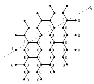
Figure 11. Line $B_{\ell}$

Let us exchange the roles of $(\partial\Omega)_{R}$, $(\partial\Omega)_{L}$ and $(\partial\Omega)_{T}$, $(\partial\Omega)_{B}$. For $0\leq\ell\leq N$, consider a diagonal line $B_{\ell}$

(6.24) $$B_{\ell}=\{x_{i}+ix_{2}\,;\,x_{1}-\sqrt{3}x_{2}=b_{\ell}\},$$

where $b_{\ell}$ is chosen so that $B_{\ell}$ passes through

(6.25) $$\beta_{\ell}=-2+\ell\sqrt{3}i\in(\partial\Omega)_{L}.$$

The vertices on $B_{\ell}\cap\Omega$ are written as

(6.26) $$\beta_{k,\ell}=\beta_{\ell}+k(1+\omega),\quad k=0,1,2,\cdots.$$

Another diagonal line is

(6.27) $$B^{\prime}_{\ell}=\{x_{i}+ix_{2}\,;\,x_{1}-\sqrt{3}x_{2}=b^{\prime}_{\ell}\},$$

where $b^{\prime}_{\ell}$ is chosen so that $B^{\prime}_{\ell}$ passes through

(6.28) $$\beta^{\prime}_{\ell}=-1+\ell\sqrt{3}i.$$

The vertices on $B^{\prime}_{\ell}\cap\Omega$ are written as

(6.29) $$\beta_{k,\ell}^{\prime}=\beta^{\prime}_{\ell}+k(1+\omega),\quad k=0,1,2,\cdots.$$

Finally, we put

(6.30) $$B^{\prime}_{N+1}=\{x_{1}+ix_{2}\,;\,x_{1}-\sqrt{3}x_{2}=b^{\prime}_{N+1}\},$$

which passes through $(\partial\Omega)_{T}$.

Then, the following lemma is proven in the same way as above.

Lemma 6.3.

(1) If $B_{\ell}\cap{\partial\Omega}=\{\beta_{0,\ell}\}$, take the Dirichlet data $\widehat{f}$ such that

(6.31) $$\left\{\begin{split}&\widehat{f}(\beta_{0,\ell})=1,\\ &\widehat{f}(z)=0\quad{\rm for}\quad z\in\partial\Omega\setminus\left((\partial\Omega)_{T}\cup\{\beta_{0,\ell}\}\right).\end{split}\right.$$

If $B_{\ell}\cap{\partial\Omega}=\{\beta_{0,\ell},\beta_{m,\ell}\}$, take the Dirichlet data $\widehat{f}$ such that

(6.32) $$\left\{\begin{split}&\widehat{f}(\beta_{0,\ell})=1,\\ &\widehat{f}(\beta_{m,\ell})=(-1)^{m},\\ &\widehat{f}(z)=0\quad{\rm for}\quad z\in\partial\Omega\setminus\left((\partial\Omega)_{T}\cup\{\beta_{0,\ell},\beta_{m,\ell}\}\right).\end{split}\right.$$

Then, there exists a unique solution $\widehat{u}$ to

$$(\widehat{\Delta}^{\prime}_{\Omega}+\widehat{Q})\widehat{u}=0\quad{\rm in}\quad\stackrel{{\scriptstyle\circ}}{{\Omega}},$$

with partial Dirichlet data $\widehat{f}$ and partial Neumann data $\widehat{g}=0$ on $(\partial\Omega)_{B}$. It satisfies

(6.33) $$\widehat{u}(x_{1}+ix_{2})=0\quad{\rm if}\quad x_{1}-\sqrt{3}x_{2}>b_{\ell},$$

and on $x_{1}-\sqrt{3}x_{2}=b_{\ell}$,

(6.34) $$\widehat{u}(\beta_{k,\ell})=(-1)^{k},\quad\beta_{k,\ell}=\beta_{\ell}+k(1+\omega),\quad k=0,1,2,\cdots.$$

(2) Using the solution $\widehat{u}$ for the data (6.31) with $\ell$ replaced by $\ell-1$, $\widehat{Q}(\beta_{k+1,\ell-1})$ is computed as

(6.35) $$\widehat{Q}(\beta_{k+1,\ell-1})=\frac{\widehat{u}(\beta^{\prime}_{k,\ell})}{3(-1)^{k+1}}-1,\quad k=0,1,2,\cdots.$$

6.3. Reconstruction algorithm

We are now in a position to give an algorithm for the reconstruction of the potential. First let us note that given the boundary data $\widehat{f}$ and the D-N map, one can compute the values of $\widehat{u}$ on the points adjacent to $\partial\Omega$.

(1) Use Lemma 6.2 to construct the data $\widehat{f}$ and the solution $\widehat{u}$ with $k=N$. Use the equation, and

• the fact that $\widehat{u}=0$ in the region $x_{1}+\sqrt{3}x_{2}<a_{N}$,

• the value $\widehat{f}(\alpha^{\prime}_{N+1})$,

• the values $1,-1,1$ of $\widehat{u}$ on the line $A_{N}$,

compute the value of $\widehat{Q}$ at $A_{N}\cap\stackrel{{\scriptstyle\circ}}{{\Omega}}=\{\alpha^{\prime}_{N+1}+\omega^{4}\}$.

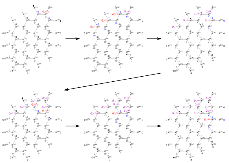
Figure 12. Reconstruction of the potential in the hexagonal lattice

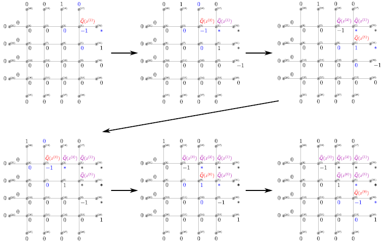
Figure 13. Reconstruction of the potential in the square lattice

(2) Use Lemma 6.3 to construct the data $\widehat{f}$ and the solution $\widehat{u}$ with $\ell=N$. Determine the values of $\widehat{Q}$ on $B_{N}$ by the argument similar to the one in (1).

(3) Assume that all the values of $\widehat{Q}$ on $\{x_{1}+\sqrt{3}x_{2}>a_{k}\}$ are computed. Use Lemma 6.2 to construct the data $\widehat{f}$ and the solution $\widehat{u}$ which takes values $1,-1,1,\cdots$ on $A_{k}$. Use the equation, $\widehat{f}$, the D-N map and the values of $\widehat{Q}$, compute the values $\widehat{u}$ in the region $\{x_{1}+\sqrt{3}x_{2}>a_{k}\}$. Then, calculate $\widehat{Q}$ on $A_{k}$ using the equation.

(4) Assume that all the values of $\widehat{Q}$ on $\{x_{1}+\sqrt{3}x_{2}\geq a_{k}\}\cap\{x_{1}-\sqrt{3}x_{2}<b_{\ell}\}$ are computed. Use Lemma 6.3 to construct the data $\widehat{f}$ and the solution $\widehat{u}$ which takes values $\pm 1$ on $B_{\ell}$. Use the equation to compute the value of $\widehat{Q}$ at $A^{\prime}_{k}\cap B_{\ell}$. This makes it possible to compute $\widehat{Q}$ on $A^{\prime}_{k}$.

(5) Repeat the above procedure until $k=0$.

(6) Rotate the domain, and compute the values of $\widehat{Q}$ at the remaining points by the same procedure as above.

The above reconstruction procedure and that for the case of the square lattice are illustrated in the Figures 12 and 13.

7. Inverse problems for resistor networks

In the previous section, we studied the inversion procedure for the scalar potential from the S-matrix. In this section, we consider the inverse problems for the electric conductivity and graph structure from the S-matrix.This should be compared with the perturbation of Riemannian metric or domain for the case of continuous model.

7.1. Inverse boundary value problem for resistor network

A circular planer graph $G=\{\mathcal{V},\mathcal{E}\}$ is a graph which is imbedded in a disc $D\subset{\bf R}^{2}$ so that its boundary $\partial\mathcal{V}$ lies on the circle $\partial D$ and its interior $\stackrel{{\scriptstyle\circ}}{{\mathcal{V}}}$ is in the topological interior of $D$. A conductivity on $G$ is a positive function $\gamma$ on the edge set $\mathcal{E}$. For $e\in\mathcal{E}$, the value $\gamma(e)$ is called the conductance of $e$, and its inverse $1/\gamma(e)$ the resistance of $e$. Equipped with the conductance, the graph $G$ is called the resistor network. The Laplacian $\widehat{\Delta}_{res}$ is defined by

(7.1) $$\big{(}\widehat{\Delta}_{res}\widehat{u}\big{)}(v)=\sum_{w\in\mathcal{N}_{v}}\gamma(e_{vw})\Big{(}\widehat{u}(w)-\widehat{u}(v)\Big{)},$$

where $e_{vw}$ is an edge with end points $v,w$. Then, for any boundary value $\widehat{f}$, there exists a unique $\widehat{u}$ satisfying

(7.2) $$\left\{\begin{split}&\widehat{\Delta}_{res}\widehat{u}=0\quad{\rm in}\quad\stackrel{{\scriptstyle\circ}}{{\mathcal{V}}},\\ &\widehat{u}=\widehat{f}\quad{\rm on}\quad\partial\mathcal{V}.\end{split}\right.$$

The D-N map $\Lambda_{res}$ is defined by

(7.3) $$\Lambda_{res}\widehat{f}=-\widehat{\Delta}_{res}\widehat{u}\quad{\rm on}\quad\partial{\mathcal{V}},$$

where $\widehat{u}$ is the solution to (7.2). (See [9], [16].)

We compare inverse problems for resistor networks with inverse conductivity problems for continuous models. For a compact manifold $M$ with boundary $\partial M$, the D-N map defined on $\partial M$ is invariant by any diffeomorphism on $M$ leaving $\partial M$ invariant. It is shown that in 2-dimensions the D-N map determines the conductivity up to these diffeomorphisms. For higher dimensions, it is proven under the additional assumption of real-analyticity. Also it is known that the scattering relation (which is defined through the geodesic in $M$ with end points on $\partial M$) determines the simple manifold ([45], [52]). Here, the simple manifold is a compact Riemannian manifold with strictly convex boundary, whose exponential map ${\rm exp}_{x}:{\rm exp}_{x}^{-1}(\overline{M})\to\overline{M}$ is a diffeomorphism.

The above mentioned issues in differential geometry have counter parts in the resistor network. Instead of the diffeomorphism, one uses the notion of criticality and elementary transformation. The geodesics is also extended on the graph. Connection is defined to introduce a mapping between two parts of the boundary. First let us recall these notions.

A path from $v\in\partial{\mathcal{V}}$ to $w\in\partial{\mathcal{V}}$ is a sequence of edges : $e_{i}=e_{i}(v_{i},v_{i+1}),i=0,\cdots,n-1$, such that $v_{0}=v$, $v_{n}=w$, and $v_{i}\ (1\leq i\leq n-1)$ are distinct vertices in $\stackrel{{\scriptstyle\circ}}{{\mathcal{V}}}$. Two sequences of boundary vertices $P=(p_{1},\cdots,p_{k}),Q=(q_{1},\cdots,q_{k})$ are said to be connected through $G$ if there exists a path $c_{i}$ from $p_{i}$ to $q_{i}$, $i=1,\cdots,k$, moreover $c_{i}$ and $c_{j}$ have no vertex in common if $i\neq j$. In this case, the pair $(P,Q)$ is said to be a $k$-connection. The graph $G$ is said to be critical if one removes any edge in $\mathcal{E}$, there exist $k$ and a $k$-connection $(P,Q)$ in $G$ which is no longer connected in the resulting graph $G^{\prime}$ after the removal of the edge. Here, to remove the edge means either to delete the edge leaving end points as two vertices, or to contract the edge letting two end points together into one vertex (see [16], p. 16). An arc $c(t),0\leq t\leq 1$, in $G$ is a union of edges such that $c(t)$ is continuous, and $c(t)\in\partial\mathcal{V}$ if and only if $t=0,1$.

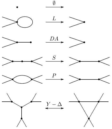
Figure 14. Elementary transformations

The elementary transformations of a planar graph consist of the following 6 operations.

• ($\emptyset$) (Point) means to remove an isolated vertex.

• (L) (Loop) means to remove a loop.

• (DA) (Dead arm) means to remove an edge with end point of degree 1.

• (S) (Series) means to remove a vertex $a$ ($a\not\in\partial{\mathcal{V}}$) of degree 2 and the two adjacent edges and to join the neighboring vertices $b$, $c$ of $a$ by one edge. The conductance of the edge $e_{bc}$ is defined by

  (7.4) $$\gamma(e_{b,c})=\left(\gamma(e_{b,a})^{-1}+\gamma(e_{a,c})^{-1}\right)^{-1}.$$

• (P) (Pararelle) means to replace two edges joining the same vertices $a$ and $b$ by one edge. The conductance is defined by

  (7.5) $$\gamma_{a,b}=\gamma^{\prime}_{a,b}+\gamma^{\prime\prime}_{a,b},$$

  where $\gamma^{\prime}_{a,b}$ and $\gamma^{\prime\prime}_{a,b}$ are the conductances of the double edges.

• ($Y-\Delta$) means to replace a star with 3 branches of center $0$ and edges $(0,1)$, $(0,2)$, $(0,3)$ by one triangle of the vertices 1, 2, 3, and remove the center 0. The conductances are defined by

  (7.6) $$\gamma(e_{i,j})=\frac{\gamma(e_{0,i})\gamma(e_{0,j})}{\gamma(e_{0,1})+\gamma(e_{0,2})+\gamma(e_{0,3})}.$$

The meaning of these graph operations will be clear by Figure 14.

Remark 7.1.

Note that the elementary transformations increase neither the number of vertices nor that of edges. Hence, it does not increase the number of arcs.

Using these notions, it is shown that

Theorem 7.2.

(1) Any circular planar graph is transformed to a critical graph, which is unique within elementary transformations.
(2) Any critical circular planar graph is uniquely determined by its D-N map up to elementary transformations.
(3) Any two circular planar equivalent graphs have the same number of arcs.

For the proof, see Corollary 9.4 and Theorem 9.5 in p. 168 of [16], and Theorem 4 in p. 146 of [12], where the reconstruction procedure of the graph is also explained.

7.2. From the S-matrix to the D-N map for resistor network

7.2.1. Conductivity problem

Let us return to the inverse scattering problem. Assuming that there is no defect, whose meaning will be given in 7.3.2, we can formulate the perturbation of conductivity in the form $\widehat{V}$ in the assumption (B-4). By the arguments in §4, the inverse scattering problem is reduced to the inverse boundary value problem in a bounded domain. Note that from the S-matrix of energy $\lambda$, we obtain the D-N map with energy $\lambda$ associated with the equation (3.29).

7.2.2. Defect problem

We need to pay attention in formulating the inverse boundary value problem in a domain with defect in terms of the resistor network problem. We explain it more precisely. Suppose that we are given a periodic lattice $\Gamma_{0}=\{\mathcal{L}_{0},\mathcal{V}_{0},\mathcal{E}_{0}\}$ as in §2 satisfying the assumptions (A-1) $\sim$ (A-4). We perturb $\Gamma_{0}$ locally, and let the resulting graph $\Gamma=\{\mathcal{V},\mathcal{E}\}$ satisfy the assumptions (B-1) $\sim$ (B-4). Let $\mathcal{V}_{int}$ be the associated interior domain. Assume that $\mathcal{V}_{int}$ is a planar graph in the sense of Subsection 7.1, and denote it by $\mathcal{V}_{def}$. To make this perturbation consistent with the previous arguments, we assume that

$$\sharp\{w\in\,\stackrel{{\scriptstyle\circ}}{{\mathcal{V}_{def}}}\ ;\ w\sim v\},\quad v\in\partial\mathcal{V}_{def},$$

is a constant on $\partial\mathcal{V}_{def}$ which is denoted by $\mu_{0}$. In order to apply Theorem 7.2 to our problem, we take

$$\gamma(e_{vw})=1.$$

Then we have

$$-\widehat{\Delta}_{res}=\mathrm{deg}_{\mathcal{V}_{def}}(\cdot)(\widehat{\Delta}_{\Gamma}-1)\quad\text{in}\quad\stackrel{{\scriptstyle\circ}}{{\mathcal{V}_{def}}}.$$

Hence the equation (7.2) is rewritten as

(7.7) $$\left\{\begin{split}&(-\widehat{\Delta}_{\Gamma}+1)\widehat{u}=0\quad\text{in}\quad\stackrel{{\scriptstyle\circ}}{{\mathcal{V}_{def}}},\\ &\widehat{u}=\widehat{f}\quad{\rm on}\quad\partial\mathcal{V}_{def},\end{split}\right.$$

Note that $-\widehat{\Delta}_{\Gamma}$ is self-adjoint on $\ell^{2}(\stackrel{{\scriptstyle\circ}}{{\mathcal{V}_{def}}})$ equipped with the inner product

$$(\widehat{f},\widehat{g})_{\ell^{2}(\stackrel{{\scriptstyle\circ}}{{\mathcal{V}_{def}}})}=\sum_{v\in\stackrel{{\scriptstyle\circ}}{{\mathcal{V}_{def}}}}\widehat{f}(v)\overline{\widehat{g}(v)}\mathrm{deg}_{\mathcal{V}_{def}}(v),$$

where $\widehat{f}(v)=\widehat{g}(v)=0$ for any $v\in\partial\mathcal{V}_{def}$. This operator is denoted by $-\widehat{\Delta}_{\Gamma,\mathcal{V}_{def}}$.

Lemma 7.3.

We have $\ -1\not\in\sigma(-\widehat{\Delta}_{\Gamma,\mathcal{V}_{def}})$.

Proof. Suppose $-1\in\sigma(-\widehat{\Delta}_{\Gamma,\mathcal{V}_{def}})$. Then there exists a function $\widehat{u}$ satisfying the equation

$$\left\{\begin{split}&\widehat{\Delta}_{res}\widehat{u}=0\quad\text{in}\quad\stackrel{{\scriptstyle\circ}}{{\mathcal{V}_{def}}},\\ &\widehat{u}=0\quad{\rm on}\quad\partial\mathcal{V}_{def},\end{split}\right.$$

However, the maximum principle for harmonic functions associated with $\widehat{\Delta}_{res}$ implies that $\widehat{u}$ must vanish in $\stackrel{{\scriptstyle\circ}}{{\mathcal{V}_{def}}}$ (see Theorem 3.2 and Corollary 3.3 in [16]). This is a contradiction. ∎

The results in §2 $\sim$ §5 also hold for this perturbed system. To study $\mathcal{V}_{def}$, in view of (7.7), we have to consider the operator $-\widehat{\Delta}_{\Gamma,\mathcal{V}_{def}}$ and its D-N map with $\lambda=-1$. However, we have $-1\in\sigma_{e}(\widehat{H})\cap\mathcal{T}$ in some examples of lattices satisfying the above assumptions. For these reasons, we pick up some cases in which we can compute the D-N map $\Lambda_{int}(\lambda)$ from the S-matrix of $\widehat{H}=-\widehat{\Delta}_{\Gamma}$.

Case 1. If $\lambda\in\sigma_{e}(\widehat{H})\setminus\mathcal{T}$, there is no problem, and we can apply our previous arguments.

Case 2. Let $\lambda\not\in\sigma(-\widehat{\Delta}_{\Gamma,\mathcal{V}_{def}})$. Take any open set $\mathcal{O}\subset\sigma_{e}(\widehat{H})\setminus\mathcal{T}$. If we are given the S-matrix for all energy $\mu\in\mathcal{O}$, we can compute the D-N map for $-\widehat{\Delta}_{\Gamma,\mathcal{V}_{def}}-\mu$ with $\mu\in\mathcal{O}\setminus\sigma(-\widehat{\Delta}_{\Gamma,\mathcal{V}_{def}})$. Since the D-N map $\Lambda_{int}(\mu)$ is meromorphic with respect to the energy $\mu$, using the analytic continuation and taking $\mu=\lambda$, we can compute the D-N map $\Lambda_{int}(\lambda)$ for $\widehat{\Delta}_{res}$.

Case 3. In practical applications, it often happens that $\lambda$ is an end point of $\sigma_{e}(\widehat{H})$ as above. For example, this is the case for the perturbation of the hexagonal lattice. In view of Lemma 7.3, the D-N map for $-\widehat{\Delta}_{\Gamma,\mathcal{V}_{def}}-\mu$ is continuous with respect to $\mu$ when $\mu$ is close to $\lambda$. Therefore, choosing a sequence $\mu_{j}$ convergent to $\lambda$, one can compute the D-N map $\Lambda_{int}(\lambda)$ from the S-matrices $S(\mu_{j})$ for $j\geq 1$.

The above arguments have a general character and work for many lattices satisfying our assumptions (A-1) $\sim$ (A-4) and (B-1) $\sim$ (B-4). Thus, when we perturb a bounded part of these lattices by a planer network,

we can determine the perturbation as a planer network

by using Theorem 7.2.

Main barriers for this fact are the Rellich type theorem and the unique continuation property for the associated spectral problems. In Theorem 5.10 of [4], we summarized examples of the lattices having this property. Therefore, when we perturb a bounded part of square, triangular, and hexagonal lattices by removing a finite number of edges in such a way that the unique continuation property holds in the remaining part (see [34] and the Figures 11 and 12 in [4]), we can determine the network.

As is seen from the definition, the elementary transformations are of topological nature, and its physical realization is not an obvious problem. Therefore we must be careful in the application of above results, which we shall discuss in the next subsection.

7.3. Inverse resistor network problem in the hexagonal lattice

7.3.1. Conductivity

To study the conductivity problem, in the assumptions (B-1) $\sim$ (B-4), we take $\mathcal{V}_{int}$ to be a sufficiently large planar graph so that the conductivity is constant on $\mathcal{V}_{ext}$. Then by Theorem 7.2, the D-N map (7.3) determines the Laplacian on $\mathcal{V}_{int}$ as a planar network. Since the S-matrix with energy $\lambda$ determines the associated D-N map, taking note that the S-matrix and the D-N map are analytic with respect to the energy $\lambda$, we can compute the D-N map (7.3) from the S-matrix for all energies. We have thus proven the following theorem.

Theorem 7.4.

The conductivity of the periodic hexagonal lattice is determined by the S-matrix of all energies.

7.3.2. Defects

By defects we mean to delete some edges and to remove isolated vertices. Consider, for example, the simplest case in which only one edge, say the edge with end points $a$ and $d$ in Figure 24, is removed. Our main idea of detecting defects consists in using the solution $\widehat{u}$ given in Lemmas 6.2 and 6.3 with $\widehat{Q}=-\lambda$. As will be discussed in the proof of Lemma 7.9, one can detect the defect by observing the D-N map, or equivalently the S-matrix. Before going to the general case, we prepare a little more notion.

7.3.3. Convex polygon

There are 3 kinds of straight lines in the hexagonal lattice (Figure 16, 16, 18).

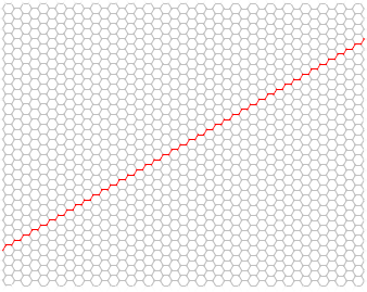
Figure 15. Straight line 1 in the hexagonal lattice

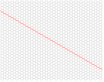
Figure 16. Straight line 2 in the hexagonal lattice

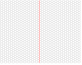
Figure 17. Straight line 3 in the hexagonal lattice

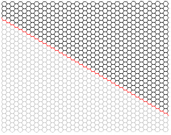
Figure 18. Half space in the hexagonal lattice

Then a half-space is defined as in Figure 18.

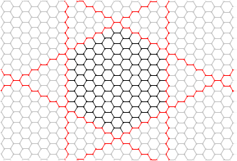
Figure 19. Hexagonal honeycomb in the hexagonal lattice

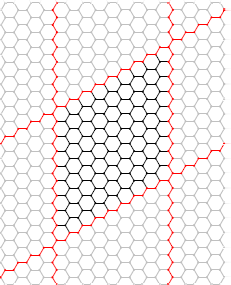
Figure 20. Hexagonal parallelogram in the hexagonal lattice

Let

(7.8) $$\omega=e^{\pi i/3},$$

and put

(7.9) $$\left\{\begin{split}&v_{1}=1+\omega=(3+\sqrt{3}i)/2,\\ &v_{2}=\omega(1+\omega)=\sqrt{3}i,\\ &v_{3}=\omega^{2}(1+\omega)=(-3+\sqrt{3}i)/2.\end{split}\right.$$

Let $U_{h}$ be the unit hexagon, which is defined to be a hexagon with vertices $\omega^{j},j=0,1,\cdots,5$. For $i,j=1,2,3$, $i\neq j$, and $k\in{\bf Z}$, define the half-space $H_{i,j,k}^{(\pm)}$ by

(7.10) $$H^{(+)}_{i,j,k}={\mathop{\cup}_{l=-\infty}^{\infty}}\,{\mathop{\cup}_{m\geq k}}\left\{mv_{i}+lv_{j}+U_{h}\right\},$$

(7.11) $$H^{(-)}_{i,j,k}={\mathop{\cup}_{l=-\infty}^{\infty}}\,{\mathop{\cup}_{m\leq k}}\left\{mv_{i}+lv_{j}+U_{h}\right\}.$$

By a convex polygon, we mean an intersection of finite number of half-spaces. In the following, we consider only finite convex polygons. See e.g. Figures 20 and 20. As typical examples of convex polygon, we consider the following two types of domain : hexagonal honeycomb and hexagonal parallelogram. Figure 20 suggests the former, and Figure 20 the latter.

Taking $n$ large enough, we construct the 0th vertical block

$$B_{0}={\mathop{\cup}_{k=-n}^{n}}\left(U_{h}+k\sqrt{3}i\right).$$

We next put $U_{h}^{\prime}=U_{h}+\frac{\sqrt{3}}{2}i$, and make the 1st block

$$B_{\pm 1}={\mathop{\cup}_{k=-n}^{n-1}}\left(U_{h}^{\prime}+k\sqrt{3}i\pm\frac{3}{2}\right).$$

The 2nd block $B_{\pm 2}$ consists of the $2n-1$ number of translated $U_{h}$’s. Repeating this procedure $n$ times, we obtain the hexagonal honeycomb. Look at Figure 21 and imagine the case without hole inside. It is the hexagonal honeycomb. We attach edges to the vertices with degree 2 on it and also the new vertices on the end points of these edges (white dots in Figure 21), we define the hexagonal honeycomb with boundary.

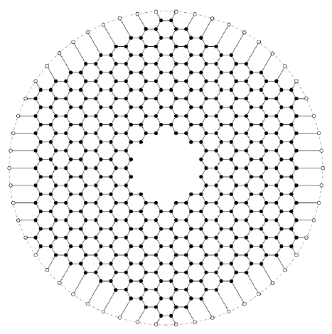
Figure 21. Hexagonal honeycomb

We next define another block

$$B^{\prime}_{0}={\mathop{\cup}_{k=0}^{m}}\left(U_{h}+k\sqrt{3}i\right),$$

and translate $B^{\prime}_{0}$ by $\ell(1+\omega)$ :

$$B^{\prime}_{\ell}=B^{\prime}_{0}+\ell(1+\omega).$$

We define

$$P_{N}={\mathop{\cup}_{\ell=-N}^{N}}B^{\prime}_{\ell},$$

and call it a hexagonal parallelogram (cf. Figure 8). When $N=\infty$, it is called graphene nanoribbon (see [40]).

Letting $e_{1},e_{2}$ be the edges such that $o(e_{1})=\omega^{2},t(e_{1})=\omega$, $o(e_{2})=\omega,t(e_{2})=2\omega$, we put

$$L_{12,k}=e_{1}\cup e_{2}+k\sqrt{3}i,\quad-1\leq k\leq m,$$

which are the horizontal edges of $B^{\prime}_{k}$. We put

$$Z_{k}={\mathop{\sum}_{\ell=-\infty}^{\infty}}\left(L_{12,k}+\ell(1+\omega)\right),\quad-1\leq k\leq m,$$

and call it a parallel line in $P_{\infty}$.

Lemma 7.5.

A convex polygon with boundary is a critical graph.

Proof. Since the proof is similar in all cases, we give the proof for the hexagonal honeycomb. Letting $\mathcal{H}$ be a hexagonal honeycomb with boundary, we remove an edge from $\mathcal{H}$. By rotating $\mathcal{H}$, we can assume that the removed edge $e_{r}$ is horizontal. Let $B$ be the block of $\mathcal{H}$ containing $e_{r}$. By translation, we can assume that the bottom of the block $B$ is the edge with vertices $\omega^{4}$ and $\omega^{5}$. By translating $B$ to the directions $\pm(1+\omega)$, we obtain an infinite hexagonal parallelogram $P_{\infty}$, and the associated parallel lines $Z_{k}$, $-1\leq k\leq m$. Let $p_{k},q_{k}$ be the intersection of $Z_{k}$ with $\partial\mathcal{H}$, where $p_{k}$ is the left point of intersection, and $q_{k}$ the right point of intersection. Then $(P,Q)$, where $P=(p_{-1},\cdots,p_{m})$ and $Q=(q_{-1},\cdots,q_{m})$, is an $(m+2)$-connection of the graph $\mathcal{H}$. Then, if we remove one horizontal edge from $B$, it is no longer a connection, since $B$ has only $m+1$ horizontal edges. ∎

We define the outer wall of a convex polygon taking the hexagonal honeycomb as an example. From the hexagonal honeycomb, we remove all the edges inside and leave only the edges on the periphery. We attach the edge to the vertices with inner angle $2\pi/3$ and a vertex at its end point. Let us call the resulting graph outer wall of the hexagonal honeycomb with boundary (Figure 23). We can also define, for example, outer wall of the hexagonal parallelogram with boundary (Figure 23). It is another critical case.

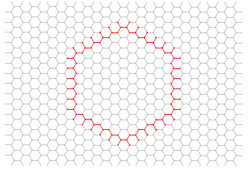
Figure 22. Outer wall of the hexagonal honeycomb with boundary

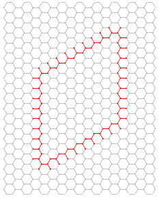
Figure 23. Outer wall of the hexagonal parallelogram with boundary

Lemma 7.6.

The outer wall of convex polygon with boundary is a critical graph.

Proof. As above, we give the proof for the hexagonal honeycomb. Take two vertices $p_{1},q_{1}$ on the boundary top of the hexagonal honeycomb, $p_{1}$ being the right to $q_{1}$. Take $p_{2},q_{2}$ on the bottom, $p_{2}$ being left to $q_{2}$. Then, $P=\{p_{1},p_{2}\}$, $Q=\{q_{1},q_{2}\}$ are 2-connections. Let $a,b$ be the end points of the edges emanating from $p_{1},q_{1}$, respectively. Then, if we delete the edge $e_{ab}$, $P$ and $Q$ are no longer 2-connected. ∎

In order to detect several defects, we restrict ourselves to the case in which the defects are of the shape of hexagonal honeycomb of one connected component and every component is separated from each other.

Theorem 7.7.

Let the defect $\mathcal{D}$ be of the form $\mathcal{D}=\cup_{i=1}^{N}\mathcal{D}_{i}$, where $\mathcal{D}_{i}\cap\mathcal{D}_{j}=\emptyset$ if $i\neq j$ and one of $\mathcal{D}_{i}$’s is a convex polygon. Assume that the unique continuation property holds on the exterior domain of $\stackrel{{\scriptstyle\circ}}{{\mathcal{D}}}$. Then the set $\{\lambda\in\sigma_{e}(\widehat{H})\,;\,S(\lambda)=I\}$ is of measure $0$.

Proof. Let $\mathcal{D}_{ow}=\cup_{i=1}^{N}\mathcal{D}_{i,ow}$, where $\mathcal{D}_{i,ow}$ is the outer wall of $\mathcal{D}_{i}$. In the assumptions (B-1) $\sim$ (B-4), we take $\mathcal{V}_{int}=\mathcal{D}_{ow}$, and $\mathcal{V}_{ext}$ to be the domain exterior to $\stackrel{{\scriptstyle\circ}}{{\mathcal{D}}}$. Then, $\mathcal{V}=\mathcal{V}_{ext}\cup\mathcal{V}_{int}$. Note that if $\mathcal{D}_{ow}$ is replaced by $\mathcal{D}$, the associated S-matrix is the identity. Note that we can apply results in §4 to the D-N maps for $\mathcal{D}_{ow}$ and $\mathcal{D}$.

Suppose there exists a set of positive measure $E\subset\sigma_{e}(\widehat{H})$ such that $S(\lambda)=I$ for $\lambda\in E$. By taking $\mathcal{V}_{int}$ to be $\mathcal{D}_{ow}$ and $\mathcal{D}$, we see that the D-N map for $\mathcal{D}_{ow}$, which is the product of each D-N map for $\mathcal{D}_{i,ow}$, coincides with that for $\mathcal{D}$. Suppose $\mathcal{D}_{1}$ is a convex polygon. Since $\mathcal{D}_{1,ow}$ and $\mathcal{D}_{1}$ are critical, Theorem 7.2 and Lemmas 7.5 and 7.6 imply that they coincide as a planar graph. In particular, they must have the same number of arcs, which is not true. This proves the theorem. ∎

This theorem asserts that one can detect the existence of defects from the knowledge of the S-matrix for all energies, however it does not tell us its location. In the next subsection, we find it by employing a different idea.

7.4. Probing waves

Let $\stackrel{{\scriptstyle\circ}}{{\mathcal{D}}}$ be a convex polygon. Take a sufficiently large hexagonal parallelogram $\mathcal{V}_{0,int}$ which contains $D$, and put

(7.12) $$\mathcal{V}_{def}=\mathcal{V}_{0,int}\setminus\stackrel{{\scriptstyle\circ}}{{\mathcal{D}}}.$$

In the following, $\Sigma$ denotes $\partial\mathcal{V}_{0,int}=\partial\mathcal{V}_{def}$ and $(\Sigma)_{T}$, $(\Sigma)_{B}$, $(\Sigma)_{R}$ and $(\Sigma)_{L}$ denote the top, bottom, right and left side of $\Sigma$, respectively. We consider the following problem ${\mathcal{H}}_{def}$ on the region with defects

(7.13) $$\left\{\begin{split}&(-\widehat{\Delta}_{\Gamma}-\lambda)\widehat{u}=0\quad\text{in}\quad\stackrel{{\scriptstyle\circ}}{{\mathcal{V}_{def}}},\\ &\widehat{u}=\widehat{f}\quad\text{on}\quad\Sigma,\end{split}\right.$$

and the problem $\mathcal{H}_{0}$ on the region without defects

(7.14) $$\left\{\begin{split}&(-\widehat{\Delta}_{\Gamma_{0}}-\lambda)\widehat{u}_{0}=0\quad\text{in}\quad\stackrel{{\scriptstyle\circ}}{{\mathcal{V}_{0,int}}},\\ &\widehat{u}_{0}=\widehat{f}\quad\text{on}\quad\Sigma.\end{split}\right.$$

We assume :

(E)  The number $\lambda$ is not equal to 0, and also neither an eigenvalue of the Dirichlet problem (7.13) nor that of (7.14).

Then, the boundary value problems (7.13) and (7.14) can be solved uniquely for any data $\widehat{f}$. Let $\Lambda(\mathcal{H}_{0})$ and $\Lambda({\mathcal{H}}_{def})$ be the D-N maps for $\mathcal{H}_{0}$ and $\mathcal{H}_{def}$, respectively. As is seen in Figure 8, there are two types of vertices on $\partial\mathcal{D}$. One is the vertex $v\in\partial\mathcal{D}$ with $\mathrm{deg}_{\mathcal{V}_{def}}(v)=3$ and inner angle $2\pi/3$, and the other is the vertex $v^{\prime}\in\partial\mathcal{D}$ with $\mathrm{deg}_{\mathcal{V}_{def}}(v^{\prime})=2$ and inner angle $4\pi/3$.

Let $A_{k}$, $A^{\prime}_{k}$ be the lines in Figure 10 in §6.2, and take $\alpha_{k,0}\in A_{k}\cap(\Sigma)_{T}$, $\alpha_{k,\ell^{\prime}}\in A_{k}\cap(\Sigma)_{R}$. Let $\widehat{u}_{0,k}$ be the solution of (7.14) with partial Dirichlet data $\widehat{f}$ such that

(7.15) $$\left\{\begin{split}&\widehat{f}(\alpha_{k,0})=1,\\ &\widehat{f}(\alpha_{k,\ell^{\prime}})=(-1)^{\ell^{\prime}},\\ &\widehat{f}(v)=0\quad\text{for}\quad v\in\Sigma\setminus((\Sigma)_{R}\cup\{\alpha_{k,0}\}),\end{split}\right.$$

and partial Neumann data vanishing on $(\Sigma)_{L}$. Lemma 6.2 implies that $\widehat{u}_{k,0}$ exists uniquely on $\mathcal{V}_{0,int}$ and satisfies

(7.16) $$\widehat{u}_{0,k}(\alpha_{k,\ell})=\left\{\begin{split}&(-1)^{\ell}\quad{\rm for}\quad\ell=0,1,\cdots,\ell^{\prime},\\ &\widehat{u}_{0,k}(x_{1}+ix_{2})=0\quad{\rm for}\quad x_{1}+\sqrt{3}x_{2}<a_{k}.\end{split}\right.$$

This solution $\widehat{u}_{0,k}$ is an analogue of the exponentially growing solution introduced in [22], [59]. We put

(7.17) $$\widehat{f}_{k}=\widehat{u}_{0,k}\big{|}_{\Sigma},$$

and let $\widehat{u}_{k}$ be the solution of (7.13) with $\widehat{f}=\widehat{f}_{k}$.

Lemma 7.8.

We take $N$ large enough, and starting from $k=N$, let $k$ vary downwards. Let $m$ be the largest $k$ such that $A_{k}$ meets $\mathcal{D}$. Then, $\widehat{u}_{0,k}=\widehat{u}_{k}$ on $\mathcal{V}_{def}$ for $k\geq m$.

Proof. Note that $A_{m}$ passes through only vertices $v\in\partial\mathcal{D}$ with $\mathrm{deg}_{\mathcal{V}_{def}}(v)=3$ and inner angle $2\pi/3$. Then, for any function $\widehat{u}$ on $\mathcal{V}_{0,int}$, we have $((-\widehat{\Delta}_{\Gamma}+1)\widehat{u})(x_{1}+ix_{2})=((-\widehat{\Delta}_{\Gamma_{0}}+1)\widehat{u})(x_{1}+ix_{2})$ for any $x_{1}+ix_{2}\in\stackrel{{\scriptstyle\circ}}{{\mathcal{V}_{def}}}$ with $x_{1}+\sqrt{3}x_{2}\geq a_{m}$. By virtue of this equality and $\widehat{u}_{0,k}(x_{1}+ix_{2})=0$ for $x_{1}+\sqrt{3}x_{2}<a_{k}$, $\widehat{u}_{0,k}$ is a solution of (7.13) with $\widehat{f}=\widehat{f}_{k}$ if $k\geq m$. Since (7.13) is uniquely solvable, we have $\widehat{u}_{k}=\widehat{u}_{0,k}$. ∎

We have now arrived at the following probing algorithm for the defects $\mathcal{D}$ of convex polygon in the hexagonal lattice.

Lemma 7.9.

Let $f_{k}$ be defined by (7.17), and $m$ the number defined in Lemma 7.8. Then, we have

(7.18) $$\Lambda(\mathcal{H}_{def})\widehat{f}_{k}=\Lambda(\mathcal{H}_{0})\widehat{f}_{k},\quad k\geq m,$$

and

(7.19) $$\Lambda(\mathcal{H}_{def})\widehat{f}_{k}\not=\Lambda(\mathcal{H}_{0})\widehat{f}_{k},\quad k=m-1.$$

Proof. For $k\geq m$, (7.18) is a direct consequence of Lemma 7.8. Let us show (7.19). As is illustrated in Figure 24, $A_{m-1}$ passes through a vertex $a\in\partial\mathcal{D}$ with $\mathrm{deg}_{\mathcal{V}_{def}}(a)=2$ and inner angle $4\pi/3$. Let $b,e\in\stackrel{{\scriptstyle\circ}}{{\mathcal{V}_{def}}}$ be the adjacent vertices of $a$.

Figure 24. Probing for defects

Assume that $\Lambda(\mathcal{H}_{def})\widehat{f}_{m-1}=\Lambda(\mathcal{H}_{0})\widehat{f}_{m-1}$. Then, by the same reasoning as in the proof of Lemma 7.8, we have $\widehat{u}_{m-1}=\widehat{u}_{0,m-1}$ on $\mathcal{V}_{def}$.

Computing the equation $(-\widehat{\Delta}_{\Gamma}-\lambda)\widehat{u}_{m-1}=0$ at the above vertex $a\in A_{m-1}\cap\partial\mathcal{D}$, we have

(7.20) $$-\frac{1}{2}\left(\widehat{u}_{m-1}(b)+\widehat{u}_{m-1}(c)\right)-\lambda\widehat{u}_{m-1}(a)=0.$$

Similarly, the equation $(-\widehat{\Delta}_{\Gamma_{0}}+1)\widehat{u}_{0,m-1}=0$ at $a\in A_{m-1}\cap\partial\mathcal{D}$ is

(7.21) $$-\frac{1}{3}\left(\widehat{u}_{0,m-1}(b)+\widehat{u}_{0,m-1}(c)+\widehat{u}_{0,m-1}(d)\right)-\lambda\widehat{u}_{0,m-1}(a)=0,$$

where $d=a+\omega^{5}$. Putting $\alpha_{m-1,\ell}=a$ in Figure 10, we have $\widehat{u}_{0,m-1}(a)=(-1)^{\ell}$ and $\widehat{u}_{0,m-1}(d)=0$. However, (7.20) and (7.21) imply $\widehat{u}_{m-1}(a)=\widehat{u}_{0,m-1}(a)=0$, since $\widehat{u}_{m-1}=\widehat{u}_{0,m-1}$ on $\mathcal{V}_{def}$. This is a contradiction. ∎

Let us pay attention to a relation between Lemma 7.9 and the partial data problem for the Laplacian on $\mathcal{V}_{def}$. In fact, the pair $((\Sigma)_{L},(\Sigma)_{R})$ is an $(N+1)$-connection for $\mathcal{H}_{0}$ and is broken for $\mathcal{H}_{def}$. Then $\mathcal{H}_{0}$ is critical. It follows that the submatrix of $\Lambda(\mathcal{H}_{def})$ mapping from $(\Sigma)_{R}$ to $(\Sigma)_{L}$ (in the sense of Lemma 6.1) is singular. Therefore, the partial data problem on $\mathcal{V}_{def}$ in the sense of Lemma 6.1 is overdetermined, hence is ill-posed.

We consider the probing for the defects $\mathcal{D}=\bigcup_{j=1}^{s}\mathcal{D}_{j}$ where each $\mathcal{D}_{j}$ is a convex polygon such that $\mathcal{D}_{j}\cap\mathcal{D}_{k}=\emptyset$ if $j\not=k$. Our method can be applied also to this case.

Lemma 7.10.

For $\mathcal{D}=\bigcup_{j=1}^{s}\mathcal{D}_{j}$, the assertion of Lemma 7.9 holds.

Proof. For $k\geq m$, the proof is completely the same. For $k=m-1$, we have $\widehat{u}_{0,k}=\widehat{u}_{k}$ in $\mathcal{V}_{def}\setminus\,\stackrel{{\scriptstyle\circ}}{{C(\mathcal{D})}}$ where $C(\mathcal{D})$ is the hexagonal convex hull of $\mathcal{D}$. It then leads to a contradiction at a vertex $v\in\partial C(\mathcal{D})\cap\partial\mathcal{D}$ with degree $2$ as in the proof of Lemma 7.9. ∎

A similar probing procedure is possible by using $B_{\ell}$ in Figure 11. We have only to rotate the domains $\mathcal{H}_{0}$ and $\mathcal{H}_{def}$ in the above arguments. Then, one can enclose the region with defects by the convex hull $C(\mathcal{D})$.

In Lemma 4.7, we take $\mathcal{V}_{int,1}$ to be the interior domain without defects, and $\mathcal{V}_{int,2}$ with defects. Using (4.6), we define $\phi_{k}\in M_{\lambda}$ by

(7.22) $$\phi_{k}=\big{(}\widehat{J}^{(-)}(\lambda)^{\ast}\big{)}^{-1}B^{(+)}_{\Sigma,0}(\lambda)\widehat{f}_{k}.$$

Then we have

(7.23) $$\widehat{f}_{k}=\big{(}B^{(+)}_{\Sigma,0}(\lambda)\big{)}^{-1}\widehat{I}^{(-)}(\lambda)^{\ast}\phi_{k},$$

where $B^{(+)}_{\Sigma,0}$ is defined by (3.36) for $\mathcal{V}_{int,1}$. Letting $A(\lambda)$ be the scattering amplitude for the lattice with defects, and recalling that the scattering amplitude vanishes for the case without defects, we have, in view of Lemmas 4.7 and 7.10,

(7.24) $$\left\{\begin{split}&A(\lambda)\phi_{k}=0,\quad{\rm if}\quad k\geq m,\\ &A(\lambda)\phi_{k}\neq 0,\quad{\rm if}\quad k=m-1.\end{split}\right.$$

We have thus obtained the following theorem.

Theorem 7.11.

If the set $\mathcal{D}$ of defects consists of a finite number of convex polygons, its convex hull $C(\mathcal{D})$ can be computed from the S-matrix $S(\lambda)$ for an arbitrarily fixed energy $\lambda\in\sigma_{e}(\widehat{H})\setminus{\mathcal{T}}$ satisfying the assumption (E).

References

- [1] S. Agmon, Spectral properties of Schrödinger operators and scattering theory, Ann. Scuola Norm. Sup. Pisa 2 (1975), 151-218.
- [2] S. Agmon and L. Hörmander, Asymptotic properties of solutions of differential equations with simple characteristics, J. d’Anal. Math. 30 (1976), 1-38.
- [3] K. Ando, Inverse scattering theory for discrete Schrödinger operators on the hexagonal lattice, Ann. Henri Poincaré, 14 (2013), 347-383.
- [4] K. Ando, H. Isozaki and H. Morioka, Spectral properties of Schrödinger operators on perturbed lattices, Ann. Henri Poincaré 17 (2016), 2103-2171.
- [5] D. Burago, S. Ivanov and Y. Kurylev, A graph discretization of the Laplace-Beltrami operator, J. Spectr. Theory 4 (2014), 675-714.
- [6] A. P. Calderón, On an inverse boundary value problem, Seminar on Numerical Analysis and its Applications to Continuum Physics, Soc. Brazileira deMathematica, Rio de Janeiro (1980), 65-73.
- [7] K. Chadan, D. Colton, L. Päivärinta and W. Rundell, An Introduction to Inverse Scattering and Inverse Boundary Value Porblems, SIAM, Philadelphia, (1997).
- [8] R. K. Chung, Spectral Graph Theory, Amer. Math. Soc., Providence, Rhode-Island (1997).
- [9] Y. Colin de Verdière, Réseaux électriques planaires I, Commentarii Math. Helv., 69 (1994), 351-374.
- [10] Y. Colin de Verdière, Cours Spécialisés 4, Spectre de Graphes, Soc. Math. de France (1998).
- [11] Y. Colin de Verdière and T. Françoise, Scattering theory for graphs isomorphic to a regular tree at infinity, J. Math. Phys. 54 (2013), 063502.
- [12] Y. Colin de Verdière, I. de Gitler and D. Vertigan, Réseaux électriques planaires II, Commentarii Math. Helv., 71 (1996), 144-167.
- [13] J. C. Cuenin and H. Siedentop, Dipoles in graphene have infinitely many bound states, J. Math. Phys. 55 (1204), 122304.
- [14] E. B. Curtis and J. A. Morrow, Determining the resistors in a network, SIAM J. Appl. Math. 50 (1990), 918-930.
- [15] E. B. Curtis and J. A. Morrow, The Dirichlet to Neumann map for a resistor network, SIAM J. Appl. Math. 51 (1991), 1011-1029.
- [16] E. B. Curtis and J. A. Morrow, Inverse Problems for Electrical Networks, World Scientific, Singapore-New Jersey-London-Hong Kong (2000).
- [17] E. B. Curtis, E. Mooers and J. A. Morrow, Finding the conductors in circular networks, Math. Modeling Numer. Anal. 28 (1994), 781-813.
- [18] E. B. Curtis, D. Ingerman and J. A. Morrow, Circular planar graphs and resisitor networks, Lin. Alg. and its Appl. 283 (1998), 115-150.
- [19] J. Dodziuk, Difference equations, isoperimetric inequality and transience of certain random walks, Trans. Amer. Math. Soc., 284 (1984), 787-794.
- [20] M. S. Eskina, The direct and the inverse scattering problem for a partial difference equation, Soviet Math. Doklady, 7 (1966), 193-197.
- [21] L. D. Faddeev, Uniqueness of the inverse scattering problem, Vestnik Leningrad Univ. 11 (1956), 126-130.
- [22] L. D. Faddeev, Increasing solutions of the Schrödinger eqations, Sov. Phys. Dokl. 10 (1966), 1033-1035.
- [23] L. D. Faddeev, Inverse problem of quantum scattering theory, J. Sov. Math. 5 (1976), 334-396.
- [24] C. Gérard and F. Nier, The Mourre theory for analytically fibred operators, J. Funct. Anal. 152 (1989), 202-219.
- [25] J. González, F. Guiner and M. A. H. Vozmediano, The electronic spectrum of fullerens from the Dirac equation, Nuclear Phys. B 406 (1993), 771-794.
- [26] Y. Higuchi and T. Shirai, Some spectral and geometric properties for infinite graphs, Contemp. Math. 347 (2004), 29-56.
- [27] Y. Higuchi and Y. Nomura, Spectral structure of the Laplacian on a covering graph, Euro. J. of Combinatrics, 30 (2009), 570-585.
- [28] F. Hiroshima, I. Sakai, T. Shirai and A. Suzuki, Note on the spectrum of discrete Schrödinger operators, J. Math-for-Industry 4 (2012), 105-108.
- [29] L. Hörmander, The Analysis of Linear Partial Differential Operators III, Pseudodifferential operators, Springer Verlag, Berlin-Heidelberg-New York-Tokyo (1985).
- [30] M. Ikehata, Reconstruction of obstacles from boundary measurements, Wave Motion 30 (1999), 205-223.
- [31] M. Ikehata, Inverse scattering problems and the enclosure method, Inverse Problems 20 (2004), 533-551.
- [32] H. Isozaki, Inverse spectral theory, in Topics In The Theory of Schrödinger Operators, eds. H. Araki, H. Ezawa, World Scientific (2003), pp. 93-143.
- [33] H. Isozaki and E. Korotyaev, Inverse problems, trace formulae for discrete Schrödinger operators, Ann. Henri Poincaré, 13 (2012), 751-788.
- [34] H. Isozaki and H. Morioka, A Rellich type theorem for discrete Schrödinger operators, Inverse Problems and Imaging, 8 (2014), 475-489.
- [35] H. Isozaki and H. Morioka, Inverse scattering at a fixed energy for discrete Schrödinger operators on the square lattice, Ann. Inst. Fourier 65 (2015), 1153-1200.
- [36] S. T. Kuroda, Scattering theory for differential operators, I, II, J. Math. Soc. Japan 25 (1973), 75-104, 222-234.
- [37] G. M. Khenkin and R. G. Novikov, The -equation in the multi-dimensional inverse scattering problem, Russian Math. Surveys 42 (1087), 109-180.
- [38] T. Kobayashi, K. Ono and T. Sunada, Periodic Schrödinger operators on a manifold, Forum Math. 1 (1989), 69-79.
- [39] T. Kondo, S. Casolo, T. Suzuki, T. Shikano, M. Sakurai, Y. Harada, M. Saito, M. Oshima, M. Trioni, G. Tantardini and J. Nakamura, Atomic-scale characterization of nitrogen-dopted graphite : Effects of dopant nitrogen on the local electronic structure of the surrounding carbon stoms, Phyisical Review B 86, 035436 (2012).
- [40] E. Korotyaev and A. Kutsenko, Zigzag nanoribbons in external electric fields, Asymptotic Anal. 66 (2010), 187-206.
- [41] E. Korotyaev and N. Saburova, Schrödinger operators on periodic graphs, J. Math. Anal. Appl. 420 (2014), 576-611.
- [42] M. Kotani, T. Shirai, and T. Sunada, Asymptotic behavior of the transition probability of a random walk on an infinite graph, J. Funct. Anal. 159 (1998), 664-689.
- [43] P. Kuchment and O. Post, On the spectra of carbon nano-structures, Commun. Math. Phys. 275 (2007), 805-826.
- [44] B. Mohar and W. Woess, A survey on spactra of infinite graphs, Bull. London Math. Soc. 21 (1989), 209-234.
- [45] R. G. Muhometov, The problem of recovery of a two-dimensional Riemannian metric and integral geometry, Soviet Math. Dokl. 18 (1977), 27-31.
- [46] A. Nachman, Reconstruction from boundary measurements, Ann. of Math. 128 (1988), 531-576.
- [47] A. Nachman, Global uniqueness for a two-dimensional inverse boundary value problem, Ann. of Math. 143 (1996), 71-96.
- [48] S. Nakamura, Modified wave operators for discrete Schrödinger operators with long-range perturbations, J. Math. Phys. 55 (2014), 112101.
- [49] A. H. C. Neto, F. Guiner, N. M. R. Peres, K. S. Novoselov and A. K. Geim, The electronic properties of graphene, Rev. Mod. Phys. 81 (2009), 109-162.
- [50] R. G. Novikov, A multidimensional inverse spectral problem for the equation , Funct. Anal. Appl. 22 (1988), 263-272.
- [51] R. Oberlin, Discrete inverse problems for Schrödinger and resistor networks, Research archive of Research Experiences for Undergraduates program at Univ. of Washington, (2000).
- [52] L. Pestov and G. Uhlmann, Two dimensional compact simple Riemannian manifolds are boundary distance rigid, Ann. of Math. (2) 161 (2005), 1093-1110.
- [53] G. W. Semenoff, Condensed-matter simulation of a three-dimensional anomaly, Phys. Rev. Lett. 53 (1984), 244-2452.
- [54] W. Shaban and B. Vainberg, Radiation conditions for the difference Schrödinger operators, Applicable Analysis, 80 (2001), 525-556.
- [55] S. P. Shipman, Eigenfunctions of unbounded support for embedded eigenvalues of locally perturbed periodic graph operators, Commun. Math. Phys. 332 (2014), 605-626.
- [56] T. Shirai, The spectrum of infinite regular line graphs, Trans. Amer. Math. Soc., 352 (1999), 115-132.
- [57] T. Sunada, A periodic Schrödinger operator on abelian cover, J. Fac. Sci. Univ. Tokyo, Sect. IA, Math. 37 (1990), 575-583.
- [58] A. Suzuki, Spectrum of the Laplacian on a covering graph with pendant edges : The one-dimensional lattice and beyond, Lin. Alg. and its Appl. 439 (2013), 3464-3489.
- [59] J. Sylvester and G. Uhlmann, A global uniqueness theorem for an inverse boundary value problem, Ann. of Math. 125 (1987), 153-169.
- [60] G. Uhlmann, Electrical impedance tomography and Calderón’s problem, Inverse Problems 25 (2009), 123011.
- [61] D. Yafaev, Mathematical Scattering Theory, Amer. Math. Soc., Providence, Rhode Island, (2009).