User Positioning in mmW 5G Networks using Beam-RSRP Measurements and Kalman Filtering

Abstract

In this paper, we exploit the 3D-beamforming features of multiantenna equipment employed in fifth generation (5G) networks, operating in the millimeter wave (mmW) band, for accurate positioning and tracking of users. We consider sequential estimation of users’ positions, and propose a two-stage extended Kalman filter (EKF) that is based on reference signal received power (RSRP) measurements. In particular, beamformed downlink (DL) reference signals (RSs) are transmitted by multiple base stations (BSs) and measured by user equipments (UEs) employing receive beamforming. The so-obtained beam-RSRP (BRSRP) measurements are fed back to the BSs where the corresponding directions of departure (DoDs) are sequentially estimated by a novel EKF. Such angle estimates from multiple BSs are subsequently fused on a central entity into 3D position estimates of UEs by means of an angle-based EKF. The proposed positioning scheme is scalable since the computational burden is shared among different network entities, namely transmission/reception points (TRPs) and 5G-NR Node B (gNB), and may be accomplished with the signalling currently specified for 5G. We assess the performance of the proposed algorithm on a realistic outdoor 5G deployment with a detailed ray tracing propagation model based on the METIS Madrid map. Numerical results with a system operating at $\mathbf{39}$ GHz show that sub-meter $3$D positioning accuracy is achievable in future mmW 5G networks.

I Introduction

The adoption of the millimeter wave (mmW) frequency bands by the fifth generation (5G) wireless networks allows not only for a tremendous increase in capacity but also opens new opportunities for high-accuracy user equipment (UE) positioning. In fact, in 3GPP, a study item proposal on 5G positioning using radio access technology (RAT)-dependent solutions is currently under discussion [1, 2]. In particular, 5G base stations (BSs) and UEs operating at mmW frequencies are expected to make a considerable use of transmit and receive beamforming due to path-loss at such frequencies [3, 4]. In addition to improved resource utilization, beamforming at BSs can be used for estimating the direction of departure (DoD) of a downlink (DL) signal, which in turn can be exploited for high-accuracy positioning of a UE.

In this paper, we propose a sequential estimation method for user positioning based on the beamformed DL reference signal received power (RSRP) measurements from a given UE. Such beam-RSRP (BRSRP) measurements are employed by a novel two-stage extended Kalman filter (EKF) for estimating and tracking the 3D position of the UEs. In particular, each BS transmits beamformed DL reference signals (RSs) that are measured by the UEs employing receive beamforming. The measured BRSRP values are then communicated back to the BSs where the corresponding DoDs are sequentially estimated by the first stage EKF. Thereafter, in the second EKF stage, the UE specific DoD estimates from the previous stage EKFs from all the available BSs are fused in order to obtain the sequential 3D position estimates for a given UE.

BRSRP measurements make it possible for the proposed algorithm to be deployed on analog beamforming architectures, which are known to be significantly less expensive than fully-digital or even hybrid architectures, and thus more suitable for mmW applications. Moreover, exploiting feedback of DL RS measurements allows our EKF to be directly applicable to 5G networks, and therefore provide highly accurate $3$D positioning of users with essentially the currently agreed specification for $5$G [4]. The EKF algorithm typically outperforms batch estimation schemes, and provides a good trade-off between performance and complexity when compared to other sequential estimation techniques such as particle-filtering. The main advantage of the cascaded two-stage scheme considered herein is that the computational load can be distributed between BSs and a central entity, which also leads to a reduction on the signalling load while the central entity is tracking the UE.

This work can be understood as an extension of the work in [5] to the case of BRSRP measurements, instead of using the relative phases of the uplink (UL) signals received across BS’s antennas for UEs positioning. Recent applications of BRSRP measurements to angle estimation include [6], where RSRP measurements are carried out with a single multi-mode antenna (MMA). In a case of MMAs, directional power measurements are enabled by the registration of the antenna surface current distribution corresponding to the different characteristic modes. Also, in [7] direction of arrival (DoA) estimation via single-antenna RSRP measurements by exploiting the antenna radiation pattern diversity is proposed. Unlike this paper, the work in [6, 7] focused on batch techniques for DoA estimation, and did not consider user positioning. In fact, sequential estimation typically outperforms batch schemes due to the ability to fuse measurements from consecutive time-instants [8], thus making it suitable for tracking moving users.

The rest of the paper is organized as follows. First, the considered system model is introduced and described in Section II. Both stages of the proposed EKF solution, i.e., the DoD tracking and UE positioning EKFs, are derived and explained in detailed manner in Section III. Thereafter, the considered simulation scenarios as well as the results of our simulations and numerical evaluations are presented in Section IV. Finally, Section V concludes the paper.

II System Model

Let $\bm{y}_{i,j}\in\mathbb{C}^{\mathcal{M}_{f}}$ denote the multicarrier observation in an orthogonal frequency-division multiplexing (OFDM) system at the UE side. The subscripts $i,j$ refer to the $i$th UE receiver (Rx) beam and the $j$th BS transmitter (Tx) beam, and $\mathcal{M}_{f}$ denotes the number of subcarriers. Assuming a single dominant propagation path, the observation at the UE is given by

$$\bm{y}_{i,j}=\bm{S}\bm{b}_{f}\bm{b}_{\mathrm{UE}}^{i\,{\textrm{T}}}(\vartheta_{a},\varphi_{a})\bm{\Gamma}\bm{b}_{\mathrm{BS}}^{j}(\vartheta_{d},\varphi_{d})+\bm{n}_{i,j},$$ (1)

where $\bm{S}\in\mathbb{C}^{\mathcal{M}_{f}\times\mathcal{M}_{f}}$ is a diagonal matrix denoting the transmitted symbols in frequency domain, and $\bm{b}_{f}\in\mathbb{C}^{\mathcal{M}_{f}}$ denotes the combined frequency-response of the channel and Tx-Rx radio frequency (RF)-chains. Moreover, $\bm{b}_{\mathrm{BS}}^{j}(\vartheta_{d},\varphi_{d})\in\mathbb{C}^{2}$ and $\bm{b}_{\mathrm{UE}}^{i}(\vartheta_{a},\varphi_{a})\in\mathbb{C}^{2}$ denote the complex-valued polarimetric beampattern of the $j$th BS and $i$th UE beams, respectively. Here, the departure elevation and azimuth angles at the BS are denoted as $(\vartheta_{d},\varphi_{d})$, whereas the arrival elevation and azimuth angles at the UE are denoted as $(\vartheta_{a},\varphi_{a})$. Finally, $\bm{\Gamma}\in\mathbb{C}^{2\times 2}$ denotes the channel’s polarimetric path-weights [9, 10], and $\bm{n}_{i,j}\in\mathbb{C}^{\mathcal{M}_{f}}$ denotes measurement noise. In particular, we assume that $\bm{n}_{i,j}\sim\mathcal{N}_{C}(\bm{0},\tilde{\sigma}^{2}_{i,j}\bm{I})$, $\tilde{\sigma}^{2}_{i,j}=\tilde{\sigma}^{2}\leavevmode\nobreak\ \forall(i,j)$, as well as $\mathbb{E}\{\bm{n}_{i,j}\bm{n}_{k,l}^{H}\}=\bm{0}$ when $i\neq k$. In other words, we assume a noise-limited system and a radio channel with negligible diffuse scattering. The assumption of the uncorrelated measurement noise holds when the UE beams are formed at different time-instants, employ different RF-chains, or the beams are orthogonal. These assumptions typically hold in mmW systems.

For polarimetric beampatterns we have

$$\bm{b}_{\mathrm{BS}}^{j}(\vartheta_{d},\varphi_{d})=[b_{\mathrm{BS}_{\theta}}^{j}(\vartheta_{d},\varphi_{d}),b_{\mathrm{BS}_{\phi}}^{j}(\vartheta_{d},\varphi_{d})]^{\textrm{T}},$$ (2)

where the subscripts $\theta$ and $\phi$ denote the orthogonal components, along the tangential spherical unit-vectors, of the electric-field corresponding to the $j$th BS beam. A similar representation is considered also for $\bm{b}_{\mathrm{UE}}^{i}(\vartheta_{a},\varphi_{a})$.

We now proceed by considering two limitations commonly found in practice. Firstly, the UE’s Rx beam characteristics are either not available at the network side or the capacity of the feedback channel does not allow for reporting all $\mathcal{M}_{\mathrm{BS}}\times\mathcal{M}_{\mathrm{UE}}$ channels, where $\mathcal{M}_{\mathrm{BS}}$ and $\mathcal{M}_{\mathrm{UE}}$ denote the number of beams at a given BS and UE, respectively. Hence, we focus on estimating the DoD of the DL line-of-sight (LoS) path. Note that both DoD and DoA may be estimated given that all of the $\mathcal{M}_{\mathrm{BS}}\times\mathcal{M}_{\mathrm{UE}}$ channels are available at the BS. Secondly, the relative phases among the BS Tx beams are unknown (e.g., uncalibrated system). Hence, RSRP measurements of the BS Tx beams, that are robust against the above limitations, are used for estimating the position of the UE. In particular, we consider BRSRP measurements defined as

$$\beta_{i,j}=\frac{1}{\mathcal{M}_{f}}\sum_{m=1}^{\mathcal{M}_{f}}|[\bm{y}_{i,j}]_{m}|^{2}.$$ (3)

Note that this is similar to RSRP measurements commonly used in wireless communication systems.

The problem addressed in this paper is that of sequentially estimating the UE position based on feedback BRSRP measurements as illustrated in Fig. 1.

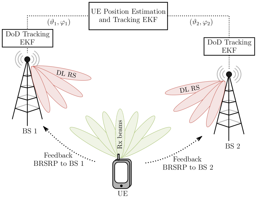
Figure 1: Illustration of the UE positioning approach considered in this paper. In particular, UEs feedback RSRP measurements obtained from DL RSs and transmitted across multiple BS beams. Only angles are used for positioning purposes. A single BS suffices in determining the $2$D position of a UE given that its height is known. For $3$D positioning at least two BSs are needed.

III Proposed Extended Kalman Filter

We now consider sequential estimation of the UE’s $3$D position by means of a two-stage EKF. In particular, each BS employs an EKF for estimating and tracking the DoD using feedback BRSRP measurements from the UE. This is the first stage of the sequential estimation procedure. The second stage EKF consists in fusing the DoDs according to their covariance matrices, both tracked by the first stage EKFs, into position estimates. We follow the so-called information form EKF instead of the more widely used Kalman-gain formulation. In fact, the former is computationally more attractive than the latter when the state-vector has smaller dimension than the observation (or measurement) vector. For example, for $\mathcal{M}_{\mathrm{BS}}=64$ beams and $2$ parameters composing the state-vector ($\vartheta,\varphi$) the information-form EKF needs to invert a $2\times 2$ matrix while in the Kalman-gain formulation a $64\times 64$ matrix inversion is required at each step. Note that the two-stage EKF proposed in this section may be understood as an extension of the work in [5] to BRSRP measurements, instead of using relative-phase measurements.

III-A EKF for DoD Estimation and Tracking

The state vector for the DoD-EKF is $\bm{s}=[\vartheta,\varphi,\Delta\vartheta,\Delta\varphi]^{\textrm{T}}$, where $\Delta\vartheta$ and $\Delta\varphi$ denote the rate-of-change of $\vartheta$ and $\varphi$, respectively. The prediction step of the DoD-EKF is then

$$\bm{s}^{-}[n] =\bm{F}\bm{s}^{+}[n-1]$$ (4)

$$\bm{C}^{-}[n] =\bm{F}\bm{C}^{+}[n-1]\bm{F}^{\textrm{T}}+\bm{Q},$$ (5)

where $\bm{F}\in\mathbb{R}^{4\times 4}$, $\bm{C}\in\mathbb{R}^{4\times 4}$, and $\bm{Q}\in\mathbb{R}^{4\times 4}$ denote the state-transition matrix, state covariance matrix, and state-noise covariance matrix, respectively. Matrices $\bm{F}$ and $\bm{Q}$ can be found from [11, Ch.2] by noting that we have employed a continuous white-noise acceleration model for the state-dynamics. The update step of the DoD-EKF is

$$\bm{C}^{+}[n] =\left(\bm{C}^{-}[n]^{-1}+\bm{\mathcal{I}}(\bm{s}^{-}[n])\right)^{-1}$$ (6)

$$\Delta\bm{s}[n] =\bm{C}^{+}[n]\,\bm{q}(\bm{s}^{-}[n])$$ (7)

$$\bm{s}^{+}[n] =\bm{s}^{-}[n]+\Delta\bm{s}[n],$$ (8)

where $\bm{\mathcal{I}}(\bm{s}^{-}[n])\in\mathbb{R}^{4\times 4}$ and $\bm{q}(\bm{s}^{-}[n])\in\mathbb{R}^{4}$ denote the observed Fisher information matrix (FIM) and gradient of the log-likelihood function of the state given BRSRP measurements, respectively.

In particular, BRSRP measurements can be shown to follow a noncentral $\chi^{2}$-distribution with a probability density function (pdf) given by [6],[12, Ch.2]

$$\begin{split}p(\beta_{i,j})=&\frac{\mathcal{M}_{f}}{\tilde{\sigma}_{i,j}^{2}}\left(\frac{\mathcal{M}_{f}\beta_{i,j}}{\lambda_{i,j}}\right)^{\frac{\mathcal{M}_{f}-1}{2}}\textrm{e}^{-\frac{\lambda_{i,j}+\mathcal{M}_{f}\beta_{i,j}}{\tilde{\sigma}_{i,j}^{2}}}\\ &\times I_{\mathcal{M}_{f}-1}\left(\frac{2\sqrt{\lambda_{i,j}\mathcal{M}_{f}\beta_{i,j}}}{\tilde{\sigma}_{i,j}^{2}}\right),\end{split}$$ (9)

where $I_{x}(\cdot)\in\mathbb{R}$ denotes a modified Bessel function of the first kind. For a growing number of subcarriers $\mathcal{M}_{f}$, the pdf in (9) approaches a Gaussian [6], and we thus have

$$\beta_{i,j}\sim\mathcal{N}(\mu_{i,j},\sigma_{i,j}^{2}).$$ (10)

Here, the mean and variance of BRSRP measurements are given, respectively, by

$$\mu_{i,j} =\frac{\lambda_{i,j}}{\mathcal{M}_{f}}+\tilde{\sigma}_{i,j}^{2}$$ (11)

$$\sigma_{i,j}^{2} =\frac{\tilde{\sigma}_{i,j}^{4}}{\mathcal{M}_{f}}+\frac{2\tilde{\sigma}_{i,j}^{2}\lambda_{i,j}}{\mathcal{M}_{f}^{2}},$$ (12)

where

$$\lambda_{i,j} =\sum_{m=1}^{\mathcal{M}_{f}}|[\bm{S}]_{m}[\bm{b}_{f}]_{m}\gamma_{i,j}|^{2}$$ (13)

$$\gamma_{i,j} =\bm{b}_{\mathrm{UE}}^{i\,\textrm{T}}(\vartheta_{a},\varphi_{a})\bm{\Gamma}\bm{b}_{\mathrm{BS}}^{j}(\vartheta_{d},\varphi_{d}).$$ (14)

Let $\bm{\beta}\in\mathbb{R}^{\mathcal{M}_{\mathrm{BS}}}$ denote the BRSRP measurements for all BS beams and a given UE beam. The chosen UE beam can be the one that yields the largest sum of BS’s BRSRP measurements among all UE beams, i.e. $\max_{i}\sum_{j=1}^{\mathcal{M}_{\mathrm{BS}}}\beta_{i,j}$, or simply the UE beam corresponding to the largest BRSRP measurement, for example. It follows that $\bm{\beta}\sim\mathcal{N}(\bm{\mu}(\bm{\Theta}),\bm{C}(\bm{\Theta}))$, where

$$\bm{\mu}(\bm{\Theta}) =\bm{A}(\vartheta_{d},\varphi_{d})\bm{\alpha}\frac{P_{\mathrm{Tx}}}{\mathcal{M}_{f}}+\bm{1}\tilde{\sigma}^{2}$$ (15)

$$\bm{C}(\bm{\Theta}) =\mathrm{diag}\left\{\bm{A}(\vartheta_{d},\varphi_{d})\bm{\alpha}\frac{2\tilde{\sigma}^{2}P_{\mathrm{Tx}}}{\mathcal{M}_{f}^{2}}+\bm{1}\frac{\tilde{\sigma}^{4}}{\mathcal{M}_{f}}\right\}.$$ (16)

Here, $\bm{\Theta}=[\vartheta_{d},\varphi_{d},\alpha_{1},\alpha_{4},\Re\{\alpha_{2}\},\Im\{\alpha_{2}\},\tilde{\sigma}^{2}]^{\textrm{T}}$ denotes the unknown parameter vector and $\bm{\alpha}=[\alpha_{1},\ldots,\alpha_{4}]^{\textrm{T}}$ is given by $\bm{\alpha}=\mathrm{vec}\{\bm{\Gamma}^{H}\bm{b}^{i^{\ast}}_{\mathrm{UE}}(\vartheta_{a},\varphi_{a})\bm{b}^{i\,{\textrm{T}}}_{\mathrm{UE}}(\vartheta_{a},\varphi_{a})\bm{\Gamma}\}$. Moreover, $P_{\mathrm{Tx}}=\sum_{m=1}^{\mathcal{M}_{f}}|[\bm{S}]_{m}[\bm{b}_{f}]_{m}|^{2}$ and $\bm{A}(\vartheta_{d},\varphi_{d})\in\mathbb{C}^{\mathcal{M}_{\mathrm{BS}}\times 4}$ is given by

$$\begin{split}\bm{A}(\vartheta_{d},\varphi_{d})=[&\bm{b}^{\ast}_{\mathrm{BS}_{\phi}}(\vartheta_{d},\varphi_{d})\odot\bm{b}_{\mathrm{BS}_{\phi}}(\vartheta_{d},\varphi_{d}),\\ &\bm{b}^{\ast}_{\mathrm{BS}_{\theta}}(\vartheta_{d},\varphi_{d})\odot\bm{b}_{\mathrm{BS}_{\phi}}(\vartheta_{d},\varphi_{d}),\\ &\bm{b}^{\ast}_{\mathrm{BS}_{\phi}}(\vartheta_{d},\varphi_{d})\odot\bm{b}_{\mathrm{BS}_{\theta}}(\vartheta_{d},\varphi_{d}),\\ &\bm{b}^{\ast}_{\mathrm{BS}_{\theta}}(\vartheta_{d},\varphi_{d})\odot\bm{b}_{\mathrm{BS}_{\theta}}(\vartheta_{d},\varphi_{d})],\end{split}$$ (17)

where $\odot$ denotes the Hadamard-Schur (element-wise) product.

The EKF can now be implemented with the observed FIM and gradient of the log-likelihood function of $\bm{\Theta}\in\mathbb{R}^{7}$ by exploiting the asymptotic (Gaussian) distribution of BRSRP measurements. Convenient expressions for the FIM and gradient under Gaussian distributed observations can be found in [8, Ch.3]. However, such an approach may not be computationally attractive since one would need to track $7$ parameters out of which only $2$ are of interest for angle based positioning. We would thus need to track $5$ nuisance parameters. Since the computational complexity of each EKF iteration is typically $\mathcal{O}(n^{3})$, where $n$ denotes the dimension of the state-vector, it is important in practice to formulate the sequential estimation problem at hand in a way that only the DoD is tracked at each BS.

Let us thus define the received signal-to-noise ratio (SNR) of the $(i,j)$ beam pair as

$$\mathrm{SNR}_{i,j}\triangleq\frac{\lambda_{i,j}}{\mathcal{M}_{f}\tilde{\sigma}^{2}_{i,j}}.$$ (18)

In the low SNR regime we have $\mathcal{M}_{f}\tilde{\sigma}^{2}_{i,j}>\lambda_{i,j}$. Moreover, the break-even point between both terms composing the variance of BRSRP measurements in (12) is $\mathcal{M}_{f}\tilde{\sigma}^{2}_{i,j}=2\lambda_{i,j}$. Hence, we make a low-SNR approximation of the covariance of $\bm{\beta}$ and assume it is independent of the DoD. The resulting log-likelihood function is

$$\begin{split}\ell_{\mathrm{aprx}}(\bm{\Theta},\sigma^{2}|\bm{\beta})=&-\frac{\mathcal{M}_{\mathrm{BS}}}{2}\ln{2\pi}-\frac{\mathcal{M}_{\mathrm{BS}}}{2}\ln{\sigma^{2}}\\ &-\frac{1}{2\sigma^{2}}\|\bm{\beta}-\bm{\mu}(\bm{\Theta}))\|^{2}.\end{split}$$ (19)

The above log-likelihood function is separable in $(\vartheta_{d},\varphi_{d})$ and $(\bm{\alpha},\tilde{\sigma}^{2},\sigma^{2})$ since the maximum likelihood estimator (MLE) of the latter parameters may be found in a closed-form for a given $(\vartheta,\varphi)$ [13, 14]. Hence, the concentrated log-likelihood function is

$$\begin{split}\ell_{\mathrm{caprx}}(\vartheta_{d},\varphi_{d}|\bm{\beta})=&-\frac{\mathcal{M}_{\mathrm{BS}}}{2}\ln 2\pi-\frac{\mathcal{M}_{\mathrm{BS}}}{2}\\ &-\frac{\mathcal{M}_{\mathrm{BS}}}{2}\ln\frac{\|\bm{P}^{\bot}_{A1}(\vartheta_{d},\varphi_{d})\bm{\beta}\|^{2}}{\mathcal{M}_{\mathrm{BS}}}.\end{split}$$ (20)

Such an expression is obtained by replacing $\bm{\alpha}$ and $\sigma^{2}$ in (19) with the corresponding MLEs:

$$\begin{split}\begin{bmatrix}\hat{\bm{\alpha}}\\ \hat{\tilde{\sigma}}^{2}\end{bmatrix}&=\left[\bm{A}(\vartheta_{d},\varphi_{d})\frac{P_{\mathrm{Tx}}}{\mathcal{M}_{f}},\,\bm{1}\right]^{\dagger}\bm{\beta}\\ \hat{\sigma}^{2}&=\frac{1}{\mathcal{M}_{\mathrm{BS}}}\|\bm{P}^{\bot}_{A1}(\vartheta_{d},\varphi_{d})\bm{\beta}\|^{2}.\end{split}$$ (21)

Here, $(\cdot)^{\dagger}$ denotes the Moore-Penrose pseudo-inverse. Moreover, $\bm{P}^{\bot}_{A1}(\vartheta_{d},\varphi_{d})=\bm{I}-\bm{P}_{A1}(\vartheta_{d},\varphi_{d})$, and $\bm{P}_{A1}(\vartheta_{d},\varphi_{d})\in\mathbb{R}^{\mathcal{M}_{\mathrm{BS}}\times\mathcal{M}_{\mathrm{BS}}}$ denotes an orthogonal projection matrix. We note that $\bm{P}_{A1}(\vartheta_{d},\varphi_{d})=\bm{\mathcal{P}}_{A}(\vartheta_{d},\varphi_{d})+\bm{\mathcal{P}}_{1}$, where $\bm{\mathcal{P}}_{A}(\vartheta_{d},\varphi_{d})$ and $\bm{\mathcal{P}}_{1}$ denote oblique projection matrices. In particular, the range-space of $\bm{\mathcal{P}}_{A}(\vartheta_{d},\varphi_{d})$ is spanned by the columns of $\bm{A}(\vartheta_{d},\varphi_{d})$ while its nullspace contains a subspace spanned by vector $\bm{1}$. Similarly, the range-space of $\bm{\mathcal{P}}_{1}$ is spanned by vector $\bm{1}$ while its nullspace contains a subspace spanned by the columns of $\bm{A}(\vartheta_{d},\varphi_{d})$ [15].

The gradient and observed FIM (or Hessian) of the concentrated log-likelihood function now follows from the results in [16, 17]

$$[\bm{q}(\vartheta_{d},\varphi_{d})]_{1} =2\left(\frac{\partial}{\partial\vartheta_{d}}\bm{P}^{\bot}_{A1}(\vartheta_{d},\varphi_{d})\,\bm{\beta}\right)^{\textrm{T}}\bm{P}^{\bot}_{A1}(\vartheta_{d},\varphi_{d})\,\bm{\beta}$$ (22)

$$[\bm{q}(\vartheta_{d},\varphi_{d})]_{2} =2\left(\frac{\partial}{\partial\varphi_{d}}\bm{P}^{\bot}_{A1}(\vartheta_{d},\varphi_{d})\,\bm{\beta}\right)^{\textrm{T}}\bm{P}^{\bot}_{A1}(\vartheta_{d},\varphi_{d})\,\bm{\beta}$$ (23)

$$[\bm{\mathcal{I}}(\vartheta_{d},\varphi_{d})]_{1,2} \approx 2\left(\frac{\partial}{\partial\vartheta_{d}}\bm{P}^{\bot}_{A1}(\vartheta_{d},\varphi_{d})\,\bm{\beta}\right)^{\textrm{T}}$$

$$\hskip 56.9055pt\times\frac{\partial}{\partial\varphi_{d}}\bm{P}^{\bot}_{A1}(\vartheta_{d},\varphi_{d})\,\bm{\beta}.$$ (24)

Note that we have used a first-order approximation of the observed FIM since it is known to provide improved convergence [17]. The proposed EKF for DoD employs the above gradient and observed FIM in the update-step. Next, the DoDs and corresponding covariance matrices tracked by the DoD-EKF are used for tracking the UE position.

III-B EKF for UE Positioning

The DoD estimates tracked by the EKF proposed in the previous section can be assumed to be given by

$$\begin{bmatrix}\hat{\vartheta}_{k}\\ \hat{\varphi}_{k}\end{bmatrix}\sim\mathcal{N}\left(\begin{bmatrix}\vartheta_{k}\\ \varphi_{k}\end{bmatrix},\bm{C}_{k}\right),$$ (25)

where the subscript $k$ denotes the BS index. Note that the covariance $\bm{C}_{k}\in\mathbb{R}^{2\times 2}$ equals the upper-left $(2\times 2)$ block of $\bm{C}^{+}[n]$ in the DoD-EKF, and it is assumed to be angle-independent. Such a simplifying assumption is taken here since a closed-form expression for $\bm{C}_{k}$ is typically rather involved, which in turn would significantly increase the complexity of the Pos-EKF proposed in this section. In particular, let the state vector be given by $\bm{s}_{\mathrm{UE}}=[x_{\mathrm{UE}},y_{\mathrm{UE}},z_{\mathrm{UE}},v_{x},v_{y},v_{z}]^{\textrm{T}}$. The prediction step of the Pos-EKF is then

$$\bm{s}_{\mathrm{UE}}^{-}[n] =\bm{F}_{\mathrm{UE}}\bm{s}_{\mathrm{UE}}^{+}[n-1]$$ (26)

$$\bm{C}^{-}_{\mathrm{UE}}[n] =\bm{F}_{\mathrm{UE}}\bm{C}_{\mathrm{UE}}^{+}[n-1]\bm{F}^{\textrm{T}}_{\mathrm{UE}}+\bm{Q}_{\mathrm{UE}},$$ (27)

where $\bm{F}_{\mathrm{UE}}\in\mathbb{R}^{6\times 6}$, $\bm{C}_{\mathrm{UE}}\in\mathbb{R}^{6\times 6}$, and $\bm{Q}_{\mathrm{UE}}\in\mathbb{R}^{6\times 6}$ denote the state-transition matrix, state covariance matrix, and state-noise covariance matrix, respectively. Similarly to the DoD-EKF, matrices $\bm{F}_{\mathrm{UE}}$ and $\bm{Q}_{\mathrm{UE}}$ can be found from [11, Ch.2] by noting that we have employed a continuous white-noise acceleration model for the UE state-dynamics. The update step of the Pos-EKF is

$$\bm{C}^{+}_{\mathrm{UE}}[n] =\left(\bm{C}^{-}_{\mathrm{UE}}[n]^{-1}+\bm{\mathcal{I}}_{\mathrm{UE}}(\bm{s}^{-}_{\mathrm{UE}}[n])\right)^{-1}$$ (28)

$$\Delta\bm{s}_{\mathrm{UE}}[n] =\bm{C}^{+}_{\mathrm{UE}}[n]\,\bm{q}_{\mathrm{UE}}(\bm{s}^{-}_{\mathrm{UE}}[n])$$ (29)

$$\bm{s}^{+}_{\mathrm{UE}}[n] =\bm{s}^{-}_{\mathrm{UE}}[n]+\Delta\bm{s}_{\mathrm{UE}}[n],$$ (30)

where $\bm{\mathcal{I}}_{\mathrm{UE}}(\bm{s}^{-}_{\mathrm{UE}}[n])\in\mathbb{R}^{6\times 6}$ and $\bm{q}_{\mathrm{UE}}(\bm{s}^{-}_{\mathrm{UE}}[n])\in\mathbb{R}^{6}$ denote the observed FIM and gradient of the log-likelihood function of UE position given DoD estimates from multiple BSs.

Let $\bm{m}\in\mathbb{R}^{2K}$ denote the estimated DoDs of $K$ BSs towards a UE. It follows from (25) that $\bm{m}\sim\mathcal{N}\left(\bm{\mu}(\bm{p}),\bm{C}\right)$, where

$$\bm{\mu}(\bm{p}) =\left[\vartheta_{1}(\bm{p}),\varphi_{1}(\bm{p}),\ldots,\vartheta_{K}(\bm{p}),\varphi_{K}(\bm{p})\right]^{\textrm{T}}$$ (31)

$$\bm{C} =\mathrm{blkdiag}\left\{\bm{C}_{1},\ldots,\bm{C}_{K}\right\}.$$ (32)

Here, $\bm{p}\in\mathbb{R}^{3}$ denotes the $3$D Cartesian coordinate of a UE’s position and $\mathrm{blkdiag}\{\cdot\}$ denotes a block-diagonal matrix. Note that

$$\vartheta_{k}(\bm{p}) =\arctan\left(\frac{-\Delta z_{k}}{d_{{2D}_{k}}}\right)+\pi/2$$ (33)

$$\varphi_{k}(\bm{p}) =\arctan 2\left(\Delta y_{k},\Delta x_{k}\right),$$ (34)

where $d_{{2D}_{k}}=\sqrt{\Delta x^{2}_{k}+\Delta y^{2}_{k}}$, $\Delta x_{k}=x_{\mathrm{UE}}-x_{\mathrm{BS}_{k}}$, $\Delta y_{k}=y_{\mathrm{UE}}-y_{\mathrm{BS}_{k}}$, and $\Delta z_{k}=z_{\mathrm{UE}}-z_{\mathrm{BS}_{k}}$. The gradient of the log-likelihood function of $\bm{p}$ given $\bm{m}$, and respective observed FIM, now follow from [8, Ch.3]

$$[\bm{q}_{\mathrm{UE}}(\bm{p})]_{m} =\left(\frac{\partial\bm{\mu}(\bm{p})}{\partial[\bm{p}]_{m}}\right)^{\textrm{T}}\bm{C}^{-1}\left(\bm{m}-\bm{\mu}(\bm{p})\right)$$ (35)

$$[\bm{\mathcal{I}}_{\mathrm{UE}}(\bm{p})]_{m,n} \approx\left(\frac{\partial\bm{\mu}(\bm{p})}{\partial[\bm{p}]_{m}}\right)^{\textrm{T}}\bm{C}^{-1}\frac{\partial\bm{\mu}(\bm{p})}{\partial[\bm{p}]_{n}}.$$ (36)

IV Numerical Results

IV-A Deployment Scenario

We consider a scenario where two BSs and a UE are deployed on the Madrid grid. In particular, a modification to the original Madrid grid is considered in this paper in order to obtain a large (up to $500\text{\,}\mathrm{m}$ long) open area. This is a common envisioned deployment for mmW cellular systems. Fig. 2 illustrates the modified Madrid grid considered in here as well as the locations of the BSs and UE. In particular, BSs are deployed at a height of $50\text{\,}\mathrm{m}$ while that of the UE is $1.5\text{\,}\mathrm{m}$.

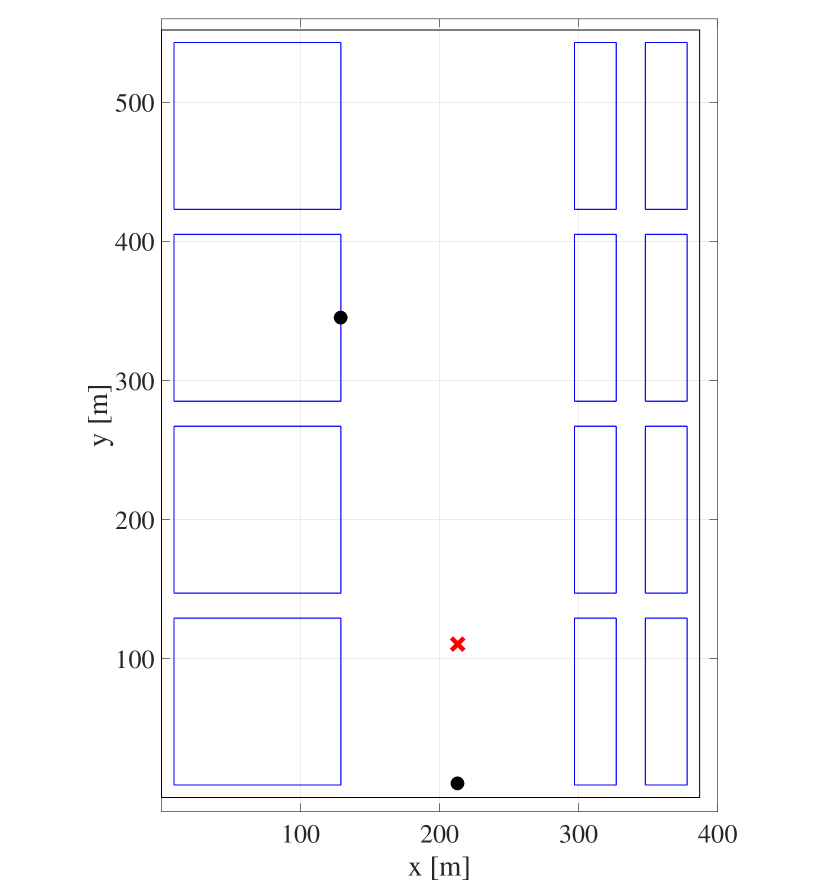
Figure 2: Illustration of the deployment scenario considered in this paper for assessing the performance of the proposed $2$-stage EKF. We have modified the Madrid grid in order to have a larger open area between BSs (black dots) and UE (red cross). The radio channel between UE and BSs is according to the METIS ray-tracing channel model [18].

The mmW system considered in this numerical study operates at $39\text{\,}\mathrm{GHz}$ with a bandwidth of $200\text{\,}\mathrm{MHz}$ and subcarrier spacing of $120\text{\,}\mathrm{kHz}$. The number of subcarriers available for transmitting DL-RSs is $1656$. The power budget at each BS is $21\text{\,}\mathrm{d}\mathrm{B}\mathrm{m}$. Each BS transmits DL-RSs through $64$ beams pointing in different directions. In particular, such BS beams span $40^{\circ}$ both in elevation and azimuth, and the $3\text{\,}\mathrm{dB}$ beamwidth is $\approx 3^{\circ}$. DL-RSs for different beams and BSs are assumed to be scheduled in orthogonal radio resources. The UE receives DL-RSs from $52$ beams spanning $360^{\circ}$ in azimuth and a fixed direction ($\approx 75^{\circ}$) in co-elevation. The $3\text{\,}\mathrm{dB}$ beamwidth is $\approx 6^{\circ}$ in azimuth and $\approx 40^{\circ}$ in elevation. The maximum gains of the BS and UE beams are $\approx 30\text{\,}\mathrm{d}\mathrm{B}\mathrm{i}$ and $\approx 17\text{\,}\mathrm{d}\mathrm{B}\mathrm{i}$, respectively. The UE measures the BRSRP for all $64\times 52$ beam-pairs, for both BSs, in $160\text{\,}\mathrm{ms}$, after which it feedbacks the highest BRSRPs. The amount of feedback BRSRPs may be signalled by the network, for example.

The radio channels between a given UE and BSs are modelled according to the METIS ray-tracing channel model [18]. Hence, all multipath components between the UE and BSs are taken into account in the BRSRPs measurements, and re-calculated for every UE position.

IV-B Performance of the Proposed EKF

We assess the performance of the proposed two-stage EKF by considering a UE moving with a velocity of $2\text{\,}\mathrm{m}\text{\,}{\mathrm{s}}^{-1}$. The UE moves along a $100\text{\,}\mathrm{m}$-long straight trajectory with a south-to-north direction. The starting position of the UE is illustrated in Fig. 2. The southernmost BS is north-facing while the northernmost BS has a $60\text{\,}\mathrm{\SIUnitSymbolDegree}$ orientation clockwise from East-side. The UE feedbacks BRSRP measurements every $160\text{\,}\mathrm{ms}$. Initialization of the DoD-EKF and Pos-EKF follows that in [5].

In particular, we consider the case when the number of feedback BRSRP measurements (corresponding to beam-pairs) is $16$, $8$, $6$, and $5$. For less than five BRSRP measurements the corresponding angle-domain ambiguity function is far from the ideal Dirac-delta, and the resulting likelihood function has multiple global maxima. Hence, the performance of the proposed EKF degrades rapidly when the number of feedback BRSRP measurements is smaller than five. We emphasize that the performance of the proposed EKF with respect to the number of feedback BRSRP measurements is heavily dependent on the shape of the BSs’ transmit beams. Therefore, one can achieve sub-meter $3$D positioning accuracy with, say, three BRSRP measurements given that the BSs’ transmit beams have the necessary characteristics in terms of angle-domain ambiguity function.

The performance metrics employed to assess the performance of the proposed EKF are the 3D positioning error $(\sqrt{\tilde{x}^{2}+\tilde{y}^{2}+\tilde{z}^{2}})$, elevation angle error $(|\tilde{\vartheta}|)$ as well as azimuth angle error $(|\tilde{\varphi}|)$. The corresponding cumulative distribution functions (CDFs) are illustrated in Figs. 3-5. The CDF of the received SNR per beam is also given in Fig. 6. Results show that reporting the five beams (out of the available $64$ beams) corresponding to the highest BRSRP measurements suffices in achieving sub-meter $3$D positioning accuracy in $90\text{\,}\mathrm{\char 37\relax}$ of the UE’s trajectory. Also, increasing the number of feedback beams improves the positioning accuracy only slightly. This may be understood by the high directivity of the employed transmit beams. In particular, reporting RSRP measurements of beams that have a main-lobe towards directions away from the LoS between BS and UE leads to a marginal increase (and may even be detrimental for low-SNR) in angle-related information compared to the beams that point towards the UE. In practice, this is important since it allows one to optimize the capacity of the feedback channel.

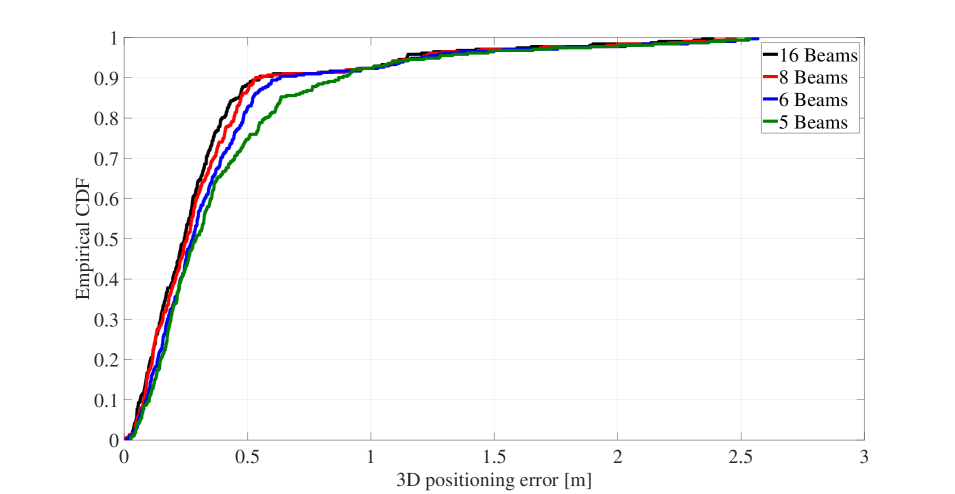
Figure 3: Empirical CDF of $3$D positioning error obtained using the proposed EKF for a varying number of feedback BRSRP measurements. Reporting the five beams (out of the available $64$ beams) corresponding to the highest BRSRP measurements suffices in achieving sub-meter $3$D positioning accuracy in $90\text{\,}\mathrm{\char 37\relax}$ of the UE’s trajectory. This is due to the high directivity of the employed transmit beams and allows one to optimize the capacity of the feedback channel.

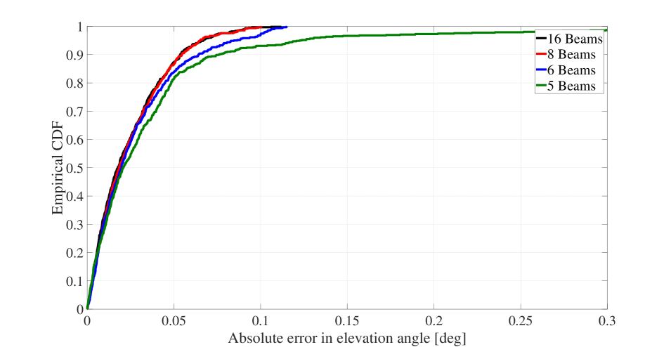
Figure 4: Empirical CDF of elevation-angle error obtained using the proposed EKF for a varying number of feedback BRSRP measurements. Increasing the number of feedback beams improves the accuracy only slightly. This is due to the high directivity of the employed transmit beams.

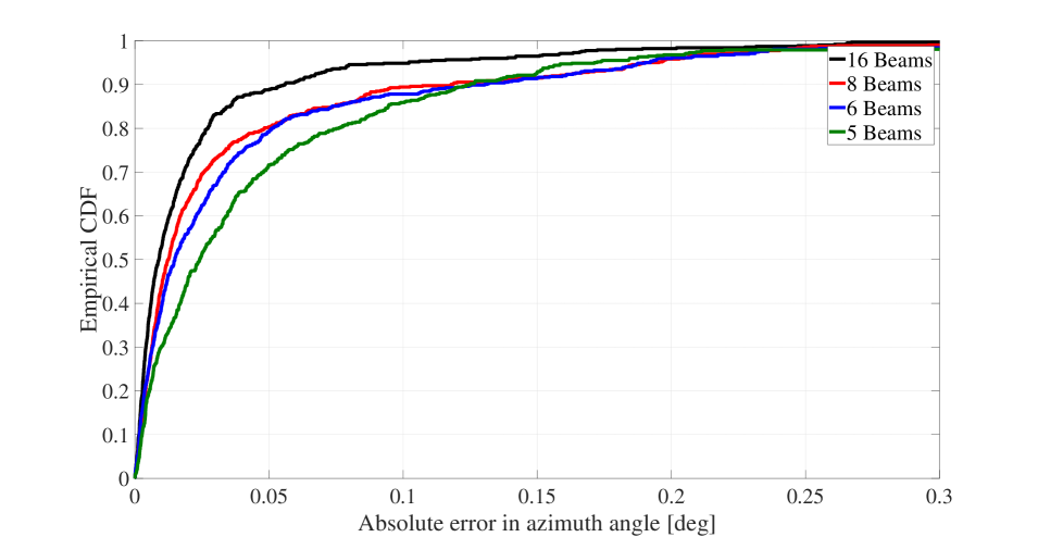
Figure 5: Empirical CDF of azimuth-angle error obtained using the proposed EKF for a varying number of feedback BRSRP measurements. Increasing the number of feedback beams improves the accuracy only slightly. This is due to the high directivity of the employed transmit beams.

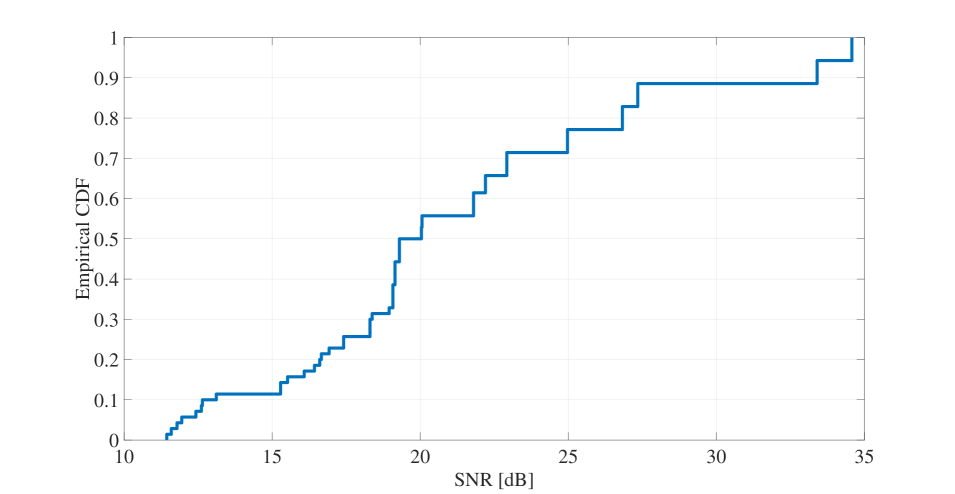
Figure 6: Empirical CDF of received SNR at the UE, after gain from transmit/receive beams, for the $16$ beams considered for reporting.

V Conclusion

In this article, we proposed a 3D UE positioning method for 5G mmW networks by exploiting $3$D downlink beamforming from base-stations. More specifically, the proposed sequential 3D UE position estimation was performed at the network-side by means of a two-stage EKF and based on feedback beam-RSRP measurements carried out at the UE. In particular, in the first EKF stage, the directions-of-departure of the beamformed DL RSs in the feedback scheme were estimated and tracked at BSs, whereas in the second angle-based EKF stage, such angle estimates were fused from all available BSs into 3D position estimates at a central entity. Performance results of the proposed algorithm on a realistic outdoor 5G deployment based on the METIS ray-tracing propagation model show that sub-meter $3$D positioning accuracy of users is achievable in 90% of the cases by reporting only $8$ base-station DL beams.

Future work includes taking into account uncertainties in BSs’ orientation for UE positioning.

References

- [1] 3GPP, TR22.872, “Study on positioning use cases, stage 1,” 2016. [Online]. Available: https://portal.3gpp.org/desktopmodules/Specifications/SpecificationDetails.aspx?specificationId=3280
- [2] 3GPP, RP-172746, “New SID: study on NR positioning support,” 2017. [Online]. Available: https://portal.3gpp.org/ngppapp/CreateTdoc.aspx?mode=view&contributionId=853821
- [3] S. Sun, T. S. Rappaport, R. W. Heath, A. Nix, and S. Rangan, “MIMO for millimeter-wave wireless communications: beamforming, spatial multiplexing, or both?” IEEE Comm. Magazine, vol. 52, no. 12, pp. 110–121, December 2014.
- [4] 3GPP, TS38.214, “Physical layer procedures for data,” 2018. [Online]. Available: https://portal.3gpp.org/desktopmodules/Specifications/SpecificationDetails.aspx?specificationId=3216
- [5] M. Koivisto, M. Costa, J. Werner, K. Heiska, J. Talvitie, K. Leppänen, V. Koivunen, and M. Valkama, “Joint Device Positioning and Clock Synchronization in 5G Ultra-Dense Networks,” IEEE Trans. Wireless Comm., vol. 16, no. 5, pp. 2866–2881, May 2017.
- [6] R. Pohlmann, S. Zhang, T. Jost, and A. Dammann, “Power-based direction-of-arrival estimation using a single multi-mode antenna,” in 2017 14th Workshop on Positioning, Navigation and Communications (WPNC), Oct 2017, pp. 1–6.
- [7] J. P. Lie, T. Blu, and C. M. S. See, “Single antenna power measurements based direction finding,” IEEE Trans. Signal Proc., vol. 58, no. 11, pp. 5682–5692, Nov 2010.
- [8] S. Kay, Fundamentals of Statistical Signal Processing: Estimation Theory. Prentice-Hall Signal Processing Series, 1993.
- [9] A. Molisch, “A generic model for MIMO wireless propagation channels in macro- and microcells,” IEEE Trans. Signal Proc., vol. 52, no. 1, pp. 61–71, Jan 2004.
- [10] A. Richter, “Estimation of radio channel parameters: Models and algorithms,” Ph.D. dissertation, Technische Universität Ilmenau, 2005, http://www.db-thueringen.de/servlets/DerivateServlet/Derivate-7407/ilm1-2005000111.pdf.
- [11] J. Hartikainen, A. Solin, and S. Särkkä, “Optimal filtering with Kalman filters and smoothers,” Aug 2011. [Online]. Available: http://becs.aalto.fi/en/research/bayes/ekfukf/documentation.pdf
- [12] J. Proakis and M. Salehi, Digital Communications, 5th ed. McGraw-Hill, 2008.
- [13] G. Golub and V. Pereyra, “Separable nonlinear least squares: the variable projection method and its applications,” Inverse Problems, vol. 19, no. 2, p. R1, 2003.
- [14] B. Ottersten, M. Viberg, and T. Kailath, “Analysis of subspace fitting and ML techniques for parameter estimation from sensor array data,” IEEE Trans. Signal Proc., vol. 40, no. 3, pp. 590–600, Mar 1992.
- [15] R. Behrens and L. Scharf, “Signal processing applications of oblique projection operators,” IEEE Trans. Signal Proc., vol. 42, no. 6, pp. 1413–1424, Jun 1994.
- [16] P. Stoica and A. Nehorai, “MUSIC, Maximum Likelihood, and Cramér-Rao bound: further results and comparisons,” IEEE Trans. Acoust., Speech, and Signal Proc., vol. 38, no. 12, pp. 2140–2150, Dec 1990.
- [17] M. Viberg, B. Ottersten, and T. Kailath, “Detection and estimation in sensor arrays using weighted subspace fitting,” IEEE Trans. Signal Proc., vol. 39, no. 11, pp. 2436–2449, Nov 1991.
- [18] METIS, “D1.4 Channel models,” Feb. 2015. [Online]. Available: https://www.metis2020.com/wp-content/uploads/METIS_D1.4_v3.pdf