Theoretical spin-wave dispersions in the antiferromagnetic phase AF1 of MnWO₄ based on the polar atomistic model in P2

Abstract

The spin wave dispersions of the low temperature antiferromagnetic phase (AF1) MnWO₄ have been numerically calculated based on the recently reported non-collinear spin configuration with two different canting angles. A Heisenberg model with competing magnetic exchange couplings and single-ion anisotropy terms could properly describe the spin wave excitations, including the newly observed low-lying energy excitation mode $\omega_{2}$=0.45 meV appearing at the magnetic zone centre. The spin wave dispersion and intensities are highly sensitive to two differently aligned spin-canting sublattices in the AF1 model. Thus this study reinsures the otherwise hardly provable hidden polar character in MnWO₄.

I I. INTRODUCTION

Multiferroic properties, which show ferroelectricity or ferroelasticity coexisting with magnetic order, have attracted great attention both experimentally and theoretically. Of particular interest for such materials is that they may have potential applications in electronic devices like magnetoelectric sensors and data storage chips M.Maczka2012 . A number of materials such as $R$MnO₃ ($R$ is rare earth element) T.Kimura2003 ; T.Goto2004 , $R$Mn₂O₅ N.Hur2004 ; D.Higashiyama2005 , CoCr₂O₄ Y.Yamasaki2006 exhibiting a strong interplay between the magnetic and ferroelectric order have been intensively studied. Several different models have been proposed to explain the mechanism of magnetoelectric effects H.Katsura2005 ; I.A.Sergienko2006 ; M.Mostovoy2006 ; A.B.Harris2007 ; T.Arima2007 . For examples, the change of the modulation wavelength seems to play an important role L.C.Chapon2006 , another key factor can be a noncollinear spin configuration M.Kenzelmann2005 ; T.Arima2006 which is in accord with the theory associated with the Aharonov-Casher effect Y.Aharonov1984 or the inverse Dzyaloshinskii-Moriya (DM) interaction I.A.Sergienko2006 .

Another well-known material is the mineral huebnerite MnWO₄, an exemplary prototype of magnetoelectric control. It is also a promising system for the study of magnetic phase transitions and related critical phenomena, since it exhibits rich magnetic phase diagram by chemical substitutions K.Taniguchi2006 ; A.H.Arkenbout2006 and by applying magnetic fields H.Mitamura2012 . At zero field, three successive antiferromagnetic phase transitions are observed: the commensurate magnetic structure AF1 with propagation vector $\mathbf{k}=(\pm\frac{1}{4},\frac{1}{2},\frac{1}{2})$ is present below 8 K, the incommensurate elliptical spiral spin structure AF2 existing in 8 $\sim$ 12.3 K induces ferroelectric order, and the incommensurate collinear sinusoidal spin structure AF3 is only observed in a narrow temperature range below 13.5 K A.H.Arkenbout2006 ; H.Dachs1969 ; G.Lautenschlaeger1993 . The fundamental crystal structure of MnWO₄ is monoclinic, and the corresponding space group has been believed to be $\emph{{P}}2/c$ until our structural studies confirmed the true symmetry $\emph{{P}}2$ S.H.Park2015 ; U.Gattermann2016-1 ; U.Gattermann2016-2 ; S.H.Park2018 and the two different spin-canting configurations at two Mn²⁺ sublattices, as a symmetrical consequence of the direct polar subgroup relation between $\emph{{P}}2$ and $\emph{{P}}2/c$. This non-collinear spin-canting texture in AF1 of MnWO₄ is in contrast to the previous collinear magnetic model ($\uparrow\uparrow\downarrow\downarrow$) where the magnetic moments at two Mn sites are aligned collinearly along the easy axis with a common angle of 35^∘-37^∘ against $a$-axis on the (a-c) plane A.H.Arkenbout2006 ; H.Dachs1969 ; G.Lautenschlaeger1993 . With this non-collinear magnetic model, it is necessary to re-examine the excitation spectra as well as the corresponding exchange coupling interactions in the AF1 MnWO₄ as they are sensitive to the spin configurations.

It is known that MnWO₄ is a frustrated magnet with competing exchange interactions G.Lautenschlaeger1993 ; H.Ehrenberg1999 . The analysis of the magnetic excitations allows to explore and clarify the underlying magnetic interactions which dominate the complex spin configurations. There have been several theoretical and experimental investigations H.Ehrenberg1999 ; H.Ehrenberg1996 ; Ye2011 ; Xiao2016 ; Tian2009 on spin wave dispersions in AF1 based on the centrosymmetric space group P2/$c$, where 9$\sim$12 exchange coupling parameters as well as single-ion anisotropy parameter are evaluated within a Heisenberg model. Among these work, in the recent high-resolution inelastic neutron scattering (INS) study of AF1 phase MnWO₄, Xiao et al. Xiao2016 revealed two new electromagnon branches appearing at low energies of $\omega_{1}$=0.07 meV and $\omega_{2}$=0.45 meV at the zone centre, which may reflect the dynamical magnetoelectric coupling and cannot be described by the Heisenberg model.

In this work, we present spin wave calculations based on the polar structure of MnWO₄ (space group $\emph{{P}}2$) as well as the non-collinear magnetic structure, demonstrating that the spin wave dispersion in AF1 can be described by a Heisenberg model with 11 magnetic exchange coupling parameters and single-ion anisotropy. The calculated spectra are visualized in a proper way for easy comparison with previous experimental INS data. Interestingly, one of the electromagnon excitation modes previously denoted as $\omega_{2}$ may be properly described in this study.

II II. Theoretical calculations of spin wave dispersion

As aforementioned, the most recent study S.H.Park2018 showed that MnWO₄ crystallises in monoclinic $\emph{{P}}2$ structure, and the low temperature magnetic structure is not a collinear spin configuration but two spin-canting textures, as illustrated in Fig. 1. The magnetic spins lie in ($a$-$c$) plane with the Mn_a spin-canted about $\theta_{1}=33^{\circ}$ from the $a$-axis while Mn_b about $\theta_{2}=59^{\circ}$.

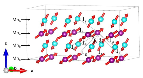
Figure 1: (Color online) The magnetic structure of the AF1 phase of MnWO₄, showing the magnetic Mn²⁺ ions only. Two different spin-canting textures are indicated by the directions of magnetic moments (arrows) of Mn²⁺ ions at both unique sites at Mn_a (in pink) and Mn_b (in cyan blue). Eleven exchange coupling constants $J_{1}$ to $J_{11}$ (dashed lines) are used to fit spin wave dispersions in this study.

The spin wave dispersion curves can be modeled by an effective Heisenberg Hamiltonian

$$H=-\frac{1}{2}\sum_{i,l}{J_{i,l}\mathbf{S}_{i}\cdot\mathbf{S}_{l}}-D_{a}\sum_{i}{(\mathbf{a}\cdot\mathbf{S}_{i})^{2}}-D_{c}\sum_{i}{(\mathbf{c}\cdot\mathbf{S}_{i})^{2}},$$ (1)

where $J_{i,l}$ denotes exchange coupling constants (from $J_{1}$ to $J_{11}$), $D_{a(c)}$ denotes single-ion anisotropy constant.

It should be noted that, for each point occupied by a magnetic atom, an individual axis of quantization is introduced, and with each point $i(l)$ associate a local coordinate system ($x$, $y$, $z$) so that the $z$ axis in this system coincides with the equilibrium spin direction at this point Y.A.Izyumov1970 . For example, the transformation of the vector $\mathbf{S}_{1}$ from the general system of coordinates ($x^{\prime}$, $y^{\prime}$, $z^{\prime}$) associated with the crystallographic axes to the local coordinate system is

$$S_{1}^{x^{\prime}}=S_{1}^{x}\sin{\theta_{1}}+S_{1}^{z}\cos{\theta_{1}},$$

$$S_{1}^{y^{\prime}}=S_{1}^{y},$$

$$S_{1}^{z^{\prime}}=S_{1}^{z}\sin{\theta_{1}}-S_{1}^{x}\cos{\theta_{1}}.$$

Introducing the notation $i$ for spin up ($\uparrow$) sites and $l$ for spin down ($\downarrow$) sites, the linearized Holstein-Primakoff transformation for the quantum spin $\mathbf{S}$ at each site T.Holstein1940 can be written as

$$S_{i,l}^{\dagger}=S_{i,l}^{x}+iS_{i,l}^{y},S_{i,l}^{-}=S_{i,l}^{x}-iS_{i,l}^{y},$$ (2)

and

$$S_{i}^{\dagger}=\sqrt{2S}\bigg{(}1-\frac{a_{i}^{\dagger}a_{i}}{2S}\bigg{)}^{1/2}a_{i}\approx\sqrt{2S}a_{i},$$ (3)

$$S_{i}^{-}=\sqrt{2S}\bigg{(}1-\frac{a_{i}^{\dagger}a_{i}}{2S}\bigg{)}^{1/2}a_{i}^{\dagger}\approx\sqrt{2S}a_{i}^{\dagger},$$ (4)

$$S_{i}^{z}=S-a_{i}^{\dagger}a_{i},$$ (5)

$$S_{l}^{\dagger}=\sqrt{2S}\bigg{(}1-\frac{b_{l}^{\dagger}b_{l}}{2S}\bigg{)}^{1/2}b_{l}^{\dagger}\approx\sqrt{2S}b_{l}^{\dagger},$$ (6)

$$S_{l}^{-}=\sqrt{2S}\bigg{(}1-\frac{b_{l}^{\dagger}b_{l}}{2S}\bigg{)}^{1/2}b_{l}\approx\sqrt{2S}b_{l},$$ (7)

$$S_{l}^{z}=-S+b_{l}^{\dagger}b_{l}.$$ (8)

The Fourier transformation is introduced by:

$$a_{i}^{\dagger}=\sqrt{\frac{1}{N}}\sum_{\mathbf{q}}{\exp{(-i\mathbf{q}\cdot\mathbf{r}_{i})}a_{\mathbf{q}}^{\dagger}},$$ (9)

$$a_{i}=\sqrt{\frac{1}{N}}\sum_{\mathbf{q}}{\exp{(i\mathbf{q}\cdot\mathbf{r}_{i})}a_{\mathbf{q}}},$$ (10)

$$b_{l}^{\dagger}=\sqrt{\frac{1}{N}}\sum_{\mathbf{q}}{\exp{(-i\mathbf{q}\cdot\mathbf{r}_{l})}b_{\mathbf{q}}^{\dagger}},$$ (11)

$$b_{l}=\sqrt{\frac{1}{N}}\sum_{\mathbf{q}}{\exp{(i\mathbf{q}\cdot\mathbf{r}_{l})}b_{\mathbf{q}}}.$$ (12)

Thus, one can obtain the bosonic Hamiltonian in the momentum space as

$$H=-\frac{1}{2}\sum_{q}{\mathbf{a}^{\dagger}H_{q}\mathbf{a}},$$ (13)

with $\mathbf{a}^{\dagger}$=$[a_{q1}^{\dagger}$, $a_{q2}^{\dagger}$, $a_{q3}^{\dagger}$, $a_{q4}^{\dagger}$, $a_{-q1}$, $a_{-q2}$, $a_{-q3}$, $a_{-q4}$, $b_{q1}^{\dagger}$, $b_{q2}^{\dagger}$, $b_{q3}^{\dagger}$, $b_{q4}^{\dagger}$, $b_{-q1}$, $b_{-q2}$, $b_{-q3}$, $b_{-q4}]$, and

$$H_{q}=\left(\begin{array}[]{cccc}M_{11}&M_{12}&M_{13}&M_{14}\\ M_{12}&M_{11}&M_{14}&M_{13}\\ M_{13}&M_{14}&M_{11}&M_{12}\\ M_{14}&M_{13}&M_{12}&M_{11}\end{array}\right),$$ (14)

$$M_{11}=\left(\begin{array}[]{cccc}A_{1}&BP_{2}&C&HP_{2}\\ B^{*}P_{2}&A_{2}&H^{*}P_{2}&C^{*}\\ C^{*}&HP_{2}&A_{1}&FP_{2}\\ H^{*}P_{2}&C&F^{*}P_{2}&A_{2}\end{array}\right),$$ (15)

$$M_{12}=\left(\begin{array}[]{cccccccc}A_{3}&BP_{1}&0&HP_{1}\\ B^{*}P_{1}&A_{4}&H^{*}P_{1}&0\\ 0&HP_{1}&A_{3}&FP_{1}\\ H^{*}P_{1}&0&F^{*}P_{1}&A_{4}\end{array}\right),$$ (16)

$$M_{13}=\left(\begin{array}[]{cccc}0&FP_{1}&0&GP_{1}\\ F^{*}P_{1}&0&G^{*}P_{1}&0\\ 0&GP_{1}&0&BP_{1}\\ G^{*}P_{1}&0&B^{*}P_{1}&0\end{array}\right),$$ (17)

$$M_{14}=\left(\begin{array}[]{cccc}E&FP_{2}&C^{*}&GP_{2}\\ F^{*}P_{2}&E&G^{*}P_{2}&C\\ C&GP_{2}&E&BP_{2}\\ G^{*}P_{2}&C^{*}&B^{*}P_{2}&E\end{array}\right),$$ (18)

with

$$A_{1}= 2(S_{1}J_{4}+S_{1}J_{5}+S_{2}J_{6}-S_{2}J_{7}-S_{2}J_{8}$$ (19)

$$+S_{2}J_{9}-S_{1}D_{c}\sin^{2}{\theta_{1}}-S_{1}D_{a}\cos^{2}{\theta_{1}})$$

$$+S_{1}D_{c}\cos^{2}{\theta_{1}}+S_{1}D_{a}\sin^{2}{\theta_{1}},$$

$$A_{2}= 2(S_{2}J_{4}+S_{2}J_{5}+S_{1}J_{6}-S_{1}J_{7}-S_{1}J_{8}$$ (20)

$$+S_{1}J_{9}-S_{2}D_{c}\sin^{2}{\theta_{2}}-S_{2}D_{a}\cos^{2}{\theta_{2}})$$

$$+S_{2}D_{c}\cos^{2}{\theta_{2}}+S_{2}D_{a}\sin^{2}{\theta_{2}},$$

$$A_{3}=\frac{1}{2}S_{1}D_{c}\cos^{2}{\theta_{1}}+\frac{1}{2}S_{1}D_{a}\sin^{2}{\theta_{1}},$$ (21)

$$A_{4}=\frac{1}{2}S_{2}D_{c}\cos^{2}{\theta_{2}}+\frac{1}{2}S_{2}D_{a}\sin^{2}{\theta_{1}},$$ (22)

$$B= J_{1}e^{-2\pi i[2(0.41029-0.59519)q_{y}+0.5q_{z}]}$$ (23)

$$+J_{2}e^{2\pi i[2(0.09519-0.41029)q_{y}+0.5q_{z}]},$$

$$C= S_{1}\big{\{}J_{3}e^{-2\pi iq_{x}}+J_{10}e^{-2\pi i(-q_{x}-q_{z})}$$ (24)

$$+J_{11}e^{-2\pi i(-q_{x}+q_{z})}\big{\}},$$

$$H= J_{7}\big{\{}e^{-2\pi i[-q_{x}+2(0.41029-0.59519)q_{y}+0.5q_{z}]}$$ (25)

$$+e^{-2\pi i[q_{x}+2(0.41029-0.59519)q_{y}-0.5q_{z}]}\big{\}}$$

$$+J_{8}\big{\{}e^{-2\pi i[-q_{x}+2(0.41029-0.09519)q_{y}-0.5q_{z}]}$$

$$+e^{-2\pi i[q_{x}+2(0.41029-0.09519)q_{y}+0.5q_{z}]}\big{\}},$$

$$E=S_{1}[2J_{4}\cos{q_{z}}+2J_{5}\cos{(-q_{y})}],$$ (26)

$$F= J_{2}e^{-2\pi i[2(0.41029-0.09519)q_{y}+0.5q_{z}]}$$ (27)

$$+J_{1}e^{2\pi i[2(0.59519-0.41029)q_{y}+0.5q_{z}]},$$

$$G= J_{6}\big{\{}e^{2\pi i[-q_{x}+2(0.59519-0.41029)q_{y}-0.5q_{z}]}$$ (28)

$$+e^{2\pi i[q_{x}+2(0.59519-0.41029)q_{y}+0.5q_{z}]}\big{\}}$$

$$+J_{9}\big{\{}e^{2\pi i[-q_{x}+2(0.41029-0.59519)q_{y}+0.5q_{z}]}$$

$$+e^{2\pi i[q_{x}+2(0.41029-0.59519)q_{y}-0.5q_{z}]}\big{\}},$$

$$P_{1,2}=\frac{1}{2}\sqrt{S_{1}S_{2}}[\cos{(\theta_{1}-\theta_{2})}\mp 1].$$ (29)

In order to diagonalize the Hamiltonian Eq.(13), it is needed to introduce a transformation matrix $\mathbf{T}$ R.M.White1965 , and $\mathbf{a}=\mathbf{T}\mathbf{\alpha}$ with $\alpha^{\dagger}$=$[\alpha_{q1}^{\dagger}$, $\alpha_{q2}^{\dagger}$, $\alpha_{q3}^{\dagger}$, $\alpha_{q4}^{\dagger}$, $\alpha_{-q1}$, $\alpha_{-q2}$, $\alpha_{-q3}$, $\alpha_{-q4}$, $\beta_{q1}^{\dagger}$, $\beta_{q2}^{\dagger}$, $\beta_{q3}^{\dagger}$, $\beta_{q4}^{\dagger}$, $\beta_{-q1}$, $\beta_{-q2}$, $\beta_{-q3}$, $\beta_{-q4}]$, so that

$$\mathbf{a}^{\dagger}H_{q}\mathbf{a}=\mathbf{\alpha}^{\dagger}\mathbf{T}^{\dagger}H_{q}\mathbf{T}\mathbf{\alpha}=\mathbf{\alpha}^{\dagger}\omega\mathbf{\alpha},$$ (30)

where $\mathbf{\omega}$ is a diagonal matrix and its diagonal elements are eigenvalues of the system. According to Eq.(30), we obtain $H_{q}\mathbf{T}=(\mathbf{T}^{\dagger})^{-1}\omega$. By using the commutator matrix $\mathbf{I}_{1}=diag{\{1,1,1,1,-1,-1,-1,-1,1,1,1,1,-1,-1,-1,-1\}}$, one can numerically obtain the system’s eigenvalues, i.e., the spin wave excitation energies. The transformation matrix $\mathbf{T}$ is a $16\times 16$ matrix with columns that are eigenvectors to $\mathbf{I}_{1}H_{q}\mathbf{T}=\omega\mathbf{T}$, and it also must respect the Bose commutation rules. Once the correct transformation matrix $\mathbf{T}$ is obtained, the differential scattering cross sections for magnetic scattering are calculated S.W.Lovesey1984 ; T.B.S.Jensen ; T.B.S.Jensen2009 , as follows:

$$\frac{d^{2}\sigma}{d\Omega dE}=\frac{k_{f}}{k_{i}}(\gamma r_{0})^{2}\big{[}\frac{g}{2}F(\mathbf{Q})\big{]}^{2}e^{-2W}$$

$$\times\sum_{\mu\nu}(\delta_{\mu,\nu}-\hat{Q}_{\mu}\hat{Q}_{\nu})S_{\mu\nu}(\mathbf{Q},\omega),$$ (31)

with

$$S_{\mu\nu}(\mathbf{Q},\omega)=\frac{1}{2\pi}\int{dte^{-i\omega t}S_{\mu\nu}(\mathbf{Q},t)},$$ (32)

and

$$S_{\mu\nu}(\mathbf{Q},t)=\sum_{\mathbf{r},\mathbf{r}^{\prime}}{e^{i\mathbf{Q}\cdot(\mathbf{r}-\mathbf{r}^{\prime})}\langle S_{\mathbf{r}}^{\mu}(0)S_{\mathbf{r}^{\prime}}^{\nu}(t)\rangle},$$ (33)

where $k_{f}$ and $k_{i}$ are final and incident wave vectors, respectively; the incident wavelength 4.4 Å  was applied to compare INS spectra reported in Ye2011 ; $\gamma r_{0}$ is the magnetic scattering amplitude for an electron; $g$ is the Land$\acute{\rm e}$ splitting factor for Mn²⁺; $F(\mathbf{Q})$ is dimensionless magnetic form factor; $e^{-2W}$ is the Debye-Waller factor. $\hat{Q}_{\mu(\nu)}$ corresponds to the $\mu(\nu)$ component of a unit vector in the direction of $\mathbf{Q}$. For INS, only the transverse correlations $\langle S_{\textbf{r}}^{x}(0)S_{\textbf{r}^{\prime}}^{x}(t)\rangle$, $\langle S_{\textbf{r}}^{x}(0)S_{\textbf{r}^{\prime}}^{y}(t)\rangle$, $\langle S_{\textbf{r}}^{y}(0)S_{\textbf{r}^{\prime}}^{x}(t)\rangle$, and $\langle S_{\textbf{r}}^{y}(0)S_{\textbf{r}^{\prime}}^{y}(t)\rangle$ contribute to the cross section, e.g., $\langle S_{\textbf{r}}^{x}(0)S_{\textbf{r}^{\prime}}^{x}(t)\rangle$ can be written as

$$\langle S_{\textbf{r}}^{x}(0)S_{\textbf{r}^{\prime}}^{x}(t)\rangle=\frac{1}{4}\bigg{[}\langle S_{\textbf{r}}^{+}(0)S_{\textbf{r}^{\prime}}^{+}(t)\rangle+\langle S_{\textbf{r}}^{+}(0)S_{\textbf{r}^{\prime}}^{-}(t)\rangle$$

$$+\langle S_{\textbf{r}}^{-}(0)S_{\textbf{r}^{\prime}}^{+}(t)\rangle+\langle S_{\textbf{r}}^{-}(0)S_{\textbf{r}^{\prime}}^{-}(t)\rangle\bigg{]}.$$ (34)

Let’s calculate the scattering cross section for creating an $\alpha$ spin-wave excitation. For spin up ($\uparrow$) ions $i$ and $i^{\prime}$, we start with

$$\langle S_{i}^{+}(0)S_{i^{\prime}}^{-}(t)\rangle=2S_{1}\langle a_{i}(0)a_{i^{\prime}}^{\dagger}(t)\rangle$$

$$=2S_{1}\frac{1}{N}\sum_{\mathbf{q},\mathbf{q}^{\prime}}{e^{i\mathbf{q}\cdot\mathbf{r}_{i}}e^{-i\mathbf{q}^{\prime}\cdot\mathbf{r}_{i^{\prime}}}\langle a_{\mathbf{q}}(0)a_{\mathbf{q}^{\prime}}^{\dagger}(t)\rangle}.$$ (35)

Only the part of $\langle a_{\mathbf{q}}(0)a_{\mathbf{q}^{\prime}}^{\dagger}(t)\rangle$ describes the creation of an $\alpha$ spin-wave excitation, i.e., transforms into $\langle\alpha_{\mathbf{q}}(0)\alpha_{\mathbf{q}}^{\dagger}(t)\rangle=\big{(}n(\omega_{\mathbf{q}}^{\alpha})+1\big{)}e^{i\omega_{\mathbf{q}}^{\alpha}t}$, with $n(\omega)=(e^{\frac{\hbar\omega}{k_{B}T}}-1)^{-1}$. Therefore, by using the relationship between $a_{\mathbf{q}}$ and $\alpha_{\mathbf{q}}$, as well as the delta function $\delta_{\mathbf{q},\mathbf{q}^{\prime}}$, the intensity of spin-wave excitation can finally be calculated for the respective configurations, e.g.,

$$S_{\uparrow\uparrow}^{+-}(\mathbf{Q},\omega_{1})^{\alpha+}=\sum_{\tau}{F_{1\uparrow}(\tau)F_{1\uparrow}^{*}(\tau)T_{1,1}T_{1,1}^{*}n^{+}(\omega_{1}^{\alpha})}$$

$$+\sum_{\tau}{F_{1\uparrow}(\tau)F_{2\uparrow}^{*}(\tau)T_{1,1}T_{2,1}^{*}n^{+}(\omega_{1}^{\alpha})}$$

$$+\sum_{\tau}{F_{1\uparrow}(\tau)F_{3\uparrow}^{*}(\tau)T_{1,1}T_{3,1}^{*}n^{+}(\omega_{1}^{\alpha})}$$

$$+\sum_{\tau}{F_{1\uparrow}(\tau)F_{4\uparrow}^{*}(\tau)T_{1,1}T_{4,1}^{*}n^{+}(\omega_{1}^{\alpha})},$$ (36)

where the indices of $S_{\uparrow\uparrow}^{+-}(\textbf{Q},\omega_{1})^{\alpha+}$ mean that we are considering the contribution to the cross section of one branch (denoted by $\omega_{1}$) for creating an $\alpha$ spin-wave excitation (denoted by ^α+) from the thermal mean value of $\langle S_{i}^{+}(0)S_{i^{\prime}}^{-}(t)\rangle$ in Eq.(35). As $i$ and $i^{\prime}$ define spin up, we write _↑↑, and for dealing with two operators $S^{+}$ and $S^{-}$ we use $S^{+-}$. In Eq.(36), $\tau$ is reciprocal lattice vector, $T_{i,l}$ are the matrix elements of $\mathbf{T}$, and the sum extends over all spins with the same type in a magnetic unit cell. Considering both direction and magnitude of the magnetic moment, there are four different types of spins as shown in Fig. 1, distinguished by the subscript numbers $\epsilon$ ($\epsilon=$1,2,3,4) in the $F$ factor. $F_{\epsilon}(\tau)=\sum_{\mathbf{d}}{e^{-i\tau\cdot\mathbf{d}}}$ is spin dependent structure factor, with $\mathbf{d}$ the position of the magnetic ion with $\epsilon$ type. Similarly, further existing spin-wave excitations could be calculated, as follows:

$$S_{\uparrow\downarrow}^{+-}(\mathbf{Q},\omega_{1})^{\alpha+}=\sum_{\tau}{F_{1\uparrow}(\tau)F_{1\downarrow}^{*}(\tau)T_{1,1}T_{13,1}^{*}n^{+}(\omega_{1}^{\alpha})}$$

$$+\sum_{\tau}{F_{1\uparrow}(\tau)F_{2\downarrow}^{*}(\tau)T_{1,1}T_{14,1}^{*}n^{+}(\omega_{1}^{\alpha})}$$

$$+\sum_{\tau}{F_{1\uparrow}(\tau)F_{3\downarrow}^{*}(\tau)T_{1,1}T_{15,1}^{*}n^{+}(\omega_{1}^{\alpha})}$$

$$+\sum_{\tau}{F_{1\uparrow}(\tau)F_{4\downarrow}^{*}(\tau)T_{1,1}T_{16,1}^{*}n^{+}(\omega_{1}^{\alpha})},$$ (37)

$$S_{\downarrow\uparrow}^{+-}(\mathbf{Q},\omega_{1})^{\alpha+}=\sum_{\tau}{F_{1\downarrow}(\tau)F_{1\uparrow}^{*}(\tau)T_{13,1}T_{1,1}^{*}n^{+}(\omega_{1}^{\alpha})}$$

$$+\sum_{\tau}{F_{1\downarrow}(\tau)F_{2\uparrow}^{*}(\tau)T_{13,1}T_{2,1}^{*}n^{+}(\omega_{1}^{\alpha})}$$

$$+\sum_{\tau}{F_{1\downarrow}(\tau)F_{3\uparrow}^{*}(\tau)T_{13,1}T_{3,1}^{*}n^{+}(\omega_{1}^{\alpha})}$$

$$+\sum_{\tau}{F_{1\downarrow}(\tau)F_{4\uparrow}^{*}(\tau)T_{13,1}T_{4,1}^{*}n^{+}(\omega_{1}^{\alpha})},$$ (38)

$$S_{\downarrow\downarrow}^{+-}(\mathbf{Q},\omega_{1})^{\alpha+}=\sum_{\tau}{F_{1\downarrow}(\tau)F_{1\downarrow}^{*}(\tau)T_{13,1}T_{13,1}^{*}n^{+}(\omega_{1}^{\alpha})}$$

$$+\sum_{\tau}{F_{1\downarrow}(\tau)F_{2\downarrow}^{*}(\tau)T_{13,1}T_{14,1}^{*}n^{+}(\omega_{1}^{\alpha})}$$

$$+\sum_{\tau}{F_{1\downarrow}(\tau)F_{3\downarrow}^{*}(\tau)T_{13,1}T_{15,1}^{*}n^{+}(\omega_{1}^{\alpha})}$$

$$+\sum_{\tau}{F_{1\downarrow}(\tau)F_{4\downarrow}^{*}(\tau)T_{13,1}T_{16,1}^{*}n^{+}(\omega_{1}^{\alpha})}.$$ (39)

The calculation for $S^{++}$, $S^{-+}$, $S^{--}$, as well as the contribution to the scattering cross section for creating a $\beta$ magnon is almost the same. The numerical calculations are performed by self-developed Fortran code.

III III. Results and discussion

Since the spin-canting structure has been employed in this work, there will be 8 branches of spin wave dispersions instead of 4 branches for the collinear model. Fig. 2 shows the spin wave dispersions along [H,0.5,2H] direction through the magnetic Bragg peak (0.25,0.5,0.5). The solid lines denote the spin wave dispersion relationship from a fit of previous experimental data Xiao2016 by a Heisenberg model as described above. One can find that most of them are degenerated, only some splitting which are resolvable for several branches. Interestingly, the lowest branch at an energy level about 0.45 meV resembles the electromagnon excitation mode $\omega_{2}$ observed in Ref.Xiao2016 . As away from the magnetic zone centre, the calculated intensity of this branch will first increases with H and then decreases dramatically near H=0.3. At present, we assume that this $\omega_{2}$ may be magnons which arise from the spin-canting structure with two different canting angles $\theta_{1}$ and $\theta_{2}$. The calculated spin wave spectrum along [H,0.5,2H] with Gaussian function convoluted is shown in Fig. 3, which consistently captures the characters of the experimental spectrum such as the strongly asymmetric intensity around the magnetic zone centre. There is a spin gap of $\sim$ 0.5 meV and boundary energy about 2.2 meV, which are also in good agreement with the previous experimental spectra Ye2011 ; Xiao2016 .

Table 1: Magnetic exchange coupling constants evaluated from spin wave model calculation are compared with those from previous studies. The distance (in unit of Å) between two interacting Mn spins are listed for the respective corresponding exchange coupling constants (in unit of meV).

	$J_{1}$	$J_{2}$	$J_{3}$	$J_{4}$	$J_{5}$	$J_{6}$	$J_{7}$	$J_{8}$	$J_{9}$	$J_{10}$	$J_{11}$	$J_{12}$	$D_{c}$	$D_{a}$
Mn-Mn-distance	3.271	4.394	4.816	4.979	5.743	5.784	5.860	6.485	6.552	6.863	6.990	$\cdots$
This work	-0.4	-0.002	-0.19	-0.28	-0.01	-0.34	-0.12	-0.01	-0.29	-0.12	-0.04	$\cdots$	0.08	0.06
Ref.H.Ehrenberg1999	-0.084	-0.058	-0.182	0.178	0.009	-0.219	0.01	0.212	-0.980	$\cdots$	$\cdots$	$\cdots$	0.061	$\cdots$
Ref.Ye2011	-0.42	-0.04	-0.32	-0.26	0.05	-0.43	-0.12	0.02	-0.26	-0.15	0.02	$\cdots$	0.09	$\cdots$
Ref.Xiao2016	-0.37	-0.002	-0.17	-0.21	-0.011	-0.34	-0.11	-0.010	-0.20	-0.12	-0.042	-0.016	0.06	$\cdots$
Ref.Tian2009	-0.16	-0.153	-0.232	-0.018	-0.089	-0.185	-0.031	-0.115	$\cdots$	$\cdots$	$\cdots$	$\cdots$	$\cdots$	$\cdots$

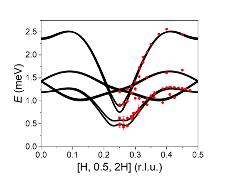
Figure 2: (Color online) Spin wave dispersion along [H,0.5,2H] direction through the magnetic peak (0.25,0.5,0.5), the experimental data (red points) are taken from Ref.Xiao2016 , with the lowest branch at $\approx$0.45 meV previously ascribed to electromagnon excitation mode $\omega_{2}$, fitted by the spin-canting model (solid line).

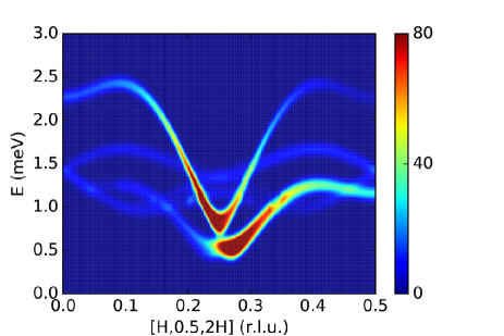
Figure 3: (Color online) Spin wave spectrum along [H,0.5,2H] direction through the magnetic peak (0.25,0.5,0.5), with Gaussian function convoluted. The color code denotes the INS intensity.

Fig. 4 is spin wave dispersion along [0.25,K,0.5]. The fitting results exhibit acceptable agreement with the measured spin wave excitations, with all parameters listed in Table I, along with previous experimental and theoretical studies. The low-lying energy excitations located in the zone centre may still be described by the spin-canting model, although one of the spin wave branches does not match the experimental data perfectly. In Fig.5, the magnetic scattering spectrum calculated in [0.25,K,0.5] crossing the magnetic reflection (0.25,0.5,0.5) also properly describes the observed scattering intensity map (Fig. 4a in Ref. Ye2011 ), where for the lowest branch the measured scattering intensity is strong on both sides of the magnetic zone centre.

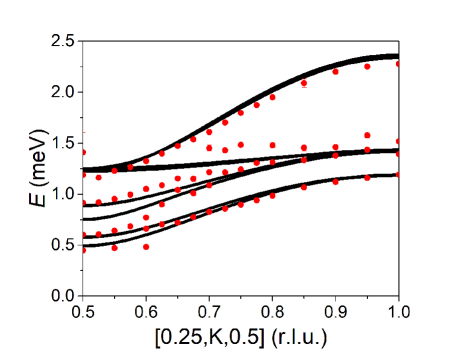
Figure 4: (Color online) Spin wave dispersion relationship along [0.25,K,0.5] direction, the experimental data (red points) are taken from Ref. Xiao2016 , fitted by the spin-canting model (solid line).

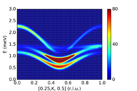
Figure 5: (Color online) Spin wave excitation spectrum along [0.25,K,0.5] direction through the magnetic peak (0.25,0.5,0.5).

Taking into account the spin wave dispersion along the high symmetry directions mentioned above, the neutron scattering intensity maps calculated with the two differently spin-canted magnetic moments at Mn_a and Mn_b are quite consistent with the observed neutron scattering spectra. Since 11 parameters are sufficient to show a good agreement with the observed data, the current study involves no further parameters dictating the magnetic coupling of Mn-Mn pairs with a longer interaction distance. However, the present model is still impossible to describe the other low-lying energy excitation mode $\omega_{1}$=0.07 meV observed in Ref.Xiao2016 . One promising technique to clarify the origin or the character of this excitation is polarized neutron scattering.

IV IV. CONCLUSIONS

In the presence of two spin-canting textures relying on a weak intrinsic polarity in the nuclear structure of MnWO₄, a more reliable model for theoretical spin-wave excitations could be provided for its AF1 phase. In comparison with previous inelastic neutron scattering spectra, it is shown that the spin-wave dispersions of this phase could be properly described by a Heisenberg model with 11 magnetic exchange couplings and single-ion anisotropy parameters. It is confirmed that long-range AF interactions are dominant in AF1 as our spin-wave dispersion relationship could be fitted well with all negative exchanging coupling constants. A strong variation in their magnitudes with increasing the Mn-Mn distance reflects strongly geometrically frustrated zigzag-like spin chains in AF1.

It should be noted that recent neutron scattering experiment observed two low energy excitations $\omega_{1}$ and $\omega_{2}$ with energy gaps at 0.07 meV and 0.45 meV, respectively Xiao2016 . Both of them cannot be described by the Heisenberg Hamiltonian based on the previous collinearly aligned spin configuration $\uparrow\uparrow\downarrow\downarrow$. In previous work, they were regarded as electromagnon excitations which might arise from the DM interaction. Interestingly, with the new non-collinear magnetic model, the $\omega_{2}$ excitation mode is properly described and we assume that it could be the lowest spin wave branch. However, our model still failed to interpret the other low-lying excitation mode $\omega_{1}$ with energy gap of 0.07 meV at the magnetic zone centre. Further polarized neutron scattering measurements would be helpful to understand the nature of this excitation as well as the mechanism of magnetoelectric coupling in MnWO₄.

References

• (1) M. Maczka, M. Ptak, A. Pikul, L. Kepiński, P. Tomaszewski, J. Hanuza, Vibrational Spectroscopy 58, 163-168 (2012).
• (2) T. Kimura, T. Goto, H. Shintani, K. Ishizaka, T. Arima, and Y. Tokura, Nature 426, 55 (2003).
• (3) T. Goto, T. Kimura, G. Lawes, A. P. Ramirez, and Y. Tokura, Phys. Rev. Lett. 92, 257201 (2004).
• (4) N. Hur, S. Park, P. A. Sharma, J.S. Ahn, S. Guha, and S.-W. Cheong, Nature 429, 392 (2004).
• (5) D. Higashiyama, S. Miyasaka, and Y. Tokura, Phys. Rev. B 72, 064421 (2005).
• (6) Y. Yamasaki, S. Miyasaka, Y. Kaneko, et al., Phys. Rev. Lett. 96, 207204 (2006).
• (7) H. Katsura, N. Nagaosa, and A. V. Balatsky, Phys. Rev. Lett. 95, 057205 (2005).
• (8) M. Mostovoy, Phys. Rev. Lett. 96, 067601 (2006).
• (9) A. B. Harris, Phys. Rev. B 76, 054447 (2007).
• (10) T. Arima, J. Phys. Soc. Jpn. 76, 073702 (2007).
• (11) I. A. Sergienko, E. Dagotto, Phys. Rev. B, 73, 094434 (2006).
• (12) L. C. Chapon, P. G. Radaelli, G. R. Blake, S. Park, and S. -W. Cheong, Phys. Rev. Lett. 96, 097601 (2006).
• (13) M. Kenzelmann, A. B. Harris, S. Jonas, et al., Phys. Rev. Lett. 95, 087206 (2005).
• (14) T. Arima, A. Tokunaga, T. Goto, H. Kimura, Y. Noda, and Y. Tokura, Phys. Rev. Lett. 96, 097202 (2006).
• (15) Y. Aharonov and A. Casher, Phys. Rev. Lett. 53, 319 (1984).
• (16) K. Taniguchi, N. Abe, T. Takenobu, Y. Iwasa, and T. Arima, Phys. Rev. Lett. 97, 097203 (2006).
• (17) A. H. Arkenbout, T. T. M. Palstra, T. Siegrist, and T. Kimura, Phys. Rev. B 74, 184431 (2006).
• (18) H. Mitamura, T. Sakakibara, H. Nakamura, T. Kimura, and K. Kindo, J. Phys. Soc. Jpn. 81, 054705 (2012).
• (19) H. Dachs, Solid State Commun. 7, 1015-1017 (1969).
• (20) G. Lautenschlaeger, H. Weitzel, T. Vogt, R. Hock, A. Boehm, M. Bonnet, H. Fuess, Phys. Rev. B 48, 6087-6098 (1993).
• (21) S.-H. Park, B. Mihailova, B. Pedersen, C. Paulmann, D. Behal, U. Gattermann, R. Hochleitner, J. Mag. Mag. Mater. 394, 160-172 (2015).
• (22) U. Gattermann, B. Roeska, C. Paulmann, S. -H. Park, J. Cryst. Growth, 453, 40-48 (2016).
• (23) U. Gattermann, S. -H. Park, C. Paulmann, G. Benka, C. Pfleiderer, J. Solid State Chemistry, 244,140-150 (2016).
• (24) S.-H. Park, B. Liu, D. Behal, B. Pedersen, A. Schneidewind, J. Phys. Condens. Matter 30, 135802 (2018).
• (25) H. Ehrenberg, H. Weitzel, H. Fuess, and B. Hennion, J. Phys. Condens. Matter 11, 2649 (1999).
• (26) H. Ehrenberg, Thesis Darmstaddt University of Technology, (1996).
• (27) F. Ye, R. S. Fishman, J. A. Fernandez-Baca, A. A. Podlesnyak, G. Ehlers, H. A. Mook, Y. Wang, B. Lorenz, and C. W. Chu, Phys. Rev. B 83, 140401(R) (2011).
• (28) Y. Xiao, C. M. N. Kumar, S. Nandi, Y. Su, W. T. Jin, Z. Fu, E. Faulhaber, A. Schneidewind, and Th. Brueckel, Phys. Rev. B 93, 214428 (2016).
• (29) C. Tian et al., Phys. Rev. B 80, 104426 (2009).
• (30) Y. A. Izyumov and R. P. Ozerov, Magnetic neutron diffraction (Plenum Press, New York,1970).
• (31) T. Holstein and H. Primakoff, Phys. Rev. 58, 1098 (1940).
• (32) R. M. White, M. Sparks, and I. Ortenburger, Phys. Rev. 139, A450 (1965).
• (33) S. W. Lovesey, Theory of Neutron Scattering from Condensed Matter (Oxford University Press, Oxford, 1984).
• (34) T. B. S. Jensen, Ph.D. thesis, Magnetic structures, phase diagram and spin waves of magneto-electric LiNiPO4.
• (35) T. B. S. Jensen, N. B. Christensen, M. Kenzelmann, H. M. R${\o}$nnow, C. Niedermayer, N. H. Andersen, K. Lefmann, M. Jimenez-Ruiz, F. Demmel, J. Li, J. L. Zarestky, and D. Vaknin, Phys. Rev. B 79, 092413 (2009).