Nonkinematic solar dynamo models with double-cell meridional circulation

Abstract

Employing the standard solar interior model as input we construct a dynamically-consistent nonlinear dynamo model that takes into account the detailed description of the $\Lambda$- effect, turbulent pumping, magnetic helicity balance, and magnetic feedback on the differential rotation and meridional circulation. The background mean-field hydrodynamic model of the solar convection zone accounts the solar-like angular velocity profile and the double-cell meridional circulation. We investigate an impact of the nonlinear magnetic field generation effects on the long-term variability and properties of the magnetic cycle. The nonlinear dynamo solutions are studied in the wide interval of the $\alpha$ effect parameter from a slightly subcritical to supercritical values. It is found that the magnetic cycle period decreases with the increasing cycle’s magnitude. The periodic long-term variations of the magnetic cycle are excited in case of the overcritical $\alpha$ effect. These variations result from the hemispheric magnetic helicity exchange. It depends on the magnetic diffusivity parameter and the magnetic helicity production rate. The large-scale magnetic activity modifies the distribution of the differential rotation and meridional circulation inside convection zone. It is found that the magnetic feedback on the global flow affects the properties of the long-term magnetic cycles. We confront our findings with solar and stellar magnetic activity observations.

1 Introduction

There is a commonly accepted idea that the sunspot activity is produced by the large-scale toroidal magnetic field which is generated inside the convection zone by means of the differential rotation [53]. The theory explains the 11-year solar cycle as a result of the large-scale dynamo operating in the solar interior, where, in addition to the magnetic fields generated by the differential rotation, the helical convective motions transforms the energy of the toroidal magnetic fields to poloidal. The effect of meridional circulation on the large-scale dynamo is not well understood. It is the essential part of the flux-transport dynamo model scenario [13, 12] to explain the equatorward drift of the toroidal magnetic field in the solar cycle. Here, it assumed that the toroidal field at the bottom of the convection zone forms sunspot activity. Feasibility of this idea can be questioned both the observational and theoretical arguments [6]. The distributed dynamo models can be constructed with [4, 26, 56] and without [50, 71] effect of meridional transport of the large-scale magnetic field.

Recent results of helioseismology reveal the double-cell meridional circulation structure [93, 5]. It demolishes the previously accepted scenario of the flux-transport models [22, 86, 23]. Contrary, Pipin and Kosovichev [66] showed the distributed dynamo models can reproduce observations with regards to the subsurface rotational shear layer and the double-cell meridional circulation. In their model, the double-cell meridional circulation was modeled in following to results of helioseismology of Zhao et al. [93]. The effect of the multi-cell meridional circulation on the global dynamo was also studied in the direct numerical simulations [30, 19, 85]. There were no attempts to construct the non-kinematic mean-field dynamo models with regards to the multi-cell meridional circulation.

The standard mean-field models of the solar differential rotation predict a one-cell meridional circulation per hemisphere. This contradicts to the helioseismology inversions and results of direct numerical simulations. In the mean-field theory framework, the differential rotation of the Sun is explained as a result of the angular momentum transport by the helical convective motions. Similarly to a contribution of the $\alpha$ effect in the mean-electromotive force, i.e.,

$$\mathbf{\mathcal{E}}=\left\langle\mathbf{u}\times\mathbf{b}\right\rangle=\hat{\alpha}\circ\left\langle\mathbf{B}\right\rangle+\dots,$$

where $\mathbf{u}$ is the turbulent velocity $\mathbf{u}$, and $\mathbf{b}$ is the turbulent magnetic field, the $\Lambda$-effect, (e.g., 77) appears as the non-dissipative part of turbulent stresses

$$\hat{T}_{ij}=\left\langle u_{i}u_{j}\right\rangle=\Lambda_{ijk}\Omega_{k}+\dots$$

where $\boldsymbol{\Omega}$ is the angular velocity. The structure of the meridional circulation is determined by directions of the non-diffusive angular momentum transport due to the $\Lambda$ effect [1]. In particular, the vertical structure of the meridional circulation depends on the sign of the radial effect. It was found that the double-cell meridional circulation can be explained if the of $\Lambda$-effect changes sign in the depth of the convection zone. Pipin and Kosovichev [68] showed that this effect can result from the radial inhomogeneity of the convective turnover timescale. It was demonstrated that if this effect is taken into account then the solar-like differential rotation and the double-cell meridional circulation are both reproduced by the mean-field model .

In this paper, we apply the meridional circulation profile, which is calculated from the solution of the angular momentum balance to the nonkinematic dynamo models. Previously, the similar approach was applied by Brandenburg et al. [8] and Rempel [74] in the distributed and the flux-transport models with one meridional circulation cell as the basic stage in the non-magnetic case.

Our main goal is to study how the double-cell meridional circulation affects the nonlinear dynamo generation of the large-scale magnetic field. The magnetic feedback on the global flow can result in numerous physical phenomena such as the torsional oscillations [45, 24], the long-term variability of the magnetic activity [79, 16] etc. The properties of the nonlinear evolution depend on the dynamo governing parameters such as amplitude of turbulent generation of the magnetic field by the $\alpha$ effect, as well as the other nonlinear processes involved in the dynamo, i.e., the dynamo quenching by the magnetic buoyancy effect [35, 83] and the magnetic helicity conservation [39]. We study if the long-term variation of magnetic activity can result from the increasing level of turbulent generation of magnetic field by the $\alpha$ effect. The increasing of the $\alpha$ effect results to an increase of the magnetic helicity production. This affects the large-scale magnetic field generation by means of the magnetic helicity conservation. Hence, the magnetic helicity balance has to be taken into account.

It is hardly possible to consider in full all the goals within one paper. From our point of view, the most important tasks includes: construction of the solar-type dynamo model with the multi-cell meridional circulation and studying the principal nonlinear dynamo effects. The latter includes the magnetic helicity conservation and the nonkinematic effects due to the magnetic feedback on the large-scale flow. Accordingly, the paper is organized as follows. Next Section describes the hydrodynamic, thermodynamic and magnetohydrodynamic parts of the model. Then, I present an attempt to construct the solar-type dynamo model and discuss the effect of the turbulent pumping on the properties of the dynamo solution. The next subsections consider result for the principal nonlinear dynamo effects. They deals with the global flows variations, the Grand activity cycles and the magnetic cycle variations of the thermodynamic parameters in the model. The paper is concluded with a discussion of the main results using results of other theoretical studies and results of observations.

2 Basic equations.

2.1 The angular momentum balance

We consider the evolution of the axisymmetric large-scale flow, which is decomposed into poloidal and toroidal components: $\mathbf{\overline{U}}=\mathbf{\overline{U}}^{m}+r\sin\theta\Omega\hat{\mathbf{\boldsymbol{\phi}}}$, where $\boldsymbol{\hat{\phi}}$ is the unit vector in the azimuthal direction. The mean flow satisfies the stationary continuity equation,

$$\boldsymbol{\nabla}\cdot\overline{\rho}\mathbf{\overline{U}}=0,$$ (1)

Distribution of the angular velocity inside convection zone is determined by conservation of the angular momentum [77]:

$$\frac{\partial}{\partial t}\overline{\rho}r^{2}\sin^{2}\theta\Omega = -\boldsymbol{\nabla\cdot}\left(r\sin\theta\overline{\rho}\left(\hat{\mathbf{T}}_{\phi}+r\sin\theta\Omega\mathbf{\overline{U}^{m}}\right)\right)$$

$$+ \boldsymbol{\nabla\cdot}\left(r\sin\theta\frac{\overline{\mathbf{B}}\overline{B}_{\phi}}{4\pi}\right).$$

To determine the meridional circulation we consider the azimuthal component of the large-scale vorticity , $\omega=\left(\boldsymbol{\nabla}\times\overline{\mathbf{U}}^{m}\right)_{\phi}$ , which is governed by equation:

$$\frac{\partial\omega}{\partial t}\!\!\! \negthinspace\!=\!\!\!\! r\sin\theta\boldsymbol{\nabla}\cdot\left(\frac{\hat{\boldsymbol{\phi}}\times\boldsymbol{\nabla\cdot}\overline{\rho}\hat{\mathbf{T}}}{r\overline{\rho}\sin\theta}-\frac{\mathbf{\overline{U}}^{m}\omega}{r\sin\theta}\right)\!\!+r\sin\theta\frac{\partial\Omega^{2}}{\partial z}$$

$$+\!\!\! \frac{1}{\overline{\rho}^{2}}\left[\boldsymbol{\nabla}\overline{\rho}\times\boldsymbol{\nabla}\overline{p}\right]_{\phi}\!\!$$

$$+ \!\frac{1}{\overline{\rho}^{2}}\left[\!\!\boldsymbol{\nabla}\overline{\rho}\times\left(\!\!\boldsymbol{\nabla}\frac{\overline{\mathbf{B}}^{2}}{8\pi}-\frac{\left(\overline{\mathbf{B}}\boldsymbol{\cdot\nabla}\right)\overline{\mathbf{B}}}{4\pi}\!\right)\!\!\right]_{\phi},$$

The turbulent stresses tensor, $\hat{\mathbf{T}}$, is written in terms of small-scale fluctuations of velocity and magnetic field:

$$\hat{T}_{ij}=\left(\left\langle u_{i}u_{j}\right\rangle-\frac{1}{4\pi\overline{\rho}}\left(\left\langle b_{i}b_{j}\right\rangle-\frac{1}{2}\delta_{ij}\left\langle\mathbf{b}^{2}\right\rangle\right)\right).$$ (4)

where ${\partial/\partial z=\cos\theta\partial/\partial r-\sin\theta/r\cdot\partial/\partial\theta}$ is the gradient along the axis of rotation. The turbulent stresses affect generation and dissipation of large-scale flows, and they are affected by the global rotation and magnetic field. The magnitude of the kinetic coefficients in tensor $\hat{\mathbf{T}}$ depends on the rms of the convective velocity, ${u}^{\prime}$, the strength of the Coriolis force and the strength of the large-scale magnetic field. The effect of the Coriolis force is determined by parameter $\Omega^{*}=2\Omega_{0}\tau_{c}$, where $\Omega_{0}=2.9\times 10^{-6}$rad/s is the solar rotation rate and $\tau_{c}$ is the convective turnover time. The effect of the large-scale magnetic field on the convective turbulence is determined by parameter $\beta=\left\langle\left|\mathbf{B}\right|\right\rangle/\sqrt{4\pi\overline{\rho}u^{\prime 2}}$.

The magnetic feedback on the coefficients of turbulent stress tensor $\hat{\mathbf{T}}$ was studied previously with the mean-field magnetohydrodynamic framework [75]. In our model we apply analytical results of Kitchatinov et al. [36], Kitchatinov et al. [38] and Kueker et al. [43]. The analytical expression for $\hat{\mathbf{T}}$ is given in Appendix. It was found that the standard components of the nondissipative of $\hat{\mathbf{T}}$ ($\Lambda$-effect) are quenched with the increase of the magnetic field strength as $\beta^{-2}$ and the magnetic quenching of the viscous parts is the order of $\beta^{-1}$. Also, there is a non-trivial effect inducing the latitudinal angular momentum flux proportional to the magnetic energy [38, 43]. This effect is quenched as $\beta^{-2}$ for the case of the strong magnetic field. Implications of the magnetic feedback on the turbulent stress tensor $\hat{\mathbf{T}}$ were discussed in the models of solar torsional oscillations and Grand activity cycles [38, 43, 59, 44]. The analytical results of the mean-field theory are in qualitative agreement with the direct numerical simulations [28, 31, 27].

Profile of $\tau_{c}$ (as well as profiles of $\overline{\rho}$ and other thermodynamic parameters) is obtained from a standard solar interior model calculated using the MESA code [57, 58]. The rms velocity, $u^{\prime}$, is determined in the mixing length approximations from the gradient of the mean entropy, $\overline{s}$,

$$u^{\prime}=\frac{\ell}{2}\sqrt{-\frac{g}{2c_{p}}\frac{\partial\overline{s}}{\partial r}},$$ (5)

where $\ell=\alpha_{MLT}H_{p}$ is the mixing length, $\alpha_{MLT}=2.2$ is the mixing length theory parameter, and $H_{p}$ is the pressure scale height. For a non-rotating star the ${u}^{\prime}$ profile corresponds to results of the MESA code. The mean-field equation for heat transport takes into account effects of rotation and magnetic field [63]:

$$\overline{\rho}\overline{T}\left(\frac{\partial\overline{s}}{\partial t}+\left(\overline{\mathbf{U}}\cdot\boldsymbol{\nabla}\right)\overline{s}\right)=-\boldsymbol{\nabla}\cdot\left(\mathbf{F}^{conv}+\mathbf{F}^{rad}\right)-\hat{T}_{ij}\frac{\partial\overline{U}_{i}}{\partial r_{j}}-\frac{1}{4\pi}\boldsymbol{\mathcal{E}}\cdot\nabla\times\boldsymbol{\overline{B}},$$ (6)

where, $\overline{\rho}$ and $\overline{T}$ are the mean density and temperature, $\boldsymbol{\mathcal{E}}=\left\langle\mathbf{u\times b}\right\rangle$ is the mean electromotive force. The Eq.(6) includes the thermal energy loss and gain due to generation and dissipation of large-scale flows. The last term of the Eq.(6) takes into account effect of thermal energy exchange because of dissipation and generation of magnetic field [63]. In derivation of the mean-field heat transport equation (see, 63), it was assumed that the magnetic and rotational perturbations of the reference thermodynamic state are small. Also the parameters of the reference state are given independently by the MESA code.

For the anisotropic convective flux we employ the expression suggested by Kitchatinov et al. [36] (hereafter KPR94),

$$F_{i}^{conv}=-\overline{\rho}\overline{T}\chi_{ij}\nabla_{j}\overline{s}.$$ (7)

The further details about dependence of the eddy conductivity tensor $\chi_{ij}$ from effects of both the global rotation and large-scale magnetic field are given in Appendix. The diffusive heat transport by radiation reads,

$$\mathbf{F}^{rad}=-c_{p}\overline{\rho}\chi_{D}\boldsymbol{\nabla}T,$$

where

$$\chi_{D}=\frac{16\sigma\overline{T}^{3}}{3\kappa\overline{\rho}^{2}c_{p}}.$$

Both the eddy conductivity and viscosity are determined from the mixing-length approximation:

$$\chi_{T} = \frac{\ell^{2}}{4}\sqrt{-\frac{g}{2c_{p}}\frac{\partial\overline{s}}{\partial r}},$$ (8)

$$\nu_{T} = \mathrm{Pr_{T}}\chi_{T},$$ (9)

where $\mathrm{Pr_{T}}$ is the turbulent Prandtl number. Note, that in Eq(8) we employ factor $1/2$ instead of $1/3$. With this choice the distribution of the mean entropy gradient, which results from solution of the Eq(6) for the nonrotating and nonmagnetic case is close to results of the MESA code. It is assumed that $\mathrm{Pr_{T}}={\displaystyle 3/4}$. This corresponds to the theoretical results of KPR94. For this choice we have the good agreement with solar angular velocity latitudinal profile. We assume that the solar rotation rate corresponds to rotation rate of solar tachocline at 30^∘ latitude, i.e., $\Omega_{0}/2\pi=430$nHz [41]. We employ the stress-free boundary conditions in the hydrodynamic part of the problem. For the Eq(6) the thermal flux at the bottom is taken from the MESA code. At the top, the thermal flux from the surface is approximated by the flux from a blackbody:

$$F_{r}=\frac{L_{\odot}}{4\pi r^{2}}\left(1+4\frac{T_{e}}{T_{eff}}\frac{\overline{s}}{c_{p}}\right),$$ (10)

where where $T_{eff}$ is the effective temperature of the photosphere and $T_{e}$ is the temperature at the outer boundary of the integration domain.

Figure 1 shows profiles of the angular velocity, streamlines of the meridional circulations and the radial profiles of the angular velocity and the meridional flow velocity for a set of latitudes. The given results were discussed in details by Pipin and Kosovichev [68]. The model shows the double-layer circulation pattern with the upper stagnation point at $r=0.88R_{\odot}$. The amplitude of the surface poleward flow is about 15m/s. The angular velocity profile shows a strong subsurface shear that is higher at low latitudes and it is less near poles. Contrary to results of Zhao et al. [93] and model of Pipin and Kosovichev [66] the double-cell meridional circulation structure extends from equator to pole. This is partly confirmed by the new results of helioseismology by Chen and Zhao [11] who also found that the poleward flow at the surface goes close enough to pole. It is important no mention that the current results of the helioseismic inversions for the meridional circulation remains controversial For example, Rajaguru and Antia [72] found that the meridional circulation can be approximated by a single-cell structure with the return flow deeper than 0.77R_⊙. However, their results indicate an additional weak cell in the equatorial region, and contradict to the recent results of Böning et al. [5] who confirmed a shallow return flow at 0.9R_⊙. Also, their results indicated that the upper meridional circulation cell extends close to the solar pole.

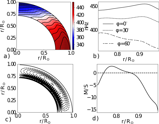
Figure 1: a) angular velocity profile, $\Omega\left(r,\theta\right)/2\pi$, contours are in range of 327-454 nHz; b) the radial profiles of the angular velocity for latitudes: $\varphi=0^{\circ}$, $30^{\circ}$ and $60^{\circ}$; c) streamlines of the meridional circulation; d) radial profile of the meridional flow at $\theta=45^{\circ}$.

2.2 Dynamo equations

We model evolution of the large-scale axisymmetric magnetic field, $\overline{\mathbf{B}}$, by the mean-field induction equation [42],

$$\partial_{t}\overline{\mathbf{B}}=\boldsymbol{\nabla}\times\left(\boldsymbol{\mathcal{E}}+\mathbf{\overline{U}}\times\overline{\mathbf{B}}\right),$$ (11)

where, $\boldsymbol{\mathcal{E}}=\left\langle\mathbf{u\times b}\right\rangle$ is the mean electromotive force with $\mathbf{u}$ and $\mathbf{b}$ standing for the turbulent fluctuating velocity and magnetic field respectively.

Similar to our recent paper (see, [67, 62]), we employ the mean electromotive force in form:

$$\mathcal{E}_{i}=\left(\alpha_{ij}+\gamma_{ij}\right)\overline{B}_{j}-\eta_{ijk}\nabla_{j}\overline{B}_{k}.$$ (12)

where symmetric tensor $\alpha_{ij}$ models the generation of magnetic field by the $\alpha$- effect; antisymmetric tensor$\gamma_{ij}$ controls the mean drift of the large-scale magnetic fields in turbulent medium, including the magnetic buoyancy; the tensor $\eta_{ijk}$ governs the turbulent diffusion. The reader can find further details about the $\boldsymbol{\mathcal{E}}$ in the above cited papers.

The $\alpha$ effect takes into account the kinetic and magnetic helicities in the following form:

$$\alpha_{ij} = C_{\alpha}\eta_{T}\psi_{\alpha}(\beta)\alpha_{ij}^{(H)}+\alpha_{ij}^{(M)}\frac{\overline{\chi}\tau_{c}}{4\pi\overline{\rho}\ell^{2}},$$ (13)

$$\eta_{T} = \frac{\nu_{T}}{\mathrm{Pm_{T}}}$$ (14)

where $C_{\alpha}$ is a free parameter which controls the strength of the $\alpha$- effect due to turbulent kinetic helicity; tensors $\alpha_{ij}^{(H)}$ and $\alpha_{ij}^{(M)}$ express the kinetic and magnetic helicity parts of the $\alpha$-effect, respectively; $\mathrm{Pm_{T}}$ is the turbulent magnetic Prandtl number, and $\overline{\chi}=\left\langle\mathbf{a}\cdot\mathbf{b}\right\rangle$ ($\mathbf{a}$ and $\mathbf{b}$ are the fluctuating parts of magnetic field vector-potential and magnetic field vector). Both the $\alpha_{ij}^{(H)}$ and the $\alpha_{ij}^{(M)}$ depend on the Coriolis number. Function $\psi_{\alpha}(\beta)$ controls the so-called “algebraic” quenching of the $\alpha$- effect where $\beta=\left|\overline{\mathbf{B}}\right|/\sqrt{4\pi\overline{\rho}u^{\prime 2}}$, $u^{\prime}$ is the RMS of the convective velocity. It is found that $\psi_{\alpha}(\beta)\sim\beta^{-3}$ for $\beta\gg 1$. The $\alpha$- effect tensors $\alpha_{ij}^{(H)}$ and $\alpha_{ij}^{(M)}$ are given in Appendix.

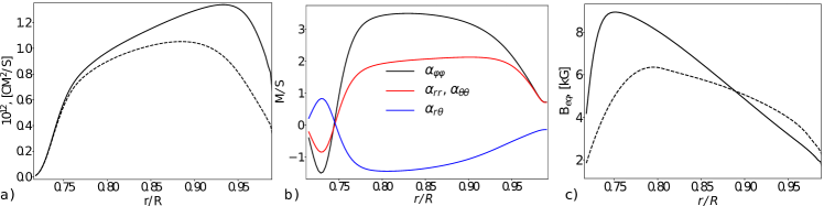
Figure 2: a) the radial profiles of the total (solid line) and anisotropic (dashed line) parts of the eddy diffusivity at $\theta=45^{\circ}$; b) radial profiles of the kinetic $\alpha$-effect components at $\theta=45^{\circ}$; c) the equipartition strength of the magnetic field, $B_{eq}=\sqrt{4\pi\overline{\rho}u^{\prime 2}}$, where $u^{\prime}$ is determined by the equatorial profile of the mean entropy, see the Eq(5); the dashed line is from results of the reference model (MESA code) and the solid line is for the rotating convection zone,i.e., after solution of the Eq(6).

Contribution of the magnetic helicity to the $\alpha$-effect is expressed by the second term in Eq.(13). The evolution of the turbulent magnetic helicity density, $\overline{\chi}=\left\langle\mathbf{a}\cdot\mathbf{b}\right\rangle$, is governed by the conservation law [71]:

$$\frac{\partial\overline{\chi}}{\partial t} = -2\left(\boldsymbol{\mathcal{E}}\cdot\overline{\bm{B}}\right)-\frac{\overline{\chi}}{R_{m}\tau_{c}}+\boldsymbol{\nabla}\cdot\left(\eta_{\chi}\boldsymbol{\nabla}\bar{\chi}\right)$$

$$-\eta\overline{\mathbf{B}}\cdot\mathbf{\overline{J}}-\boldsymbol{\nabla}\cdot\left(\boldsymbol{\mathcal{E}}\times\overline{\mathbf{A}}\right),$$

where $R_{m}=10^{6}$ is the magnetic Reynolds number and $\eta$ is the microscopic magnetic diffusion. In the drastic difference to anzatz of Kleeorin and Ruzmaikin [39], the Eq(2.2) contains the term $\left(\boldsymbol{\mathcal{E}}\times\overline{\mathbf{A}}\right)$. It consists of the magnetic helicity density fluxes which result from the large-scale magnetic dynamo wave evolution. The given contribution alleviates the catastrophic quenching problem [25, 71]. Also the catastrophic quenching of the $\alpha$-effect can be alleviated with help of the diffusive flux of the turbulent magnetic helicity, $\boldsymbol{\boldsymbol{\mathcal{F}}}^{\chi}=-\eta_{\chi}\boldsymbol{\nabla}\bar{\chi}$ [18, 10]. The coefficient of the turbulent helicity diffusivity, $\eta_{\chi}$, is a parameter in our study. It affects the hemispheric helicity transfer [48].

In the model we take into account the mean drift of large-scale field due to the magnetic buoyancy, $\gamma_{ij}^{(buo)}$ and the gradient of the mean density, $\gamma_{ij}^{(\Lambda\rho)}$:

$$\gamma_{ij} = \gamma_{ij}^{(\Lambda\rho)}+\gamma_{ij}^{(buo)},$$

$$\gamma_{ij}^{(\Lambda\rho)} = 3C_{pum}\eta_{T}\left(f_{1}^{(a)}\left(\mathbf{\boldsymbol{\Omega}}\cdot\boldsymbol{\Lambda}^{(\rho)}\right)\frac{\Omega_{n}}{\Omega^{2}}\varepsilon_{inj}-\frac{\Omega_{j}}{\Omega^{2}}\varepsilon_{inm}\Omega_{n}\Lambda_{m}^{(\rho)}\right)$$ (16)

$$\gamma_{ij}^{(buo)} = -\frac{\alpha_{MLT}u^{\prime}}{\gamma}\beta^{2}K\left(\beta\right)g_{n}\varepsilon_{inj},$$

where $\mathbf{\boldsymbol{\Lambda}}^{(\rho)}=\boldsymbol{\nabla}\log\overline{\rho}$ ; functions $f_{1}^{(a)}$ and $K\left(\beta\right)$ are given in [35, 62]. The standard choice of the pumping parameter is $C_{pum}=1$. In this case the pumping velocity is scaled in the same way as the magnetic eddy diffusivity. In the presence of the multi-cell meridional circulation, the direction and magnitude of the turbulent pumping become critically important for the modelled evolution of the magnetic field. It is confirmed in the direct numerical simulations, as well (see, [85]). For the standard choice, the turbulent pumping is about an order of magnitude less than the meridional circulation. For this case, explanation of the latitudinal drift of the toroidal magnetic field near the surface faces a problem (cf., [66]). To study the effect of turbulent pumping we introduce this parameter $C_{pum}$.

For the bottom boundary we apply the perfect conductor boundary conditions: $\mathcal{E}_{\theta}=0,\,A=0$. The boundary conditions at the top are defined as follows. Firstly, following ideas of Moss and Brandenburg [49] and Pipin and Kosovichev [65] we formulate the boundary condition in the form that allows penetration of the toroidal magnetic field to the surface:

$$\delta\frac{\eta_{T}}{r_{e}}B+\left(1-\delta\right)\mathcal{E}_{\theta} = 0,$$ (17)

where $r_{e}=0.99R_{\odot}$, and parameter $\delta=0.99$. The magnetic field potential in the outside domain is

$$A^{(vac)}\left(r,\mu\right)=\sum a_{n}\left(\frac{r_{e}}{r}\right)^{n}\sqrt{1-\mu^{2}}P_{n}^{1}\left(\mu\right).$$ (18)

The coupled angular momentum and dynamo equations are solved using finite differences for integration along the radius and the pseudospectral nodes for integration in latitude. The number of mesh points in radial direction was varied from $100$ to $150$. The nodes in latitude are zeros of the Legendre polynomial of degree ${N}$, where N was varied from ${N=64}$ to ${N=84}$. The resolution with 64 nodes in latitude and with 100 points in radius was found satisfactory. The model employed the Crank-Nicolson scheme, using a half of the time-step for integration in the radial direction and another half for integration along latitude.

To quantify the mirror symmetry type of the toroidal magnetic field distribution relative to equator we introduce the parity index $P$:

$$P = \frac{E_{q}-E_{d}}{E_{q}+E_{d}},$$ (19)

$$E_{d} = \int\left(B\left(r_{0},\theta\right)-B\left(r_{0},\pi-\theta\right)\right)^{2}\sin\theta d\theta,$$

$$E_{q} = \int\left(B\left(r_{0},\theta\right)+B\left(r_{0},\pi-\theta\right)\right)^{2}\sin\theta d\theta,$$

where $E_{d}$ and $E_{q}$ are the energies of the dipole-like and quadruple-like modes of the toroidal magnetic field at $r_{0}=0.9R_{\odot}$. Another integral parameter is the mean density of the toroidal magnetic field in the subsurface shear layer:

$$\overline{B^{T}}=\sqrt{E_{d}+E_{q}}.$$ (20)

Another parameter characterize the mean strength of the dynamo processes in the convection zone:

$$\overline{\beta}=\left\langle\left|\overline{\mathbf{B}}\right|/\sqrt{4\pi\overline{\rho}u^{\prime 2}}\right\rangle,$$ (21)

where the averaging is done over the convection zone volume. The boundary conditions Eq(17) provide the Poynting flux of the magnetic energy out of the convection zone. Taking into account the Eq(10) the variation of the thermal flux at the surface are given as follows:

$$\delta F = \delta F_{c}+\delta F_{B}$$ (22)

$$\delta F_{c} = 4\frac{T_{e}}{T_{eff}}\frac{\delta\overline{s}}{c_{p}}$$ (23)

$$\delta F_{B} = \frac{1}{4\pi}\left(\mathcal{E}_{\phi}\overline{B}_{r}-\mathcal{E}_{\theta}\overline{B}_{\phi}\right),$$ (24)

where $\delta\overline{s}$ is the entropy variation because of the magnetic activity. The second term of the Eq(22) governs the magnetic energy input in the stellar corona.

3 Results

To match the solar cycle period we put $\mathrm{Pm_{T}}=10$ in all our models. The theoretical estimations of Kitchatinov et al. [36] gives $\mathrm{Pm_{T}}=4/3$. This is the long standing theoretical problem of the solar dynamo period [9]. Currently, the solar dynamo period can be reproduced for $\mathrm{Pm_{T}}\gg 1$. The issue exists both in the distributed and in the flux-transport dynamo. Moreover, the flux-transport dynamo can reproduce the observation only with the special radial profile of the eddy diffusivity (see, e.g., [74]). In our models we employ the rotational quenching the eddy diffusivity coefficients and the high $\mathrm{Pm_{T}}$. Figures 2a and b show the radial profiles of the eddy diffusivity coefficients and components of the $\alpha_{ij}^{(H)}$ at latitude $45^{\circ}$ in our model for $\mathrm{Pm_{T}}=10$. In the upper part of the convection zone the magnitude of the turbulent magnetic diffusivity is close to estimations of Martinez Pillet et al. [47] based on observations of the sunspot decay rate. The eddy diffusivity is an order of $10^{10}$cm/s and less near the bottom of the convection zone. The diffusivity profile is the same as in our previous paper Pipin and Kosovichev [67].

The radial profiles of the $\alpha$ effect for $C_{\alpha}=C_{\alpha}^{(cr)}$ are illustrated in Figure 2b. The $\alpha$ effect (cf, the above discussion about $\Lambda$-effect) change the sign near the bottom of the convection zone. This is also found in the direct numerical simulations [29].

Table 1 gives the list of our models, their control and output parameters. We sort the models with respect to magnitude of the $\alpha$ effect using the ratio ${\displaystyle\frac{C_{\alpha}}{C_{\alpha}^{(cr)}}}$, the magnitude of the eddy-diffusivity of the magnetic helicity density, ${\displaystyle\frac{\eta_{\chi}}{\eta_{T}}}$, where $\eta_{T}=\nu_{T}/\mathrm{Pm_{T}}$, and $\nu_{T}$ is determined from Eq(9), and with respect of the magnetic feedback on the differential rotation. The $C_{pum}$ controls the pumping velocity magnitude (see, Eq(16)); the parameter ${\displaystyle\frac{\Delta\Omega}{\Omega_{0}}}$ show the relative difference of the surface angular velocity between the solar equator and pole; the strength of the dynamo is characterized by the range of the magnetic cycle variations of $\overline{\beta}$ (see, Eq(21)); the dynamo cycle period; the magnitude of the surface meridional circulation. From the Table 1 we see that the nonkinematic runs show the magnetic cycle variations of ${\displaystyle\frac{\Delta\Omega}{\Omega_{0}}}$ and the surface meridional circulation.

Figure 2b shows the radial profiles of the equipartition strength of the magnetic field, $B_{eq}=\sqrt{4\pi\overline{\rho}u^{\prime 2}}$ in the solar convection zone for the reference model (non-rotating) given by MESA code and in the rotating convective zone. In the rotating convection zone, the mean-entropy gradient is larger than in the nonrotating case. This is because of the rotational quenching of the eddy-conductivity. The magnitude of the convective heat flux is determined by the boundary condition at the bottom of the convection zone and it remains the same for the rotating (our model) and nonrotating (MESA code) cases. Assuming that the convective turnover time is not subjected to the rotational quenching, the reduction of the eddy conductivity because of the rotational quenching is compensated by the increase of the mean-entropy gradient. This results in the increase of the parameter $B_{eq}$.

The increase of the RMS convective velocity in case of the rotating convection zone seems to contradict the results of direct numerical simulations of [84]. This is likely because of inconsistent assumptions behind the MLT expression for the RMS convective velocity, see Eq(5). The given issue can affect the amplitude of the dynamo generated magnetic field near the bottom of the convection zone. Our models operate in regimes where $\left|B\right|\leq B_{eq}$, and the substantial part of the dynamo quenching is due to magnetic helicity conservation. Therefore the given issue does not much affect our results.

Table 1: Control and output parameters of the dynamo models.

Model	$C_{pum}$	${\displaystyle\frac{\eta_{\chi}}{\eta_{T}}}$	${\displaystyle\frac{C_{\alpha}}{C_{\alpha}^{(cr)}}}$	${\displaystyle\frac{\Delta\Omega}{\Omega_{0}}}$	$\overline{\beta}$	Period [YR]	$\max U_{\theta}$ [M/S]
M1	1	$0.1$	1.1	0.279	0.05-0.1	6	15
M2	PmT	0.1	1.1	0.279	0.13-0.24	10.5	15
M4	-/-	0.3	-/-	0.279	0.15-0.3	10.5,12.05	15
M5	-/-	0.01	-/-	0.279	0.14-0.26	9.3	15
			Nonkinematic	runs
M3	PmT	0.1	1.1	0.263-0.275	0.11-0.21	10.3	15.0 $\pm 0.5$
M3a2	-/-	-/-	2	0.232-0.253	0.36-0.66	4.7,265	14.0 $\pm 2.1$
M3a3	-/-	-/-	3	0.22-0.24	0.52-0.91	4.0	14.5 $\pm 2.5$
M3a4	-/-	-/-	4	0.21-0.245	0.68-1.05	3.4	14.7 $\pm 3.$5

3.1 Effects of turbulent pumping

As the first step, we consider the kinematic dynamo model with the nonlinear $\alpha$ effect. Results of the model M1 are shown in Figure 3. The model M1 roughly agree with results of Pipin and Kosovichev [66] (hereafter, PK13). It employs the same mean electromotive force as in our previous paper. In particular, the maximum pumping velocity is the order of 1m/s. The effective velocity drift due to the magnetic pumping and meridional circulation is shown in Figures 3(a) and (b). Figures 3(d) and (e) show the time-latitude variations of the toroidal magnetic field at $r=0.9R$ and in the middle of the convection zone. The agreement with the solar observations is worse than in the previous model PK13 because of difference in the meridional circulation structure. The model of PK13 employed the meridional circulation profile provided by results of Zhao et al. [93]. In that profile, the near-surface meridional circulation cell is more shallow and it does not touch the pole as it happens in the present model, see, Figure 1. By this reason, the polar magnetic field in model M1 is much larger than in results of PK13.

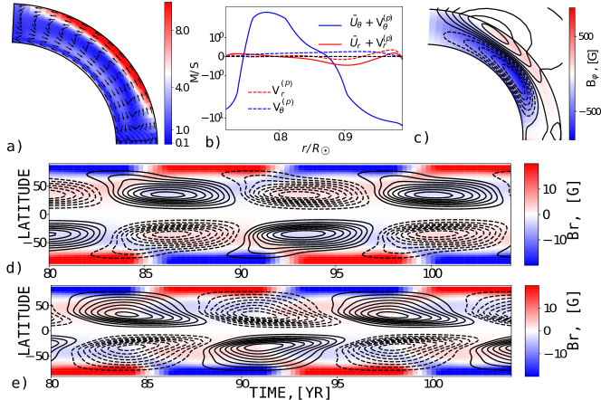
Figure 3: a) Direction of pumping velocity of the toroidal magnetic field in model M1; b) the effective velocity drift of the toroidal magnetic field (pumping + meridional circulation); c) the snapshot of the toroidal magnetic field distribution (color image) and streamlines of the poloidal magnetic field in the Northern hemisphere of the Sun; d) the time-latitude diagram of the toroidal magnetic field evolution (contours in range of of $\pm 500$G at $r=0.9R$ and radial magnetic field at the surface (color image).

For the purpose of our study, it is important to get the properties of the dynamo solution as close as possible to results of solar observations. To solve the above issues we increase the turbulent pumping velocity magnitude by factor $\mathrm{Pm_{T}}$. The results are shown in Figure 4. The model has the correct time-latitude diagram of the toroidal magnetic field in the subsurface shear layer. The surface radial magnetic field evolves in agreement with results of observations [81]. The magnitude of the polar magnetic field is 10 G, which is in a better agreement with observations (e.g., [46]) than the model M1. Figures 4 (a) and (b) show the effective velocity drift of the large-scale toroidal magnetic field. The equatorward drift with magnitude the order of 1-2 m/s operates in major part of the solar convection zone from $0.75R$ to $0.91R$. Interesting that the obtained results are similar to those from the direct numerical simulation of Warnecke et al. [85]. Note that in the given model the magnitude of the pumping velocity is about factor 2 less than in results of Warnecke et al. [85]. It seems that some of the issues in model M1 would be less pronounced if the meridional circulation pattern was closer to results of helioseismology of Zhao et al. [93] or Chen and Zhao [11]. However results of the direct numerical simulations of [84, 85] seem to show that the evolution of the large-scale magnetic field inside convection zone does not depend much on the meridional circulation. This argues for the strong magnetic pumping effects in the global dynamo. This important issue can be debated further. This is out of the main scopes of this paper. The rest of our models employ the same pumping effect as in the model M2 (see, Table 1).

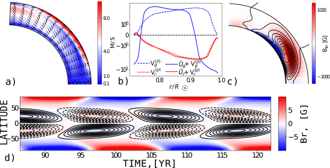
Figure 4: a) Direction of pumping velocity of the toroidal magnetic field in model M2; b) the effective velocity drift of the toroidal magnetic field (pumping + meridional circulation); c) the snapshot of the toroidal magnetic field distribution (color image) and streamlines of the poloidal magnetic field in the Northern hemisphere of the Sun; d) the time-latitude diagram of the toroidal magnetic field evolution (contours in range of of $\pm 1$kG at $r=0.9R$ and radial magnetic field at the surface (color image).

3.2 The global flows oscillations in magnetic cycle

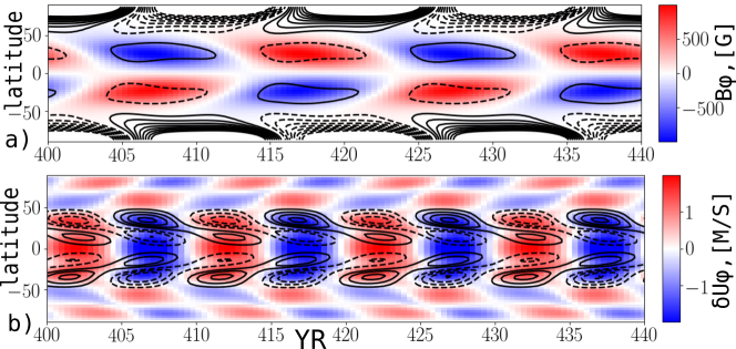
Figure 5: The model M3, a) Time-latitude butterfly diagram for the toroidal field in the upper part of the convection zone (color image) and the surface radial magnetic field shown by contours ($\pm$5G); b) the surface variations of the azimuthal velocity (color image) and the meridional velocity (contours in the range of $\pm 0.5$ m/s).

Figure 5 show the time-latitude diagrams of the magnetic field and the global flow variations for the model M3. The torsional oscillations on the surface are about $\pm 2$m/s. They are defined as follows, $\delta U_{\phi}=\left(\Omega\left(r,\theta t\right)-\overline{\Omega\left(r,\theta,t\right)}\right)r\sin\theta$, where the averaging is done over the stationary phase of evolution. The torsional wave has both the equator- and poleward branches. In the equatorward torsional wave, the change from the positive to negative variation goes about 2 years ahead of the maxima of the toroidal magnetic field wave. This agrees with results of observations of Howe et al. [24] and with direct numerical simulations of Guerrero et al. [20]. The magnitude of the meridional flow variations agrees with results of Zhao et al. [94]. Also, we see that on the surface the meridional velocity variations converge toward the maximum of the toroidal magnetic field wave. This is also in qualitative agreement with the observations.

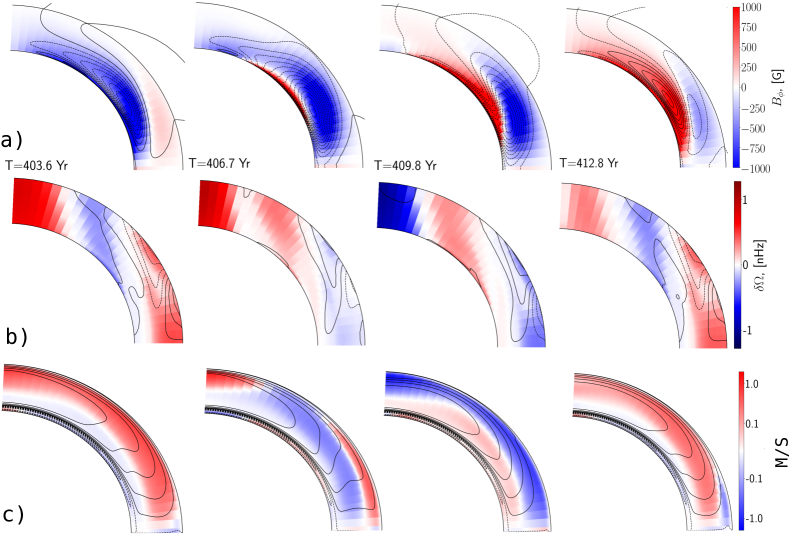
Figure 6: The model M3: a) snapshots of the magnetic field in four phase of the magnetic cycle, the toroidal magnetic field strength is shown by color, contours show streamlines of the poloidal magnetic field; b) color image show variations of the angular velocity, contours (range of $\pm 0.5$m/s) show variations of the meridional flow; c) contours show the azimuthal component of the total (kinetic and magnetic helicity parts)$\alpha$ -effect, the background image shows the part of the $\alpha_{\phi\phi}$ induced by the magnetic helicity conservation (see, the second term of Eq(13)).

Figure 6 shows snapshots of the magnetic field, the global flows variations and the azimuthal component of the total (kinetic and magnetic helicity parts)$\alpha$ -effect for a half magnetic cycle. The Figure shows that a new cycle starts at the bottom of the convection zone. The main part of the dynamo wave drifts to surface equatorward. There is a polar branch which propagates poleward along the bottom of the convection zone. The torsional oscillations, as well as, the meridional flow variations are elongated along the axis of rotation. This can be interpreted as a result of mechanical perturbation of the Taylor-Proudman balance [74]. We postpone the detailed analysis of the torsional oscillation to another paper. Figure 6b shows that maxima of the meridional flow variations are located at the upper boundary of the dynamo domain. This is because the main drivers of the meridional circulation, which are the baroclinic forces, have the maximum near the boundaries of the solar convection zone [73, 15, 55]. In comparing Figures 6c and 2 it is seen that the dynamo wave affect the $\alpha$ -effect. Also, in agreement with our previous model [70], we find that the magnetic helicity conservation results into increasing the $\alpha$ -effect in the subsurface shear layer. It occurs just ahead of the dynamo wave drifting toward the top. The given effect support the equatorward propagation of the large-scale toroidal field in subsurface shear layer [30].

The increasing the $\alpha$-effect parameter results in a number of consequences for the non-linear evolution of the large-scale magnetic field. The dynamo period is decreasing with the increase of the $\alpha$-effect [64]. The magnitude of the dynamo wave increases with the increase of the parameter $C_{\alpha}$. Therefore, our models show that in the distributed solar-type dynamo the dynamo period can decrease with the increase of the magnetic activity level. This is in agreement with the results of the stellar activity observations of Noyes et al. [51], Oláh et al. [52], Egeland [14]. Here we for the first time demonstrate this effect in the distributed dynamo model with the meridional circulation. Figure 7 shows results for the model M3a4 with ${\displaystyle C_{\alpha}=4C_{\alpha}^{(cr)}}$. The model shows the solar-like dynamo waves in the subsurface shear layer. The toroidal magnetic field reaches the strength of 3kG in the upper part of the convection zone. Simultaneously, the polar magnetic field has the maximum strength of 100 G. Variations of the zonal and meridional flows on the surface are about of factor 6 larger than in the model M3. The model M3a4 show a high level magnetic activity with a strong toroidal magnetic field in the subsurface layer and very strong polar field. Results of stellar observations show that this is expected on the young solar analogs and late K-dwarfs as well (e.g., [2, 78]). However, the given results can not be consistent with those cases because in our model the rotation rate is much slower than for the young solar-type stars. Results of the linear models show that the internal differential rotation and meridional circulation change with increase of the stellar angular velocity [34].

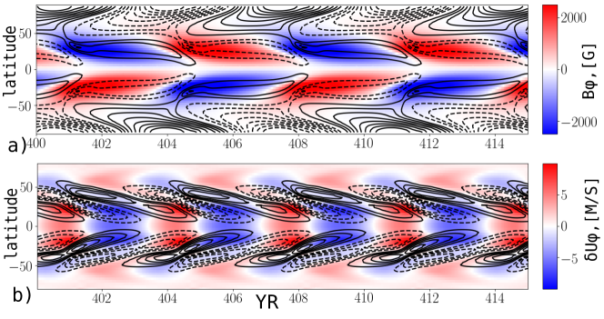
Figure 7: The model M3a4, a) Time-latitude butterfly diagram for the toroidal field in the upper part of the convection zone (color image) and the surface radial magnetic field shown by contours ($\pm$100G); b) the surface variations of the azimuthal velocity (color image) and the meridional velocity (contours in the range of $\pm 3.5$ m/s).

Figure 8 shows snapshots of the global flows distributions in the solar convection zone. In drastic difference to the model M3, the counter-clockwise meridional circulation cell in the upper part of the convection zone is divided into two parts. Also, the stagnation point of the bottom cell is shifted equatorward.

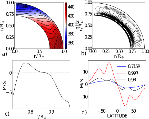
Figure 8: The model M3a4: a) the snapshot of angular velocity profile, $\Omega\left(r,\theta\right)/2\pi$, contours are in range of 347-450 nHz; b) the streamlines of the meridional circulation; c) the radial profile of the meridional flow at $\theta=45^{\circ}$; d) the profiles of the meridional flow at the specific depths of the solar convection zone.

Figure 9 shows the magnetic cycle variations of the global flows in the Northern segment of the solar convection zone for the model M3a4. The patterns of these variations are qualitatively the same as in the model M3. The model M3a4 show the strong magnetic cycle variations of the $\alpha$ effect. Similar to the model M3 we see that the magnetic helicity conservation results into increasing the $\alpha$ -effect in the subsurface shear layer. It occurs just ahead of the dynamo wave drifting toward the top. In the polar regions, the $\alpha$ -effect inverses the sign during inversion of the polar magnetic field. This is different from the model M3 which has the smaller strength of the polar magnetic field than the model M3a4.

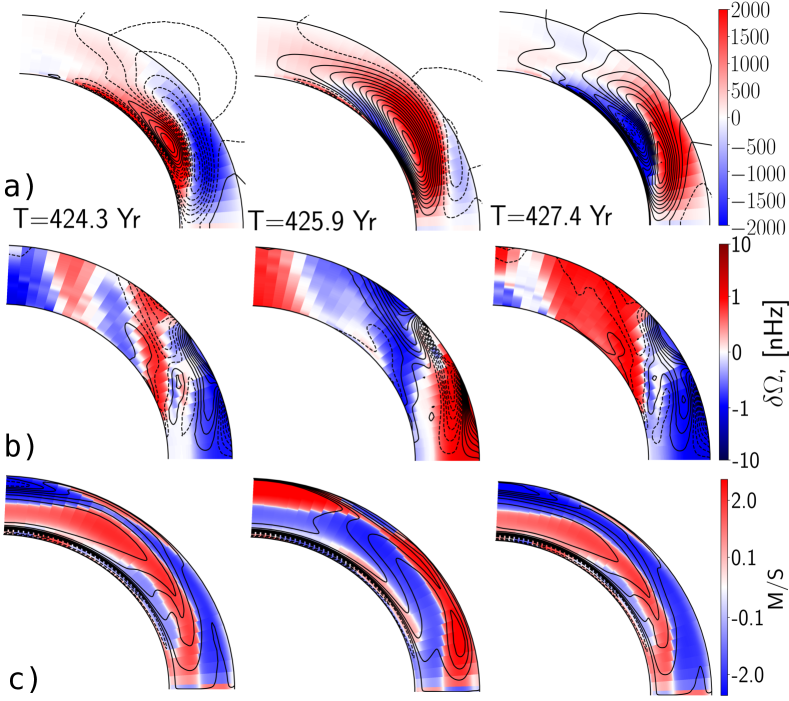
Figure 9: The same as Figure 6 for the model M3a4.

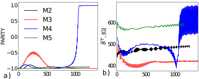
Figure 10: a) Variations of the equatorial symmetry (parity index, see, Eq(19)); b) the same as (a) for the mean density of the toroidal magnetic field flux in the subsurface shear layer. The time series were smoothed to filter out the basic magnetic cycle.

3.3 The long-term dynamo evolution

Figure 10 shows the smoothed time series of evolution of the global properties of the dynamo model, such as the equatorial symmetry index, or the parity index $P$, (see, Eq(19)) and the mean density of the toroidal magnetic field flux, $\overline{B^{T}}$, in the subsurface shear layer, see, Eq(20). In each time series, the basic magnetic cycle was filtered out. The set of models shown in Figure (10) illustrates the effect of variations of magnitude of the eddy-diffusivity of the magnetic helicity density, ${\displaystyle\frac{\eta_{\chi}}{\eta_{T}}}$. From results of Mitra et al. [48], it is expected that ${\displaystyle\frac{\eta_{\chi}}{\eta_{T}}}<1$. In our set of models it is $0.01<{\displaystyle\frac{\eta_{\chi}}{\eta_{T}}}<0.3$. The magnetic helicity diffusion affects the magnetic helicity exchange between hemispheres [3, 48]. Therefore it affects an interaction of the dynamo waves through the solar equator. It is found that the increasing of ${\displaystyle\frac{\eta_{\chi}}{\eta_{T}}}$ results into change of the parity index $P$. The model M4 show the symmetric about equator magnetic field. The magnitude of $\overline{B^{T}}$ in the model M4 is larger than in the models M3 and M5. Both models M3 and M5 operate in a weak nonlinear regime with $0.13<\overline{\beta}<0.24$ (see, Eq(21) and Table(1)). The model M4 has a slightly higher $\overline{\beta}$. This means that the magnetic helicity diffusion affects the strength of the dynamo. This is in agreement with Guerrero et al. [18]. The smoothed time series of $\overline{B^{T}}$ in the model M4 show oscillations at the end of the evolution. This is because the period of the symmetric dynamo mode ( $P=1$) is about 12 years that is larger than the period of the basic magnetic cycle for antisymmetric mode $\left(P=-1\right)$ . The latter is about 10.5 years.

It is interesting to compare the kinematic and nonkinematic dynamo models, which are the models M2 and M3. The nonkinematic model M3 has the smaller parameters $\overline{B^{T}}$and $\overline{\beta}$ than the model M2. Also, it is found that in the kinematic model M2 the stationary phase of evolution is the mix of the dipole-like and quadrupole-like parity, with the mean $P\approx-0.9$. In the model M3 the mean $P\approx-1$. Therefore the nonkinematic dynamo regimes affect the equatorial symmetry of the dynamo solution [7, 59]. Figure 10b shows another interesting difference between the nonlinear kinematic and nonkinematic runs. The kinematic models M2, M4 and M5 show a very slow evolution toward the stationary stage. The given effect was reported earlier by Pipin et al. [70]. The high $R_{m}=10^{6}$ and small diffusivity $\eta_{\chi}$ result to the long time-scale of establishment of the nonlinear balance in magnetic helicity density distributions.

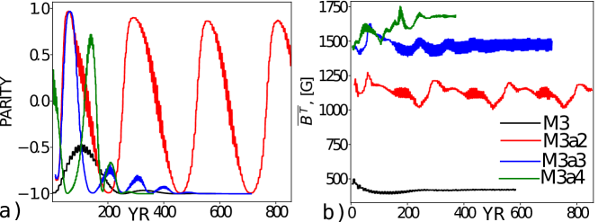
Figure 11: The same as Figure (10) for the models with different $C_{\alpha}$, see Table(1).

Figure (11) shows results for the nonkinematic dynamo models in a range the $\alpha$-effect parameter $C_{\alpha}$. The increasing of the $C_{\alpha}$ results into increasing the nonlinearity of the dynamo model. The parameter $\overline{\beta}$ grows from $0.2$ to $1$ with the increasing of $C_{\alpha}$by factor 4. The model M3a2 shows the long-term periodic variations of the parity index and the magnitude of the toroidal magnetic field $\overline{B^{T}}$. These long-term cycles are likely due to the parity breaking because of the hemispheric magnetic helicity exchange. We made the separate run where the magnetic helicity conservation was ignored and did not find the long-term cycles solution. These cycles are not robust against changes of $C_{\alpha}.$ For the case $\eta_{\chi}=0.1\eta_{T}$, they exist in the range $1.5C_{\alpha}^{(cr)}<C_{\alpha}<3C_{\alpha}^{(cr)}$. The given range is likely to be changed with the change of the magnetic helicity diffusion. We do not consider this case in our paper. Noticeably, that the period of the long-cycle is likely changed with the variation of the $\alpha$-effect. For the model M3a2, the period of the long cycle is about 265 years. In the model M3a3, the establishment of the stationary stage proceeds with the long-term oscillations of about 100 years period. We made the separate runs for the kinematic models with the same $\alpha$-effect and magnetic helicity diffusivity parameters as in the set shown in Figure (11). It was confirmed that the long-term cycles are exists in the range $1.5C_{\alpha}^{(cr)}<C_{\alpha}<3C_{\alpha}^{(cr)}$. Therefore, the magnetic helicity evolution is the most important parameter which governs the long-term periodicity in our model. The magnetic parity breaking and its effect to the Grand activity cycle are lively debated in the literature [7, 79, 40, 16].

3.4 Magnetic cycle in the mean-field heat transport

The global thermodynamic parameters are subjected to the magnetic cycle modulation because of energy loss and gain for the magnetic field generation and dissipation. Also, the magnetic field quenches the magnitude of the convective heat flux. This affects the mean entropy gradient. The Eq(6) takes these processes into account. We remind that in derivation of the mean-field heat transport equation (see, [63]), it was assumed that the magnetic and rotational perturbations of the reference thermodynamic state are small. Also, the basic parameters of the reference state, like $\overline{\rho}$, $\overline{T}$, etc, are given by the reference stellar interior code (MESA). Another approach was suggested recently by Rogachevskii and Kleeorin [76].

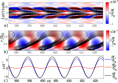
Figure 12: Model M3, a) the time-latitude diagram for the near-surface toroidal magnetic field (contours in range of $\pm 1kG$) and variation of the energy flux on the surface which is calculated relative to the mean background convective flux; b) the same as (a) for the time-radius diagram; c) the mean over the surface outflux of the convective energy (blue line), the magnetic energy and the total energy (black line).

The model calculates the mean entropy variations as an effect of the global flows and magnetic activity. Some results in this direction were previously considered in the dynamo models by Brandenburg et al. [8] and Pipin and Kitchatinov [63]. Figures 12 and 13 show the time-latitude and time-radius diagrams for the magnetic field evolution and variations of the convective heat flux, as well as the mean heat and magnetic energy flux on the surface for the models M3 and M3a4. Evolution of the thermodynamic perturbations goes in form of the cyclic modulations with the double frequency of the magnetic cycle. Like in our previous studies we can identify two major sources of the thermodynamic perturbations in the magnetic cycle. One is the so-called magnetic shadow, which is due to the magnetic quenching of the convective heat flux. This effect is quite small in comparison to the total convective flux. Another effect is the energy expenses on the large-scale dynamo. This contribution is governed by the term ${\displaystyle-\frac{1}{4\pi}\boldsymbol{\mathcal{E}}\cdot\nabla\times\boldsymbol{\overline{B}}}$in the heat transport Eq(6). Note that our boundary conditions (see, Eq(17)), beside the penetration of the toroidal magnetic field to the surface, allow the energy flux from the dynamo region. This flux is related to the strength of the toroidal magnetic field on the surface.

The model M3 shows that the perturbation of the heat energy flux on the surface goes in phase with the evolution of the near-surface toroidal magnetic field. The decreasing of the heat flux corresponds to the increase of the toroidal magnetic field. In the growing phase of the cycle, the thermal energy is expended for the magnetic field generation. The opposite process goes during the declining phase of the magnetic cycle. The magnitude of the thermal flux perturbation is about $10^{-4}$ at the surface and it reaches $10^{-3}$ in the depth of the convection zone. The cyclic perturbations of the mean energy flux on the surface are about $10^{-4}$, which is an order of magnitude smaller than in the solar observations.

The mean Poynting flux on the surface has a maximum order of $10^{-5}$ of the background heat energy flux. This flux represents the magnetic energy input to the stellar corona. It can be considered as a part of energy source for the magnetic cycle variation of the solar X-ray luminosity. The solar observations show that variations the X-ray background flux is the order of $10^{-6}$ [88]. Therefore the magnetic energy flux in the weakly nonlinear model M3 is enough to explain the solar X-ray luminosity variations assuming that all magnetic energy input is transformed into soft X-ray flux energy.

The model M3a4 shows a different evolution of the thermal perturbations in the solar cycle. The growing phase of the magnetic cycle is much shorter than the declining phase. Also, the strength of the magnetic field in the model M3a4 is about factor 3 higher than in the model M3. The effect of the magnetic shadow dominates contributions from the heat energy expenses to the dynamo. In this case, the minima of the thermal energy flux are roughly located in the extremes of the toroidal magnetic field. By this reason, the mean surface heat energy flux reach minimum just after the maximum of the magnetic cycle. The model M3a4 shows the relative variations of the mean energy flux of the order $2\times 10^{-3}$, which is $0.2$ percent of the background heat flux. The strong magnetic feedback of the heat flux in the model M3a4 likely results to the origin of the second near-equatorial meridional circulation cell. We postpone the analysis of this effect to another paper.

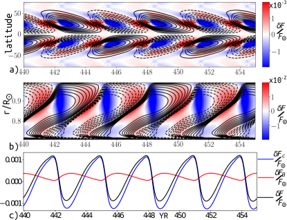
Figure 13: The same as Figure 12 for the model M3a4. The contours of the toroidal magnetic field show the range $\pm 3$kG.

The model M3a4 shows the mean Poynting flux the order of $4\cdot 10^{-4}$. This value is comparable with the X-ray luminosity variations on the young solar analogs, e.g., $\chi^{1}$Ori shows log$L_{x}\sim 29$ [17], which is about $10^{-4}$ of its bolometric luminosity.

4 Discussion and conclusions

The paper presents the new non-kinematic mean-field dynamo model which takes into account the magnetic feedback on the angular momentum and heat transport inside the convection zone. For the first time, the dynamo model takes into account the complicated structure of the meridional circulation cell in the convection zone. In following to [68], the double-cell meridional circulation structure results from inversion of the $\Lambda$-effect sign in the lower part of the convection zone. The similar results are suggested by the helioseismology inversions. Note that the recent results of Chen and Zhao [11] showed the much smaller magnitude of the meridional circulation at the bottom in comparison to the previous results of Zhao et al. [93]. Despite the qualitative similarity of our results with the helioseismology inversions, there are some contradictions. The precise determination of the solar meridional circulation profile remains a matter of the theoretical and observational progress.

The propagation direction of the dynamo wave has been a major problem plaguing distributed turbulent dynamos since helioseismology revealed the solar rotation profile [13, 6, 9]. The issue is further sharpen by uncertainty of the meridional circulation distribution inside the solar convection zone. There is a common misconception in the dynamo community that turbulent dynamos cannot reproduce solar-like activity. Results of Subsection 3.1 show that it is possible to construct the distributed dynamo model with the solar-type magnetic cycles. This requires some tuning of the turbulent pumping coefficients. The required magnitude of the equatorward pumping velocity is about 3 m/s. Also, in the subsurface layer the negative gradient of the angular velocity and the positive sign of the $\alpha$-effect provide the equatorward diffusive drift of the dynamo wave in following to the Parker-Yoshimura law [54, 91]. In addition, the nonlinear models show the increase of the $\alpha$-effect ahead of the dynamo wave, which amplifies the equatorward drift of the toroidal magnetic field, see, the second column of Figures 6 and 9. It was found that the resulted pumping velocity distribution and the effective velocity drift of the large-scale magnetic field are similar to the recent results of direct numerical simulations by Warnecke et al. [85]. For the given choice of the turbulent pumping magnitude, the simulated dynamo wave pattern remains robust in a range of the surface meridional flow variations $\pm 3.5$m/s.

The dynamo model, which is constructed Subsection 3.1, is applied to for the numerical study the effect of the magnetic field on the global flows and heat transport in the solar convection zone. The large-scale magnetic field affects the global flow by means of both the mechanical and thermal effects [74], who showed that, in the presence of the meridional circulation, the “mechanical” perturbations of the angular momentum transport (associated with the large- or small-scale Lorentz force) result in the axial distribution of the torsional oscillation’s magnitude inside the convection zone. This is a consequence of the Taylor-Proudman balance. The results of the helioseismology show deviations of the torsional oscillation from the axial distribution. This was interpreted as results magneto-thermal perturbations. This fact was confirmed in our results. The distribution of magnitude of the zonal flow variations in the subsurface layer declines toward the equator in following the dynamo wave. In the model M3a4 the effect is stronger than in the weakly nonlinear model M3. The proof requires the further analysis like that made in the paper by Guerrero et al. [20]. This is postponed to another paper.

Here, I would like to stress two facts. Firstly, the numerical model suggests the pattern of the torsional oscillation which is in qualitative agreement with observations of Howe et al. [24]. Secondly, the increasing magnetic activity level, for example, due to the $\alpha$ - effect, results in the increasing of the torsional oscillation magnitude and complication of the meridional circulation structure. Comparing the model M3 and M3a4, we find that the stagnation point of the bottom cell is moved to the equator and the upper meridional circulation cell is divided into two cells. The two stagnation points of the upper meridional circulation cell result in to two maxima of the meridional circulation at the surface. There is a similarity between our results and the recent results of Chen and Zhao [11] who also found that the upper circulation cell consists of two. Our model suggest that it may be a result of the strong toroidal magnetic field in the subsurface shear. At the surface, the variations of the meridional circulation in the magnetic cycle show the effective periodical flow towards the maximum of the toroidal magnetic field. In the model M3 the magnitude of this flow is about $\pm 0.5$m/s. The increasing magnetic activity level in the model M3a4 result in the magnitude of the effective flow the order of $\pm 3.5$m/s and the separation into the equatorial and polar meridional circulation cells. A similar effect was also seen in results of Brandenburg et al. [8]. Their model has a different background differential rotation and meridional circulation (one-cell structure) distributions. Note that in the subsurface layer the model M3a4 operates at the sub-equipartition level, $\beta\sim 0.6-1$, which can be confronted with Figure 2b.

The dynamo model shows the decreasing dynamo period with the increasing $\alpha$-effect and the increasing level of the magnetic activity. This is in agreement with results of Pipin and Kosovichev [64] and Pipin et al. [69]. Observations, also, show that, in general, the high solar cycle is shorter than the low solar cycle [80, 21]. Also, the shape of the high cycle is different in compare with the low cycles. This can be deduced in comparison of the time-latitude diagrams of the model M3 and M3a4, for example, in confronting Figures 12a and 13a, we see that in the model M3a4 the growing phase of the dynamo wave is much shorter than the decaying phase. In the model M3, the given asymmetry is less than in the model M3a4. For the first time, we find these relationships (period-amplitude and shape-amplitude) in the mean-field model with the meridional circulation. The flux-transport models fail to explain the relationship between the solar cycle period and cycle amplitude. In particular, the kinematic models of [32] show the increasing dynamo period with the increasing level of the magnetic activity. This contradicts to solar and stellar observations (see, e.g., [52, 14]). On another hand, the distributed dynamo models are well fitted both in the solar and stellar observations. Our current results show that including the meridional circulation in the model does not necessarily result in the increasing magnetic cycle period with the increasing level of magnetic field strength. Therefore the issue of the flux-transport scenario is likely connected with the localized character of the magnetic field generation effects in the dynamo model.

For the first time we demonstrate that the Grand activity cycles can result from effect of the meridional circulation and the equatorial parity breaking because of the hemispheric magnetic helicity exchange. The solar data show that hemispheric magnetic helicity exchange is a real phenomenon [3, 92, 89]. In our model, the process is controlled by diffusion of the magnetic helicity density and by the magnetic helicity transport with the meridional circulation. Mitra et al. [48] found this phenomenon in the direct numerical simulations. In the weakly nonlinear regimes, the strength of the magnetic helicity diffusion affects the parity of solution. We find that the symmetric about equator toroidal magnetic field is generated when the diffusion coefficient is high enough. This is consistent with the observed increase of the $\alpha$-effect ahead of the dynamo wave. The Grand activity cycle regime is not robust and it disappears when $C_{\alpha}>3C_{\alpha}^{(cr)}$. This coincides with the formation of the second meridional circulation cell near the equator. Currently, it is not clear if both phenomena are tightly related or this is an accident. This will be studied further.

We show the first results about effects of the large-scale magnetic activity on the heat transport and the heat energy flux from the dynamo region. This was previously discussed in papers of Brandenburg et al. [8] and Pipin and Kitchatinov [63]. In the mean-field framework, the major contributions of the large-scale magnetic field on the heat energy balance inside the convection zone are caused by the magnetic quenching of the eddy heat conductivity and the energy expenses (associating with the heat energy loss and gain) on the large-scale dynamo. These processes are modeled by the mean-field heat transport equations. The magnetic perturbations of the heat flux in the model M3 are an order of $10^{-3}$ of the background value. It is an order of magnitude less at the surface because of the screening effect and the smaller strength of the large-scale magnetic field in the upper layer of the convection zone. The heat perturbation screening effect is due to the huge heat capacity of the solar convection zone [82]. Results of the model M3a4 illustrate it better than the model M3. The model M3a4 shows the strong toroidal magnetic field in the bulk of the convection zone (see Figure 13b). In the upper layer of the convection zone, the strength of the toroidal field exceeds the equipartition level. Besides this, the heat flux perturbations are efficiently smoothed out toward the top of the dynamo region. Another interesting feature is that the weakly nonlinear model M3 shows the increasing mean heat flux at the maximum of the magnetic cycle. In the model with the overcritical $\alpha$ effect, we find the opposite situation. The solar observations show the increasing luminosity during the maximum of the solar cycles [87]. The variation of the photometric brightness of solar-type stars tends to inverse the sign with the increasing level of the magnetic activity [90]. From the point of view of our model, this means that the effect of the magnetic shadow become dominant when the total magnetic activity is increased. This is a preliminary conclusion. Also, the relationship between the magnetic shadow effect in the large-scale dynamo and the stellar surface darkening because of starspots is not straightforward.

Finally, our results can be summarized as follows:

1. We constructed the nonkinematic solar-type dynamo model with the double-cell meridional circulation. The role of the turbulent pumping in the dynamo model should be investigated. This requires a better theoretical and observational knowledge of the solar meridional circulation.

2. The torsional oscillations are explained as a result of the magnetic feedback on the angular momentum transport by the turbulent stresses, the effect of the Lorentz force and the magneto-thermal perturbations of the Taylor-Proudman balance. The increasing level of the magnetic activity results in separation of the upper meridional circulation cell for two parts.

3. The model shows the decrease of the dynamo period with the increase of the magnetic cycle amplitude. The shape of the strong magnetic cycle is more asymmetric than the shape of the weak cycles.

4. The magnetic helicity density diffusion and the increase turbulent generation of the large-scale magnetic field results in the increasing hemispheric magnetic helicity exchange, the magnetic parity breaking and the Grand activity cycles. The Grand activity cycles exists in the intermediate range of the $\alpha$ - effect parameter, when $1.5C_{\alpha}^{(cr)}<C_{\alpha}<3C_{\alpha}^{(cr)}$. It seems that the Grand activity cycles disappear together with the formation of the second meridional circulation cell near the equator.

5. The increasing turbulent generation of the large-scale magnetic field changes of the relationship between the magnetic cycle phase and the mean sign of the heat flux perturbation at the surface. For the high level of the magnetic activity, the heat flux is reduced in the maximum of the magnetic cycle.

Acknowledgments. This work was conducted as a part of FR II.16 of ISTP SB RAS. Author thanks the financial support from of RFBR grant 17-52-53203.

REFERENCES

Appendix

Heat transport

Pipin [60] found that under the joint action of the Coriolis force and the large-scale toroidal magnetic field, and when it holds $\Omega^{*}>1$, the eddy heat conductivity tensor could be approximated as follows

$$\chi_{ij}\approx\chi_{T}\left(\phi_{\chi}^{(I)}\left(\beta\right)\phi\left(\Omega^{*}\right)\delta_{ij}+\phi_{\chi}^{(\|)}\left(\beta\right)\phi_{\parallel}\left(\Omega^{*}\right)\frac{\Omega_{i}\Omega_{j}}{\Omega^{2}}\right),$$ (25)

where functions $\phi$ and $\phi_{\parallel}$ were defined in Kitchatinov et al. [36], and the magnetic quenching functions $\phi_{\chi}^{(I)}$ and $\phi_{\chi}^{(\|)}$ are

$$\phi_{\chi}^{(I)} = \frac{2}{\beta^{2}}\left(1-\frac{1}{\sqrt{1+\beta^{2}}}\right),$$

$$\phi_{\chi}^{(\|)} = \frac{2}{\beta^{2}}\left(\sqrt{1+\beta^{2}}-1\right).$$

where $\beta=\left|\overline{\mathbf{B}}\right|/\sqrt{4\pi\overline{\rho}u^{\prime 2}}$. The difference of the Eq(25) from results of Kitchatinov et al. [36] is that for $\Omega^{*}\gg 1$ and $\beta\gg 1$ the isotropic and anisotropic part of the eddy heat conductivity tensor become close.

The turbulent stress tensor

Expression of the turbulent stress tensor results from the mean-field hydrodynamics theory (see, [36, 33]) as follows

$${\hat{T}_{ij}=\left(\left\langle u_{i}u_{j}\right\rangle-\frac{1}{4\pi\overline{\rho}}\left(\left\langle b_{i}b_{j}\right\rangle-\frac{1}{2}\delta_{ij}\left\langle\mathbf{b}^{2}\right\rangle\right)\right),}$$ (26)

where $\mathbf{u}$ and $\mathbf{b}$ are fluctuating velocity and magnetic fields. Application the mean-field hydrodynamic framework leads to the Taylor expansion:

$$\hat{T}_{ij} = \hat{T}_{ij}^{\left(\Lambda\right)}+\hat{T}_{ij}^{\left(\nu\right)}$$ (27)

$$= \Lambda_{ijk}\Omega_{k}-N_{ijkl}\frac{\partial\overline{U}_{k}}{\partial r_{l}}+\dots$$ (28)

where the first term represent turbulent generation of the large-scale flow and the second one stands for the dissipative effect. The viscous part of the azimuthal components of the stress tensor is determined following to Kitchatinov et al. [36] in this form:

$${T_{r\phi}^{(\nu)}} {=} -{\nu_{T}\left\{\Phi_{\perp}+\left(\Phi_{\|}-\Phi_{\perp}\right)\mu^{2}\right\}r\frac{\partial\sin\theta\Omega}{\partial r}}$$

$$- {\nu_{T}\sin\theta\left(\Phi_{\|}-\Phi_{\perp}\right)\left(1-\mu^{2}\right)\frac{\partial\Omega}{\partial\mu}}$$

$${T_{\theta\phi}^{(\nu)}} {=} {\nu_{T}\sin^{2}\theta\left\{\Phi_{\perp}+\left(\Phi_{\|}-\Phi_{\perp}\right)\sin^{2}\theta\right\}\frac{\partial\Omega}{\partial\mu}}$$

$$+ {\nu_{T}\left(\Phi_{\|}-\Phi_{\perp}\right)\mu\sin^{2}\theta r\frac{\partial\Omega}{\partial r}},$$

where the eddy viscosity, $\nu_{T}$, is determined from the mixing-length theory assuming the turbulent Prandtl number ${Pr}_{T}={\displaystyle\frac{3}{4}}$:

$$\nu_{T}=\frac{3\ell^{2}}{16}\sqrt{-\frac{g}{2c_{p}}\frac{\partial\overline{{s}}}{\partial r}}.$$

The viscosity quenching functions, $\Phi_{\|}$ and $\Phi_{\perp}$, depend nonlinearly on the Coriolis number, $\Omega^{*}=2\Omega\tau_{c}$, and the strength of the large-scale magnetic field. In the model we employ the analytic expressions for the magnetic quenching functions of the eddy viscosity and the the $\Lambda$- effect obtained by Kitchatinov et al. [36], Kueker et al. [43] and Pipin [59] for the fast rotating regime ($\Omega^{*}>1$):

$${\Phi_{\perp}} {=} \psi_{\perp}\left(\Omega^{\star}\right)\left(\phi_{V\perp}\left(\beta\right)+\phi_{\chi}^{(I)}\left(\beta\right)\right)$$ (31)

$$\Phi_{\parallel} = {\psi_{\parallel}\left(\Omega^{\star}\right)\phi_{\chi}^{(I)}\left(\beta\right),}$$ (32)

where the $\psi_{\perp}$ and $\psi_{\parallel}$ are determined by Kitchatinov et al. [36] and:

$${\phi_{\chi}^{(I)}} {=} {\frac{2}{\beta^{2}}\left(1-\frac{1}{\sqrt{1+\beta^{2}}}\right),}$$ (33)

$${\phi_{V\perp}} {=} {\frac{4}{\beta^{4}\sqrt{\left(1+\beta^{2}\right)^{3}}}\left(\left(\beta^{4}+19\beta^{2}+18\right)\sqrt{\left(1+\beta^{2}\right)}\right.}$$

$$- \left.8\beta^{4}-28\beta^{2}-18\right).$$

The non-diffusive flux of angular momentum $\boldsymbol{\Lambda}=\left\langle{u}_{\phi}^{\prime}{\boldsymbol{u}}\right\rangle$ can be expressed as follows [77]:

$$\hat{T}_{r\phi}^{\left(\Lambda\right)} = r\Lambda_{V}\Omega\sin\theta,$$

$$\Lambda_{V} = \nu_{T}\left(V^{(0)}+\sin^{2}\theta V^{(1)}\right),$$ (35)

$$\hat{T}_{\theta\phi}^{\left(\Lambda\right)} = r\Lambda_{H}\Omega\cos\theta,$$

$$\Lambda_{H} = \nu_{T}\left(H^{(0)}+\sin^{2}\theta H^{(1)}\right)$$ (36)

The basic contributions to the $\Lambda$-effect are due to the density stratification and the Coriolis force [37]. The analytical form of the $\Lambda$-effect coefficients become fairly complicated if we wish to account the multiple-cell meridional circulation structure. In particular, Pipin & Kosovichev (2017) found that the spatial derivative of the Coriolis number $\Omega^{*}=2\Omega_{0}\tau_{c}$, has to be taken into accounted. In nonlinear model we take into account the effect of magnetic field (see, [59]). Also effect of the convective velocities anisotropy is important to account the subsurface shear layer (see, [33]). Therefore, the final coefficients of the $\Lambda$-tensor are:

$$V^{(0)} = \Bigl{[}\left(\frac{\alpha_{MLT}}{\gamma}\right)^{2}\left\{J_{0}+\!J_{1}+\!a\left(I_{0}+\!I_{1}\right)\right\}$$

$$- \Bigl{(}\frac{\alpha_{MLT}\ell}{\gamma}\frac{\partial}{\partial r}\left\{\left(J_{0}+J_{1}\right)-I_{5}+I_{6}\right\}+\ell^{2}\frac{\partial^{2}}{\partial r^{2}}\left(I_{1}-I_{2}\right)\Bigr{]}\phi_{\chi}^{(I)}\left(\beta\right),$$

$$V^{(1)} = -\left\{\left(\frac{\alpha_{MLT}}{\gamma}\right)^{2}\left(J_{1}+aI_{1}\right)-\frac{\alpha_{MLT}\ell}{\gamma}\frac{\partial}{\partial r}\left(J_{1}+I_{6}\right)-\ell^{2}\frac{\partial^{2}}{\partial r^{2}}I_{2}\right\}\phi_{\chi}^{(I)}\left(\beta\right),$$ (38)

and ${H^{(1)}=-V^{(1)}}$. We employ the parameter of the turbulence anisotropy $a={\displaystyle\frac{\overline{u_{h}^{2}}-2\overline{u_{r}^{2}}}{\overline{u_{r}^{2}}}=}2$, where $u_{h}$ and $u_{r}$ are the horizontal and vertical RMS velocities [33]. Collecting results of Kitchatinov et al. [38] and Kueker et al. [43] we write the coefficient $H^{(0)}$ as follows:

$$H^{(0)}=\frac{\tau^{2}}{\rho^{2}}J_{4}\phi_{H}\left(\beta\right)\frac{\partial^{2}}{\partial r^{2}}\left\langle\boldsymbol{u}^{\prime 2}\right\rangle\rho^{2}=\left\{4\left(\frac{\alpha_{MLT}}{\gamma}\right)^{2}J_{4}-\frac{\alpha_{MLT}\ell}{\gamma}\frac{\partial}{\partial r}J_{4}-\ell^{2}\frac{\partial^{2}}{\partial r^{2}}J_{4}\right\}\phi_{H}\left(\beta\right),$$ (39)

where function $J_{4}$ was defined in Kitchatinov et al. [38] and the magnetic quenching function $\phi_{H}\left(\beta\right)$ was defined by Pipin [59]:

$$\phi_{H} = \frac{1}{\beta^{2}}\left(\frac{2+3\beta^{2}}{2\sqrt{\left(1+\beta^{2}\right)^{3}}}-1\right).$$ (40)

Note that $\phi_{H}\approx-\beta^{2}$ for the small magnetic field strength. Therefore the coefficient $H^{(0)}$ disappears in the absence of the large-scale magnetic field. The quenching functions of the the Coriolis number $\Omega^{*}$, $J_{n}$and $I_{n}$were defined in Kitchatinov and Rudiger [37] and Kitchatinov et al. [38]. For convenience, they are given below. Functions $I_{n}$ have the following form:

$$I_{1} = \frac{1}{4\Omega^{*4}}\left(\frac{6+5\Omega^{*2}}{1+\Omega^{*2}}-\left(6+\Omega^{*2}\right)\frac{\arctan\Omega^{*}}{\Omega^{*}}\right),$$

$$I_{2} = \frac{1}{8\Omega^{*4}}\Bigl{(}60+\Omega^{*2}-\frac{6\Omega^{*2}}{1+\Omega^{*2}}$$

$$+ \left(\Omega^{*4}-15\Omega^{*2}-60\right)\frac{\arctan\Omega^{*}}{\Omega^{*}}\Bigr{)},$$

$$I_{3} = \frac{1}{2\Omega^{*4}}\left(-3+\frac{\Omega^{*2}}{1+\Omega^{*2}}+3\frac{\arctan\Omega^{*}}{\Omega^{*}}\right),$$

$$I_{4} = \frac{1}{2\Omega^{*4}}\left(-15+\frac{2\Omega^{*2}}{1+\Omega^{*2}}+\left(15+3\Omega^{*2}\right)\frac{\arctan\Omega^{*}}{\Omega^{*}}\right),$$

$$I_{5} = \frac{1}{2\Omega^{*4}}\left(-3+\left(\Omega^{*2}+3\right)\frac{\arctan\Omega^{*}}{\Omega^{*}}\right),\,I_{6}=\frac{1}{2}I_{4},$$

$$J_{4} = \frac{1}{16\Omega^{*6}}\Bigl{(}40-\frac{31}{3}\Omega^{*2}-3\Omega^{*4}$$

$$- \left(3\Omega^{*6}-10\Omega^{*4}+3\Omega^{*2}+40\right)\frac{\arctan\Omega^{*}}{\Omega^{*}}\Bigr{)}$$

In addition, we have $J_{0}=4I_{1}+2I_{5}$ and $J_{1}=-4I_{2}-2I_{6}$, see the above cited paper.

The first RHS term of Eq.(2.1) describes dissipation of the mean vorticity, $\omega$. It has a combersome expression (see,77):

$$-\left[\boldsymbol{\nabla}\times\frac{1}{\overline{\rho}}\boldsymbol{\nabla\cdot}\overline{\rho}\hat{\mathbf{T}}\right]_{\phi} = \frac{\sin\theta}{r^{2}}\frac{\partial^{2}}{\partial\mu^{2}}\sin\theta\psi_{1}\left(\beta\right)\hat{T}_{r\theta}^{\left(\nu\right)}-\frac{1}{r}\frac{\partial}{\partial r}\frac{1}{r^{2}\overline{\rho}}\frac{\partial}{\partial r}r^{3}\overline{\rho}\psi_{1}\left(\beta\right)\hat{T}_{r\theta}^{\left(\nu\right)}$$ (41)

$$- \frac{1}{r}\frac{\partial}{\partial r}\frac{\partial}{\partial\mu}\sin\theta\psi_{1}\left(\beta\right)\left(\hat{T}_{rr}^{\left(\nu\right)}-\hat{T}_{\theta\theta}^{\left(\nu\right)}\right)+\frac{\cot\theta}{r}\frac{\partial}{\partial r}\psi_{1}\left(\beta\right)\left(\hat{T}_{\phi\phi}^{\left(\nu\right)}-\hat{T}_{rr}^{\left(\nu\right)}\right)$$ (42)

$$+ \frac{\sin\theta}{r^{2}}\frac{\partial}{\partial\mu}\psi_{1}\left(\beta\right)\left(\hat{T}_{\theta\theta}^{\left(\nu\right)}+\hat{T}_{\phi\phi}^{\left(\nu\right)}-2\hat{T}_{rr}^{\left(\nu\right)}\right)-\frac{\sin\theta}{r\overline{\rho}}\frac{\partial\overline{\rho}}{\partial r}\frac{\partial}{\partial\mu}\psi_{1}\left(\beta\right)\hat{T}_{rr}^{\left(\nu\right)}$$ (43)

where, $\mu=\cos\theta$, the components of $\hat{T}_{ij}^{\left(\nu\right)}$ are given in Kitchatinov et al. [36], the magnetic quenching function $\psi_{1}\left(\beta\right)$ (see the above cited paper) takes into account the magnetic feedback on the eddy-viscosity tensor in the simplest way.

The $\alpha$ and $\eta$ tensors

The $\alpha$- effect takes into account the kinetic and magnetic helicities,

$$\alpha_{ij} = C_{\alpha}\psi_{\alpha}(\beta)\alpha_{ij}^{(H)}\eta_{T}+\alpha_{ij}^{(M)}\frac{\overline{\chi}\tau_{c}}{4\pi\overline{\rho}\ell^{2}}$$ (44)

where $C_{\alpha}$ is a free parameter, the $\alpha_{ij}^{(H)}$ and $\alpha_{ij}^{(M)}$ express the kinetic and magnetic helicity coefficients, respectively, $\overline{\chi}$- is the small-scale magnetic helicity, and $\ell$ is the typical length scale of the turbulence. The helicity coefficients have been derived by Pipin [61] (hereafter P08). The $\alpha_{ij}^{(H)}$ reads,

$$\alpha_{ij}^{(H)} = \delta_{ij}\left\{3\left(f_{10}^{(a)}\left(\mathbf{e}\cdot\boldsymbol{\Lambda}^{(\rho)}\right)+f_{11}^{(a)}\left(\mathbf{e}\cdot\boldsymbol{\Lambda}^{(u)}\right)\right)\right\}+$$

$$+ e_{i}e_{j}\left\{3\left(f_{5}^{(a)}\left(\mathbf{e}\cdot\boldsymbol{\Lambda}^{(\rho)}\right)+f_{4}^{(a)}\left(\mathbf{e}\cdot\boldsymbol{\Lambda}^{(u)}\right)\right)\right\}$$

$$+ 3\left\{\left(e_{i}\Lambda_{j}^{(\rho)}+e_{j}\Lambda_{i}^{(\rho)}\right)f_{6}^{(a)}+\left(e_{i}\Lambda_{j}^{(u)}+e_{j}\Lambda_{i}^{(u)}\right)f_{8}^{(a)}\right\},$$

where $\mathbf{e}={\displaystyle\frac{\boldsymbol{\Omega}}{\Omega}},$ $\mathbf{\boldsymbol{\Lambda}}^{(\rho)}=\boldsymbol{\nabla}\log\overline{\rho}$ , $\mathbf{\boldsymbol{\Lambda}}^{(u)}=\boldsymbol{\nabla}\log\left({u^{\prime}}\ell\right)$ and the $\alpha_{ij}^{(M)}$ reads:

$$\alpha_{ij}^{(M)}=2f_{2}^{(a)}\delta_{ij}-2f_{1}^{(a)}e_{i}e_{j},$$ (46)

Functions $f_{n}^{(a)}\left(\Omega^{*}\right)$ were defined by P08. The magnetic quenching function of the hydrodynamical part of $\alpha$-effect is defined by

$$\psi_{\alpha}=\frac{5}{128\beta^{4}}\left(16\beta^{2}-3-3\left(4\beta^{2}-1\right)\frac{\arctan\left(2\beta\right)}{2\beta}\right).$$ (47)

In the notations of P08 :$\psi_{\alpha}=-3/4\phi_{6}^{(a)}$. The dependence of the $\alpha_{ij}^{(H)}$ and $\alpha_{ij}^{(M)}$ tensors on the Coriolis number is defined in following P08:

$$f_{1}^{(a)} = \frac{1}{4\Omega^{*\,2}}\left(\left(\Omega^{*\,2}+3\right)\frac{\arctan\Omega^{*}}{\Omega^{*}}-3\right),$$

$$f_{2}^{(a)} = \frac{1}{4\Omega^{*\,2}}\left(\left(\Omega^{*\,2}+1\right)\frac{\arctan\Omega^{*}}{\Omega^{*}}-1\right),$$

$$f_{4}^{(a)} = \frac{1}{6\Omega^{*\,3}}\left(3\left(\Omega^{*4}+6\varepsilon\Omega^{*2}+10\varepsilon-5\right)\frac{\arctan\Omega^{*}}{\Omega^{*}}\right.$$

$$- \left.\left((8\varepsilon+5)\Omega^{*2}+30\varepsilon-15\right)\right),$$

$$f_{5}^{(a)} = \frac{1}{3\Omega^{*\,3}}\left(3\left(\Omega^{*4}+3\varepsilon\Omega^{*2}+5(\varepsilon-1)\right)\frac{\arctan\Omega^{*}}{\Omega^{*}}\right.$$

$$- \left.\left((4\varepsilon+5)\Omega^{*2}+15(\varepsilon-1)\right)\right),$$

$$f_{6}^{(a)} = -\frac{1}{48\Omega^{*\,3}}\left(3\left(\left(3\varepsilon-11\right)\Omega^{*2}+5\varepsilon-21\right)\frac{\arctan\Omega^{*}}{\Omega^{*}}\right.$$

$$- \left.\left(4\left(\varepsilon-3\right)\Omega^{*2}+15\varepsilon-63\right)\right),$$

$$f_{8}^{(a)} = -\frac{1}{12\Omega^{*\,3}}\left(3\left(\left(3\varepsilon+1\right)\Omega^{*2}+4\varepsilon-2\right)\frac{\arctan\Omega^{*}}{\Omega^{*}}\right.$$

$$- \left.\left(5\left(\varepsilon+1\right)\Omega^{*2}+12\varepsilon-6\right)\right),$$

$$f_{10}^{(a)} = -\frac{1}{3\Omega^{*\,3}}\left(3\left(\Omega^{*2}+1\right)\left(\Omega^{*2}+\varepsilon-1\right)\frac{\arctan\Omega^{*}}{\Omega^{*}}\right.$$

$$- \left.\left(\left(2\varepsilon+1\right)\Omega^{*2}+3\varepsilon-3\right)\right),$$

$$f_{11}^{(a)} = -\frac{1}{6\Omega^{*\,3}}\left(3\left(\Omega^{*2}+1\right)\left(\Omega^{*2}+2\varepsilon-1\right)\frac{\arctan\Omega^{*}}{\Omega^{*}}\right.$$

$$- \left.\left(\left(4\varepsilon+1\right)\Omega^{*2}+6\varepsilon-3\right)\right).$$

Note, that the parameter $\varepsilon={\displaystyle\frac{\overline{\mathbf{b}^{2}}}{\mu_{0}\overline{\rho}\overline{\mathbf{u}^{2}}}}$, control the theoretical ratio between the magnetic and kinetic energies of fluctuations in the background turbulence. It is assumed that $\varepsilon=1$.

We employ the anisotropic diffusion tensor which is derived in P08 and in [67]:

$$\eta_{ijk} = 3\eta_{T}\left\{\left(2f_{1}^{(a)}-f_{2}^{(d)}\right)\varepsilon_{ijk}+2f_{1}^{(a)}\frac{\Omega_{i}\Omega_{n}}{\Omega^{2}}\varepsilon_{jnk}\right\}$$

$$+ a\eta_{T}\phi_{1}\left(g_{n}g_{j}\varepsilon_{ink}-\varepsilon_{ijk}\right)$$

where $\mathbf{g}$ is the unit vector in the radial direction. We employ the same turbulence anisotropy parameter $a=2$ as for the $\Lambda$ effect. The quenching functions $f_{2}^{(d)}$and $\phi_{1}$ are determined in P08 and in Pipin and Kosovichev [67]:

$$f_{2}^{(d)} = \frac{1}{2\Omega^{*\,3}}\left(\left(\varepsilon+1\right)\Omega^{*\,2}+3\varepsilon\right.$$ (49)

$$- \left.\left(\left(2\varepsilon+1\right)\Omega^{*\,2}+3\varepsilon\right)\frac{\arctan\left(\Omega^{*}\right)}{\Omega^{*}}\right)$$ (50)

$$\phi_{1} = -\frac{1}{24\Omega^{\star 2}}\left(2\log\left(1+4\Omega^{\star 2}\right)+4\log\left(1+\Omega^{\star 2}\right)+\right.$$

$$+\left.\left(1-4\Omega^{\star 2}\right)\frac{\arctan\left(2\Omega^{\star}\right)}{\Omega^{\star}}+4\left(1-\Omega^{\star 2}\right)\frac{\arctan\left(\Omega^{\star}\right)}{\Omega^{\star}}-6\right).$$

REFERENCES

- Bekki and Yokoyama [2017] Bekki, Y., Yokoyama, T., Jan. 2017. Double-cell-type Solar Meridional Circulation Based on a Mean-field Hydrodynamic Model. ApJ835, 9.
- Berdyugina [2005] Berdyugina, S. V., Dec. 2005. Starspots: A Key to the Stellar Dynamo. Living Reviews in Solar Physics 2, 8.
- Berger and Ruzmaikin [2000] Berger, M. A., Ruzmaikin, A., May 2000. Rate of helicity production by solar rotation. J. Geophys. Res.105, 10481.
- Bonanno et al. [2002] Bonanno, A., Elstner, D., Rüdiger, G., Belvedere, G., Aug. 2002. Parity properties of an advection-dominated solar alpha2 Omega-dynamo. A & A390, 673.
- Böning et al. [2017] Böning, V. G. A., Roth, M., Jackiewicz, J., Kholikov, S., Aug. 2017. Inversions for Deep Solar Meridional Flow Using Spherical Born Kernels. ApJ845, 2.
- Brandenburg [2005] Brandenburg, A., 2005. The case for a distributed solar dynamo shaped by near-surface shear. Astrophys. J. 625, 539.
- Brandenburg et al. [1989] Brandenburg, A., Krause, F., Meinel, R., Moss, D., Tuominen, I., Apr. 1989. The stability of nonlinear dynamos and the limited role of kinematic growth rates. A & A213, 411.
- Brandenburg et al. [1992] Brandenburg, A., Moss, D., Tuominen, I., Nov. 1992. Stratification and thermodynamics in mean-field dynamos. A & A265, 328.
- Brandenburg and Subramanian [2005] Brandenburg, A., Subramanian, K., Oct. 2005. Astrophysical magnetic fields and nonlinear dynamo theory. Phys. Rep.417, 1.
- Chatterjee et al. [2011] Chatterjee, P., Guerrero, G., Brandenburg, A., Jan. 2011. Magnetic helicity fluxes in interface and flux transport dynamos. A & A525, A5.
- Chen and Zhao [2017] Chen, R., Zhao, J., Nov. 2017. A Comprehensive Method to Measure Solar Meridional Circulation and the Center-to-limb Effect Using Time-Distance Helioseismology. ApJ849, 144.
- Choudhuri and Dikpati [1999] Choudhuri, A. R., Dikpati, M., Jan. 1999. On the large-scale diffuse magnetic field of the Sun - II.The Contribution of Active Regions. Sol.Phys.184, 61.
- Choudhuri et al. [1995] Choudhuri, A. R., Schussler, M., Dikpati, M., Nov. 1995. The solar dynamo with meridional circulation. A & A303, L29.
- Egeland [2017] Egeland, R., 2017. Long-Term Variability of the Sun in the Context of Solar-Analog Stars. Ph.D. thesis.
- Featherstone and Miesch [2015] Featherstone, N. A., Miesch, M. S., May 2015. Meridional Circulation in Solar and Stellar Convection Zones. ApJ804, 67.
- Feynman and Ruzmaikin [2014] Feynman, J., Ruzmaikin, A., Aug. 2014. The Centennial Gleissberg Cycle and its association with extended minima. Journal of Geophysical Research (Space Physics) 119, 6027.
- Gudel et al. [1998] Gudel, M., Guinan, E. F., Skinner, S. L., 1998. The X-Ray and Radio Sun in Time: Coronal Evolution of Solar-Type Stars with Different Ages. In: Donahue, R. A., Bookbinder, J. A. (Eds.), Cool Stars, Stellar Systems, and the Sun. Vol. 154 of Astronomical Society of the Pacific Conference Series. p. 1041.
- Guerrero et al. [2010] Guerrero, G., Chatterjee, P., Brandenburg, A., Dec. 2010. Shear-driven and diffusive helicity fluxes in dynamos. MNRAS 409, 1619.
- Guerrero et al. [2016a] Guerrero, G., Smolarkiewicz, P. K., de Gouveia Dal Pino, E. M., Kosovichev, A. G., Mansour, N. N., Mar. 2016a. On the Role of Tachoclines in Solar and Stellar Dynamos. ApJ819, 104.
- Guerrero et al. [2016b] Guerrero, G., Smolarkiewicz, P. K., de Gouveia Dal Pino, E. M., Kosovichev, A. G., Mansour, N. N., Sep. 2016b. Understanding Solar Torsional Oscillations from Global Dynamo Models. ApJL828, L3.
-
Hathaway [2009]
Hathaway, D., 2009. Solar cycle forecasting. Space Science Reviews 144,
401, 10.1007/s11214-008-9430-4.
URL http://dx.doi.org/10.1007/s11214-008-9430-4 - Hazra et al. [2014] Hazra, G., Karak, B. B., Choudhuri, A. R., Feb. 2014. Is a Deep One-cell Meridional Circulation Essential for the Flux Transport Solar Dynamo? ApJ782, 93.
- Hazra and Nandy [2016] Hazra, S., Nandy, D., Nov. 2016. A Proposed Paradigm for Solar Cycle Dynamics Mediated via Turbulent Pumping of Magnetic Flux in Babcock-Leighton-type Solar Dynamos. ApJ832, 9.
- Howe et al. [2011] Howe, R., Hill, F., Komm, R., Christensen-Dalsgaard, J., Larson, T. P., Schou, J., Thompson, M. J., Ulrich, R., Jan. 2011. The torsional oscillation and the new solar cycle. Journal of Physics Conference Series 271 (1), 012074.
- Hubbard and Brandenburg [2012] Hubbard, A., Brandenburg, A., Mar. 2012. Catastrophic Quenching in Dynamos Revisited. ApJ748, 51.
- Jouve et al. [2008] Jouve, L., Brun, A. S., Arlt, R., Brandenburg, A., Dikpati, M., Bonanno, A., Käpylä, P. J., Moss, D., Rempel, M., Gilman, P., Korpi, M. J., Kosovichev, A. G., Jun. 2008. A solar mean field dynamo benchmark. A & A483, 949.
- Käpylä [2017] Käpylä, P. J., Dec. 2017. Magnetic and rotational quenching of the effect. ArXiv e-prints:1712.08045.
- Käpylä and Brandenburg [2007] Käpylä, P. J., Brandenburg, A., Dec. 2007. Turbulent viscosity and -effect from numerical turbulence models. Astronomische Nachrichten 328, 1006.
- Käpylä et al. [2006] Käpylä, P. J., Korpi, M. J., Ossendrijver, M., Stix, M., Aug. 2006. Magnetoconvection and dynamo coefficients. III. -effect and magnetic pumping in the rapid rotation regime. A & A455, 401.
- Käpylä et al. [2012] Käpylä, P. J., Mantere, M. J., Brandenburg, A., Aug. 2012. Cyclic Magnetic Activity due to Turbulent Convection in Spherical Wedge Geometry. ApJL755, L22.
- Käpylä et al. [2011] Käpylä, P. J., Mantere, M. J., Guerrero, G., Brandenburg, A., Chatterjee, P., Jul. 2011. Reynolds stress and heat flux in spherical shell convection. A & A531, A162.
- Karak et al. [2014] Karak, B. B., Kitchatinov, L. L., Choudhuri, A. R., Aug. 2014. A Dynamo Model of Magnetic Activity in Solar-like Stars with Different Rotational Velocities. ApJ791, 59.
- Kitchatinov [2004] Kitchatinov, L. L., Feb. 2004. Differential Rotation and Meridional Circulation near the Boundaries of the Solar Convection Zone. Astronomy Reports 48, 153.
- Kitchatinov and Olemskoy [2011] Kitchatinov, L. L., Olemskoy, S. V., Feb. 2011. Differential rotation of main-sequence dwarfs and its dynamo efficiency. MNRAS 411, 1059.
- Kitchatinov and Pipin [1993] Kitchatinov, L. L., Pipin, V. V., Jul. 1993. Mean-field buoyancy. A & A274, 647.
- Kitchatinov et al. [1994] Kitchatinov, L. L., Pipin, V. V., Ruediger, G., Feb. 1994. Turbulent viscosity, magnetic diffusivity, and heat conductivity under the influence of rotation and magnetic field. Astronomische Nachrichten 315, 157.
- Kitchatinov and Rudiger [1993] Kitchatinov, L. L., Rudiger, G., Sep. 1993. A-effect and differential rotation in stellar convection zones. A & A276, 96.
- Kitchatinov et al. [1994] Kitchatinov, L. L., Rüdiger, G., Kueker, M., 1994. Lambda-quenching as the nonlinearity in stellar-turbulence dynamos. Astron. Astrophys. 292, 125.
- Kleeorin and Ruzmaikin [1982] Kleeorin, N. I., Ruzmaikin, A. A., 1982. Dynamics of the average turbulent helicity in a magnetic field. Magnetohydrodynamics 18, 116.
- Knobloch et al. [1998] Knobloch, E., Tobias, S. M., Weiss, N. O., Jul. 1998. Modulation and symmetry changes in stellar dynamos. MNRAS297, 1123.
- Kosovichev et al. [1997] Kosovichev, A. G., Schou, J., Scherrer, P. H., Bogart, R. S., Bush, R. I., Hoeksema, J. T., Aloise, J., Bacon, L., Burnette, A., de Forest, C., Giles, P. M., Leibrand, K., Nigam, R., Rubin, M., Scott, K., Williams, S. D., Basu, S., Christensen-Dalsgaard, J., Dappen, W., Rhodes, Jr., E. J., Duvall, Jr., T. L., Howe, R., Thompson, M. J., Gough, D. O., Sekii, T., Toomre, J., Tarbell, T. D., Title, A. M., Mathur, D., Morrison, M., Saba, J. L. R., Wolfson, C. J., Zayer, I., Milford, P. N., 1997. Structure and Rotation of the Solar Interior: Initial Results from the MDI Medium-L Program. Sol.Phys.170, 43.
- Krause and Rädler [1980] Krause, F., Rädler, K.-H., 1980. Mean-Field Magnetohydrodynamics and Dynamo Theory. Berlin: Akademie-Verlag.
- Kueker et al. [1996] Kueker, M., Ruediger, G., Pipin, V. V., Aug. 1996. Solar torsional oscillations due to the magnetic quenching of the Reynolds stress. A & A312, 615.
- Küker et al. [1999] Küker, M., Arlt, R., Rüdiger, G., Mar. 1999. The Maunder minimum as due to magnetic Lambda -quenching. A & A343, 977.
- Labonte and Howard [1982] Labonte, B. J., Howard, R., Jan. 1982. Torsional waves on the sun and the activity cycle. Sol.Phys.75, 161.
- Liu et al. [2007] Liu, Y., Hoeksema, J. T., Zhao, X., Larson, R. M., May 2007. MDI Synoptic Charts of Magnetic Field: Interpolation of Polar Fields. In: American Astronomical Society Meeting Abstracts #210. Vol. 39 of Bulletin of the American Astronomical Society. p. 129.
- Martinez Pillet et al. [1993] Martinez Pillet, V., Moreno-Insertis, F., Vazquez, M., Jul. 1993. The distribution of sunspot decay rates. A & A274, 521.
- Mitra et al. [2010] Mitra, D., Candelaresi, S., Chatterjee, P., Tavakol, R., Brandenburg, A., 2010. Equatorial magnetic helicity flux in simulations with different gauges. Astronomische Nachrichten 331, 130.
- Moss and Brandenburg [1992] Moss, D., Brandenburg, A., Mar. 1992. The influence of boundary conditions on the excitation of disk dynamo modes. A & A256, 371.
- Moss and Brooke [2000] Moss, D., Brooke, J., Jul. 2000. Towards a model for the solar dynamo. MNRAS315, 521.
- Noyes et al. [1984] Noyes, R. W., Weiss, N. O., Vaughan, A. H., Dec. 1984. The relation between stellar rotation rate and activity cycle periods. ApJ287, 769.
- Oláh et al. [2009] Oláh, K., Kolláth, Z., Granzer, T., Strassmeier, K. G., Lanza, A. F., Järvinen, S., Korhonen, H., Baliunas, S. L., Soon, W., Messina, S., Cutispoto, G., Jul. 2009. Multiple and changing cycles of active stars. II. Results. A & A501, 703.
- Parker [1955] Parker, E., 1955. Hydromagnetic dynamo models. Astrophys. J. 122, 293.
- Parker [1955] Parker, E. N., Mar. 1955. The Formation of Sunspots from the Solar Toroidal Field. ApJ121, 491.
- Passos et al. [2017] Passos, D., Miesch, M., Guerrero, G., Charbonneau, P., Feb. 2017. Meridional Circulation Dynamics in a Cyclic Convective Dynamo. ArXiv e-prints.
- Passos et al. [2014] Passos, D., Nandy, D., Hazra, S., Lopes, I., Mar. 2014. A solar dynamo model driven by mean-field alpha and Babcock-Leighton sources: fluctuations, grand-minima-maxima, and hemispheric asymmetry in sunspot cycles. A & A563, A18.
- Paxton et al. [2011] Paxton, B., Bildsten, L., Dotter, A., Herwig, F., Lesaffre, P., Timmes, F., Jan. 2011. Modules for Experiments in Stellar Astrophysics (MESA). ApJS192, 3.
- Paxton et al. [2013] Paxton, B., Cantiello, M., Arras, P., Bildsten, L., Brown, E. F., Dotter, A., Mankovich, C., Montgomery, M. H., Stello, D., Timmes, F. X., Townsend, R., Sep. 2013. Modules for Experiments in Stellar Astrophysics (MESA): Planets, Oscillations, Rotation, and Massive Stars. ApJS208, 4.
- Pipin [1999] Pipin, V. V., Jun. 1999. The Gleissberg cycle by a nonlinear dynamo. A & A346, 295.
- Pipin [2004] Pipin, V. V., 2004. Nonlinear solar dynamo models. Ph.D. thesis, Institute solar-terrestrial physics, Irkutsk, ( Dr Habil Thesis, in Russian).
- Pipin [2008] Pipin, V. V., 2008. The mean electro-motive force and current helicity under the influence of rotation, magnetic field and shear. Geophysical and Astrophysical Fluid Dynamics 102, 21.
- Pipin [2017] Pipin, V. V., Apr. 2017. Non-linear regimes in mean-field full-sphere dynamo. MNRAS466, 3007.
- Pipin and Kitchatinov [2000] Pipin, V. V., Kitchatinov, L. L., Nov. 2000. The Solar Dynamo and Integrated Irradiance Variations in the Course of the 11-Year Cycle. Astronomy Reports 44, 771.
- Pipin and Kosovichev [2011a] Pipin, V. V., Kosovichev, A. G., Nov. 2011a. The Asymmetry of Sunspot Cycles and Waldmeier Relations as a Result of Nonlinear Surface-shear Shaped Dynamo. ApJ 741, 1.
- Pipin and Kosovichev [2011b] Pipin, V. V., Kosovichev, A. G., Feb. 2011b. The Subsurface-shear-shaped Solar Dynamo. ApJL 727, L45.
- Pipin and Kosovichev [2013] Pipin, V. V., Kosovichev, A. G., 2013. The mean-field solar dynamo with a double cell meridional circulation pattern. ApJ776, 36
- Pipin and Kosovichev [2014] Pipin, V. V., Kosovichev, A. G., Apr. 2014. Effects of Anisotropies in Turbulent Magnetic Diffusion in Mean-field Solar Dynamo Models. ApJ785, 49.
- Pipin and Kosovichev [2018] Pipin, V. V., Kosovichev, A. G., Feb. 2018. On the Origin of the Double-cell Meridional Circulation in the Solar Convection Zone. ApJ854, 67.
- Pipin et al. [2012] Pipin, V. V., Sokoloff, D. D., Usoskin, I. G., Jun. 2012. Variations of the solar cycle profile in a solar dynamo with fluctuating dynamo governing parameters. A & A542, A26.
- Pipin et al. [2013a] Pipin, V. V., Sokoloff, D. D., Zhang, H., Kuzanyan, K. M., May 2013a. Helicity Conservation in Nonlinear Mean-field Solar Dynamo. ApJ768, 46.
- Pipin et al. [2013b] Pipin, V. V., Zhang, H., Sokoloff, D. D., Kuzanyan, K. M., Gao, Y., Nov. 2013b. The origin of the helicity hemispheric sign rule reversals in the mean-field solar-type dynamo. MNRAS435, 2581.
- Rajaguru and Antia [2015] Rajaguru, S. P., Antia, H. M., Nov. 2015. Meridional Circulation in the Solar Convection Zone: Time-Distance Helioseismic Inferences from Four Years of HMI/SDO Observations. ApJ813, 114.
- Rempel [2005] Rempel, M., Apr. 2005. Solar Differential Rotation and Meridional Flow: The Role of a Subadiabatic Tachocline for the Taylor-Proudman Balance. ApJ622, 1320.
- Rempel [2006] Rempel, M., Aug. 2006. Flux-Transport Dynamos with Lorentz Force Feedback on Differential Rotation and Meridional Flow: Saturation Mechanism and Torsional Oscillations. ApJ647, 662.
- Roberts and Soward [1975] Roberts, P., Soward, A., 1975. A unified approach to mean field electrodynamics. Astron. Nachr. 296, 49.
- Rogachevskii and Kleeorin [2015] Rogachevskii, I., Kleeorin, N., Oct. 2015. Turbulent fluxes of entropy and internal energy in temperature stratified flows. Journal of Plasma Physics 81 (5), 395810504.
- Ruediger [1989] Ruediger, G., 1989. Differential rotation and stellar convection. Sun and the solar stars, Academie-Verlag, Berlin.
- See et al. [2016] See, V., Jardine, M., Vidotto, A. A., Donati, J.-F., Boro Saikia, S., Bouvier, J., Fares, R., Folsom, C. P., Gregory, S. G., Hussain, G., Jeffers, S. V., Marsden, S. C., Morin, J., Moutou, C., do Nascimento, J. D., Petit, P., Waite, I. A., Nov. 2016. The connection between stellar activity cycles and magnetic field topology. MNRAS462, 4442.
- Sokoloff and Nesme-Ribes [1994] Sokoloff, D., Nesme-Ribes, E., Aug. 1994. The Maunder minimum: A mixed-parity dynamo mode? A & A288, 293.
- Soon et al. [1993] Soon, W. H., Baliunas, S. L., Zhang, Q., Sep. 1993. An interpretation of cycle periods of stellar chromospheric activity. ApJL414, L33.
- Stenflo [2013] Stenflo, J. O., Sep. 2013. Solar magnetic fields as revealed by Stokes polarimetry. Astron. & Astrophys. Rev.21, 66.
- Stix [2002] Stix, M., 2002. The sun: an introduction, 2nd Edition. Berlin : Springer.
- Tobias [1998] Tobias, S. M., May 1998. Relating stellar cycle periods to dynamo calculations. MNRAS296, 653.
- Warnecke et al. [2016] Warnecke, J., Käpylä, P. J., Käpylä, M. J., Brandenburg, A., Dec. 2016. Influence of a coronal envelope as a free boundary to global convective dynamo simulations. A & A596, A115.
- Warnecke et al. [2018] Warnecke, J., Rheinhardt, M., Tuomisto, S., Käpylä, P. J., Käpylä, M. J., Brandenburg, A., Jan. 2018. Turbulent transport coefficients in spherical wedge dynamo simulations of solar-like stars. A & A609, A51.
- Weiss and Tobias [2016] Weiss, N. O., Tobias, S. M., Mar. 2016. Supermodulation of the Sun’s magnetic activity: the effects of symmetry changes. MNRAS456, 2654.
- Willson and Mordvinov [1999] Willson, R. C., Mordvinov, A. V., 1999. Time-frequency analysis of total solar irradiance variations. Geophys. Res. Letter26, 3613.
- Winter and Balasubramaniam [2014] Winter, L. M., Balasubramaniam, K. S., Oct. 2014. Estimate of Solar Maximum Using the 1-8 Å Geostationary Operational Environmental Satellites X-Ray Measurements. ApJL793, L45.
- Yang and Zhang [2012] Yang, S., Zhang, H., Oct. 2012. Large-scale Magnetic Helicity Fluxes Estimated from MDI Magnetic Synoptic Charts over the Solar Cycle 23. ApJ758, 61.
- Yeo et al. [2016] Yeo, K. L., Shapiro, A. I., Krivova, N. A., Solanki, S. K., Apr. 2016. Modelling Solar and Stellar Brightness Variabilities. In: Dorotovic, I., Fischer, C. E., Temmer, M. (Eds.), Coimbra Solar Physics Meeting: Ground-based Solar Observations in the Space Instrumentation Era. Vol. 504 of Astronomical Society of the Pacific Conference Series. p. 273.
- Yoshimura [1975] Yoshimura, H., Nov. 1975. Solar-cycle dynamo wave propagation. ApJ201, 740.
- Zhang et al. [2010] Zhang, H., Yang, S., Gao, Y., Su, J., Sokoloff, D. D., Kuzanyan, K., Aug. 2010. Large-scale Soft X-ray Loops and Their Magnetic Chirality in Both Hemispheres. ApJ719, 1955.
- Zhao et al. [2013] Zhao, J., Bogart, R. S., Kosovichev, A. G., Duvall, Jr., T. L., Hartlep, T., Sep. 2013. Detection of Equatorward Meridional Flow and Evidence of Double-cell Meridional Circulation inside the Sun. ApJL774, L29.
- Zhao et al. [2014] Zhao, J., Kosovichev, A. G., Bogart, R. S., Jul. 2014. Solar Meridional Flow in the Shallow Interior during the Rising Phase of Cycle 24. ApJL789, L7.