REST: Real-to-Synthetic Transform for Illumination Invariant
Camera Localization

Abstract

Accurate camera localization is an essential part of tracking systems. However, localization results are greatly affected by illumination. Including data collected under various lighting conditions can improve the robustness of the localization algorithm to lighting variation. However, this is very tedious and time consuming. By using synthesized images it is possible to easily accumulate a large variety of views under varying illumination and weather conditions. Despite continuously improving processing power and rendering algorithms, synthesized images do not perfectly match real images of the same scene, i.e. there exists a gap between real and synthesized images that also affects the accuracy of camera localization. To reduce the impact of this gap, we introduce “REal-to-Synthetic Transform (REST).” REST is an autoencoder-like network that converts real features to their synthetic counterpart. The converted features can then be matched against the accumulated database for robust camera localization. In our experiments REST improved feature matching accuracy under variable lighting conditions by approximately 30%. Moreover, our system outperforms state of the art CNN-based camera localization methods trained with synthetic images. We believe our method could be used to initialize local tracking and to simplify data accumulation for lighting robust localization.

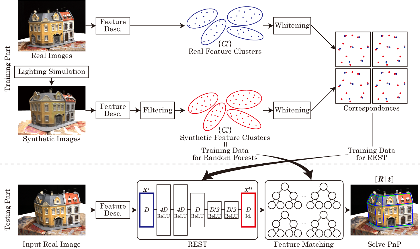
Figure 1: Pipeline of our camera localization system. In the training part, lighting simulation generates synthetic images. The correspondences between features extracted from synthetic images and 3D points are obtained by ray trancing. As shown in the center, each 3D point forms synthetic feature cluster and they are used as training data for random forests. Then, real features are also described to obtain the training data for REST. We group real and synthetic features corresponding to the same 3D points and create feature clusters. To overlap real and synthetic feature clusters which correspond the same 3D point, whitening is applied to the both. The correspondences between a real and synthetic features are used to train REST. In the testing part, REST transforms input real features to synthetic features. Then, the transformed features are matched with accumulated synthetic features in the database. Finally, PnP problem is solved to obtain the camera pose.

1 Introduction

Camera localization is an important task in computer vision. Over the years a variety of approaches that use features extracted from the scene [16, 29], or neural networks [11, 30] have been developed to address it. Both approaches require a large number of images that cover the expected scene appearance to recover a representation of the scene. However, as the appearance varies during the seasons, different weather, as well as different time of the day, it is difficult and time-consuming to acquire a database that covers a sufficient variety of appearances. A cost-efficient solution is to generate synthetic views of the scene instead. Although synthetic image databases offer a lot of flexibility in deciding scene parameters, such as time of the day, weather conditions, or occluders, the synthetic scene will rarely match the appearance of the scene when captured by a camera. This is in part because it is difficult to obtain accurate geometric and optical properties for all objects in the scene. This difference inevitably leads to feature matching failure and decreased localization accuracy [21].

This problem also applies to neural nets trained on synthetic image databases. We show in this paper that a state-of-the-art CNN-based localization algorithm (PoseNet [11]) trained on synthetic images successfully localizes synthetic views of the scene, but fails to localize actual images of the same scene.

In this paper, we introduce an autoencoder-like network “REal-to-Synthetic Transform (REST)” to overcome the “gap” between real images and synthetic images for feature-based localization. REST transforms a feature descriptor extracted from an input image (we refer to it as “real feature”) into a corresponding feature descriptor, if it were extracted from synthetic image (we refer to it as “synthetic feature”) that was generated under the same conditions, i.e. 3D points and lighting conditions, as the real image. After REST transforms a real feature it closely resembles the corresponding synthetic feature, thus increasing the accuracy of matching it with the feature database.

REST can be trained with a small number of real images, and corresponding synthetic views. That is because we do not learn how to accurately estimate the pose of the camera under varying lighting conditions, but the relationship between an extracted real feature and its corresponding synthetic feature. We evaluate our method using images from the DTU robot image dataset [7] that stores image of the same model taken under different lighting conditions within a 1 m $\times$ 1 m area. In this paper, we use only 48 images to train the network and achieve an accuracy of 1.66 cm and 1.41^∘.

Our main contributions are the following.

• We introduce REST to improve matching of real features and a database of synthetic features.

• We show that even when trained on a small number of images REST improves localization accuracy compared to state-of-the-art methods trained only on synthetic images.

• We show that REST is robust to illumination changes and its performance with different feature descriptors.

2 Related Work

Over work focuses on camera localization from synthetic images. In this section we review existing methods on localization and discuss how they utilized synthetic images. Camera localization methods [16, 29, 11, 21, 18, 27, 23, 12, 4, 3, 10, 34] can be divided into feature-based methods and convolutional neural network (CNN)-based methods. We discuss each category as follow.

Feature-based Camera Localization.

Feature-based methods [16, 29, 21, 18, 27] detect 3D points stored in a database in the camera image and estimate the camera pose by solving the perspective $n$-point problem [5]. To detect a 3D point in the image these methods extract a feature descriptor for the detected feature (corner, blob, etc.) in the camera image and for each 3D point match it with the corresponding descriptor stored in the database. When a good match is detected the 2D feature is matched to the corresponding 3D point. Over the years, a variety of descriptors, e.g. SIFT [19], SURF [1], ORB [26] and LIFT [35], that are robust to constrained viewpoint changes have been developed. Storing descriptors for all possible 3D points is not viable, as many features can be discovered only under certain conditions, it leads to a very large database and consequently very long processing time.

Feature databases can be obtained through Structure-from-Motion reconstruction [20], Simultaneous Localization and Mapping methods [23, 12, 4, 3, 22, 32], geo-annotated image datasets [25], or 3D scans of the environment [16, 17]. As all of these methods reconstruct the scene appearance at a particular point in time, they are not robust to drastic changes in lighting conditions. To account for these changes, the database must be generated multiple times under different conditions.

A large database often contains a number of redundant, rarely seen features, many similar features, and multiple descriptors for the same feature. To reduce the size of the database a “representative subset” can be used to ensure good localization results [16, 18]. A subset contains a particular number of the most representative descriptors. These descriptors are either selected based on feature visibility in different views, or descriptor matching robustness. By removing redundant feature descriptors, and reducing the number of overall features in the database these subsets reduce the time required for localization, and improve the robustness of the matching. Feature matching robustness can also be improved by taking advantage of the various sensors embedded into mobile devices [16, 29]. Different methods [29, 21, 27] also utilize synthetic images for viewpoint invariant camera localization.

CNN-based Camera Localization.

CNNs have been deployed for many tasks in computer vision, especially image classification [14, 31]. With the increasing number of available images in various databases, localization with CNNs has gained a lot of attention recently [11, 10, 34]. As these methods require many images with known camera pose, some systems use synthetic data to estimate viewpoints [30] and to predict 6D object poses [15]. To overcome the gap between synthetic and real images, synthetic images can be post-processed with a generative adversarial network (GAN) to change their appearance to more closely resemble that of real images [28]. However, training a GAN requires between 10K and 100K image pairs. It is thus difficult to obtain sufficient number images of the scene under varying lighting conditions to train a GAN.

3 Real-to-Synthetic Feature Transform

Figure 1 shows an overview of our camera localization system. Our goal is to estimate the camera pose $[\bm{R}|\bm{t}]$, where $\bm{R}$ is a rotation matrix and $\bm{t}$ is a translation vector, from a single input RGB image.

We generate synthetic images that simulate a large variety of lighting conditions. Afterward, features will be extracted from these synthetic views and compute the corresponding 3D location from known camera parameters and scene model. For each features we store the computed 3D location and descriptor in a database.

To estimate the pose of an input image, we detect real features $\bm{x}^{\mathrm{r}}$ and match them with our database of synthetic features $\bm{x}^{\mathrm{s}}$. From the matched 2D-3D points, we compute the camera pose with the perspective $n$-point (PnP) algorithm [5]. If the number of correct matches is too small, due to the gap between descriptors acquired from real and synthetic images, the pose estimation fails to recover the correct pose.

Given identical light conditions, the gap between real and synthetic features is due to incorrect assumptions about the geometry and optical properties of the scene. We explain how to overcome these inaccuracy in this section.

3.1 Synthetic-to-Real vs. Real-to-Synthetic

As discussed in the Sec. 1, utilizing image synthesis is a solution for the scene variation problem however we need feature transform between synthetic and real feature. There are two possible ways of feature transform which are real-to-synthetic and synthetic-to-real respectively. An obvious difference between real and synthetic scene is in their complexity. Generally, a real scene is very complex and vary with a number of factors. Moreover, some of the factors are difficult to measure, estimate, and/or synthesize. In other words, a synthetic scene is a simplification of the original real scene (i.e. a subset of real scene). Therefore, synthetic-to-real transform needs latent variables to supplement the difference in complexity. SimGAN [28] does not use latent variables which shows a potential of synthetic-to-real transform. However, this method requires a large amount of real images and learning of a large network for representing complex real scene.

On the other hand, real-to-synthetic transform can be achieved with a simpler network because it is a simplification of the real scene and does not require latent variables. We therefore adopt real-to-synthetic transform as our camera localization. Moreover, our real-to-synthetic transform, REST, is learned with small number of real images.

We hereby execute real-to-synthetic feature transform with an autoencoder-like network REST to overcome the gap between real and synthetic information. Autoencoders have been used for dimension compression [6], pre-training of deep neural networks and denoising [33]. We consider the gap between real and synthetic features to be due to noise and train REST to minimize the loss function

$$L(\bm{x}^{\mathrm{ts}})=\left\|\bm{x}^{\mathrm{ts}}-{\bm{x}^{\mathrm{s}}}\right\|,$$ (1)

where $\bm{x}^{\mathrm{ts}}$ is the real feature $\bm{x}^{\mathrm{r}}$ transformed with REST, and ${\bm{x}^{\mathrm{s}}}$ is the corresponding ground truth synthetic feature. To train REST efficiently, we pre-train REST to transform a synthetic feature into itself before the main training with correspondences between real and synthetic features.

One of the disadvantages of REST is in expansion of map and database. To apply REST to expanded a map and a database, REST must be learned from scratch. In the case of synthetic-to-real transform, theoretically its expandability is higher because new feature can be directly accumulated to the database.

3.2 Correspondences between Real and Synthetic Features

To train REST, correspondence between real and synthetic features are required. Ideally the correspondences between real and synthetic feature both of which are under the same lighting condition are the best, but this is difficult as discussed above. However, by using projection matrices, the correspondence between a set of real features and a set of synthetic features both of which correspond the same 3D point. We use the set correspondences to obtain the feature correspondences. Hereby, we assume that some real images $\{I_{n}\}_{n=1}^{\mathrm{N}}$ and their corresponding projection matrices $\{\bm{P}_{n}\}_{n=1}^{\mathrm{N}}$ are known, where $\mathrm{N}$ represents the number of real images for training. The making of correspondences is separated to three steps below.

First, we compute 3D points for each real and synthetic features. 3D points of synthetic features can be computed by ray casting because we know the camera parameters used in a simulation. Let $\mathcal{V}$ denotes the set of the 3D points of synthetic features. Then, a 3D point of a real feature $\bm{x}^{\mathrm{r}}$, which is extracted from a real image $\mathrm{I}_{n}$, are searched from $\mathcal{V}$ by

$$\bm{v}=\mathop{\rm argmin}\limits_{\bm{v}^{\prime}\in\mathcal{V}}\left\|\pi\left(\bm{P}_{n}\dot{\bm{v}}^{\prime}\right)-\bm{u}\right\|,$$ (2)

where $\pi$ represents perspective projection function defined by

$$\pi\left(\left[x,y,\lambda\right]\right)=\left[\frac{x}{\lambda},\frac{y}{\lambda}\right],$$ (3)

$\dot{\bm{v}}^{\prime}$ represents a homogeneous vector of $\bm{v}^{\prime}$ and $\bm{u}$ represents image points of the real feature $\bm{x}^{\mathrm{r}}$.

Secondly, we group each features by 3D points. We call the group of real features corresponding to a 3D point $\bm{v}$ “real feature cluster” denoted by $C^{\mathrm{r}}_{\bm{v}}$ and call the group of synthetic features corresponding to a 3D point $\bm{v}$ “synthetic feature cluster” denoted by $C^{\mathrm{s}}_{\bm{v}}$. We match $C^{\mathrm{r}}_{\bm{v}}$ with $C^{\mathrm{s}}_{\bm{v}}$.

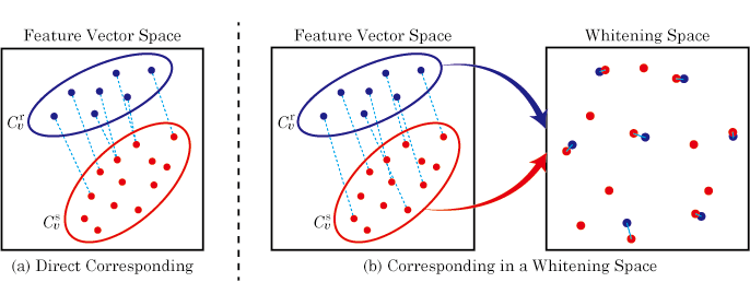
Figure 2: Corresponding between $\bm{x}^{\mathrm{r}}$ in $C^{\mathrm{r}}_{\bm{v}}$ and $\bm{x}^{\mathrm{s}}$ in $C^{\mathrm{s}}_{\bm{v}}$. Red and blue dots represents real features and synthetic features respectively. Each ellipses represents a cluster.

Finally, we make correspondences between a real feature $\bm{x}^{\mathrm{r}}\in C^{\mathrm{r}}_{\bm{v}}$ and a synthetic feature $\bm{x}^{\mathrm{s}}\in C^{\mathrm{s}}_{\bm{v}}$. Since the distribution of a real feature cluster in the feature vector space and that of a synthetic feature cluster in the feature vector space are expected to be different, e.g. shifted or scaled. If we directly correspond a $\bm{x}^{\mathrm{r}}$ with a $\bm{x}^{\mathrm{s}}$ in $C^{\mathrm{s}}_{\bm{v}}$ under a positional relationship like Fig. 2(a), most of $\bm{x}^{\mathrm{r}}$ will be corresponded with $\bm{x}^{\mathrm{s}}$ located in boundary side of the $C^{\mathrm{s}}_{\bm{v}}$. As a result of the learning with this correspondences, $\bm{x}^{\mathrm{r}}$ will be transformed to a position close to the boundary with another cluster and it will increase failure matching. To make better correspondences between a real and synthetic feature, we apply whitening transformation [13] to both of a real and a synthetic feature cluster as shown in Fig. 2(b). Since whitening changes the mean into zero and the variance into one, in the whitening space two clusters are overlapped. Then, we deploy nearest neighbor in the whitened space to obtain the correspondences between a real feature and a synthetic feature.

3.3 Preparation of Training Data for REST

As stated in Sec. 3.2, we can obtain correspondences between real and synthetic features, but this is not enough to train REST because the number of real features are smaller than that of synthetic features. Small number of training data cannot train REST enough. Additionally they cause to transform a real feature into a outlier, which decreases the accuracy of feature matching. Thus the data augmentation is required.

For the preparation of the sufficient training data, we leverage $k$-nearest-neighbor ($k$-NN) in order to increase the number of correspondences between a real and synthetic feature for training data because we use a small number of real images for training, i.e. the number of real features extracted from them is less than that of synthetic features. Moreover, since we train REST with $k$ correspondences $(\bm{x}^{\mathrm{r}},\bm{x}^{\mathrm{s}}_{1}),\cdots,(\bm{x}^{\mathrm{r}},\bm{x}^{\mathrm{s}}_{k})$ per a real feature $\bm{x}^{\mathrm{r}}$ and we use mean square error defined by Eq. (1) as the loss function, $\bm{x}^{\mathrm{r}}$ is transformed to the mean of $\{\bm{x}^{\mathrm{s}}_{1},\cdots,\bm{x}^{\mathrm{s}}_{k}\}$. This means that $\bm{x}^{\mathrm{r}}$ transformed more far from the boundaries of the corresponding synthetic cluster. As we stated in Sec. 3.2, if a real feature is transformed into near the boundaries, it will be possible to cause matching failure.

Additionally, using $k$-NN enables to train REST effectively. We have representative features in a database. Since representative features [18] are robust to camera viewpoint and rotation, the more synthetic features a synthetic cluster has, the more robust to camera viewpoint and rotation such synthetic features are. Therefore focusing on training to transform a real feature into such a synthetic feature improves feature matching accuracy. To focus on such training, we optimize the $k$ value by

$$k=\left\lfloor\gamma\sqrt{|C^{\mathrm{s}}_{\bm{v}}|}\right\rfloor,$$ (4)

where $\gamma$ denotes a parameter to adjust $k$ and $|C^{\mathrm{s}}_{\bm{v}}|$ denotes the number of synthetic features which $C^{\mathrm{s}}_{\bm{v}}$ contains.

4 Implementation

In this section, we illustrate our lighting robust camera localization system. Our system consists of a training and testing part shown in Fig. 1. Training includes the following steps:

1. Generate synthetic images under various lighting conditions. We explain the details in Sec. 4.1.

2. Extract synthetic features from these images and select a representative subset as described in [18].

3. To prepare the training data of REST, we extract real features from some real images, make real and synthetic feature clusters, and find correspondence between real and synthetic features as stated in Sec. 3.2. Moreover we utilize $k$-NN to augment the training data as stated in Sec. 3.3. We empirically set the parameter $\gamma$ in Eq. (4) to 0.2.

4. Train REST that transforms extracted features $\bm{x}^{\mathrm{r}}$ to $\bm{x}^{\mathrm{ts}}$ using the loss function Eq. (1).

5. Train a random forest that matches a transformed feature $\bm{x}^{\mathrm{ts}}$ with the database.

In the testing part,

1. Extract real features $\bm{x}^{\mathrm{r}}$ from the input image.

2. Transform $\bm{x}^{\mathrm{r}}$ into $\bm{x}^{\mathrm{ts}}$ by REST.

3. Match $\bm{x}^{\mathrm{ts}}$ with the database by the trained random forest.

4. Solve PnP problem using random sample consensus (RANSAC) to obtain the camera pose.

4.1 Simulation under Various Lighting Conditions

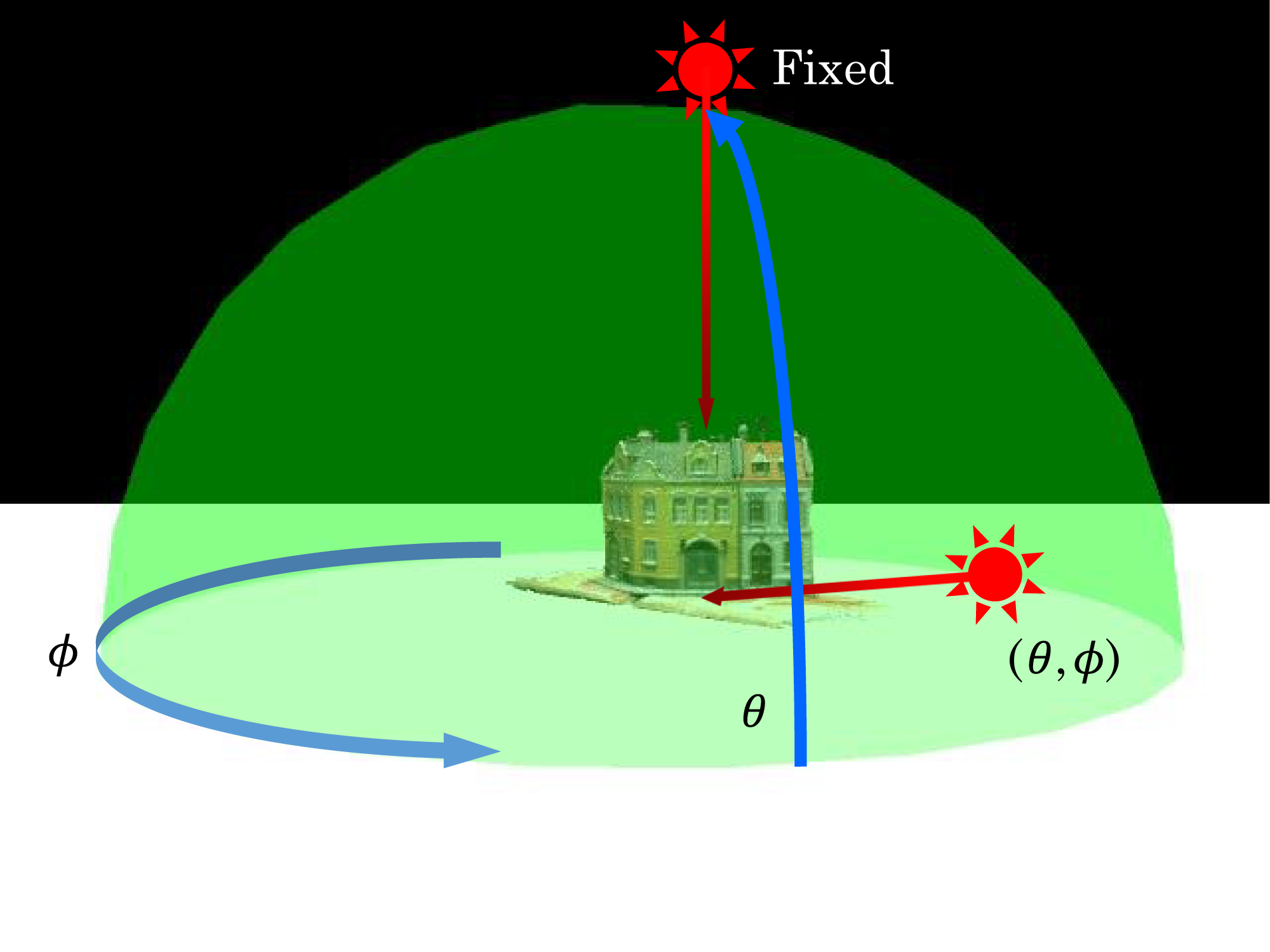
Figure 3: Light sources used in illumination simulation.

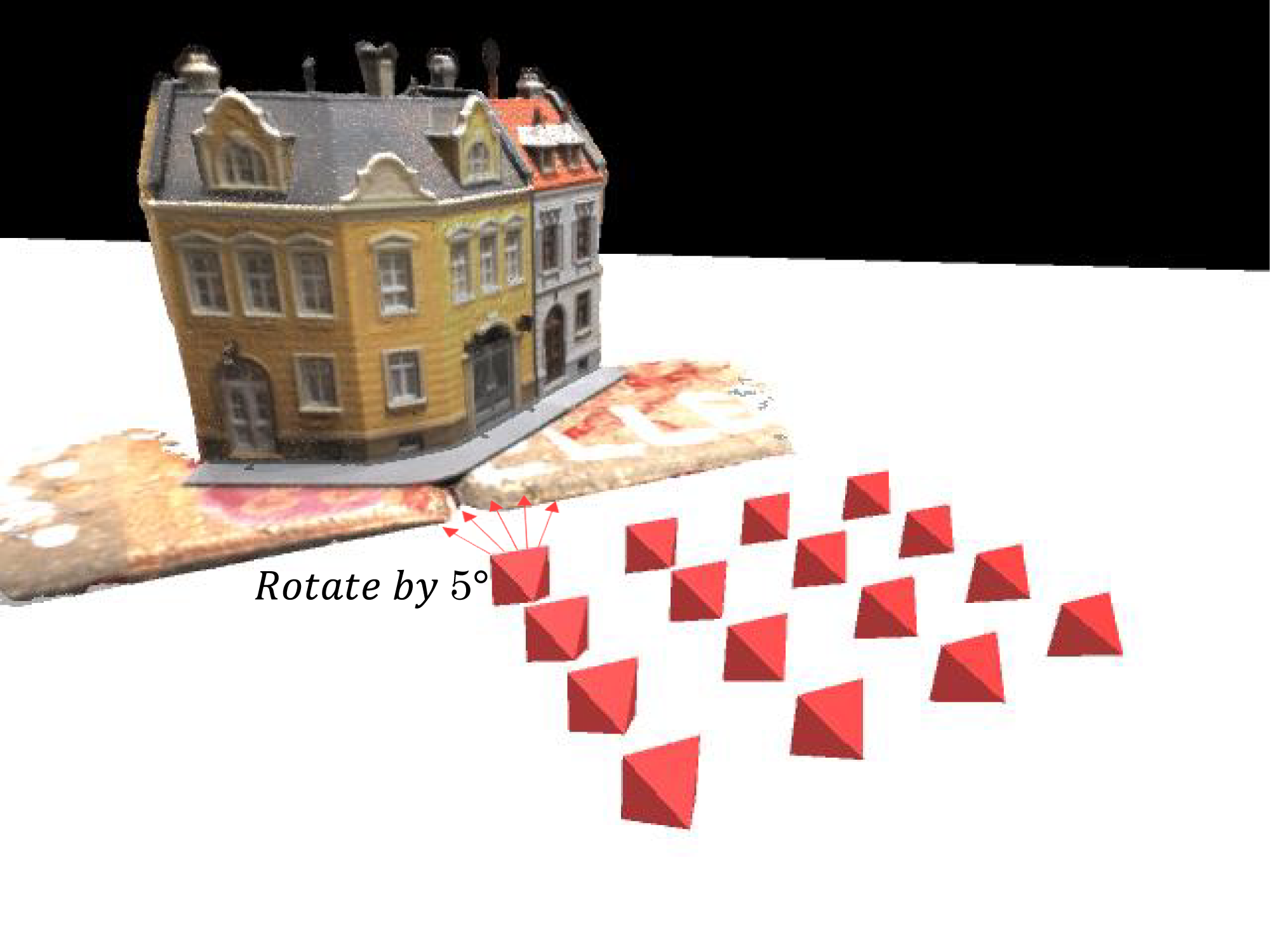
Figure 4: Camera positions for generating synthetic images.

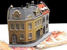
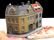
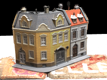
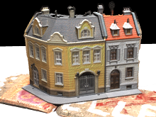
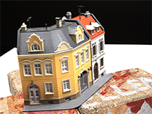
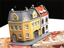
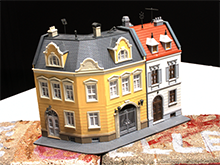
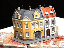
Figure 5: Rendered synthetic images (top) and real images (bottom).

To simulate the scene appearance under varying lighting conditions, we require a 3D model which can be obtained through several approaches such as structure from motion, dense tracking and mapping (DTAM) [24], dense environment scans [16, 17], or Poisson surface reconstruction [8, 2, 9]. In this paper we use the DTU robot image dataset [7]. This dataset contains a structure-from-motion model, real images taken under different lighting conditions, and corresponding projection matrices. We obtain a mesh model through Poisson surface reconstruction of the structure-from-motion model.

To match the illumination conditions in the DTU dataset, we use two parallel light sources. As presented in Fig. 5, one light source illuminates the scene from above, while the other is moved around the scene and always oriented towards the model, as in [7]. The direction the light is coming from is represented by latitude angle $\theta$ and longitude angle $\phi$. $\theta$ is set to $\{10,20,30,\cdots,80\}$ and $\phi$ is set to $\{0,30,60,\cdots,180\}$ degrees, i.e. we simulate 56 lighting conditions in total.

We generate views of the scene from $4\times 4$ positions in front of the model (shown in Fig. 5) and rotate the camera from 170^∘ to 190^∘ in 5^∘ steps. The positions were chosen to simulate the system being used by pedestrians. Overall, we generate 80 images per lighting condition, i.e. 4,480 synthetic images in total. We show examples of the rendered images in Fig. 5.

4.2 Training Random Forest

For feature matching, we use random forests because it is used for feature matching and training simplicity. The random forest classifies a synthetic feature transformed by REST into its corresponding to synthetic feature cluster. Since synthetic feature clusters are related with a scene coordinate, correspondences between a image coordinate and a scene coordinate can be obtained.

However, random forest can mismatch a synthetic feature which is corresponding to non-synthetic feature clusters, i.e. a noise feature, with one of the feature clusters. To remove mismatches and reduce the time which RANSAC takes, we apply filtering before executing RANSAC. A random forest estimates probabilities which input values are classified to a class. We ordered all matches by maximum probabilities, i.e. the probabilities the feature is matched with the predicted synthetic feature clusters, and select the top 100 matches as an input to RANSAC.

5 Evaluation

Table 1: Result of evaluation for REST. From left column, matching accuracy (MA), position error (PE), orientation error (OE), and localization time are indicated.

			$\mathrm{MA}$	$\mathrm{PE}$	$\mathrm{OE}$	$\mathrm{Time}$
SIFT	naïve method	mean	$47.77\%$	$19.75\ \mathrm{cm}$	$26.01^{\circ}$	$373.12\ \mathrm{ms}$
		median	$57.58\%$	$3.47\ \mathrm{cm}$	$2.84^{\circ}$	$375.79\ \mathrm{ms}$
	REST	mean	$58.81\%$	$30.09\ \mathrm{cm}$	$34.45^{\circ}$	$344.51\ \mathrm{ms}$
	w/o whitening	median	$74.54\%$	$5.75\ \mathrm{cm}$	$4.39^{\circ}$	$343.00\ \mathrm{ms}$
	REST	mean	$\bm{83.44}\%$	$\bm{5.55}\ \mathrm{cm}$	$\bm{6.38}^{\circ}$	$\bm{340.50}\ \mathrm{ms}$
	w/ whitening	median	$\bm{85.88}\%$	$\bm{1.89}\ \mathrm{cm}$	$\bm{1.64}^{\circ}$	$\bm{339.90}\ \mathrm{ms}$
SURF	naïve method	mean	$62.33\%$	$13.78\ \mathrm{cm}$	$15.14^{\circ}$	$321.39\ \mathrm{ms}$
		median	$69.93\%$	$3.35\ \mathrm{cm}$	$2.65^{\circ}$	$315.33\ \mathrm{ms}$
	REST	mean	$77.88\%$	$6.32\ \mathrm{cm}$	$6.83^{\circ}$	$298.55\ \mathrm{ms}$
	w/o whitening	median	$80.52\%$	$2.35\ \mathrm{cm}$	$1.84^{\circ}$	$300.80\ \mathrm{ms}$
	REST	mean	$\bm{84.64}\%$	$\bm{5.07}\ \mathrm{cm}$	$\bm{5.45}^{\circ}$	$\bm{297.33}\ \mathrm{ms}$
	w/ whitening	median	$\bm{86.95}\%$	$\bm{1.66}\ \mathrm{cm}$	$\bm{1.41}^{\circ}$	$\bm{297.79}\ \mathrm{ms}$
ORB	naïve method	mean	$28.77\%$	$7.28\mathrm{E}{+}9\ \mathrm{cm}$	$62.82^{\circ}$	$285.01\ \mathrm{ms}$
		median	$21.11\%$	$47.76\ \mathrm{cm}$	$54.60^{\circ}$	$284.38\ \mathrm{ms}$
	REST	mean	$36.60\%$	$\bm{2.29\mathrm{E}{+}5}\ \mathrm{cm}$	$40.32^{\circ}$	$\bm{267.57}\ \mathrm{ms}$
	w/o whitening	median	$33.33\%$	$5.97\ \mathrm{cm}$	$5.23^{\circ}$	$\bm{267.26}\ \mathrm{ms}$
	REST	mean	$\bm{44.68}\%$	$1.47\mathrm{E}{+}11\ \mathrm{cm}$	$\bm{32.92}^{\circ}$	$269.33\ \mathrm{ms}$
	w/ whitening	median	$\bm{55.40}\%$	$\bm{5.48}\ \mathrm{cm}$	$\bm{4.20}^{\circ}$	$269.72\ \mathrm{ms}$

We implemented REST on an Intel(R) Core(TM) i7-6700K 4.00 GHz Desktop PC with 32 GB DDR4 RAM and an NVIDIA Geforce GTX 1080. We first evaluate if REST can improve the localization results on a database composed of synthetic features. Also, we will compare the performance of our approach with conventional CNN-based localization methods, such as PoseNet [11], to show how our approach used to remove gap between synthetic and real images can improve localization accuracy.

5.1 Effects of REST on Localization Accuracy

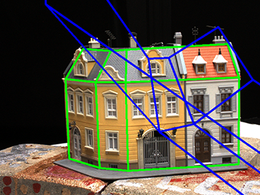
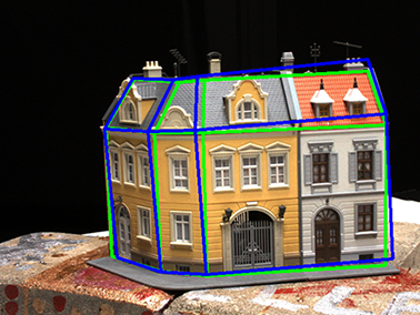
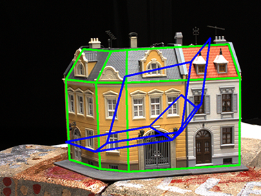
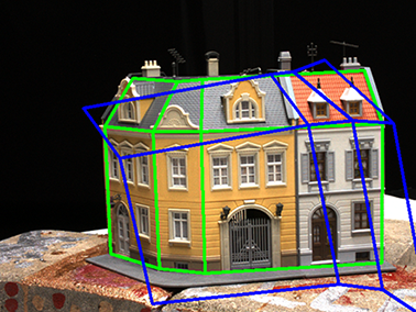
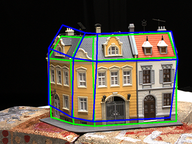
SIFT	SURF	ORB

Figure 6: Localization result of naïve method (top row), REST without whitening (middle row) and REST with whitening (bottom row). The green outline shows the ground truth outline of the building. The blue outline is the projection of the model given the estimated camera pose.

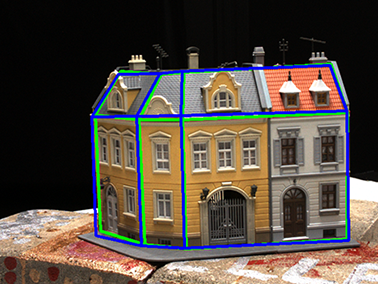
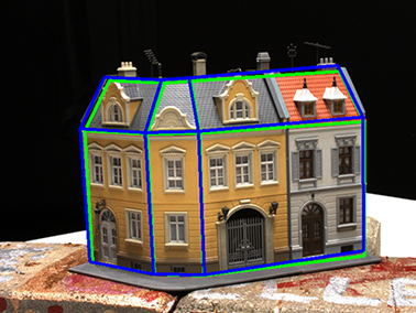
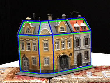
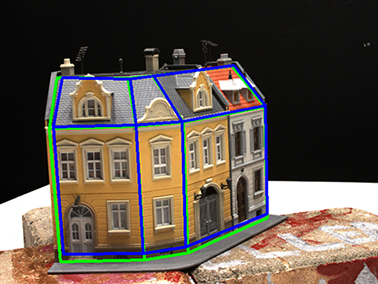
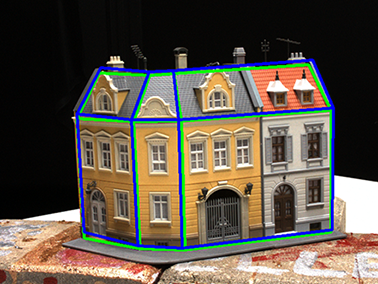
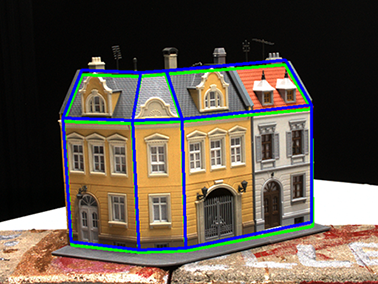
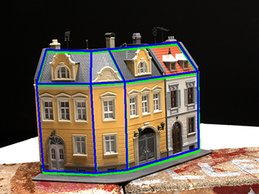
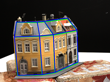
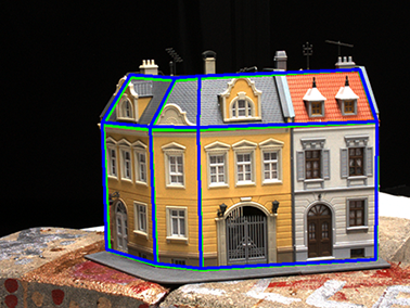
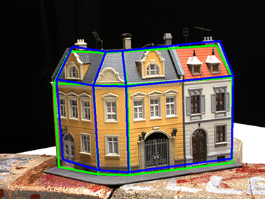
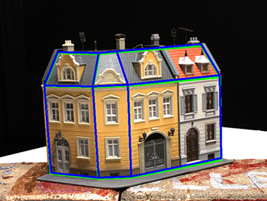
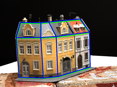
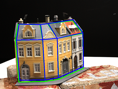
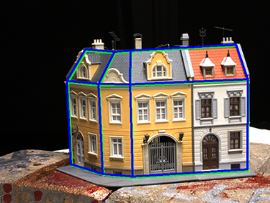
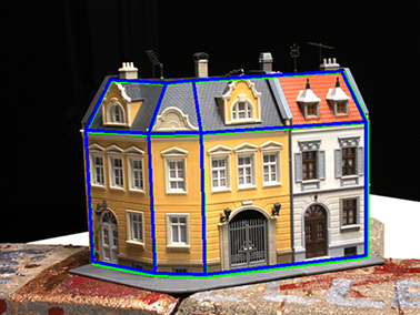
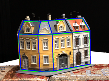
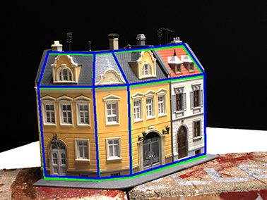
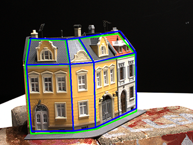
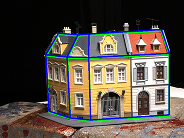
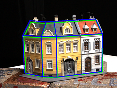
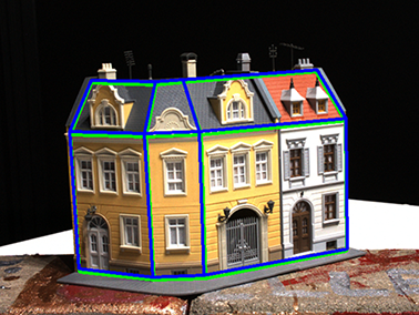
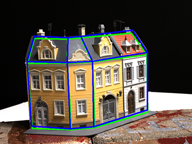
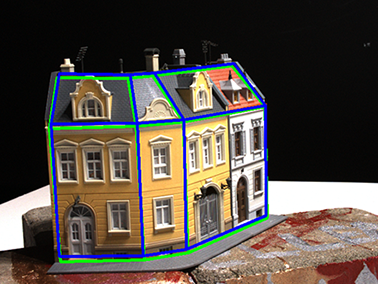
Figure 7: Localization Result of REST with whitening using SIFT under various conditions. Columns represent camera viewpoints and rows represent lighting conditions.

To evaluate what effect REST as well as whitening has on the feature matching and localization accuracy, we compare REST with whitening, REST without whitening, and naïve feature matching (directly matching a real feature with the synthetic feature database). We also evaluate how the chosen feature descriptor chosen affects the results. We compare three commonly used descriptors: SIFT [19], SURF [1], and ORB [26]. Since ORB is a binary feature descriptor, we split ORB features into float features by bits, i.e. 256-dimensional features.

We evaluate all methods on 60 images from the DTU dataset [7]. The images were selected to match the view a pedestrian usually looks at the building. Each image has a resolution of 640 $\times$ 480 pixel and we split them into 5 groups for cross validation. We train REST with 4 groups and evaluate matching accuracy with the left out group. The naïve method matches real features with the database using the same trained random forest as REST.

We judge a real feature as being correctly matched to its synthetic counterpart if the projection of the 3D location of the synthetic feature into the camera image, given the ground truth camera pose, is less than 3 pixel away from the detected real feature. This threshold is relatively small and is similar to  [16]. We show the results of the matching accuracy in Table 1.

REST improves the number of correctly matched features (MA) compared to the naïve approach for all feature descriptors. This indicates that REST successfully converts real features into synthetic features. Applying whitening further improves the matching results for all descriptors. ORB features performed worst in all tests, while SURF features were more robust to the gap and performed best during naïve matching. While this advantage persists for REST without whitening and with whitening, for REST with whitening SIFT features perform almost as well. The performance of REST without whitening SIFT features is worse than naïve matching. As discussed in Sec. 3.2, directly corresponding a real feature to a synthetic feature causes transformation a real feature into a synthetic feature in another feature clusters. As a result, REST decrease feature matching accuracy. We show the localization results using the different features in Fig. 6.

We evaluate the localization accuracy of the different methods. With the increasing ratio of correctly matched features we also observe improved localization accuracy. We show localization results of the naïve approach, REST without whitening, and REST with whitening for SIFT features in Fig. 6. The green outline shows the ground truth outline of the building, while the blue outline is the projection of the model given the estimated camera pose. REST with whitening is the only approach to recover an accurate camera pose. REST without whitening includes some outliers into which results in lower accuracy, while the naïve approach fails to correctly estimate the pose due to a low number of correct matches. The DTU dataset covers an area of approximately 1 m $\times$ 1 m. Overall, using SURF features leads to the best and most stable results. Interestingly, although the correct matching ratio for SIFT features increases for REST without whitening compared to the naïve approach, the localization accuracy decreases. However, it increases drastically for REST with whitening. This effect does not appear for SURF and ORB.

As stated in Sec. 1, lighting variation cause feature matching failure and decrease localization accuracy [21]. Whereas, REST with whitening for SIFT can estimate the correct camera poses from real images under different camera positions and lighting conditions shown in Fig. 7. Each columns represent a camera viewpoint and each rows represent a lighting condition. Thus, our approach is robust to variation of camera viewpoints and lighting conditions.

5.2 Comparison with PoseNet

Table 2: Result of comparison with PoseNet. From left column, position error (PE), orientation error (OE), and localization time are indicated.

Net	Image		$\mathrm{PE}$	$\mathrm{OE}$	$\mathrm{Time}$
PoseNet	real	mean	$37.21\ \mathrm{cm}$	$25.33^{\circ}$	$\bm{14.05}\ \mathrm{ms}$
		median	$37.17\ \mathrm{cm}$	$25.69^{\circ}$	$\bm{13.17}\ \mathrm{ms}$
	syn.	mean	$3.87\ \mathrm{cm}$	$10.87^{\circ}$	$13.30\ \mathrm{ms}$
		median	$3.64\ \mathrm{cm}$	$11.00^{\circ}$	$13.05\ \mathrm{ms}$
REST	real	mean	$\bm{5.55}\ \mathrm{cm}$	$\bm{6.38}^{\circ}$	$340.50\ \mathrm{ms}$
SIFT w/ whitening		median	$\bm{1.89}\ \mathrm{cm}$	$\bm{1.64}^{\circ}$	$339.90\ \mathrm{ms}$

We also compare our method with a CNN-based localization method on synthetic images. We trained PoseNet [11] on the same dataset that was used to generate the database. To verify the training quality we evaluate the PoseNet localization results on synthetic images that were not part of the training. PoseNet achieves high positional accuracy, while the rotation has an error of up to 11^∘. However, when a real image is used instead, the positional and rotational accuracy degrades significantly. Overall, PoseNet performs worse than our approach. We show the results of PoseNet estimation in Table 2. This indicates that the gap between simulated and real images also has a significant effect on CNN-based methods and correction with GAN-based methods is necessary. However, as training a GAN requires a large number of images it is not viable to simulate variable lighting conditions.

However, localization time of our method is slow than PoseNet. This is because feature description and feature matching with a random forest are time-consuming. Since camera localization is only required at the first frame of tracking and when tracking was lost. Thus, Our localization with the update rate of 350 ms is enough to camera localization. note that, our system run on CPU, which still have room for further optimization of localization time.

6 Conclusion and Future Work

In this paper we presented a new approach for robust camera localization in varying lighting conditions. We use a feature database generated from synthetic images that simulate the appearance of the scene under different lighting conditions. Sicne the synthetic data does not perfectly match the scene appearance, it is necessary to overcome the appearance gap between simulation and reality.

We introduce REST, an autoencoder-like network that converts feature descriptors extracted from real images into descriptors which similar to the descriptors that would be extracted from synthetic images generated under the same conditions. We also use whitening process to improve the matching ratio between real and synthetic features. Our pipeline successfully improves the matching ratio between real images and the feature database. Our experimental results show that the appearance gap clearly affects CNN-based localization methods. Therefore, methods trained only on synthetic images fail to correctly localize the camera.

Since REST converts a real feature into a synthetic feature which might not always matched with feature database. For the future work, we plan to improve our system so that it can convert a real feature to a feature that is easily matched to feature database. This improves not only the accuracy of camera localization but also localization time because simpler and faster feature matching can be achieved without random forests.

References

- [1] H. Bay, A. Ess, T. Tuytelaars, and L. V. Gool. SURF: Speeded Up Robust Features. In Proceedings of European Conference on Computer Vision (ECCV), pp. 404–417, 2006.
- [2] F. Calakli and G. Taubin. SSD: Smooth Signed Distance Surface Reconstruction. Computer Graphics Forum, 30(7):1993–2002, 2011.
- [3] J. Engel, T. Schöps, and D. Cremers. LSD-SLAM: Large-scale Direct Monocular SLAM. In Proceedigns of European Conference on Computer Vision (ECCV), pp. 834–849, 2014.
- [4] J. Engel, J. Sturm, and D. Cremers. Semi-dense Visual Odometry for a Monocular Camera. In Proceedings of International Conference on Computer Vision (ICCV), pp. 1449–1456, 2013.
- [5] M. A. Fischler and R. C. Bolles. Random Sample Consensus: A Paradigm for Model Fitting with Applications to Image Analysis and Automated Cartography. Communications, 24(6):381–395, 1981.
- [6] G. E. Hinton and R. R. Salakhutdinov. Reducing the Dimensionality of Data with Neural Networks. Science, 313:504–507, 2006.
- [7] R. Jensen, A. Dahl, G. Vogiatzis, E. Tola, and H. Aanæs. Large Scale Multi-view Stereopsis Evaluation. In Proceedings of Conference on Computer Vision and Pattern Recognition (CVPR), pp. 406–413, 2014.
- [8] M. Kazhdan, M. Bolitho, and H. Hoppe. Poisson Surface Reconstruction. In Proceedings of Eurographics Symposium on Geometry Processing (SGP), pp. 61–70, 2006.
- [9] M. Kazhdan and H. Hoppe. Screened Poisson Surface Reconstruction. Transactions on Graphics (TOG), 32(3), 2013.
- [10] A. Kendall and R. Cipolla. Modeling Uncertainty in Deep Learning for Camera Relocalization. In Proceedings of International Conference on Robotics and Automation (ICRA), pp. 4762–4769, 2016.
- [11] A. Kendall, M. Grimes, and R. Cipolla. PoseNet: A Convolutional Network for Real-time 6-DOF Camera Relocalization. In Proceedings of International Conference on Computer Vision (ICCV), pp. 2938–2946, 2015.
- [12] C. Kerl, J. Sturm, and D. Cremers. Dense Visual SLAM for RGB-D Cameras. In Proceedings of Intelligent Robots and Systems, pp. 2100–2106, 2013.
- [13] A. Krizhevsky. Learning multiple layers of features from tiny images, 2009.
- [14] A. Krizhevsky, I. Sutskever, and G. E. Hinton. ImageNet: Classification with Deep Convolutional Neural Networks. In Proceedings of Annual Conference on Neural Information Processing Systems (NIPS), pp. 1097–1105, 2012.
- [15] A. Kull, E. Brachmann, F. Michel, M. Y. Yang, S. Gumhold, and C. Rother. Learning Analysis-by-Synthesis for 6D Pose Estimation in RGB-D Images. In Proceedings of International Conference on Computer Vision (ICCV), pp. 954–962, 2015.
- [16] D. Kurz, P. Meier, A. Plopski, and G. Klinker. Absolute Spatial Context-aware Visual Descriptors for Outdoor Handheld Camera Localization. In Proceedings of International Conference on Computer Vision Theory and Applications (VISAPP), pp. 36–42, 2014.
- [17] D. Kurz, P. G. Meier, A. Plopski, and G. Klinker. An Outdoor Ground Truth Evaluation Dataset for Sensor-aided Visual Handheld Camera Localization. In Proceedings of International Symposium on Mixed and Augmented Reality (ISMAR), pp. 263–264, 2013.
- [18] D. Kurz, T. Olszamowski, and S. Benhimane. Representative Feature Descriptor Sets for Robust Handheld Camera Localization. In Proceedings of International Symposium on Mixed and Augmented Reality (ISMAR), pp. 65–70, 2012.
- [19] D. Lowe. Distinctive Image Features from Scale-invariant Keypoints. International Journal of Computer Vision (IJCV), 60(2):91–110, 2004.
- [20] Y. Ma and Košecká, J. and Soatto, S. and Sastry, S. An invitation to 3-d vision: From images to models. Springer Science & Business Media.
- [21] T. Mashita, A. Plopski, A. Kudo, T. Höllerer, K. Kiyokawa, and H. Takemura. Simulation based Camera Localization under a Variable Lighting Environment. In Proceedings of International Conference on Advanced Technology & Science (ICAT), 2016.
- [22] R. Mur-Artal, J. M. M. Montiel, and J. D. Tardós. ORB-SLAM: A Versatile and Accurate Monocular SLAM System. IEEE Transactions on Robotics (T-Ro), 31(5):1147–1163, 2015.
- [23] R. A. Newcombe, S. Izadi, O. Hilliges, D. Molyneaux, D. Kim, A. J. Davison, P. Kohi, J. Shotton, S. Hodges, and A. Fitzgibbon. KinectFusion: Real-time Dense Surface Mapping and Tracking. In Proceedings of International Symposium on Mixed and Augmented Reality (ISMAR), pp. 127–136, 2011.
- [24] R. A. Newcombe, S. J. Lovegrove, and A. J. Davison. DTAM: Dense Tracking and Mapping in Real-time. In Proceedings of International Conference on Computer Vision (ICCV), pp. 2320–2327, 2011.
- [25] T. Rattenbury, N. Good, and M. Naaman. Towards Automatic Extraction of Event and Place Semantics from Flickr Tags. In Proceedings of Annual International Conference on Research and Development in Information Retrieval, pp. 103–110, 2007.
- [26] E. Rublee, V. Raubaud, K. Konolige, and K. Bradsky. ORB: An Efficient Alternative to SIFT or SURF. In Proceedings of International Conference on Computer Vision (ICCV), pp. 264–2571, 2011.
- [27] Y. Shinozuka, F. d. Sorbler, and H. Saito. Specular 3D Object Tracking by View Generative Learning. In Proceedings of Irish Machine Vision and Image Processing (IMVIP), pp. 9–14, 2014.
- [28] A. Shrivastava, T. Pfister, O. Tuzel, J. Susskind, W. Wang, and R. Webb. Learning from Simulated and Unsupervised Images through Adversarial Training. In Proceedings of Conference on Computer Vision and Pattern Recognition (CVPR), pp. 2242–2251, 2017.
- [29] G. Simon. Tracking-by-Synthesis Using Point Features and Pyramidal Blurring. In Proceedings of International Symposium and Augmented Reality (ISMAR), pp. 85–92, 2011.
- [30] H. Su, C. R. Qi, Y. Li, and L. J. Guibas. Render for CNN: Viewpoint Estimation in Images Using CNNs Trained with Rendered 3D Model Views. In Proceedings International Conference on Computer Vision (ICCV), pp. 2686–2694, 2015.
- [31] C. Szegedy, W. Liu, Y. Jia, P. Sermanet, S. Reed, D. Anguelov, D. Erhan, V. Vanhoucke, and A. Rabinovich. Going Deeper with Convolutions. In Proceedings of Conference on Computer Vision and Pattern Recognition (CVPR), 2015.
- [32] K. Tateno, R. Tombari, I. Laina, and N. Navab. CNN-SLAM: Real-time Dense Monocular SLAM with Lerned Depth Prediction. In Proceedings of Conference on Computer Vision and Pattern Recognition (CVPR), pp. 6565–6574, 2017.
- [33] P. Vincent, H. Larochelle, I. Lojoie, Y. Bengio, and P. A. Manzagol. Stacked Denoising Autoencoders: Learning Useful Representations in a Deep Neural Network with a Local Denoising Criterion. Journal of Machine Learning Research (JMLR), 11:3371–3408, 2010.
- [34] F. Walch, C. Hazirbas, L. Leal-Taixé, T. Sattler, S. Hilsenbeck, and D. Cremers. Image-based Localization using LSTMs for Structured Feature Correlation. In Proceedings of International Conference on Computer Vision (ICCV), 2017.
- [35] K. M. Yi, E. Trulls, V. Lepetit, and P. Fua. LIFT: Learned Invariant Feature Transform. In Proceedings of European Conference on Computer Vision (ECCV), pp. 467–483, 2016.