Convergent kernel-based methods for parabolic equations

Abstract

We prove that the functions constructed by the kernel-based regressions with Wendland kernels under $\ell_{1}$-norm constraints converge to unique viscosity solutions of the corresponding fully nonlinear parabolic equations. A key ingredient in our proof is the max-min representations of the nonlinearities of the equations.

Key words: Nonlinear parabolic equations, kernel-based approximation, viscosity solutions, radial basis functions, Hamilton-Jacobi-Bellman equations.

AMS MSC 2010: 65M70, 35K55.

1 Introduction

In this paper, we are concerned with the rigorous convergence of the kernel-based methods for the terminal value problems of the parabolic partial differential equations:

(1.1) $$\left\{\begin{split}&-\partial_{t}v+F(t,x,v(t,x),Dv(t,x),D^{2}v(t,x))=0,\quad(t,x)\in[0,T)\times\mathbb{R}^{d},\\ &v(T,x)=f(x),\quad x\in\mathbb{R}^{d},\end{split}\right.$$

where $F:[0,T]\times\mathbb{R}^{d}\times\mathbb{R}\times\mathbb{R}^{d}\times\mathbb{S}^{d}\to\mathbb{R}$, and $\mathbb{S}^{d}$ stands for the totality of symmetric $d\times d$ real matrices. Here we have denoted by $\partial_{t}$ the partial differential with respect to the time variable $t$, by $D$ and $D^{2}$ the gradient and Hessian with respect to the spatial variable $x$, respectively. Under suitable conditions including the degenerate ellipticity on $F$, the terminal value problem (1.1) has a unique viscosity solution $v$. In the case where (1.1) is of Hamilton-Jacobi-Bellman type, it is well known that we can obtain an optimal policy for a stochastic control problem by solving (1.1). Popular numerical methods for (1.1) include the finite difference methods (see, e.g., Kushner and Dupuis [11] and Bonnans and Zidani [2]), the finite-element like methods (see, e.g., Camilli and Falcone [3] and Debrabant and Jakobsen [5]), and the probabilistic methods (see, e.g., Pagès et al. [14], Fahim et al. [6], Guo et.al [7] and Nakano [12]).

The methods analyzed in the present paper consist of the kernel-based regressions applied backward recursively in time. Given a points set $\Gamma=\{x_{1},\ldots,x_{N}\}\subset\mathbb{R}^{d}$ such that $x_{j}$’s are pairwise distinct, and a positive definite function $\Phi:\mathbb{R}^{d}\to\mathbb{R}$, we solve a least-square problem

(1.2) $$\min\sum_{j=1}^{N}\left|u(x_{j})-\sum_{\ell=1}^{M}\gamma_{\ell}\Phi(x_{j}-\xi_{\ell})-c\right|^{2},$$

$$\text{s.t.}\quad\sum_{\ell=1}^{M}|\gamma_{\ell}|+|c|\leq\beta,\;\;\gamma_{\ell},c\in\mathbb{R},\;\;\xi_{\ell}\in\mathbb{R}^{d},\;\;\ell=1,\ldots,M,$$

where $\beta$ is a given positive constant and $M\in\mathbb{N}$. If $\beta=+\infty$ and $M=N$, the minimizer is

$$\sum_{j=1}^{N}(A^{-1}u|_{\Gamma})_{j}\Phi(x-x_{j}),\quad x\in\mathbb{R}^{d},$$

the interpolation function of $u$ on $\Gamma$. Here, $A=\{\Phi(x_{j}-x_{\ell})\}_{j,\ell=1,\ldots,N}$, $u|_{\Gamma}$ is the column vector composed of $u(x_{j})$, $j=1,\ldots,N$, and $(z)_{j}$ denotes the $j$-th component of $z\in\mathbb{R}^{N}$. Thus, with time grid $\{t_{0},\ldots,t_{n}\}$ such that $0=t_{0}<\cdots<t_{n}=T$, the function $v^{h}(t_{n},\cdot)$ defined by

(1.3) $$v^{h}(t_{n},x)=\sum_{\ell=1}^{M}\gamma_{n,\ell}\Phi(x-\xi_{n,\ell})+c_{n},\quad x\in\mathbb{R}^{d},$$

approximates $f$, where $(\gamma_{n,1},\ldots,\gamma_{n,M},\xi_{n,1},\ldots,\xi_{n,M},c_{n})$ is an $\varepsilon$-optimal solution of (1.2) for $u=f$. Then for any $k=0,1,\ldots,n-1$, the function $v^{h}(t_{k},\cdot)$ recursively defined by

(1.4) $$v^{h}(t_{k},x)=v^{h}(t_{k+1},x)-(t_{k+1}-t_{k})\left(\sum_{\ell=1}^{M}\gamma_{k+1,\ell}\Phi(x-\xi_{k+1,\ell})+c_{k+1}\right)$$

can be a candidate of approximate solution to (1.1). Here, $(\gamma_{k,1},\ldots,\gamma_{k,M},\xi_{k,1},\ldots,\xi_{k,M},c_{k})$ is an $\varepsilon$-optimal solution of (1.2) for $u=F(t_{k},\cdot,v^{h}(t_{k},\cdot),Dv^{h}(t_{k},\cdot),D^{2}v^{h}(t_{k},\cdot))$.

In the unconstrained case with $M=N$, the method above is simply described as follows:

(1.5) $$v^{h}(t_{k+1},x) =\sum_{j=1}^{N}(A^{-1}v^{h}_{k+1})_{j}\Phi(x-x^{(j)}),\quad x\in\mathbb{R}^{d},$$

$$v^{h}_{k} =v^{h}_{k+1}-(t_{k+1}-t_{k})F_{k+1}(v_{k+1}^{h}),\quad k=0,\ldots,n-1,$$

$$v^{h}_{n} =f|_{\Gamma},$$

where $F_{k+1}(v_{k+1}^{h})=(F_{k+1,1}(v_{k+1}^{h}),\ldots,F_{k+1,N}(v_{k+1}^{h}))\in\mathbb{R}^{N}$ with

$$F_{k+1,j}=F(t_{k+1},x^{(j)},v^{h}(t_{k+1},x^{(j)}),Dv^{h}(t_{k+1},x^{(j)}),D^{2}v^{h}(t_{k+1},x^{(j)})).$$

This is the kernel-based (or meshfree) collocation method proposed by Kansa [9]. Although the method gains popularity since it allows for simpler implementation in multi-dimensional cases, rigorous convergence issue remains unresolved completely. Hon et.al [8] obtains an error bound for a special heat equation in one dimension. Nakano [13] shows the convergence for fully nonlinear parabolic equations of the form (1.1) under some normative assumptions on the kernel-based interpolations.

In the present paper, we show that the function $v^{h}$ defined by (1.3) and (1.4) converges to $v$ in the cases where $\Phi$ is a Wendland kernel. A key ingredient in our proof is the max-min representations of the nonlinearities of the parabolic equations obtained in [13]. This result enables us to drop the monotonicity condition in the viscosity solution method by Barles and Souganidis [1] in handling smooth approximate functions. In the convergence analysis, the stability of the approximate solution is essential, and so we impose the $\ell_{1}$-type constraint in the regression. Thus the interpolation method defined by (1.5) is difficult to handle theoretically and is outside scope of the convergence issue in this paper. Here we consider the interpolation method a practical alternative to the regression one with constraint.

This paper is organized as follows. The next section presents a brief summary of interpolation theory with reproducing kernels. We explain the kernel-based methods in details in Section 3. The main convergence theorem is described and proved in Section 4. In Section 5 we perform several numerical experiments.

2 Multivariate interpolation with reproducing kernels

In this section, we recall the basis of the multivariate interpolation theory with reproducing kernels. We refer to Wendland [15] for a complete account. In what follows, we denote $|a|=(\sum_{i=1}^{m}\sum_{j=1}^{k}(a_{ij})^{2})^{1/2}$ for $a=(a_{ij})\in\mathbb{R}^{m\times k}$. Let $\mathcal{O}$ be an open hypercube in $\mathbb{R}^{d}$, and let $\Phi:\mathbb{\mathbb{R}}^{d}\to\mathbb{R}$ be a radial and positive definite function, i.e., $\Phi(\cdot)=\phi(|\cdot|)$ for some $\phi:[0,\infty)\to\mathbb{R}$ and for every $\ell\in\mathbb{N}$, for all pairwise distinct $y_{1},\ldots,y_{\ell}\in\mathbb{R}^{d}$ and for all $\alpha=(\alpha_{i})\in\mathbb{R}^{\ell}\setminus\{0\}$, we have

$$\sum_{i,j=1}^{\ell}\alpha_{i}\alpha_{j}\Phi(y_{i}-y_{j})>0.$$

Then, by Theorems 10.10 and 10.11 in [15], there exists a unique Hilbert space $\mathcal{N}_{\Phi}(\mathcal{O})$ with norm $\|\cdot\|_{\mathcal{N}_{\Phi}(\mathcal{O})}$, called the native space, of real-valued functions on $\mathcal{O}$ such that $\Phi$ is a reproducing kernel for $\mathcal{N}_{\Phi}(\mathcal{O})$.

Let $\Gamma=\{x_{1},\cdots,x_{N}\}$ be a finite subset of $\mathcal{O}$ such that $x_{j}$’s are pairwise distinct and put $A=\{\Phi(x_{i}-x_{j})\}_{1\leq i,j\leq N}$. Then $A$ is invertible and thus for any $g:\mathcal{O}\to\mathbb{R}$ the function

$$I(g)(x)=\sum_{j=1}^{N}(A^{-1}g|_{\Gamma})_{j}\Phi(x-x_{j}),\quad x\in\mathcal{O},$$

interpolates $g$ on $\Gamma$.

Suppose that $\Phi$ is a $C^{2\kappa}$-function on $\mathcal{O}$. Then there exists a positive constant $C_{\Phi,\mathcal{O}}$ depending only on $\Phi$ and $\mathcal{O}$ such that for any $g\in\mathcal{N}_{\Phi}(\mathcal{O})$ and multi-index $\alpha=(\alpha_{1},\ldots,\alpha_{d})$ with $|\alpha|_{1}:=\alpha_{1}+\cdots+\alpha_{d}\leq\kappa$ we have

(2.1) $$|D^{\alpha}g(x)-D^{\alpha}I(g)(x)|\leq C_{\Phi,\mathcal{O}}(\Delta x)^{\kappa-|\alpha|_{1}}\|g\|_{\mathcal{N}_{\Phi}(\mathcal{O})},\quad x\in\mathcal{O},$$

provided that the Hausdorff distance $\Delta x$ between $\Gamma$ and $\mathcal{O}$, given by

$$\Delta x=\sup_{x\in\mathcal{O}}\min_{j=1,\ldots,N}|x-x_{j}|,$$

is sufficiently small. Here, the differential operator $D^{\alpha}$ is defined as usual by

$$D^{\alpha}g(x_{1},\ldots,x_{d})=\frac{\partial^{|\alpha|_{1}}}{\partial x_{1}^{\alpha_{1}}\cdots\partial x_{d}^{\alpha_{d}}}g(x_{1},\ldots,x_{d}),\quad\alpha=(\alpha_{1},\ldots,\alpha_{d}).$$

See Theorem 11.13 in [15].

The so-called Wendland kernel is a typical example of radial and positive definite functions on $\mathbb{R}^{d}$, which is defined as follows: for a given $\tau\in\mathbb{N}\cup\{0\}$, set the function $\Phi_{d,\tau}$ satisfying $\Phi_{d,\tau}(x)=\phi_{d,\tau}(|x|)$, $x\in\mathbb{R}^{d}$, where

$$\phi_{d,\tau}(r)=\int_{r}^{\infty}r_{\tau}\int_{r_{\tau}}^{\infty}r_{\tau-1}\int_{r_{\tau-1}}^{\infty}\cdots\>r_{2}\int_{r_{2}}^{\infty}r_{1}\max\{1-r_{1},0\}^{\nu}dr_{1}dr_{2}\cdots dr_{\tau},\quad r\geq 0$$

for $\tau\geq 1$ and $\phi_{d,\tau}(|x|)=\max\{1-r,0\}^{\nu}$ for $\tau=0$ with $\nu=\max\{m\in\mathbb{Z}:m\leq\tau+d/2+1\}$. Then, it follows from Theorems 9.12 and 9.13 in [15] that the function $\phi_{d,\tau}$ is represented as

$$\phi_{d,\tau}(r)=\begin{cases}p_{d,\tau}(r),&0\leq r\leq 1,\\ 0,&r>1,\end{cases}$$

where $p_{d,\tau}$ is a univariate polynomial with degree $\nu+2\tau$ having representation

(2.2) $$p_{d,\tau}(r)=\sum_{j=0}^{\nu+2\tau}d_{j,\tau}^{(\nu)}r^{j}.$$

The coefficients in (2.2) are given by

$$d_{j,0}^{(\nu)} =(-1)^{j}\frac{\nu!}{j!(\nu-j)!},\quad 0\leq j\leq\ell,$$

$$d_{0,s+1}^{(\nu)} =\sum_{j=0}^{\nu+2s}\frac{d_{j,s}^{(\nu)}}{j+2},\quad d_{1,s+1}^{(\nu)}=0,\quad s\geq 0,$$

$$d_{j,s+1}^{(\nu)} =-\frac{d_{j-2,s}^{(\nu)}}{j},\quad s\geq 0,\quad 2\leq j\leq\nu+2s+2,$$

in a recursive way for $0\leq s\leq\tau-1$. Further, it is known that

$$\phi_{d,\tau}(r)\doteq\begin{cases}\displaystyle\int_{r}^{1}s(1-s)^{\nu}(s^{2}-r^{2})^{\tau-1}ds,&0\leq r\leq 1,\\[10.00002pt] 0,&r>1,\end{cases}$$

where $\doteq$ denotes equality up to a positive constant factor (see Chernih et.al [4]). For example,

$$\phi_{1,2}(r) \doteq\max\{1-r,0\}^{5}(8r^{2}+5r+1),$$

$$\phi_{1,3}(r) \doteq\max\{1-r,0\}^{7}(21r^{3}+19r^{2}+7r+1),$$

$$\phi_{1,4}(r) \doteq\max\{1-r,0\}^{9}(384r^{4}+453r^{3}+237r^{2}+63r+7),$$

$$\phi_{2,4}(r) \doteq\max\{1-r,0\}^{10}(429r^{4}+450r^{3}+210r^{2}+50r+5),$$

$$\phi_{2,5}(r) \doteq\max\{1-r,0\}^{12}(2048r^{5}+2697r^{4}+1644r^{3}+566r^{2}+108r+9).$$

It is known that the function $\Phi_{d,\tau}$ is of $C^{2\tau}$-class on $\mathbb{R}^{d}$, and the native space $\mathcal{N}_{\Phi_{d,\tau}}(\mathcal{O})$ coincides with the Sobolev space $H^{\tau+(d+1)/2}(\mathcal{O})$ on $\mathcal{O}$ of order $\tau+(d+1)/2$ based on $L^{2}$-norm.

3 Kernel-based methods

In what follows, the function $\Phi$ is assumed to be the Wendland kernel $\Phi_{d,\tau}$ divided by some positive constant with fixed $\tau\geq 2$. Let $h>0$ be a parameter that describes approximate solutions, $\Gamma=\{x_{1},\ldots,x_{N}\}\subset(-R,R)^{d}$ with $R>0$, and $\{t_{0},\ldots,t_{n}\}$ the set of the uniform time grid points such that $t_{0}=0$ and $t_{n}=T$. Let $\beta_{M}$ be an increasing and positive sequence such that $\beta_{M}\to\infty$ as $M\to\infty$. We consider the function

$$G_{M}(x;\theta):=\sum_{\ell=1}^{M}\gamma_{j}\Phi(x-\xi_{j})+c,\quad x\in\mathbb{R}^{d},\;\;\theta\in\mathcal{R}_{M},$$

where

$$\mathcal{R}_{M}=\left\{\theta=(\gamma_{1},\ldots,\gamma_{M},\xi_{1},\ldots,\xi_{M},c):\begin{aligned} &\sum_{\ell=1}^{M}|\gamma_{\ell}|+|c|\leq\beta_{M},\\ &\gamma_{1},\ldots,\gamma_{M},c\in\mathbb{R},\;\;\xi_{1},\ldots,\xi_{M}\in\mathbb{R}^{d}\end{aligned}\right\}.$$

Then, for a given $u:\mathbb{R}^{d}\to\mathbb{R}$, $\varepsilon>0$ and $M\in\mathbb{N}$, there exists $\theta_{u}^{(\varepsilon,M)}\in\mathcal{R}_{M}$ such that

(3.1) $$\sum_{j=1}^{N}|u(x_{j})-G_{M}(x_{j};\theta_{u}^{(\varepsilon,M)})|^{2}\leq\inf_{\theta\in\mathcal{R}_{M}}\sum_{j=1}^{N}|u(x_{j})-G_{M}(x_{j};\theta)|^{2}+\varepsilon^{2}.$$

As described in Section 1, we define the function $v^{h}(t_{n},\cdot)$ by

(3.2) $$v^{h}(t_{n},x)=G_{M}(x_{j};\theta_{n}^{(h,M)}),\quad x\in\mathbb{R}^{d},$$

where $\theta_{n}^{(h,M)}=\theta_{f}^{(\varepsilon,M)}$ for $u=f$ and $\varepsilon=h$. For $k=0,\ldots,n-1$, we define the function $v^{h}(t_{k},\cdot)$ recursively by

(3.3) $$v^{h}(t_{k},x)=v^{h}(t_{k+1},x)-(t_{k+1}-t_{k})G_{M}(x_{j};\theta_{k+1}^{(h,M)}),\quad x\in\mathbb{R}^{d}.$$

Here, $\theta_{k+1}^{(h,M)}=\theta_{u}^{(\varepsilon,M)}$ in (3.1) for $u=F(t_{k+1},\cdot;v(t_{k+1},\cdot))$ and $\varepsilon=h$ where for any $C^{2}$-function $\varphi$ on $\mathbb{R}^{d}$,

$$F(t,x;\varphi)=F(t,x,\varphi(x),D\varphi(x),D^{2}\varphi(x)),\quad x\in\mathbb{R}^{d}.$$

The unconstrained case with $M=N$ allows much simpler implementation if the computation of the matrix inverse $A^{-1}$ has no difficulty. As described in Section 1, we define the function $\bar{v}^{h}$ by

(3.4) $$\bar{v}^{h}(t_{k},x)=\sum_{j=1}^{N}(A^{-1}v^{h}_{k})_{j}\Phi(x-x^{(j)}),\quad x\in\mathbb{R}^{d},$$

with

(3.5) $$\left\{\begin{aligned} &v_{k}^{h}=v_{k+1}^{h}-(t_{k+1}-t_{k})F_{k+1}(v_{k+1}^{h}),\quad k=0,\ldots,n-1,\\ &v_{n}^{h}=f|_{\Gamma},\end{aligned}\right.$$

where $F_{k,j}(v_{k}^{h})=F(t_{k},x^{(j)};v^{h}(t_{k},\cdot))$ and $F_{k}(v_{k}^{h})=(F_{k,1}(v_{k}^{h}),\ldots,F_{k,N}(v_{k}^{h}))^{\mathsf{T}}$.

Remark 3.1.

The linearity of the interpolant yields, for $x\in\mathbb{R}^{d}$,

$$\bar{v}^{h}(t_{k},x)=\bar{v}^{h}(t_{k+1},x)-(t_{k+1}-t_{k})I(F_{k+1}(v_{k+1}^{h}))(x),$$

where by abuse of notation we denote $I(\xi)(x)=\sum_{j=1}^{N}(A^{-1}\xi)_{j}\Phi(x-x^{(j)})$ for $\xi\in\mathbb{R}^{N}$.

Let us describe our interpolation methods in a matrix form. To this end, we assume here that the nonlinearity $F$ can be written as

$$F(t,x;\varphi)=\sup_{\pi\in K}H(t,x,\varphi(x),b(x,\pi)^{\mathsf{T}}D\varphi(x),\mathrm{tr}(a(x,\pi)D^{2}\varphi(x))),$$

where $K$ is a set, $b:\mathbb{R}^{d}\times K\to\mathbb{R}^{d}$, $a:\mathbb{R}^{d}\times K\to\mathbb{S}^{d}$, and $H:[0,T]\times\mathbb{R}^{d}\times\mathbb{R}\times\mathbb{R}\times\mathbb{R}\to\mathbb{R}$. It should be noted that the nonlinearities corresponding to Hamilton-Jacobi-Bellman equations are represented in this form. Then, consider the function $\phi_{d,\tau}^{(1)}(r):=\phi_{d,\tau}^{\prime}(r)/r$, $r\geq 0$. By definition of $\phi_{d,\tau}$, the function $\phi^{(1)}_{d,\tau}$ is continuous on $[0,\infty)$ and supported in $[0,1]$. With this function, we have

$$\frac{\partial}{\partial_{x_{m}}}\Phi(x)=\phi^{(1)}(|x|)x_{m},\quad x=(x_{1},\ldots,x_{d})\in\mathbb{R}^{d}.$$

Thus,

$$B_{\ell}(\pi):=\left(b_{\ell}(x^{(i)},\pi)\frac{\partial\Phi}{\partial_{x_{\ell}}}(x^{(i)}-x^{(j)})\right)_{1\leq i,j\leq N}=Q_{\ell}(\pi)(G_{\ell}A_{1}-A_{1}G_{\ell}),$$

where $Q_{\ell}(\pi)=\mathrm{diag}(b_{\ell}(x^{(1)},\pi),\ldots,b_{\ell}(x^{(N)},\pi))$, $A_{1}=\{\phi_{d,\tau}^{(1)}(|x^{(i)}-x^{(j)}|)\}_{1\leq i,j\leq N}$ and $G_{\ell}=\mathrm{diag}(x^{(1)}_{\ell},\ldots,x^{(N)}_{\ell})$. Hence,

$$\mathbb{R}^{N}\ni(b_{\ell}(x^{(i)},\pi)(\partial/\partial_{x_{\ell}})I(\xi)(x^{(i)}))_{1\leq i\leq N}=B_{\ell}(\pi)A^{-1}\xi.$$

Similarly,

$$\frac{\partial^{2}}{\partial x_{m}x_{\ell}}\Phi(x)=\begin{cases}\phi_{d,\tau}^{(1)}(|x|)+\phi^{(2)}_{d,\tau}(|x|)x_{m}^{2},&(\ell=m),\\ \phi_{d,\tau}^{(2)}(|x|)x_{m}x_{\ell},&(\ell\neq m),\end{cases}$$

where

$$\phi_{d,\tau}^{(2)}(r)=\frac{1}{r}\frac{d\phi_{d,\tau}^{(1)}}{dr}(r),\quad r\geq 0.$$

Notice that $\phi_{d,\tau}^{(2)}$ is also continuous on $[0,\infty)$ and supported in $[0,1]$. Thus,

$$B_{m\ell}(\pi):=\left\{(a_{m\ell}(x^{(i)},\pi)\frac{\partial^{2}\Phi}{\partial_{x_{m}x_{\ell}}}(x^{(i)}-x^{(j)})\right\}_{1\leq i,j\leq N}$$

is given by

$$B_{mm}(\pi)=Q_{mm}(\pi)(A_{1}+G_{m}^{2}A_{2}-2G_{m}A_{2}G_{m}+A_{2}G_{m}^{2})$$

and for $m\neq\ell$,

$$B_{m\ell}=Q_{m\ell}(\pi)(G_{m}G_{\ell}A_{2}-G_{m}A_{2}G_{\ell}-G_{\ell}A_{2}G_{m}+A_{2}G_{m}G_{\ell})$$

with $A_{2}=\{\phi_{d,\tau}^{(2)}(|x^{(i)}-x^{(j)}|)\}_{1\leq i,j\leq N}$ and $Q_{m\ell}(\pi)=\mathrm{diag}(a_{m\ell}(x^{(1)},\pi),\ldots,a_{m\ell}(x^{(N)},\pi))$. Consequently, we obtain

$$F_{k,j}(v_{k}^{h})=\sup_{\pi\in K}H\left(t_{k},x^{(j)},v^{h}_{k,j},\left(\sum_{m=1}^{d}B_{m}(\pi)A^{-1}v_{k}^{h}\right)_{j},\left(\sum_{m,\ell=1}^{d}B_{m\ell}(\pi)A^{-1}v_{k}^{h}\right)_{j}\right).$$

Thus, if the computation of $A^{-1}$ and the matrix product require $S_{1}(d,N)$ time and $S_{2}(N)$ time, respectively, and if the both are greater than $O(N^{2})$, then the total time for our algorithm is $O(S_{1}(d,N)+nd^{2}S_{2}(N))$.

4 Convergence

We study a convergence of the approximation method described in Section 3 under the conditions where (1.1) admits a unique viscosity solution. To this end, first we recall the notion of the viscosity solution and describe our standing assumptions for (1.1).

An $\mathbb{R}$-valued, upper-semicontinuous function $u$ on $[0,T]\times\mathbb{R}^{d}$ is said to be a viscosity subsolution of (1.1) if the following two conditions hold:

• for every $(t,x)\in[0,T)\times\mathbb{R}^{d}$ and every smooth function $\varphi$ such that $0=(u-\varphi)(t,x)=\max_{(s,y)\in[0,T)\times\mathbb{R}^{d}}(u-\varphi)(s,y)$ we have

  $$-\partial_{t}\varphi(t,x)+F(t,x,u(t,x),D\varphi(t,x),D^{2}\varphi(t,x))\leq 0;$$

• $u(T,x)\leq f(x)$, $x\in\mathbb{R}^{d}$.

Similarly, an $\mathbb{R}$-valued, lower-semicontinuous function $u$ on $[0,T]\times\mathbb{R}^{d}$ is said to be a viscosity supersolution of (1.1) if the following two condions hold:

• for every $(t,x)\in[0,T)\times\mathbb{R}^{d}$ and every smooth function $\varphi$ such that $0=(u-\varphi)(t,x)=\min_{(s,y)\in[0,T]\times\mathbb{R}^{d}}(u-\varphi)(s,y)$ we have

  $$-\partial_{t}\varphi(t,x)+F(t,x,u(t,x),D\varphi(t,x),D^{2}\varphi(t,x))\geq 0;$$

• $u(T,x)\geq f(x)$, $x\in\mathbb{R}^{d}$.

We say that $u$ is a viscosity solution of (1.1) if it is both a viscosity subsolution and a viscosity supersolution of (1.1).

We consider the terminal value problem (1.1) under the following assumptions:

Assumption 4.1.

There exists a positive constant $C_{0}$ such that the following are satisfied:

1. For $t\in[0,T]$, $x\in\mathbb{R}^{d}$, $z\in\mathbb{R}$, $p\in\mathbb{R}^{d}$, and $X,X^{\prime}\in\mathbb{S}^{d}$ with $X\geq X^{\prime}$,

   $$F(t,x,z,p,X)\leq F(t,x,z,p,X^{\prime}).$$

2. There exists a continuous function $F_{0}$ on $[0,T]$ such that

   $$|F(t,x,z,p,X)-F(t^{\prime},x^{\prime},z^{\prime},p^{\prime},X^{\prime})|\leq|F_{0}(t)-F_{0}(t^{\prime})|+C_{0}(|x-x^{\prime}|+|z-z^{\prime}|+|p-p^{\prime}|+|X-X^{\prime}|)$$

   for $t,t^{\prime}\in[0,T]$, $x,x^{\prime}\in\mathbb{R}^{d}$, $z,z^{\prime}\in\mathbb{R}$, $p,p^{\prime}\in\mathbb{R}^{d}$, and $X,X^{\prime}\in\mathbb{S}^{d}$.

3. For $t\in[0,T]$, $x\in\mathbb{R}^{d}$, $z\in\mathbb{R}$, $p\in\mathbb{R}^{d}$, and $X\in\mathbb{S}^{d}$,

   $$|F(t,x,z,p,X)|\leq C_{0}(1+|z|+|p|+|X|)$$

4. The function $f$ is Lipschitz continuous and bounded on $\mathbb{R}^{d}$.

We assume that the following comparison principle holds:

Assumption 4.2.

For every bounded, upper-semicontinuous viscosity subsolution $u$ of (1.1) and bounded lower-semicontinuous viscosity supersolution $w$ of (1.1), we have

$$u(t,x)\leq w(t,x),\quad(t,x)\in[0,T]\times\mathbb{R}^{d}.$$

Assumptions 4.1 and 4.2 are sufficient for which there exists a unique continuous viscosity solution $v$ of (1.1). See [10].

To discuss the convergence, set $\Delta t=t_{1}-t_{0}$ and consider the Hausdorff distance $\Delta x$ between $\Gamma$ and $(-R,R)^{d}$, defined by

$$\Delta x=\sup_{x\in(-R,R)^{d}}\min_{j=1,\ldots,N}|x-x_{j}|.$$

Then suppose that $\Delta t$, $R$, $N$, and $\Delta x$ are functions of $h$.

Assumption 4.3.

The parameters $\Delta t$, $R$, $N$, and $\Delta x$ satisfy $\Delta t\to 0$, $R\to\infty$, $N\to\infty$, and $\Delta x\to 0$ as $h\searrow 0$. Furthermore, there exists $\theta\in(0,1/5)$, constants independent of $h$ and $M$, such that $\beta_{M}(\Delta x+(\Delta t)^{\theta})\to 0$, as $M\to\infty$ and $h\searrow 0$.

Now we are ready to state our main result, which claims the convergence of our collocation methods.

Theorem 4.4.

Suppose that Assumptions 4.1–4.3 hold. Then there exists a function $M:(0,1]\to\mathbb{N}$ such that $\lim_{h\searrow 0}M(h)=\infty$ and that

$$v^{h}(t_{k},x)\to v(t,x),$$

as $t_{k}\to t$ and $h\searrow 0$ uniformly on any compact subset of $\mathbb{R}^{d}$, where $v^{h}$ is the function on $\{t_{0},\ldots,t_{n}\}\times\mathbb{R}^{d}$ defined by $\eqref{eq:3.2}$ and $\eqref{eq:3.3}$ with $M=M(h)$.

The rest of this section is devoted to the proof of Theorem 4.4. In what follows, by $C$ we denote positive constants that may vary from line to line and that are independent of $h$ and $(t,x)\in[0,T]\times\mathbb{R}^{d}$.

Next, we show that for Lipschitz continuous functions, the kernel-based regression leads to the pointwise approximation. For $u:\mathbb{R}^{d}\to\mathbb{R}$ we use the notation

$$|u|_{\rm Lip}:=\sup_{{x,y\in\mathbb{R}^{d}}\atop{x\neq y}}\frac{|u(x)-u(y)|}{|x-y|}.$$

Lemma 4.5.

Suppose that Assumption 4.3 holds. Then, for any Lipschitz continuous function $u$ on $\mathbb{R}^{d}$ and $\varepsilon>0$, there exists $M\in\mathbb{N}$ such that

$$\sup_{x\in(-R,R)^{d}}|u(x)-G_{M}(x;\theta_{u}^{(\varepsilon,M)})|\leq C\varepsilon+C(|u|_{\rm Lip}+\beta_{M})\Delta x.$$

Proof.

First assume that $u\in H^{\tau+(d+1)/2}((-R,R)^{d})$. By (2.1), we can take $M_{0}\in\mathbb{N}$, $\xi_{1},\ldots,\xi_{M_{0}}\in(-R,R)^{d}$ such that $\xi_{\ell}$’s are pairwise distinct with

(4.1) $$\sup_{x\in(-R,R)^{d}}\left|u(x)-\sum_{\ell=1}^{M_{0}}(A_{0}^{-1}u|_{\Gamma_{0}})_{\ell}\Phi(x-\xi_{\ell})\right|\leq\frac{\varepsilon}{\sqrt{N}},$$

where $A_{0}=\{\Phi(\xi_{\ell}-\xi_{k})\}_{1\leq\ell,k\leq M_{0}}$ and $\Gamma_{0}=\{\xi_{1},\ldots,\xi_{M_{0}}\}$. Since $\beta_{M}\to\infty$ as $M\to\infty$, there exists $M>M_{0}$ such that

$$\sum_{\ell=1}^{M_{0}}|(A_{0}^{-1}u|_{\Gamma_{0}})_{\ell}|\leq\beta_{M}.$$

Put

$$\tilde{\gamma}_{\ell}=\begin{cases}(A_{0}^{-1}u|_{\Gamma_{0}})_{\ell},&\ell=1,\ldots,M_{0},\\ 0,&\ell=M_{0}+1,\ldots,M,\end{cases}\quad\tilde{\xi}_{\ell}=\begin{cases}\xi_{\ell},&\ell=1,\ldots,M_{0},\\ 0,&\ell=M_{0}+1,\ldots,M,\end{cases}$$

Then, $\tilde{\theta}=(\tilde{\gamma}_{1},\ldots,\tilde{\gamma}_{M},\ldots,\tilde{\xi}_{1},\ldots,\tilde{\xi}_{M},0)\in\mathcal{R}_{M}$ and so

$$\sup_{x\in(-R,R)^{d}}|u(x)-G_{M}(x;\tilde{\theta})|\leq\frac{\varepsilon}{\sqrt{N}}.$$

From this it follows that

(4.2) $$\sum_{j=1}^{N}|u(x_{j})-G_{M}(x_{j};\theta^{(\varepsilon,M)})|^{2}\leq\sum_{j=1}^{N}|u(x_{j})-G_{M}(x_{j};\tilde{\theta})|^{2}+\varepsilon^{2}\leq 2\varepsilon^{2}.$$

Now fix $x\in(-R,R)^{d}$ and take a nearest neighbor $\tilde{x}$ of $x$ in $\Gamma$. Then using (4.2), we observe

$$|u(x)-G_{M}(x;\theta^{(\varepsilon,M)})|$$

$$\leq|u(x)-u(\tilde{x})|+|u(\tilde{x})-G_{M}(\tilde{x};\theta^{(\varepsilon,M)})|+|G_{M}(\tilde{x};\theta^{(\varepsilon,M)})-G_{M}(x;\theta^{(\varepsilon,M)})|$$

$$\leq C|u|_{\rm Lip}\Delta x+\sqrt{2}\varepsilon+C\beta\Delta x,$$

whence the lemma follows for $u\in H^{\tau+(d+1)/2}((-R,R)^{d})$.

Next consider the case where $u$ is Lipschitz continuous on $\mathbb{R}^{d}$. If $|u|_{\rm Lip}=0$ the lemma is trivial, so we assume that $|u|_{\rm Lip}\neq 0$. Let $\rho$ be a $C^{\infty}$-function on $\mathbb{R}^{d}$ with compact support, and let $\rho_{\varepsilon_{0}}(x)=\varepsilon_{0}^{-d}\rho(x/\varepsilon_{0})$, $x\in\mathbb{R}^{d}$, where $\varepsilon_{0}=\varepsilon/(\sqrt{N}|u|_{\rm Lip})$. Then, the function

$$u_{\varepsilon_{0}}(x)=\int_{\mathbb{R}^{d}}u(x-y)\rho_{\varepsilon_{0}}(y)dy=\int_{\mathbb{R}^{d}}u(x-\varepsilon_{0}y)\rho(y)dy,\quad x\in\mathbb{R}^{d},$$

satisfies $|u_{\varepsilon_{0}}|_{\rm Lip}\leq C|u|_{\rm Lip}$ and

$$\sup_{x\in\mathbb{R}^{d}}|u(x)-u_{\varepsilon_{0}}(x)|\leq C|u|_{\rm Lip}\varepsilon_{0}.$$

For this $u_{\varepsilon_{0}}$, there exists $M\in\mathbb{N}$ such that (4.2) and the claim of the lemma hold. Hence,

$$\left(\sum_{j=1}^{N}|G_{M}(x_{j};\theta^{(\varepsilon,M)}_{u})-G_{M}(x_{j},\theta^{(\varepsilon,M)}_{u_{\varepsilon_{0}}})|^{2}\right)^{1/2}$$

$$\leq\left(\sum_{j=1}^{N}|u(x_{j})-G_{M}(x_{j},\theta^{(\varepsilon,M)}_{u})|^{2}\right)^{1/2}+\left(\sum_{j=1}^{N}|u(x_{j})-G_{M}(x_{j},\theta^{(\varepsilon,M)}_{u_{\varepsilon_{0}}})|^{2}\right)^{1/2}$$

$$\leq\left(\sum_{j=1}^{N}|u(x_{j})-G_{M}(x_{j},\theta^{(\varepsilon,M)}_{u_{\varepsilon_{0}}})|^{2}+\varepsilon^{2}\right)^{1/2}+\left(\sum_{j=1}^{N}|u(x_{j})-u_{\varepsilon_{0}}(x_{j})|^{2}\right)^{1/2}$$

$$\quad+\left(\sum_{j=1}^{N}|u_{\varepsilon_{0}}(x_{j})-G_{M}(x_{j},\theta^{(\varepsilon,M)}_{u_{\varepsilon_{0}}})|^{2}\right)^{1/2}$$

$$\leq 2\left(\sum_{j=1}^{N}|u(x_{j})-u_{\varepsilon_{0}}(x_{j})|^{2}\right)^{1/2}+2\left(\sum_{j=1}^{N}|u_{\varepsilon_{0}}(x_{j})-G_{M}(x_{j},\theta^{(\varepsilon,M)}_{u_{\varepsilon_{0}}})|^{2}\right)^{1/2}+\varepsilon$$

$$\leq C\varepsilon,$$

and so, for $x\in(-R,R)^{d}$,

$$|u(x)-G_{M}(x;\theta^{(\varepsilon,M)}_{u})|$$

$$\leq|u(x)-u_{\varepsilon_{0}}(x)|+|u_{\varepsilon_{0}}(x)-G_{M}(x,\theta^{(\varepsilon,M)}_{u_{\varepsilon_{0}}})|+|G_{M}(x,\theta^{(\varepsilon,M)}_{u_{\varepsilon_{0}}})-G_{M}(x;\theta^{(\varepsilon,M)}_{u})|$$

$$\leq C\varepsilon+C(|u_{\varepsilon_{0}}|_{\rm Lip}+\beta)\Delta x.$$

Thus the lemma follows. ∎

Lemma 4.5 and Assumption 4.1 mean that for $h\in(0,1]$ there exists $M=M(h)$ such that

(4.3) $$\sup_{x\in(-R,R)^{d}}|u(x)-G_{M}(x;\theta_{k}^{(h,M)})|\leq Ch+C\beta_{M}\Delta x$$

for $k=1,\ldots,n$. Hereafter, we denote by $v^{h}$ the function on $\{t_{0},\ldots,t_{n}\}\times\mathbb{R}^{d}$ defined by $\eqref{eq:3.2}$ and $\eqref{eq:3.3}$ with $M=M(h)$.

It is straightforward to see from definition of $G_{M}(\cdot;\theta)$ and Assumption 4.3 that there exists a positive constant $C_{2}$ such that for $x\in(-R,R)^{d}$,

$$\max_{|\alpha|_{1}\leq 3}|D^{\alpha}v^{h}(t_{k},x)|\leq C_{2}(\Delta t)^{-\theta}.$$

For $\delta>0$ and $\kappa>0$ define

$$\mathcal{D}_{\delta}=\left\{(p,X)\in\mathbb{R}^{d}\times\mathbb{S}^{d}:|p|,|X|\leq C_{2}\delta^{-\theta}\right\},\quad\mathcal{X}_{\delta,\kappa}=\left\{w\in\mathbb{R}^{d}:|w|\leq\delta^{-\kappa}\right\}.$$

The following lemma is a key to our analysis:

Lemma 4.6 ([13, Lemma 3.12]).

Suppose that Assumption 4.1 holds. Let $\mathcal{O}\subset\mathbb{R}^{d}$ be open and bounded. Then there exist $\delta_{1}\in(0,\infty)$, $\epsilon\in(0,\infty)$ and $\kappa\in(0,1/6)$ such that for $(t,x,z)\in[0,T]\times\mathcal{O}\times\mathbb{R}$, $C^{3}$-function $\varphi$ on $\mathcal{O}$ with $\sum_{|\alpha|_{1}\leq 3}\sup_{y\in\mathcal{O}}|D^{\alpha}\varphi(y)|\leq C_{2}\delta^{-\theta}$, and $\delta\in(0,\delta_{1}]$,

$$\bigg{|}\varphi(x)-\delta F(t,x,z,D\varphi(x),D^{2}\varphi(x))$$

$$\quad-\sup_{(p,X)\in\mathcal{D}_{\delta}}\inf_{w\in\mathcal{X}_{\delta,\kappa}}\left[\varphi(x+\sqrt{\delta}w)-\sqrt{\delta}w^{\mathsf{T}}p-\frac{\delta}{2}w^{\mathsf{T}}Xw-\delta F(t,x,z,p,X)\right]\bigg{|}\leq C\delta^{1+\epsilon}.$$

Lemma 4.6 leads to that $v^{h}$ is actually bounded with respect to $h$ and $x$.

Lemma 4.7.

Under the assumptions imposed in Theorem 4.4, there exists $h_{1}\in(0,1]$ such that

$$\sup_{0<h\leq h_{1}}\max_{k=0,\ldots,n}\sup_{x\in(-R,R)^{d}}|v^{h}(t_{k},x)|<\infty,\quad h\leq h_{1}.$$

Proof.

The proof is similar to that of Lemma 3.13 in [13]. Since $f$ is assumed to be bounded, we have

$$|v^{h}(t_{n},x)|\leq B_{n},\quad x\in\mathbb{R}^{d},\;\;h\in(0,1]$$

for some positive constant $B_{n}$. So suppose that for $k\leq n-1$ there exists $B_{k+1}>0$ such that

$$|v^{h}(t_{k+1},x)|\leq B_{k+1},\quad x\in(-R,R)^{d},\;\;h\in(0,h_{1}]$$

with some $h_{1}\in(0,1]$ to be determined below. To get a bound of $v^{h}(t_{k},\cdot)$, rewrite $v^{h}(t_{k},x)$ as

$$v^{h}(t_{k},x)=v^{h}(t_{k+1},x)-(t_{k+1}-t_{k})F(t_{k+1},x;v^{h}(t_{k+1},\cdot))+(t_{k+1}-t_{k})R^{h}(x),$$

where

$$R^{h}(x)=F(t_{k+1},x;v^{h}(t_{k+1},\cdot))-G_{M}(x;\theta^{h,M}_{k+1}).$$

By Assumption 4.1 the function $F(t_{k+1},\cdot;v^{h}(t_{k+1},\cdot))$ is Lipschitz continuous with Lipschitz coefficient $C\beta_{M}$ and so we can apply Lemma 4.5 to obtain $\sup_{x\in(-R,R)^{d}}|R^{h}_{i}(x)|\leq Ch+C\beta_{M}\Delta x$, which goes to zero by Assumption 4.3. Thus Lemma 4.6 with $\delta=t_{k+1}-t_{k}$ yields $|v^{h}(t_{k},x)|\leq|Q|+C\Delta t$ where

$$Q=\sup_{(p,X)\in\mathcal{D}_{\delta}}\inf_{w\in\mathcal{X}_{\delta,\kappa}}\left[v^{h}(t_{k+1},x+\sqrt{\delta}w)-\sqrt{\delta}w^{\mathsf{T}}p-\frac{\delta}{2}w^{\mathsf{T}}Xw-\delta F(t,x,v^{h}(t_{k+1},x),p,X)\right].$$

Considering $p=0$ and $X=0$, we see $Q\geq-(1+C_{0}\Delta t)B_{k+1}-C_{0}\Delta t$.

By the exactly same argument in the proof of Lemma 3.13 in [13], there exists $h_{1}>0$, independent of $k$ such that we obtain $Q\leq(1+C_{0}\Delta t)B_{k+1}+C\Delta$, $h\leq h_{1}$. Denoting the right-hand side by $B_{k}$, we obtain the sequence $\{B_{k}\}$ satisfying $B_{k}=(1+C_{0}h)B_{k+1}+Ch$, whence $B_{k}\leq e^{TK_{1}}B_{n}+Ce^{TK_{1}}$ for all $k$. Thus the lemma follows. ∎

Proof of Theorem 4.4.

The argument of the proof is similar to that in [13]. We will show that

$$\overline{v}(t,x)=\limsup_{{t_{k}\to t,\;y\to x}\atop{h\searrow 0}}v^{h}(t_{k},y),\quad(t,x)\in[0,T]\times\mathbb{R}^{d},$$

is a viscosity subsolution of (1.1). Notice that $\overline{v}$ is finite on $[0,T]\times\mathbb{R}^{d}$ by Lemma 4.7.

Fix $(t,x)\in[0,T)\times\mathbb{R}^{d}$ and let $\varphi$ be a $C^{3}$-function on $[0,T]\times\mathbb{R}^{d}$ such that $\overline{v}-\varphi$ has a global strict maximum at $(t,x)$ with $(\overline{v}-\varphi)(t,x)=0$. By definition of $\overline{v}$, there exist $h_{m}$, $k_{m}$, $y_{m}$ such that as $m\to\infty$,

$$h_{m}\to 0,\;\;(t_{k_{m}},y_{m})\to(t,x),\;\;v^{h_{m}}(t_{k_{m}},\tilde{y}_{m})\to\overline{v}(t,x).$$

and that

(4.4) $$c_{m}:=(v^{h_{m}}-\varphi)(t_{k_{m}},y_{m})\geq\sup_{(s,y)\in[0,T)\times\mathbb{R}^{d}}(v^{h_{m}}-\varphi)(s,y)-(\Delta t)_{m}^{3/2}.$$

Here, $(\Delta t)_{m}=\Delta t$ defined by $h_{m}$. In particular, $c_{m}\to 0$. It follows from (4.4) that for any $y$ in a neighborhood of $x$ we have

(4.5) $$\varphi(t_{k_{m}+1},y)+c_{m}+(\Delta t)_{m}^{3/2}\geq v^{h_{m}}(t_{k_{m}+1},y).$$

Now rewrite $v^{h}(t_{k_{m}},y_{m})$ as

(4.6) $$v^{h_{m}}(t_{k_{m}},y_{m})=v^{h_{m}}(t_{k_{m}+1},y_{m})-\delta_{m}F(t_{k_{m}+1},y_{m};v^{h_{m}}(t_{k_{m}+1},\cdot))+\delta_{m}J_{m},$$

where $\delta_{m}=t_{k_{m}+1}-t_{k_{m}}$ and

$$J_{m}=F(t_{k_{m}+1},y_{m};v^{h_{m}}(t_{k_{m}+1},\cdot))-G_{M_{m}}(y_{m};\theta^{(h_{m},M_{m})}_{k_{m}+1}),$$

where $M_{m}=M$ defined by $h_{m}$. By Lemma 4.5, we have

(4.7) $$\lim_{m\to\infty}|v^{h_{m}}(t_{k_{m}+1},y_{m})-v^{h_{m}}(t_{k_{m}},y_{m})|=0$$

and $\lim_{m\to\infty}J_{m}=0$. With the representation (4.6), we apply Lemma 4.6 for the family $\{v^{h_{m}}(t_{k_{m}+1},\cdot),\varphi(t_{k_{m}+1},\cdot)\}_{m\geq 1}$ and use the inequality (4.5) to get, for any sufficiently large $m$,

$$v^{h_{m}}(t_{k_{m}},y_{m})$$

$$\leq\sup_{(p,X)\in\mathcal{D}_{\delta_{m}}}\inf_{w\in\mathcal{X}_{\delta_{m},\kappa}}\Big{[}v^{h_{m}}(t_{k_{m}+1},y_{m}+\sqrt{\delta_{m}}w)-\sqrt{\delta_{m}}p^{\mathsf{T}}w-\frac{\delta_{m}}{2}w^{\mathsf{T}}Xw$$

$$\qquad-\delta_{m}F(t_{k_{m}+1},y_{m},v^{h_{m}}(t_{k_{m}+1},y_{m}),p,X)\Big{]}+\delta_{m}J_{m}+C\delta_{m}^{1+\epsilon}$$

$$\leq\sup_{p,X}\inf_{w}\Big{[}\varphi(t_{k_{m}+1},y_{m}+\sqrt{\delta_{m}}w)-\sqrt{\delta_{m}}p^{\mathsf{T}}w-\frac{\delta_{m}}{2}w^{\mathsf{T}}Xw$$

$$\qquad-\delta_{m}F(t_{k_{m}+1},y_{m},v^{h_{m}}(t_{k_{m}+1},y_{m}),p,X)\Big{]}+c_{m}+\delta_{m}^{3/2}+\delta_{m}J_{m}+C\delta_{m}^{1+\epsilon}$$

$$\leq\varphi(t_{k_{m}+1},y_{m})-\delta_{m}F(t_{k_{m}+1},y_{m},v^{h_{m}}(t_{k_{m}+1},y_{m}),D\varphi(t_{k_{m}+1},y_{m}),D^{2}\varphi(t_{k_{m}+1},y_{m}))$$

$$\qquad+c_{m}+\delta_{m}^{3/2}+\delta_{m}J_{m}+C\delta_{m}^{1+\epsilon}.$$

This together with (4.7) and $v^{h_{m}}(t_{k_{m}},y_{m})=c_{m}+\varphi(t_{k_{m}},y_{m})$ leads to

$$-\frac{1}{\delta_{m}}\left(\varphi(t_{k_{m}+1},y_{m})-\varphi(t_{k_{m}},y_{m})\right)$$

$$\quad+F(t_{k_{m}},y_{m},v^{h_{m}}(t_{k_{m}},y_{m}),D\varphi(t_{k_{m}},y_{m}),D^{2}\varphi(t_{k_{m}},y_{m}))\leq o(1)$$

for any sufficiently large $m$. Sending $m\to\infty$, we have

$$-\partial_{t}\varphi(t,x)+F(t,x,\overline{v}(t,x),D\varphi(t,x),D^{2}\varphi(t,x))\leq 0,$$

whence the subsolution property at $(t,x)$.

In the case $(t,x)\in\{T\}\times\mathbb{R}^{d}$, from Assumption 4.1 and Lemma 4.5 we have $\overline{v}(t,x)=f(x)$. Therefore $\overline{v}$ is a viscosity subsolution of (1.1).

A similar argument shows that

$$\underline{v}(t,x)=\liminf_{{t_{k}\to t,\;y\to x}\atop{h\searrow 0}}v^{h}(t_{k},y),\quad(t,x)\in[0,T]\times\mathbb{R}^{d}$$

is a viscosity supersolution of (1.1). By Assumption 4.2, we obtain $\overline{v}\leq\underline{v}$. This and $\overline{v}\geq\underline{v}$ means $\overline{v}=\underline{v}$. From this the conclusion of the theorem follows. ∎

5 Numerical examples

Here we consider the following equation, adopted in [7], for our numerical experiments:

$$\left\{\begin{split}&-\partial_{t}v-\frac{1}{2}\sup_{0\leq\sigma\leq 1/5}\mathrm{tr}(\sigma^{2}D^{2}v)+G(v,Dv)=0,\quad(t,x)\in[0,1)\times\mathbb{R}^{d},\\ &v(1,x)=\sin\left(1+\sum_{i=1}^{d}x_{i}\right),\quad x=(x_{1},\ldots,x_{d})^{\mathsf{T}}\in\mathbb{R}^{d},\end{split}\right.$$

where $G(z,p)=(1/d)\sum_{i=1}^{d}p_{i}-(d/2)\inf_{0\leq\sigma\leq 1/5}(\sigma^{2}z)$ for $z\in\mathbb{R}$, $p=(p_{1},\ldots,p_{d})^{\mathsf{T}}\in\mathbb{R}^{d}$. It is straightforward to see that the unique solution is given by $v(t,x)=\sin(t+\sum_{i=1}^{d}x_{i})$.

We apply our method to this equation in the cases of $d=1$ and $d=2$. As mentioned in Section 1, we use the interpolation method as a practical alternative to the regression one and then show its usefulness through the numerical experiments below.

For each $d=1,2$, we choose the parameter $\tau=\tau_{d}$ of the Wendland kernel as $\tau_{1}=4$ and $\tau_{2}=15$. We construct the set $\Gamma=\Gamma_{d}$ of collocation points as the equi-spaced points on $[-R_{d},R_{d}]^{d}$, where

$$R_{d}=\gamma_{d}N^{1/d-1/(d+2\tau_{d}-3)}.$$

Here, $\gamma_{1}=1/4$ and $\gamma_{2}=1/5$. These choices come from the fact that $\Delta x\sim R_{d}N^{-1/d}$ and the interpolation error up to the second derivatives is $O((\Delta x)^{\tau_{d}-3/2})$ (see Corollary 11.33 in [15]).

To implement the collocation method, we use the matrix representation described in Section 3, by noting $\inf_{0\leq\sigma\leq 1/5}(\sigma^{2}y)=-(1/5)^{2}\max(-y,0)$, with the uniform time grid. We examine the cases of $n=2^{8}$ and $n=2^{12}$. Figures 5.1 and 5.2 show the resulting maximum errors and root mean squared errors, defined by

Max error $$=\max_{\xi\in\Gamma_{0},\;i=0,\ldots,n}\left|\bar{v}^{h}(t_{i},\xi)-v(t_{i},\xi)\right|,$$

RMS error $$=\sqrt{\frac{1}{10^{d}(n+1)}\sum_{\xi\in\Gamma_{0}}\sum_{i=0}^{n}\left|\bar{v}^{h}(t_{i},\xi)-v(t_{i},\xi)\right|^{2}},$$

respectively, where $\Gamma_{0}$ is the set of $10^{d}$-evaluation points constructed by a Sobol’ sequence on $[-1,1]^{d}$ for each $d=1,2$.

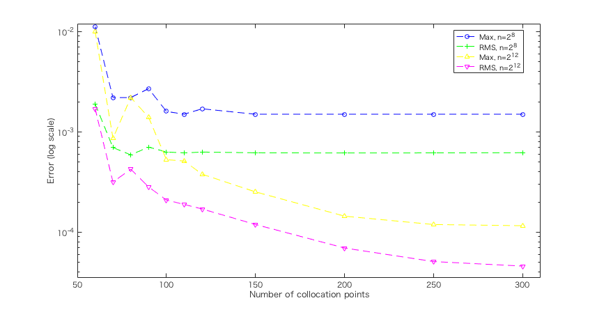
Figure 5.1: Max and RSM errors for $d=1$ with $n=2^{8},2^{12}$.

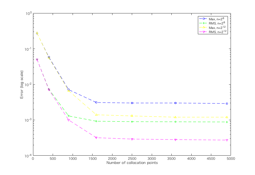
Figure 5.2: Max and RMS errors for $d=2$ with $n=2^{8},2^{12}$.

We can see that for $d=1$ with $n=2^{8}$, the curves of the both errors become flat after $N=150$. Similar phenomenons are observed in the cases of $d=2$ with $n=2^{8}$ and $n=2^{12}$. For $N$ belonging to those ranges, increasing the number of time steps give visible effects for the convergence.

As a comparison, we examine the explicit Euler finite difference method on the same collocation points where the gradient is computed by the central difference and the Dirichlet boundary condition is set to be zero. Figure 5.3 shows that the resulting ratios of Max (resp. RMS) errors for the finite difference to Max (resp. RMS) errors for our collocation method in the case of $d=1$, where the set of evaluation points is taken to be $\Gamma$ itself. We can see that our collocation method is competitive with the finite difference method with respect to Max errors and is superior to that one with respect to RMS errors under the same conditions.

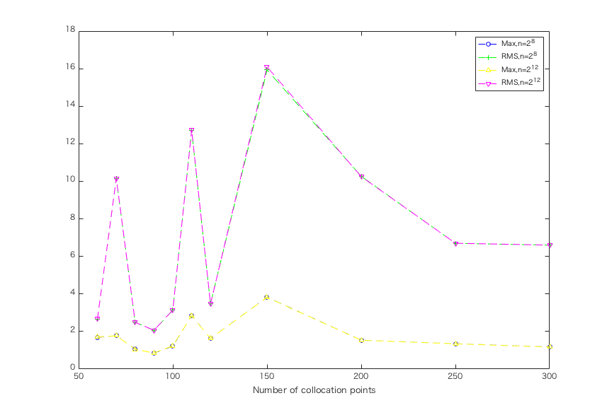
Figure 5.3: The ratios of Max and RSM errors for $d=1$ with $n=2^{8},2^{12}$.

Acknowledgements

This study is supported by JSPS KAKENHI Grant Number JP17K05359.

References

- [1] G. Barles and P. E. Souganidis. Convergence of approximation schemes for fully nonlinear second order equations. Asymptot. Anal., 4:271–283, 1991.
- [2] F. Bonnans and H. Zidani. Consistency of generalized finite difference schemes for the stochastic HJB equation. SIAM J. Numer. Anal., 41:1008–1021, 2003.
- [3] F. Camilli and M. Falcone. An approximation scheme for the optimal control of diffusion processes. Math. Model. Numer. Anal., 29:97–122, 1995.
- [4] A. Chernih, I. H. Sloan, and R. S. Womersley. Wendland functions with increasing smoothness converge to a Gaussian. Adv. Comput. Math., 40:185–200, 2014.
- [5] K. Debrabant and E. R. Jakobsen. Semi-Lagrangian schemes for linear and fully non-linear diffusion equations. Math. Comp., 82:1433–1462, 2013.
- [6] A. Fahim, N. Touzi, and X. Warin. A probabilistic numerical method for fully nonlinear parabolic PDEs. Ann. Appl. Probab., 21:1322–1364, 2011.
- [7] W. Guo, J. Zhang, and J. Zhuo. A monotone scheme for high-dimensional PDEs. Ann. Appl. Probab., 25:1540–1580, 2015.
- [8] Y. C. Hon, R. Schaback, and M. Zhong. The meshless kernel-based method of line for parabolic equations. Comput. Math. Appl., 68:2057–2067, 2014.
- [9] E. J. Kansa. Multiquadrics―a scattered data approximation scheme with application to computational fluid-dynamics―II. Computers Math. Applic., 19:147–161, 1990.
- [10] R. V. Kohn and S. Serfaty. A deterministic-control-based approach to fully nonlinear parabolic and elliptic equations. Comm. Pure Appl. Math., 63:1298–1350, 2010.
- [11] H. J. Kushner and P. Dupuis. Numerical methods for stochastic control problems in continuous time. Springer-Verlag, New York, 2001.
- [12] Y. Nakano. An approximation scheme for stochastic controls in continuous time. Jpn. J. Ind. Appl. Math., 31:681–696, 2014.
- [13] Y. Nakano. Convergence of meshfree collocation methods for fully nonlinear parabolic equations. Numer. Math., 136:703–723, 2017.
- [14] G. Pagès, H. Pham, and J. Printems. An optimal Markovian quantization algorithm for multidimensional stochastic control problems. Stoch. Dyn., 4:501–545, 2004.
- [15] H. Wendland. Scattered data approximation. Cambridge University Press, Cambridge, 2010.