On the Local Minima of the Empirical Risk

Abstract

Population risk is always of primary interest in machine learning; however, learning algorithms only have access to the empirical risk. Even for applications with nonconvex nonsmooth losses (such as modern deep networks), the population risk is generally significantly more well-behaved from an optimization point of view than the empirical risk. In particular, sampling can create many spurious local minima. We consider a general framework which aims to optimize a smooth nonconvex function $F$ (population risk) given only access to an approximation $f$ (empirical risk) that is pointwise close to $F$ (i.e., $\|{F-f}\|_{\infty}\leq\nu$). Our objective is to find the $\epsilon$-approximate local minima of the underlying function $F$ while avoiding the shallow local minima—arising because of the tolerance $\nu$—which exist only in $f$. We propose a simple algorithm based on stochastic gradient descent (SGD) on a smoothed version of $f$ that is guaranteed to achieve our goal as long as $\nu\leq O(\epsilon^{1.5}/d)$. We also provide an almost matching lower bound showing that our algorithm achieves optimal error tolerance $\nu$ among all algorithms making a polynomial number of queries of $f$. As a concrete example, we show that our results can be directly used to give sample complexities for learning a ReLU unit.

1 Introduction

The optimization of nonconvex loss functions has been key to the success of modern machine learning. While classical research in optimization focused on convex functions having a unique critical point that is both locally and globally minimal, a nonconvex function can have many local maxima, local minima and saddle points, all of which pose significant challenges for optimization. A recent line of research has yielded significant progress on one aspect of this problem—it has been established that favorable rates of convergence can be obtained even in the presence of saddle points, using simple variants of stochastic gradient descent (e.g., Ge et al., 2015; Carmon et al., 2016; Agarwal et al., 2017; Jin et al., 2017a). These research results have introduced new analysis tools for nonconvex optimization, and it is of significant interest to begin to use these tools to attack the problems associated with undesirable local minima.

It is NP-hard to avoid all of the local minima of a general nonconvex function. But there are some classes of local minima where we might expect that simple procedures—such as stochastic gradient descent—may continue to prove effective. In particular, in this paper we consider local minima that are created by small perturbations to an underlying smooth objective function. Such a setting is natural in statistical machine learning problems, where data arise from an underlying population, and the population risk, $F$, is obtained as an expectation over a continuous loss function and is hence smooth; i.e., we have $F(\bm{\theta})=\mathbb{E}_{\mathbf{z}\sim\mathcal{D}}[L(\bm{\theta};\mathbf{z})]$, for a loss function $L$ and population distribution $\mathcal{D}$. The sampling process turns this smooth risk into an empirical risk, $f(\bm{\theta})=\sum_{i=1}^{n}L(\bm{\theta};\mathbf{z}_{i})/n$, which may be nonsmooth and which generally may have many shallow local minima. From an optimization point of view $f$ can be quite poorly behaved; indeed, it has been observed in deep learning that the empirical risk may have exponentially many shallow local minima, even when the underlying population risk is well-behaved and smooth almost everywhere (Brutzkus and Globerson, 2017; Auer et al., 1996). From a statistical point of view, however, we can make use of classical results in empirical process theory (see, e.g., Boucheron et al., 2013; Bartlett and Mendelson, 2003) to show that, under certain assumptions on the sampling process, $f$ and $F$ are uniformly close:

$$\|{F-f}\|_{\infty}\leq\nu,$$ (1)

where the error $\nu$ typically decreases with the number of samples $n$. See Figure 1(a) for a depiction of this result, and Figure 1(b) for an illustration of the effect of sampling on the optimization landscape. We wish to exploit this nearness of $F$ and $f$ to design and analyze optimization procedures that find approximate local minima (see Definition 1) of the smooth function $F$, while avoiding the local minima that exist only in the sampled function $f$.

Although the relationship between population risk and empirical risk is our major motivation, we note that other applications of our framework include two-stage robust optimization and private learning (see Section 5.2). In these settings, the error $\nu$ can be viewed as the amount of adversarial perturbation or noise due to sources other than data sampling. As in the sampling setting, we hope to show that simple algorithms such as stochastic gradient descent are able to escape the local minima that arise as a function of $\nu$.

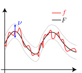
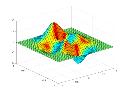
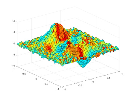
Figure 1: a) Function error $\nu$; b) Population risk vs empirical risk

Much of the previous work on this problem studies relatively small values of $\nu$, leading to “shallow” local minima, and applies relatively large amounts of noise, through algorithms such as simulated annealing (Belloni et al., 2015) and stochastic gradient Langevin dynamics (SGLD) (Zhang et al., 2017). While such “large-noise algorithms” may be justified if the goal is to approach a stationary distribution, it is not clear that such large levels of noise is necessary in the optimization setting in order to escape shallow local minima. The best existing result for the setting of nonconvex $F$ requires the error $\nu$ to be smaller than $O(\epsilon^{2}/d^{8})$, where $\epsilon$ is the precision of the optimization guarantee (see Definition 1) and $d$ is the problem dimension (Zhang et al., 2017) (see Figure 2). A fundamental question is whether algorithms exist that can tolerate a larger value of $\nu$, which would imply that they can escape “deeper” local minima. In the context of empirical risk minimization, such a result would allow fewer samples to be taken while still providing a strong guarantee on avoiding local minima.

We thus focus on the two central questions: (1) Can a simple, optimization-based algorithm avoid shallow local minima despite the lack of “large noise”? (2) Can we tolerate larger error $\nu$ in the optimization setting, thus escaping “deeper” local minima? What is the largest error that the best algorithm can tolerate?

In this paper, we answer both questions in the affirmative, establishing optimal dependencies between the error $\nu$ and the precision of a solution $\epsilon$. We propose a simple algorithm based on SGD (Algorithm 1) that is guaranteed to find an approximate local minimum of $F$ efficiently if $\nu\leq O(\epsilon^{1.5}/d)$, thus escaping all saddle points of $F$ and all additional local minima introduced by $f$. Moreover, we provide a matching lower bound (up to logarithmic factors) for all algorithms making a polynomial number of queries of $f$. The lower bound shows that our algorithm achieves the optimal tradeoff between $\nu$ and $\epsilon$, as well as the optimal dependence on dimension $d$. We also consider the information-theoretic limit for identifying an approximate local minimum of $F$ regardless of the number of queries. We give a sharp information-theoretic threshold: $\nu=\Theta(\epsilon^{1.5})$ (see Figure 2).

As a concrete example of the application to minimizing population risk, we show that our results can be directly used to give sample complexities for learning a ReLU unit, whose empirical risk is nonsmooth while the population risk is smooth almost everywhere.

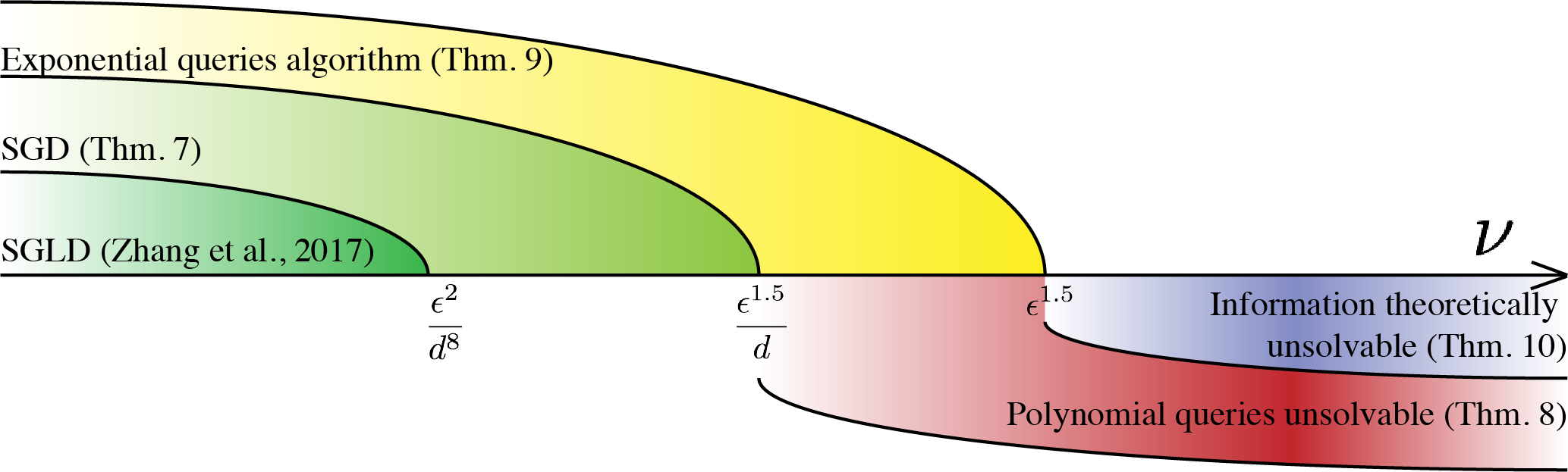
Figure 2: Complete characterization of error $\nu$ vs accuracy $\epsilon$ and dimension $d$.

1.1 Related Work

A number of other papers have examined the problem of optimizing a target function $F$ given only function evaluations of a function $f$ that is pointwise close to $F$. Belloni et al. (2015) proposed an algorithm based on simulated annealing. The work of Risteski and Li (2016) and Singer and Vondrak (2015) discussed lower bounds, though only for the setting in which the target function $F$ is convex. For nonconvex target functions $F$, Zhang et al. (2017) studied the problem of finding approximate local minima of $F$, and proposed an algorithm based on Stochastic Gradient Langevin Dynamics (SGLD) (Welling and Teh, 2011), with maximum tolerance for function error $\nu$ scaling as $O(\epsilon^{2}/d^{8})$. Other than difference in algorithm style and $\nu$ tolerance as shown in Figure 2, we also note that we do not require regularity assumptions on top of smoothness, which are inherently required by the MCMC algorithm proposed in Zhang et al. (2017). Finally, we note that in parallel, Kleinberg et al. (2018) solved a similar problem using SGD under the assumption that $F$ is one-point convex.

Previous work has also studied the relation between the landscape of empirical risks and the landscape of population risks for nonconvex functions. Mei et al. (2016) examined a special case where the individual loss functions $L$ are also smooth, which under some assumptions implies uniform convergence of the gradient and Hessian of the empirical risk to their population versions. Loh and Wainwright (2013) showed for a restricted class of nonconvex losses that even though many local minima of the empirical risk exist, they are all close to the global minimum of population risk.

Our work builds on recent work in nonconvex optimization, in particular, results on escaping saddle points and finding approximate local minima. Beyond the classical result by Nesterov (2004) for finding first-order stationary points by gradient descent, recent work has given guarantees for escaping saddle points by gradient descent (Jin et al., 2017a) and stochastic gradient descent (Ge et al., 2015). Agarwal et al. (2017) and Carmon et al. (2016) established faster rates using algorithms that make use of Nesterov’s accelerated gradient descent in a nested-loop procedure (Nesterov, 1983), and Jin et al. (2017b) have established such rates even without the nested loop. There have also been empirical studies on various types of local minima (e.g. Keskar et al., 2016; Dinh et al., 2017).

Finally, our work is also related to the literature on zero-th order optimization or more generally, bandit convex optimization. Our algorithm uses function evaluations to construct a gradient estimate and perform SGD, which is similar to standard methods in this community (e.g., Flaxman et al., 2005; Agarwal et al., 2010; Duchi et al., 2015). Compared to first-order optimization, however, the convergence of zero-th order methods is typically much slower, depending polynomially on the underlying dimension even in the convex setting (Shamir, 2013). Other derivative-free optimization methods include simulated annealing (Kirkpatrick et al., 1983) and evolutionary algorithms (Rechenberg and Eigen, 1973), whose convergence guarantees are less clear.

2 Preliminaries

Notation

We use bold lower-case letters to denote vectors, as in $\mathbf{x},\mathbf{y},\mathbf{z}$. We use $\|{\cdot}\|$ to denote the $\ell_{2}$ norm of vectors and spectral norm of matrices. For a matrix, $\lambda_{\min}$ denotes its smallest eigenvalue. For a function $f:\mathbb{R}^{d}\to\mathbb{R}$, $\nabla f$ and $\nabla^{2}f$ denote its gradient vector and Hessian matrix respectively. We also use $\|{\cdot}\|_{\infty}$ on a function $f$ to denote the supremum of its absolute function value over entire domain, $\sup_{\mathbf{x}\in\mathbb{R}^{d}}|f|$. We use $\mathbb{B}_{0}(r)$ to denote the $\ell_{2}$ ball of radius $r$ centered at $0$ in $\mathbb{R}^{d}$. We use notation $\tilde{O}(\cdot),\tilde{\Theta}(\cdot),\tilde{\Omega}(\cdot)$ to hide only absolute constants and poly-logarithmic factors. A multivariate Gaussian distribution with mean $\bm{0}$ and covariance $\sigma^{2}$ in every direction is denoted as $\mathcal{N}(\bm{0},\sigma^{2}\bm{I})$. Throughout the paper, we say “polynomial number of queries” to mean that the number of queries depends polynomially on all problem-dependent parameters.

Objectives in nonconvex optimization

Our goal is to find a point that has zero gradient and positive semi-definite Hessian, thus escaping saddle points. We formalize this idea as follows.

Definition 1.

$\mathbf{x}$ is called a second-order stationary point (SOSP) or approximate local minimum of a function $F$ if

$$\|{\nabla F(\mathbf{x})}\|=0\text{~{}and~{}}\lambda_{\min}(\nabla^{2}F(\mathbf{x}))\geq 0.$$

We note that there is a slight difference between SOSP and local minima—an SOSP as defined here does not preclude higher-order saddle points, which themselves can be NP-hard to escape from (Anandkumar and Ge, 2016).

Since an SOSP is characterized by its gradient and Hessian, and since convergence of algorithms to an SOSP will depend on these derivatives in a neighborhood of an SOSP, it is necessary to impose smoothness conditions on the gradient and Hessian. A minimal set of conditions that have become standard in the literature are the following.

Definition 2.

A function $F$ is $\ell$-gradient Lipschitz if $~{}\forall\mathbf{x},\mathbf{y}~{}~{}\|{\nabla F(\mathbf{x})-\nabla F(\mathbf{y})}\|\leq\ell\|{\mathbf{x}-\mathbf{y}}\|.$

Definition 3.

A function $F$ is $\rho$-Hessian Lipschitz if $~{}\forall\mathbf{x},\mathbf{y}~{}~{}\|{\nabla^{2}F(\mathbf{x})-\nabla^{2}F(\mathbf{y})}\|\leq\rho\|{\mathbf{x}-\mathbf{y}}\|.$

Another common assumption is that the function is bounded.

Definition 4.

A function $F$ is $B$-bounded if for any $\mathbf{x}$ that $|F(\mathbf{x})|\leq B$.

For any finite-time algorithm, we cannot hope to find an exact SOSP. Instead, we can define $\epsilon$-approximate SOSP that satisfy relaxations of the first- and second-order optimality conditions. Letting $\epsilon$ vary allows us to obtain rates of convergence.

Definition 5.

$\mathbf{x}$ is an $\epsilon$-second-order stationary point ($\epsilon$-SOSP) of a $\rho$-Hessian Lipschitz function $F$ if

$$\|{\nabla F(\mathbf{x})}\|\leq\epsilon\text{~{}and~{}}\lambda_{\min}(\nabla^{2}F(\mathbf{x}))\geq-\sqrt{\rho\epsilon}.$$

Given these definitions, we can ask whether it is possible to find an $\epsilon$-SOSP in polynomial time under the Lipchitz properties. Various authors have answered this question in the affirmative.

Theorem 6.

(e.g. Carmon et al., 2016; Agarwal et al., 2017; Jin et al., 2017a) If the function $F:\mathbb{R}^{d}\to\mathbb{R}$ is $B$-bounded, $l$-gradient Lipschitz and $\rho$ Hessian Lipschitz, given access to the gradient (and sometimes Hessian) of $F$, it is possible to find an $\epsilon$-SOSP in $\mbox{poly}(d,B,l,\rho,1/\epsilon)$ time.

3 Main Results

In the setting we consider, there is an unknown function $F$ (the population risk) that has regularity properties (bounded, gradient and Hessian Lipschitz). However, we only have access to a function $f$ (the empirical risk) that may not even be everywhere differentiable. The only information we use is that $f$ is pointwise close to $F$. More precisely, we assume

Assumption A1.

We assume that the function pair ($F:\mathbb{R}^{d}\to\mathbb{R},f:\mathbb{R}^{d}\to\mathbb{R}$) satisfies the following properties:

1. $F$ is $B$-bounded, $\ell$-gradient Lipschitz, $\rho$-Hessian Lipschitz.

2. $f,F$ are $\nu$-pointwise close; i.e., $\|F-f\|_{\infty}\leq\nu$.

As we explained in Section 2, our goal is to find second-order stationary points of $F$ given only function value access to $f$. More precisely:

Problem 1.

Given a function pair ($F,f$) that satisfies Assumption A1, find an $\epsilon$-second-order stationary point of $F$ with only access to values of $f$.

The only way our algorithms are allowed to interact with $f$ is to query a point $\mathbf{x}$, and obtain a function value $f(\mathbf{x})$. This is usually called a zero-th order oracle in the optimization literature. In this paper we give tight upper and lower bounds for the dependencies between $\nu$, $\epsilon$ and $d$, both for algorithms with polynomially many queries and in the information-theoretic limit.

3.1 Optimal algorithm with polynomial number of queries

There are three main difficulties in applying stochastic gradient descent to Problem 1: (1) in order to converge to a second-order stationary point of $F$, the algorithm must avoid being stuck in saddle points; (2) the algorithm does not have access to the gradient of $f$; (3) there is a gap between the observed $f$ and the target $F$, which might introduce non-smoothness or additional local minima. The first difficulty was addressed in Jin et al. (2017a) by perturbing the iterates in a small ball; this pushes the iterates away from any potential saddle points. For the latter two difficulties, we apply Gaussian smoothing to $f$ and use $\mathbf{z}[f(\mathbf{x}+\mathbf{z})-f(\mathbf{x})]/\sigma^{2}$ ($\mathbf{z}\sim\mathcal{N}(0,\sigma^{2}\mathbf{I})$) as a stochastic gradient estimate. This estimate, which only requires function values of $f$, is well known in the zero-th order optimization literature (e.g. Duchi et al., 2015). For more details, see Section 4.1.

Algorithm 1 Zero-th order Perturbed Stochastic Gradient Descent (ZPSGD)

0:  $\mathbf{x}_{0}$, learning rate $\eta$, noise radius $r$, mini-batch size $m$.

  for $t=0,1,\ldots,$ do

     sample $(\mathbf{z}^{(1)}_{t},\cdots,\mathbf{z}^{(m)}_{t})\sim\mathcal{N}(0,\sigma^{2}\mathbf{I})$

     $\mathbf{g}_{t}(\mathbf{x}_{t})\leftarrow\sum_{i=1}^{m}\mathbf{z}^{(i)}_{t}[f(\mathbf{x}_{t}+\mathbf{z}^{(i)}_{t})-f(\mathbf{x}_{t})]/(m\sigma^{2})$

     $\mathbf{x}_{t+1}\leftarrow\mathbf{x}_{t}-\eta(\mathbf{g}_{t}(\mathbf{x}_{t})+\xi_{t}),\qquad\xi_{t}\text{~{}uniformly~{}}\sim\mathbb{B}_{0}(r)$

  return $\mathbf{x}_{T}$

In short, our algorithm (Algorithm 1) is a variant of SGD, which uses $\mathbf{z}[f(\mathbf{x}+\mathbf{z})-f(\mathbf{x})]/\sigma^{2}$ as the gradient estimate (computed over mini-batches), and adds isotropic perturbations. Using this algorithm, we can achieve the following trade-off between $\nu$ and $\epsilon$.

Theorem 7 (Upper Bound (ZPSGD)).

Given that the function pair ($F,f$) satisfies Assumption A1 with $\nu\leq O(\sqrt{\epsilon^{3}/\rho}\cdot(1/d))$, then for any $\delta>0$, with smoothing parameter $\sigma=\Theta(\sqrt{\epsilon/(\rho d)})$, learning rate $\eta=1/\ell$, perturbation $r=\tilde{\Theta}(\epsilon)$, and mini-batch size $m=\text{poly}(d,B,\ell,\rho,1/\epsilon,\log(1/\delta))$, ZPSGD will find an $\epsilon$-second-order stationary point of $F$ with probability $1-\delta$, in $\text{poly}(d,B,\ell,\rho,1/\epsilon,\log(1/\delta))$ number of queries.

Theorem 7 shows that assuming a small enough function error $\nu$, ZPSGD will solve Problem 1 within a number of queries that is polynomial in all the problem-dependent parameters. The tolerance on function error $\nu$ varies inversely with the number of dimensions, $d$. This rate is in fact optimal for all polynomial queries algorithms. In the following result, we show that the $\epsilon,\rho,$ and $d$ dependencies in function difference $\nu$ are tight up to a logarithmic factors in $d$.

Theorem 8 (Polynomial Queries Lower Bound).

For any $B>0,\ell>0,\rho>0$ there exists $\epsilon_{0}=\Theta(\min\{\ell^{2}/\rho,(B^{2}\rho/d^{2})^{1/3}\})$ such that for any $\epsilon\in(0,\epsilon_{0}]$, there exists a function pair ($F,f$) satisfying Assumption A1 with $\nu=\tilde{\Theta}(\sqrt{\epsilon^{3}/\rho}\cdot(1/d))$, so that any algorithm that only queries a polynomial number of function values of $f$ will fail, with high probability, to find an $\epsilon$-SOSP of $F$.

This theorem establishes that for any $\rho,\ell,B$ and any $\epsilon$ small enough, we can construct a randomized ‘hard’ instance ($F,f$) such that any (possibly randomized) algorithm with a polynomial number of queries will fail to find an $\epsilon$-SOSP of $F$ with high probability. Note that the error $\nu$ here is only a poly-logarithmic factor larger than the requirement for our algorithm. In other words, the guarantee of our Algorithm 1 in Theorem 7 is optimal up to a logarithmic factor.

3.2 Information-theoretic guarantees

If we allow an unlimited number of queries, we can show that the upper and lower bounds on the function error tolerance $\nu$ no longer depends on the problem dimension $d$. That is, Problem 1 exhibits a statistical-computational gap—polynomial-queries algorithms are unable to achieve the information-theoretic limit. We first state that an algorithm (with exponential queries) is able to find an $\epsilon$-SOSP of $F$ despite a much larger value of error $\nu$. The basic algorithmic idea is that an $\epsilon$-SOSP must exist within some compact space, such that once we have a subroutine that approximately computes the gradient and Hessian of $F$ at an arbitrary point, we can perform a grid search over this compact space (see Section D for more details):

Theorem 9.

There exists an algorithm so that if the function pair ($F,f$) satisfies Assumption A1 with $\nu\leq O(\sqrt{\epsilon^{3}/\rho})$ and $\ell>\sqrt{\rho\epsilon}$, then the algorithm will find an $\epsilon$-second-order stationary point of $F$ with an exponential number of queries.

We also show a corresponding information-theoretic lower bound that prevents any algorithm from even identifying a second-order stationary point of $F$. This completes the characterization of function error tolerance $\nu$ in terms of required accuracy $\epsilon$.

Theorem 10.

For any $B>0,\ell>0,\rho>0$, there exists $\epsilon_{0}=\Theta(\min\{\ell^{2}/\rho,(B^{2}\rho/d)^{1/3}\})$ such that for any $\epsilon\in(0,\epsilon_{0}]$ there exists a function pair ($F,f$) satisfying Assumption A1 with $\nu=O(\sqrt{\epsilon^{3}/\rho})$, so that any algorithm will fail, with high probability, to find an $\epsilon$-SOSP of $F$.

3.3 Extension: Gradients pointwise close

We may extend our algorithmic ideas to solve the problem of optimizing an unknown smooth function $F$ when given only a gradient vector field $\mathbf{g}:\mathbb{R}^{d}\to\mathbb{R}^{d}$ that is pointwise close to the gradient $\nabla F$. Specifically, we answer the question: what is the error in the gradient oracle that we can tolerate to obtain optimization guarantees for the true function $F$? We observe that our algorithm’s tolerance on gradient error is much better compared to Theorem 7. Details can be found in Appendix E and F.

4 Overview of Analysis

In this section we present the key ideas underlying our theoretical results. We will focus on the results for algorithms that make a polynomial number of queries (Theorems 7 and 8).

4.1 Efficient algorithm for Problem 1

We first argue the correctness of Theorem 7. As discussed earlier, there are two key ideas in the algorithm: Gaussian smoothing and perturbed stochastic gradient descent. Gaussian smoothing allows us to transform the (possibly non-smooth) function $f$ into a smooth function $\tilde{f}_{\sigma}$ that has similar second-order stationary points as $F$; at the same time, it can also convert function evaluations of $f$ into a stochastic gradient of $\tilde{f}_{\sigma}$. We can use this stochastic gradient information to find a second-order stationary point of $\tilde{f}_{\sigma}$, which by the choice of the smoothing radius is guaranteed to be an approximate second-order stationary point of $F$.

First, we introduce Gaussian smoothing, which perturbs the current point $\mathbf{x}$ using a multivariate Gaussian and then takes an expectation over the function value.

Definition 11 (Gaussian smoothing).

Given $f$ satisfying assumption A1, define its Gaussian smoothing as $\tilde{f}_{\sigma}(\mathbf{x})=\mathbb{E}_{\mathbf{z}\sim\mathcal{N}(0,\sigma^{2}\mathbf{I})}[f(\mathbf{x}+\mathbf{z})]$. The parameter $\sigma$ is henceforth called the smoothing radius.

In general $f$ need not be smooth or even differentiable, but its Gaussian smoothing $\tilde{f}_{\sigma}$ will be a differentiable function. Although it is in general difficult to calculate the exact smoothed function $\tilde{f}_{\sigma}$, it is not hard to give an unbiased estimate of function value and gradient of $\tilde{f}_{\sigma}$:

Lemma 12.

(e.g. Duchi et al., 2015) Let $\tilde{f}_{\sigma}$ be the Gaussian smoothing of $f$ (as in Definition 11), the gradient of $\tilde{f}_{\sigma}$ can be computed as $~{}\nabla\tilde{f}_{\sigma}=\frac{1}{\sigma^{2}}\mathbb{E}_{\mathbf{z}\sim\mathcal{N}(0,\sigma^{2}\mathbf{I})}[(f(\mathbf{x}+\mathbf{z})-f(\mathbf{x}))\mathbf{z}].$

Lemma 12 allows us to query the function value of $f$ to get an unbiased estimate of the gradient of $\tilde{f}_{\sigma}$. This stochastic gradient is used in Algorithm 1 to find a second-order stationary point of $\tilde{f}_{\sigma}$.

To make sure the optimizer is effective on $\tilde{f}_{\sigma}$ and that guarantees on $\tilde{f}_{\sigma}$ carry over to the target function $F$, we need two sets of properties: the smoothed function $\tilde{f}_{\sigma}$ should be gradient and Hessian Lipschitz, and at the same time should have gradients and Hessians close to those of the true function $F$. These properties are summarized in the following lemma:

Lemma 13 (Property of smoothing).

Assume that the function pair ($F,f$) satisfies Assumption A1, and let $\tilde{f}_{\sigma}(\mathbf{x})$ be as given in definition 11. Then, the following holds

1. $\tilde{f}_{\sigma}(\mathbf{x})$ is $O(\ell+\frac{\nu}{\sigma^{2}})$-gradient Lipschitz and $O(\rho+\frac{\nu}{\sigma^{3}})$-Hessian Lipschitz.

2. $\|{\nabla\tilde{f}_{\sigma}(\mathbf{x})-\nabla F(\mathbf{x})}\|\leq O(\rho d\sigma^{2}+\frac{\nu}{\sigma})$ and $\|{\nabla^{2}\tilde{f}_{\sigma}(\mathbf{x})-\nabla^{2}F(\mathbf{x})}\|\leq O(\rho\sqrt{d}\sigma+\frac{\nu}{\sigma^{2}})$.

The proof is deferred to Appendix A. Part (1) of the lemma says that the gradient (and Hessian) Lipschitz constants of $\tilde{f}_{\sigma}$ are similar to the gradient (and Hessian) Lipschitz constants of $F$ up to a term involving the function difference $\nu$ and the smoothing parameter $\sigma$. This means as $f$ is allowed to deviate further from $F$, we must smooth over a larger radius—choose a larger $\sigma$—to guarantee the same smoothness as before. On the other hand, part (2) implies that choosing a large $\sigma$ increases the upper bound on the gradient and Hessian difference between $\tilde{f}_{\sigma}$ and $F$. Smoothing is a form of local averaging, so choosing a too-large radius will erase information about local geometry. The choice of $\sigma$ must strike the right balance between making $\tilde{f}_{\sigma}$ smooth (to guarantee ZPSGD finds a $\epsilon$-SOSP of $\tilde{f}_{\sigma}$ ) and keeping the derivatives of $\tilde{f}_{\sigma}$ close to those of $F$ (to guarantee any $\epsilon$-SOSP of $\tilde{f}_{\sigma}$ is also an $O(\epsilon)$-SOSP of $F$). In Appendix A.3, we show that this can be satisfied by choosing $\sigma=\sqrt{\epsilon/(\rho d)}$.

Perturbed stochastic gradient descent

In ZPSGD, we use the stochastic gradients suggested by Lemma 12. Perturbed Gradient Descent (PGD) (Jin et al., 2017a) was shown to converge to a second-order stationary point. Here we use a simple modification of PGD that relies on batch stochastic gradient. In order for PSGD to converge, we require that the stochastic gradients are well-behaved; that is, they are unbiased and have good concentration properties, as asserted in the following lemma. It is straightforward to verify given that we sample $\mathbf{z}$ from a zero-mean Gaussian (proof in Appendix A.2).

Lemma 14 (Property of stochastic gradient).

Let $\mathbf{g}(\mathbf{x};\mathbf{z})=\mathbf{z}[f(\mathbf{x}+\mathbf{z})-f(\mathbf{x})]/\sigma^{2}$, where $\mathbf{z}\sim\mathcal{N}(0,\sigma^{2}\mathbf{I})$. Then $\mathbb{E}_{\mathbf{z}}\mathbf{g}(\mathbf{x};\mathbf{z})=\nabla\tilde{f}_{\sigma}(\mathbf{x})$, and $\mathbf{g}(\mathbf{x};\mathbf{z})$ is sub-Gaussian with parameter $\frac{B}{\sigma}$.

As it turns out, these assumptions suffice to guarantee that perturbed SGD (PSGD), a simple adaptation of PGD in Jin et al. (2017a) with stochastic gradient and large mini-batch size, converges to the second-order stationary point of the objective function.

Theorem 15 (PSGD efficiently escapes saddle points (Jin et al., 2018), informal).

Suppose $f(\cdot)$ is $\ell$-gradient Lipschitz and $\rho$-Hessian Lipschitz, and stochastic gradient $\mathbf{g}(\mathbf{x},\theta)$ with $\mathbb{E}\mathbf{g}(\mathbf{x};\theta)=\nabla f(\mathbf{x})$ has a sub-Gaussian tail with parameter $\sigma/\sqrt{d}$, then for any $\delta>0$, with proper choice of hyperparameters, PSGD (Algorithm 4) will find an $\epsilon$-SOSP of $f$ with probability $1-\delta$, in $\text{poly}(d,B,\ell,\rho,\sigma,1/\epsilon,\log(1/\delta))$ number of queries.

For completeness, we include the formal version of the theorem and its proof in Appendix H. Combining this theorem and the second part of Lemma 13, we see that by choosing an appropriate smoothing radius $\sigma$, our algorithm ZPSGD finds an $C\epsilon/\sqrt{d}$-SOSP for $\tilde{f}_{\sigma}$ which is also an $\epsilon$-SOSP for $F$ for some universal constant $C$.

4.2 Polynomial queries lower bound

The proof of Theorem 8 depends on the construction of a ‘hard’ function pair. The argument crucially depends on the concentration of measure in high dimensions. We provide a proof sketch in Appendix B and the full proof in Appendix C.

5 Applications

In this section, we present several applications of our algorithm. We first show a simple example of learning one rectified linear unit (ReLU), where the empirical risk is nonconvex and nonsmooth. We also briefly survey other potential applications for our model as stated in Problem 1.

5.1 Statistical Learning Example: Learning ReLU

Consider the simple example of learning a ReLU unit. Let $\text{ReLU}(z)=\max\{z,0\}$ for $z\in\mathbb{R}$. Let $\mathbf{w}^{\star}(\|{\mathbf{w}^{\star}}\|=1)$ be the desired solution. We assume data $(\mathbf{x}_{i},\mathbf{y}_{i})$ is generated as $y_{i}=\text{ReLU}(\mathbf{x}_{i}^{\top}\mathbf{w}^{\star})+\zeta_{i}$ where noise $\zeta_{i}\sim\mathcal{N}(0,1)$. We further assume the features $\mathbf{x}_{i}\sim\mathcal{N}(0,\mathbf{I})$ are also generated from a standard Gaussian distribution. The empirical risk with a squared loss function is:

$$\hat{R}_{n}(\mathbf{w})=\frac{1}{n}\sum_{i=1}^{n}(y_{i}-\text{ReLU}(\mathbf{x}_{i}^{\top}\mathbf{w}))^{2}.$$

Its population version is $R(\mathbf{w})=\mathbb{E}[\hat{R}_{n}(\mathbf{w})]$. In this case, the empirical risk is highly nonsmooth—in fact, not differentiable in all subspaces perpendicular to each $\mathbf{x}_{i}$. The population risk turns out to be smooth in the entire space $\mathbb{R}^{d}$ except at $\bm{0}$. This is illustrated in Figure 3, where the empirical risk displays many sharp corners.

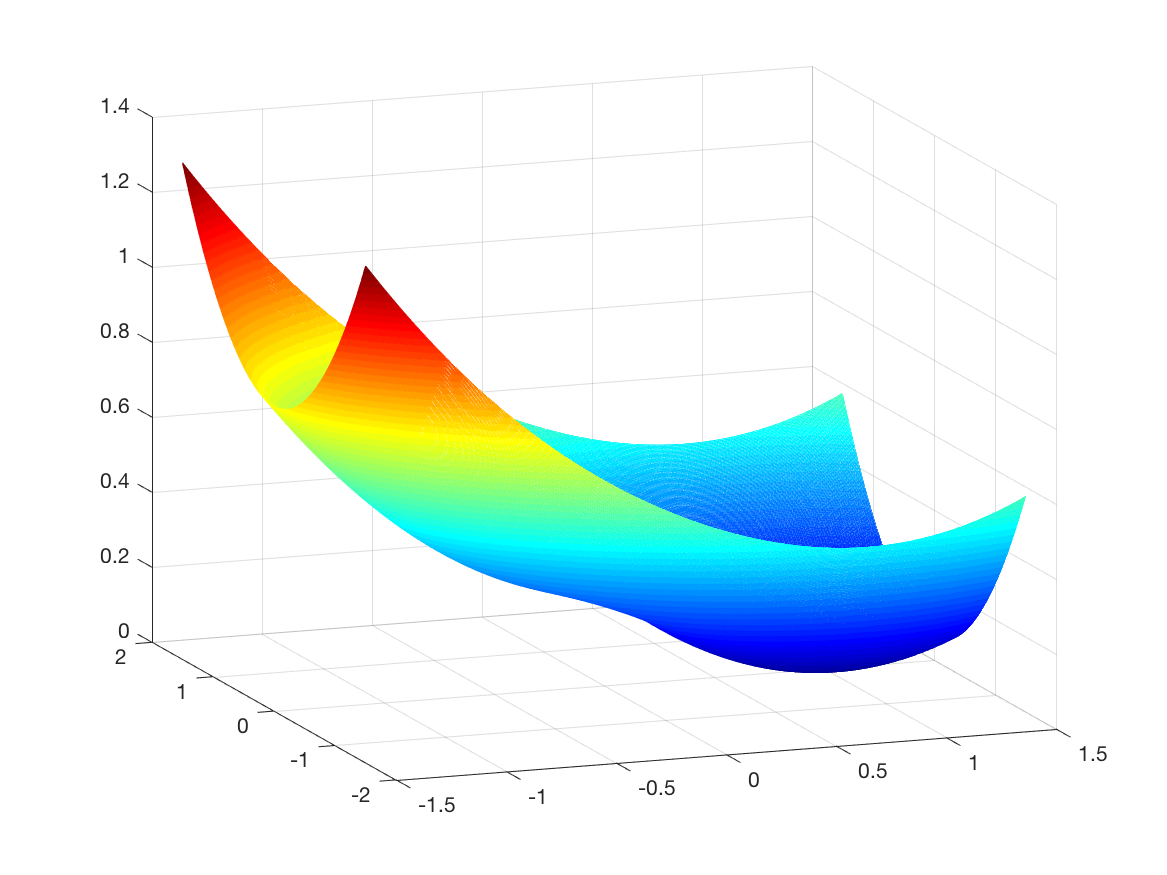
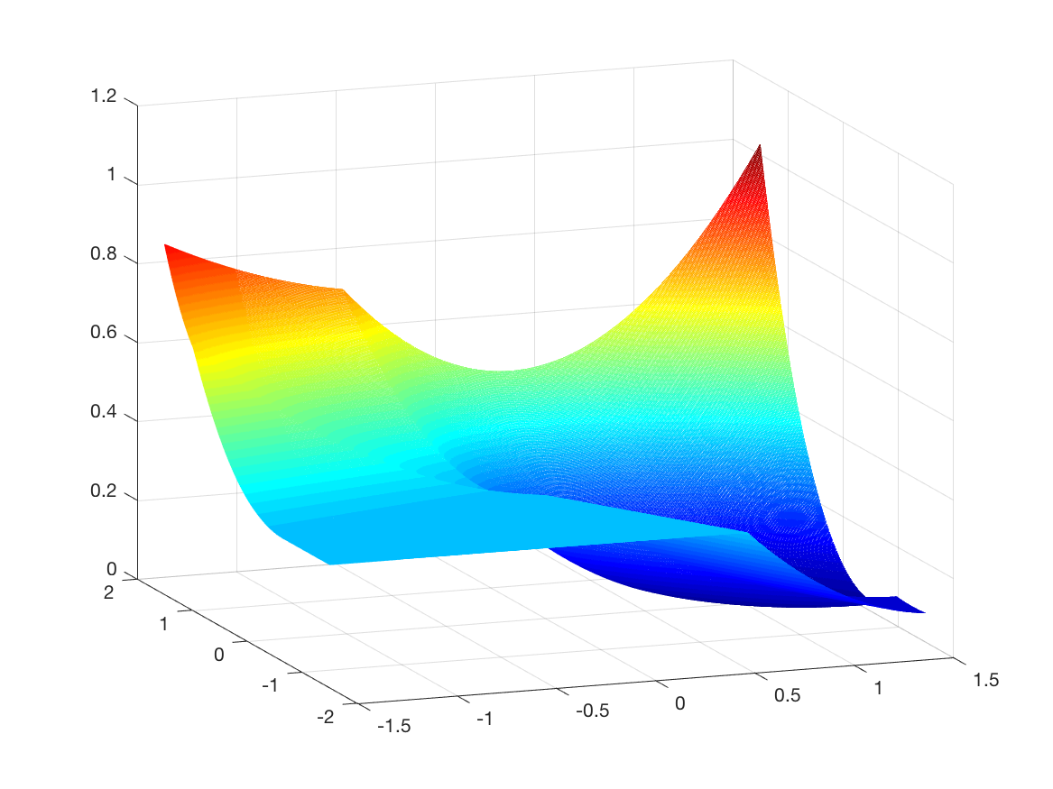
Figure 3: Population (left) and Empirical (right) risk for learning ReLU Unit , $d=2$. Sharp corners present in the empirical risk are not found in the population version.

Due to nonsmoothness at $\bm{0}$ even for population risk, we focus on a compact region $\mathfrak{B}=\{\mathbf{w}|\mathbf{w}^{\top}\mathbf{w}^{\star}\geq\frac{1}{\sqrt{d}}\}\cap\{\mathbf{w}|\|{\mathbf{w}}\|\leq 2\}$ which excludes $\bm{0}$. This region is large enough so that a random initialization has at least constant probability of being inside it. We also show the following properties that allow us to apply Algorithm 1 directly:

Lemma 16.

The population and empirical risk $R,\hat{R}_{n}$ of learning a ReLU unit problem satisfies:
1. If $\mathbf{w}_{0}\in\mathfrak{B}$, then runing ZPSGD (Algorithm 1) gives $\mathbf{w}_{t}\in\mathfrak{B}$ for all $t$ with high probability.
2. Inside $\mathfrak{B}$, $R$ is $O(1)$-bounded, $O(\sqrt{d})$-gradient Lipschitz, and $O(d)$-Hessian Lipschitz.
3. $\sup_{\mathbf{w}\in\mathfrak{B}}|\hat{R}_{n}(\mathbf{w})-R(\mathbf{w})|\leq\tilde{O}(\sqrt{d/n})$ w.h.p.
4. Inside $\mathfrak{B}$, $R$ is nonconvex function, $\mathbf{w}^{\star}$ is the only SOSP of $R(\mathbf{w})$.

These properties show that the population loss has a well-behaved landscape, while the empirical risk is pointwise close. This is exactly what we need for Algorithm 1. Using Theorem 7 we immediately get the following sample complexity, which guarantees an approximate population risk minimizer. We defer all proofs to Appendix G.

Theorem 17.

For learning a ReLU unit problem, suppose the sample size is $n\geq\tilde{O}(d^{4}/\epsilon^{3})$, and the initialization is $\mathbf{w}_{0}\sim\mathcal{N}(0,\frac{1}{d}\mathbf{I})$, then with at least constant probability, Algorithm 1 will output an estimator $\hat{\mathbf{w}}$ so that $\|{\hat{\mathbf{w}}-\mathbf{w}^{\star}}\|\leq\epsilon$.

5.2 Other applications

Private machine learning

Data privacy is a significant concern in machine learning as it creates a trade-off between privacy preservation and successful learning. Previous work on differentially private machine learning (e.g. Chaudhuri et al., 2011) have studied objective perturbation, that is, adding noise to the original (convex) objective and optimizing this perturbed objective, as a way to simultaneously guarantee differential privacy and learning generalization: $f=F+p(\varepsilon)$. Our results may be used to extend such guarantees to nonconvex objectives, characterizing when it is possible to optimize $F$ even if the data owner does not want to reveal the true value of $F(\mathbf{x})$ and instead only reveals $f(\mathbf{x})$ after adding a perturbation $p(\varepsilon)$, which depends on the privacy guarantee $\varepsilon$.

Two stage robust optimization

Motivated by the problem of adversarial examples in machine learning, there has been a lot of recent interest (e.g. Steinhardt et al., 2017; Sinha et al., 2018) in a form of robust optimization that involves a minimax problem formulation: $\min_{\mathbf{x}}\max_{\mathbf{u}}G(\mathbf{x},\mathbf{u}).$ The function $F(\mathbf{x})=\max_{\mathbf{u}}G(\mathbf{x},\mathbf{u})$ tends to be nonconvex in such problems, since $G$ can be very complicated. It can be intractable or costly to compute the solution to the inner maximization exactly, but it is often possible to get a good enough approximation $f$, such that $\sup_{\mathbf{x}}|F(\mathbf{x})-f(\mathbf{x})|=\nu$. It is then possible to solve $\min_{\mathbf{x}}f(\mathbf{x})$ by ZPSGD, with guarantees for the original optimization problem.

Acknowledgments

We thank Aditya Guntuboyina, Yuanzhi Li, Yi-An Ma, Jacob Steinhardt, and Yang Yuan for valuable discussions.

Appendix A Efficient algorithm for optimizing the population risk

As we described in Section 4, in order to find a second-order stationary point of the population loss $F$, we apply perturbed stochastic gradient on a smoothed version of the empirical loss $f$. Recall that the smoothed function is defined as

$$\tilde{f}_{\sigma}(\mathbf{x})=\mathbb{E}_{\mathbf{z}}f(\mathbf{x}+\mathbf{z}).$$

In this section we will also consider a smoothed version of the population loss $F$, as follows:

$$\tilde{F}_{\sigma}(\mathbf{x})=\mathbb{E}_{\mathbf{z}}F(\mathbf{x}+\mathbf{z}).$$

This function is of course not accessible by the algorithm and we only use it in the proof of convergence rates.

This section is organized as follows. In section A.1, we present and prove the key lemma on the properties of the smoothed function $\tilde{f}_{\sigma}(\mathbf{x})$. Next, in section A.2, we prove the properties of the stochastic gradient $\mathbf{g}$. Combining the lemmas in these two subsections, in section A.3 we prove a main theorem about the guarantees of ZPSGD (Theorem 7). For clarity, we defer all technical lemmas and their proofs to section A.4.

A.1 Properties of the Gaussian smoothing

In this section, we show the properties of smoothed function $\tilde{f}_{\sigma}(\mathbf{x})$. We first restate Lemma 13.

Lemma 18 (Property of smoothing).

Assume that the function pair ($F,f$) satisfies Assumption A1, and let $\tilde{f}_{\sigma}(\mathbf{x})$ be as given in definition 11. Then, the following holds

1. $\tilde{f}_{\sigma}(\mathbf{x})$ is $O(\ell+\frac{\nu}{\sigma^{2}})$-gradient Lipschitz and $O(\rho+\frac{\nu}{\sigma^{3}})$-Hessian Lipschitz.

2. $\|{\nabla\tilde{f}_{\sigma}(\mathbf{x})-\nabla F(\mathbf{x})}\|\leq O(\rho d\sigma^{2}+\frac{\nu}{\sigma})$ and $\|{\nabla^{2}\tilde{f}_{\sigma}(\mathbf{x})-\nabla^{2}F(\mathbf{x})}\|\leq O(\rho\sqrt{d}\sigma+\frac{\nu}{\sigma^{2}})$.

Intuitively, the first property states that if the original function $F$ is gradient and Hessian Lipschitz, the smoothed version of the perturbed function $f$ is also gradient and Hessian Lipschitz (note that this is of course not true for the perturbed function $f$); the second property shows that the gradient and Hessian of $\tilde{f}_{\sigma}$ is point-wise close to the gradient and Hessian of the original function $F$. We will prove the four points (1 and 2, gradient and Hessian) of the lemma one by one, in Sections A.1.1 to A.1.4.

In the proof, we frequently require the following lemma (see e.g. Zhang et al. (2017)) that gives alternative expressions for the gradient and Hessian of a smoothed function.

Lemma 19 (Gaussian smoothing identities (Zhang et al., 2017)).

$\tilde{f}_{\sigma}$ has gradient and Hessian:

$$\nabla\tilde{f}_{\sigma}(\mathbf{x})=\mathbb{E}_{\mathbf{z}}[\frac{\mathbf{z}}{\sigma^{2}}f(\mathbf{x}+\mathbf{z})],\quad\nabla^{2}\tilde{f}_{\sigma}(\mathbf{x})=\mathbb{E}_{\mathbf{z}}[\frac{\mathbf{z}\mathbf{z}^{\top}-\sigma^{2}\mathbf{I}}{\sigma^{4}}f(\mathbf{x}+\mathbf{z})].$$

Proof.

Using the density function of a multivariate Gaussian, we may compute the gradient of the smoothed function as follows:

$$\nabla\tilde{f}_{\sigma}(\mathbf{x}) =\frac{\partial}{\partial\mathbf{x}}\frac{1}{(2\pi\sigma^{2})^{d/2}}\int f(\mathbf{x}+\mathbf{z})e^{-\|{\mathbf{z}}\|^{2}/2\sigma^{2}}d\mathbf{z}=\frac{1}{(2\pi\sigma^{2})^{d/2}}\int\frac{\partial}{\partial\mathbf{x}}f(\mathbf{x}+\mathbf{z})e^{-\|{\mathbf{z}}\|^{2}/2\sigma^{2}}d\mathbf{z}$$

$$=\frac{1}{(2\pi\sigma^{2})^{d/2}}\int\frac{\partial}{\partial\mathbf{x}}f(\mathbf{z})e^{-\|{\mathbf{z}-\mathbf{x}}\|^{2}/2\sigma^{2}}d\mathbf{z}=\frac{1}{(2\pi\sigma^{2})^{d/2}}\int f(\mathbf{z}^{\prime})\frac{\mathbf{x}-\mathbf{z}}{\sigma^{2}}e^{-\|{\mathbf{z}-\mathbf{x}}\|^{2}/2\sigma^{2}}d\mathbf{z}$$

$$=\frac{1}{(2\pi\sigma^{2})^{d/2}}\int f(\mathbf{z}+\mathbf{x})\frac{\mathbf{z}}{\sigma^{2}}e^{-\|{-\mathbf{z}}\|^{2}/2\sigma^{2}}d\mathbf{z}=\mathbb{E}_{\mathbf{z}}[\frac{\mathbf{z}}{\sigma^{2}}f(\mathbf{x}+\mathbf{z})],$$

and similarly, we may compute the Hessian of the smoothed function:

$$\nabla^{2}\tilde{f}_{\sigma}(\mathbf{x}) =\frac{\partial}{\partial\mathbf{x}}\frac{1}{(2\pi\sigma^{2})^{d/2}}\int\frac{\mathbf{z}}{\sigma^{2}}f(\mathbf{x}+\mathbf{z})e^{-\|{\mathbf{z}}\|^{2}/2\sigma^{2}}d\mathbf{z}$$

$$=\frac{1}{(2\pi\sigma^{2})^{d/2}}\int\frac{\partial}{\partial\mathbf{x}}\frac{\mathbf{z}-\mathbf{x}}{\sigma^{2}}f(\mathbf{z})e^{-\|{\mathbf{z}-\mathbf{x}}\|^{2}/2\sigma^{2}}d\mathbf{z}$$

$$=\frac{1}{(2\pi\sigma^{2})^{d/2}}\int f(\mathbf{z})(\frac{(\mathbf{z}-\mathbf{x})(\mathbf{z}-\mathbf{x})^{\top}}{\sigma^{4}}e^{-\|{\mathbf{z}-\mathbf{x}}\|^{2}/2\sigma^{2}}-\frac{\mathbf{I}}{\sigma^{2}}e^{-\|{\mathbf{z}-\mathbf{x}}\|^{2}/2\sigma^{2}})d\mathbf{z}$$

$$=\frac{1}{(2\pi\sigma^{2})^{d/2}}\int f(\mathbf{z}+\mathbf{x})(\frac{\mathbf{z}\mathbf{z}^{\top}-\sigma^{2}\mathbf{I}}{\sigma^{4}})e^{-\|{\mathbf{z}}\|^{2}/2\sigma^{2}}d\mathbf{z}=\mathbb{E}_{\mathbf{z}}[\frac{\mathbf{z}\mathbf{z}^{\top}-\sigma^{2}\mathbf{I}}{\sigma^{4}}f(\mathbf{x}+\mathbf{z})].$$

∎

A.1.1 Gradient Lipschitz

We bound the gradient Lipschitz constant of $\tilde{f}_{\sigma}$ in the following lemma.

Lemma 20 (Gradient Lipschitz of $\tilde{f}_{\sigma}$).

$\|{\nabla^{2}\tilde{f}_{\sigma}(\mathbf{x})}\|\leq O(\ell+\frac{\nu}{\sigma^{2}})$.

Proof.

For a twice-differentiable function, its gradient Lipshitz constant is also the upper bound on the spectral norm of its Hessian.

$$\|{\nabla^{2}\tilde{f}_{\sigma}(\mathbf{x})}\| =\|{\nabla^{2}\tilde{F}_{\sigma}(\mathbf{x})+\nabla^{2}\tilde{f}_{\sigma}(\mathbf{x})-\nabla^{2}\tilde{F}_{\sigma}(\mathbf{x})}\|$$

$$\leq\|{\nabla^{2}\tilde{F}_{\sigma}(\mathbf{x})}\|+\|{\nabla^{2}\tilde{f}_{\sigma}(\mathbf{x})-\nabla^{2}\tilde{F}_{\sigma}(\mathbf{x})}\|$$

$$=\|{\nabla^{2}\mathbb{E}_{\mathbf{z}}[F(\mathbf{x}+\mathbf{z})]}\|+\|{\mathbb{E}_{z}[\frac{\mathbf{z}\mathbf{z}^{\top}-\sigma^{2}\mathbf{I}}{\sigma^{4}}(f-F)(\mathbf{x}+\mathbf{z})]}\|$$

$$\leq\mathbb{E}_{\mathbf{z}}\|{\nabla^{2}[F(\mathbf{x}+\mathbf{z})]}\|+\frac{1}{\sigma^{4}}\|{\mathbb{E}_{z}[\mathbf{z}\mathbf{z}^{\top}(f-F)(\mathbf{x}+\mathbf{z})]}\|+\frac{1}{\sigma^{2}}\|{\mathbb{E}_{z}[(f-F)(\mathbf{x}+\mathbf{z})\mathbf{I}]}\|$$

$$\leq\ell+\frac{1}{\sigma^{4}}\|{\mathbb{E}_{z}[\mathbf{z}\mathbf{z}^{\top}|(f-F)(\mathbf{x}+\mathbf{z})|]}\|+\frac{1}{\sigma^{2}}\|{\mathbb{E}_{z}[|(f-F)(\mathbf{x}+\mathbf{z})|\mathbf{I}]}\|$$

$$=\ell+\frac{\nu}{\sigma^{4}}\|{\mathbb{E}_{z}[\mathbf{z}\mathbf{z}^{\top}}\|+\frac{\nu}{\sigma^{2}}=\ell+\frac{2\nu}{\sigma^{2}}$$

The last inequality follows from Lemma 26. ∎

A.1.2 Hessian Lipschitz

We bound the Hessian Lipschitz constant of $\tilde{f}_{\sigma}$ in the following lemma.

Lemma 21 (Hessian Lipschitz of $\tilde{f}_{\sigma}$).

$\|{\nabla^{2}\tilde{f}_{\sigma}(\mathbf{x})-\nabla^{2}\tilde{f}_{\sigma}(\mathbf{y})}\|\leq O(\rho+\frac{\nu}{\sigma^{3}})\|{\mathbf{x}-\mathbf{y}}\|$.

Proof.

By triangle inequality:

$$\|{\nabla^{2}\tilde{f}_{\sigma}(\mathbf{x})-\nabla^{2}\tilde{f}_{\sigma}(\mathbf{y})}\|$$

$$= \|{\nabla^{2}\tilde{f}_{\sigma}(\mathbf{x})-\nabla^{2}\tilde{F}_{\sigma}(\mathbf{x})-\nabla^{2}\tilde{f}_{\sigma}(\mathbf{y})+\nabla^{2}\tilde{F}_{\sigma}(\mathbf{y})+\nabla^{2}\tilde{F}_{\sigma}(\mathbf{x})-\nabla^{2}\tilde{F}_{\sigma}(\mathbf{y})}\|$$

$$\leq \|{\nabla^{2}\tilde{f}_{\sigma}(\mathbf{x})-\nabla^{2}\tilde{F}_{\sigma}(\mathbf{x})-(\nabla^{2}\tilde{f}_{\sigma}(\mathbf{y})-\nabla^{2}\tilde{F}_{\sigma}(\mathbf{y}))}\|+\|{\nabla^{2}\tilde{F}_{\sigma}(\mathbf{x})-\nabla^{2}\tilde{F}_{\sigma}(\mathbf{y})}\|$$

$$\leq O(\frac{\nu}{\sigma^{3}})\|{\mathbf{x}-\mathbf{y}}\|+O(\rho)\|{\mathbf{x}-\mathbf{y}}\|+O(\|{\mathbf{x}-\mathbf{y}}\|^{2})\text{ }$$

The last inequality follows from Lemma 27 and 28. ∎

A.1.3 Gradient Difference

We bound the difference between the gradients of smoothed function $\tilde{f}_{\sigma}(\mathbf{x})$ and those of the true objective $F$.

Lemma 22 (Gradient Difference).

$\|{\nabla\tilde{f}_{\sigma}(\mathbf{x})-\nabla F(\mathbf{x})}\|\leq O(\frac{\nu}{\sigma}+\rho d\sigma^{2})$.

Proof.

By triangle inequality:

$$\|{\nabla\tilde{f}_{\sigma}(\mathbf{x})-\nabla F(\mathbf{x})}\|\leq\|{\nabla\tilde{f}_{\sigma}(\mathbf{x})-\nabla\tilde{F}_{\sigma}(\mathbf{x})}\|+\|{\nabla\tilde{F}_{\sigma}(\mathbf{x})-\nabla F(\mathbf{x})}\|.$$

Then the result follows from Lemma 30 and 31 ∎

A.1.4 Hessian Difference

We bound the difference between the Hessian of smoothed function $\tilde{f}_{\sigma}(\mathbf{x})$ and that of the true objective $F$.

Lemma 23 (Hessian Difference).

$\|{\nabla^{2}\tilde{f}_{\sigma}(\mathbf{x})-\nabla^{2}F(\mathbf{x})}\|\leq O(\rho\sqrt{d}\sigma+\frac{\nu}{\sigma^{2}})$.

Proof.

By triangle inequality:

$$\|{\nabla^{2}\tilde{f}_{\sigma}(\mathbf{x})-\nabla^{2}F(\mathbf{x})}\| \leq\|{\nabla^{2}\tilde{F}_{\sigma}(\mathbf{x})-\nabla^{2}F(\mathbf{x})}\|+\|{\nabla^{2}\tilde{f}_{\sigma}(\mathbf{x})-\nabla^{2}\tilde{F}_{\sigma}(\mathbf{x})}\|$$

$$\leq\mathbb{E}_{\mathbf{z}}\|{\nabla^{2}F(\mathbf{x}+\mathbf{z})-\nabla^{2}F(\mathbf{x})}\|+\frac{2\nu}{\sigma^{2}}$$

$$\leq\mathbb{E}_{\mathbf{z}}\|{\rho\mathbf{z}}\|+\frac{2\nu}{\sigma^{2}}\leq\rho\sqrt{d}\sigma+\frac{2\nu}{\sigma^{2}}$$

The first inequality follows exactly from the proof of lemma 20. The second equality follows from the definition of Hessian Lipschitz. The third inequality follows from $\mathbb{E}_{\mathbf{z}}\|{\rho\mathbf{z}}\|\leq\rho\sqrt{\mathbb{E}[\|{\mathbf{z}}\|^{2}]}$. ∎

A.2 Properties of the stochastic gradient

We prove the properties of the stochastic gradient, $\mathbf{g}(\mathbf{x};\mathbf{z})$, as stated in Lemma 24, restated as follows. Intuitively this lemma shows that the stochastic gradient is well-behaved and can be used in the standard algorithms.

Lemma 24 (Property of stochastic gradient).

Let $\mathbf{g}(\mathbf{x};\mathbf{z})=\mathbf{z}[f(\mathbf{x}+\mathbf{z})-f(\mathbf{x})]/\sigma^{2}$, where $\mathbf{z}\sim\mathcal{N}(0,\sigma^{2}\mathbf{I})$. Then $\mathbb{E}_{\mathbf{z}}\mathbf{g}(\mathbf{x};\mathbf{z})=\nabla\tilde{f}_{\sigma}(\mathbf{x})$, and $\mathbf{g}(\mathbf{x};\mathbf{z})$ is sub-Gaussian with parameter $\frac{B}{\sigma}$.

Proof.

The first part follows from Lemma 19. Given any $\mathbf{u}\in\mathbb{R}^{d}$, by assumption A1 ($f$ is $B$-bounded),

$$|\langle\mathbf{u},\mathbf{g}(\mathbf{x};\mathbf{z})\rangle|=|(f(\mathbf{x}+\mathbf{z})-f(\mathbf{x}))||\langle\mathbf{u},\frac{\mathbf{z}}{\sigma^{2}}\rangle|\leq\frac{B\|{u}\|}{\sigma}|\langle\frac{\mathbf{u}}{\|{u}\|},\frac{\mathbf{z}}{\sigma}\rangle|.$$

Note that $\langle\frac{\mathbf{u}}{\|{\mathbf{u}}\|},\frac{\mathbf{z}}{\sigma}\rangle\sim\mathcal{N}(0,1)$. Thus, for $X\sim\mathcal{N}(0,\frac{B\|{u}\|}{\sigma})$,

$$\mathbb{P}(|\langle\mathbf{u},\mathbf{g}(\mathbf{x};\mathbf{z})\rangle|>s)\leq\mathbb{P}(|X|>s).$$

This shows that $\mathbf{g}$ is sub-Gaussian with parameter $\frac{B}{\sigma}$.

∎

A.3 Proof of Theorem 7: SOSP of $\tilde{f}_{\sigma}$ are also SOSP of $F$

Using the properties proven in Lemma 24, we can apply Theorem 15 to find an $\tilde{\epsilon}$-SOSP for $\tilde{f}_{\sigma}$ for any $\tilde{\epsilon}$. The running time of the algorithm is polynomial as long as $\tilde{\epsilon}$ depends polynomially on the relevant parameters. Now we will show that every $\tilde{\epsilon}$-SOSP of $\tilde{f}_{\sigma}$ is an $O(\epsilon)$-SOSP of $F$ when $\epsilon^{\prime}$ is small enough.

More precisely, we use Lemma 13 to show that any $\frac{\epsilon}{\sqrt{d}}$-SOSP of $\tilde{f}_{\sigma}(\mathbf{x})$ is also an $O(\epsilon)$-SOSP of $F$.

Lemma 25 (SOSP of $\tilde{f}_{\sigma}(\mathbf{x})$ and SOSP of $F(\mathbf{x})$).

Suppose $\mathbf{x}^{*}$ satisfies

$$\|{\nabla\tilde{f}_{\sigma}(\mathbf{x}^{*})}\|\leq\tilde{\epsilon}\text{ and }\lambda_{\text{min}}(\nabla^{2}\tilde{f}_{\sigma}(\mathbf{x}^{*}))\geq-\sqrt{\tilde{\rho}\tilde{\epsilon}},$$

where $\tilde{\rho}=\rho+\frac{\nu}{\sigma^{3}}$ and $\tilde{\epsilon}=\epsilon/\sqrt{d}$. Then there exists constants $c_{1},c_{2}$ such that

$$\sigma\leq c_{1}\sqrt{\frac{\epsilon}{\rho d}},~{}\nu\leq c_{2}\sqrt{\frac{\epsilon^{3}}{\rho d^{2}}}.$$

implies $\mathbf{x}^{*}$ is an $O(\epsilon)$-SOSP of $F$.

Proof.

By applying Lemma 13 and Weyl’s inequality, we have that the following inequalities hold up to a constant factor:

$$\|{\nabla F(\mathbf{x}^{*})}\| \leq\rho d\sigma^{2}+\frac{\nu}{\sigma}+\tilde{\epsilon}$$

$$\lambda_{\text{min}}(\nabla^{2}F(\mathbf{x}^{*})) \geq\lambda_{\text{min}}(\nabla^{2}\tilde{f}_{\sigma}(\mathbf{x}^{*}))+\lambda_{\text{min}}(\nabla^{2}F(\mathbf{x}^{*})-\nabla^{2}\tilde{f}_{\sigma}(\mathbf{x}^{*}))$$

$$\geq-\sqrt{(\rho+\frac{\nu}{\sigma^{3}})\tilde{\epsilon}}-\|{\nabla^{2}\tilde{f}_{\sigma}(\mathbf{x})-\nabla^{2}F(\mathbf{x})}\|$$

$$=-\sqrt{\frac{(\rho+\frac{\nu}{\sigma^{3}})}{\sqrt{d}}\epsilon}-(\rho\sqrt{d}\sigma+\frac{\nu}{\sigma^{2}})$$

Suppose we want any $\tilde{\epsilon}$-SOSP of $\tilde{f}_{\sigma}(\mathbf{x})$ to be a $O(\epsilon)$-SOSP of $F$. Then satisfying the following inequalities is sufficient (up to a constant factor):

$$\rho\sqrt{d}\sigma+\frac{\nu}{\sigma^{2}} \leq\sqrt{\rho\epsilon}$$ (2)

$$\rho d\sigma^{2}+\frac{\nu}{\sigma} \leq\epsilon$$ (3)

$$\rho+\frac{\nu}{\sigma^{3}} \leq\rho\sqrt{d}$$ (4)

We know Eq.(2), (3) $\implies\sigma\leq\frac{\sqrt{\rho\epsilon}}{\rho\sqrt{d}}=\sqrt{\frac{\epsilon}{\rho d}}$ and $\sigma\leq\sqrt{\frac{\epsilon}{\rho d}}$.

Also Eq. (2), (3) $\implies\nu\leq\sigma\epsilon\leq\sqrt{\frac{\epsilon^{3}}{\rho d}}$ and $\nu\leq\sqrt{\rho\epsilon}\sigma^{2}\leq\sqrt{\rho\epsilon}\frac{\epsilon}{\rho d}=\sqrt{\frac{\epsilon^{3}}{\rho d^{2}}}$.

Finally Eq.(4) $\implies\nu\leq\rho\sqrt{d}\sigma^{3}\leq\frac{\epsilon^{1.5}}{\rho^{0.5}d}$.

Thus the following choice of $\sigma$ and $\nu$ ensures that $\mathbf{x}^{*}$ is an $O(\epsilon)$-SOSP of $F$:

$$\sigma\leq c_{1}\sqrt{\frac{\epsilon}{\rho d}},~{}\nu\leq c_{2}\sqrt{\frac{\epsilon^{3}}{\rho d^{2}}},$$

where $c_{1},c_{2}$ are universal constants. ∎

Proof of Theorem 7.

Applying Theorem 15 on $\tilde{f}_{\sigma}(\mathbf{x})$ guarantees finding an $c\frac{\epsilon}{\sqrt{d}}$-SOSP of $\tilde{f}_{\sigma}(\mathbf{x})$ in number of queries polynomial in all the problem parameters. By Lemma 25, for some universal constant $c$, this is also an $\epsilon$-SOSP of $F$. This proves Theorem 7. ∎

A.4 Technical Lemmas

In this section, we collect and prove the technical lemmas used in the proofs of the above.

Lemma 26.

Let $\lambda$ be a real-valued random variable and $A$ be a random PSD matrix that can depend on $\lambda$. Denote the matrix spectral norm as $\|{\cdot}\|$. Then $\|{\mathbb{E}[A\lambda]}\|\leq\|{\mathbb{E}[A|\lambda|]}\|$.

Proof.

For any $\mathbf{x}\in\mathbb{R}^{d}$,

$$\mathbf{x}^{\top}\mathbb{E}[A\lambda]\mathbf{x} =\mathbf{x}^{\top}\mathbb{E}[A\lambda|\lambda\geq 0]\mathbf{x}\cdot\mathbb{P}(\lambda\geq 0)+\mathbf{x}^{\top}\mathbb{E}[A\lambda|\lambda<0]\mathbf{x}\cdot\mathbb{P}(\lambda<0)$$

$$\leq\mathbf{x}^{\top}\mathbb{E}[A\lambda|\lambda\geq 0]\mathbf{x}\cdot\mathbb{P}(\lambda\geq 0)-\mathbf{x}^{\top}\mathbb{E}[A\lambda|\lambda<0]\mathbf{x}\cdot\mathbb{P}(\lambda<0)$$

$$=\mathbf{x}^{\top}\mathbb{E}[A|\lambda|]\mathbf{x}$$

∎

The following two technical lemmas bound the Hessian Lipschitz constants of $\tilde{F}_{\sigma}$ and $(\tilde{f}_{\sigma}-\tilde{F}_{\sigma})$ respectively.

Lemma 27.

$\|{\nabla^{2}\tilde{F}_{\sigma}(\mathbf{x})-\nabla^{2}\tilde{F}_{\sigma}(\mathbf{y})}\|\leq\rho\|{\mathbf{x}-\mathbf{y}}\|$.

Proof.

By the Hessian-Lipschitz property of $F$:

$$\|{\nabla^{2}\tilde{F}_{\sigma}(\mathbf{x})-\nabla^{2}\tilde{F}_{\sigma}(\mathbf{y})}\| =\|{\mathbb{E}_{\mathbf{z}}[\nabla^{2}F(\mathbf{x}+\mathbf{z})-\nabla^{2}F(\mathbf{y}+\mathbf{z})]}\|$$

$$\leq\mathbb{E}_{\mathbf{z}}\|{\nabla^{2}F(\mathbf{x}+\mathbf{z})-\nabla^{2}F(\mathbf{y}+\mathbf{z})}\|$$

$$\leq\rho\|{\mathbf{x}-\mathbf{y}}\|$$

∎

Lemma 28.

$\|{\nabla^{2}\tilde{f}_{\sigma}(\mathbf{x})-\nabla^{2}\tilde{F}_{\sigma}(\mathbf{x})-(\nabla^{2}\tilde{f}_{\sigma}(\mathbf{y})-\nabla^{2}\tilde{F}_{\sigma}(\mathbf{y}))}\|\leq O(\frac{\nu}{\sigma^{3}})\|{\mathbf{x}-\mathbf{y}}\|+O(\|{\mathbf{x}-\mathbf{y}}\|^{2})$.

Proof.

For brevity, denote $h=\frac{1}{(2\pi\sigma^{2})^{\frac{d}{2}}}$.

$$\nabla^{2}\tilde{f}_{\sigma}(\mathbf{x})-\nabla^{2}\tilde{F}_{\sigma}(\mathbf{x})-(\nabla^{2}\tilde{f}_{\sigma}(\mathbf{y})-\nabla^{2}\tilde{F}_{\sigma}(\mathbf{y}))$$

$$=\mathbb{E}_{\mathbf{z}}[\frac{\mathbf{z}\mathbf{z}^{\top}-\sigma^{2}\mathbf{I}}{\sigma^{4}}((f-F)(\mathbf{x}+\mathbf{z})-(f-F)(\mathbf{y}+\mathbf{z})]$$

$$=h\left(\int\frac{\mathbf{z}{\mathbf{z}}^{\top}-\sigma^{2}\mathbf{I}}{\sigma^{4}}(f-F)(\mathbf{x}+\mathbf{z})e^{-\frac{\|{\mathbf{z}}\|^{2}}{2\sigma^{2}}}d\mathbf{z}-\int\frac{\mathbf{z}{\mathbf{z}}^{\top}-\sigma^{2}\mathbf{I}}{\sigma^{4}}(f-F)(\mathbf{y}+\mathbf{z})e^{-\frac{\|{\mathbf{z}}\|^{2}}{2\sigma^{2}}}d\mathbf{z}\right)$$

$$=h\int(f-F)(\mathbf{z}+\frac{\mathbf{x}+\mathbf{y}}{2})\left(\omega(\Delta)-\omega(-\Delta)\right)d\mathbf{z},$$ (5)

where $\omega(\Delta):=\frac{(\mathbf{z}+\Delta)(\mathbf{z}+\Delta)^{\top}-\sigma^{2}\mathbf{I}}{\sigma^{4}}e^{-\frac{\|{\mathbf{z}+\Delta}\|^{2}}{2\sigma^{2}}}$ and $\Delta=\frac{\mathbf{y}-\mathbf{x}}{2}$. Equality (5) follows from a change of variables. Now, denote $g(\mathbf{z}):=(f-F)(\mathbf{z}+\frac{\mathbf{x}+\mathbf{y}}{2})$.

Using $\omega(\Delta)=\frac{(\mathbf{z}+\Delta)(\mathbf{z}+\Delta)^{\top}-\sigma^{2}\mathbf{I}}{\sigma^{4}}e^{-\frac{\|{\Delta}\|^{2}+2\langle\Delta,\mathbf{z}\rangle}{2\sigma^{2}}}e^{-\frac{\|{\mathbf{z}}\|^{2}}{2\sigma^{2}}}$, we have the following

$$h\int g(\mathbf{z})\left(\omega(\Delta)-\omega(-\Delta)\right)d\mathbf{z}=\mathbb{E}_{\mathbf{z}}\left[g(\mathbf{z})\left(\omega(\Delta)e^{\frac{\|{\mathbf{z}}\|^{2}}{2\sigma^{2}}}-\omega(-\Delta)e^{\frac{\|{\mathbf{z}}\|^{2}}{2\sigma^{2}}}\right)\right].$$

By a Taylor expansion up to only the first order terms in $\Delta$,

$$\omega(\Delta)e^{\frac{\|{\mathbf{z}}\|^{2}}{2\sigma^{2}}}=\frac{\mathbf{z}\mathbf{z}^{\top}+\Delta\mathbf{z}^{\top}+\mathbf{z}\Delta^{\top}-\sigma^{2}\mathbf{I}}{\sigma^{4}}(1+\frac{1}{\sigma^{2}}\langle\Delta,\mathbf{z}\rangle).$$

We then write the Taylor expansion of $\mathbb{E}_{\mathbf{z}}\left[g(\mathbf{z})\left(\omega(\Delta)e^{\frac{\|{\mathbf{z}}\|^{2}}{2\sigma^{2}}}-\omega(-\Delta)e^{\frac{\|{\mathbf{z}}\|^{2}}{2\sigma^{2}}}\right)\right]$ as follows.

$$\mathbb{E}_{\mathbf{z}}[g(\mathbf{z})\cdot\frac{\mathbf{z}\mathbf{z}^{\top}-\sigma^{2}\mathbf{I}}{\sigma^{4}}\cdot\frac{2}{\sigma^{2}}\langle\Delta,\mathbf{z}\rangle+g(\mathbf{z})\cdot 2\cdot\frac{\Delta\mathbf{z}^{\top}+\mathbf{z}\Delta^{\top}}{\sigma^{4}}]$$

$$=\mathbb{E}_{\mathbf{z}}[g(\mathbf{z})\cdot\frac{\mathbf{z}\mathbf{z}^{\top}}{\sigma^{4}}\cdot\frac{2}{\sigma^{2}}\langle\Delta,\mathbf{z}\rangle]-\mathbb{E}_{\mathbf{z}}[g(\mathbf{z})\cdot\frac{\sigma^{2}\mathbf{I}}{\sigma^{4}}\cdot\frac{2}{\sigma^{2}}\langle\Delta,\mathbf{z}\rangle]+\mathbb{E}_{\mathbf{z}}[g(\mathbf{z})\cdot 2\cdot\frac{\Delta\mathbf{z}^{\top}+\mathbf{z}\Delta^{\top}}{\sigma^{4}}].$$

Therefore,

$$\|{\nabla^{2}\tilde{f}_{\sigma}(\mathbf{x})-\nabla^{2}\tilde{F}_{\sigma}(\mathbf{x})-(\nabla^{2}\tilde{f}_{\sigma}(\mathbf{y})-\nabla^{2}\tilde{F}_{\sigma}(\mathbf{y}))}\|$$

$$\leq \|{\mathbb{E}_{\mathbf{z}}[g(\mathbf{z})\cdot\frac{\mathbf{z}\mathbf{z}^{\top}}{\sigma^{4}}\cdot\frac{2}{\sigma^{2}}\langle\Delta,\mathbf{z}\rangle]}\|+\|{\mathbb{E}_{\mathbf{z}}[g(\mathbf{z})\cdot\frac{\mathbf{I}}{\sigma^{4}}\cdot 2\langle\Delta,\mathbf{z}\rangle]}\|+\|{\mathbb{E}_{\mathbf{z}}[g(\mathbf{z})\cdot 2\cdot\frac{\Delta\mathbf{z}^{\top}+\mathbf{z}\Delta^{\top}}{\sigma^{4}}]}\|+O(\|{\Delta}\|^{2})$$

$$= \frac{2}{\sigma^{6}}\|{\mathbb{E}_{\mathbf{z}}[g(\mathbf{z})\cdot\mathbf{z}\mathbf{z}^{\top}\langle\Delta,\mathbf{z}\rangle]}\|+\frac{2}{\sigma^{4}}\|{\mathbb{E}_{\mathbf{z}}[g(\mathbf{z})\langle\Delta,\mathbf{z}\rangle\mathbf{I}]}\|+\frac{2}{\sigma^{4}}\|{\mathbb{E}_{\mathbf{z}}[g(\mathbf{z})(\Delta\mathbf{z}^{\top}+\mathbf{z}\Delta^{\top})]}\|+O(\|{\Delta}\|^{2})$$

$$\leq O(\frac{\nu}{\sigma^{3}})\|{\Delta}\|+O(\|{\Delta}\|^{2}).$$

The last inequality follows from Lemma 29. ∎

Lemma 29.

Given $\mathbf{z}\sim N(0,\sigma\mathbf{I}_{d\times d})$, some $\Delta\in\mathbb{R}^{d}$, $\|{\Delta}\|=1$, and $f:\mathbb{R}^{d}\to[-1,1]$,

$$1.~{}\|{\mathbb{E}_{\mathbf{z}}[f(\mathbf{z})\cdot\mathbf{z}\mathbf{z}^{\top}\langle\Delta,\mathbf{z}\rangle]}\|=O(\sigma^{3}); \qquad 2.~{}\|{\mathbb{E}_{\mathbf{z}}[f(\mathbf{z})\langle\Delta,\mathbf{z}\rangle\mathbf{I}]}\|=O(\sigma);$$

$$3.~{}\|{\mathbb{E}_{\mathbf{z}}[f(\mathbf{z})(\Delta\mathbf{z}^{\top})]}\|=O(\sigma); \qquad 4.~{}\|{\mathbb{E}_{\mathbf{z}}[f(\mathbf{z})(\mathbf{z}\Delta^{\top})]}\|=O(\sigma).$$

Proof.

For the first inequality:

$$\|{\mathbb{E}_{\mathbf{z}}[f(\mathbf{z})\cdot\mathbf{z}\mathbf{z}^{\top}\langle\Delta,\mathbf{z}\rangle]}\|=\sup_{\mathbf{v}\in\mathbb{R}^{d},\|{\mathbf{v}}\|=1}\mathbb{E}[\mathbf{v}^{\top}f(\mathbf{z})\cdot\mathbf{z}\mathbf{z}^{\top}\langle\Delta,\mathbf{z}\rangle\mathbf{v}]$$

$$=\sup_{\mathbf{v}\in\mathbb{R}^{d},\|{\mathbf{v}}\|=1}\mathbb{E}[f(\mathbf{z})(\mathbf{v}^{\top}\mathbf{z})^{2}(\Delta^{\top}\mathbf{z})]\leq\sup_{\mathbf{v},\Delta\in\mathbb{R}^{d},\|{\mathbf{v}}\|=\|{\Delta}\|=1}\mathbb{E}[f(\mathbf{z})(\mathbf{v}^{\top}\mathbf{z})^{2}(\Delta^{\top}\mathbf{z})]$$

$$\leq \sup_{\mathbf{v},\Delta\in\mathbb{R}^{d},\|{\mathbf{v}}\|=\|{\Delta}\|=1}\mathbb{E}[(\mathbf{v}^{\top}\mathbf{z})^{2}|\Delta^{\top}\mathbf{z}|]\leq\sup_{\mathbf{v},\Delta\in\mathbb{R}^{d},\|{\mathbf{v}}\|=\|{\Delta}\|=1}\mathbb{E}[|\mathbf{v}^{\top}\mathbf{z}|^{3}+|\Delta^{\top}\mathbf{z}|^{3}]$$

$$=2\mathbb{E}[|{\mathbf{v}^{*}}^{\top}\mathbf{z}|^{3}]=4\sqrt{\frac{2}{\pi}}\sigma^{3}.$$

For the second inequality:

$$\|{\mathbb{E}_{\mathbf{z}}[f(\mathbf{z})\langle\Delta,\mathbf{z}\rangle\mathbf{I}]}\|=|\mathbb{E}[X\tilde{f}(X)]|\leq\mathbb{E}|X|=\sqrt{\frac{2}{\pi}}\sigma,$$

where $X=\langle\Delta,\mathbf{z}\rangle\sim N(0,\sigma^{2})$ and $\tilde{f}(a)=\mathbb{E}[f(\mathbf{z})|X=a]\in[-1,1]$.
For the third inequality:

$$\|{\mathbb{E}_{\mathbf{z}}[f(\mathbf{z})(\Delta\mathbf{z}^{\top})]}\| =\sup_{\mathbf{v}\in\mathbb{R}^{d},\|{\mathbf{v}}\|=1}\mathbb{E}_{\mathbf{z}}[f(\mathbf{z})\mathbf{v}^{\top}\Delta\mathbf{z}^{\top}\mathbf{v})]$$

$$={\mathbf{v}^{*}}^{\top}\Delta\mathbb{E}_{\mathbf{z}}[f(\mathbf{z})\mathbf{z}^{\top}{\mathbf{v}}^{*})]\leq\sqrt{\frac{2}{\pi}}\sigma,$$

where the last step is correct due to the second inequality we proved. The proof of the fourth inequality directly follows from the third inequality. ∎

Lemma 30.

$\|{\nabla\tilde{f}_{\sigma}(\mathbf{x})-\nabla\tilde{F}_{\sigma}(\mathbf{x})}\|\leq\sqrt{\frac{2}{\pi}}\frac{\nu}{\sigma}$.

Proof.

By the Gaussian smoothing identity,

$$\|{\nabla\tilde{f}_{\sigma}(\mathbf{x})-\nabla\tilde{F}_{\sigma}(\mathbf{x})}\|=\|{\mathbb{E}_{\mathbf{z}}[\frac{\mathbf{z}}{\sigma^{2}}(f-F)(\mathbf{x}-\mathbf{z})]}\|\leq\sqrt{\frac{2}{\pi}}\frac{\nu}{\sigma}.$$

The last inequality follows from Lemma 32. ∎

Lemma 31.

$\|{\nabla\tilde{F}_{\sigma}(\mathbf{x})-\nabla F(\mathbf{x})}\|\leq\rho d\sigma^{2}$.

Proof.

By definition of Gaussian smoothing,

$$\|{\nabla\tilde{F}_{\sigma}(\mathbf{x})-\nabla F(\mathbf{x})}\|$$

$$=\|{\nabla\mathbb{E}_{\mathbf{z}}[F(\mathbf{x}-\mathbf{z})]-\nabla F(\mathbf{x})}\|\leq\|{\mathbb{E}_{\mathbf{z}}[\left(\int_{0}^{1}\nabla^{2}f(\mathbf{x}+t\mathbf{z})dt\right)\mathbf{z}]}\|$$ (6)

$$=\|{\mathbb{E}_{\mathbf{z}}[\left(\int_{0}^{1}\nabla^{2}f(\mathbf{x})+\nabla^{2}f(\mathbf{x}+t\mathbf{z})-\nabla^{2}f(\mathbf{x})dt\right)\mathbf{z}]}\|$$

$$\leq \|{\mathbb{E}_{\mathbf{z}}[\nabla^{2}f(\mathbf{x})\mathbf{z}]}\|+\|{\mathbb{E}_{\mathbf{z}}[\left(\int_{0}^{1}\nabla^{2}f(\mathbf{x}+t\mathbf{z})-\nabla^{2}f(\mathbf{x})dt\right)\mathbf{z}]}\|$$

$$\leq \mathbb{E}_{\mathbf{z}}[\left(\int_{0}^{1}\|{\nabla^{2}f(\mathbf{x}+t\mathbf{z})-\nabla^{2}f(\mathbf{x})}\|dt\right)\|{\mathbf{z}}\|]$$

$$\leq \mathbb{E}_{\mathbf{z}}[\left(\int_{0}^{1}\rho\|{t\mathbf{z}}\|dt\right)\|{\mathbf{z}}\|]=\rho\|{z}\|^{2}\leq\rho d\sigma^{2}.$$

Inequality (6) follows by applying a generalization of mean-value theorem to vector-valued functions. ∎

Lemma 32.

Given $\mathbf{z}\sim N(0,\sigma\mathbf{I}_{d\times d})$ and $f:\mathbb{R}^{d}\to[-1,1]$,

$$\|{\mathbb{E}\mathbf{z}f(\mathbf{z})}\|\leq\sqrt{\frac{2}{\pi}}\sigma.$$

Proof.

By definition of the $2$-norm,

$$\|{\mathbb{E}\mathbf{z}f(\mathbf{z})}\| =\sup_{\mathbf{v}\in\mathbb{R}^{d},\|{\mathbf{v}}\|=1}\mathbb{E}[\mathbf{v}^{\top}\mathbf{z}f(\mathbf{z})]=\mathbb{E}[{\mathbf{v}^{*}}^{\top}\mathbf{z}f(\mathbf{z})]$$

$$=\mathbb{E}[\mathbb{E}[Xf(\mathbf{z})|X]]\qquad\text{ where }X={\mathbf{v}^{*}}^{\top}\mathbf{z}\sim N(0,\sigma^{2})$$

$$=\mathbb{E}[X\tilde{f}(X)]\qquad\text{ where }\tilde{f}(a)=\mathbb{E}[f(\mathbf{z})|X=a]\in[-1,1]$$

$$\leq\mathbb{E}|X|=\sqrt{\frac{2}{\pi}}\sigma.$$

∎

Appendix B Overview for polynomial queries lower bound

In this section, we discuss the key ideas for proving Theorem 8. We illustrate the construction in two steps: (1) construct a hard instance $(F,f)$ contained in a $d$-dimensional ball; (2) extend this hard instance to $\mathbb{R}^{n}$. The second step is necessary as Problem 1 is an unconstrained problem; in nonconvex optimization the hardness of optimizing unconstrained problems and optimizing constrained problems can be very different. For simplicity, in this section we assume $\rho,\epsilon$ are both $1$ and focus on the $d$ dependencies, to highlight the difference between polynomial queries and the information-theoretic limit. The general result involving dependency on $\epsilon$ and $\rho$ follows from a simple scaling of the hard functions.

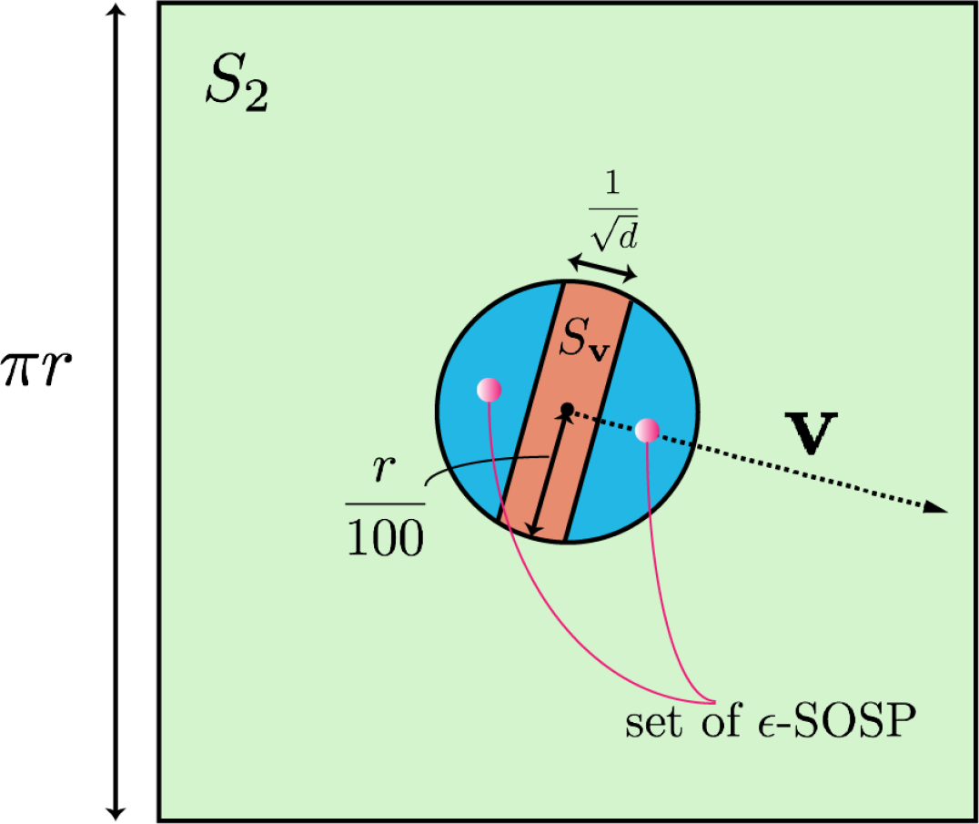
Figure 4: Key regions in lower bound

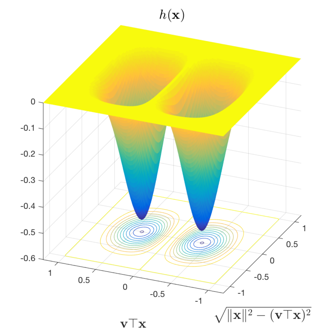
Figure 5: Landscape of $h$

Constructing a lower-bound example within a ball

The target function $F(\mathbf{x})$ we construct contains a special direction $\mathbf{v}$ in a $d$-dimensional ball $\mathbb{B}_{r}$ with radius $r$ centered at the origin. More concretely, let $F(\mathbf{x})=h(\mathbf{x})+\|{\mathbf{x}}\|^{2}$, where $h$ (see Figure 5) depends on a special direction $\mathbf{v}$, but is spherically symmetric in its orthogonal subspace. Let the direction $\mathbf{v}$ be sampled uniformly at random from the $d$-dimensional unit sphere. Define a region around the equator of $\mathbb{B}_{r}$, denoted $S_{\mathbf{v}}=\{\mathbf{x}|\mathbf{x}\in\mathbb{B}_{r}\text{~{}and~{}}|\mathbf{v}^{\top}\mathbf{x}|\leq r\log d/\sqrt{d}\}$, as in Figure 5. The key ideas of this construction relying on the following three properties:

1. For any fixed point $\mathbf{x}$ in $\mathbb{B}_{r}$, we have $\Pr(\mathbf{x}\in S_{\mathbf{v}})\geq 1-O(1/d^{\log d})$.

2. The $\epsilon$-SOSP of $F$ is located in a very small set $\mathbb{B}_{r}-S_{\mathbf{v}}$.

3. $h(\mathbf{x})$ has very small function value inside $S_{\mathbf{v}}$, that is, $\sup_{\mathbf{x}\in S_{\mathbf{v}}}|h(\mathbf{x})|\leq\tilde{O}(1/d)$.

The first property is due to the concentration of measure in high dimensions. The latter two properties are intuitively shown in Figure 5. These properties suggest a natural construction for $f$:

$$f(\mathbf{x})=\begin{cases}\|{\mathbf{x}}\|^{2}&\qquad\text{~{}if~{}}\mathbf{x}\in S_{\mathbf{v}}\\ F(\mathbf{x})&\qquad\text{~{}otherwise~{}}\end{cases}.$$

When $\mathbf{x}\in S_{\mathbf{v}}$, by property 3 above we know $|f(\mathbf{x})-F(\mathbf{x})|\leq\nu=\tilde{O}(1/d)$.

To see why this construction gives a hard instance of Problem 1, recall that the direction $\mathbf{v}$ is uniformly random. Since the direction $\mathbf{v}$ is unknown to the algorithm at initialization, the algorithm’s first query is independent of $\mathbf{v}$ and thus is likely to be in region $S_{\mathbf{v}}$, due to property 1. The queries inside $S_{\mathbf{v}}$ give no information about $\mathbf{v}$, so any polynomial-time algorithm is likely to continue to make queries in $S_{\mathbf{v}}$ and eventually fail to find $\mathbf{v}$. On the other hand, by property 2 above, finding an $\epsilon$-SOSP of $F$ requires approximately identifying the direction of $\mathbf{v}$, so any polynomial-time algorithm will fail with high probability.

Extending to the entire space

To extend this construction to the entire space $\mathbb{R}^{d}$, we put the ball (the previous construction) inside a hypercube (see Figure 5) and use the hypercube to tile the entire space $\mathbb{R}^{d}$. There are two challenges in this approach: (1) The function $F$ must be smooth even at the boundaries between hypercubes; (2) The padding region ($S_{2}$ in Figure 5) between the ball and the hypercube must be carefully constructed to not ruin the properties of the hard functions.

We deal with first problem by constructing a function $\bar{F}(\mathbf{y})$ on $[-1,1]^{d}$, ignoring the boundary condition, and then composing it with a smooth periodic function. For the second problem, we carefully construct a smooth function $h$, as shown in Figure 5, to have zero function value, gradient and Hessian at the boundary of the ball and outside the ball, so that no algorithm can make use of the padding region to identify an SOSP of $F$. Details are deferred to section C in the appendix.

Appendix C Constructing Hard Functions

In this section, we prove Theorem 8, the lower bound for algorithms making a polynomial number of queries. We start by describing the hard function construction that is key to the lower bound.

C.1 “Scale-free” hard instance

We will first present a “scale-free” version of the hard function, where we assume $\rho=1$ and $\epsilon=1$. In section C.2, we will show how to scale this hard function to prove Theorem 8.

Denote $\sin\mathbf{x}=(\sin(x_{1}),\cdots,\sin(x_{d}))$. Let $\mathbb{I}\{a\}$ denote the indicator function that takes value $1$ when event $a$ happens and $0$ otherwise. Let $\mu=300$ . Let the function $F:\mathbb{R}^{d}\to\mathbb{R}$ be defined as follows.

$$F(\mathbf{x})=h(\sin\mathbf{x})+\|{\sin\mathbf{x}}\|^{2},$$ (7)

where $h(\mathbf{y})=h_{1}(\mathbf{v}^{\top}\mathbf{y})\cdot h_{2}(\sqrt{\|{\mathbf{y}}\|^{2}-(\mathbf{v}^{\top}\mathbf{y})^{2}})$, and

$$h_{1}(x) =g_{1}(\mu x),\quad g_{1}(x)=\left(-16|x|^{5}+48x^{4}-48|x|^{3}+16x^{2}\right)\mathbb{I}\{|x|<1\},$$

$$h_{2}(x) =g_{2}(\mu x),\quad g_{2}(x)=\left(3x^{4}-8|x|^{3}+6x^{2}-1\right)\mathbb{I}\{|x|<1\},$$

and the vector $\mathbf{v}$ is uniformly distributed on the $d$-dimensional unit sphere.

Figure 6: Polynomials $g_{1},g_{2}$

We will state the properties of the hard instance by breaking the space into different regions:

• “ball” $S=\{\mathbf{x}\in\mathbb{R}^{d}:\|{\mathbf{x}}\|\leq 3/\mu\}$ be the $d$-dimensional ball with radius $3/\mu$.

• “hypercube” $H=[-\frac{\pi}{2},\frac{\pi}{2}]^{d}$ be the $d$-dimensional hypercube with side length $\pi$.

• “band” $S_{\mathbf{v}}=\{\mathbf{x}\in S:\langle\sin\mathbf{x},\mathbf{v}\rangle\leq\frac{\log d}{\sqrt{d}}\}$

• “padding” $S_{2}=H-S$

We also call the union of $S_{2}$ and $S_{\mathbf{v}}$ the “non-informative” region.

Define the perturbed function, $f$:

$$f(\mathbf{x})=\begin{cases}\|{\sin\mathbf{x}}\|^{2},&\mathbf{x}\in S_{\mathbf{v}}\\ F(\mathbf{x}),&\mathbf{x}\notin S_{\mathbf{v}}.\end{cases}$$ (8)

Our construction happens within the ball. However it is hard to fill the space using balls, so we pad the ball into a hypercube. Our construction will guarantee that any queries to the non-informative region do not reveal any information about $\mathbf{v}$. Intuitively the non-informative region is very large so that it is hard for the algorithm to find any point outside of the non-informative region (and learn any information about $\mathbf{v}$).

Lemma 33 (Properties of scale-free hard function pair $F,f$).

Let $F,f,\mathbf{v}$ be as defined in equations (7), (8). Then $F,f$ satisfies:

1. $f$ in the non-informative region $S_{2}\cup S_{\mathbf{v}}$ is independent of $\mathbf{v}$.

2. $\sup_{x\in S_{\mathbf{v}}}|f-F|\leq\tilde{O}(\frac{1}{d})$.

3. $F$ has no SOSP in the non-informative region $S_{2}\cup S_{\mathbf{v}}$.

4. $F$ is $O(d)$-bounded, $O(1)$-Hessian Lipschitz, and $O(1)$-gradient Lipschitz.

These properties will be proved based on the properties of $h(\mathbf{y})$, which we defined in (7) to be the product of two functions.

Proof.

Property 1. On $S_{\mathbf{v}}$, $f(\mathbf{x})=F(\mathbf{x})=\|{\sin\mathbf{x}}\|^{2}$, which is independent of $\mathbf{v}$. On $S_{2}$, we argue that $h(\sin\mathbf{x})=0$ and therefore $f(\mathbf{x})=\|{\sin\mathbf{x}}\|^{2}~{}\forall\mathbf{x}\in S_{2}$. Note that on $S_{2}$, $\|{\mathbf{x}}\|>3/\mu$ and $(\sin x)^{2}>(\frac{2x}{\pi})^{2}~{}\forall|x|<\frac{\pi}{2}$, so

$$\|{\sin\mathbf{x}}\|>\|{\frac{2\mathbf{x}}{\pi}}\|>\frac{6}{\pi\mu}\implies\max\left\{\mathbf{v}^{\top}\sin\mathbf{x},\sqrt{\|{\sin\mathbf{x}}\|^{2}-(\mathbf{v}^{\top}\sin\mathbf{x})^{2}}\right\}>\frac{6}{\sqrt{2}\cdot\pi\mu}>\frac{1}{\mu}.$$

Therefore, $h(\sin\mathbf{x})=h_{1}(\mathbf{v}^{\top}\sin\mathbf{x})\cdot h_{2}(\sqrt{\|{\sin\mathbf{x}}\|^{2}-(\mathbf{v}^{\top}\sin\mathbf{x})^{2}})=0$.

Property 2. It suffices to show that for $\mathbf{x}\in S_{\mathbf{v}}$, $|h(\sin\mathbf{x})|=\tilde{O}(\frac{1}{d})$.

For $\mathbf{x}\in S_{\mathbf{v}}$, we have $\mathbf{v}^{\top}\sin\mathbf{x}\in[-\frac{\log d}{\sqrt{d}},\frac{\log d}{\sqrt{d}}]$. By symmetry, we may just consider the case where $\mathbf{v}^{\top}\sin\mathbf{x}>0$.

$$|h(\sin\mathbf{x})| \leq|h_{1}(\mathbf{v}^{\top}\sin\mathbf{x})|$$

$$=|\left(-16|x|^{5}+48x^{4}-48|x|^{3}+16x^{2}\right)|\text{ where $x=\mu\mathbf{v}^{\top}\sin\mathbf{x}$}$$

$$\leq C(\frac{\log d}{\sqrt{d}})^{2}$$

$$\leq C\frac{\log^{2}d}{d}$$

Here $C>0$ is a large enough universal constant.

Property 3. (Part I.) We show that there are no SOSP in $S_{2}$. For $\mathbf{x}:\|{\mathbf{x}}\|>3/\mu$, we argue that either the gradient is large, due to contribution from $\|{\sin\mathbf{x}}\|^{2}$, or the Hessian has large negative eigenvalue (points close to the boundary of $H$). Denote $G(\mathbf{x})=\|{\sin\mathbf{x}}\|^{2}$. We may compute the gradient of $G$ as follows:

$$\frac{\partial}{\partial x_{i}}G(\mathbf{x}) =2\sin(x_{i})\cos(x_{i})=\sin(2x_{i}),$$

$$\|{\nabla G(\mathbf{x})}\| =\sqrt{\sum_{i}(\sin(2x_{i}))^{2}}\geq\sqrt{\sum_{i}x_{i}^{2}}=\|{\mathbf{x}}\|\text{ for all $\mathbf{x}\in[-\xi,\xi]^{d}$},$$

where $\xi\approx 0.95$ is the positive root of the equation $\sin 2x=x$. On $S_{2}$, $\nabla F(\mathbf{x})=\nabla G(\mathbf{x})$, so $\|{\nabla F(\mathbf{x})}\|>\frac{3}{\mu}=1\times 10^{-2}$ for $\mathbf{x}\in S_{2}\cap[-\xi,\xi]^{d}$. We may also compute the Hessian of $G$:

$$\nabla^{2}G(\mathbf{x}) =diag(2\cos(2\mathbf{x})),$$

$$\lambda_{\min}(\nabla^{2}G(\mathbf{x})) =\min_{i}\{2\cos(2x_{i})\}\leq 2\cdot(\frac{\pi}{4}-x)<2\cdot(\frac{\pi}{4}-\xi)~{}\forall\mathbf{x}\in S_{2}\setminus[-\xi,\xi]^{d}.$$

Since $(\frac{\pi}{4}-\xi)<-0.15$, $\lambda_{\min}(\nabla^{2}F(\mathbf{x}))<-0.3$.

(Part II.) We argue that $F$ has no SOSP in $S_{\mathbf{v}}$. For $\mathbf{y}=\sin(\mathbf{x})$, we consider two cases: (i) $z=\sqrt{\|{\mathbf{y}}\|^{2}-(\mathbf{v}^{\top}\mathbf{y})^{2}}$ large and (ii) $z$ small.

Write $g(\mathbf{x})=h(\sin\mathbf{x})$, and denote $\left.\nabla h(\mathbf{x})\right|_{\sin\mathbf{x}},\left.\nabla^{2}h(\mathbf{x})\right|_{\sin\mathbf{x}}$ with $\nabla h(\mathbf{y}),\nabla^{2}h(\mathbf{y})$. Let $\mathbf{u}\circ\mathbf{v}$ denote the Schur product of $\mathbf{u}$ and $\mathbf{v}$. We may compute the gradient and Hessian of $g$:

$$\nabla g(\mathbf{x})=\nabla h(\mathbf{y})\circ\cos(\mathbf{x}),$$

$$\nabla^{2}g(\mathbf{x})=diag(\cos\mathbf{x}))\nabla^{2}h(\mathbf{y})diag(\cos\mathbf{x}))-\nabla h(\mathbf{y})\circ\sin(\mathbf{x}).$$

Now we change the coordinate system such that $\mathbf{v}=(1,0,\cdots,0)$. $\|{\nabla h(\mathbf{y})}\|$ and $\lambda_{\min}(\nabla^{2}h(\mathbf{y}))$ are invariant to such a transform. Under this coordinate system, $h(\mathbf{y})=h_{1}(y_{1})\cdot h_{2}(\sqrt{\|{\mathbf{y}}\|^{2}-(y_{1})^{2}})$

(i): $z\geq\frac{1}{2\mu}$. We show that $\|{\nabla F}\|$ is large.

Let $\mathcal{P}_{-1}(\mathbf{u})$ denote the projection of $\mathbf{u}$ onto the orthogonal component of the first standard basis vector.

Since $\forall~{}i\neq 1,\frac{\partial}{\partial y_{i}}h(\mathbf{y})=h_{1}(y_{1})h_{2}^{\prime}(z)\frac{y_{i}}{z}$, we have

$$\mathcal{P}_{-1}(\nabla h(\mathbf{y})) =\frac{h_{1}(y_{1})h_{2}^{\prime}(z)}{z}\mathcal{P}_{-1}(\mathbf{y})\text{ where }\frac{h_{1}(y_{1})h_{2}^{\prime}(z)}{z}>0$$

$$\mathcal{P}_{-1}(\nabla F(\mathbf{x})) =\mathcal{P}_{-1}(\nabla g(\mathbf{x})+\nabla G(x))=\mathcal{P}_{-1}(\nabla h(\mathbf{y})\circ\cos(\mathbf{x})+\mathbf{y}\circ\cos\mathbf{x})$$

$$=\left(\frac{h_{1}(y_{1})h_{2}^{\prime}(z)}{z}\mathcal{P}_{-1}(\mathbf{y})+\mathcal{P}_{-1}(\mathbf{y})\right)\circ\cos\mathbf{x}$$

$$\|{\nabla F(\mathbf{x}))}\| \geq\|{\mathcal{P}_{-1}(\nabla F(\mathbf{x}))}\|\geq\|{\mathcal{P}_{-1}(\mathbf{y})\circ\cos\mathbf{x}}\|\geq z\cdot\min_{i}|\cos(x_{i})|$$

$$\geq\frac{1}{2\mu}\cdot 0.999\geq 1\times 10^{-3}~{}\text{ since $|x_{i}|\leq 3/\mu$ }$$

(ii): $z<\frac{1}{2\mu}$. We show that $\nabla^{2}F(\mathbf{x})$ has large negative eigenvalue. First we compute the second derivative of $h$ in the direction of the first coordinate:

$$\frac{\partial^{2}h}{\partial y_{1}^{2}}=h_{2}(z)h_{1}^{\prime\prime}(y_{1})\leq 32\mu^{2}g_{2}(1/2)=-10\mu^{2}.$$

Now we use this to upper bound the smallest eigenvalue of $\nabla^{2}F(\mathbf{x})$.

$$\lambda_{\min}(\nabla^{2}h(\mathbf{y})) \leq\min_{i}\frac{\partial^{2}}{\partial y_{i}^{2}}h(\mathbf{y})\leq\frac{\partial^{2}h}{\partial y_{1}^{2}}$$

$$\lambda_{\min}(\nabla^{2}g(\mathbf{x})) \leq\left(\lambda_{\min}\left(diag(\cos\mathbf{x})\nabla^{2}h(\mathbf{y})diag(\cos\mathbf{x})\right)+\lambda_{\max}\left(-diag(\nabla h(\mathbf{y})\circ\sin(\mathbf{x}))\right)\right)$$

$$\leq-0.999\cdot 10\mu^{2}+0.01\cdot\max_{\mathbf{y}}(h_{2}(z)h_{1}^{\prime}(y_{1})+h_{1}(y_{1})h_{2}^{\prime}(z))~{}\text{ since $|x_{i}|\leq 3/\mu$}$$

$$\leq-0.999\cdot 10\mu^{2}+0.01\cdot 3\mu$$

Finally,

$$\nabla^{2}G(\mathbf{x}) =diag(2\cos(2\mathbf{x}))\implies\|{\nabla^{2}G(\mathbf{x})}\|\leq 2,$$

$$\lambda_{\min}(\nabla^{2}F(\mathbf{x})) \leq-0.999\cdot 10\mu^{2}+0.01\cdot 3\mu+2\leq-8\times 10^{5}.$$

Property 4. $O(1)$-bounded: Lemma 34 shows that $|h(\mathbf{y})|\leq 1$. $\|{\sin\mathbf{x}}\|^{2}\leq d$. Therefore $|F|\leq 1+d$.

$O(1)$-gradient Lipschitz: $\|{\nabla^{2}F(\mathbf{x})}\|\leq\|{\nabla^{2}G(\mathbf{x})}\|+\|{\nabla^{2}g(\mathbf{x})}\|$. We know $\|{\nabla^{2}G(\mathbf{x})}\|\leq 2$.

$$\|{\nabla^{2}g(\mathbf{x})}\| =\|{diag(\cos\mathbf{x})\nabla^{2}h(\mathbf{y})diag(\cos\mathbf{x})-diag(\nabla h(\mathbf{y})\circ\sin(\mathbf{x}))}\|$$

$$\leq\|{diag(\cos\mathbf{x})}\|^{2}\cdot\|{\nabla^{2}h(\mathbf{y})}\|+\|{diag(\nabla h(\mathbf{y}))}\|\cdot\|{diag(\sin\mathbf{x})}\|$$

$$\leq 1\cdot 68\mu^{2}+3\mu\cdot 1\leq 7\times 10^{6}~{}\text{ using lemma \ref{lemma:h_function} }$$

$O(1)$-Hessian Lipschitz: First bound the Hessian Lipschitz constant of $G(\mathbf{x})$.

$$\|{\nabla^{2}G(\mathbf{x})-\nabla^{2}G(\mathbf{z})}\|\leq 2\|{\cos(2\mathbf{x})-\cos(2\mathbf{z})}\|\leq 4\|{\mathbf{x}-\mathbf{z}}\|.$$

Now we bound the Hessian Lipschitz constant of $g(\mathbf{x})$. Denote $\mathbf{A}(\mathbf{x})=diag(\cos\mathbf{x})$ and $\mathbf{B}(\mathbf{x})=diag(\sin\mathbf{x})$.

$$\|{\mathbf{A}(\mathbf{x}_{1})\nabla^{2}h(\mathbf{y}_{1})\mathbf{A}(\mathbf{x}_{1})-\mathbf{A}(\mathbf{x}_{2})\nabla^{2}h(\mathbf{y}_{2})\mathbf{A}(\mathbf{x}_{2})}\|$$

$$\leq \|\mathbf{A}(\mathbf{x}_{1})\nabla^{2}h(\mathbf{y}_{1})\mathbf{A}(\mathbf{x}_{1})-\mathbf{A}(\mathbf{x}_{1})\nabla^{2}h(\mathbf{y}_{1})\mathbf{A}(\mathbf{x}_{2})\|+\|\mathbf{A}(\mathbf{x}_{1})\nabla^{2}h(\mathbf{y}_{1})\mathbf{A}(\mathbf{x}_{2})-\mathbf{A}(\mathbf{x}_{1})\nabla^{2}h(\mathbf{y}_{2})\mathbf{A}(\mathbf{x}_{2})\|$$

$$+\mathbf{A}(\mathbf{x}_{1})\nabla^{2}h(\mathbf{y}_{2})\mathbf{A}(\mathbf{x}_{2})-\mathbf{A}(\mathbf{x}_{2})\nabla^{2}h(\mathbf{y}_{2})\mathbf{A}(\mathbf{x}_{2})\|$$

$$\leq 68\mu^{2}\|{\mathbf{x}_{1}-\mathbf{x}_{2}}\|+1000\mu^{3}\|{\mathbf{x}_{1}-\mathbf{x}_{2}}\|+68\mu^{2}\|{\mathbf{x}_{1}-\mathbf{x}_{2}}\|\text{ from lemma \ref{lemma:h_function}}.$$

$$\|{diag(\nabla h(\mathbf{y}_{1}))\mathbf{B}(\mathbf{x}_{1})-diag(\nabla h(\mathbf{y}_{2}))\mathbf{B}(\mathbf{x}_{2})}\|$$

$$\leq \|{diag(\nabla h(\mathbf{y}_{1}))\mathbf{B}(\mathbf{x}_{1})-diag(\nabla h(\mathbf{y}_{1}))\mathbf{B}(\mathbf{x}_{2})}\|+\|{diag(\nabla h(\mathbf{y}_{1}))\mathbf{B}(\mathbf{x}_{2})-diag(\nabla h(\mathbf{y}_{2}))\mathbf{B}(\mathbf{x}_{2})}\|$$

$$\leq (3\mu+68\mu^{2})\|{\mathbf{x}_{1}-\mathbf{x}_{2}}\|\text{ from lemma \ref{lemma:h_function}}.$$

$$\|{\nabla^{2}g(\mathbf{x}_{1})-\nabla^{2}g(\mathbf{x}_{2})}\|$$

$$= (144\mu^{3}+204\mu^{2}+3\mu)\|{\mathbf{x}_{1}-\mathbf{x}_{2}}\|.$$

Therefore $F(\mathbf{x})$ is $(2.8\times 10^{10})$-Hessian Lipschitz.

∎

Now we need to prove smoothness properties of $h(\mathbf{y})$ that are used in the previous proof. In the following lemma, we prove that $h(\mathbf{y})$ as defined in equation (7) is bounded, Lipschitz, gradient-Lipschitz, and Hessian-Lipschitz.

Lemma 34 (Properties of $h(\mathbf{y})$).

$h(\mathbf{y})$ as given in Definition 7 is O(1)-bounded, O(1)-Lipschitz, O(1)-gradient Lipschitz, and O(1)-Hessian Lipschitz.

Proof.

WLOG assume $\mathbf{v}=(1,0,\cdots,0)^{\top}$. Denote $u=y_{1},\mathbf{w}=(y_{2},\cdots,y_{d})^{\top}$. Let $\otimes$ denote tensor product.

Note that $|h_{1}^{\prime}|\leq 3\mu,|h_{2}^{\prime}|\leq 2\mu,|h_{1}^{\prime\prime}|\leq 32\mu^{2},|h_{2}^{\prime\prime}|\leq 12\mu^{2},|h_{1}^{\prime\prime\prime}|\leq 300\mu^{3},|h_{2}^{\prime\prime\prime}|\leq 48\mu^{3}$. Assume $\mu>2$.

1. O(1)-bounded: $|h|\leq|h_{1}|\cdot|h_{2}|\leq 1$.

2. O(1)-Lipschitz: $\|{\nabla h(\mathbf{y})}\|=\sqrt{h_{2}(\|{\mathbf{w}}\|)h_{1}^{\prime}(u)+h_{1}(u)h_{2}^{\prime}(\|{\mathbf{w}}\|)}\leq 3\mu\leq O(1)$.

3. O(1)-gradient Lipschitz:

   $$\nabla^{2}h(\mathbf{y})=h_{1}(u)\nabla^{2}h_{2}(\|{\mathbf{w}}\|)+h_{2}(\|{\mathbf{w}}\|)\nabla^{2}h_{1}(u)+\nabla h_{1}(u)\nabla h_{2}(\|{\mathbf{w}}\|)^{\top}+\nabla h_{2}(\|{\mathbf{w}}\|)\nabla h_{1}(u)^{\top}.$$

   $\|{\nabla h_{1}(u)}\|\leq 3\mu$. Notice that the following are also O(1):

   $$\|{\nabla h_{2}(\|{\mathbf{w}}\|)}\|=\|{h_{2}^{\prime}(\|{\mathbf{w}}\|)\frac{\mathbf{w}}{\|{\mathbf{w}}\|}}\|\leq 2\mu;$$

   $$\|{\nabla^{2}h_{2}(\mathbf{w})}\|\leq\|{h_{2}^{\prime\prime}(\|{\mathbf{w}}\|)\frac{\mathbf{w}\mathbf{w}^{\top}}{\|{\mathbf{w}}\|^{2}}}\|+\|{h_{2}^{\prime}(\|{\mathbf{w}}\|)\frac{\|{\mathbf{w}}\|^{2}\mathbf{I}-\mathbf{w}\mathbf{w}^{\top}}{\|{\mathbf{w}}\|^{3}}}\|\leq|h_{2}^{\prime\prime}(\|{\mathbf{w}}\|)|+|h_{2}^{\prime}(\|{\mathbf{w}}\|)/\|{\mathbf{w}}\||\leq 12\mu^{2}+12\mu.$$

   Therefore, $\|{\nabla^{2}h(\mathbf{y})}\|\leq 24\mu^{2}+32\mu^{2}+2\cdot 2\mu\cdot 3\mu\leq 68\mu^{2}$.

4. O(1)-Hessian Lipschitz: We first argue that $\nabla^{2}h_{2}(\mathbf{w})$ is Lipschitz. For $\|{\mathbf{w}}\|\geq 1/\mu$, $\nabla^{2}h_{2}(\mathbf{w})=0$. So we consider $\|{\mathbf{w}}\|<\mu$. We obtain the following by direct computation.

   $$\nabla^{2}h_{2}(\mathbf{w}) =h_{2}^{\prime\prime}(\|{\mathbf{w}}\|)\frac{\mathbf{w}\mathbf{w}^{\top}}{\|{\mathbf{w}}\|^{2}}+h_{2}^{\prime}(\|{\mathbf{w}}\|)\frac{\|{\mathbf{w}}\|^{2}\mathbf{I}-\mathbf{w}\mathbf{w}^{\top}}{\|{\mathbf{w}}\|^{3}}$$

   $$=24\mu^{4}\mathbf{w}\mathbf{w}^{\top}-24\mu^{3}\frac{\mathbf{w}\mathbf{w}^{\top}}{\|{\mathbf{w}}\|}+(12\mu^{4}\|{\mathbf{w}}\|^{2}-24\mu^{3}\|{\mathbf{w}}\|+12\mu^{2})\mathbf{I}$$

   $$\nabla^{3}h_{2}(\mathbf{w}) =24\mu^{4}(\mathbf{w}\otimes\mathbf{I}+\mathbf{I}\otimes\mathbf{w})-24\mu^{3}\frac{\|{\mathbf{w}}\|^{2}(\mathbf{w}\otimes\mathbf{I}+\mathbf{I}\otimes\mathbf{w})-\mathbf{w}\otimes\mathbf{w}\otimes\mathbf{w}}{\|{\mathbf{w}}\|^{3}}$$

   $$+24\mu^{4}\mathbf{I}\otimes\mathbf{w}-24\mu^{3}\frac{\mathbf{I}\otimes\mathbf{w}}{\|{\mathbf{w}}\|}$$

   $$\|{\nabla^{3}h_{2}(\mathbf{w})}\| \leq 48\mu^{3}+72\mu^{2}+24\mu^{3}+24\mu^{2}\leq 144\mu^{3}$$

   We may easily check that indeed $\lim_{\|{\mathbf{w}}\|\to 1}\|{\nabla^{2}h_{2}(\mathbf{w})}\|=0$.

   Therefore $\nabla^{2}h_{2}(\mathbf{w})$ is $144\mu^{3}$-Lipschitz.

   $$\|{h_{1}(u_{1})\nabla^{2}h_{2}(\|{\mathbf{w}_{1}}\|)-h_{1}(u_{2})\nabla^{2}h_{2}(\|{\mathbf{w}_{1}}\|)}\| \leq(144\mu^{3}+3\mu\cdot 24\mu^{2})\|{\mathbf{y}_{1}-\mathbf{y}_{2}}\|$$

   $$\|{h_{2}(\|{\mathbf{w}_{1}}\|)\nabla^{2}h_{1}(u_{1})-h_{2}(\|{\mathbf{w}_{2}}\|)\nabla^{2}h_{1}(u_{2})}\| \leq(32\mu^{2}\cdot 2\mu+300\mu^{3})\|{\mathbf{y}_{1}-\mathbf{y}_{2}}\|$$

   $$\|{\nabla h_{1}(u_{1})\nabla h_{2}(\|{\mathbf{w}_{1}}\|)^{\top}-\nabla h_{1}(u_{2})\nabla h_{2}(\|{\mathbf{w}_{2}}\|)^{\top}}\| \leq(3\mu\cdot 24\mu^{2}+2\mu\cdot 32\mu^{2})\|{\mathbf{y}_{1}-\mathbf{y}_{2}}\|$$

   By triangle inequality, using the above, we obtain

   $$\|{\nabla^{2}h(\mathbf{y}_{1})-\nabla^{2}h(\mathbf{y}_{2})}\|\leq 1000\mu^{3}\|{\mathbf{y}_{1}-\mathbf{y}_{2}}\|.$$

   This proves that $h(\mathbf{y})$ is $1000\mu^{3}$-Hessian Lipschitz.

∎

C.2 Scaling the Hard Instance

Now we show how to scale the function we described in order to achieve the final lower bound with correct dependencies on $\epsilon$ and $\rho$.

Given any $\epsilon,\rho>0$, define

$$\tilde{F}(\mathbf{x})=\epsilon rF(\frac{1}{r}\mathbf{x}),\tilde{f}(\mathbf{x})=\epsilon rf(\frac{1}{r}\mathbf{x}),$$ (9)

where $r=\sqrt{\epsilon/\rho}$ and $F,f$ are defined as in Equation 7. Define the ‘scaled’ regions:

• $\tilde{S}=\{\mathbf{x}\in\mathbb{R}^{d}:\|{\mathbf{x}}\|\leq 3r/\mu\}$ be the $d$-dimensional ball with radius $3r/\mu$.

• $\tilde{H}=[-\frac{\pi}{2}r,\frac{\pi}{2}r]^{d}$ be the $d$-dimensional hypercube with side length $\pi r$.

• $\tilde{S}_{\mathbf{v}}=\{\mathbf{x}\in\tilde{S}:\langle\sin\frac{1}{r}\mathbf{x},\mathbf{v}\rangle\leq\frac{\log d}{\sqrt{d}}\}$.

• $\tilde{S}_{2}=\tilde{H}-\tilde{S}$.

Defined as above, $(\tilde{F},\tilde{f})$ satisfies the properties stated in lemma 35, which makes it hard for any algorithm to optimize $\tilde{F}$ given only access to $\tilde{f}$.

Lemma 35.

Let $\tilde{F},\tilde{f},\mathbf{v},\tilde{S}_{2},\tilde{S}_{\mathbf{v}}$ be as defined in 9. Then for any $\epsilon,\rho>0$, $F,f$ satisfies:

1. $\tilde{f}$ in the non-informative region $\tilde{S}_{2}\cup\tilde{S}_{\mathbf{v}}$ is independent of $\mathbf{v}$.

2. $\sup_{x\in\tilde{S}_{\mathbf{v}}}|\tilde{f}-\tilde{F}|\leq\frac{\epsilon^{1.5}}{\sqrt{\rho}d}$ up to poly-$\log{d}$ and constant factors.

3. $\tilde{F}$ has no $O(\epsilon)$-SOSP in the non-informative region $\tilde{S}_{2}\cup\tilde{S}_{\mathbf{v}}$.

4. $\tilde{F}$ is $B$-bounded, $O(\rho)$-Hessian Lipschitz, and $O(\ell)$-gradient Lipschitz.

Proof.

This is implied by Lemma 33. To see this, notice

1. We have simply scaled each coordinate axis by $r$.

2. $|\tilde{F}-\tilde{f}|=\epsilon r|F-f|=\frac{\epsilon^{1.5}}{\sqrt{\rho}}|F-f|$.

3. $\|{\nabla\tilde{F}}\|=\epsilon\|{\nabla F}\|$ and $\|{\nabla^{2}\tilde{F}}\|=\sqrt{\rho\epsilon}\|{\nabla^{2}F}\|$. Since $F$ has no $1\times 10^{-12}$-SOSP in $S_{2}\cup S_{\mathbf{v}}$. Taking into account the Hessian Lipschitz constant of $F$, $\tilde{F}$ has no $\frac{\epsilon}{10^{12}}$-SOSP in $\tilde{S}_{2}\cup\tilde{S}_{\mathbf{v}}$.

4. We must have $B>d+\frac{\epsilon^{1.5}}{\sqrt{\rho}}$. Then, $\tilde{F}$ is $B$-bounded, $(7\times 10^{6})\sqrt{\rho\epsilon}$- gradient Lipschitz, and $(2.8\times 10^{10})\rho$-Hessian Lipschitz.

∎

C.3 Proof of the Theorem

We are now ready to state the two main lemmas used to prove Theorem 8.

The following lemma uses the concentration of measure in higher dimensions to argue that the probability that any fixed point lies in the informative region $\tilde{S}_{\mathbf{v}}$ is very small.

Lemma 36 (Probability of landing in informative region).

For any arbitrarily fixed point $\mathbf{x}\in\tilde{S}$, $\Pr(\mathbf{x}\notin\tilde{S}_{\mathbf{v}})\leq 2e^{-(\log d)^{2}/2}$.

Proof.

Recall the definition of $\tilde{S}_{\mathbf{v}}$: $\tilde{S}_{\mathbf{v}}=\{\mathbf{x}\in\tilde{S}:\langle\sin\frac{1}{r}\mathbf{x},\mathbf{v}\rangle\leq\frac{\log d}{\sqrt{d}}\}$. Since $\mathbf{x}\in\tilde{S}$, we have $\|{\mathbf{x}}\|\leq 3r/\mu\leq r$ (as $\mu\geq 3$). Therefore, by inequality $|\sin\theta|\leq|\theta|$, we have:

$$\|{\sin\frac{\mathbf{x}}{r}}\|^{2}=\sum_{i=1}^{d}|\sin\frac{x^{(i)}}{r}|^{2}\leq\sum_{i=1}^{d}|\frac{x^{(i)}}{r}|^{2}\leq 1.$$

Denote unit vector $\hat{\mathbf{y}}=\sin\frac{\mathbf{x}}{r}/\|{\sin\frac{\mathbf{x}}{r}}\|$. This gives:

$$\Pr(\mathbf{x}\notin\tilde{S}_{\mathbf{v}}) =\Pr(|\langle\sin\frac{\mathbf{x}}{r},\mathbf{v}\rangle|\geq\frac{\log d}{\sqrt{d}})=\Pr(|\langle\hat{\mathbf{y}},\mathbf{v}\rangle|\geq\frac{\log d}{\sqrt{d}\|{\sin\frac{\mathbf{x}}{r}}\|})$$

$$\leq\Pr(|\langle\hat{\mathbf{y}},\mathbf{v}\rangle|\geq\frac{\log d}{\sqrt{d}})\text{ ~{}~{}since~{}}\|{\sin\frac{\mathbf{x}}{r}}\|\leq 1$$

$$=\frac{\text{Area}(\{\mathbf{u}:\|{\mathbf{u}}\|=1,|\langle\hat{\mathbf{y}},\mathbf{u}\rangle|>\frac{\log d}{\sqrt{d}}\})}{\text{Area}(\{\mathbf{u}:\|{\mathbf{u}}\|=1\})}$$

$$\leq 2e^{-(\log d)^{2}/2}\text{ by lemma }\ref{lemma_sa_conc_sphere}$$

This finishes the proof. ∎

Thus we know that for a single fixed point, the probability of landing in $\tilde{S}_{\mathbf{v}}$ is less than $2(1/d)^{\log d/2}$. We note that this is smaller than $1/\text{poly}(d)$. The following lemma argues that even for a possibly adaptive sequence of points (of polynomial size), the probability that any of them lands in $\tilde{S}_{\mathbf{v}}$ remains small, as long as the query at each point does not reveal information about $\tilde{S}_{\mathbf{v}}$.

Lemma 37 (Probability of adaptive sequences landing in the informative region).

Consider a sequence of points and corresponding queries with size $T$: $\{(\mathbf{x}_{i},q(\mathbf{x}_{i}))\}_{i=1}^{T}$, where the sequence can be adaptive, i.e. $\mathbf{x}_{t}$ can depend on all previous history $\{(\mathbf{x}_{i},q(\mathbf{x}_{i}))\}_{i=1}^{t-1}$. Then as long as $q(\mathbf{x}_{i})\perp\mathbf{v}~{}|~{}\mathbf{x}_{i}\in\tilde{S}_{\mathbf{v}}$, we have $\Pr(\exists t\leq T:\mathbf{x}_{t}\not\in\tilde{S}_{\mathbf{v}})\leq 2Te^{-(\log d)^{2}/2}$.

Proof.

Clearly $\Pr(\exists t\leq T:\mathbf{x}_{t}\not\in\tilde{S}_{\mathbf{v}})=1-\Pr(\forall t\leq T:\mathbf{x}_{t}\in\tilde{S}_{\mathbf{v}})$. By product rule, we have:

$$\Pr(\forall t\leq T:\mathbf{x}_{t}\in\tilde{S}_{\mathbf{v}})=\prod_{t=1}^{T}\Pr(\mathbf{x}_{t}\in\tilde{S}_{\mathbf{v}}|\forall\tau<t:\mathbf{x}_{\tau}\in\tilde{S}_{\mathbf{v}}).$$

Denote $D_{i}=\{\mathbf{v}\in\mathbb{S}^{d-1}|\langle\sin\frac{1}{r}\mathbf{x}_{i},\mathbf{v}\rangle>\frac{\log d}{\sqrt{d}}\}$, where $\mathbb{S}^{d-1}$ denotes the unit sphere in $\mathbb{R}^{d}$ centered at the origin. Clearly, $\mathbf{v}\not\in D_{i}$ is equivalent to $\mathbf{x}_{i}\in\tilde{S}_{\mathbf{v}}$. Consider term $\Pr(\mathbf{x}_{t}\in\tilde{S}_{\mathbf{v}}|\forall\tau<t:\mathbf{x}_{\tau}\in\tilde{S}_{\mathbf{v}})$. Conditioned on the event that $E=\{\forall\tau<t:\mathbf{x}_{\tau}\in\tilde{S}_{\mathbf{v}}\}$, we know $\mathbf{v}\in\mathbb{S}^{d-1}-\cup_{i=1}^{t-1}D_{i}$. On the other hand, since $q(\mathbf{x}_{\tau})\perp\mathbf{v}|E$ for all $\tau<t$, therefore, conditioned on event $E$, $\mathbf{v}$ is uniformly distributed over $\mathbb{S}^{d-1}-\cup_{i=1}^{t-1}D_{i}$, and:

$$\Pr(\mathbf{x}_{t}\in\tilde{S}_{\mathbf{v}}|\forall\tau<t:\mathbf{x}_{\tau}\in\tilde{S}_{\mathbf{v}})=\frac{\text{Area}(\mathbb{S}^{d-1}-\cup_{i=1}^{t}D_{i})}{\text{Area}(\mathbb{S}^{d-1}-\cup_{i=1}^{t-1}D_{i})}.$$

Thus by telescoping:

$$\Pr(\forall t\leq T:\mathbf{x}_{t}\in\tilde{S}_{\mathbf{v}})=\prod_{t=1}^{T}\frac{\text{Area}(\mathbb{S}^{d-1}-\cup_{i=1}^{t}D_{i})}{\text{Area}(\mathbb{S}^{d-1}-\cup_{i=1}^{t-1}D_{i})}=\frac{\text{Area}(\mathbb{S}^{d-1}-\cup_{i=1}^{T}D_{i})}{\text{Area}(\mathbb{S}^{d-1})}.$$

This gives:

$$\Pr(\exists t\leq T:\mathbf{x}_{t}\not\in\tilde{S}_{\mathbf{v}})= 1-\Pr(\forall t\leq T:\mathbf{x}_{t}\in\tilde{S}_{\mathbf{v}})=\frac{\text{Area}(\cup_{i=1}^{T}D_{i})}{\text{Area}(\mathbb{S}^{d-1})}$$

$$\leq \sum_{i=1}^{T}\frac{\text{Area}(D_{i})}{\text{Area}(\mathbb{S}^{d-1})}\leq T\max_{i}\frac{\text{Area}(D_{i})}{\text{Area}(\mathbb{S}^{d-1})}=T\max_{\mathbf{x}}\Pr(\mathbf{x}\not\in\tilde{S}_{\mathbf{v}})\leq 2Te^{-(\log d)^{2}/2}.$$

In last inequality, we used Lemma 36, which finishes the proof. ∎

Now we have all the ingredients to prove Theorem 8, restated below more formally.

Theorem 38 (Lower bound).

For any $B>0,\ell>0,\rho>0$, there exists $\epsilon_{0}=\Theta(\min\{\ell^{2}/\rho,(B^{2}\rho)^{1/3}\})$ so that for any $\epsilon\in(0,\epsilon_{0}]$, there exists a function pair ($F,f$) satisfying Assumption A1 with $\nu=\tilde{\Theta}(\sqrt{\epsilon^{3}/\rho}\cdot(1/d))$, so that any algorithm will fail, with high probability, to find SOSP of $F$ given only $o(d^{\sqrt{\log d}})$ of zero-th order queries of $f$.

Proof.

Take $(\tilde{F},\tilde{f})$ to be as defined in Definition 9. The proof proceeds by first showing that no SOSP can be found in a constrained set $\tilde{S}$, and then using a reduction argument. The key step of the proof involves the following two claims:

1. First we claim that any algorithm $\mathcal{A}$ making $o(d^{\sqrt{\log d}})$ function-value queries of $f$ to find $\epsilon$-SOSP of $F$ in $\tilde{S}$, only queries points in $\tilde{S}_{\mathbf{v}}$, w.h.p., and fails to output $\epsilon$-SOSP of $F$.

2. Next suppose if there exists $\mathcal{A}$ making $o(d^{\sqrt{\log d}})$ function-value queries of $f$ that finds $\epsilon$-SOSP of $F$ in $\mathbb{R}^{d}$ w.h.p. Then this algorithm also finds $\epsilon$-SOSP of $F$ on $\tilde{S}$ w.h.p., which is a contradiction.

Proof of claim 1:

Note that because $\|{\mathbf{x}_{t}}\|\leq r/100$, $\|{\sin\frac{1}{r}\mathbf{x}_{t}}\|\leq\|{\mathbf{x}_{t}}\|/r\leq 1/100$.

Let $\mathbf{v}$ be an arbitrary unit vector. Suppose a possibly randomized algorithm $\mathcal{A}$ queries points in $\tilde{S}$, $\{X_{t}\}_{t=1}^{T}$. Let $\mathcal{F}_{t}$ denote $\sigma(f(X_{1}),\cdots,f(X_{t}))$. Let $X_{t}\sim\mathcal{A}(t|\mathcal{F}_{t-1})$.

For any $i$, on the event that $X_{i}\in\tilde{S}_{\mathbf{v}}$, we have that $f(X_{i})=0$, as established in Lemma 35. Therefore it is trivially true that $f(X_{i})$ is independent of $\mathbf{v}$ conditioned on $\{X_{i}\in\tilde{S}_{\mathbf{v}}\}$.

By Lemma 37,

$$\Pr(X_{t}\in\tilde{S}_{\mathbf{v}}\forall t\leq T) \geq 1-2Te^{-(\log d)^{2}/2}$$

$$\geq 1-e^{-(\log d)^{2}/4}\text{ for all $d$ large enough since }T=o(d^{\sqrt{\log d}}).$$

Proof of claim 2:

Since $f,F$ are periodic over $d$-dimensional hypercubes of side length $\pi r$, finding $\epsilon$-SOSP of $F$ on $\mathbb{R}$ implies finding $\epsilon$-SOSP of $F$ in $S$. Given claim 1, any algorithm making only $o(d^{\sqrt{\log d}})$ queries will fail to find $\epsilon$-SOSP of $F$ in $\mathbb{R}^{d}$ w.h.p. ∎

For completeness, we now state the classical result showing that most of the surface area of a sphere lies close to the equator; it was used in the proof of Lemma 36.

Lemma 39 (Surface area concentration for sphere).

Let $S^{d-1}=\{x\in\mathbb{R}^{d}:\|{x}\|_{2}=1\}$ denote the Euclidean sphere in $\mathbb{R}^{d}$. For $\varepsilon>0$, let $C(\varepsilon)$ denote the spherical cap of height $\varepsilon$ above the origin. Then

$$\frac{\text{Area}(C(\varepsilon))}{\text{Area}(S^{d-1})}\leq e^{-d\varepsilon^{2}/2}.$$

Proof.

Let $D$ be the spherical cone subtended at one end by $C(\varepsilon)$ and let $B^{d}$ denote the unit Euclidean ball in $\mathbb{R}^{d}$. By Pythagoras’ Theorem, we can enclose $D$ in a sphere of radius $\sqrt{1-\varepsilon^{2}}$. By elementary calculus,

$$\frac{\text{Area}(C(\varepsilon))}{\text{Area}(S^{d-1})}=\frac{\text{Volume}(D)}{\text{Volume}(B^{d})}\leq\frac{\text{Volume}(\sqrt{1-\varepsilon^{2}}B^{d})}{\text{Volume}(B^{d})}\leq(1-\varepsilon^{2})^{d/2}\leq e^{-d\varepsilon^{2}/2}.$$

∎

Appendix D Information-theoretic Limits

In this section, we prove upper and lower bounds for algorithms that may run in exponential time. This establishes the information-theoretic limit for problem 1. Compared to the previous (polynomial time) setting, now the dependency on dimension $d$ is removed.

D.1 Exponential Time Algorithm to Remove Dimension Dependency

Algorithm 2 Exponential Time Algorithm

0:  function value oracle for $f$, hyperparameter $\epsilon^{\prime}$

  Construct (1) $\{\mathbf{x}_{t}\}_{t=1}^{N}$, an $O(\epsilon/\ell)$-cover in the euclidean metric of the ball of radius $O(B/\epsilon)$ in $\mathbb{R}^{d}$ centered at the origin (lemma 44); (2) $\{\mathbf{v}_{i}\}_{i=1}^{V}$, an $O(\epsilon/\ell)$-cover in the euclidean metric of the ball of radius $O(\epsilon)$ in $\mathbb{R}^{d}$ centered at the origin (lemma 44); (3) $\{H_{j}\}_{j=1}^{P}$, an $O(\epsilon/\ell)$-cover in the $L_{\infty}$ metric of the ball of radius $O(\ell)$ in $\mathbb{R}^{d\times d}$ centered at the origin (lemma 45); (4) $\mathcal{Z}$, an $O(\epsilon^{\prime})$ cover in the euclidean metric of the unit sphere $\mathbb{S}^{d-1}$ in $\mathbb{R}^{d}$ (lemma 44)

  for $t=0,1,\ldots,N$ do

     for $i=0,1,\ldots,V$  do

        for $j=0,1,\ldots,P$ do

           if $|f(\mathbf{x})+\mathbf{v}_{i}^{\top}(\mathbf{y}-\mathbf{x})+\frac{1}{2}(\mathbf{y}-\mathbf{x})^{\top}H_{j}(\mathbf{y}-\mathbf{x})-f(\mathbf{y})|\leq O(\rho r^{3}+\nu)\quad\forall\mathbf{y}=\mathbf{x}+r\mathbf{z},\quad\mathbf{z}\in\mathcal{Z}$ then

              if $\|{\mathbf{v}_{i}}\|\leq O(\epsilon)\text{ and }\lambda_{\min}(H_{j})\geq-O(\sqrt{\rho\epsilon})$  then

                 return $\mathbf{x}_{t}$

We first restate our upper bound, first stated in Theorem 9, below.

Theorem 40.

There exists an algorithm so that if the function pair ($F,f$) satisfies Assumption A1 with $\nu\leq O(\sqrt{\epsilon^{3}/\rho})$ and $\ell>\sqrt{\rho\epsilon}$, then the algorithm will find an $\epsilon$-second-order stationary point of $F$ with an exponential number of queries.

The algorithm is based on a procedure to estimate the gradient and Hessian at point $x$. This procedure will be applied to a exponential-sized covering of a compact space to find an SOSP.

Let $\mathcal{Z}$ be a $\epsilon^{\prime}$ covering for unit sphere $\mathbb{S}^{d-1}$, where $\mathcal{Z}$ is symmetric (i.e. if $\mathbf{z}\in\mathcal{Z}$ then $-\mathbf{z}\in\mathcal{Z}$). It is easy to verify that such covering can be efficiently constructed with $|\mathcal{Z}|\leq O((1/\epsilon^{\prime})^{d})$ (Lemma 44). Then, for each point in the cover, we solve following feasibility problem:

find $$\quad\mathbf{g},\mathcal{H}$$ (10)

s.t. $$\quad|f(\mathbf{x})+\mathbf{g}^{\top}(\mathbf{y}-\mathbf{x})+\frac{1}{2}(\mathbf{y}-\mathbf{x})^{\top}\mathcal{H}(\mathbf{y}-\mathbf{x})-f(\mathbf{y})|\leq O(\rho r^{3}+\nu)$$

$$\quad\forall\mathbf{y}=\mathbf{x}+r\mathbf{z},\quad\mathbf{z}\in\mathcal{Z},$$

where $r$ is scalar in the order of $O(\sqrt{\epsilon/\rho})$.

We will first show that any solution of this problem will give good estimates of the gradient and Hessian of $F$.

Lemma 41.

Any solution $(\mathbf{g},\mathcal{H})$to the above feasibility problem, Eq.(10), gives

$$\|{\mathbf{g}-\nabla F(\mathbf{x})}\|\leq O(\epsilon)\text{~{}~{}and~{}~{}}\|{\mathcal{H}-\nabla^{2}F(\mathbf{x})}\|\leq O(\sqrt{\rho\epsilon})$$

Proof.

When we have $\|{f-F}\|_{\infty}\leq\nu$, above feasibility problem is equivalent to solve following:

find $$\quad\mathbf{g},\mathcal{H}$$

s.t. $$\quad|F(\mathbf{x})+\mathbf{g}^{\top}(\mathbf{y}-\mathbf{x})+\frac{1}{2}(\mathbf{y}-\mathbf{x})^{\top}\mathcal{H}(\mathbf{y}-\mathbf{x})-F(\mathbf{y})|\leq O(\rho r^{3}+\nu)$$

$$\quad\forall\mathbf{y}=\mathbf{x}+r\mathbf{z},\quad\mathbf{z}\in\mathcal{Z}.$$

Due to the Hessian-Lipschitz property, we have $|F(\mathbf{y})-F(\mathbf{x})-\nabla F(\mathbf{x})^{\top}(\mathbf{y}-\mathbf{x})-(\mathbf{y}-\mathbf{x})^{\top}\nabla^{2}F(\mathbf{x})(\mathbf{y}-\mathbf{x})|\leq\frac{1}{6}\rho r^{3}$, this means above feasibility problem is also equivalent to:

find $$\quad\mathbf{g},\mathcal{H}$$

s.t. $$\quad|(\mathbf{g}-\nabla F(\mathbf{x})^{\top}(\mathbf{y}-\mathbf{x})+\frac{1}{2}(\mathbf{y}-\mathbf{x})^{\top}(\mathcal{H}-\nabla^{2}F(\mathbf{x}))(\mathbf{y}-\mathbf{x})|\leq O(\rho r^{3}+\nu)$$

$$\quad\forall\mathbf{y}=\mathbf{x}+r\mathbf{z},\quad\mathbf{z}\in\mathcal{Z}.$$

Picking $\mathbf{y}-\mathbf{x}=\pm r\mathbf{z}$, by triangular inequality and the fact that $\mathcal{Z}$ is an $\epsilon^{\prime}$-covering of $\mathbb{S}^{d-1}$, it is not hard to verify:

$$\|{\mathbf{g}-\nabla F(\mathbf{x})}\|\leq O\left(\frac{1}{1-\epsilon^{\prime}}(\rho r^{2}+\frac{\nu}{r})\right)$$

$$\|{\mathcal{H}-\nabla^{2}F(\mathbf{x})}\|\leq O\left(\frac{1}{1-2\epsilon^{\prime}}(\rho r+\frac{\nu}{r^{2}})\right).$$

Given $\nu\leq\frac{1}{c}\sqrt{\frac{\epsilon^{3}}{\rho}}$ for large enough constant $c$, and picking $r=c^{\prime}\sqrt{\frac{\epsilon}{\rho}}$ with proper constant $c^{\prime}$, we prove the lemma. ∎

We then argue that (10) always has a solution.

Lemma 42.

Consider the metric $\|{\cdot}\|:\mathbb{R}^{d}\times\mathbb{R}^{d\times d}\to\mathbb{R}$, where $\|{(\mathbf{g},H)}\|=\sqrt{\|{\mathbf{g}}\|^{2}+\|{H}\|^{2}}$. Then $(\nabla F(\mathbf{x}),\nabla^{2}F(\mathbf{x}))$ and a $O(\epsilon/\ell)$-neighborhood around it with respect to the $\|{\cdot}\|$ metric are the solutions to above feasibility problem.

Proof.

$(\nabla F(\mathbf{x}),\nabla^{2}F(\mathbf{x}))$ is clearly one solution to the feasibility problem Eq.(10). Then, this lemma is true due to Hessian Lipschitz and gradient Lipschitz properties of $F$. ∎

Now, since the algorithm can do an exhaustive search over a compact space, we just need to prove that there is an $\epsilon$-SOSP within a bounded distance.

Lemma 43.

Suppose function $f$ is $B$-bounded, then inside any ball of radius $B/\epsilon$, there must exist a $O(\epsilon/\ell)$-ball full of $2\epsilon$-SOSP.

Proof.

We can define a search path $\{\mathbf{x}_{t}\}$ to find a $\epsilon$-SOSP. Starting from an arbitrary point $\mathbf{x}_{0}$. (1) If the current point $\mathbf{x}_{t}$ satisfies $\|{\mathbf{g}}\|\geq\epsilon$, then following gradient direction with step-size $\epsilon/\ell$ decreases the function value by at least $\Omega(\|{\mathbf{g}}\|\epsilon/\ell)$; (2) If the current point $\mathbf{x}_{t}$ has negative curvature $\gamma\leq-\sqrt{\rho\epsilon}$, moving along direction of negative curvature with step-size $\sqrt{\epsilon/\rho}$ decreases the function value by at least $\Omega(\gamma\epsilon/\rho)$.

In both cases, we decrease the function value on average by $\Omega(\epsilon)$ per step. That is in a ball of radius $B/\epsilon$ around $\mathbf{x}_{0}$, there must be a $\epsilon$-SOSP. and in a $O(\epsilon/\ell)$-ball around this $\epsilon$-SOSP are all $2\epsilon$-SOSP due to the gradient and Hessian Lipschitz properties of $F$. ∎

Combining all these lemmas we are now ready to prove the main theorem of this section:

Proof of Theorem 9.

We show that Algorithm 2 is guaranteed to succeed within a number of function value queries of $f$ that is exponential in all problem parameters. First, by Lemma 43, we know that at least one of $\{\mathbf{x}_{t}\}_{t=1}^{N}$ must be an $O(\epsilon)$-SOSP of $F$. It suffices to show that for any $\mathbf{x}$ that is an $O(\epsilon)$-SOSP, Algorithm 2’s subroutine will successfully return $\mathbf{x}$, that is, it must find a solution $\mathbf{g},\mathcal{H}$, to the feasibility problem 10 that satisfies $\|{\mathbf{g}}\|\leq O(\epsilon)\text{ and }\lambda_{\min}(\mathcal{H})\geq-O(\sqrt{\rho\epsilon})$.

If $\mathbf{x}$ satisfies $\|{\nabla F(\mathbf{x})}\|\leq O(\epsilon)$, then by lemma 41, all solutions to the feasibility problem 10 at $\mathbf{x}$ must satisfy $\|{\mathbf{g}}\|\leq O(\epsilon)$ and we must have $\|{\mathcal{H}}\|_{\infty}\leq\ell$ (implied by $\ell$-gradient Lipschitz). Therefore, by Lemma 42, we can guarantee that at least one of $\{\mathbf{v}_{i},H_{j}\}_{i=1,j=1}^{i=V,j=P}$ will be in a solution to the feasibility problem.

Next, notice that because all the covers in Algorithm 2 have size at most $O((d/\epsilon)^{d^{2}})$ must terminate in $O(e^{d^{2}\log\frac{d}{\epsilon}})$ steps. ∎

In the following two lemmas, we provide simple methods for constructing an $\epsilon$-cover for a ball (as well as a sphere), and for matrices with bounded spectral norm.

Lemma 44 (Construction of $\epsilon$-cover for ball and sphere).

For a ball in $\mathbb{R}^{d}$ of radius $R$ centered at the origin, the set of points $C=\{\mathbf{x}\in\mathbb{R}^{d}:\forall i,\mathbf{x}_{i}=j\cdot\frac{\epsilon}{\sqrt{d}},j\in\mathbb{Z},-\frac{R\sqrt{d}}{\epsilon}-1\leq j\leq\frac{R\sqrt{d}}{\epsilon}+1\}$ is an $\epsilon$-cover of the ball, of size $O((R\sqrt{d}/\epsilon)^{d})$. Consequently, it is also an $\epsilon$-cover for the sphere of radius $R$ centered at the origin.

Proof.

For any point $\mathbf{y}$ in the ball, we can find $\mathbf{x}\in C$ such that $|\mathbf{y}_{i}-\mathbf{x}_{i}|\leq\epsilon/\sqrt{d}$ for each $i\in[d]$. By the Pythagorean theorem, this implies $\|{\mathbf{y}-\mathbf{x}}\|\leq\epsilon$. ∎

Lemma 45 (Construction of $\epsilon$-cover for matrices with $\ell$-bounded spectral norm).

Let $\mathcal{M}=\{A\in\mathbb{R}^{d\times d}:\|{A}\|\leq\ell\}$ denote the set of $d$ by $d$ matrices with $\ell$-bounded spectral norm. Then the set of points $C=\{M\in\mathbb{R}^{d\times d}:\forall i,k,M_{i,k}=j\cdot\frac{\epsilon}{d},j\in\mathbb{Z},-\frac{\ell d}{\epsilon}-1\leq j\leq\frac{\ell d}{\epsilon}+1\}$ is an $\epsilon$-cover for $\mathcal{M}$, of size $O((\ell d/\epsilon)^{d^{2}})$

Proof.

For any matrix $M$ in $\mathcal{M}$, we can find $N\in C$ such that $|N_{i,k}-M_{i,k}|\leq\epsilon/d$ for each $i,k\in[d]$. Since the Frobenius norm dominates the spectral norm, we have $\|{N-M}\|\leq\|{N-M}\|_{F}\leq\epsilon$. ∎

D.2 Information-theoretic Lower bound

To prove the lower bound for an arbitrary number of queries, we base our hard function pair on our construction in definition 7, except $\tilde{f}$ now coincides with $\tilde{F}$ only outside the sphere $S$. With this construction, no algorithm can do better than random guessing within $S$, since $f$ is completely independent of $\mathbf{v}$.

Theorem 46 (Information-theoretic lower bound).

For $\tilde{f},\tilde{F}$ defined as follows:

$$\tilde{F}(\mathbf{x})=\epsilon rF(\frac{1}{r}\mathbf{x}),\tilde{f}(\mathbf{x})=\begin{cases}\epsilon r\|{\sin\frac{1}{r}\mathbf{x}}\|^{2}&,\mathbf{x}\in S\\ \tilde{F}(\mathbf{x})&,\mathbf{x}\notin S\end{cases}$$

where $F$ is as defined in definition 7. Then we have $\sup_{\mathbf{x}}|\tilde{F}(\mathbf{x})-\tilde{f}(\mathbf{x})|\leq O(\frac{\epsilon^{1.5}}{\sqrt{\rho}})$ and no algorithm can output SOSP of $F$ with probability more than a constant.

Proof.

$\sup_{\mathbf{x}}|\tilde{F}(\mathbf{x})-\tilde{f}(\mathbf{x})|=\sup_{\mathbf{x}\in S}|\tilde{F}(\mathbf{x})-\tilde{f}(\mathbf{x})|\leq\epsilon r$. Any solution output by any algorithm must be independent of $\mathbf{v}$ with probability $1$, since $h=0$ outside of $S$. Suppose the algorithm $\mathcal{A}$ outputs $\mathbf{x}$. Then $\Pr(\mathbf{x}\text{ is $\epsilon$-SOSP of $\tilde{F}$})\leq\Pr(\mathbf{x}\notin S_{\mathbf{v}})\leq 2e^{-(\log d)^{2}/2}$. The upper bound on probability of success does not depend on the number of iterations. Therefore, no algorithm can output SOSP of $F$ with probability more than a constant. ∎

Appendix E Extension: Gradients pointwise close

In this section, we present an extension of our results to the problem of optimizing an unknown smooth function $F$ (population risk) when given only a gradient vector field $\mathbf{g}:\mathbb{R}^{d}\to\mathbb{R}^{d}$ that is pointwise close to the gradient $\nabla F$. In other words, we now consider the analogous problem but for a first-order oracle. Indeed, in some applications including the optimization of deep neural networks, it might be possible to have a good estimate of the gradient of the population risk. A natural question is, what is the error in the gradient oracle that we can tolerate to obtain optimization guarantees for the true function $F$? More precisely, we work with the following assumption.

Assumption A2.

Assume that the function pair ($F:\mathbb{R}^{d}\to\mathbb{R},f:\mathbb{R}^{d}\to\mathbb{R}$) satisfies the following properties:

1. $F$ is $\ell$-gradient Lipschitz and $\rho$-Hessian Lipschitz.

2. $f$ is $L$-Lipschitz and differentiable, and $\nabla f,\nabla F$ are $\tilde{\nu}$-pointwise close; i.e., $\|\nabla f-\nabla F\|_{\infty}\leq\tilde{\nu}$.

We henceforth refer to $\tilde{\nu}$ as the gradient error. As we explained in Section 2, our goal is to find second-order stationary points of $F$ given only function value access to $\mathbf{g}$. More precisely:

Problem 2.

Given function pair ($F,f$) that satisfies Assumption A1, find an $\epsilon$-second-order stationary point of $F$ with only access to function values of $\mathbf{g}=\nabla f$.

We provide an algorithm, Algorithm 3, that solves Problem 2 for gradient error $\tilde{\nu}\leq O(\epsilon/\sqrt{d})$. Like Algorithm 1, Algorithm 3 is also a variant of SGD whose stochastic gradient oracle, $\mathbf{g}(\mathbf{x}+\mathbf{z})$ where $\mathbf{z}\sim\mathcal{N}(0,\sigma^{2}\mathbf{I})$, is derived from Gaussian smoothing.

Algorithm 3 First order Perturbed Stochastic Gradient Descent (FPSGD)

0:  $\mathbf{x}_{0}$, learning rate $\eta$, noise radius $r$, mini-batch size $m$.

  for $t=0,1,\ldots,$ do

     sample $(\mathbf{z}^{(1)}_{t},\cdots,\mathbf{z}^{(m)}_{t})\sim\mathcal{N}(0,\sigma^{2}\mathbf{I})$

     $\mathbf{g}_{t}(\mathbf{x}_{t})\leftarrow\sum_{i=1}^{m}\mathbf{g}(\mathbf{x}_{t}+\mathbf{z}^{(i)}_{t})$

     $\mathbf{x}_{t+1}\leftarrow\mathbf{x}_{t}-\eta(\mathbf{g}_{t}(\mathbf{x}_{t})+\xi_{t}),\qquad\xi_{t}\text{~{}uniformly~{}}\sim\mathbb{B}_{0}(r)$

  return $\mathbf{x}_{T}$

Theorem 47 (Rates for Algorithm 3).

Given that the function pair ($F,f$) satisfies Assumption A2 with $\tilde{\nu}\leq O(\epsilon/\sqrt{d})$, then for any $\delta>0$, with smoothing parameter $\sigma=\Theta(\sqrt{\epsilon/(\rho d)})$, learning rate $\eta=1/\ell$, perturbation $r=\tilde{\Theta}(\epsilon)$ and large mini-batch size $m=\text{poly}(d,B,\ell,\rho,1/\epsilon,\log(1/\delta))$, FPSGD will find an $\epsilon$-second-order stationary point of $F$ with probability $1-\delta$, in $\text{poly}(d,B,\ell,\rho,1/\epsilon,\log(1/\delta))$ number of queries.

Note that Algorithm 3 doesn’t require oracle access to $f$, only to $\mathbf{g}$. We also observe the tolerance on $\tilde{\nu}$ is much better compared to Theorem 7, as noisy gradient information is available here while only noisy function value is avaliable in Theorem 7. The proof of this theorem can be found in Appendix F.

Appendix F Proof of Extension: Gradients pointwise close

This section proceeds similarly as in section A with the exception that all the results are now in terms of the gradient error, $\tilde{\nu}$. First, we present the gradient and Hessian smoothing identities (11 and 12) that we use extensively in the proofs. In section F.1, we present and prove the key lemma on the properties of the smoothed function $\tilde{f}_{\sigma}(\mathbf{x})$. Next, in section F.2, we prove the properties of the stochastic gradient $\mathbf{g}(\mathbf{x}+\mathbf{z})$. Then, using these lemmas, in section F.3 we prove a main theorem about the guarantees of FPSGD (Theorem 47). For clarity, we defer all technical lemmas and their proofs to section F.4.

Recall the definition of the gradient smoothing of a function given in Definition 11. In this section we will consider a smoothed version of the (possibly erroneous) gradient oracle, defined as follows.

$$\nabla\tilde{f}_{\sigma}(\mathbf{x})=\mathbb{E}_{\mathbf{z}}\nabla f(\mathbf{x}+\mathbf{z}).$$ (11)

Note that indeed $\nabla\tilde{f}_{\sigma}(\mathbf{x})=\nabla\mathbb{E}_{\mathbf{z}}f(\mathbf{x}+\mathbf{z})$. We can also write down following identity for the Hessian of the smoothed function.

$$\nabla^{2}\tilde{f}_{\sigma}(\mathbf{x})=\mathbb{E}_{\mathbf{z}}[\frac{\mathbf{z}}{\sigma^{2}}\nabla f(\mathbf{x}+\mathbf{z})^{\top}]$$ (12)

The proof is a simple calculation.

Proof of Equation 12.

We proceed by exchanging the order of differentiation. The last equality follows from applying lemma 19 to the function $\frac{\partial}{\partial x_{j}}f(\mathbf{x}+\mathbf{z})$

$$\frac{\partial}{\partial x_{i}\partial x_{j}}\tilde{f}_{\sigma}(\mathbf{x})=\frac{\partial}{\partial x_{i}}\frac{\partial}{\partial x_{j}}\mathbb{E}_{\mathbf{z}}[f(\mathbf{x}+\mathbf{z})]=\frac{\partial}{\partial x_{i}}\mathbb{E}_{\mathbf{z}}[\frac{\partial}{\partial x_{j}}f(\mathbf{x}+\mathbf{z})]=\mathbb{E}_{\mathbf{z}}[\frac{z_{i}}{\sigma^{2}}\frac{\partial}{\partial x_{j}}f(\mathbf{x}+\mathbf{z})]$$

∎

F.1 Properties of the Gaussian smoothing

In this section, we show the properties of smoothed function $\nabla\tilde{f}_{\sigma}(\mathbf{x})$.

Lemma 48 (Property of smoothing).

Assume function pair ($F,f$) satisfies Assumption A2, and let $\nabla\tilde{f}_{\sigma}(\mathbf{x})$ be as given in equation 11. Then, the following holds

1. $\tilde{f}_{\sigma}(\mathbf{x})$ is $O(\ell+\frac{\tilde{\nu}}{\sigma})$-gradient Lipschitz and $O(\rho+\frac{\tilde{\nu}}{\sigma^{2}})$-Hessian Lipschitz.

2. $\|{\nabla\tilde{f}_{\sigma}(\mathbf{x})-\nabla F(\mathbf{x})}\|\leq O(\rho d\sigma^{2}+\tilde{\nu})$ and $\|{\nabla^{2}\tilde{f}_{\sigma}(\mathbf{x})-\nabla^{2}F(\mathbf{x})}\|\leq O(\rho\sqrt{d}\sigma+\frac{\tilde{\nu}}{\sigma})$.

We will prove the 4 claims of the lemma one by one, in the following 4 sub-subsections.

F.1.1 Gradient Lipschitz

We bound the gradient Lipschitz constant of $\tilde{f}_{\sigma}$ in the following lemma.

Lemma 49 (Gradient Lipschitz of $\tilde{f}_{\sigma}$ under gradient closeness).

$\|{\nabla^{2}\tilde{f}_{\sigma}(\mathbf{x})}\|\leq O(\ell+\frac{\tilde{\nu}}{\sigma})$.

Proof.

By triangle inequality,

$$\|{\nabla^{2}\tilde{f}_{\sigma}(\mathbf{x})}\| =\|{\nabla^{2}\tilde{F}_{\sigma}(\mathbf{x})+\nabla^{2}\tilde{f}_{\sigma}(\mathbf{x})-\nabla^{2}\tilde{F}_{\sigma}(\mathbf{x})}\|$$

$$\leq\|{\nabla^{2}\tilde{F}_{\sigma}(\mathbf{x})}\|+\|{\nabla^{2}\tilde{f}_{\sigma}(\mathbf{x})-\nabla^{2}\tilde{F}_{\sigma}(\mathbf{x})}\|$$

$$\leq\ell+\|{\mathbb{E}_{\mathbf{z}}[\frac{\mathbf{z}}{\sigma^{2}}(\nabla f-\nabla F)(\mathbf{x}+\mathbf{z})^{\top}]}\|$$

$$\leq O(\ell+\frac{\tilde{\nu}}{\sigma})$$

The last inequality follows from Lemma 55. ∎

F.1.2 Hessian Lipschitz

We bound the Hessian Lipschitz constant of $\tilde{f}_{\sigma}$ in the following lemma.

Lemma 50 (Hessian Lipschitz of $\tilde{f}_{\sigma}$ under gradient closeness).

$$\|{\nabla^{2}\tilde{f}_{\sigma}(\mathbf{x})-\nabla^{2}\tilde{f}_{\sigma}(\mathbf{y})}\|\leq O(\rho+\frac{\tilde{\nu}}{\sigma^{2}})\|{\mathbf{x}-\mathbf{y}}\|.$$

Proof.

By triangle inequality:

$$\|{\nabla^{2}\tilde{f}_{\sigma}(\mathbf{x})-\nabla^{2}\tilde{f}_{\sigma}(\mathbf{y})}\|$$

$$= \|{\nabla^{2}\tilde{f}_{\sigma}(\mathbf{x})-\nabla^{2}\tilde{F}_{\sigma}(\mathbf{x})-\nabla^{2}\tilde{f}_{\sigma}(\mathbf{y})+\nabla^{2}\tilde{F}_{\sigma}(\mathbf{y})+\nabla^{2}\tilde{F}_{\sigma}(\mathbf{x})-\nabla^{2}\tilde{F}_{\sigma}(\mathbf{y})}\|$$

$$\leq \|{\nabla^{2}\tilde{f}_{\sigma}(\mathbf{x})-\nabla^{2}\tilde{F}_{\sigma}(\mathbf{x})-(\nabla^{2}\tilde{f}_{\sigma}(\mathbf{y})-\nabla^{2}\tilde{F}_{\sigma}(\mathbf{y}))}\|+\|{\nabla^{2}\tilde{F}_{\sigma}(\mathbf{x})-\nabla^{2}\tilde{F}_{\sigma}(\mathbf{y})}\|$$

$$= O(\frac{\tilde{\nu}}{\sigma^{2}})\|{\mathbf{x}-\mathbf{y}}\|+O(\rho)\|{\mathbf{x}-\mathbf{y}}\|+O(\|{\mathbf{x}-\mathbf{y}}\|^{2})$$

The last inequality follows from Lemmas 27 and 56. ∎

F.1.3 Gradient Difference

We bound the difference between the gradients of smoothed function $\tilde{f}_{\sigma}(\mathbf{x})$ and those of the true objective $F$.

Lemma 51 (Gradient Difference under gradient closeness).

$\|{\nabla\tilde{f}_{\sigma}(\mathbf{x})-\nabla F(\mathbf{x})}\|\leq O(\rho d\sigma^{2}+\tilde{\nu})$.

Proof.

By triangle inequality:

$$\|{\nabla\tilde{f}_{\sigma}(\mathbf{x})-\nabla F(\mathbf{x})}\| \leq\|{\nabla\tilde{f}_{\sigma}(\mathbf{x})-\nabla\tilde{F}_{\sigma}(\mathbf{x})}\|+\|{\nabla\tilde{F}_{\sigma}(\mathbf{x})-\nabla F(\mathbf{x})}\|$$

$$\leq\|{\mathbb{E}_{\mathbf{z}}[(\nabla f-\nabla F)(\mathbf{x}+\mathbf{z})]}\|+O(\rho d\sigma^{2})$$ (13)

$$\leq O(\tilde{\nu}+\rho d\sigma^{2})$$

The inequality at (13) follows from Lemma 31. ∎

F.1.4 Hessian Difference

We bound the difference between the Hessian of smoothed function $\tilde{f}_{\sigma}(\mathbf{x})$ and that of the true objective $F$.

Lemma 52 (Hessian Difference under gradient closeness).

$\|{\nabla^{2}\tilde{f}_{\sigma}(\mathbf{x})-\nabla^{2}F(\mathbf{x})}\|\leq O(\rho\sqrt{d}\sigma+\frac{\tilde{\nu}}{\sigma})$

Proof.

By triangle inequality:

$$\|{\nabla^{2}\tilde{f}_{\sigma}(\mathbf{x})-\nabla^{2}F(\mathbf{x})}\| \leq\|{\nabla^{2}\tilde{F}_{\sigma}(\mathbf{x})-\nabla^{2}F(\mathbf{x})}\|+\|{\nabla^{2}\tilde{f}_{\sigma}(\mathbf{x})-\nabla^{2}\tilde{F}_{\sigma}(\mathbf{x})}\|$$

$$\leq O(\rho\sqrt{d}\sigma+\frac{\tilde{\nu}}{\sigma})$$

The last inequality follows from Lemma 23 and 49. ∎

F.2 Properties of the stochastic gradient

Lemma 53 (Stochastic gradient $\mathbf{g}(\mathbf{x};\mathbf{z})$).

Let $\mathbf{g}(\mathbf{x};\mathbf{z})=\nabla f(\mathbf{x}+\mathbf{z})$, $\mathbf{z}\sim N(0,\sigma\mathbf{I})$. Then $\mathbb{E}_{\mathbf{z}}\mathbf{g}(\mathbf{x};\mathbf{z})=\nabla\tilde{f}_{\sigma}(\mathbf{x})$ and $\mathbf{g}(\mathbf{x};\mathbf{z})$ is sub-Gaussian with parameter $L$.

Proof.

For the first claim we simply compute:

$$\mathbb{E}_{\mathbf{z}}\mathbf{g}(\mathbf{x};\mathbf{z})=\mathbb{E}_{\mathbf{z}}\nabla f(\mathbf{x}+\mathbf{z})=\nabla\mathbb{E}_{\mathbf{z}}[f(\mathbf{x}+\mathbf{z})]=\nabla\tilde{f}_{\sigma}(\mathbf{x}).$$

For the second claim, since function $f$ is L-Lipschitz, we know $\|{\mathbf{g}(\mathbf{x},\mathbf{z})}\|=\|{\nabla f(\mathbf{x}+\mathbf{z})}\|\leq L$. This implies that $\mathbf{g}(\mathbf{x};\mathbf{z})$ is sub-Gaussian with parameter $L$. ∎

F.3 Proof of Theorem 47

Using the properties proved in Lemma 53, we can apply Theorem 15 to find an $\epsilon$-SOSP for $\tilde{f}_{\sigma}$.

We now use lemma 48 to prove that any $\frac{\epsilon}{\sqrt{d}}$-SOSP of $\tilde{f}_{\sigma}(\mathbf{x})$ is also an $O(\epsilon)$-SOSP of $F$.

Lemma 54 (SOSP of $\tilde{f}_{\sigma}(\mathbf{x})$ and SOSP of $F(\mathbf{x})$).

Suppose $\mathbf{x}^{*}$ satisfies

$$\|{\nabla\tilde{f}_{\sigma}(\mathbf{x}^{*})}\|\leq\tilde{\epsilon}\text{ and }\lambda_{\text{min}}(\nabla^{2}\tilde{f}_{\sigma}(\mathbf{x}^{*}))\geq-\sqrt{\tilde{\rho}\tilde{\epsilon}},$$

where $\tilde{\rho}=\rho+\frac{\tilde{\nu}}{\sigma^{2}}$ and $\tilde{\epsilon}=\epsilon/\sqrt{d}$. Then there exists constants $c_{1},c_{2}$ such that

$$\sigma\leq c_{1}\sqrt{\frac{\epsilon}{\rho d}},~{}\tilde{\nu}\leq c_{2}\frac{\epsilon}{\sqrt{d}}$$

implies $\mathbf{x}^{*}$ is an $O(\epsilon)$-SOSP of $F$.

Proof.

By Lemma 48 and Weyl’s inequality, we have that the following inequalities hold up to a constant factor:

$$\|{\nabla F(\mathbf{x}^{*})}\| \leq\rho d\sigma^{2}+\tilde{\nu}+\tilde{\epsilon}$$

$$\lambda_{\text{min}}(\nabla^{2}F(\mathbf{x}^{*})) \geq\lambda_{\text{min}}(\nabla^{2}\tilde{f}_{\sigma}(\mathbf{x}^{*}))+\lambda_{\text{min}}(\nabla^{2}F(\mathbf{x}^{*})-\nabla^{2}\tilde{f}_{\sigma}(\mathbf{x}^{*}))\text{ (Weyl's theorem)}$$

$$\geq-\sqrt{(\rho+\frac{\tilde{\nu}}{\sigma^{2}})\tilde{\epsilon}}-\|{\nabla^{2}\tilde{f}_{\sigma}(\mathbf{x})-\nabla^{2}F(\mathbf{x})}\|$$

$$=-\sqrt{\frac{(\rho+\frac{\tilde{\nu}}{\sigma^{2}})}{\sqrt{d}}\epsilon}-(\rho\sqrt{d}\sigma+\frac{\tilde{\nu}}{\sigma})$$

Suppose we want any $\tilde{\epsilon}$-SOSP of $\tilde{f}_{\sigma}(\mathbf{x})$ to be a $O(\epsilon)$-SOSP of $F$. Then the following is sufficient (up to a constant factor):

$$\rho\sqrt{d}\sigma+\frac{\tilde{\nu}}{\sigma} \leq\sqrt{\rho\epsilon}$$ (14)

$$\rho d\sigma^{2}+\tilde{\nu} \leq\epsilon$$ (15)

$$\rho+\frac{\tilde{\nu}}{\sigma^{2}} \leq\rho\sqrt{d}$$ (16)

We know Eq.(14), (15) $\implies\sigma\leq\frac{\sqrt{\rho\epsilon}}{\rho\sqrt{d}}=\sqrt{\frac{\epsilon}{\rho d}}$ and $\sigma\leq\sqrt{\frac{\epsilon}{\rho d}}$.

Also Eq. (14), (15) $\implies\tilde{\nu}\leq\epsilon$ and $\tilde{\nu}\leq\sqrt{\rho\epsilon}\sigma\leq\sqrt{\rho\epsilon}\sqrt{\frac{\epsilon}{\rho d}}=\frac{\epsilon}{\sqrt{d}}$.

Finally Eq.(16) $\implies\tilde{\nu}\leq\rho\sqrt{d}\sigma^{2}\leq\frac{\epsilon}{\sqrt{d}}$.

Thus the following choices ensures $\mathbf{x}^{*}$ is an $O(\epsilon)$-SOSP of $F$:

$$\sigma\leq\sqrt{\frac{\epsilon}{\rho d}},~{}\tilde{\nu}\leq\frac{\epsilon}{\sqrt{d}}.$$

∎

Proof of Theorem 47.

Applying Theorem 15 on $\tilde{f}_{\sigma}(\mathbf{x})$ guarantees finding an $c\frac{\epsilon}{\sqrt{d}}$-SOSP of $\tilde{f}_{\sigma}(\mathbf{x})$ in number of queries polynomial in all the problem parameters. By Lemma 54, for some universal constant $c$, this is also an $\epsilon$-SOSP of $F$. This proves Theorem 47. ∎

F.4 Technical lemmas

In this section, we collect and prove the technical lemmas used in section F.

Lemma 55.

Let $\mathbf{z}\sim N(0,\sigma^{2}\mathbf{I})$, $g:\mathbb{R}^{d}\to\mathbb{R}^{d}$, and $\exists a\in\mathbb{R}^{+}$ s.t. $\|{g(\mathbf{x})}\|\leq a\forall\mathbf{x}\in\mathbb{R}^{d}$. Let $\Delta\in\mathbb{R}^{d}$ be fixed. Then,

$$\|{\mathbb{E}_{\mathbf{z}}[\mathbf{z}g(\mathbf{z})^{\top}]}\|\leq\sigma a;$$ (17)

$$\|{\mathbb{E}_{\mathbf{z}}[\mathbf{z}\langle\mathbf{z},\Delta\rangle g(\mathbf{z})^{\top}]}\|\leq\frac{a}{\sigma^{2}}.$$ (18)

Proof.

$$(\ref{eqn1}):\|{\mathbb{E}_{z}[\mathbf{z}g(\mathbf{z})^{\top}]}\| =\sup_{\mathbf{v}\in\mathbb{R}^{d},\|{\mathbf{v}}\|=1}\mathbf{v}^{\top}(\mathbb{E}_{z}[\mathbf{z}g(\mathbf{z})^{\top}])\mathbf{v}$$

$$=\mathbb{E}_{\mathbf{z}}[{\mathbf{v}^{*}}^{\top}\mathbf{z}g(\mathbf{z})^{\top}\mathbf{v}]$$

$$\leq\sqrt{\mathbb{E}_{\mathbf{z}}[({\mathbf{v}^{*}}^{\top}\mathbf{z})^{2}]\mathbb{E}[(g(\mathbf{z})^{\top}\mathbf{v}^{*})^{2}]}$$

$$\leq\sqrt{\sigma^{2}a^{4}}\text{ since }{\mathbf{v}^{*}}^{\top}\mathbf{z}\sim N(0,1)$$

$$(\ref{eqn2}):\|{\mathbb{E}_{\mathbf{z}}[\mathbf{z}\langle\mathbf{z},\Delta\rangle g(\mathbf{z})^{\top}]}\| =\sup_{\mathbf{v}\in\mathbb{R}^{d},\|{\mathbf{v}}\|=1}\mathbf{v}^{\top}\mathbb{E}_{\mathbf{z}}[\mathbf{z}\langle\mathbf{z},\Delta\rangle g(\mathbf{z})^{\top}]\mathbf{v}$$

$$=\mathbb{E}_{\mathbf{z}}[\langle\mathbf{v}^{*},\mathbf{z}\rangle\langle\mathbf{z},\Delta\rangle\langle g(\mathbf{z}),\mathbf{v}^{*}\rangle]$$

$$\leq a\mathbb{E}_{\mathbf{z}}[|\langle\mathbf{v}^{*},\mathbf{z}\rangle\langle\mathbf{z},\Delta\rangle|]$$

$$\leq a\sqrt{\mathbb{E}_{\mathbf{z}}[\langle\mathbf{v}^{*},\mathbf{z}\rangle^{2}]\mathbb{E}_{\mathbf{z}}[\langle\mathbf{z},\Delta\rangle^{2}]}$$

$$\leq a\|{\Delta}\|\sigma^{2}.$$

∎

Lemma 56.

$\|{\nabla^{2}\tilde{f}_{\sigma}(\mathbf{x})-\nabla^{2}\tilde{F}_{\sigma}(\mathbf{x})-(\nabla^{2}\tilde{f}_{\sigma}(\mathbf{y})-\nabla^{2}\tilde{F}_{\sigma}(\mathbf{y}))}\|\leq O(\frac{\tilde{\nu}}{\sigma^{2}})\|{\mathbf{x}-\mathbf{y}}\|+O(\|{\mathbf{x}-\mathbf{y}}\|^{2})$

Proof.

For brevity, denote $h=\frac{1}{(2\pi\sigma^{2})^{\frac{d}{2}}}$. We have:

$$\nabla^{2}\tilde{f}_{\sigma}(\mathbf{x})-\nabla^{2}\tilde{F}_{\sigma}(\mathbf{x})-(\nabla^{2}\tilde{f}_{\sigma}(\mathbf{y})-\nabla^{2}\tilde{F}_{\sigma}(\mathbf{y}))$$

$$=\mathbb{E}_{\mathbf{z}}[\frac{\mathbf{z}}{\sigma^{2}}((\nabla f-\nabla F)(\mathbf{x}+\mathbf{z})-(\nabla f-\nabla F)(\mathbf{y}+\mathbf{z}))^{\top}]$$

$$=h\left(\int\frac{\mathbf{z}}{\sigma^{2}}(\nabla f-\nabla F)(\mathbf{x}+\mathbf{z})^{\top}e^{-\frac{\|{\mathbf{z}}\|^{2}}{2\sigma^{2}}}d\mathbf{z}-\int\frac{\mathbf{z}}{\sigma^{2}}(\nabla f-\nabla F)(\mathbf{y}+\mathbf{z})^{\top}e^{-\frac{\|{\mathbf{z}}\|^{2}}{2\sigma^{2}}}d\mathbf{z}\right)$$

$$=h\left(\int\left((\mathbf{z}+\Delta)e^{-\frac{\|{\mathbf{z}+\Delta}\|^{2}}{2\sigma^{2}}}-(\mathbf{z}-\Delta)e^{-\frac{\|{\mathbf{z}-\Delta}\|^{2}}{2\sigma^{2}}}\right)(\nabla f-\nabla F)(\mathbf{z}+\frac{\mathbf{x}+\mathbf{y}}{2})^{\top}d\mathbf{z}\right),$$ (19)

where $\Delta=\frac{\mathbf{y}-\mathbf{x}}{2}$. The last equality follows from a change of variables. Now denote $\mathbf{g}(\mathbf{z}):=(\nabla f-\nabla F)(\mathbf{z}+\frac{\mathbf{x}+\mathbf{y}}{2})$. By a Taylor expansion up to only the first order terms in $\Delta$, we have

$$(\ref{eqn:lemma_tech_hess})-O(\|{\Delta}\|)^{2} =h(\int((\mathbf{z}+\Delta)(1-\frac{\langle\mathbf{z},\Delta\rangle}{\sigma^{2}})-(\mathbf{z}-\Delta)(1+\frac{\langle\mathbf{z},\Delta\rangle}{\sigma^{2}}))g(\mathbf{z})^{\top}e^{-\frac{\|{\mathbf{z}}\|^{2}}{2\sigma^{2}}}d\mathbf{z}$$

$$=2h(\int(\Delta-\mathbf{z}\frac{\langle\mathbf{z},\Delta\rangle}{\sigma^{2}})g(\mathbf{z})^{\top}e^{-\frac{\|{\mathbf{z}}\|^{2}}{2\sigma^{2}}}d\mathbf{z}$$

$$=2\mathbb{E}_{\mathbf{z}}[(\Delta-\mathbf{z}\frac{\langle\mathbf{z},\Delta\rangle}{\sigma^{2}})g(\mathbf{z})^{\top}].$$

Therefore,

$$\|{\nabla^{2}\tilde{f}_{\sigma}(\mathbf{x})-\nabla^{2}\tilde{F}_{\sigma}(\mathbf{x})-(\nabla^{2}\tilde{f}_{\sigma}(\mathbf{y})-\nabla^{2}\tilde{F}_{\sigma}(\mathbf{y}))}\|$$

$$\leq \frac{2}{\sigma^{2}}\|{\mathbb{E}_{\mathbf{z}}[(\Delta-\frac{\langle\mathbf{z},\Delta\rangle}{\sigma^{2}})g(\mathbf{z})^{\top}}\|+O(\|{\Delta}\|^{2})$$

$$\leq \frac{2}{\sigma^{2}}\|{\mathbb{E}_{\mathbf{z}}[\Delta g(\mathbf{z})^{\top}]}\|+\frac{2}{\sigma^{4}}\|{\mathbb{E}_{\mathbf{z}}[\langle\mathbf{z},\Delta\rangle g(\mathbf{z})^{\top}]}\|+O(\|{\Delta}\|^{2})$$

$$\leq \frac{2}{\sigma^{2}}\tilde{\nu}\|{\Delta}\|+\frac{2}{\sigma^{2}}\tilde{\nu}\|{\Delta}\|+O(\|{\Delta}\|^{2}).$$

The last inequality follows from Lemma 55.

∎

Appendix G Proof of Learning ReLU Unit

In this section we analyze the population loss of the simple example of a single ReLU unit.

Recall our assumption that $\|{\mathbf{w}^{\star}}\|=1$ and that the data distribution is $\mathbf{x}\sim\mathcal{N}(0,\mathbf{I})$; thus,

$$y_{i}=\text{ReLU}(\mathbf{x}_{i}^{\top}\mathbf{w}^{\star})+\zeta_{i},\qquad\zeta_{i}\sim\mathcal{N}(0,1).$$

We use the squared loss as the loss function, hence writing the empirical loss as:

$$\hat{R}_{n}(\mathbf{w})=\frac{1}{2n}\sum_{i=1}^{n}(y_{i}-\text{ReLU}(\mathbf{x}_{i}^{\top}\mathbf{w}))^{2}.$$

The main tool we use is a closed-form formula for the kernel function defined by ReLU gates.

Lemma 57.

(Cho and Saul, 2009) For fixed $\mathbf{u},\mathbf{v}$, if $\mathbf{x}\sim\mathcal{N}(0,\mathbf{I})$, then

$$\mathbb{E}~{}\text{ReLU}(\mathbf{x}^{\top}\mathbf{u})\cdot\text{ReLU}(\mathbf{x}^{\top}\mathbf{v})=\frac{1}{2\pi}\|{\mathbf{u}}\|\|{\mathbf{v}}\|[\sin\theta+(\pi-\theta)\cos\theta],$$

where $\theta$ is the angel between $\mathbf{u}$ and $\mathbf{v}$ satisfying $\cos\theta=\mathbf{u}^{\top}\mathbf{v}/(\|{\mathbf{u}}\|\|{\mathbf{v}}\|)$.

Then, the population loss has the following analytical form:

$$R(\mathbf{w})=\frac{1}{4}\|{\mathbf{w}}\|^{2}+\frac{5}{4}-\frac{1}{2\pi}\|{\mathbf{w}}\|[\sin\theta+(\pi-\theta)\cos\theta],$$

and so does the gradient ($\hat{\mathbf{w}}$ is the unit vector along $\mathbf{w}$ direction):

$$\nabla R(\mathbf{w})=\frac{1}{2}(\mathbf{w}-\mathbf{w}^{\star})+\frac{1}{2\pi}(\theta\mathbf{w}^{\star}-\hat{\mathbf{w}}\sin\theta).$$

G.1 Properties of Population Loss

We first prove the properties of the population loss, which were stated in Lemma 16 and we also restate the lemma below. Let $\mathfrak{B}=\{\mathbf{w}|\mathbf{w}^{\top}\mathbf{w}^{\star}\geq\frac{1}{\sqrt{d}}\}\cap\{\mathbf{w}|\|{\mathbf{w}}\|\leq 2\}$.

Lemma 58.

The population and empirical risk $R,\hat{R}_{n}$ of learning a ReLU unit problem satisfies:

1. If $\mathbf{w}_{0}\in\mathfrak{B}$, then runing ZPSGD (Algorithm 1) gives $\mathbf{w}_{t}\in\mathfrak{B}$ for all $t$ with high probability.

2. Inside $\mathfrak{B}$, $R$ is $O(1)$-bounded, $O(\sqrt{d})$-gradient Lipschitz, and $O(d)$-Hessian Lipschitz.

3. $\sup_{\mathbf{w}\in\mathfrak{B}}|\hat{R}_{n}(\mathbf{w})-R(\mathbf{w})|\leq\tilde{O}(\sqrt{d/n})$ w.h.p.

4. Inside $\mathfrak{B}$, $R$ is nonconvex function, $\mathbf{w}^{\star}$ is the only SOSP of $R(\mathbf{w})$.

To prove these four claims, we require following lemmas.

The first important property we use is that the gradient of population loss $l$ has the one-point convex property inside $\mathfrak{B}$, stated as follows:

Lemma 59.

Inside $\mathfrak{B}$, we have:

$$\langle-\nabla R(\mathbf{w}),\mathbf{w}^{\star}-\mathbf{w}\rangle\geq\frac{1}{10}\|{\mathbf{w}-\mathbf{w}^{\star}}\|^{2}.$$

Proof.

Note that inside $\mathfrak{B}$, we have the angle $\theta\in[0,\pi/2)$. Also, let $\mathfrak{W}_{\theta}=\{\mathbf{w}|\angle(\mathbf{w},\mathbf{w}^{\star})=\theta\}$, then for $\theta\in[0,\pi/2)$:

$$\min_{\mathbf{w}\in\mathfrak{W}_{\theta}}\|{\mathbf{w}-\mathbf{w}^{\star}}\|=\sin\theta.$$

On the other hand, note that $\theta\leq 2\sin\theta$ holds true for $\theta\in[0,\pi/2)$; thus we have:

$$\langle-\nabla R(\mathbf{w}),\mathbf{w}-\mathbf{w}^{\star}\rangle= \langle\frac{1}{2}(\mathbf{w}-\mathbf{w}^{\star})+\frac{1}{2\pi}(\theta\mathbf{w}^{\star}-\hat{\mathbf{w}}\sin\theta),\mathbf{w}-\mathbf{w}^{\star}\rangle$$

$$= \frac{1}{2}\|{\mathbf{w}-\mathbf{w}^{\star}}\|^{2}+\frac{1}{2\pi}\langle[\mathbf{w}^{\star}(\theta-\sin\theta)+(\mathbf{w}^{\star}-\hat{\mathbf{w}})\sin\theta],\mathbf{w}-\mathbf{w}^{\star}\rangle$$

$$\geq \frac{1}{2}\|{\mathbf{w}-\mathbf{w}^{\star}}\|^{2}-\frac{1}{2\pi}(\sin\theta+\sqrt{2}\sin\theta)\|{\mathbf{w}-\mathbf{w}^{\star}}\|$$

$$\geq (\frac{1}{2}-\frac{1+\sqrt{2}}{2\pi})\|{\mathbf{w}-\mathbf{w}^{\star}}\|^{2}\geq\frac{1}{10}\|{\mathbf{w}-\mathbf{w}^{\star}}\|^{2},$$

where the second last inequality used the fact that $\sin\theta\leq\|{\mathbf{w}-\mathbf{w}^{\star}}\|$ for all $\mathbf{w}\in\mathfrak{B}$. ∎

One-point convexity guarantees that ZPSGD stays in the region $\mathfrak{B}$ with high probability.

Lemma 60.

ZPSGD (Algorithm 1) with proper hyperparameters will stay in $\mathfrak{B}$ with high probability.

Proof.

We prove this by two steps:

1. The algorithm always moves towards $\mathbf{x}^{\star}$ in the region $\mathfrak{B}-\{\|{\mathbf{w}-\mathbf{w}^{\star}}\|\leq 1/10\}$.

2. The algorithm will not jump from $\{\|{\mathbf{w}}\|\leq 1/10\}$ to $\mathfrak{B}^{c}$ in one step.

The second step is rather straightforward since the function $\ell(\mathbf{w})$ is Lipschitz, and the learning rate is small. The first step is due to the large minibatch size and the concentration properties of sub-Gaussian random variables:

$$\|{\mathbf{w}_{t+1}-\mathbf{w}^{\star}}\|^{2}=\|{\mathbf{w}_{t}-\eta(\mathbf{g}_{t}(\mathbf{x}_{t})+\xi_{t})-\mathbf{w}^{\star}}\|^{2}$$

$$\leq \|{\mathbf{w}_{t}-\mathbf{w}^{\star}}\|^{2}-\eta\langle\nabla f_{\sigma}(\mathbf{x}_{t}),\mathbf{w}_{t}-\mathbf{w}^{\star}\rangle+\eta\|{\zeta_{t}}\|\|{\mathbf{w}_{t}-\mathbf{w}^{\star}}\|+\eta^{2}\mathbb{E}\|{\mathbf{g}_{t}(\mathbf{x}_{t})+\xi_{t}}\|^{2}$$

$$\leq \|{\mathbf{w}_{t}-\mathbf{w}^{\star}}\|^{2}-\frac{\eta}{10}\|{\mathbf{w}_{t}-\mathbf{w}^{\star}}\|^{2}+\eta\epsilon\|{\mathbf{w}_{t}-\mathbf{w}^{\star}}\|+\eta^{2}\mathbb{E}\|{\mathbf{g}_{t}(\mathbf{x}_{t})+\xi_{t}}\|^{2}$$

$$\leq \|{\mathbf{w}_{t}-\mathbf{w}^{\star}}\|^{2}-(\frac{\eta}{100}-\eta\epsilon-O(\eta^{2}))\|{\mathbf{w}_{t}-\mathbf{w}^{\star}}\|\leq 0$$

The last step is true when we pick a learning rate that is small enough (although we pick $\eta=1/\ell$, this is still fine because a $\ell$-gradient Lipschitz function is clearly also a $10\ell$-gradient Lipschitz function) and $\epsilon$ is small. ∎

Lemma 61.

Let $\mathbf{w}(t)=\frac{1}{5}(\mathbf{w}^{\star}+t\mathbf{e})$ where $\mathbf{e}$ is any direction so that $\mathbf{e}^{\top}\mathbf{w}^{\star}=0$

$$R(\mathbf{w}(t))=\frac{t^{2}}{100}-\frac{t}{10\pi}+\frac{1}{10\pi}\tan^{-1}(t)+const,$$

which is nonconvex in domain $t\in[0,1]$. Therefore $f(\mathbf{w}(t))$ is nonconvex along this line segment inside $\mathfrak{B}$.

Proof.

Note that in above setup, $\tan\theta=t$, so the population loss can be calculated as:

$$R(\mathbf{w}(t))= \frac{1}{100}\|{\mathbf{w}}\|^{2}-\frac{1}{2\pi}[\frac{t}{5}-\tan^{-1}(t)\cdot\frac{1}{5}]+const$$

$$= \frac{t^{2}}{100}-\frac{t}{10\pi}+\frac{1}{10\pi}\tan^{-1}(t)+const$$

It’s easy to show $\mathbf{w}(t)\in\mathfrak{B}$ for all $t\in[0,1]$ and if $g(t)=R(\mathbf{w}(t))$, then $g^{\prime\prime}(0.6)<0$ and thus the function is nonconvex. ∎

Next, we show that the empirical risk and the population risk are close by a covering argument.

Lemma 62.

For sample size $n\geq d$, with high probability, we have:

$$\sup_{\mathbf{w}\in\mathfrak{B}}|\hat{R}_{n}(\mathbf{w})-R(\mathbf{w})|\leq\tilde{O}\left(\sqrt{\frac{d}{n}}\right).$$

Proof.

Let $\{\mathbf{w}^{j}\}_{j=1}^{J}$ be a $\epsilon$-covering of $\mathfrak{B}$. By triangular inequality:

$$\sup_{\mathbf{w}\in\mathfrak{B}}|\hat{R}_{n}(\mathbf{w})-R(\mathbf{w})|\leq\underbrace{\sup_{\mathbf{w}\in\mathfrak{B}}|\hat{R}_{n}(\mathbf{w})-\hat{R}_{n}(\mathbf{w}^{j})|}_{T_{1}}+\underbrace{\sup_{j\in J}|\hat{R}_{n}(\mathbf{w}^{j})-R(\mathbf{w}^{j})|}_{T_{2}}+\underbrace{\sup_{\mathbf{w}\in\mathfrak{B}}|R(\mathbf{w}^{j})-R(\mathbf{w})|}_{T_{3}},$$

where $\mathbf{w}^{j}$ is the closest point in the cover to $\mathbf{w}$. Clearly, the $\epsilon$-net of $\mathfrak{B}$ requires fewer points than the $\epsilon$-net of $\{\mathbf{w}|\|{\mathbf{w}}\|\leq 2\}$. By the standard covering number argument, we have $\log N_{\epsilon}=O(d\log\frac{1}{\epsilon})$. We proceed to bound each term individually.

Term $T_{2}$: For a fixed $j$, we know $\hat{R}_{n}(\mathbf{w}^{j})=\frac{1}{n}\sum_{i=1}^{n}(y_{i}-\text{ReLU}(\mathbf{x}_{i}^{\top}\mathbf{w}^{j}))^{2}$, where $y_{i}-\text{ReLU}(\mathbf{x}_{i}^{\top}\mathbf{w}^{j})$ is sub-Gaussian with parameter $O(1)$, thus $(y_{i}-\text{ReLU}(\mathbf{x}_{i}^{\top}\mathbf{w}^{j}))^{2}$ is sub-Exponential with parameter $O(1)$. We have the concentration inequality:

$$\mathbb{P}(|\hat{R}_{n}(\mathbf{w}^{j})-R(\mathbf{w}^{j})|\geq t)\leq e^{O(\frac{nt^{2}}{1+t})}.$$

By union bound, we have:

$$\mathbb{P}(\sup_{j\in J}|\hat{R}_{n}(\mathbf{w}^{j})-R(\mathbf{w}^{j})|\geq t)\leq N_{\epsilon}e^{O(\frac{nt^{2}}{1+t})}.$$

That is, with $n\geq d$, and probability $1-\delta$, we have:

$$\sup_{j\in J}|\hat{R}_{n}(\mathbf{w}^{j})-R(\mathbf{w}^{j})|\leq\sqrt{\frac{1}{n}(\log\frac{1}{\delta}+d\log\frac{1}{\epsilon})}.$$

Term $T_{3}$: Since the population loss is $O(1)$-Lipschitz in $\mathfrak{B}$, we have:

$$\sup_{\mathbf{w}\in\mathfrak{B}}|R(\mathbf{w}^{j})-R(\mathbf{w})|\leq L|\mathbf{w}^{j}-\mathbf{w}|\leq O(\epsilon).$$

Term $T_{1}$: Note that for a fixed pair $(\mathbf{x}_{i},\mathbf{y}_{i})$, the function $g_{i}(\mathbf{w})=(y_{i}-\text{ReLU}(\mathbf{x}_{i}^{\top}\mathbf{w}))^{2}$ is $O(\|{\zeta_{i}}\|\|{\mathbf{x}_{i}}\|+\|{\mathbf{x}_{i}}\|^{2})$-Lipschitz. Therefore,

$$\sup_{\mathbf{w}\in\mathfrak{B}}|\hat{R}_{n}(\mathbf{w}^{j})-\hat{R}_{n}(\mathbf{w})|\leq O(1)\cdot\frac{1}{n}\sum_{i}\left[\|{\zeta_{i}}\|\|{\mathbf{x}_{i}}\|+\|{\mathbf{x}_{i}}\|^{2}\right]|\mathbf{w}^{j}-\mathbf{w}|$$

$$\leq O(\epsilon)\cdot\frac{1}{n}\sum_{i}\left[\|{\zeta_{i}}\|\|{\mathbf{x}_{i}}\|+\|{\mathbf{x}_{i}}\|^{2}\right].$$

With high probability, $\frac{1}{n}\sum_{i}\left[\|{\zeta_{i}}\|\|{\mathbf{x}_{i}}\|+\|{\mathbf{x}_{i}}\|^{2}\right]$ concentrates around its mean, $O(d)$.

In summary, we have:

$$\sup_{\mathbf{w}\in\mathfrak{B}}|\hat{R}_{n}(\mathbf{w})-R(\mathbf{w})|\leq\sqrt{\frac{1}{n}(\log\frac{1}{\delta}+d\log\frac{1}{\epsilon})}+O(\epsilon)+O(\epsilon d).$$

By picking $\epsilon$ (for the $\epsilon$-covering) small enough, we finish the proof. ∎

Finally we prove the smoothness of population risk in $\mathfrak{B}$, we have $1/\sqrt{d}\leq\|{\mathbf{w}}\|\leq 2$.

Lemma 63.

For population loss $R(\mathbf{w})=\frac{1}{4}\|{\mathbf{w}}\|^{2}+\frac{5}{4}-\frac{1}{2\pi}\|{\mathbf{w}}\|[\sin\theta+(\pi-\theta)\cos\theta]$, its gradient and Hessian are equal to:

$$\nabla R(\mathbf{w})= \frac{1}{2}(\mathbf{w}-\mathbf{w}^{\star})+\frac{1}{2\pi}(\theta\mathbf{w}^{\star}-\hat{\mathbf{w}}\sin\theta),$$

$$\nabla^{2}R(\mathbf{w})= \begin{cases}\frac{1}{2}\mathbf{I}&\mbox{~{}if~{}}\theta=0\\ \frac{1}{2}\mathbf{I}-\frac{\sin\theta}{2\pi\|{\mathbf{w}}\|}(\mathbf{I}+\hat{\mathbf{u}}\hat{\mathbf{u}}^{\top}-\hat{\mathbf{w}}\hat{\mathbf{w}}^{\top})&\mbox{~{}otherwise}\end{cases},$$

where $\hat{\mathbf{w}}$ is the unit vector along the $\mathbf{w}$ direction, and $\hat{\mathbf{u}}$ is the unit vector along the $\mathbf{w}^{\star}-\hat{\mathbf{w}}\cos\theta$ direction.

Proof.

Note $\|{\mathbf{w}^{\star}}\|=1$. Let $z(\mathbf{w},\mathbf{w}^{\star})=\frac{\mathbf{w}^{\top}\mathbf{w}^{\star}}{\|{\mathbf{w}}\|}$, we have:

$$\nabla_{\mathbf{w}}z(\mathbf{w},\mathbf{w}^{\star})=\frac{\mathbf{w}^{\star}\|{\mathbf{w}}\|-(\mathbf{w}^{\top}\mathbf{w}^{\star})\hat{\mathbf{w}}}{\|{\mathbf{w}}\|^{2}}=\frac{(\mathbf{w}^{\star}-\hat{\mathbf{w}}\cos\theta)}{\|{\mathbf{w}}\|}.$$

Since $\cos\theta=z(\mathbf{w},\mathbf{w}^{\star})$, we obtain:

$$-\sin\theta\cdot\nabla\theta=\frac{(\mathbf{w}^{\star}-\hat{\mathbf{w}}\cos\theta)}{\|{\mathbf{w}}\|}.$$

This gives:

$$\nabla R(\mathbf{w})= \frac{1}{2}\mathbf{w}-\frac{1}{2\pi}\hat{\mathbf{w}}[\sin\theta+(\pi-\theta)\cos\theta]-\frac{1}{2\pi}\|{\mathbf{w}}\|[\cos\theta-\cos\theta-(\pi-\theta)\sin\theta]\nabla\theta$$

$$= \frac{1}{2}\mathbf{w}-\frac{1}{2\pi}\hat{\mathbf{w}}[\sin\theta+(\pi-\theta)\cos\theta]+\frac{1}{2\pi}\|{\mathbf{w}}\|(\pi-\theta)\sin\theta\cdot\nabla\theta$$

$$= \frac{1}{2}\mathbf{w}-\frac{1}{2\pi}\hat{\mathbf{w}}[\sin\theta+(\pi-\theta)\cos\theta]-\frac{1}{2\pi}(\pi-\theta)(\mathbf{w}^{\star}-\hat{\mathbf{w}}\cos\theta)$$

$$= \frac{1}{2}(\mathbf{w}-\mathbf{w}^{\star})+\frac{1}{2\pi}(\theta\mathbf{w}^{\star}-\hat{\mathbf{w}}\sin\theta)$$

Therefore, the Hessian (when $\theta\neq 0$):

$$\nabla^{2}R(\mathbf{w})= \nabla[\frac{1}{2}(\mathbf{w}-\mathbf{w}^{\star})+\frac{1}{2\pi}(\theta\mathbf{w}^{\star}-\hat{\mathbf{w}}\sin\theta)]$$

$$= \frac{1}{2}\mathbf{I}+\frac{1}{2\pi}[\nabla\theta\cdot(\mathbf{w}^{\star}-\hat{\mathbf{w}}\cos\theta)^{\top}]-\frac{\sin\theta}{2\pi\|{\mathbf{w}}\|}(\mathbf{I}-\hat{\mathbf{w}}\hat{\mathbf{w}}^{\top})$$

$$= \frac{1}{2}\mathbf{I}-\frac{\sin\theta}{2\pi\|{\mathbf{w}}\|}(\mathbf{I}+\hat{\mathbf{u}}\hat{\mathbf{u}}^{\top}-\hat{\mathbf{w}}\hat{\mathbf{w}}^{\top}),$$

where $\hat{\mathbf{u}}$ is the unit vector along $\mathbf{w}^{\star}-\hat{\mathbf{w}}\cos\theta$ direction.

And for $\theta=0$, Hessian $\nabla^{2}R(\mathbf{w})=\frac{1}{2}\mathbf{I}$. We prove this by taking the limit. For $\hat{\mathbf{v}}=\mathbf{w}^{\star}$

$$\nabla^{2}R(\mathbf{w})\cdot\hat{\mathbf{v}}= \lim_{\epsilon\rightarrow 0}\frac{\nabla R(\mathbf{w}+\epsilon\hat{\mathbf{v}})-\nabla R(\mathbf{w})}{\epsilon}=\frac{1}{2}\hat{\mathbf{v}}.$$

For any $\hat{\mathbf{v}}\perp\mathbf{w}^{\star}$, the angle $\theta$ between $\mathbf{w}+\epsilon\hat{v}$ and $\mathbf{w}^{\star}$ is $\Theta(\frac{\epsilon}{\|{\mathbf{w}}\|})$ up to first order in $\epsilon$, we have:

$$\nabla^{2}R(\mathbf{w})\cdot\hat{\mathbf{v}}= \lim_{\epsilon\rightarrow 0}\frac{\nabla R(\mathbf{w}+\epsilon\hat{\mathbf{v}})-\nabla R(\mathbf{w})}{\epsilon}$$

$$= \frac{1}{2}\hat{\mathbf{v}}+\frac{1}{2\pi}\lim_{\epsilon\rightarrow 0}\frac{\epsilon\mathbf{w}^{\star}-(\mathbf{w}^{\star}+\Theta(\frac{\epsilon}{\|{\mathbf{w}}\|})\hat{\mathbf{v}})\cdot\Theta(\frac{\epsilon}{\|{\mathbf{w}}\|})+o(\epsilon)}{\epsilon}=\frac{1}{2}\hat{\mathbf{v}}.$$

This finishes the proof. ∎

Lemma 64.

The population loss function $R$ is $O(1)$-bounded, $O(1)$-Lipschitz, $O(\sqrt{d})$-gradient Lipschitz, and $O(d)$-Hessian Lipschitz.

Proof.

The bounded, Lipschitz, and gradient Lipschitz are all very straightforward given the formula of gradient and Hessian. We will focus on proving Hessian Lipschitz. Equivalently, we show upper bounds on following quantity:

$$\lim_{\epsilon\rightarrow 0}\frac{\|{\nabla^{2}R(\mathbf{w}+\epsilon\hat{\mathbf{v}})-\nabla^{2}R(\mathbf{w})}\|}{\epsilon}.$$

Note that the change in $\theta$ is at most $O(\frac{\epsilon}{\|{\mathbf{w}}\|})$, we have:

$$\|{\nabla^{2}R(\mathbf{w}+\epsilon\hat{\mathbf{v}})-\nabla^{2}R(\mathbf{w})}\|\leq O(\frac{\epsilon}{\|{\mathbf{w}}\|^{2}})+o(\epsilon).$$

This gives:

$$\lim_{\epsilon\rightarrow 0}\frac{\|{\nabla^{2}R(\mathbf{w}+\epsilon\hat{\mathbf{v}})-\nabla^{2}R(\mathbf{w})}\|}{\epsilon}\leq O(\frac{1}{\|{\mathbf{w}}\|^{2}})\leq O(d),$$

which finishes the proof.

∎

Proof of Lemma 16.

For four claims in Lemma 16, claim 1 follows from Lemma 60; claim 2 follows from Lemma 64; claim 3 follows from Lemma 62; claim 4 follows from Lemma 61 and Lemma 59. ∎

G.2 Proof of Theorem 17

Proof.

The sample complexity $\tilde{O}(d^{4}/\epsilon^{3})$ can be directly computed from Lemma 16 and Theorem 7. ∎

Appendix H Proof of Stochastic gradient descent

Here for completeness we give the result for perturbed stochastic gradient descent, which is a adaptation of results in Jin et al. (2017a) and will be formally presented in Jin et al. (2018).

Given stochastic gradient oracle $\mathbf{g}$, where $\mathbb{E}\mathbf{g}(\mathbf{x};\theta)=\nabla f(\mathbf{x})$, and

Assumption A3.

function $f$ satisfies following property:

• $f(\cdot)$ is $\ell$-gradient Lipschitz and $\rho$-Hessian Lipschitz.

• For any $\mathbf{x}\in\mathbb{R}^{d}$, $\mathbf{g}(\mathbf{x};\theta)$ has sub-Gaussian tail with parameter $\sigma/\sqrt{d}$.

Algorithm 4 Perturbed Stochastic Gradient Descent with Minibatch

0:  $\mathbf{x}_{0}$, learning rate $\eta$, noise radius $r$.

  for $t=0,1,\ldots,$ do

     sample $\{\theta^{(1)}_{t},\cdots\theta^{(m)}_{t}\}\sim\mathcal{D}$

     $\mathbf{g}_{t}(\mathbf{x}_{t})\leftarrow\sum_{i=1}^{m}\mathbf{g}(\mathbf{x}_{t};\theta^{(i)}_{t})/m$

     $\mathbf{x}_{t+1}\leftarrow\mathbf{x}_{t}-\eta(\mathbf{g}_{t}(\mathbf{x}_{t})+\xi_{t}),\qquad\xi_{t}\text{~{}uniformly~{}}\sim B_{0}(r)$

  return $\mathbf{x}_{T}$

Theorem 65.

If function $f(\cdot)$ satisfies Assumption A3, then for any $\delta>0$, with learning rate $\eta=1/\ell$, perturbation $r=\tilde{\Theta}(\epsilon)$ and large mini-batch size $m=\text{poly}(d,B,\ell,\rho,\sigma,1/\epsilon,\log(1/\delta))$, PSGD (Algorithm 4) will find $\epsilon$-second-order stationary point of $F$ with $1-\delta$ probability in following number of stochastic gradient queries:

$$\tilde{O}\left(\frac{\ell\Delta_{f}}{\epsilon^{2}}\cdot m\right).$$

In order to prove this theorem, let

$$\eta=\frac{1}{\ell},\qquad\mathscr{T}=\frac{\chi c}{\eta\sqrt{\rho\epsilon}},\quad\mathscr{F}=\sqrt{\frac{\epsilon^{3}}{\rho}}\chi^{-3}c^{-5},\quad r=\epsilon\chi^{-3}c^{-6},\quad m=\text{poly}(d,B,\ell,\rho,\sigma,1/\epsilon,\log(1/\delta)),$$ (20)

where $c$ is some large constant and $\chi=\max\{1,\log\frac{d\ell\Delta_{f}}{\rho\epsilon\delta}\}$

Lemma 66.

for any $\lambda>0,\delta>0$, if minibatch size $m\geq\frac{2\lambda^{2}\sigma^{2}}{\epsilon^{2}}\log\frac{d}{\delta}$, then for a fixed $\mathbf{x}$, with probability $1-\delta$, we have:

$$\|{\nabla f(\mathbf{x})-\frac{1}{m}\sum_{i=1}^{m}\mathbf{g}(\mathbf{x};\theta^{(i)})}\|\leq\frac{\epsilon}{\lambda}.$$

This lemma means, when mini-batch size is large enough, we can make noise in the stochastic gradient descent polynomially small.

Lemma 67.

Consider the setting of Theorem 65, if $\|{\nabla f(\mathbf{x}_{t})}\|\geq\epsilon$, then by running Algorithm 1, with probability $1-\delta$, we have $f(\mathbf{x}_{t+1})-f(\mathbf{x}_{t})\leq-\eta\epsilon^{2}/4$.

Proof.

By gradient Lipschitz, and the fact $\|{\xi_{t}}\|\leq\epsilon/20$ and with minibatch size $m$ large enough, with high probability we have $\|{\nabla f(\mathbf{x}_{t})-\mathbf{g}_{t}}\|\leq\epsilon/20$. Let $\zeta_{t}=\mathbf{g}_{t}-\nabla f(\mathbf{x}_{t})+\xi_{t}$, by triangle inequality, we have $\|{\zeta_{t}}\|\leq\epsilon/10$ and update equation $\mathbf{x}_{t+1}=\mathbf{x}_{t}-\eta(\nabla f(\mathbf{x}_{t})+\zeta_{t})$:

$$f(\mathbf{x}_{t+1})\leq f(\mathbf{x}_{t})+\langle\nabla f(\mathbf{x}_{t}),\mathbf{x}_{t+1}-\mathbf{x}_{t}\frac{\ell}{2}\|{\mathbf{x}_{t+1}-\mathbf{x}_{t}}\|^{2}$$

$$\leq f(\mathbf{x}_{t})-\eta\|{\nabla f(\mathbf{x}_{t})}\|^{2}+\eta\|{\nabla f(\mathbf{x}_{t})}\|\|{\zeta_{t}}\|+\frac{\eta^{2}\ell}{2}\left[\|{\nabla f(\mathbf{x}_{t})}\|^{2}+2\|{\nabla f(\mathbf{x}_{t})}\|\|{\zeta_{t}}\|+\|{\zeta_{t}}\|^{2}\right]$$

$$\leq f(\mathbf{x}_{t})-\eta\|{\nabla f(\mathbf{x}_{t})}\|\left[\frac{1}{2}\|{\nabla f(\mathbf{x}_{t})}\|-2\|{\zeta_{t}}\|\right]+\frac{\eta}{2}\|{\zeta_{t}}\|^{2}\leq f(\mathbf{x}_{t})-\eta\epsilon^{2}/4$$

∎

Lemma 68.

Consider the setting of Theorem 65, if $\|{\nabla f(\mathbf{x}_{t})}\|\leq\epsilon$ and $\lambda_{\min}(\nabla^{2}f(\mathbf{x}_{t}))\leq-\sqrt{\rho\epsilon}$, then by running Algorithm 1, with probability $1-\delta$, we have $f(\mathbf{x}_{t+\mathscr{T}})-f(\mathbf{x}_{t})\leq-\mathscr{F}$.

Proof.

See next section. ∎

Proof of Theorem 65.

Combining lemma 67 and 68, we know with probability $1-\frac{\Delta_{f}}{\mathscr{F}}\delta$, algorithm will find $\epsilon$-second order stationary point in following iterations:

$$\frac{\Delta_{f}}{\eta\epsilon^{2}}+\frac{\Delta_{f}\mathscr{T}}{\mathscr{F}}\leq O(\frac{2\Delta_{f}}{\eta\epsilon^{2}}\chi^{4})$$

Let $\delta^{\prime}=\frac{\Delta_{f}}{\mathscr{F}}\delta$ and substitute $\delta$ in $\chi$ with $\delta^{\prime}$, since $\chi=\max\{1,\log\frac{d\ell\Delta_{f}}{\rho\epsilon\delta}\}$, this substitution only affects constants. Finally note in each iteration, we use $m$ queries, which finishes the proof. ∎

H.1 Proof of Lemma 68

Lemma 69.

Let $\eta\leq\frac{1}{\ell}$, then we have SGD satisfies:

$$f(\mathbf{x}_{t+1})-f(\mathbf{x}_{t})\leq-\frac{\eta}{4}\|{\nabla f(\mathbf{x}_{t})}\|^{2}+5\eta\|{\zeta_{t}}\|^{2},$$

where $\zeta_{t}=\mathbf{g}_{t}-\nabla f(\mathbf{x}_{t})+\xi_{t}$.

Proof.

By assumption, function $f$ is $\ell$-gradient Lipschitz, we have:

$$f(\mathbf{x}_{t+1})\leq f(\mathbf{x}_{t})+\langle\nabla f(\mathbf{x}_{t}),\mathbf{x}_{t+1}-\mathbf{x}_{t}\frac{\ell}{2}\|{\mathbf{x}_{t+1}-\mathbf{x}_{t}}\|^{2}$$

$$\leq f(\mathbf{x}_{t})-\eta\langle\nabla f(\mathbf{x}_{t}),\nabla f(\mathbf{x}_{t})+\zeta_{t}\frac{\eta^{2}\ell}{2}(\|{\nabla f(\mathbf{x}_{t})}\|^{2}+2\|{\nabla f(\mathbf{x}_{t})}\|\|{\zeta_{t}}\|+\|{\zeta_{t}}\|^{2})$$

$$\leq f(\mathbf{x}_{t})-\frac{\eta}{2}\|{\nabla f(\mathbf{x}_{t})}\|^{2}+2\eta\|{\nabla f(\mathbf{x}_{t})}\|\|{\zeta_{t}}\|+\frac{\eta}{2}\|{\zeta_{t}}\|^{2}$$

$$\leq f(\mathbf{x}_{t})-\frac{\eta}{4}\|{\nabla f(\mathbf{x}_{t})}\|^{2}+\frac{9\eta}{2}\|{\zeta_{t}}\|^{2}$$

which finishes the proof. ∎

Lemma 70.

(Improve or Localize) Suppose $\{\mathbf{x}_{t}\}_{t=0}^{T}$ is a SGD sequence, then for all $t\leq T$:

$$\|{\mathbf{x}_{t}-\mathbf{x}_{0}}\|^{2}\leq 8\eta T(f(\mathbf{x}_{0})-f(\mathbf{x}_{T}))+50\eta^{2}T\sum_{t=0}^{T-1}\|{\zeta_{t}}\|^{2},$$

where $\zeta_{t}=\mathbf{g}_{t}-\nabla f(\mathbf{x}_{t})+\xi_{t}$

Proof.

For any $t\leq T-1$, by Lemma 69, we have:

$$\|{\mathbf{x}_{t+1}-\mathbf{x}_{t}}\|^{2}\leq \eta^{2}\|{\nabla f(\mathbf{x}_{t})+\zeta_{t}}\|^{2}\leq 2\eta^{2}\|{\nabla f(\mathbf{x}_{t})}\|^{2}+2\eta^{2}\|{\zeta_{t}}\|^{2}$$

$$\leq 8\eta(f(\mathbf{x}_{t+1}-\mathbf{x}_{t}))+50\eta^{2}\|{\zeta_{t}}\|^{2}$$

By Telescoping argument, we have:

$$\sum_{t=0}^{T-1}\|{\mathbf{x}_{t+1}-\mathbf{x}_{t}}\|^{2}\leq 8\eta(f(\mathbf{x}_{T})-f(\mathbf{x}_{0}))+50\eta^{2}\sum_{t=0}^{T-1}\|{\zeta_{t}}\|^{2}$$

Finally, by Cauchy-Schwarz, we have for all $t\leq T$:

$$\|{\mathbf{x}_{t}-\mathbf{x}_{0}}\|^{2}\leq (\sum_{\tau=1}^{t}\|{\mathbf{x}_{\tau}-\mathbf{x}_{\tau-1}}\|)^{2}\leq t\sum_{\tau=0}^{t-1}\|{\mathbf{x}_{\tau+1}-\mathbf{x}_{\tau}}\|^{2}\leq T\sum_{\tau=0}^{T-1}\|{\mathbf{x}_{\tau+1}-\mathbf{x}_{\tau}}\|^{2}$$

which finishes the proof. ∎

To study escaping saddle points, we need a notion of coupling. Recall the PSGD update has two source of randomness: $\mathbf{g}_{t}-\nabla f(\mathbf{x}_{t})$ which is the stochasticity inside the gradient oracle and $\xi_{t}$ which is the perturbation we deliberately added into the algorithm to help escape saddle points. Let $\text{SGD}_{\xi}^{(t)}(\cdot)$ denote the update via SGD $t$ times with perturbation $\xi=\{\xi_{2},\cdots\}$ fixed. Define Stuck region:

$$\mathcal{X}^{\xi}_{\text{stuck}}(\tilde{\mathbf{x}})=\{\mathbf{x}|\mathbf{x}\in\mathbb{B}_{\tilde{\mathbf{x}}}(\eta r),\text{~{}and~{}}\Pr(f(\text{SGD}_{\xi}^{(\mathscr{T})}(\mathbf{x}))-f(\tilde{\mathbf{x}})\geq-\mathscr{F})\geq\sqrt{\delta}\}$$ (21)

Intuitively, the later perturbations of coupling sequence are the same, while the very first perturbation is used to escape saddle points.

Lemma 71.

There exists large enough constant $c$, so that if $\|{\nabla f(\tilde{\mathbf{x}})}\|\leq\epsilon$ and $\lambda_{\min}(\nabla^{2}f(\tilde{\mathbf{x}}))\leq-\sqrt{\rho\epsilon}$, then the width of $\mathcal{X}^{\xi}_{\text{stuck}}(\tilde{\mathbf{x}})$ along the minimum eigenvector direction of $\tilde{\mathbf{x}}$ is at most $\delta\eta r\sqrt{2\pi/d}$.

Proof.

To prove this, let $\mathbf{e}_{\min}$ be the minimum eigenvector direction of $\nabla^{2}f(\tilde{\mathbf{x}})$, it suffices to show for any $\mathbf{x}_{0},\mathbf{x}^{\prime}_{0}\in\mathbb{B}_{\tilde{\mathbf{x}}}(\eta r)$ so that $\mathbf{x}_{0}-\mathbf{x}^{\prime}_{0}=\lambda\mathbf{e}_{\min}$ where $|\lambda|\geq\delta\eta r\sqrt{2\pi/d}$, then either $\mathbf{x}_{0}\not\in\mathcal{X}^{\xi}_{\text{stuck}}(\tilde{\mathbf{x}})$ or $\mathbf{x}^{\prime}_{0}\not\in\mathcal{X}^{\xi}_{\text{stuck}}(\tilde{\mathbf{x}})$. Let $\mathbf{x}_{\mathscr{T}}=\text{SGD}^{(\mathscr{T})}(\mathbf{x}_{0})$ and $\mathbf{x}^{\prime}_{\mathscr{T}}=\text{SGD}^{(\mathscr{T})}(\mathbf{x}^{\prime}_{0})$ where two sequence are independent. To show $\mathbf{x}_{0}\not\in\mathcal{X}^{\xi}_{\text{stuck}}(\tilde{\mathbf{x}})$ or $\mathbf{x}^{\prime}_{0}\not\in\mathcal{X}^{\xi}_{\text{stuck}}(\tilde{\mathbf{x}})$. We first argue showing following with probability $1-\delta$ suffices:

$$\min\{f(\mathbf{x}_{\mathscr{T}})-f(\tilde{\mathbf{x}}),f(\mathbf{x}^{\prime}_{\mathscr{T}})-f(\tilde{\mathbf{x}})\}\leq-\mathscr{F}$$ (22)

Since $\mathbf{x}_{\mathscr{T}}$ and $\mathbf{x}^{\prime}_{0}$ are independent, we have

$$\Pr(\mathbf{x}_{1}\in\mathcal{X}^{\xi}_{\text{stuck}}(\tilde{\mathbf{x}})\cdot\Pr(\mathbf{x}_{2}\in\mathcal{X}^{\xi}_{\text{stuck}}(\tilde{\mathbf{x}})=\Pr(\mathbf{x}_{1}\in\mathcal{X}^{\xi}_{\text{stuck}}(\tilde{\mathbf{x}})\text{~{}and~{}}\mathbf{x}_{2}\in\mathcal{X}^{\xi}_{\text{stuck}}(\tilde{\mathbf{x}}))\leq\delta$$

This gives $\min\{\Pr(\mathbf{x}_{1}\in\mathcal{X}^{\xi}_{\text{stuck}}(\tilde{\mathbf{x}}),\Pr(\mathbf{x}_{2}\in\mathcal{X}^{\xi}_{\text{stuck}}(\tilde{\mathbf{x}})\}\leq\sqrt{\delta}$ i.e. $\mathbf{x}_{0}\not\in\mathcal{X}^{\xi}_{\text{stuck}}(\tilde{\mathbf{x}})$ or $\mathbf{x}^{\prime}_{0}\not\in\mathcal{X}^{\xi}_{\text{stuck}}(\tilde{\mathbf{x}})$ by definition.

In the remaining proof, we will proceed proving Eq.(22) by showing two steps:

1. $\max\{f(\mathbf{x}_{0})-f(\tilde{\mathbf{x}}),f(\mathbf{x}^{\prime}_{0})-f(\tilde{\mathbf{x}})\}\leq\mathscr{F}$

2. $\min\{f(\mathbf{x}_{\mathscr{T}})-f(\mathbf{x}_{0}),f(\mathbf{x}^{\prime}_{\mathscr{T}})-f(\mathbf{x}^{\prime}_{0})\}\leq-2\mathscr{F}$ with probability $1-\delta$

The final result immediately follow from triangle inequality.

Part 1. Since $\mathbf{x}_{0}\in\mathbb{B}_{\tilde{\mathbf{x}}}(\eta r)$ and $\|{\nabla f(\mathbf{x})}\|\leq\epsilon$, by smoothness, we have:

$$f(\mathbf{x}_{0})-f(\tilde{\mathbf{x}})\leq\epsilon\eta r+\frac{\ell}{2}(\eta r)^{2}\leq O(\frac{\epsilon^{2}}{\ell}\chi^{-3}c^{-6})\leq\mathscr{F}$$

The last inequality is due to $\ell/\sqrt{\rho\epsilon}\geq 1$, and constant $c$ large enough. By symmetry, we can also prove same upper bound for $f(\mathbf{x}^{\prime}_{0})-f(\tilde{\mathbf{x}})$.

Part 2. Assume the contradiction $\min\{f(\mathbf{x}_{\mathscr{T}})-f(\mathbf{x}_{0}),f(\mathbf{x}^{\prime}_{\mathscr{T}})-f(\mathbf{x}^{\prime}_{0})\}\geq-2\mathscr{F}$, by Lemma 70 (note $\|{\zeta_{t}}\|\leq\|{\mathbf{g}_{t}-\nabla f(\mathbf{x}_{t})}\|+\|{\xi_{t}}\|\leq 2r$ with high probability when $m$ is large enough), with $1-\delta/2$ probability, this implies localization:

$$\forall t\leq\mathscr{T},\quad \max\{\|{\mathbf{x}_{t}-\tilde{\mathbf{x}}}\|,\|{\mathbf{x}^{\prime}_{t}-\tilde{\mathbf{x}}}\|\}$$

$$\leq \max\{\|{\mathbf{x}_{t}-\mathbf{x}_{0}}\|+\|{\mathbf{x}_{0}-\tilde{\mathbf{x}}}\|,\|{\mathbf{x}^{\prime}_{t}-\mathbf{x}^{\prime}_{0}}\|+\|{\mathbf{x}^{\prime}_{0}-\tilde{\mathbf{x}}}\|\}$$

$$\leq \sqrt{8\eta\mathscr{T}\mathscr{F}+50\eta^{2}\mathscr{T}\epsilon^{2}\chi^{-4}c^{-4}}+\eta r\mathrel{\mathop{:}}=\mathscr{S}=O(\sqrt{\frac{\epsilon}{\rho}}\chi^{-1}c^{-2})$$

That is, both SGD sequence $\{\mathbf{x}_{t}\}_{t=0}^{\mathscr{T}}$ and $\{\mathbf{x}^{\prime}_{t}\}_{t=0}^{\mathscr{T}}$ will not leave a local ball with radius $\mathscr{S}$ around $\tilde{\mathbf{x}}$. Denote $\mathcal{H}=\nabla^{2}f(\tilde{\mathbf{x}})$. By stochastic gradient update $\mathbf{x}_{t+1}=\mathbf{x}_{t}-\eta(\mathbf{g}_{t}(\mathbf{x}_{t})+\xi_{t})$, we can track the difference sequence $\mathbf{w}_{t}\mathrel{\mathop{:}}=\mathbf{x}_{t}-\mathbf{x}^{\prime}_{t}$ as:

$$\mathbf{w}_{t+1}= \mathbf{w}_{t}-\eta[\nabla f(\mathbf{x}_{t})-\nabla f(\mathbf{x}^{\prime}_{t})]-\eta\bm{h}_{t}=(\mathbf{I}-\eta\mathcal{H})\mathbf{w}_{t}-\eta(\Delta_{t}\mathbf{w}_{t}+\bm{h}_{t})$$

$$= (\mathbf{I}-\eta\mathcal{H})^{t+1}\mathbf{w}_{0}-\eta\sum_{\tau=0}^{t}(\mathbf{I}-\eta\mathcal{H})^{t-\tau}(\Delta_{\tau}\mathbf{w}_{\tau}+\bm{h}_{\tau}),$$

where $\mathcal{H}=\nabla^{2}f(\tilde{\mathbf{x}})$ and $\Delta_{t}=\int_{0}^{1}[\nabla^{2}f(\mathbf{x}^{\prime}_{t}+\theta(\mathbf{x}_{t}-\mathbf{x}^{\prime}_{t})-\mathcal{H}]\mathrm{d}\theta$ and $\bm{h}_{t}=\mathbf{g}_{t}(\mathbf{x}_{t})-\mathbf{g}_{t}(\mathbf{x}^{\prime}_{t})-[\nabla f(\mathbf{x}_{t})-\nabla f(\mathbf{x}^{\prime}_{t})]$. By Hessian Lipschitz, we have $\|{\Delta_{t}}\|\leq\rho\max\{\|{\mathbf{x}_{t}-\tilde{\mathbf{x}}}\|,\|{\mathbf{x}^{\prime}_{t}-\tilde{\mathbf{x}}}\|\}\leq\rho\mathscr{S}$. We use induction to prove following:

$$\|{\eta\sum_{\tau=0}^{t-1}(\mathbf{I}-\eta\mathcal{H})^{t-1-\tau}(\Delta_{\tau}\mathbf{w}_{\tau}+\bm{h}_{\tau})\mathbf{w}_{\tau}}\|\leq\frac{1}{2}\|{(\mathbf{I}-\eta\mathcal{H})^{t}\mathbf{w}_{0}}\|$$

That is, the first term is always the dominating term. It is easy to check for base case $t=0$; we have $0\leq\|{\mathbf{w}_{0}}\|/2$. Suppose for all $t^{\prime}\leq t$ the induction holds, this gives:

$$\|{\mathbf{w}_{t^{\prime}}}\|\leq\|{(\mathbf{I}-\eta\mathcal{H})^{t^{\prime}}\mathbf{w}_{0}}\|+\|{\eta\sum_{\tau=0}^{t^{\prime}-1}(\mathbf{I}-\eta\mathcal{H})^{t^{\prime}-1-\tau}(\Delta_{\tau}\mathbf{w}_{\tau}+\bm{h}_{\tau})}\|\leq 2\|{(\mathbf{I}-\eta\mathcal{H})^{t^{\prime}}\mathbf{w}_{0}}\|$$

Denote $\gamma=\lambda_{\min}(\nabla^{2}f(\tilde{\mathbf{x}}))$, for case $t+1\leq\mathscr{T}$, we have:

$$\|{\eta\sum_{\tau=0}^{t}(\mathbf{I}-\eta\mathcal{H})^{t-\tau}\Delta_{\tau}\mathbf{w}_{\tau}}\|\leq \eta\rho\mathscr{S}\sum_{\tau=0}^{t}\|{(\mathbf{I}-\eta\mathcal{H})^{t-\tau}}\|\|{\mathbf{w}_{\tau}}\|\leq\eta\rho\mathscr{S}\sum_{\tau=0}^{t}(1+\eta\gamma)^{t}\|{\mathbf{w}_{0}}\|$$

$$\leq \eta\rho\mathscr{S}(t+1)\|{(\mathbf{I}-\eta\mathcal{H})^{t+1}\mathbf{w}_{0}}\|\leq\eta\rho\mathscr{S}\mathscr{T}\|{(\mathbf{I}-\eta\mathcal{H})^{t+1}\mathbf{w}_{0}}\|$$

$$\leq \frac{1}{4}\|{(\mathbf{I}-\eta\mathcal{H})^{t+1}\mathbf{w}_{0}}\|,$$

where the third last inequality use the fact $\mathbf{w}_{0}$ is along minimum eigenvector direction of $\mathcal{H}$, the last inequality uses the fact $\eta\rho\mathscr{S}T=c^{-1}\leq 1/4$ for $c$ large enough.

On the other hand, with $1-\delta/2$ probability, we also have:

$$\|{\eta\sum_{\tau=0}^{t}(\mathbf{I}-\eta\mathcal{H})^{t-\tau}\bm{h}_{\tau}}\|\leq\eta\sum_{\tau=0}^{t}(1+\eta\gamma)^{t-\tau}\|{\bm{h}_{\tau}}\|\leq(1+\eta\gamma)^{t+1}\frac{\max_{\tau}\|{\bm{h}_{\tau}}\|}{\gamma}\leq\frac{1}{4}\|{(\mathbf{I}-\eta\mathcal{H})^{t+1}\mathbf{w}_{0}}\|,$$

where the last inequality requires $\max_{\tau}\|{\bm{h}_{\tau}}\|\leq\gamma\|{\mathbf{w}_{0}}\|$ which can be achieved by making minibatch size $m$ large enough. Now, by triangular inequality, we finishes the induction.

Finally, we have:

$$\|{\mathbf{w}_{\mathscr{T}}}\|\geq \|{(\mathbf{I}-\eta\mathcal{H})^{\mathscr{T}}\mathbf{w}_{0}}\|-\|{\eta\sum_{\tau=0}^{\mathscr{T}-1}(\mathbf{I}-\eta\mathcal{H})^{\mathscr{T}-1-\tau}(\Delta_{\tau}\mathbf{w}_{\tau}+\bm{h}_{\tau})}\|$$

$$\geq \frac{1}{2}\|{(\mathbf{I}-\eta\mathcal{H})^{\mathscr{T}}\mathbf{w}_{0}}\|\geq\frac{(1+\eta\sqrt{\rho\epsilon})^{\mathscr{T}}\|{\mathbf{w}_{0}}\|}{2}$$

$$= 2^{\chi c}\cdot\frac{\delta\epsilon\chi^{-3}c^{-6}}{2\ell}\sqrt{\frac{2\pi}{d}}\geq 8\sqrt{\frac{\epsilon}{\rho}}\chi^{-1}c^{-2}=2\mathscr{S},$$

where the last inequality requires

$$2^{\chi c}\geq\frac{16}{\sqrt{2\pi}}\cdot\frac{\ell\sqrt{d}}{\delta\sqrt{\rho\epsilon}}\chi^{2}c^{4}$$

Since $\chi=\max\{1,\log\frac{d\ell\Delta_{f}}{\rho\epsilon\delta}\}$, it is easy to verify when $c$ large enough, above inequality holds. This gives $\|{\mathbf{w}_{\mathscr{T}}}\|\geq 2\mathscr{S}$ , which contradicts with the localization fact $\max\{\|{\mathbf{x}_{\mathscr{T}}-\tilde{\mathbf{x}}}\|,\|{\mathbf{x}^{\prime}_{\mathscr{T}}-\tilde{\mathbf{x}}}\|\}\leq\mathscr{S}$.

∎

Proof of Lemma 68.

Let $r_{0}=\delta r\sqrt{\frac{2\pi}{d}}$ and applying Lemma 71, we know $\mathcal{X}^{\xi}_{\text{stuck}}(\mathbf{x}_{t})$ has at most width $\eta r_{0}$ in the minimum eigenvector direction of $\nabla^{2}f(\mathbf{x}_{t})$ and thus,

$$\text{Vol}(\mathcal{X}^{\xi}_{\text{stuck}})\leq\text{Vol}(\mathbb{B}_{0}^{(d-1)}(\eta r))\cdot\eta r_{0}$$

which gives:

$$\frac{\text{Vol}(\mathcal{X}^{\xi}_{\text{stuck}})}{\text{Vol}(\mathbb{B}^{(d)}_{\mathbf{x}_{t}}(\eta r))}\leq\frac{\eta r_{0}\times\text{Vol}(\mathbb{B}^{(d-1)}_{0}(\eta r))}{\text{Vo{}l}(\mathbb{B}^{(d)}_{0}(\eta r))}=\frac{r_{0}}{r\sqrt{\pi}}\frac{\Gamma(\frac{d}{2}+1)}{\Gamma(\frac{d}{2}+\frac{1}{2})}\leq\frac{r_{0}}{r\sqrt{\pi}}\cdot\sqrt{\frac{d}{2}+\frac{1}{2}}\leq\delta$$

Therefore with $1-\delta$ probability, the perturbation lands in $\mathbb{B}^{(d)}_{\mathbf{x}_{t}}(\eta r)-\mathcal{X}^{\xi}_{\text{stuck}}$, where by definition we have with probability at least $1-\sqrt{\delta}$

$$f(\text{SGD}_{\xi}^{(\mathscr{T})}(\mathbf{x}))-f(\tilde{\mathbf{x}})\leq-\mathscr{F}$$

Therefore the probabilty of escaping saddle point is $(1-\delta)(1-\sqrt{\delta})\geq 1-2\sqrt{\delta}$. Reparametrizing $\delta^{\prime}=2\sqrt{\delta}$ only affects constant factors in $\chi$, hence we finish the proof. ∎

References

- Agarwal et al. [2010] Alekh Agarwal, Ofer Dekel, and Lin Xiao. Optimal algorithms for online convex optimization with multi-point bandit feedback. In Proceedings of the 23rd Annual Conference on Learning Theory (COLT), 2010.
- Agarwal et al. [2017] Naman Agarwal, Zeyuan Allen Zhu, Brian Bullins, Elad Hazan, and Tengyu Ma. Finding approximate local minima faster than gradient descent. In Proceedings of the 49th Annual ACM Symposium on Theory of Computing, pages 1195–1199. ACM, 2017.
- Anandkumar and Ge [2016] Animashree Anandkumar and Rong Ge. Efficient approaches for escaping higher order saddle points in non-convex optimization. In Proceedings of the 29th Annual Conference on Learning Theory (COLT), volume 49, pages 81–102, 2016.
- Auer et al. [1996] Peter Auer, Mark Herbster, and Manfred K Warmuth. Exponentially many local minima for single neurons. In Advances in Neural Information Processing Systems (NIPS), pages 316–322. 1996.
- Bartlett and Mendelson [2003] Peter L. Bartlett and Shahar Mendelson. Rademacher and Gaussian complexities: Risk bounds and structural results. J. Mach. Learn. Res., 3, 2003.
- Belloni et al. [2015] Alexandre Belloni, Tengyuan Liang, Hariharan Narayanan, and Alexander Rakhlin. Escaping the Local Minima via Simulated Annealing: Optimization of Approximately Convex Functions. In Proceedings of the 28th Conference on Learning Theory (COLT), pages 240–265, 2015.
- Boucheron et al. [2013] Stéphane Boucheron, Gábor Lugosi, and Pascal Massart. Concentration Inequalities: A Nonasymptotic Theory of Independence. Oxford University Press, 2013.
- Brutzkus and Globerson [2017] Alon Brutzkus and Amir Globerson. Globally optimal gradient descent for a convnet with gaussian inputs. In Proceedings of the International Conference on Machine Learning (ICML), volume 70, pages 605–614. PMLR, 2017.
- Carmon et al. [2016] Yair Carmon, John C Duchi, Oliver Hinder, and Aaron Sidford. Accelerated methods for non-convex optimization. arXiv preprint arXiv:1611.00756, 2016.
- Chaudhuri et al. [2011] Kamalika Chaudhuri, Claire Monteleoni, and Anand D. Sarwate. Differentially private empirical risk minimization. J. Mach. Learn. Res., 12:1069–1109, July 2011. ISSN 1532-4435.
- Cho and Saul [2009] Youngmin Cho and Lawrence K Saul. Kernel methods for deep learning. In Advances in Neural Information Processing Systems (NIPS), pages 342–350, 2009.
- Dinh et al. [2017] Laurent Dinh, Razvan Pascanu, Samy Bengio, and Yoshua Bengio. Sharp minima can generalize for deep nets. arXiv preprint arXiv:1703.04933, 2017.
- Duchi et al. [2015] John C. Duchi, Michael I. Jordan, Martin J. Wainwright, and Andre Wibisono. Optimal rates for zero-order convex optimization: The power of two function evaluations. IEEE Trans. Information Theory, 61(5):2788–2806, 2015.
- Flaxman et al. [2005] Abraham D. Flaxman, Adam Tauman Kalai, and H. Brendan McMahan. Online convex optimization in the bandit setting: Gradient descent without a gradient. In Proceedings of the Sixteenth Annual ACM-SIAM Symposium on Discrete Algorithms (SODA), pages 385–394, 2005.
- Ge et al. [2015] Rong Ge, Furong Huang, Chi Jin, and Yang Yuan. Escaping from saddle points—online stochastic gradient for tensor decomposition. In Proceedings of the 28th Conference on Learning Theory (COLT), 2015.
- Jin et al. [2017a] Chi Jin, Rong Ge, Praneeth Netrapalli, Sham M. Kakade, and Michael I. Jordan. How to escape saddle points efficiently. In Proceedings of the International Conference on Machine Learning (ICML), pages 1724–1732, 2017a.
- Jin et al. [2017b] Chi Jin, Praneeth Netrapalli, and Michael I. Jordan. Accelerated gradient descent escapes saddle points faster than gradient descent. CoRR, abs/1711.10456, 2017b.
- Jin et al. [2018] Chi Jin, Rong Ge, Praneeth Netrapalli, Sham M. Kakade, and Michael I. Jordan. SGD escapes saddle points efficiently. Personal Communication, 2018.
- Keskar et al. [2016] Nitish Shirish Keskar, Dheevatsa Mudigere, Jorge Nocedal, Mikhail Smelyanskiy, and Ping Tak Peter Tang. On large-batch training for deep learning: Generalization gap and sharp minima. arXiv preprint arXiv:1609.04836, 2016.
- Kirkpatrick et al. [1983] Scott Kirkpatrick, C. D. Gelatt, and Mario Vecchi. Optimization by simulated annealing. Science, 220(4598):671–680, 1983.
- Kleinberg et al. [2018] Robert Kleinberg, Yuanzhi Li, and Yang Yuan. An alternative view: When does SGD escape local minima? CoRR, abs/1802.06175, 2018.
- Loh and Wainwright [2013] Po-Ling Loh and Martin J Wainwright. Regularized M-estimators with nonconvexity: Statistical and algorithmic theory for local optima. In Advances in Neural Information Processing Systems (NIPS), pages 476–484, 2013.
- Mei et al. [2016] Song Mei, Yu Bai, and Andrea Montanari. The landscape of empirical risk for non-convex losses. arXiv preprint arXiv:1607.06534, 2016.
- Nesterov [1983] Yurii Nesterov. A method of solving a convex programming problem with convergence rate . Soviet Mathematics Doklady, 27:372–376, 1983.
- Nesterov [2004] Yurii Nesterov. Introductory Lectures on Convex Programming. Springer, 2004.
- Rechenberg and Eigen [1973] Ingo Rechenberg and Manfred Eigen. Evolutionsstrategie: Optimierung Technischer Systeme nach Prinzipien der Biologischen Evolution. Frommann-Holzboog, Stuttgart, 1973.
- Risteski and Li [2016] Andrej Risteski and Yuanzhi Li. Algorithms and matching lower bounds for approximately-convex optimization. In Advances in Neural Information Processing Systems (NIPS), pages 4745–4753. 2016.
- Shamir [2013] Ohad Shamir. On the complexity of bandit and derivative-free stochastic convex optimization. In Proceedings of the 26th Annual Conference on Learning Theory (COLT), volume 30, 2013.
- Singer and Vondrak [2015] Yaron Singer and Jan Vondrak. Information-theoretic lower bounds for convex optimization with erroneous oracles. In Advances in Neural Information Processing Systems (NIPS), pages 3204–3212. 2015.
- Sinha et al. [2018] Aman Sinha, Hongseok Namkoong, and John Duchi. Certifiable distributional robustness with principled adversarial training. International Conference on Learning Representations, 2018.
- Steinhardt et al. [2017] Jacob Steinhardt, Pang W. Koh, and Percy Liang. Certified defenses for data poisoning attacks. In Advances in Neural Information Processing Systems (NIPS), 2017.
- Welling and Teh [2011] Max Welling and Yee Whye Teh. Bayesian Learning via Stochastic Gradient Langevin Dynamics. In Proceedings of the International Conference on Machine Learning (ICML), pages 681–688, 2011.
- Zhang et al. [2017] Yuchen Zhang, Percy Liang, and Moses Charikar. A hitting time analysis of stochastic gradient Langevin dynamics. Proceedings of the 30th Conference on Learning Theory (COLT), pages 1980–2022, 2017.