TRIANGLE GEOMETRY OF THE QUBIT STATE IN THE PROBABILITY REPRESENTATION EXPRESSED IN TERMS OF THE TRIADA OF MALEVICH’S SQUARES

V. N. Chernega¹, O. V. Man’ko^1,2, V. I. Man’ko^1,3

¹ - Lebedev Physical Institute, Russian Academy of Sciences
Leninskii Prospect 53, Moscow 119991, Russia
² - Bauman Moscow State Technical University
The 2nd Baumanskaya Str. 5, Moscow 105005, Russia
³ - Moscow Institute of Physics and Technology (State University)
Institutskii per. 9, Dolgoprudnyi, Moscow Region 141700, Russia
Corresponding author e-mail: manko@sci.lebedev.ru

Abstract

We map the density matrix of the qubit (spin-1/2) state associated with the Bloch sphere and given in the tomographic probability representation onto vertices of a triangle determining Triada of Malevich’s squares. The three triangle vertices are located on three sides of another equilateral triangle with the sides equal to $\sqrt{2}$. We demonstrate that the triangle vertices are in one-to-one correspondence with the points inside the Bloch sphere and show that the uncertainty relation for the three probabilities of spin projections $+1/2$ onto three orthogonal directions has the bound determined by the triangle area introduced. This bound is related to the sum of three Malevich’s square areas where the squares have sides coinciding with the sides of the triangle. We express any evolution of the qubit state as the motion of the three vertices of the triangle introduced and interpret the gates of qubit states as the semigroup symmetry of the Triada of Malevich’s squares. In view of the dynamical semigroup of the qubit-state evolution, we constructed nonlinear representation of the group $U(2)$.

Keywords: qubit state, Triada of Malevich’s squares, tomographic probability representation, positive map.

1 Introduction

The quantum states are described either by the wave function (pure states) [1] or the density matrix [2, 3]. The spin-1/2 observables are determined by the Pauli matrices, and the theory of the spin states was suggested in [4]. The spin-1/2 states are described by the density 2$\times$2 matrices $\rho$ such that $\rho^{\dagger}=\rho$, $\mbox{Tr}\rho=1$, and the eigenvalues of the density matrices are nonnegative. The observables of the spin-1/2 systems (or qubit systems) are associated with the Pauli matrices $\sigma_{x}$, $\sigma_{y}$, and $\sigma_{z}$ corresponding to spin projections $m=\pm 1/2$ on three orthogonal directions along the axes $x$, $y$, and $z$, respectively. The tomographic probability representation of spin states, where the states are described by fair probability distributions, was introduced in [5, 6] and studied in [7, 8, 9, 10, 11, 12, 13, 14].

The standard geometrical picture of qubit states is associated with the Bloch-sphere points. The points on the surface of the Bloch sphere correspond to the pure qubit states. The points inside the Bloch sphere correspond to the mixed qubit states. Recently [15], in view of the tomographic probability representation, the qubit states were associated with the points in the sphere with radius $1/2$ and the center of the sphere coinciding with the center of a cube with coordinates $x=1/2$, $y=1/2$, and $z=1/2$, the cube side being equal to unity.

In [15], the explicit expression for the matrix elements of the qubit density matrix $\rho$ was obtained in terms of three probabilities $p_{j}$ $(1\geq p_{j}\geq 0$, $j=1,2,3)$ to have in this state the spin projections $m=+1/2$ on three orthogonal directions along the axes $x$, $y$, and $z$. Due to this tomographic probability representation of the qubit density matrix $\rho$, the inequality corresponding to quantum correlations of these spin projections of the form

$$\sum_{j=1}^{3}(p_{j}-1/2)^{2}\leq 1/4$$ (1)

was obtained. Also in [15] it was proposed to check this inequality (uncertainty relation) in the experiments with superconducting qubits, where the qubit states are realized in the devices based on Josephson junctions [16, 17, 18, 19].

The above-described geometrical representation of the qubit states makes obvious the difference of the quantum spin-1/2 states expressed in terms of the spin-projection probabilities and the geometrical representation of the states of three classical coins also described by three probabilities $p_{j}$ to have the coins in positions “up.” The states of these three classical coins are associated with all points in a cube with the side equal to unity, since for classical coins there is no quantum constraint expressed as an inequality for the three probabilities $p_{1}$, $p_{2}$, and $p_{3}$. For quantum spin-1/2 states, the points outside of the sphere but still inside of the cube are not realized.

The aim of this work is to propose another geometrical interpretation of the qubit states as well as the states of three classical coins. Namely, we suggest to associate the classical coin states and the spin-1/2 states with three vertices of the triangle. These three vertices are located on three different sides of another triangle, which has equal sides of length $\sqrt{2}$. Thus, we map the points in a three-dimensional picture of the Bloch sphere and the cube onto points on a plane. It provides the possibility to associate the characteristics of the qubit states expressed in terms of quadratic forms of the probabilities $p_{j}$ with the areas of triangles and squares on the plane.

We introduce the idea of Triada of Malevich’s squares for identification of the spin-1/2 states in the triangle geometrical picture of the qubit density matrix. The difference of the areas for qubit states and for three classical coin states can characterize the difference of classical and quantum correlations in the elaborated geometric picture of the systems under discussion.

This paper is organized as follows.

In Sec. 2, we review the probability representation of spin states. In Sec. 3, we consider the spin-1/2 density matrix using the tomographic probability distributions. In Sec. 4, we introduce the triangle geometric representation of qubit states. In Sec. 5, we describe quantum correlations in the geometric representation. We give our conclusions in Sec. 6.

2 Spin Tomography

The states of spin-$j$ systems (states of qudits) are identified with the Hermitian density operators $\hat{\rho}$. The $N$$\times$$N$ matrices $\rho$ of the operators in the $|m\rangle$ basis, i.e., $\rho_{mm^{\prime}}=\langle m|\hat{\rho}|m^{\prime}\rangle$, where $N=2j+1,$ $j=0,1/2,1,3/2,\ldots$, and $m,m^{\prime}=-j,-j+1,\ldots,j-1,j$, are such that $\rho^{\dagger}=\rho,$ $\mbox{Tr}\,\rho=1$, and $\rho\geq 0$. The eigenvalues of the density matrices are nonnegative. In [5, 6], the spin tomographic probability distribution, called the spin tomogram $w(m,{\bf n})\geq 0$, where $m$ is the spin projection on the direction determined by the unit vector ${\bf n}=(\sin\beta\cos\alpha,\,\sin\beta\sin\alpha,\,\cos\beta)$, was introduced and suggested to be identified with the spin state. The spin tomogram is defined in terms of the density matrix $\rho_{mm^{\prime}}$ as the diagonal matrix element of the density matrix in the rotated reference frame $|m,u\rangle=u^{\dagger}|m\rangle$, where the unitary matrix $u$ depends on the Euler angles $\alpha$, $\beta$, $\gamma$,

$$w(m,{\bf n})=(u\rho u^{\dagger})_{mm}.$$ (2)

The matrix $u$ is the unitary matrix of an irreducible representation of the rotation group or the $SU(2)$ group. Since there exists a one-to-one correspondence between the density matrix $\rho_{mm^{\prime}}$ and the probability distribution $w(m,{\bf n})$ [6], the information on the spin system state contained in the spin tomogram is identical to the information contained in the density matrix $\rho_{mm^{\prime}}$. The spin tomography was studied in [7, 8, 9, 11, 12, 20]. The relation of the spin tomography to the star-product quantization schemes [21] was discussed in [22, 23, 24, 25, 26]. The geometric metric properties providing the description of the distance between different qudit states were studied in [15]. For example, in [15] the qubit density matrix was presented in terms of the Pauli matrices and the three probabilities $p_{1}$, $p_{2}$, and $p_{3}$ as follows:

$$\rho=\left[\sigma_{0}+\sum_{k=1}^{3}\left(2p_{k}-1\right)\sigma_{k}\right]/2,$$ (3)

where $\sigma_{0}$ is the unity matrix and

$$\sigma_{1}=\left(\begin{array}[]{cc}0&1\\ 1&0\end{array}\right),\qquad\sigma_{2}=\left(\begin{array}[]{cc}0&-i\\ i&0\end{array}\right),\qquad\sigma_{3}=\left(\begin{array}[]{cc}1&0\\ 0&-1\end{array}\right),\qquad 1,2,3\equiv x,y,z.$$

Probabilities $1\geq p_{1},p_{2},p_{3}\geq 0$ are the probabilities to have in the state $\rho$ the spin projections $m=+1/2$ on the directions $x$, $y$, and $z$, respectively. Formula (3) is connected with the Bloch-sphere representation of the qubit state. The qubit density matrix in this representation reads

$$\rho=\left(\begin{array}[]{cc}({1+z})/{2}&({x-iy})/{2}\\ ({x+iy})/{2}&({1-z})/{2}\end{array}\right).$$ (4)

The nonnegativity condition of the density matrix provides the inequality

$$x^{2}+y^{2}+z^{2}\leq 1.$$ (5)

The parameters $x$, $y$, and $z$ are used to associate the qubit states with the points either on the surface of the Bloch sphere (pure states) or inside the Bloch sphere (mixed states). Thus, the qubit states are known to have a geometrical interpretation in terms of points associated with the Bloch sphere. Formula (3) relates the qubit states with probabilities. It gives the possibility to suggest another geometrical interpretation which we present in the next section.

3 Three Classical Coins Statistics and Triangle Geometry of Qubit States

To elucidate the proposed triangle-geometry picture of qubit states, we recall the statistical properties of three independent classical coins. They are associated with three probability distributions since we assume that the classical coins are not correlated. The probability distribution for the first coin is given by nonnegative numbers $p_{1}$ and $1-p_{1}=p_{1}^{\prime}$. For the second coin, one has numbers $p_{2}$ and $1-p_{2}=p_{2}^{\prime}$. For the third coin one has numbers $p_{3}$ and $1-p_{3}=p_{3}^{\prime}$. The probabilities $p_{k}$ $(k=1,2,3)$ describe results of the experiments, where the $k{\mbox{th}}$ coin looks “up.” The numbers $p_{k}$ and $p_{k}^{\prime}$ can be considered as components of the $k{\mbox{th}}$ probability vector $\leavevmode\nobreak\ {\bf p}_{k}=\left(\begin{array}[]{cc}p_{k}\\ p_{k^{\prime}}\end{array}\right).$ Geometrically this vector can be presented on a plot; see Fig. 1.

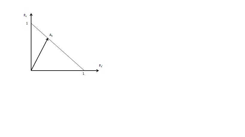
Figure 1: The probability vector ${\bf p}_{k}$ with the end at point $A_{k}$ on the simplex line determined by the equality $p_{k}+p_{k^{\prime}}=1$.

In Fig. 1, the end of the vector ${\bf p}_{k}$ coincides with the point $A_{k}$ on the line determined by the equation $p_{k}+p_{k^{\prime}}=1$. Due to the nonnegativity of numbers $p_{k}$ and $1-p_{k}$, the point belongs to the simplex. The length of the simplex line is equal to $\sqrt{2}$. Since we have three classical coins and three probability vectors ${\bf p}_{k}$, the points with coordinates $p_{1}$, $p_{2}$, and $p_{3}$ may be considered as the points either on the cube surface or inside the cube in the three-dimensional space. The length of the cube side is equal to unity.

There exists another possibility to provide the geometrical picture of the three-coin probabilities. The three simplex lines can be considered as the three sides of an equilateral triangle on the plane of equal sides $\sqrt{2}$; see Fig. 2.

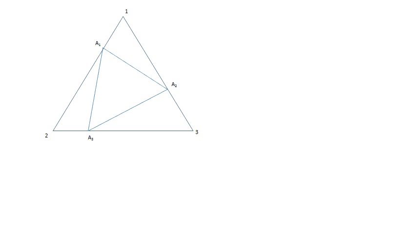
Figure 2: The equilateral triangle with vertices $1$, $2$, and $3$ and side length $\sqrt{2}$ and vertices $A_{1}$, $A_{2}$, and $A_{3}$ determining the qubit state

Thus, the points related to the cube are mapped onto the three points $A_{1}$, $A_{2}$, and $A_{3}$ on the sides of the equilateral triangle. One can connect these points by dashed lines and obtain a triangle $A_{1}A_{2}A_{3}$ with vertices $A_{1}$, $A_{2}$, and $A_{3}$ located on simplexes. This triangle can coincide with the equilateral triangle. Also the sides of this triangle can have arbitrarily small length and arbitrarily small area, if the points $A_{1}$ and $A_{2}$ or $A_{2}$ and $A_{3}$ or $A_{1}$ and $A_{3}$ are very close each to the other.

4 The Uncertainty Relation for Probabilities

For the qubit state determined by the density matrix $\rho$, the explicit form of the density matrix expressed in terms of the probabilities $p_{k}$ reads

$$\rho=\left(\begin{array}[]{cc}p_{3}&p_{1}-ip_{2}-({1}/{2})+({i}/{2})\\ p_{1}+ip_{2}-({1}/{2})-({i}/{2})&1-p_{3}\end{array}\right).$$ (6)

In terms of the probabilities $p_{k}$. two eigenvalues of the matrix $\rho$ are

$$\lambda_{1,2}=\frac{1}{2}\pm\left[\sum_{k=1}^{3}\left(p_{k}-1/2\right)^{2}\right]^{1/2};$$

they determine the Shannon entropy $H=-\lambda_{1}\ln\lambda_{1}-\lambda_{2}\ln\lambda_{2}.$

For the density matrix, we describe the properties of the triangle with vertices $A_{1}$, $A_{2}$, and $A_{3}$ located inside the equilateral triangle with the side lengths equal to $\sqrt{2}$. We assume that the vertices $A_{k}$ are closer to the $k{\mbox{th}}$ vertices of the equilateral triangle, as shown in Fig. 2. The points $A_{k}$ have the distance $d_{k}$ from the $k{\mbox{th}}$ vertices equal to $d_{k}=p_{k}\sqrt{2}.$ Since the length of the side of the equilateral triangle is equal to $\sqrt{2}$, one can calculate the lengths of the triangle sides $y_{k}$ of the triangle $A_{1}A_{2}A_{3}$; they are

$$y_{k}=\left(2+2p_{k}^{2}-4p_{k}-2p_{k+1}+2p_{k+1}^{2}+2p_{k}p_{k+1}\right)^{1/2}.$$ (7)

Now we construct three squares with sides $y_{k}$ associated with triangle $A_{1}A_{2}A_{3}$ as shown in Fig. 3.

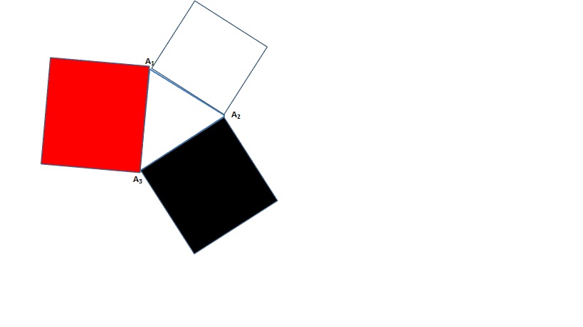
Figure 3: Triada of Malevich’s squares

The sum of the areas of these three squares is expressed in terms of the three probabilities $p_{k}$ as follows:

$$S=y_{1}^{2}+y_{2}^{2}+y_{3}^{2}=2\left[3\left(1-p_{1}-p_{2}-p_{3}\right)+2p_{1}^{2}+2p_{2}^{2}+2p_{3}^{2}+p_{1}p_{2}+p_{2}p_{3}+p_{3}p_{1}\right].$$ (8)

The three squares constructed, using the sides of the triangle, are analogs of the Triada of Malevich’s squares [27]. The properties of area $S$ given by Eq.(8) associated with the triada are different for the classical system states and for the quantum system states, namely, for three classical coins and for qubit states.

For classical coins, the numbers $p_{1}$, $p_{2}$, and $p_{3}$ take any values in the domains $0\leq p_{k}\leq 1$; this means that for statistics of classical coins the area of the Triada of Malevich’s squares satisfies the inequality

$$0\leq S\leq 6.$$ (9)

the Triada of Malevich’s squares contains the black square, the red square, and the white square [27]. For qubit states, the probabilities $0\leq p_{k}\leq 1$ to have spin projections $m=+1/2$ along three orthogonal directions satisfy the uncertainty relation inequality (1).

In view of this inequality, the area of the three Malevich’s squares can be equal to neither six nor zero but satisfies the inequality $S_{\rm min}\leq S\leq S_{\rm max}.$ For all the pure states, $|\psi_{z}\rangle=\left(\begin{array}[]{cc}1\\ 0\end{array}\right),\leavevmode\nobreak\ |\psi_{x}\rangle=\frac{1}{\sqrt{2}}\left(\begin{array}[]{cc}1\\ 1\end{array}\right),\leavevmode\nobreak\ \mbox{and}\leavevmode\nobreak\ |\psi_{y}\rangle=\frac{1}{\sqrt{2}}\left(\begin{array}[]{cc}1\\ i\end{array}\right)$ with the parameters ${\bf p}_{1}=(1/2,1/2,1)$, ${\bf p}_{2}=(1,1/2,1/2)$, and ${\bf p}_{3}=(1/2,1,1/2)$, with the area being $S=5/2$. If one chooses the probabilities $p_{1}$, $p_{2}$, and $p_{3}$ corresponding to the pure state determined by the point on the Bloch sphere, which is maximally close to the nearest vertex of the cube, the value $S=3$ will be obtained. For maximally mixed qubit state with $p_{k}=1/2$, the area $S=3/2$. The maximum and minimum values of the three Malevich’s squares correspond to the maximum and minimum values of the triangle area

$$S_{\mbox{tr}}=\frac{1}{4}\left[\left(y_{1}+y_{2}+y_{3}\right)\left(y_{1}+y_{2}-y_{3}\right)\left(y_{2}+y_{3}-y_{1}\right)\left(y_{3}+y_{1}-y_{2}\right)\right]^{1/2}.$$ (10)

The area in the case of three classical coins statistics can take zero value as the minimum, and the maximum area of the triangle is equal to ${\sqrt{3}}/{2}$. For qubit states, the triangle area has different bounds. The area for the maximally mixed qubit state is equal to $\sqrt{3}/4$; in this case, all three squares of Malevich’s triada are equal and have sides of length unity.

5 Positive and Completely Positive Maps of the Probabilities ${p_{1}}$, ${p_{2}}$, and ${p_{3}}$

In this section, we consider the map of a matrix $\rho$,

$$\rho=\left(\begin{array}[]{cc}p_{3}&p^{\ast}-\gamma^{\ast}\\ p-\gamma&1-p_{3}\end{array}\right),$$ (11)

where $p_{3}^{\ast}=p_{3}$, $p=p_{1}+ip_{2}$, and $\gamma=({1}/{2})(1+i)$, of the form

$$\rho\longrightarrow\rho_{v}=\sum_{k}V_{k}\rho V_{k}^{\dagger}.$$ (12)

Here, the matrix $V_{k}$ has the matrix elements $V_{k}=\left(\begin{array}[]{cc}V_{11}(k)&V_{12}(k)\\ V_{21}(k)&V_{22}(k)\end{array}\right)$. In the case of equalities $\sum_{k}V_{k}^{\dagger}V_{k}=1$ and $\rho=\rho^{\dagger}$, $\mbox{Tr}\rho=1$, and $\rho\geq 0$, the map given by (12) is completely positive map of the density matrix $\rho$, which provides the new density matrix $\rho_{V}$, where $\rho_{V}=\rho_{V}^{\dagger}$, $\mbox{Tr}\,\rho_{V}=1$, and $\rho_{V}\geq 0$. The map of the density matrix can be expressed in terms of the linear transform of the probabilities $p_{1}$, $p_{2}$, and $p_{3}$, i.e., for the vector

$${\bf P}=\left(\begin{array}[]{ccc}p_{3}\\ p\\ p^{\ast}\end{array}\right),$$ (13)

the map (12) provides the vector ${\bf P}_{V}$ corresponding to the density matrix $\rho_{V}$ of the form

$${\bf P}_{V}=M_{V}{\bf P}+{\bf\Delta}_{V}.$$ (14)

Here, the 3$\times$3 matrix $M_{V}$ reads

$$M_{V}=\sum_{k}\left(\begin{array}[]{ccc}|V_{11}(k)|^{2}-|V_{12}(k)|^{2}&V_{11}^{\ast}(k)V_{12}(k)&V^{\ast}_{12}(k)V_{11}(k)\\ V_{11}^{\ast}(k)V_{21}(k)-V_{12}^{\ast}(k)V_{22}(k)&V_{11}^{\ast}(k)V_{22}(k)&V_{12}^{\ast}(k)V_{21}(k)\\ V_{21}^{\ast}(k)V_{11}(k)-V_{22}^{\ast}(k)V_{12}(k)&V_{21}^{\ast}(k)V_{12}(k)&V_{22}^{\ast}(k)V_{11}(k)\end{array}\right),$$ (15)

and the vector

$${\bf\Delta}_{V}=\left(\begin{array}[]{ccc}\delta_{3}\\ \delta\\ \delta^{\ast}\end{array}\right)$$ (16)

has three components $\delta_{3}$, $\delta$, and $\delta^{\ast}$ of the form

$$\delta_{3}=\sum_{k}\left[|V_{12}(k)|^{2}-\gamma V_{11}^{\ast}(k)V_{12}(k)-\gamma^{\ast}V_{12}^{\ast}(k)V_{11}(k)\right],$$

$$\delta=\sum_{k}\left[V_{12}^{\ast}(k)V_{22}(k)-\gamma V_{11}^{\ast}(k)V_{22}(k)-\gamma^{\ast}V_{12}^{\ast}(k)V_{21}(k)+\gamma\right].$$

If the map (12) is given as the unitary map, $\rho\longrightarrow\rho_{u}=u\rho u^{\dagger},\quad uu^{\dagger}=1$, the transformed probabilities determining the density matrix $\rho_{u}$ are given by the vector

$${\bf P}_{u}=M_{u}{\bf P}+{\bf\Delta}_{u},$$ (17)

where

$$M_{u}=\left(\begin{array}[]{ccc}|u_{11}|^{2}-|u_{12}|^{2}&u_{11}^{\ast}u_{12}&u_{12}^{\ast}u_{11}\\ u_{11}^{\ast}u_{21}-u_{12}^{\ast}u_{22}&u_{11}^{\ast}u_{22}&u_{12}^{\ast}u_{21}\\ u_{21}^{\ast}u_{11}-u_{22}^{\ast}u_{12}&u_{21}^{\ast}u_{12}&u_{22}^{\ast}u_{11}\end{array}\right).$$ (18)

The shift three-vector ${\bf\Delta}_{u}$ for the unitary map has the components $\delta_{3}(u)$, $\delta(u)$, and $\delta^{\ast}(u)$ of the form

$$\delta_{3}=|u_{12}|^{2}-\gamma u_{11}^{\ast}u_{12}-\gamma^{\ast}u_{12}^{\ast}u_{11},\qquad\delta=u_{12}^{\ast}u_{22}-\gamma u_{11}^{\ast}u_{22}-\gamma^{\ast}u_{12}^{\ast}u_{21}+\gamma.$$ (19)

The 4$\times$4 matrix ${\cal M}_{u}=\left(\begin{array}[]{cc}M_{u}&{\bf\Delta}_{u}\\ 0&1\end{array}\right)$ provides an example of the representation of the group of unitary 2$\times$2 matrices satisfying the condition ${\cal M}_{u_{1}}{\cal M}_{u_{2}}={\cal M}_{u_{1}u_{2}}.$

In the process of the qubit evolution determined by the Hamiltonian $H(t)$, which can be either time-dependent or time-independent, the density matrix $\rho$ evolves by means of the unitary matrix $u(t)$. In this case, the evolution of the qubit state can be expressed as a linear transform of the probabilities $p_{3}(t)$, $p_{1}(t)$, and $p_{2}(t)$ given by (17) with matrix $M_{u(t)}$ and vector ${\bf\Delta}_{u(t)}$. The matrix elements of the matrix given by (18) and vector components of the vector given by (19) depend on the matrix elements of the unitary matrix $u_{jk}(t)$, $j,k=1,2$, if one takes into account the dependence on time.

For stationary Hamiltonian $H$ the evolution is determined by the unitary matrix $u(t)=\exp(-itH).$ If the Hamiltonian $H=H^{\dagger}$ is

$$H=\left(\begin{array}[]{cc}H_{11}&H_{12}\\ H_{21}&H_{22}\end{array}\right),$$ (20)

the matrix $u(t)$ reads

$$u(t)=\left[\cosh\alpha\left(\begin{array}[]{cc}1&0\\ 0&1\\ \end{array}\right)+\sinh\alpha\left(\begin{array}[]{cc}n_{3}&n_{1}-in_{2}\\ n_{1}+in_{2}&-n_{3}\\ \end{array}\right)\right]\exp\left[-\frac{it}{2}\left(H_{11}+H_{22}\right)\right].$$ (21)

Here, $\alpha=-ith$,

$$h=\left[\left(\frac{H_{11}-H_{22}}{2}\right)^{2}+\left(\frac{H_{12}+H_{21}}{2}\right)^{2}+\left(\frac{iH_{12}-iH_{21}}{2}\right)^{2}\right]^{1/2}$$

and

$$n_{1}=\frac{H_{12}+H_{21}}{2h},\quad n_{2}=\frac{i(H_{12}-H_{21})}{2h},\quad n_{3}=\frac{H_{11}-H_{22}}{2}.$$ (22)

For the positive map, one uses the transposition transform $\rho\longrightarrow\rho^{\mbox{tr}},$ which provides the transform of the probability

$${\bf P}\longrightarrow{\bf P}_{\mbox{tr}}=\left(\begin{array}[]{ccc}1&0&0\\ 0&0&1\\ 0&1&0\end{array}\right)\left(\begin{array}[]{ccc}p_{3}\\ p\\ p^{\ast}\end{array}\right)=\left(\begin{array}[]{ccc}p_{3}\\ p^{\ast}\\ p\end{array}\right).$$ (23)

The generic positive map gives a convex sum of vectors obtained from vector ${\bf P}$ as

$${\bf P}\longrightarrow(cos^{2}\mu){\bf P}_{V}+(\sin^{2}\mu){\bf P}_{V^{\prime}\mbox{tr}}={\bf P}_{\mbox{pos}}.$$

Here, $\mu$ is an arbitrary real parameter, ${\bf P}_{V}$ is given by (14), and ${\bf P}_{V^{\prime}\mbox{tr}}$ is

$${\bf P}_{V^{\prime}\mbox{tr}}=M_{V^{\prime}}{\bf P}_{\mbox{tr}}+{\bf\Delta}_{V^{\prime}},$$

where the matrix $M_{V^{\prime}}$ and vector ${\bf\Delta}_{V^{\prime}}$ are described by (15) and (16) determined by the matrices $V_{k}^{\prime}$.

For the transposition transform, one has $\leavevmode\nobreak\ p_{3}\longrightarrow p_{3},\quad p_{1}\longrightarrow p_{1},\quad p_{2}\longrightarrow 1-p_{2}.$ This transform corresponds to the mirror reflection of the triangle $A_{1}A_{2}A_{3}$ with respect to the mediana. The transpose matrix provides the transform of Malevich’s squares. The unitary matrix $u$ has the angles $\psi$, $\theta$, and $\phi$ as the parameters, i.e.,

$$u_{11}=\cos\,({\theta}/{2})\,\exp\big{[}{i(\phi+\psi)}/{2}\big{]},\qquad u_{12}=\sin\,({\theta}/{2})\,\exp\big{[}{i(\phi-\psi)}/{2}\big{]},$$

$$u_{21}=-\sin\,({\theta}/{2})\,\exp\big{[}{-i(\phi-\psi)}/{2}\big{]},\qquad u_{22}=\cos\,({\theta}/{2})\,\exp\big{[}{-i(\phi+\psi)}/{2}\big{]}.$$

It is easy to see that the probabilities $p_{1},\,p_{2},\,p_{3}$ depend only on two angles $\theta$ and $\psi$. The evolution of the spin state means the time dependence of angles or changes in sizes of the Malevich’s squares. Thus, an arbitrary evolution of the qubit state determined by the map $p_{1},\,p_{2},\,p_{3}\longrightarrow p_{1}(t),\,p_{2}(t),\,p_{3}(t)$ given by Eq. (14) corresponds to the time dependence of the sum of areas of Malevich’s squares (8) or the triangle area (10).

6 Conclusions

To conclude, we summarize the main results of our study.

We introduced the new geometrical interpretation of qubit states. In addition to the known picture of the qubit state given by a point in the Bloch sphere, we showed that the state can be identified with a triangle or three squares called Triada of Malevich’s squares. The area of the squares is related to quantum correlations, and the sum of areas of the squares has bounds. Also the area of the triangle has a bound. The areas are expressed in terms of three probabilities of positive spin projections on three orthogonal directions. The quantum spin-1/2 state and classical state of the three coins have different characteristics of Triada of Malevich’s squares. For classical coins, the sum of the areas of the squares takes the values $0\leq S\leq 6$. For quantum spin state, the area $S$ is larger than zero and smaller than six.

The positive maps of the qubit states (or gates used in quantum technologies) are described as linear transforms of three nonnegative probabilities $p_{1}$, $p_{2}$, and $p_{3}$. Thus, we introduced a new interpretation of qubit gates as the set of 3$\times$3 matrices and three-vectors, which form a semigroup. The semigroup of the gates transforms the Triada of Malevich’s squares into another Triada of Malevich’s squares. Also the semigroup elements (gates) transform the triangle associated with the qubit state into a triangle defining another qubit state. Any time evolution of the qubit state is described by the dynamical semigroup moving the triangle vertices $A_{1}$, $A_{2}$, and $A_{3}$. We showed that the transpose transform of the density matrix is described as the mirror reflection determined by the median of an equilateral triangle.

References

- [1] E. Schrödinger, Naturwiss., Bd. 14, s. 664 (1926).
- [2] L. D. Landau, Z. Phys., 45, 430 (1927).
- [3] J. von Neumann, Mathematische Grundlagen der Quantenmechanik, Springer, Berlin (1932).
- [4] W. Pauli, “Zur Quantenmechanik des Magnetischen Elektrons,” Z. Phys., 43, Nos. 9–10, 601–623 (1927).
- [5] V. V. Dodonov and V. I. Man’ko, Phys. Lett. A, 229, 335 (1997).
- [6] V. I. Man’ko and O. V. Man’ko, J. Exp. Theor. Phys., 85, 430 (1997).
- [7] S. Weigert, Phys. Rev. Lett., 84, 802 (2000).
- [8] J.-P. Amiet and S. Weigert, J. Opt. B: Quantum Semiclass. Opt., 1, L5 (1999).
- [9] G. M. D’Ariano, L. Maccone, and M. Paini, J. Opt. B: Quantum Semiclass. Opt., 5, 77 (2003).
- [10] O. V. Man’ko, in: B. Gruber and M. Ramek (Eds.), Proceedings of International Conference “Symmetries in Science X” (Bregenz, Austria, 1997), Plenum Press, New York (1998), p. 207.
- [11] S. N. Filippov and V. I. Man’ko, J. Russ. Laser Res., 31, 32 (2010).
- [12] O. Castanos, R. Lopes-Pena, M. A. Man’ko, and V. I. Man’ko, J. Phys. A: Math. Gen., 36, 4677 (2003).
- [13] A. B. Klimov, O. V. Man’ko, V. I. Man’ko, et al., J. Phys. A: Math. Gen., 35, 6101 (2002).
- [14] O. V. Man’ko, in: Proceedings of Wigner Centennial Conference (Pecs, Hungary, 2002), The Official Electronic Proceedings, paper 30; Acta Physica Hungarica A, Series Heavy Ion Physics, 19/3-4, 313 (2004).
- [15] V. I. Man’ko, G. Marmo, F. Ventriglia, and P. Vitale, ”Metric on the space of quantum states from relative entropy. Tomographic reconstruction” arXiv:1612.07986 (2016).
- [16] Y. Shalibo, R. Resh, O. Fogel, et al., Phys. Rev. Lett., 110, 100404 (2013).
- [17] M. H. Devoret and R. J. Schoelkopf, Superconducting Circuits for Quantum Information: An Outlook, Science, 339, 1169 (2013).
- [18] Y. A. Pashkin, T. Yamamoto, O. Astafiev, et al., Nature, 421, 823 (2003).
- [19] A. Averkin, A. Karpov, K. Shulga, et al., Rev. Sci. Instrum., 85, 104702 (2014).
- [20] O. V. Man’ko, V. I. Man’ko, and G. Marmo, Phys. Scr., 62, 446 (2000).
- [21] R. L. Stratonovich, J. Exp. Theor. Phys., 5, 1206 (1957).
- [22] O. V. Man’ko, V. I. Man’ko, and G. Marmo, J. Phys. A: Math. Gen., 35, 699 (2002).
- [23] O. V. Man’ko, V. I. Man’ko, G. Marmo, and P. Vitale, Phys. Lett. A, 360, 522 (2007).
- [24] F. Lizzi and P. Vitale, SIGMA, 10, 36 (2014).
- [25] A. Ibort, V. I. Man’ko, G. Marmo, et al., Phys. Scr., 79, 065013 (2009).
- [26] M. Asorey, A. Ibort, G. Marmo, and F. Ventriglia, Phys. Scr., 90, 074031 (2015).
- [27] Aleksandra Shatskikh, Black Square: Malevich and the Origin of Suprematism, Yale University Press, New Haven (2012).