Multiple Sclerosis Lesion Segmentation from Brain MRI via Fully Convolutional Neural Networks

Abstract

Multiple Sclerosis (MS) is an autoimmune disease that leads to lesions in the central nervous system. Magnetic resonance (MR) images provide sufficient imaging contrast to visualize and detect lesions, particularly those in the white matter. Quantitative measures based on various features of lesions have been shown to be useful in clinical trials for evaluating therapies. Therefore robust and accurate segmentation of white matter lesions from MR images can provide important information about the disease status and progression. In this paper, we propose a fully convolutional neural network (CNN) based method to segment white matter lesions from multi-contrast MR images. The proposed CNN based method contains two convolutional pathways. The first pathway consists of multiple parallel convolutional filter banks catering to multiple MR modalities. In the second pathway, the outputs of the first one are concatenated and another set of convolutional filters are applied. The output of this last pathway produces a membership function for lesions that may be thresholded to obtain a binary segmentation. The proposed method is evaluated on a dataset of $100$ MS patients, as well as the ISBI 2015 challenge data consisting of $14$ patients. The comparison is performed against four publicly available MS lesion segmentation methods. Significant improvement in segmentation quality over the competing methods is demonstrated on various metrics, such as Dice and false positive ratio. While evaluating on the ISBI 2015 challenge data, our method produces a score of $90.48$, where a score of $90$ is considered to be comparable to a human rater.

1 Introduction

Multiple Sclerosis (MS) is an autoimmune disease of the central nervous system, in which inflammatory demyelination of axons causes focal lesions to occur in the brain. White matter lesions in MS can be detected with standard magnetic resonance imaging (MRI) acquisition protocols without contrast injection. It has been shown that many features of lesions, such as volume Kalincik et al. (2012) and location Sati and et. al. (2016), are important biomarkers of MS, and can be used to detect disease onset or track its progression. Therefore accurate segmentation of white matter lesions is important in understanding the progression and prognosis of the disease. With $T_{2}$-w FLAIR (fluid attenuated inversion recovery) imaging sequences, most lesions appear as bright regions in MR images, which helps its automatic segmentation. Therefore FLAIR is the most common imaging contrast for detection of MS lesions and is often used in conjunction with other structural MR contrasts, including $T_{1}$-w, $T_{2}$-w, or $PD$-w images. Although manual delineations are considered as the gold standard, manually segmenting lesions from 3D images is tedious, time consuming, and often not reproducible. Therefore automated lesion segmentation from MRI is an active area of development in MS research.

Automated lesion segmentation in MS is a challenging task for various reasons: (1) the lesions are highly variable in terms of size and location, (2) lesion boundaries are often not well defined, particularly on FLAIR images, and (3) clinical quality FLAIR images may possess low resolution and often have imaging artifacts. It has also been observed that there is very high inter-rater variability even with experienced raters Carass and et. al. (2017); Egger et al. (2017). Therefore there is an inherent reliability challenge associated with lesion segmentation. This problem is accentuated by the fact that MRI does not have any uniform intensity scale (like CT); acquisition of images in different scanners and with different contrast properties can therefore add to the complexity of segmentation.

Many automated lesion segmentation methods have been proposed in the past decade Garcia-Lorenzo et al. (2013). There are usually two broad categories of segmentations, supervised and unsupervised. Unsupervised lesion segmentation methods rely on intensity models of brain tissue, where image voxels containing high intensities in FLAIR images are modeled as outliers Garcia-Lorenzo et al. (2011); Shiee et al. (2009) based on the intensity distributions. The outlier voxels then become potential candidates for lesions and then the segmentation can be refined by a simple threshold Souplet et al. (2008); Roura et al. (2015); Jain et al. (2015). Alternatively, Bayesian models such as mixtures of Gaussians Schmidt et al. (2012); Strumia et al. (2016); Leemput et al. (2001); Sudre et al. (2015) or Student’s t mixture models Freire and Ferrari (2016) can be applied on the intensity distributions of potential lesions and normal tissues. Optimal segmentation is then achieved via an expectation-maximization algorithm. Additional information about intensity distributions and expected locations of normal tissues via a collection of healthy subjects Tomas-Fernandez and Warfield (2015) can be included to determine the lesions more accurately. Local intensity information can also be included via Markov random field to obtain a smooth segmentation Harmouche et al. (2006, 2015).

Supervised lesion segmentation methods make use of atlases or templates, which typically consist of multi-contrast MR images and their manually delineated lesions. As seen in the ISBI-2015 lesion segmentation challenge Carass and et. al. (2017), supervised methods have become more popular and are usually superior to unsupervised ones, with $4$ out of top $5$ methods being supervised. These methods learn the transformation from the MR image intensities to lesion labels (or memberships) on atlases, and then the learnt transformation is applied onto a new unseen image to generate its lesion labels. Logistic regression Sweeney et al. (2013); Dworkin et al. (2016) and support vector machines Lao et al. (2008) have been used in lesion classification, where features include voxel-wise intensities from multi-contrast images and the classification task is to label an image voxel as lesion or non-lesion. Instead of using voxel-wise intensities, patches have been shown to be a robust and useful feature Roy et al. (2014). Random forest Maier et al. (2015); Geremia et al. (2011); Jog et al. (2015) and k-nearest neighbors Griffanti et al. (2016) based algorithms have used patches and other features, computed at a particular voxel, to predict the label of that voxel. Dictionary based methods Roy et al. (2015b, a); Guizard et al. (2015); Deshpande et al. (2015) use image patches from atlases to learn a patch dictionary that can sufficiently describe potential lesion and non-lesion patches. For a new unseen patch, similar patches are found from the dictionary and combined with weights based on the similarity.

In recent years, convolutional neural networks (CNN), also known as deep learning LeCun et al. (2015), have been successfully applied to many medical image processing applications Greenspan et al. (2016); Litjens et al. (2017). CNN based methods produce state-of-the-art results in many computer vision problems such as object detection and recognition Szegedy et al. (2015). The primary advantage of neural networks over traditional machine learning algorithms is that CNNs do not need hand-crafted features, making it applicable to a diverse set of problems when it is not obvious what features are optimal. Because neural networks can handle 3D images or image patches, both 2D Roth et al. (2016) and 3D Brosch et al. (2016) algorithms have been proposed, with 2D patches often being preferred for memory and speed efficiency. With advancements in graphics processor units (GPU), neural network models can be trained in a GPU within a fraction of time taken by that with multiple CPUs. Also CNNs can handle very large datasets without incurring too much increase in processing time. Therefore they have gained popularity in the medical imaging community in solving increasingly difficult problems.

CNNs have been shown to be better or on par with both probabilistic and multi-atlas label fusion based methods for whole brain segmentation on adult Wachinger et al. (2017); Moeskops et al. (2016b); Chen et al. (2017) and neonatal brains Zhang et al. (2015); Moeskops et al. (2016a). They have been especially successful in tumor segmentations Kamnitsas et al. (2017); Pereira et al. (2016); Casamitjana et al. (2016), as seen on the BRATS 2015 challenge Menze and et. al. (2015). They have recently been applied for brain extraction in the presence of tumors Kleesiek et al. (2016). Missing image contrasts pose a significant challenge in medical imaging, where not all available image contrasts may not be acquired for all subjects. Traditional CNN architectures can be modified to include image statistics in addition to image intensities to circumvent missing image contrasts Havaei et al. (2016) without sacrificing too much accuracy. CNN models have also been applied to segment both cross-sectional Prieto et al. (2017); Yoo et al. (2014); Ghafoorian et al. (2017a, b); Moeskops et al. (2017) and longitudinal Birenbaum and Greenspan (2016) lesions from multi-contrast MR images. Recently, a two-step cascaded CNN architecture Valverde et al. (2017) has been proposed, where two separate networks are learnt; the first one computes an initial lesion membership based on MR images and manual segmentations, while the second one refines the segmentation from the first network by including its false positives in the training samples.

In this paper, we propose a fully convolutional neural network model, called Fast Lesion EXtraction using COnvolutional Neural Networks (FLEXCONN), to segment MS lesions, where parallel pathways of convolutional filters are first applied to multiple contrasts. The outputs of those pathways are then concatenated and another set of convolutional filters is applied on the joined output. Similar to Ghafoorian et al. (2017b), we used large 2D patches and show that larger patches produce more accurate results compared to smaller patches. The paper is organized as follows. First the experimental data is described in Sec. 2. The proposed FLEXCONN network architecture and its various parameter optimizations are described in Sec. 3. The segmentation results and the comparison with other methods are described in Sec. 4.

Table 1: Short description of the four datasets is presented here. Details can be found in Sec. 2. For ISBI-21 and ISBI-61, each image has two manual lesion masks from two raters.

Dataset	#Images	#Masks	Usage	Availability
ISBI-21	21	42	Training	Public
VAL-28	28	28	Validation	Private
ISBI-61	61	122	Testing	Private
MS-100	100	100	Testing	Private

Table 2: Imaging parameters, such as repetition time $T_{R}$ (ms), echo time $T_{E}$(ms), inversion time $T_{I}$ (ms), flip angle, and resolution (mm³) are shown. These parameters are same for all datasets described in Sec. 2.

	$T_{R}$	$T_{E}$	$T_{I}$	Flip	Resolution
				Angle
3D MPRAGE	10.3	6	835	8°	$0.82\times 0.82\times 1.17$
$T_{2}$-w	4177	12.31	N/A	90°	$0.82\times 0.82\times 2.2$
$PD$-w	$4177$	80	N/A	90°	$0.82\times 0.82\times 2.2$
2D FLAIR	$11000$	68	2800	90°	$0.82\times 0.82\times 2.2$
					& $0.82\times 0.82\times 4.4$

2 Materials

Two sets of data are used to evaluate the proposed algorithm. The first dataset is from the ISBI 2015 challenge Carass and et. al. (2017), which includes two groups, training and testing. The training group, denoted by ISBI-21, is publicly available and comprises $21$ scans from $5$ subjects. Four of the subjects have $4$ time-points and one has $5$ time-points, each time-point separated by approximately a year. The test group, denoted by ISBI-61, is not public and has $14$ subjects with $61$ images, each subject with $4-5$ time-points, each time-point also being separated by a year. Although these images actually contain longitudinal scans of the same subject, we treat the dataset as a cross-sectional study and report numbers on each image separately since longitudinal information is not used within our approach. A short description of the datasets is provided in Table 1.

The second dataset consists of $128$ patients enrolled in a natural history study of MS, $79$ with relapsing-remitting, $30$ with secondary progressive, and $19$ with primary progressive MS. For experimentation purpose, we arbitrarily divided this dataset into two groups, validation ($n=28$) and test ($n=100$), denoted as VAL-28 and MS-100 respectively. The proposed algorithm as well as the other competing methods were trained using ISBI-21 as training data. Then various parameters, as described in Sec. 3.4, were optimized using VAL-28 as the validation set. Finally the optimized algorithms were compared on the ISBI-61 and MS-100 datasets, as detailed in Sec. 4.1 and Sec. 4.2.

Each subject from both datasets had $T_{1}$-w MPRAGE, $T_{2}$-w, $PD$-w, and FLAIR images acquired in a Philips 3T scanner. The imaging parameters are listed in Table 2. Each image in MS-100 and VAL-28 has one manually delineated lesion segmentation mask. Every image in ISBI-21 and ISBI-61 has two masks, drawn by two different raters, as explained in Carass et al. (2011).

3 Method

3.1 Image Preprocessing

The $T_{1}$-w images of every subject in the MS-100 and VAL-28 dataset were first rigidly registered Avants et al. (2011) to the axial $1$ mm³ MNI template Oishi et al. (2008). They were then skullstripped Carass et al. (2011); Roy et al. (2017) and corrected for any intensity inhomogeneity by N4 Tustison et al. (2010). The other contrasts, i.e. $T_{2}$-w, $PD$-w, and FLAIR images were then registered to the $T_{1}$-w image in MNI space, stripped with the same skull-stripping mask, and corrected by N4 after stripping.

The preprocessing steps for the ISBI-21 and ISBI-61 datasets were very similar and detailed in Carass and et. al. (2017). Briefly, the $T_{1}$-w images of the baseline of every subject were rigidly registered to the MNI template, skullstripped Carass et al. (2011), and corrected by N4. Then the other contrasts of the baseline and all contrasts of the followup time-points were rigidly registered to the baseline $T_{1}$-w and corrected by N4. Lesions for both data sets were manually delineated on pre-processed FLAIR images, although the other contrasts were available for reference.

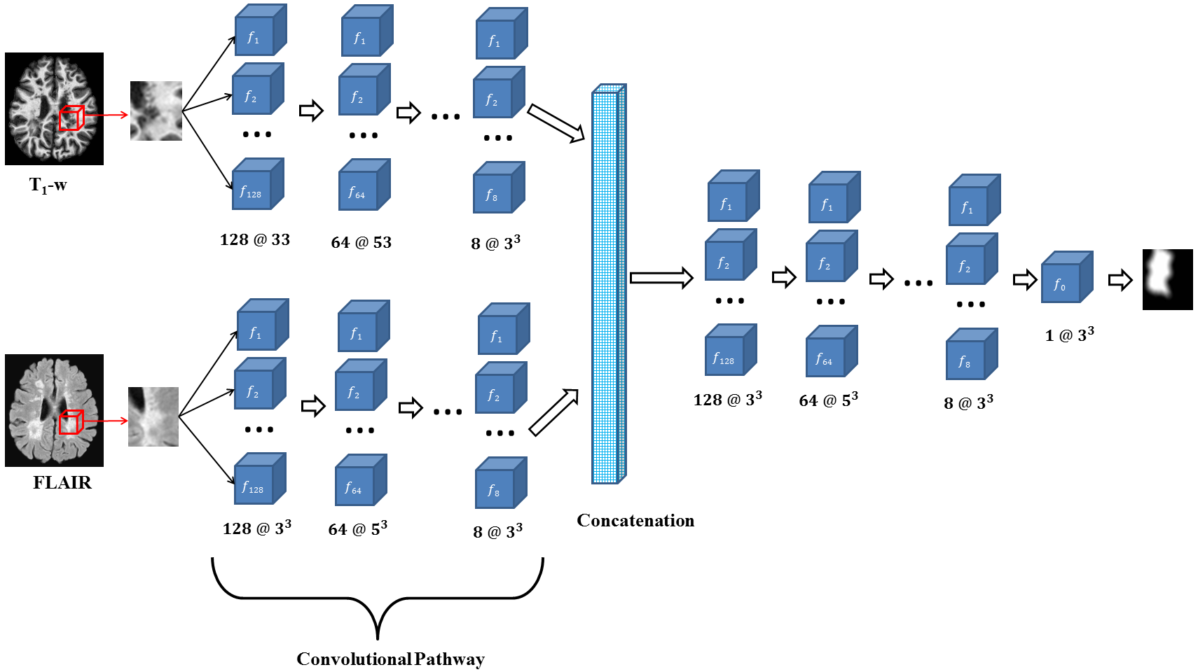
Figure 1: Proposed neural network architecture for lesion segmentation is shown. 2D patches from multi-channel images are used as features and convolutional filters ($f_{j},j=1,2,\ldots$) are first applied in parallel. Here $j$ denotes the index of the filter. Note that each “filter ($f_{j}$)” includes a convolution and a ReLU module. The filter outputs are concatenated and passed through another convolutional pathway to predict a membership function of the patch. The filter number and sizes are shown as $128\ @\ 3^{2}$, indicating the corresponding filter bank contains $128$ filters, each with size $3\times 3$.

3.2 CNN Architecture

Cascade type neural network architectures have become popular in medical image segmentation, where features are either 2D slices or 3D patches from MR images. Typically, multi-channel patches are first independently passed through convolutional filter banks, then a fully connected (FC) layer is applied to predict the voxel-wise membership at the center of the patches Wachinger et al. (2017) from the concatenated outputs of the filters. We follow a similar architecture, shown in Fig. 1, where multi-channel 2D $p_{1}\times p_{2}$ patches are convolved with multiple filter banks of various sizes (called a “convolutional pathway”), and the outputs of the convolutional pathways are concatenated. The details of a convolutional pathway is given in Table 3. After concatenation, instead of an FC layer to predict the membership or probability of the center voxel of the $p_{1}\times p_{2}$ patch, we add another convolutional pathway that predicts a membership value of the whole $p_{1}\times p_{2}$ patch. Note that with variable pad sizes (see Table 3), the sizes of the input and outputs of the filters are kept identical to the original MR image patch size. The training memberships are generated by simply convolving the manual hard segmentations with a $3\times 3$ (denoted $3^{2}$) Gaussian kernel. We observed that larger patches produce mored accurate segmentations compared to smaller patches, and determined that a $35\times 35$ patch produced the best results based on the VAL-28 dataset. The estimation of the optimal patch size is described in Sec. 3.4.

Table 3: Filter parameters of a convolutional pathway, as shown in Fig. 1, are provided. Every size is in voxels. Note that with variable pad sizes, the input and output size of the filters are kept identical to the training patch size $p_{1}\times p_{2}$.

Filter	Type	Number	Filter Size	Pad Size	Parameters	# Parameters
Bank		of Filters
1	Convolution	128	$3^{2}$	$1^{2}$	$3\times 3\times 128$	1152
2	Convolution	64	$5^{2}$	$2^{2}$	$5\times 5\times 128\times 64$	204800
3	Convolution	32	$3^{2}$	$1^{2}$	$3\times 3\times 64\times 32$	18432
4	Convolution	16	$5^{2}$	$2^{2}$	$5\times 5\times 32\times 16$	12800
5	Convolution	8	$3^{2}$	$1^{2}$	$3\times 3\times 16\times 8$	1152

MPRAGE	FLAIR	Manual	With FC	Without FC

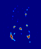
Figure 2: Example of lesion memberships are shown when generated with a fully connected (FC) layer predicting memberships at a voxel, compared to the proposed model where patch based memberships are predicted using convolutional pathways. Note that a FC layer produces fuzzier memberships and potentially more false positives. Memberships are scaled between $0$ (dark blue) and $1$ (red).

Improved segmentation results were achieved using a set of $5$ convolutional filter banks with decreasing numbers of filters in one convolutional pathway, as shown in Fig. 1 and Table 3. The optimal number of filter banks in a pathway was also estimated from a validation strategy discussed in Sec. 3.4. Each convolution is followed by a rectified linear unit (ReLU) Nair and Hinton (2010). The combination of convolution and ReLU is indicated by $f_{j}$ in Fig. 1. Our experiments showed that smaller filter sizes such as $3^{2}$ and $5^{2}$ generally produce better segmentation than bigger filters (such as $7^{2}$ and $9^{2}$), which was also observed before Simonyan and Zisserman (2015). We hypothesize that since lesion boundaries are often not well defined, small filters tend to capture the boundaries better. Also the number of free parameters ($9$ for $3^{2}$) increases for larger filters ($49$ for $7^{2}$), which in turn can either decrease the stability of the result or incur overfitting. However, smaller filters may perform worse for larger lesions. Therefore we empirically used a combination of $3^{2}$ and $5^{2}$ filters based on our validation set VAL-28.

As noted, a major difference in the network architecture proposed here in contrast to other popular CNN based segmentation methods is the use of a convolutional layer to predict membership functions. The advantages of such a configuration compared to a FC layer are as follows:

1. Depending on the number of convolutions and the patch size, the number of free parameters for a FC layer can be large, thereby increasing the possibility of overfitting. Recent successful deep learning networks such as ResNet He et al. (2016b) and GoogLeNet Szegedy et al. (2015) have put more focus on fully convolutional networks and networks, with ResNet having no FC layer at all. Although dropout Srivastava et al. (2014) has been proposed to reduce the effect of overfitting a network to the training data, the mechanism of randomly turning off different neurons inherently results in slightly different segmentations every time the training is performed even with the same training data.

2. We observed that memberships predicted with an FC layer result in more false positives compared to a fully convolutional network. An example is shown in Fig. 2, where lesion memberships are generated from MPRAGE and FLAIR using the proposed model of convolutional pathways and a comparable model where the last convolutional pathway after concatenation (see Fig. 1) is replaced with a FC layer predicting voxel-wise memberships. The membership image generated with an FC layer, although being close to $1$ inside the lesions, has high values ($\geq 0.5$) in the left and right frontal cortex where the FLAIR image shows some artifacts. However, the membership obtained with the proposed method shows relatively low values near the frontal cortex.

3. With FC layer, voxel-wise predictions are performed for each voxel on a new image. Therefore the prediction time for the whole image comprising millions of voxels can take some time even on a GPU, as mentioned in Wachinger et al. (2017). In contrast, with fully convolutional prediction, lesion membership estimation of a $1$ mm³ MR volume of size $181\times 217\times 181$ takes only a couple of seconds. Note that although patches are used for training, the final trained model contains only convolution filters and does not depend in any way on the input patch size. Therefore during testing, the lesion membership of a whole 2D slice, irrespective of the slice size, is predicted at a time by applying convolutions on the whole slice. Without an FC layer, the images need not be decomposed into sub-regions, e.g., Kamnitsas et al. (2017). Consequently, there is no need to employ membership smoothing between sub-regions. In addition, since the training memberships, generated by Gaussian blurring of hard segmentations, are smooth, the resultant predicted memberships are also smooth (Fig. 2 last column).

MS lesions are heavily under-represented as a tissue class in a brain MR image, compared to GM or WM. In the training dataset ISBI-21, lesions represent on an average $1$% of all brain tissue voxels. For a binary lesion classification, most supervised machine learning algorithms thus require balanced training data He and Garcia (2009), where number of patches with lesions are approximately equal to lesion free patches. Therefore normal tissue patches are randomly undersampled Valverde et al. (2017); Roy et al. (2015b) to generate a balanced training dataset. This is true for a small $5^{2}$ or $7^{2}$ patch, which may have all or most voxels as lesions, thereby requiring some other patches with all or most voxels as normal tissue. In Sec. 3.4, we show that using larger patches, such as $25\times 25$ or $35\times 35$, produce more accurate segmentations compared to smaller $9^{2}$ or $13^{2}$ patches. Since we use large patches which cover most of the largest lesions, the effect of data imbalance is reduced.

With large patches, our training data consists of patches where the center voxel of a patch has a lesion label, i.e., all lesion patches are included in the training data with a stride of $1$. We do not include any normal tissue patches, where none of the voxels have a lesion label. Experiments showed that inclusion of the normal tissue patches does not improve segmentation accuracy, but incurs longer training time by requiring more training epochs to achieve similar accuracy. However, one drawback of only including patches with lesions is that generally more training data are required, especially when the number of lesions become much less than number of parameters to be optimized, as shown in Table 3.

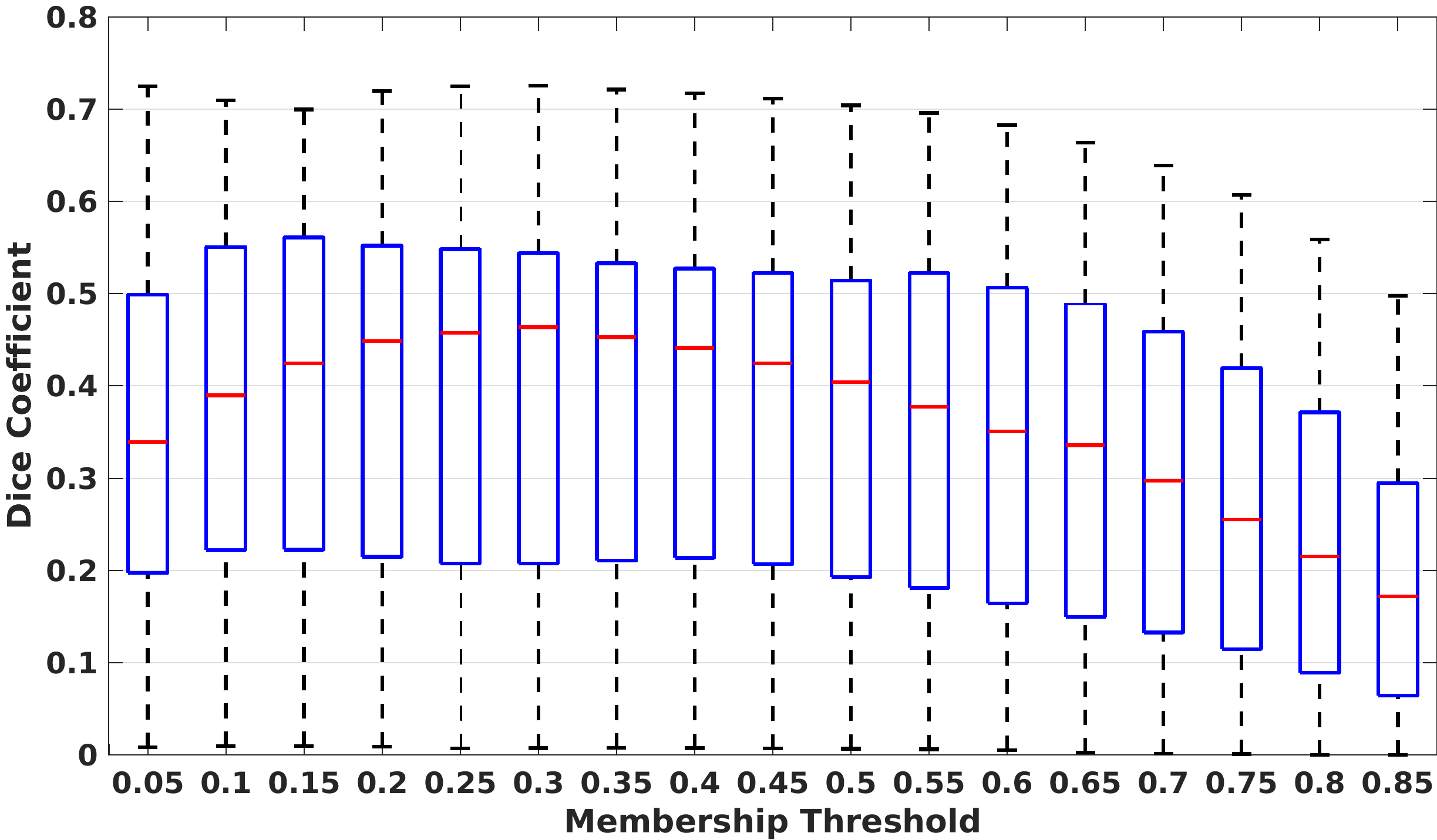
Figure 3: Dice coefficients of segmentations from VAL-28 dataset are shown at different membership thresholds from $0.05$ to $0.85$. The highest median Dice was observed at $0.30$. See Sec. 3.4 for details.

MPRAGE	T2	PD	FLAIR	Manual
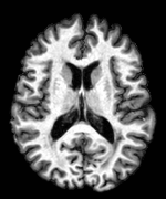
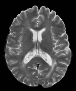
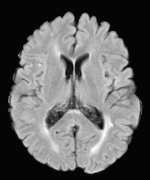
$13\times 13$	$17\times 17$	$19\times 19$	$31\times 31$	$35\times 35$

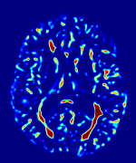
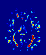
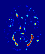
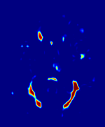
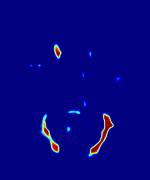
Figure 4: Memberships of a subject from VAL-28 dataset with various patch sizes are shown. As the patch size increases, the false positives in the cortex begins to decrease.

3.3 Comparison Metrics

We chose $4$ comparison metrics: Dice coefficient, lesion false positive rate (LFPR), positive predictive value (PPV), and absolute volume difference (VD) to compare segmentations. For a manual and an automated binary segmentation $\mathcal{M}$ and $\mathcal{A}$ respectively, Dice is a voxel-wise overlap measure defined as,

$$\mathrm{Dice}(\mathcal{A},\mathcal{M})=\frac{2|\mathcal{A}\cap\mathcal{M}|}{|\mathcal{A}|+|\mathcal{M}|},$$

where $|\cdot|$ denotes number of non-zero voxels. Since lesions are often small and their total volumes are typically very small ($1-2$%) compared to the whole brain volume, Dice can be affected by the low volume of the segmentations Geremia et al. (2011). Therefore LFPR is defined based on distinct lesion counts. A distinct lesion is defined as an $18$-connected object, although such a description of lesions may or may not be biologically accurate. LFPR is the number of lesions in the automated segmentation that do not overlap with any lesions in the manual segmentation, divided by the total number of lesions in the automated segmentation. Two lesions are considered overlapped when they share at least one voxel. PPV is defined as the ratio of true positive voxels and total number of positive voxels, expressed as

$$\mathrm{PPV}(\mathcal{A},\mathcal{M})=\frac{2|\mathcal{A}\cap\mathcal{M}|}{|\mathcal{A}|},$$

Absolute volume difference is defined as

$$\mathrm{VD}(\mathcal{A},\mathcal{M})=\frac{\mathrm{abs}(|\mathcal{A}|-|\mathcal{M}|)}{|\mathcal{M}|}.$$

All statistical tests were performed with a non-parametric paired Wilcoxon signed rank test.

3.4 Parameter Optimization

In this section, we describe a validation strategy to optimize user selectable parameters of the proposed network: (1) patch size, (2) number of filter banks in a convolutional pathway, and (3) the final threshold to create hard segmentations from memberships. After training with ISBI-21, the network was applied to the images of VAL-28 to generate their lesion membership images. Memberships were thresholded and then masked with a cerebral white matter mask Shiee et al. (2009) to remove any residual false positives. Dice was used as the primary metric for optimizing the parameters, with LFPR used as a secondary metric for patch size optimization. Although our model is capable of using all four available contrasts, initial experiments on VAL-28 data showed negligible improvement in segmentation accuracy with $T_{2}$-w and $PD$-w images. Therefore all results were obtained with only MPRAGE and FLAIR contrasts.

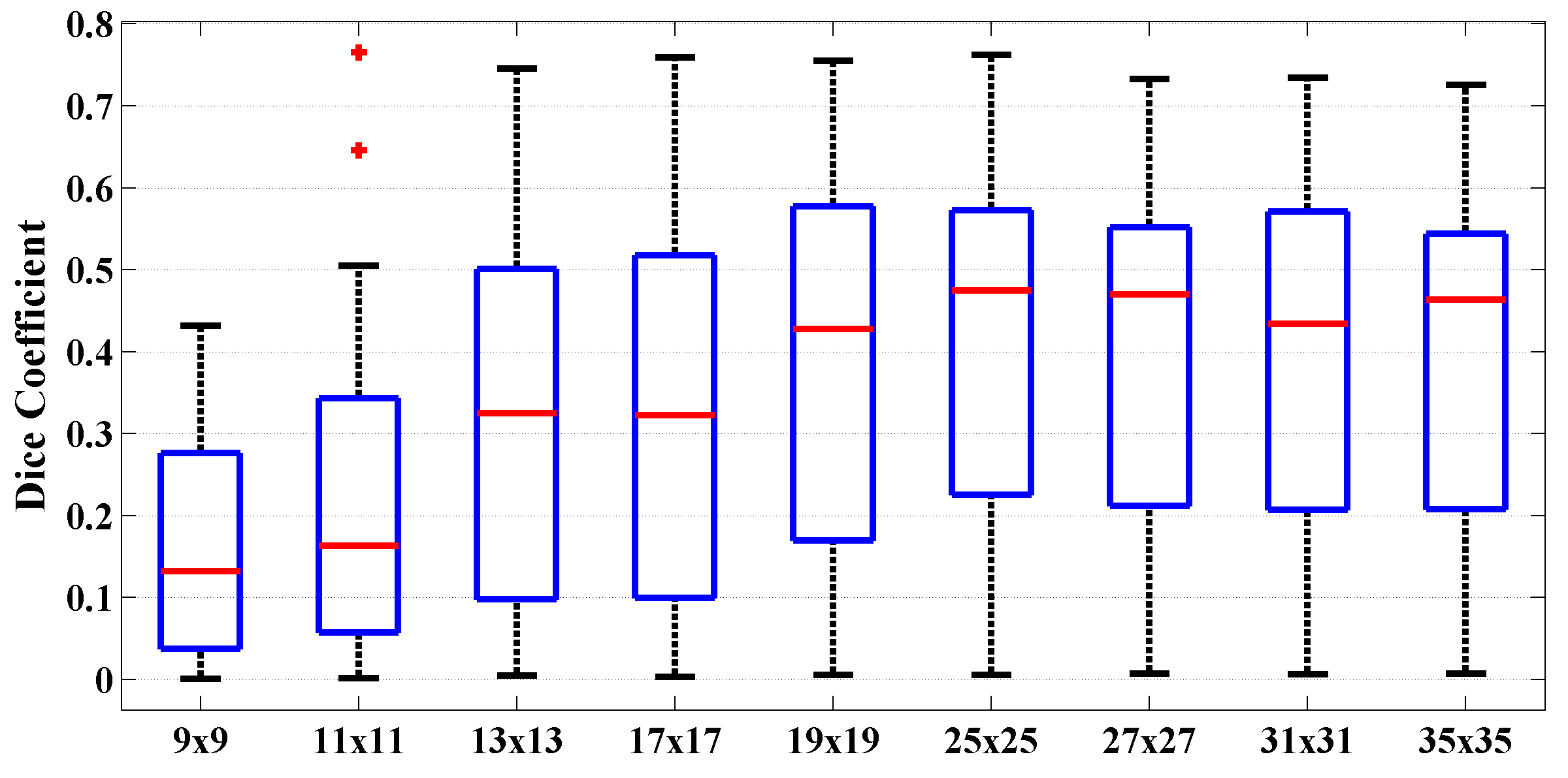
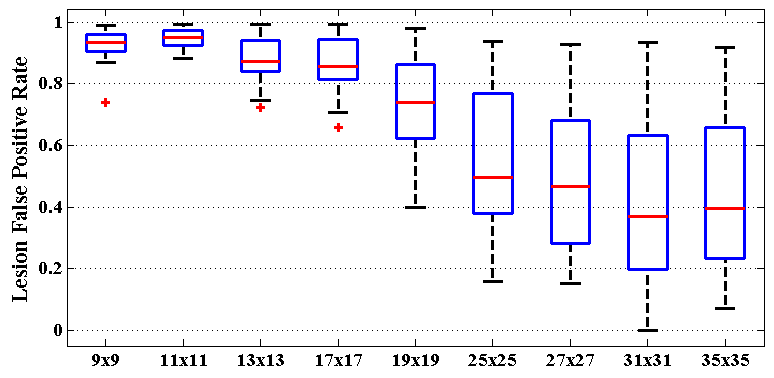
Figure 5: Dice coefficients (top) and LFPR (bottom) are plotted for the segmentations of VAL-28 data when trained with ISBI-21 for various patch sizes. See Sec. 3.4 for details.

To optimize the membership threshold, we trained a network with $35\times 35$ patches. Memberships generated on VAL-28 were segmented with thresholds from $0.05$ to $0.85$ with an increment of $0.05$. The range of Dice coefficients is shown in Fig. 3. The highest median Dice coefficient was observed for a threshold of $0.30$. This is intuitively reasonable because during training, the lesion memberships of atlases were generated from their hard segmentations using a $3\times 3$ Gaussian kernel, and it can be shown that the half max of a $3\times 3$ discrete Gaussian is at $0.31$.

Next we varied the depth of a convolutional pathway from $2$ to $6$ filter banks while keeping the number of filters as a multiple of $2$, with the last filter bank having $8$ filters. The highest median Dice coefficient was observed at a depth of $5$, which is significantly larger than Dice coefficients with depths $3$ and $4$ ($p<0.05$). Although the differences in Dice coefficients were small between various depths, we used a depth of $5$ for the rest of the experiments. With more than $6$ filter banks, the Dice slowly decreases, which can be attributed to overfitting the training data.

Patch size is another important parameter of the network. In computer vision applications such as object detection, usually a whole 2D image is used as a feature. However, full 3D medical images can not typically be used because of memory limitations. Fig. 4 shows examples of lesion memberships obtained with different sized 2D patches. As the patch sizes increases, the false positives that are mostly observed in the cortex tend to decrease. Fig. 5 shows a plot of Dice and LFPR with various patch sizes, ordered from left to right according to their increasing size. Note that smaller patches ($9^{2}$ to $17^{2}$) produced significantly lower Dice and higher LFPR compared to other patches ($p<0.001$), as seen from the memberships in Fig. 4. Also some of the highest Dice and lowest LFPR were observed for patches with large in-plane size, i.e., $31\times 31$, $27\times 27$, and $35\times 35$. It was observed in Fig. 5 that there is no significant difference between Dice coefficients for $31\times 31$, $35\times 35$, or $27\times 27$, but LFPR of both $35\times 35$ and $31\times 31$ are significantly lower than that of $27\times 27$ ($p<0.05$). We chose $35\times 35$ as the optimal patch size. Other choices of smaller $5^{2}$ and $7^{2}$ patches (not shown) yielded worse results. Note that although training was performed with different patch sizes, the memberships were generated slice by slice, as the trained model consisted only of convolutions and did not need any information about patch sizes.

3.5 Competing Methods

We compared FLEXCONN with LesionTOADS Shiee et al. (2009), OASIS Sweeney et al. (2013), LST Schmidt et al. (2012), and S3DL Roy et al. (2015b). LesionTOADS (Topology reserving Anatomy Driven Segmentation) does not need any parameter tuning and uses MPRAGE and FLAIR. OASIS (OASIS is Automated Statistical Inference for Segmentation) has a threshold parameter that is used to threshold the memberships to create a hard segmentation. It was optimized as $0.15$ by training a logistic regression on the ISBI-21 and applying the regression model to VAL-28. A similar value was reported in the original paper. OASIS requires all four contrasts, MPRAGE, $T_{2}$-w, $PD$-w, and FLAIR. LST (Lesion Segmentation Toolbox) has a parameter $\kappa$, which initializes the lesion segmentation. Lower values of $\kappa$ produces bigger lesions. We optimized $\kappa$ to maximize the Dice coefficient on VAL-28 data and found that $\kappa=0.10$ yielded the highest median Dice. LST uses MPRAGE and FLAIR images. S3DL has two parameters, number of atlases and membership threshold. We observed that adding more than $4$ atlases did not improve Dice coefficients significantly, as was reported in the original paper. Hence we used $5$ atlases as the last time-points of the $5$ subjects from the ISBI-21 dataset. The optimal threshold for S3DL was also found to be $0.80$. S3DL used MPRAGE and FLAIR as adding $T_{2}$-w and $PD$-w images did not improve the segmentation.

3.6 Implementation Details

Our model was implemented in Tensorflow and Keras. We used Adam Kingma and Ba (2015) as the optimizer, which has been shown to produce the fastest convergence in neural network parameter optimization. The optimization was run with fixed learning rate of $0.0001$ for $20$ epochs, which was empirically found to produce sufficient convergence without overfitting. During training with $35\times 35$ patches using lesions from $21$ subjects of ISBI-21 dataset, we used $20$% of the total number patches for validation and the remaining $80$% for training. Training with $128$ minibatches required about $6$ hours on an Nvidia Titan X GPU with $12$ GB memory. Segmenting a new subject took $3-5$ seconds.

4 Results

In this section, we show comparison of FLEXCONN with other methods on two datasets MS-100 and ISBI-61 (see Section 2). Research code implementing our method is freely available.

4.1 MS-100 Dataset

For this dataset, the training was performed separately with two sets of masks from the two raters of ISBI-21 data. Then two memberships were generated for each of the $100$ images. For each image, the two memberships were averaged and thresholded to form the final segmentation. Fig. 6 shows MR images and segmentations of $3$ subjects from the MS-100 dataset, where the subjects have high ($22$cc), moderate ($8$cc), and low ($1$cc) lesion loads. For the subject with high lesion loads (#1), all $5$ methods performed comparably, although OASIS and LST underestimated some small and subtle lesions (yellow arrow). For the subject with moderate lesion load (#2), OASIS and S3DL underestimated some lesions (orange arrow) and LesionTOADS overestimated some (green arrow). When the lesion load is small and the FLAIR image has some artifacts (subject #3), LesionTOADS, S3DL, and OASIS produce a false positive (yellow arrow) in the cortex. LST shows underestimation, but FLEXCONN does not produce the false positive. The reason is partly because of the use of large patches, which can successfully distinguish between bright voxels in cortex and peri-ventricular regions.

LesionTOADS	S3DL	OASIS	LST	Proposed

Manual vs automated lesion volumes for the $5$ methods on MS-100 dataset. The solid lines show robust linear fits of the points and the dotted black line represents the unit slope line. Numbers are in mm³.

Table 4: Slopes and intercepts from Fig. 4.1 are shown for the MS-100 dataset. Bold indicates the largest absolute value among the $5$ methods.

Method	Slope	Intercept (cc)
LesionTOADS Shiee et al. (2009)	0.6112	7783.2
S3DL Roy et al. (2015b)	0.7488	1570.1
OASIS Sweeney et al. (2013)	0.8002	1163.1
LST Schmidt et al. (2012)	0.4650	-44.9
FLEXCONN	0.9421	143.2

Median values of Dice, lesion false positive rate (LFPR), positive predictive value (PPV), and volume difference (VD) are shown for competing methods on MS-100 dataset. Bold indicates significantly highest/lowest $(p<0.05)$ number. See Sec. 3.3 for the definition of the metrics.

	Dice	LFPR	PPV	VD
LesionTOADS	0.4678	0.6865	0.3968	0.4718
S3DL	0.5526	0.4164	0.5968	0.2755
OASIS	0.4993	0.5081	0.6242	0.2681
LST	0.4239	0.4409	0.7820	0.5623
FLEXCONN	0.5639	0.3077	0.6040	0.1978

	MPRAGE	FLAIR	$\mathbf{T_{2}}$-w	$\mathbf{PD}$-w	Manual
Subject #1

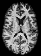
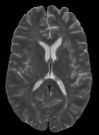
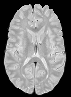
LesionTOADS	S3DL	OASIS	LST	FLEXCONN	Membership

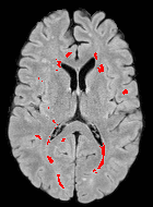
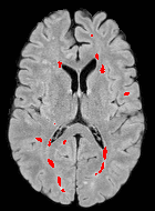
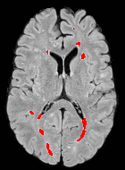
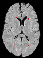
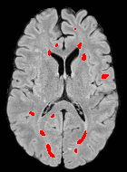
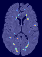
	MPRAGE	FLAIR	$\mathbf{T_{2}}$-w	$\mathbf{PD}$-w	Manual
Subject #2

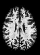
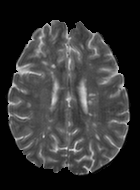
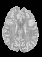
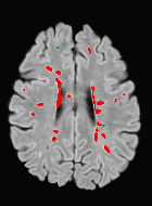
LesionTOADS	S3DL	OASIS	LST	FLEXCONN	Membership

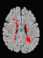
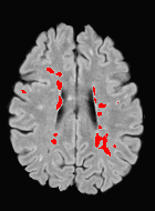
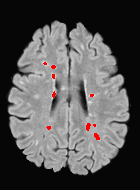
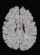
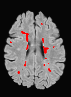
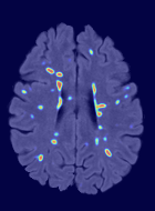
	MPRAGE	FLAIR	$\mathbf{T_{2}}$-w	$\mathbf{PD}$-w	Manual
Subject #3

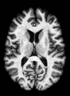
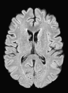
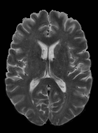
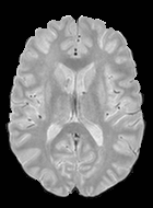
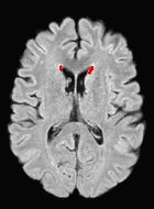
LesionTOADS	S3DL	OASIS	LST	FLEXCONN	Membership

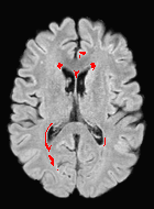
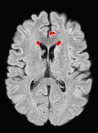
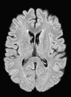
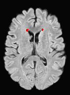
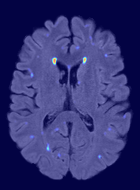
Figure 6: $T_{1}$-w, $T_{2}$-w, $PD$-w, and FLAIR images of three subjects with high, medium, and low lesion load from MS-100 dataset, along with segmentations from $5$ competing methods and one lesion membership from the proposed CNN based FLEXCONN.

MPRAGE	FLAIR	Rater 1	Rater 2

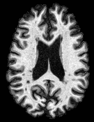
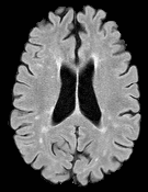
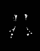
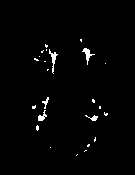
Membership#1	Membership#2	FLEXCONN

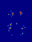
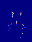
Figure 7: A typical segmentation example for one subject from the ISBI-61 dataset. Membership#1 and #2 refer to the lesion memberships obtained using training data from rater 1 and 2, respectively.

Mean values of comparison metrics are shown for various competing methods on ISBI-61 dataset. Bold indicates highest or lowest value. See Sec. 3.3 for the definition of the metrics. The score was computed as a weighted average of the other metrics.

	Dice	LFPR	PPV	VD	Score
Birenbaum et. al.Birenbaum and Greenspan (2016)	0.6271	0.4976	0.7890	0.3523	90.07
Jain et. al.Jain et al. (2015)	0.5243	0.4005	0.6947	0.3886	88.74
Tomas-Fernandez et. al.Tomas-Fernandez and Warfield (2015)	0.4317	0.4116	0.6974	0.5110	87.07
Gghafoorian et. al.Ghafoorian et al. (2017a)	0.5009	0.5766	0.5942	0.5708	86.92
Sudre et. al.Sudre et al. (2015)	0.5226	0.6776	0.6690	0.3887	86.44
Maier et. al.Maier et al. (2015)	0.6050	0.2658	0.7746	0.3654	90.28
Deshpande et. al.Deshpande et al. (2015)	0.5920	0.2806	0.7622	0.3214	89.81
Valverde et. al.Valverde et al. (2017)	0.6305	0.1529	0.7867	0.3385	91.33
FLEXCONN	0.5243	0.1103	0.8660	0.5207	90.48

Since lesion volume is an important outcome measure for evaluating disease progression, we compared automated lesion volume vs the manual lesion volume in Fig. 4.1. Solid lines represent a robust linear fit of the points, and the black dotted line represents unit slope. It is observed that LesionTOADS (blue) overestimates lesions when lesion load is small, and LST (magenta) underestimates the lesion when the lesion load is high. S3DL, OASIS, and FLEXCONN show less bias with respect to lesion load, while FLEXCONN has the slope closest to unity ($0.94$). The slopes and intercepts with manual lesion volumes are also shown in Table 4. Table 4.1 shows median values of various comparison metrics for the $5$ competing methods. FLEXCONN produces significantly better Dice, LFPR, and VD ($p<0.01$) among the four methods. LST produces the highest PPV.

4.2 ISBI-61 Dataset

Although ISBI-61 includes longitudinal images, we performed the segmentation in a cross-sectional manner. The segmentations were generated in a similar fashion as the MS-100 dataset (Sec. 4.1) by averaging two memberships obtained using two sets of training. A typical segmentation example is shown in Fig. 7, where the subject has high lesion load ($40$cc).

Table 4.1 shows a comparison with some of the methods that participated in the ISBI 2015 challenge. The proposed method achieves the lowest LFPR ($0.1102$) and the highest PPV ($0.866$) compared to others, while the highest Dice was produced by another recent CNN based method Valverde et al. (2017). The lowest VD was achieved by a dictionary based method Deshpande et al. (2015). To rank a method, a score was computed using a weighted average of various metrics including Dice, LFPR, PPV, and VD, as detailed in Carass and et. al. (2017). For the two raters, the inter-rater score was $0.67$, which is scaled to $90$. Therefore, a score of $90$ or more indicates segmentation accuracy similar to the consistency between two human raters. FLEXCONN achieved a score of $90.48$, while the other CNN based methods, Valverde et al. (2017) and Birenbaum and Greenspan (2016), achieved scores of $91.33$ and $90.07$, respectively, indicating their performance to be comparable to human raters. Most of the top scoring methods in the challenge were based on CNN.

5 Discussion

We have proposed a simple end-to-end fully convolutional neural network based method to segment MS lesions from multi-contrast MR images. Our network is does not have any fully connected layers and after training, takes only a couple of seconds to segment lesions on a new image. Although we validated using only $T_{1}$-w and FLAIR contrasts, other contrasts can easily be included in the framework. We have shown that using large, two-dimensional, patches provide significantly better segmentations than smaller patches. Comparisons with four other publicly available lesion segmentation methods, two supervised and two unsupervised, showed superior performance over $100$ images.

During training, there were several parameters that were empirically determined. First, for a $(2w+1)^{2}$ filter, we used $w^{2}$ zero padding at each convolution so as to have a uniform input and output patch size to all filters. Without padding, the output size after every filter bank decreases and care should be taken to keep the input and output patches properly aligned. With padding, we can add or remove filter banks without worrying about alignment. Another important parameter is the batch size. With too small a batch size, the gradient computation becomes noisy and the stochastic gradient descent optimization may not lead to a local minima. With too large a batch size, the optimization may lead to a sharp local minima, making the model not generalizable to new data Keskar et al. (2016). Therefore, an appropriate batch size should be chosen based on the data. During training, we empirically chose $128$ for training and $64$ as a test batch size.

With the removal of fully connected layers, the proposed fully convolutional network can generate the membership of a 2D slice without the need for dividing images into sub-regions Kamnitsas et al. (2017). With large enough patches, the contextual information of a lesion voxel can be obtained from within the patch. This is representative of a human observer looking at a large neighborhood while considering a voxel to be lesion of not. Note that although the training is performed with patches, the prediction step does not need the patch information because the trained convolutions are applied to a whole 2D slice. As a consequence, the memberships are inherently smooth, and the problem of possible discontinuities between sub-regions does not arise.

MS lesion segmentation is associated with high inter-rater variability in manual delineations, as seen on both the MICCAI 2008 and ISBI 2015 challenges. For example, in the MICCAI 2008 lesion segmentation challenge, the average Dice overlap between two raters was $0.25$, and in the ISBI 2015 challenge, the inter-rater Dice overlap was $0.63$ Carass and et. al. (2017). Therefore it is expected that the average Dice coefficients of the proposed segmentations are as low as $0.5$ and sometimes are even lower. However, Dice coefficients can be artificially low when the actual lesion volume is small, therefore having fewer false positives can be more desirable than having a high Dice. Our proposed model had the lowest false positive rate compared to all other methods on both test datasets while maintaining good sensitivity.

In our experiments, we used large 2D patches similar to Ghafoorian et al. (2017b), in comparison to isotropic 3D patches as used before, e.g., $11^{3}$ in Valverde et al. (2017), $23^{3}$ in Wachinger et al. (2017), and $17^{3}$ in Kamnitsas et al. (2017). The rationale behind using large anisotropic patches is twofold. First, experiments with full 3D isotropic $9^{3}$ or $11^{3}$ patches showed little or no improvement in Dice and led to increased false positives, with memberships similar to the one with $13\times 13$ patches, as shown in Fig. 4. Larger isotropic patches, e.g. $19^{3}$ or $25^{3}$, showed inferior segmentation, and in some cases, optimization did not converge. The reason is that the FLAIR images in the test datasets had inherently low resolution in the inferior-superior direction, $2.2$ mm and $4.4$ mm compared to in-plane resolution of $0.82\times 0.82$ mm. Therefore 2D axial patches capture the high resolution in-plane information that represents the original thick axial slices. Second, the lesions are usually focal and small in size, unlike other brain structures. Therefore a very large isotropic patch around a small lesion can include superfluous information about the lesion, which can increase the amount of false positives. Note that with in more recent studies employing high resolution 3D FLAIR sequences, it is trivial to extend the algorithm to accommodate for 3D patches.

One drawback of the proposed method is that it requires a large number of training patches. With the ISBI-21 as training data, there are approximately only $270,000$ training patches. Patch rotation Guizard et al. (2015) is a standard data augmentation technique where training patches are rotated by $45$°, $90$°, $135$°, and $180\degree$ in the axial plane, and added to the training patch set in addition to the non-rotated patches. Our initial experiments with rotated patches on the VAL-28 dataset showed only $1-2$% increase in average Dice coefficients with rotated patches at the cost of significantly more memory and training time, indicating that the network is already sufficiently generalizable with the original training data. Therefore we did not use rotated patches in the final segmentation. However, further experiments are needed to understand the full scope of performance improvement with respect to the available training data and other augmentation techniques, such as patch cropping or adding visually imperceptible jitters to images.

Table 4.1 shows that there is no single method that has the highest metrics among the six. This is consistent with previously reported results Carass and et. al. (2017) on the same ISBI-61 data. There are several methods with score more than $90$, such as Birenbaum and Greenspan (2016); Maier et al. (2015); Valverde et al. (2017). Valverde et al. (2017) produced the highest Dice, while FLEXCONN produced the highest LFPR and PPV. Both these methods are based on CNN, outperforming other traditional machine learning based algorithms. Note that FLEXCONN has a very simple network architecture and does not have a longitudinal component like Birenbaum and Greenspan (2016) or two-pass correction mechanism like Valverde et al. (2017). Still it was able to achieve similar overall performance. Future work will include further comparison with other CNN based methods such as Ghafoorian et al. (2017a); Valverde et al. (2017); Birenbaum and Greenspan (2016). We will also explore more recent and state-of-the-art networks such as Szegedy et al. (2015); He et al. (2016a, b) to achieve better accuracy and temporal consistency in segmentations.

6 Acknowledgements

Support for this work included funding from the Department of Defense in the Center for Neuroscience and Regenerative Medicine and intramural research program at NIH and NINDS. This work was also partially supported by grant from National MS Society RG-1507-05243 and NIH R01NS082347.

References

- Avants et al. (2011) Avants, B. B., Tustison, N. J., Song, G., Cook, P. A., Klein, A., Gee, J. C., 2011. A reproducible evaluation of ANTs similarity metric performance in brain image registration. NeuroImage 54 (3), 2033– 2044.
- Birenbaum and Greenspan (2016) Birenbaum, A., Greenspan, H., 2016. Longitudinal multiple sclerosis lesion segmentation using multi-view convolutional neural networks. In: Intl. Workshop on Deep Learning in Medical Image Analysis. pp. 58–67.
- Brosch et al. (2016) Brosch, T., Tang, L. Y. W., Yoo, Y., Li, D. K. B., Traboulsee, A., Tam, R., 2016. Deep 3d convolutional encoder networks with shortcuts for multiscale feature integration applied to multiple sclerosis lesion segmentation. IEEE Trans. Med. Imag. 35 (5), 1229–1239.
- Carass et al. (2011) Carass, A., Cuzzocreo, J., Wheeler, M. B., Bazin, P. L., Resnick, S. M., Prince, J. L., 2011. Simple paradigm for extra-cerebral tissue removal: Algorithm and analysis. NeuroImage 56 (4), 1982– 1992.
- Carass and et. al. (2017) Carass, A., et. al., 2017. Longitudinal multiple sclerosis lesion segmentation: resource & challenge. NeuroImage 148, 77 –102.
- Casamitjana et al. (2016) Casamitjana, A., Puch, S., Aduriz, A., Vilaplana, V., 2016. 3d convolutional neural networks for brain tumor segmentation: A comparison of multi-resolution architectures. In: Intl. Workshop on Brainlesion: Glioma, Multiple Sclerosis, Stroke and Traumatic Brain Injuries. pp. 150–161.
- Chen et al. (2017) Chen, H., Dou, Q., Yu, L., Qin, J., Heng, P.-A., 2017. Voxresnet: Deep voxelwise residual networks for brain segmentation from 3D MR images. NeuroImage 00, 00.
- Deshpande et al. (2015) Deshpande, H., Maurel, P., Barillot, C., 2015. Adaptive dictionary learning for competitive classification of multiple sclerosis lesions. In: Intl. Symp. on Biomed. Imag. (ISBI). pp. 136–139.
- Dworkin et al. (2016) Dworkin, J. D., Sweeney, E. M., Schindler, M. K., Chahin, S., Reich, D. S., Shinohara, R. T., 2016. PREVAIL: Predicting recovery through estimation and visualization of active and incident lesions. NeuroImage: Clinical 12, 293–299.
- Egger et al. (2017) Egger, C., Opfer, R., Wang, C., Kepp, T., Sormani, M. P., Spies, L., Barnett, M., Schippling, S., 2017. MRI FLAIR lesion segmentation in multiple sclerosis: Does automated segmentation hold up with manual annotation? NeuroImage 13, 264–270.
- Freire and Ferrari (2016) Freire, P. G., Ferrari, R. J., 2016. Automatic iterative segmentation of multiple sclerosis lesions using Student’s t mixture models and probabilistic anatomical atlases in FLAIR images. Computers in Biology and Medicine 73, 10–23.
- Garcia-Lorenzo et al. (2013) Garcia-Lorenzo, D., Francis, S., Narayanan, S., Arnold, D. L., Collins, D. L., 2013. Review of automatic segmentation methods of multiple sclerosis white matter lesions on conventional magnetic resonance imaging. Med. Image Anal. 17 (1), 1 –18.
- Garcia-Lorenzo et al. (2011) Garcia-Lorenzo, D., Prima, S., Arnold, D. L., Collins, L. D., Barillot, C., 2011. Trimmed-likelihood estimation for focal lesions and tissue segmentation in multisequence MRI for multiple sclerosis. IEEE Trans. Med. Imag. 30 (8), 1455 –1467.
- Geremia et al. (2011) Geremia, E., Clatz, O., Menze, B. H., Konukoglu, E., Criminisi, A., Ayache, N., 2011. Spatial decision forests for MS lesion segmentation in multi-channel magnetic resonance images. NeuroImage 57 (2), 378–390.
- Ghafoorian et al. (2017a) Ghafoorian, M., Karssemeijer, N., Heskes, T., Bergkamp, M., Wissink, J., Obels, J., Keizer, K., de Leeuw, F.-E., van Ginneken, B., Marchiori, E., Platel, B., 2017a. Deep multi-scale location-aware 3D convolutional neural networks for automated detection of lacunes of presumed vascular origin. NeuroImage: Clinical 14, 391–399.
- Ghafoorian et al. (2017b) Ghafoorian, M., Karssemeijer, N., Heskes, T., van Uden, I. W. M., Sanchez, C. I., Litjens, G., de Leeuw, F. E., van Ginneken, B., Marchiori, E., Platel, B., 2017b. Location sensitive deep convolutional neural networks for segmentation of white matter hyperintensities. Scientific Reports 7, 5110.
- Greenspan et al. (2016) Greenspan, H., van Ginneken, B., Summers, R. M., 2016. Guest editorial deep learning in medical imaging: Overview and future promise of an exciting new technique. IEEE Trans. Med. Imag. 35 (5), 1153–1159.
- Griffanti et al. (2016) Griffanti, L., Zamboni, G., Khan, A., Li, L., Bonifacio, G., Sundaresan, V., Schulz, U. G., Kuker, W., Battaglini, M., Rothwell, P. M., 2016. BIANCA (Brain Intensity AbNormality Classification Algorithm): A new tool for automated segmentation of white matter hyperintensities. NeuroImage 141, 191 205.
- Guizard et al. (2015) Guizard, N., Coupe, P., Fonov, V. S., Manjon, J. V., Arnold, D. L., Collins, D. L., 2015. Rotation-invariant multi-contrast non-local means for MS lesion segmentation. NeuroImage: Clinical 8, 376 –389.
- Harmouche et al. (2006) Harmouche, R., Collins, L., Arnold, D., Francis, S., Arbel, T., 2006. Bayesian MS Lesion Classification Modeling Regional and Local Spatial Information. IEEE Intl. Conf. Patt. Recog. 3, 984–987.
- Harmouche et al. (2015) Harmouche, R., Subbanna, N. K., Collins, D. L., Arnold, D. L., Arbel, T., 2015. Probabilistic multiple sclerosis lesion classification based on modeling regional intensity variability and local neighborhood information. IEEE Trans. Biomed. Engg. 62 (5), 1281–1292.
- Havaei et al. (2016) Havaei, M., Guizard, N., Chapados, N., Bengio, Y., 2016. HeMIS: Hetero-modal image segmentation. In: Med. Image Comp. and Comp. Asst. Intervention (MICCAI). pp. 469–477.
- He and Garcia (2009) He, H., Garcia, E. A., 2009. Learning from imbalanced data. IEEE Trans. Knowledge and Data Engineering 21 (9), 1263–1284.
- He et al. (2016a) He, K., Zhang, X., Ren, S., Sun, J., 2016a. Deep residual learning for image recognition. In: Intl. Conf. on Comp. Vision. and Patt. Recog. (CVPR). pp. 770–778.
- He et al. (2016b) He, K., Zhang, X., Ren, S., Sun, J., 2016b. Identity mappings in deep residual networks. In: European Conf. on Comp. Vision (ECCV). pp. 630–645.
- Jain et al. (2015) Jain, S., Sima, D. M., Ribbens, A., Cambron, M., Maertens, A., Hecke, W. V., Mey, J. D., Barkhof, F., Steenwijk, M. D., Daams, M., Maes, F., Huffel, S. V., Vrenken, H., Smeets, D., 2015. Automatic segmentation and volumetry of multiple sclerosis brain lesions from MR images. NeuroImage: Clinical 8 (5), 1229–1239.
- Jog et al. (2015) Jog, A., Carass, A., Pham, D. L., Prince, J. L., 2015. Multi-output decision trees for lesion segmentation in multiple sclerosis. In: Proceedings of SPIE Medical Imaging (SPIE). Vol. 9413. p. 94131C.
- Kalincik et al. (2012) Kalincik, T., Vaneckova, M., Tyblova, M., Krasensky, J., Seidl, Z., Havrdova, E., Horakova, D., 2012. Volumetric MRI markers and predictors of disease activity in early multiple sclerosis: A longitudinal cohort study. PLoS One 7 (11), e50101.
- Kamnitsas et al. (2017) Kamnitsas, K., Ledig, C., Newcombe, V. F., Simpson, J. P., Kane, A. D., Menon, D. K., Rueckert, D., Glocker, B., 2017. Efficient multi-scale 3D CNN with fully connected CRF for accurate brain lesion segmentation. Med. Image Anal. 36, 61– 78.
- Keskar et al. (2016) Keskar, N. S., Mudigere, D., Nocedal, J., Smelyanskiy, M., Tang, P. T. P., 2016. On large-batch training for deep learning: Generalization gap and sharp minima. arXiv preprint arXiv:1609.04836.
- Kingma and Ba (2015) Kingma, D. P., Ba, J., 2015. Adam: A method for stochastic optimization. In: Intl. Conf. on Learning Representations (ICLR).
- Kleesiek et al. (2016) Kleesiek, J., Urban, G., Hubert, A., Schwarz, D., Maier-Hein, K., Bendszus, M., Biller, A., 2016. Deep MRI brain extraction: A 3D convolutional neural network for skull stripping. NeuroImage 129, 460–469.
- Lao et al. (2008) Lao, Z., Shen, D., Liu, D., Jawad, A. F., Melhem, E. R., Launer, L. J., Bryan, R. N., Davatzikos, C., 2008. Computer-assisted segmentation of white matter lesions in 3D MR images, using support vector machine. Academic Radiology 15 (3), 300–313.
- LeCun et al. (2015) LeCun, Y., Bengio, Y., Hinton, G., 2015. Deep learning. Nature 521 (7553), 436 444.
- Leemput et al. (2001) Leemput, K. V., Maes, F., Vandermeulen, D., Colchester, A., Suetens, P., 2001. Automated segmentation of multiple sclerosis lesions by model outlier detection. IEEE Trans. Med. Imag. 20 (8), 677–688.
- Litjens et al. (2017) Litjens, G., Kooi, T., Bejnordi, B. E., Setio, A. A. A., Ciompi, F., Ghafoorian, M., van der Laak, J. A., van Ginneken, B., Sanchez, C. I., 2017. A survey on deep learning in medical image analysis. Med. Image Anal. 42, 60–88.
- Maier et al. (2015) Maier, O., Wilms, M., von der Gablentz, J., Kramer, U. M., Munte, T. F., Handels, H., 2015. Extra tree forests for sub-acute ischemic stroke lesion segmentation in MR sequences. Journal of Neuroscience Methods 89, 89–100.
- Menze and et. al. (2015) Menze, B. H., et. al., 2015. The multimodal brain tumor image segmentation benchmark (BRATS). IEEE Trans. Med. Imag. 34 (10), 1993– 2024.
- Moeskops et al. (2017) Moeskops, P., de Bresser, J., Kuijf, H., Mendrik, A., Biessels, G., Pluim, J. P. W., Isgum, I., 2017. Evaluation of a deep learning approach for the segmentation of brain tissues and white matter hyperintensities of presumed vascular origin in MRI. NeuroImage: Clinical 00, 00–00.
- Moeskops et al. (2016a) Moeskops, P., Viergever, M. A., Mendrik, A. M., de Vries, L. S., Benders, M. J. N. L., Isgum, I., 2016a. Automatic segmentation of MR brain images with a convolutional neural network. IEEE Trans. Med. Imag. 35 (5), 1252–1261.
- Moeskops et al. (2016b) Moeskops, P., Wolterink, J. M., Velden, B. H. M. v., Gilhuijs, K. G. A., Leiner, T., Viergever, M. A., Isgum, I., 2016b. Deep learning for multi-task medical image segmentation in multiple modalities. In: Med. Image Comp. and Comp. Asst. Intervention (MICCAI). pp. 478–486.
- Nair and Hinton (2010) Nair, V., Hinton, G. E., 2010. Rectified linear units improve restricted boltzmann machines. In: Intl. Conf. on Machine Learning (ICML). pp. 807–814.
- Oishi et al. (2008) Oishi, K., Zilles, K., Amunts, K., Faria, A., Jiang, H., Li, X., Akhter, K., Hua, K., Woods, R., Toga, A. W., Pike, G. B., Rosa-Neto, P., Evans, A., Zhang, J., Huang, H., Miller, M. I., van Zijl, P. C., Mazziotta, J., Mori, S., 2008. Human brain white matter atlas: identification and assignment of common anatomical structures in superficial white matter. NeuroImage 43 (3), 447–457.
- Pereira et al. (2016) Pereira, S., Pinto, A., Alves, V., Silva, C. A., 2016. Brain tumor segmentation using convolutional neural networks in MRI images. IEEE Trans. Med. Imag. 35 (5), 1240–1251.
- Prieto et al. (2017) Prieto, J. C., Cavallari, M., Palotai, M., Pinzon, A. M., Egorova, S., Styner, M., Guttmann, C. R. G., 2017. Large deep neural networks for MS lesion segmentation. In: Proceedings of SPIE Medical Imaging (SPIE). Vol. 10133. p. 10133F.
- Roth et al. (2016) Roth, H. R., Lu, L., Liu, J., Yao, J., Seff, A., Cherry, K., Kim, L., Summers, R. M., 2016. Improving computer-aided detection using convolutional neural networks and random view aggregation. IEEE Trans. Med. Imag. 35 (5), 1170–1181.
- Roura et al. (2015) Roura, E., Oliver, A., Cabezas, M., Valverde, S., Pareto, D., Vilanova, J. C., Ramio-Torrenta, L., Rovira, A., Llado, X., 2015. A toolbox for multiple sclerosis lesion segmentation. Neuroradiology 57, 1031– 1043.
- Roy et al. (2017) Roy, S., Butman, J. A., Pham, D. L., Alzheimers Disease Neuroimaging Initiative, 2017. Robust skull stripping using multiple MR image contrasts insensitive to pathology. NeuroImage 146, 132 –147.
- Roy et al. (2015a) Roy, S., Carass, A., Prince, J. L., Pham, D. L., 2015a. Longitudinal patch-based segmentation of multiple sclerosis white matter lesions. In: Machine Learning in Medical Imaging. Vol. 9352. pp. 194–202.
- Roy et al. (2014) Roy, S., He, Q., Carass, A., Jog, A., Cuzzocreo, J. L., Reich, D. S., Prince, J. L., Pham, D. L., 2014. Example based lesion segmentation. In: Proceedings of SPIE Medical Imaging (SPIE). Vol. 9034. p. 90341Y.
- Roy et al. (2015b) Roy, S., He, Q., Sweeney, E., Carass, A., Reich, D. S., Prince, J. L., Pham, D. L., 2015b. Subject specific sparse dictionary learning for atlas based brain MRI segmentation. IEEE Journal of Biomedical and Health Informatics 19 (5), 1598–1609.
- Sati and et. al. (2016) Sati, P., et. al., 2016. The central vein sign and its clinical evaluation for the diagnosis of multiple sclerosis: a consensus statement from the North American Imaging in Multiple Sclerosis Cooperative. Nature Rev. Neurology 12, 714 –722.
- Schmidt et al. (2012) Schmidt, P., Gaser, C., Arsic, M., Buck, D., Forschler, A., Berthele, A., Hoshi, M., Ilg, R., Schmid, V. J., Zimmer, C., Hemmer, B., Muhlau, M., 2012. An automated tool for detection of FLAIR-hyperintense white-matter lesions in multiple sclerosis. NeuroImage 59 (4), 3774–3783.
- Shiee et al. (2009) Shiee, N., Bazin, P. L., Ozturk, A., Reich, D. S., Calabresi, P. A., Pham, D. L., 2009. A Topology-Preserving Approach to the Segmentation of Brain Images with Multiple Sclerosis Lesions. NeuroImage 49 (2), 1524– 1535.
- Simonyan and Zisserman (2015) Simonyan, K., Zisserman, A., 2015. Very deep convolutional networks for large-scale image recognition. In: Intl. Conf. on Learning Representations (ICLR).
- Souplet et al. (2008) Souplet, J., Lebrun, C., Ayache, N., Malandain, G., 2008. An automatic segmentation of T2-FLAIR multiple sclerosis lesions. In: Multiple Sclerosis Lesion Segmentation Challenge Workshop (MICCAI 2008 Workshop).
- Srivastava et al. (2014) Srivastava, N., Hinton, G., Krizhevsky, A., Sutskever, I., Salakhutdinov, R., 2014. Dropout: A simple way to prevent neural networks from overfitting. J. Machine Learning Research 15 (1), 1929–1958.
- Strumia et al. (2016) Strumia, M., Schmidt, F. R., Anastasopoulos, C., Granziera, C., Krueger, G., Brox, T., 2016. White matter MS-lesion segmentation using a geometric brain model. IEEE Trans. Med. Imag. 35 (2), 1636–1646.
- Sudre et al. (2015) Sudre, C. H., Cardoso, M. J., Bouvy, W. H., Biessels, G. J., Barnes, J., Ourselin, S., 2015. Bayesian model selection for pathological neuroimaging data applied to white matter lesion segmentation. IEEE Trans. Med. Imag. 34 (10), 2079–2102.
- Sweeney et al. (2013) Sweeney, E. M., Shinohara, R. T., Shiee, N., Mateen, F. J., Chudgar, A. A., Cuzzocreo, J. L., Calabresi, P. A., Pham, D. L., Reich, D. S., 2013. OASIS is automated statistical inference for segmentation, with applications to multiple sclerosis lesion segmentation in MRI. NeuroImage: Clinical 2, 402 413.
- Szegedy et al. (2015) Szegedy, C., Liu, W., Jia, Y., Sermanet, P., Reed, S., Anguelov, D., Erhan, D., Vanhoucke, V., Rabinovich, A., 2015. Going deeper with convolutions. In: Intl. Conf. on Comp. Vision. and Patt. Recog. (CVPR). pp. 1–9.
- Tomas-Fernandez and Warfield (2015) Tomas-Fernandez, X., Warfield, S. K., 2015. A model of population and subject (MOPS) intensities with application to multiple sclerosis lesion segmentation. IEEE Trans. Med. Imag. 34 (6), 1349–1361.
- Tustison et al. (2010) Tustison, N. J., Avants, B. B., Cook, P. A., Zheng, Y., Egan, A., Yushkevich, P. A., Gee, J. C., 2010. N4ITK: improved N3 bias correction. IEEE Trans. Med. Imag. 29 (6), 1310–1320.
- Valverde et al. (2017) Valverde, S., Cabezasa, M., Roura, E., Gonz lez-Villaa, S., Pareto, D., Vilanova, J. C., Ramio-Torrenta, L., Rovira, A., Oliver, A., Llado, X., 2017. Improving automated multiple sclerosis lesion segmentation with a cascaded 3d convolutional neural network approach. NeuroImage 155, 159 –168.
- Wachinger et al. (2017) Wachinger, C., Reuter, M., Klein, T., 2017. DeepNAT: Deep convolutional neural network for segmenting neuroanatomy. NeuroImage 00 (00), 00.
- Yoo et al. (2014) Yoo, Y., Brosch, T., Traboulsee, A., Li, D. K., Tam, R., 2014. Deep learning of image features from unlabeled data for multiple sclerosis lesion segmentation. In: Machine Learning in Medical Imaging. Vol. 8679. pp. 117 –124.
- Zhang et al. (2015) Zhang, W., Li, R., Deng, H., Wang, L., Lin, W., Ji, S., Shen, D., 2015. Deep convolutional neural networks for multi-modality isointense infant brain image segmentation. NeuroImage 108, 214 224.