The inf-sup condition and error estimates of the Nitsche method for evolutionary diffusion-advection-reaction equations

Abstract

The Nitsche method is a method of “weak imposition” of the inhomogeneous Dirichlet boundary conditions for partial differential equations. This paper explains stability and convergence study of the Nitsche method applied to evolutionary diffusion-advection-reaction equations. We mainly discuss a general space semidiscrete scheme including not only the standard finite element method but also Isogeometric Analysis. Our method of analysis is a variational one that is a popular method for studying elliptic problems. The variational method enables us to obtain the best approximation property directly. Actually, results show that the scheme satisfies the inf-sup condition and Galerkin orthogonality. Consequently, the optimal order error estimates in some appropriate norms are proven under some regularity assumptions on the exact solution. We also consider a fully discretized scheme using the backward Euler method. Numerical example demonstrate the validity of those theoretical results.

Key words: diffusion-advection-reaction equation, inf-sup condition, IGA

2010 Mathematics Subject Classification: 65M12, 65M60

1 Introduction

The boundary condition is an indispensable component of the well-posed problem of partial differential equations. It is not merely a side condition. In computational mechanics, great attention should be paid the imposition of boundary conditions, although it is sometimes understood as a simple and unambiguous task.

The Neumann boundary condition or natural boundary condition is naturally considered in the variational equation so that it is handled directly in finite element method (FEM). By contrast, a specification of the Dirichlet boundary condition (DBC) has room for discussion. In traditional FEM including the continuous $\mathbb{P}^{k}$ FEM for example, DBC is imposed by specifying the nodal values at boundary nodal points. Although it is simple, this “strong imposition” of DBC is based on the fact that unknown values of the resulting finite dimensional system agree with nodal values in traditional FEM. Therefore, it is difficult to apply this technique to the iso-geometric analysis (IGA). Actually, IGA is a class of FEM using B-spline or non-uniform rational B-spline (NURBS) basis functions. It has been widely applied in many fields of computational mechanics, providing smooth approximate solutions of partial differential equations using only a few degrees of freedom (DOF). Moreover, it provides a more accurate representation of computational domains with complex shapes. That is, the geometric representation of 3D computational domain generated by a CAD system is handled directly. See [7] for more details. Unfortunately, unknown values in IGA do not generally agree with nodal values. Furthermore, it has often been pointed out that strongly imposed DBCs give rise to spurious oscillations, even for stable discretzation methods. To resolve those shortcomings, Bazilevs et al. [2, 3] proposed a method of “weak imposition” of DBC by applying the methodology of the discontinuous Galerkin (DG) method and discussed its efficiency by numerical experiments for non-stationary Navier–Stokes equations. Their method, originally proposed by Nitsche [13], is commonly called the Nitsche method. Stability and convergence of the Nitsche method for elliptic problems have been well studied to date.

This paper addresses the Nitsche method for evolutionary problems. In particular, we study the stability and convergence of the FEM discretization including IGA. Earlier studies of the Nitsche method were conducted by formulating the method as a one-step method, as in an earlier report of the literature [16]. By contrast, we present a different perspective: we assess the Nitsche method using a variational approach. Consequently, the analysis becomes greatly simplified. Optimal order error estimates in some appropriate norms are established. Such a variational approach was recently applied successfully to analysis of the DG time-stepping method for a wide class of parabolic equations in an earlier paper [14]. To fix the idea, we consider the following diffusion-advection-reaction equation for the function $u=u(x,t)$, $x\in\overline{\Omega}$ and $t\in\overline{J}$,

$$\partial_{t}u+L(x,t)u =f(x,t), (x,t)\in\Omega\times J,$$ (1a)

$$u(x,t) =g(x,t), (x,t)\in\Gamma\times J,$$ (1b)

$$u(x,0) =u_{0}(x), x\in\Omega.$$ (1c)

Hereinafter, $$\Omega \mathbb{R}^{d} \Gamma=\partial\Omega J J=(0,T) T>0 L(x,t)$$ is a bounded polyhedral domain or NURBS domain (see Definition 3.3) in with the boundary , represents the time interval defined as with , and signfies the elliptic differential operator defined as

$$L(x,t)w=-\nabla\cdot\mu(x,t)\nabla w+{b}(x,t)\cdot\nabla w+c(x,t)w.$$ (1d)

Moreover, $\mu:\Omega\times J\to\mathbb{R}^{d\times d}$, ${b}:\Omega\times J\to\mathbb{R}^{d}$, $c,f:\Omega\times J\to\mathbb{R}$, $g:\Gamma\times J\to\mathbb{R}$, and $u_{0}:\Omega\to\mathbb{R}$ are given functions. The assumptions to these functions will be described later.

At this stage, we describe the idea of applying the Nitsche method for (1) to clarify the novelty and motivation of this study. To avoid unimportant difficulties, we presume that $\mu=I$, $b=0$ and $c=0$ for the time being. In subsequent sections, we remove those restrictions. By multiplying both sides of (1a) by a test function $v\in H^{1}(\Omega)$, integrating over $\Omega$ and finally applying integration by parts, we obtain

$$\int_{\Omega}(\partial_{t}u)v~{}dx+\int_{\Omega}\nabla u\cdot\nabla v~{}dx-\int_{\Gamma}(n\cdot\nabla u)v~{}dS=\int_{\Omega}fv~{}dx.$$

Introducing a partition $\mathcal{T}_{h}$ of $\Omega$, with $h$ being the granularity parameter, and a finite dimensional subspace $V_{h}$ of $H^{1}(\Omega)$, we consider the Galerkin approximation

$$\int_{\Omega}(\partial_{t}u_{h})v_{h}~{}dx+\int_{\Omega}\nabla u_{h}\cdot\nabla v_{h}~{}dx-\sum_{E\in\mathcal{E}_{h}^{e}}\int_{E}(n\cdot\nabla u_{h})v_{h}~{}dS\\ =\int_{\Omega}fv_{h}~{}dx\quad(v_{h}\in V_{h}),$$

where $\mathcal{E}_{h}^{e}$ denotes the set of all boundary edges. (the definition of those notations will be stated in Section 2.) Then, the Nitsche method reads as shown below

$$\int_{\Omega}(\partial_{t}u_{h})v_{h}~{}dx+\int_{\Omega}\nabla u_{h}\cdot\nabla v_{h}~{}dx-\sum_{E\in\mathcal{E}_{h}^{e}}\int_{E}(n\cdot\nabla u_{h})v_{h}~{}dS\\ \underbrace{-\sum_{E\in\mathcal{E}_{h}^{e}}\int_{E}(n\cdot\nabla v_{h})(u_{h}-g)~{}dS}_{=I_{s}}\underbrace{+\sum_{E\in\mathcal{E}_{h}^{e}}\int_{E}\frac{\varepsilon}{h}(u_{h}-g)v_{h}~{}dS}_{=I_{p}}=\int_{\Omega}fv_{h}~{}dx\quad(v_{h}\in V_{h})$$

for a.e. $t\in J$, where $\varepsilon>0$ is a penalty parameter. This is written, equivalently, as

$$\int_{\Omega}(\partial_{t}u_{h})v_{h}~{}dx+a_{\varepsilon,h}(u_{h},v_{h})=F_{\varepsilon,h}(t;v_{h})\qquad(v_{h}\in V_{h},~{}t\in J),$$ (2)

where

$$a_{\varepsilon,h}(u_{h},v_{h}) =\int_{\Omega}\nabla u_{h}\cdot\nabla v_{h}~{}dx-\sum_{E\in\mathcal{E}_{h}^{e}}\int_{E}(n\cdot\nabla u_{h})v_{h}~{}dS$$

$$-\sum_{E\in\mathcal{E}_{h}^{e}}\int_{E}(n\cdot\nabla v_{h})u_{h}~{}dS+\sum_{E\in\mathcal{E}_{h}^{e}}\int_{E}\frac{\varepsilon}{h}u_{h}v_{h}~{}dS$$

$$F_{\varepsilon,h}(t;v_{h}) =\int_{\Omega}fv_{h}~{}dx-\sum_{E\in\mathcal{E}_{h}^{e}}\int_{E}(n\cdot\nabla v_{h})g~{}dS+\sum_{E\in\mathcal{E}_{h}^{e}}\int_{E}\frac{\varepsilon}{h}gv_{h}~{}dS.$$

Term $I_{s}$ is added to symmetrize the equation. Term $I_{p}$ is called the penalty term. Letting $\varepsilon$ be sufficiently large, we expect that the boundary condition $u_{h}=g$ on $\Gamma$ is specified in a weak sense. An important advantage of (2) is that the “elliptic part”

$$\int_{\Omega}\nabla u_{h}\cdot\nabla v_{h}~{}dx-\sum_{E\in\mathcal{E}_{h}^{e}}\int_{E}(n\cdot\nabla u_{h})v_{h}~{}dS-\sum_{E\in\mathcal{E}_{h}^{e}}\int_{E}(n\cdot\nabla v_{h})u_{h}~{}dS+\sum_{E\in\mathcal{E}_{h}^{e}}\int_{E}\frac{\varepsilon}{h}u_{h}v_{h}~{}dS$$

can be coercive in an appropriate norm by choosing suitably large $\varepsilon$. Moreover, the constant appearing in the coercive inequality is independent of the penalty parameter $\varepsilon$, which implies that the scheme can be stable in a certain sense. In fact, the classical penalty method has no such property. Another advantage is that the smooth solution $u$ of (1) exactly satisfies (2). Consequently, the “parabolic Galerkin orthogonality”

$$\int_{J}\left[\int_{\Omega}(\partial_{t}u-\partial_{t}u_{h})y_{h}~{}dx+a_{\varepsilon,h}(u-u_{h},y_{h})\right]dt=0\qquad(y_{h}\in L^{2}(J;V_{h}))$$ (3)

is available. This characteristic enables us to apply the variational method to study the Nitsche method (2): after having established the “inf-sup” condition, we can derive best approximation properties and optimal order error estimates directly by combining the “inf-sup” condition and (3). Therefore, our effort will be concentrated on the derivation of the “inf-sup” condition, which is the main result of this paper. Although such an approach is quite standard for elliptic problems, apparently little has been done for parabolic problems. The use of (3) is not originally our idea. Others have considered this identity before, but no report of the relevant literature describes systematic use of (3).

Before concluding this Introduction, we review earlier studies of the convergence of the Nitsche method applied to parabolic equations. Thomée [16] reported error estimates in the $L^{\infty}(J;L^{2}(\Omega))$ norm for a semi-discrete (in space) finite element approximation to a linear inhomogeneous heat equation. Heinrich and Jung [12] applied the method to a parabolic interface problem, deriving similar error estimates as [16]. Choudury and Lasiecka [6] studied a parabolic diffusion-reaction problem and proved error estimates in the $L^{p}(J;L^{2}(\Omega))$ norms with $1\leq p\leq\infty$ using the semigroup theory. All those studies relied on the assumption that the coefficients of the equation are independent of the time variable. By contrast, we study the parabolic diffusion-advection-reaction equation with time-dependent coefficients and derive error estimates in the $H^{1}(J;H^{-1}(\Omega))$ and $L^{2}(J;H^{1}(\Omega))$ norms.

This paper is organized as follows. Section 2 states the formulation of Nitsche method and our main results. Section 3 presents a review of some properties of classical FEM and IGA. Section 4, 5 and 6 provide proof of our main results. Analysis of the fully discretized problem is presented in Section 7. Finally, this report presents a numerical example in Section 8.

2 Nitsche method and the main results

2.1 Weak formulation of (1)

We use the standard Lebesgue spaces $L^{p}(\Omega)$, $L^{p}(\Gamma)$ and Sobolev spaces $H^{m}(\Omega)$, $H^{m-1/2}(\Gamma)$, where $1\leq p\leq\infty$ and $1\leq m\in\mathbb{Z}$. The norms are denoted as $\|\cdot\|_{L^{p}(\Omega)}$, $\|\cdot\|_{L^{p}(\Gamma)}$, $\|\cdot\|_{H^{m}(\Omega)}$ and $\|\cdot\|_{H^{m-1/2}(\Omega)}$ for example. Moreover, the $L^{2}$-inner product is denoted as $(\cdot,\cdot)_{L^{2}(\Omega)}$, and so on. The semi-norm $|\cdot|_{H^{m}(\Omega)}$ of $H^{m}(\Omega)$ is defined as

$$|v|^{2}_{H^{m}(\Omega)}=\sum_{|\alpha|=m}\left\|\frac{\partial^{\alpha}}{\partial x_{1}^{\alpha_{1}}\cdots\partial x_{d}^{\alpha_{d}}}v\right\|_{L^{2}(\Omega)}^{2},$$

where $\alpha=(\alpha_{1},\ldots,\alpha_{d})$, $0\leq\alpha_{1},\ldots,\alpha_{d}\in\mathbb{Z}$, and $|\alpha|=\alpha_{1}+\cdots+\alpha_{d}$. In fact,

$$\|v\|_{H^{m}(\Omega)}^{2}=\|v\|_{L^{2}(\Omega)}^{2}+\sum_{1\leq|\alpha|\leq m}|v|^{2}_{H^{m}(\Omega)}.$$

Let $\operatorname{Tr}=\operatorname{Tr}(\Omega,{\Gamma})$ be a trace operator from $H^{1}(\Omega)$ into $H^{1/2}(\Gamma)$, which is a linear and continuous operator. There exists a linear and continuous operator $\operatorname{Tr}^{-1}=\operatorname{Tr}^{-1}(\Omega,\Gamma)$ of $H^{1/2}(\Gamma)\to H^{1}(\Omega)$, which is called a lifting operator, such that $\operatorname{Tr}(\operatorname{Tr}^{-1}\eta)=\eta$ on $\Gamma$ for all $\eta\in H^{1/2}(\Gamma)$. Below, we write it as $v|_{\Gamma}=\operatorname{Tr}v$ if there is no fear of confusion.

As usual, we set $H^{1}_{0}(\Omega)=\{v\in H^{1}(\Omega)\mid v|_{\Gamma}=0\}$ and

$$H^{-1}(\Omega)=[H^{1}_{0}(\Omega)]^{\prime}=\mbox{the dual space of $H^{1}_{0}(\Omega)$}.$$

Let $X$ be a Hilbert space. For $1\leq r<\infty$ and $0\leq t_{0}<t_{1}$, the space $L^{r}(t_{0},t_{1};X)$ denotes a Bochner space equipped with the norm

$$\|v\|_{L^{r}(t_{0},t_{1};X)}=\left(\displaystyle\int_{t_{0}}^{t_{1}}\|v(t)\|_{X}^{r}~{}dt\right)^{1/r}.$$

Let $Y$ be a (possibly another) Hilbert space. We also use the so-called Bochner–Sobolev space $H^{1}(t_{0},t_{1};X,Y)$ defined as

$$H^{1}(t_{0},t_{1};X,Y)=\left\{v\in L^{2}(t_{0},t_{1};X)\mid\dfrac{\mathrm{d}v}{\mathrm{d}t}\in L^{2}(t_{0},t_{1};Y)\right\},$$

where $\frac{\mathrm{d}}{\mathrm{d}t}$ denotes the weak derivative for $t$. This is a Hilbert space equipped with the norm

$$\|v\|_{H^{1}(t_{0},t_{1};X,Y)}^{2}=\|v\|_{L^{2}(t_{0},t_{1};X)}^{2}+\left\|\dfrac{\mathrm{d}v}{\mathrm{d}t}\right\|_{L^{2}(t_{0},t_{1};Y)}^{2}.$$

It is apparent that $H^{1}(t_{0},t_{1};X,X)\subset C^{0}([t_{0},t_{1}];X)$ (see [11, theorem2, Chapter 5.9] for example) is satisfied. Furthermore, letting $H$ and $\mathscr{V}$ be (real) Hilbert spaces such that $\mathscr{V}\subset H$ is dense with continuous injection, we identify $H$ with $H^{\prime}$ ($H\simeq H^{\prime}$) as usual and consider the triple

$$\mathscr{V}\subset H\subset\mathscr{V}^{\prime}.$$ (4)

Then we have $H^{1}(t_{0},t_{1};\mathscr{V},\mathscr{V}^{\prime})\subset C^{0}([t_{0},t_{1}];H)$ (see [8, Theorem1, Chapter XVIII] for example).

Throughout this paper, we use the following assumptions:

Assumption I.

Regularity of coefficients and data functions:

$$\mu\in C^{0}(\overline{\Omega\times J})^{d\times d},~{}\mu\mbox{ is symmetric};$$ (5a)

$${b}\in L^{\infty}(J;W^{1,\infty}(\Omega)^{d});$$ (5b)

$$c\in L^{\infty}(J;L^{\infty}(\Omega));$$ (5c)

$$\exists\mu_{1}>\mu_{0}>0,\quad\mu_{0}|\xi|^{2}\leq\mu(x,t)\xi\cdot\xi\leq\mu_{1}|\xi|^{2}\quad(x\in\overline{\Omega},t\in J,\xi\in\mathbb{R}^{d});$$ (5d)

$$\exists c_{0}>0,\quad c-\frac{1}{2}\nabla\cdot{b}\geq c_{0}\quad(x\in\Gamma,t\in J);$$ (5e)

$$f\in L^{2}(J;L^{2}(\Omega)),\quad u_{0}\in L^{2}(\Omega),\quad g\in G_{0}.$$ (5f)

Therein,

$$G_{0}=\{\eta=w|_{\Gamma}\in L^{2}(J;H^{1/2}(\Gamma))\mid w\in L^{2}(J;H^{1}(\Omega))\cap H^{1}(J;L^{2}(\Omega))\}.$$

Introducing the bilinear form on $H^{1}(\Omega)\times H^{1}(\Omega)$ as

$$a(t;w,v)=\int_{\Omega}\left[\mu\nabla w\cdot\nabla v+({b}\cdot\nabla w)v+cwv\right]~{}dx,$$ (6)

we have

$$|a(t;w,v)| \leq M\|w\|_{H^{1}(\Omega)}\|v\|_{H^{1}(\Omega)} (w,v\in H^{1}(\Omega),t\in J);$$ (7a)

$$a(t;w,w) \geq\alpha\|w\|_{H^{1}(\Omega)}^{2} (w\in H^{1}_{0}(\Omega),t\in J);$$ (7b)

$$a(t;w,v) =(L(\cdot,t)w,v)_{L^{2}(\Omega)} (w\in H^{2}(\Omega),v\in H^{1}_{0}(\Omega),t\in J),$$ (7c)

where $M=M(d,\mu,{b},c)>0$ and $\alpha=\min\{\mu_{0},c_{0}\}$.

The following is the standard result (see [8, Chapter XVIII], [17, Chapter IV] for example).

Lemma 2.1.

Presuming that Assumption I is satisfied, then there exists a unique

$$u\in H^{1}(J;H^{1}(\Omega),H^{-1}(\Omega))$$ (8a)

such that

$$u=g\quad\mbox{on }\Gamma,~{}t\in J,$$ (8b)

and

$$\int_{0}^{T}[\langle{\partial_{t}{u},y_{1}}\rangle_{H^{-1},H^{1}_{0}}+a(t;u(t),y_{1}(t))]~{}dt+({u}(0),y_{2})_{L^{2}(\Omega)}\\ =\int_{0}^{T}(f,y_{1})_{L^{2}(\Omega)}~{}dt+(u_{0},y_{2})_{L^{2}(\Omega)}\qquad\forall(y_{1},y_{2})\in L^{2}(J;H^{1}_{0}(\Omega))\times L^{2}(\Omega).$$ (8c)

Moreover, we have $\partial_{t}u+L(t)u\in L^{2}(J;L^{2}(\Omega))$ and it holds that (1) for $x\in\Omega$ and $t\in J$.

2.2 Finite dimensional subspaces

We introduce a finite dimensional subspace $V_{h}$ of $H^{1}(\Omega)$ in a somewhat abstract manner below. Concrete examples are given in Section 3. We also collect (finite dimensional) function spaces and norms used for this study.

Recall that $\Omega\subset\mathbb{R}^{d}$ is a polyhedral domain with the boundary $\Gamma$. We introduce a partition $\mathcal{T}_{h}$ of $\Omega$ such that each $K\in\mathcal{T}_{h}$ is a closed set in $\mathbb{R}^{d}$, the $\mathbb{R}^{d}$ Lebesgue measure of $K\cap K^{\prime}$ vanishes for $K,K^{\prime}\in\mathcal{T}_{h}$ with $K\neq K^{\prime}$, and

$$\overline{\Omega}=\bigcup_{K\in\mathcal{T}_{h}}K.$$

The diameter of $K\in\mathcal{T}_{h}$ is designated by $h_{K}$ and is set as $h=\max\{h_{K}\mid K\in\mathcal{T}_{h}\}$. Then, letting $\mathcal{E}_{h}$ be the set of edges and $\mathcal{E}_{h}^{e}=\{E\in\mathcal{E}_{h}\mid E\subset\Gamma\}$, we express $\Gamma$ as

$$\Gamma=\bigcup_{E\in\mathcal{E}_{h}^{e}}E.$$

For $E\in\mathcal{E}_{h}$, the diameter of $E$ is designated by $h_{E}$. Moreover, for $E\in\mathcal{E}_{h}$, we write $K_{E}$ to express $K\in\mathcal{T}_{h}$ such that $E\subset\partial K$. In general, such $K_{E}$ is not unique. However, it is unique for any $E\in\mathcal{E}_{h}^{e}$.

Assumption II.

There exists a positive constant $C$ such that

$$h_{K_{E}}\leq Ch_{E}\qquad(E\in\mathcal{E}_{h}^{e},~{}K_{E}\in\mathcal{T}_{h}).$$ (9)

Below, we use the finite dimensional subspace

$$V_{h}\subset H^{1}(\Omega).$$ (10)

We mention no specific definition, but we do make the following assumptions.

Assumption III.

$$v_{h}|_{K}\in H^{2}(K)\qquad(v_{h}\in V_{h},~{}K\in\mathcal{T}_{h}).$$ (11)

Assumption IV.

(i) Trace inequality. There exists a positive constant $C_{\mathrm{Tr}}$ such that

$$\|v\|_{L^{2}(E)}^{2}\leq C_{\mathrm{Tr}}h_{E}^{-1}\left(\|v\|_{L^{2}(K_{E})}^{2}+h_{K_{E}}^{2}|v|_{H^{1}(K_{E})}^{2}\right)\quad(v\in H^{1}(K_{E}),~{}E\in\mathcal{E}_{h}^{e}).$$ (12)

(ii) Inverse inequality.

$$|v_{h}|_{H^{1}(K)}\leq Ch_{K}^{-1}\|v_{h}\|_{L^{2}(K)}\quad(v_{h}\in V_{h},~{}K\in\mathcal{T}_{h}).$$ (13)

(iii) Interpolation error estimates. There exists a positive integer $k$ and a projection $\Pi_{h}:H^{k}(\Omega)\to V_{h}$ such that, for $2\leq l\leq k+1$,

$$\|w-\Pi_{h}w\|_{H^{j}(\Omega)}\leq Ch^{l-j}\|w\|_{H^{l}(\Omega)}\quad(w\in H^{l}(\Omega),~{}j=0,1,2).$$ (14)

Assumptions II and IV imply that there exists a positive constant $C^{*}$ such that

$$\|v_{h}\|_{L^{2}(E)}^{2}\leq C^{*}h_{E}^{-1}\|v_{h}\|_{L^{2}(K_{E})}^{2}\quad(v_{h}\in V_{h},~{}E\in\mathcal{E}_{h}^{e}).$$ (15)

Moreover, Assumption III gives that the same constant $C^{*}$ satisfies

$$\|n\cdot\nabla v_{h}\|_{L^{2}(E)}^{2}\leq C^{*}h_{E}^{-1}|v_{h}|_{H^{1}(K_{E})}^{2}\quad(v_{h}\in V_{h},~{}E\in\mathcal{E}_{h}^{e}).$$ (16)

Setting $V=\{v\in H^{1}(\Omega)\mid v|_{K}\in H^{2}(K)\quad(K\in\mathcal{T}_{h})\}$, then $V_{h}\subset V$. Furthermore, we define

$$\|v_{h}\|_{V_{h}}^{2} =\|v_{h}\|_{H^{1}(\Omega)}^{2}+\displaystyle\sum_{E\in\mathcal{E}_{h}^{e}}h_{E}^{-1}\|v_{h}\|_{L^{2}(E)}^{2},$$

$$\|v\|_{V}^{2} =\|v\|_{H^{1}(\Omega)}^{2}+\displaystyle\sum_{K\in\mathcal{T}_{h}}h_{K}^{2}|v|_{H^{2}(K)}^{2}+\sum_{E\in\mathcal{E}_{h}^{e}}h_{E}^{-1}\|v\|_{L^{2}(E)}^{2}.$$

This definition implies that $\|v_{h}\|_{V_{h}}\leq\|v_{h}\|_{V}\leq C\|v_{h}\|_{V_{h}}$ for all $v_{h}\in V_{h}$, where $C$ is a positive constant. Moreover, for $\phi\in L^{2}(\Omega)$, we write that

$$\|\phi\|_{V_{h}^{\prime}}=\displaystyle\sup_{v_{h}\in V_{h}}\dfrac{(\phi,v_{h})_{L^{2}(\Omega)}}{\|v_{h}\|_{V_{h}}}.$$ (17)

It is apparent that $\|\phi\|_{V_{h}^{\prime}}\leq\|\phi\|_{L^{2}(\Omega)}$ for every $\phi\in L^{2}(\Omega)$.

Furthermore, we define the space of trial function and test function in the Nitsche method. Let

$$X_{h}=H^{1}(J;V_{h},V_{h}),\quad Y_{h}=L^{2}(J;V_{h})\times V_{h}.$$ (18)

They are Hilbert spaces equipped with the norms

$$\|z_{h}\|_{X_{h}}^{2} =\displaystyle\int_{J}(\|z_{h}\|_{V_{h}}^{2}+\|\partial_{t}z_{h}\|_{V_{h}^{\prime}}^{2})~{}dt+\|z_{h}(0)\|_{L^{2}(\Omega)}^{2},$$

$$\|(y_{h},\widetilde{y}_{h})\|_{Y_{h}}^{2} =\displaystyle\int_{J}\|y_{h}\|_{V_{h}}^{2}~{}dt+\|\widetilde{y}_{h}\|_{L^{2}(\Omega)}^{2},$$

respectively. In fact, $X_{h}\subset C^{0}(\overline{J};V_{h})$. We also define the space

$$X_{V}=\{z\in H^{1}(J;H^{1}(\Omega),L^{2}(\Omega))\mid z(t)\in V\quad(t\in J)\},$$

and norm

$$\|z\|_{X_{V}}^{2}=\displaystyle\int_{J}(\|z\|_{V}^{2}+\|\partial_{t}z\|_{V_{h}^{\prime}}^{2})~{}dt+\|z(0)\|_{L^{2}(\Omega)}^{2},$$

which satisfies $X_{h}\subset X_{V}\subset C^{0}(\overline{J};L^{2}(\Omega))$ and $\|z_{h}\|_{X_{h}}\leq\|z_{h}\|_{X_{V}}\leq C\|z_{h}\|_{X_{h}}$ for all $z_{h}\in X_{h}$, where $C$ is a positive constant.

2.3 Formulation of the Nitsche method

The Nitsche method for parabolic problems is presented below.

(P_ε,h) Find $u_{\varepsilon,h}\in X_{h}$ such that

$$\int_{\Omega}(\partial_{t}u_{\varepsilon,h})v_{h}~{}dx+a_{\varepsilon,h}(t;u_{\varepsilon,h}(t),v_{h}) =F_{\varepsilon,h}(t;v_{h}) (v_{h}\in V_{h},~{}t\in J),$$ (19a)

$$\int_{\Omega}u_{\varepsilon,h}(0)\widetilde{v}_{h}~{}dx =\int_{\Omega}u_{0}\widetilde{v}_{h}~{}dx (\widetilde{v}_{h}\in V_{h}).$$ (19b)

Therein, we set

$$a_{\varepsilon,h}(t;w,v_{h}) =a(t;w,v_{h})-\sum_{E\in\mathcal{E}_{h}^{e}}\int_{E}(n\cdot\mu\nabla w)v_{h}~{}dS$$

$$\quad-\sum_{E\in\mathcal{E}_{h}^{e}}\int_{E}(n\cdot\mu\nabla v_{h})w~{}dS-\int_{\Gamma_{\mathrm{in}}}b\cdot nwv_{h}~{}dS+\sum_{E\in\mathcal{E}_{h}^{e}}\int_{E}\frac{\varepsilon}{h_{E}}wv_{h}~{}dS$$

$$F_{\varepsilon,h}(t;v_{h}) =\int_{\Omega}fv_{h}~{}dx-\sum_{E\in\mathcal{E}_{h}^{e}}\int_{E}(n\cdot\mu\nabla v_{h})g~{}dS-\int_{\Gamma_{\mathrm{in}}}b\cdot ngv_{h}~{}dS+\sum_{E\in\mathcal{E}_{h}^{e}}\int_{E}\frac{\varepsilon}{h_{E}}gv_{h}~{}dS$$

for $w\in V$, $v_{h}\in V_{h}$ Moreover, $\Gamma_{\mathrm{in}}$ denotes the “inflow” boundary defined as

$$\Gamma_{\mathrm{in}}=\Gamma_{\mathrm{in}}(t)=\{x\in\Gamma\mid b(x,t)\cdot n(x)<0\}.$$ (20)

It is noteworthy that $\Gamma_{\mathrm{in}}$ is a time-dependent region.

It is apparent that $a_{\varepsilon,h}(t;\cdot,\cdot)$ is a bilinear form on $V\times V_{h}$ for $t\in J$ and that $F_{\varepsilon,h}(t;\cdot)$ is a linear and continuous functional on $V_{h}$ for $t\in J$.

We have stated $a_{\varepsilon,h}(t;\cdot,\cdot)$ in the case of $\mu=I$, $b=0$, and $c=0$ presented in the Introduction. For a general $b$, we must add the boundary integral term on $\Gamma_{\textrm{in}}$ to ensure the coercivity of $a_{\varepsilon,h}(t;\cdot,\cdot)$. Theorem 2 provides some related details.

An alternate expression of (P_ε,h) is presented below.

(P_ε,h) Find $u_{\varepsilon,h}\in X_{h}$ such that

$$B_{\varepsilon,h}(u_{\varepsilon,h},\mathbf{y}_{h})=\displaystyle\int_{J}F_{\varepsilon,h}(t;y_{h})~{}dt+(u_{0},\widetilde{y}_{h})_{L^{2}(\Omega)}\qquad(\mathbf{y}_{h}=(y_{h},\widetilde{y}_{h})\in Y_{h}),$$ (21)

where $B_{\varepsilon,h}$ denotes a bilinear form on $X_{V}\times Y_{h}$ defined as

$$B_{\varepsilon,h}(z,\mathbf{y}_{h})=\displaystyle\int_{J}[(\partial_{t}z,y_{h})_{L^{2}(\Omega)}+a_{\varepsilon,h}(t;z,y_{h})]~{}dt\\ +(z(0),\widetilde{y}_{h})_{L^{2}(\Omega)}\quad(z\in X_{V},\mathbf{y}_{h}=(y_{h},\widetilde{y}_{h})\in Y_{h}).$$ (22)

Hereinafter, we write $a_{\varepsilon,h}(t;z,y_{h})$ instead of $a_{\varepsilon,h}(t;z(t),y_{h}(t))$ for example.

2.4 Main results

In this section, we state the main results presented in this paper, Theorems 1–9. For the penalty parameter $\varepsilon$, we make the following assumption.

Assumption V.

$\varepsilon\geq 2\alpha^{-1}C^{*}\mu_{1}^{2}$.

Herein, the constants $\mu_{1}$ and $C^{*}$ appeared, respectively, in (5d) and (16). In the following theorems, we always presume that Assumptions I–V are satisfied.

Proofs of Theorems 1 and 2 will be explained in Section 4. We postpone presentation of the proofs of Theorems 3 and 4 for Section 5. Theorem 9 will be shown in Section 6. Other theorems are proved in this section.

Theorem 1 (Continuity of $a_{\varepsilon,h}$).

There exists a positive constant $C$ such that

$$a_{\varepsilon,h}(t;w,v_{h})\leq C\|w\|_{V}\|v_{h}\|_{V_{h}}\quad(w\in V,\ v_{h}\in V_{h},\ t\in J).$$ (23)

In particular, there exists a positive constant $\widehat{M}$ such that

$$a_{\varepsilon,h}(t;w_{h},v_{h})\leq\widehat{M}\|w_{h}\|_{V_{h}}\|v_{h}\|_{V_{h}}\quad(w_{h},v_{h}\in V_{h},\ t\in J).$$ (24)

Assumption V is not necessary for these inequalities to hold.

Theorem 2 (Coercivity of $a_{\varepsilon,h}$).

There exists a positive constant $\widehat{\alpha}$ such that

$$a_{\varepsilon,h}(t;v_{h},v_{h})\geq\widehat{\alpha}\|v_{h}\|_{V_{h}}^{2}\quad(v_{h}\in V_{h},\ t\in J).$$ (25)

Theorem 3 (Continuity of $B_{\varepsilon,h}$).

There exists a positive constant $C$ such that

$$B_{\varepsilon,h}(z,\mathbf{y}_{h})\leq C\|z\|_{X_{V}}\|\mathbf{y}_{h}\|_{Y_{h}}\quad(z\in X_{V},\ \mathbf{y}_{h}\in Y_{h}).$$ (26)

Particularly, we have

$$B_{\varepsilon,h}(z_{h},\mathbf{y}_{h})\leq C\|z_{h}\|_{X_{h}}\|\mathbf{y}_{h}\|_{Y_{h}}\quad(z_{h}\in X_{h},\ \mathbf{y}_{h}\in Y_{h}).$$ (27)

Assumption V is not necessary for these inequalities to hold.

Theorem 4 (Inf-sup condition of $B_{\varepsilon,h}$).

There exists a positive constant $\beta$ such that

$$\inf_{0\neq z_{h}\in X_{h}}\sup_{0\neq\mathbf{y}_{h}\in Y_{h}}\dfrac{B_{\varepsilon,h}(z_{h},\mathbf{y}_{h})}{\|z_{h}\|_{X_{h}}\|\mathbf{y}_{h}\|_{Y_{h}}}\geq\beta.$$ (28)

Theorem 5.

The problem (P_ε,h) has a unique solution $u_{\varepsilon,h}\in X_{h}$.

Proof.

It is sufficient to prove that

$$B_{\varepsilon,h}(z_{h},\mathbf{y}_{h})=0\quad(\forall z_{h}\in X_{h})\quad\Rightarrow\quad\mathbf{y}_{h}=(y_{h},\widetilde{y}_{h})=0.$$ (29)

Actually, using (28) and (29), we can apply the Banach–Nečas–Babuška theorem (see [9, theorem2.6] for example) to deduce the conclusion. First, presuming that $z_{h}\in X_{h}$ satisfies

$$z_{h}(0)=\widetilde{y}_{h},\mbox{ and }z_{h}(t)=0\quad(t\geq\delta)$$

for all $\delta>0$, then we have $\widetilde{y}_{h}=0$.

To prove $y_{h}=0$, we take the basis functions $\{\phi_{i}\}_{i=1}^{N}$ of $V_{h}$, where $N:=\operatorname{dim}V_{h}$ and let

$$y_{h}(t):=\displaystyle\sum_{i=1}^{N}a_{i}(t)\phi_{i}.$$

Then, $B_{\varepsilon,h}\left(z_{h},(y_{h},0)\right)=0$ implies

$$\mathbf{A}_{\varepsilon,h}(t)\mathbf{a}(t)=\mathbf{0},$$

where $\left(\mathbf{A}_{\varepsilon,h}(t)\right)_{i,j}:=a_{\varepsilon,h}(t;\phi_{i},\phi_{j})$ and $\mathbf{a}(t):=(a_{1}(t),\dots,a_{N}(t))^{\mathrm{T}}$. In view of the coercivity of $a_{\varepsilon,h}(t;\cdot,\cdot)$ (Theorem 2), we obtain $\mathbf{a}(t)=\mathbf{0}$ for $t\in J$. This implies $y_{h}=0$; (29) is proved.

∎

Theorem 6 (Galerkin orthogonality).

Letting $u_{\varepsilon,h}\in X_{h}$ be the solution of (P_ε,h), then if the solution $u$ of (1) satisfies $u\in X_{V}$, we have

$$B_{\varepsilon,h}(u-u_{\varepsilon,h},\mathbf{y}_{h})=0\quad(\mathbf{y}_{h}\in Y_{h}).$$ (30)

Proof.

Noting Lemma 2.1, we have

$$B_{\varepsilon,h}(u-u_{\varepsilon,h},\mathbf{y}_{h}) =\displaystyle\int_{J}\left[(\partial_{t}u,y_{h})_{L^{2}(\Omega)}+a_{\varepsilon,h}(t;u,y_{h})\right]~{}dt+(u(0),\widetilde{y}_{h})_{L^{2}(\Omega)}$$

$$\qquad-\displaystyle\int_{J}F_{\varepsilon,h}(t;y_{h})~{}dt+(u_{0},\widetilde{y}_{h})_{L^{2}(\Omega)}$$

$$=\displaystyle\int_{J}\left[(\partial_{t}u+L(t)u-f,y_{h})_{L^{2}(\Omega)}-\displaystyle\sum_{E\in\mathcal{E}_{h}^{e}}\int_{E}(n\cdot\mu\nabla y_{h})(u-g)~{}dS\right.$$

$$\qquad\left.-\displaystyle\int_{\Gamma_{\mathrm{in}}}b\cdot n(u-g)y_{h}~{}dS+\displaystyle\sum_{E\in\mathcal{E}_{h}^{e}}\int_{E}\dfrac{\varepsilon}{h_{E}}(u-g)y_{h}~{}dS~{}\right]dt$$

$$=0$$

for any $\mathbf{y}_{h}=(y_{h},\widetilde{y}_{h})\in Y_{h}$. ∎

Theorem 7 (stability).

Let $u_{\varepsilon,h}\in X_{h}$ be the solution of (P_ε,h). If the solution $u$ of (1) satisfies $u\in X_{V}$, then we have

$$\|u_{\varepsilon,h}\|_{X_{h}}\leq C\|u\|_{X_{V}}.$$ (31)

Proof.

Combining Theorems 3, 4 and 6, we have

$$\|u_{\varepsilon,h}\|_{X_{h}}\leq\frac{1}{\beta}\sup_{\mathbf{y}_{h}\in Y_{h}}\frac{B_{\varepsilon,h}(u_{\varepsilon,h},\mathbf{y}_{h})}{\|\mathbf{y}_{h}\|_{Y_{h}}}=\frac{1}{\beta}\sup_{\mathbf{y}_{h}\in Y_{h}}\frac{B_{\varepsilon,h}(u,\mathbf{y}_{h})}{\|\mathbf{y}_{h}\|_{Y_{h}}}\leq\frac{1}{\beta}C\|u\|_{X_{V}}.$$

∎

Theorem 8 (best approximation property).

If the solution $u$ of (1) satisfies $u\in X_{V}$, then there exists a positive constant $C$ such that

$$\|u-u_{\varepsilon,h}\|_{X_{h}}\leq C\inf_{z_{h}\in X_{h}}\|u-z_{h}\|_{X_{V}}.$$ (32)

Proof.

In exactly the same way as the proof of Theorem 7, we have for any $z_{h}\in V_{h}$

$$\|z_{h}-u_{\varepsilon,h}\|_{X_{h}}\leq C\|z_{h}-u\|_{X_{V}}.$$

This, together with the triangle inequality, implies the desired estimate.

∎

Theorem 9 (optimal order error estimate).

Letting $l$ and $m$ be integers with $2\leq l,m\leq k+1$ and letting $u\in X_{l,m}:=H^{1}(J;H^{l}(\Omega),H^{m}(\Omega))$ be the solution of (1), we have

$$\|u-u_{\varepsilon,h}\|_{X_{h}}^{2}\leq C\left(h^{2(l-1)}\|u\|_{L^{2}(J;H^{l}(\Omega))}^{2}+h^{2m}\|\partial_{t}u\|_{L^{2}(J;H^{m}(\Omega))}^{2}+h^{2j}\|u(0)\|_{H^{j}(\Omega)}^{2}\right),$$ (33)

where $j:=\min\{l,m\}$.

3 Concrete examples of finite dimensional subspace

In this section, we give two concrete examples of the finite dimensional subspace $V_{h}$ of $H^{1}(\Omega)$.

3.1 Finite element method

Letting $\Omega\subset\mathbb{R}^{d}$ be a polygonal domain and introducing the triangulation $\mathcal{T}_{h}$ of $\Omega$, we consider the standard continuous $\mathbb{P}^{k}$ finite element space

$$V_{h}=\{v_{h}\in C^{0}(\overline{\Omega}):v_{h}|_{K}\in\mathbb{P}_{k}\quad(K\in\mathcal{T}_{h})\}.$$

It is readily apparent that $V_{h}\subset H^{1}(\Omega)$ and that Assumptions II and III are satisfied.

Assuming that the family of triangulations $\{\mathcal{T}_{h}\}_{h}$ is regular ([5, (4.4.16)] for example) with satisfaction of the inverse assumption ([5, (4.4.15)] for example), then Assumption IV is satisfied. In summary, our results are applicable to standard finite element method.

3.2 Iso-Geometric Analysis

Isogeometric analysis describes a computational domain by the so-called NURBS geometry. Furthermore, the finite dimensional subspace in the Galerkin method is introduced directly using the NURBS mesh. Here, we will review the definition and properties of NURBS.

Univariate B-spline basis functions on $[0,1]$

We designate a vector $\Xi:=\{\xi_{1},\xi_{2},\dots,\xi_{r}\}$ the knot vector if

$$\xi_{1}\leq\xi_{2}\leq\dots\leq\xi_{r}.$$ (34)

It is noteworthy that repetition of the knots is allowed. Without loss of generality, we let $\xi_{1}=0$ and $\xi_{r}=1$. Let $k$ be a given positive integer. Then, the univariate B-spline functions of degree $k$ associated with the knot vector $\Xi$ are defined by the Cox – de Boor algorithm.

Definition 3.1.

Let $\Xi=\{\xi_{1},\dots,\xi_{r}\}$ be a knot vector. Then the $k$-th degree B-spline basis functions $\widehat{B}_{i,k}$ are defined as

$$\widehat{B}_{i,0}(\widehat{x})=\left\{\begin{array}[]{ll}1&\mbox{ if }\xi_{i}\leq\widehat{x}\leq\xi_{i+1}\\ 0&\mbox{ otherwise}\end{array}\right.\quad(k=0),$$ (35)

$$\widehat{B}_{i,k}(\widehat{x})=\frac{\widehat{x}-\xi_{i}}{\xi_{i+k}-\xi_{i}}\widehat{B}_{i,k-1}(\widehat{x})+\frac{\xi_{i+k+1}-\widehat{x}}{\xi_{i+k+1}-\xi_{i+1}}\widehat{B}_{i+1,k-1}(\widehat{x})\quad(k\geq 1),$$ (36)

with $i=1,\dots,r-k-1$. Here, $0/0=0$ should be replaced by $0$ in this definition.

We state some properties of the B-spline basis functions of degree $k$. They are non-negative $k$-th degree piecewise polynomials such that $\widehat{B}_{i,k}(\widehat{x})=0$ for $\widehat{x}\not\in[\xi_{i},\xi_{i+k+1}]$. Now we introduce an alternative representation of $\Xi$ to state the other properties. Let

$$\Xi=\{\underbrace{\zeta_{0},\dots,\zeta_{0}}_{m_{0}\mbox{ times}},\underbrace{\zeta_{1}\dots,\zeta_{1}}_{m_{1}\mbox{ times}},\dots,\underbrace{\zeta_{N},\dots,\zeta_{N}}_{m_{N}\mbox{ times}}\},$$ (37)

where $\zeta_{0}<\zeta_{1}<\dots<\zeta_{N}$. Therein we designate the multiplicity of $\zeta_{n}$ by $m_{n}$. Assume that $m_{n}\leq k+1$ for all knots, then $\widehat{B}_{i,k}$ has $k-m_{n}$ continuous derivatives at internal node $\zeta_{n}$. Furthermore, one can say that the knot vector $\Xi$ is $k$-open if $m_{0}=m_{N}=k+1$. Letting $\Xi$ be a $k$-open knot vector, then $\widehat{B}_{i,k}$ form the partition of unity. They also form the basis of spline space, i.e., the space of piecewise polynomials of degree $k$ with $k-m_{n}$ continuous derivatives at $\zeta_{n}$ for $n=1,\dots,N-1$.

Henceforth, we assume the knot vector $\Xi$ is $k$-open. We define the univariate spline $S_{k}(\Xi)$ as

$$S_{k}(\Xi)=\mathrm{span}\{\widehat{B}_{i,k}\mid i=1,\dots,r-k-1\}.$$ (38)

For partition size $h_{n}=\zeta_{n}-\zeta_{n-1}$, the following assumption is needed.

Assumption VI (Local quasi-uniform).

The knot vector $\Xi$ is locally quasi-uniform, i.e., there exists a constant $\theta\geq 1$ such that

$$\dfrac{1}{\theta}\leq\theta_{n}=\dfrac{h_{n}}{h_{n+1}}\leq\theta\quad(n=1,\cdots,N-1).$$ (39)

Here we mention that the quasi-interpolant operator $\Pi_{k,\Xi}:L^{\infty}(I)\to S_{k}(\Xi)$ satisfies the error estimate (as described in greater detail in [15, Chapter 4]). Letting

$$I_{n}=(\zeta_{n-1},\zeta_{n}),\ h_{n}=|I_{n}|,\ \widetilde{I}_{n}=\bigcup\left\{\mathrm{supp}\widehat{B}_{i,p}\mid\widehat{B}_{i,p}|_{I_{n}}\not\equiv 0\right\},\ \widetilde{h}_{n}=|\widetilde{I}_{n}|,$$ (40)

then the following estimate holds.

Lemma 3.2 (Error estimate).

Let $s$ be a positive integer, $p\in[1,\infty]$ and $l=\min\{k+1,s\}$. Then there exists a positive constant $C$ such that

$$\|f-\Pi_{k,\Xi}(f)\|_{L^{p}(I_{n})}\leq C\widetilde{h}_{n}^{l}|f|_{W^{l,p}(\widetilde{I}_{n})}\quad(f\in W^{s,p}(I),\ n=1,\cdots,N).$$ (41)

Moreover, let Assumption VI be satisfied and let $m$ be an integer with $0\leq m\leq l$. Then there exists a constant $C$ such that

$$|f-\Pi_{k,\Xi}(f)|_{W^{m,p}(I_{n})}\leq C\widetilde{h}_{n}^{l-m}|f|_{W^{l,p}(\widetilde{I}_{n})}\quad(f\in W^{s,p}(I),\ n=1,\cdots,N).$$ (42)

The proof can be found in [4, Proposition] for $p=2$. We refer the reader to [15, Theorem4.41] for general $p$.

Multivariate B-spline basis functions and NURBS basis functions

Let $\widehat{d}$ be the space dimension with $\widehat{d}\leq d$. For $j=1,\dots,\widehat{d}$, given degree $k_{j}$ and $k_{j}$-open and locally quasi-uniform knot vector

$$\Xi_{j} =\{\xi_{j,1},\dots,\xi_{j,r_{j}}\}$$

$$=\{\underbrace{\zeta_{j,0},\dots,\zeta_{j,0}}_{k_{j}+1\mbox{ times}},\underbrace{\zeta_{j,2},\dots,\zeta_{j,2}}_{m_{j,2}\mbox{ times}},\dots,\underbrace{\zeta_{j,N_{j}},\dots,\zeta_{j,N_{j}}}_{k_{j}+1\mbox{ times}}\},$$

we can define the $k_{j}$-th degree univariate B-spline basis functions

$$\widehat{B}_{i_{j},k_{j}}(\widehat{x}_{j}),\quad i_{j}=1,2,\dots,r_{j}-k_{j}-1.$$ (43)

Furthermore, the knots without repetition provide the mesh on a parametric domain $\widehat{\Omega}=(0,1)^{\widehat{d}}$, which is denoted as $\widehat{\mathcal{T}}_{h}$:

$$\widehat{\mathcal{T}}_{h}=\{I_{1,n_{1}}\times\dots\times I_{\widehat{d},n_{\widehat{d}}}\mid I_{j,n_{j}}:=(\zeta_{j,n_{j}-1},\zeta_{j,n_{j}}),n_{j}=1,\dots,N_{j}\}.$$ (44)

Then we define the multivariate B-spline basis functions as

$$\widehat{\mathbf{B}}_{\mathbf{i},\mathbf{k}}(\widehat{\mathbf{x}})=\widehat{B}_{i_{1},k_{1}}(\widehat{x}_{1})\cdots\widehat{B}_{i_{\widehat{d}},k_{\widehat{d}}}(\widehat{x}_{\widehat{d}})$$ (45)

for $\mathbf{i}=(i_{1},\dots,i_{\widehat{d}})$, where $\mathbf{k}=(k_{1},\dots,k_{\widehat{d}})$ and $\widehat{\mathbf{x}}=(\widehat{x}_{1},\dots,\widehat{x}_{\widehat{d}})\in\widehat{\Omega}$. We define the multivariate spline $S_{\mathbf{k}}(\bm{\Xi})$ as

$$S_{\mathbf{k}}(\bm{\Xi})=S_{k_{1}}(\Xi_{1})\otimes\dots\otimes S_{k_{\widehat{d}}}(\Xi_{\widehat{d}})=\operatorname{span}\{\widehat{\mathbf{B}}_{\mathbf{i},\mathbf{k}}\mid\mathbf{i}\in\mathbf{I}\},$$ (46)

where $\bm{\Xi}=\Xi_{1}\times\dots\times\Xi_{\widehat{d}}$ and $\mathbf{I}=\{\mathbf{i}=(i_{1},\dots,i_{\widehat{d}})\mid i_{j}=1,\dots,r_{j}-k_{j}-1\}$. The quasi-interpolation for multivariate B-spline is defined also by the tensor product:

$$\Pi_{\mathbf{k},\bm{\Xi}}=\Pi_{k_{1},\Xi_{1}}\otimes\dots\otimes\Pi_{k_{\widehat{d}},\Xi_{\widehat{d}}}:L^{\infty}(\widehat{\Omega})\to S_{\mathbf{k}}(\bm{\Xi}).$$ (47)

Here, the definition of NURBS basis functions for given weight

$$W(\widehat{\mathbf{x}})=\displaystyle\sum_{\mathbf{j}\in\mathbf{I}}w_{\mathbf{j}}\widehat{\mathbf{B}}_{\mathbf{j},\mathbf{k}}(\widehat{\mathbf{x}})$$ (48)

is described as

$$\widehat{\mathbf{N}}_{\mathbf{i},\mathbf{k}}(\widehat{\mathbf{x}})=\dfrac{w_{\mathbf{i}}\widehat{\mathbf{B}}_{\mathbf{i},\mathbf{k}}(\widehat{\mathbf{x}})}{W(\widehat{\mathbf{x}})}\quad(\textbf{i}\in\textbf{I}),$$ (49)

where positive constants $w_{\mathbf{j}}>0$ ($\mathbf{j}\in\mathbf{I}$) are called weights. Furthermore, a NURBS parametrization is given by a linear combination of NURBS basis functions. Letting $P_{\mathbf{i}}\in\mathbb{R}^{d}$ be control points, then a NURBS parametrization $\mathbf{F}(\widehat{\mathbf{x}})$ is given as

$$\mathbf{F}(\widehat{\mathbf{x}})=\displaystyle\sum_{\mathbf{i}\in\mathbf{I}}P_{\mathbf{i}}\widehat{\mathbf{N}}_{\mathbf{i},\mathbf{k}}(\widehat{\mathbf{x}}).$$ (50)

This parametrization can define the NURBS geometry in $\mathbb{R}^{d}$. In this paper, we only consider when $\widehat{d}=d$.

The requirement on the map $\mathbf{F}$ is that it satisfy the following regularity.

Assumption VII.

The map $\mathbf{F}:\widehat{\Omega}\to\Omega$ is bijective Lipschitz function whose inverse function is also Lipschitz. Moreover, $\mathbf{F}|_{\overline{Q}}\in C^{\infty}(\overline{Q})$ and $\mathbf{F}^{-1}|_{\overline{K}}\in C^{\infty}(\overline{K})$ for all $Q\in\widehat{\mathcal{T}}_{h}$, $K\in\mathcal{T}_{h}$.

Definition 3.3.

Under Assumption VII, the domain $\Omega$ defined as $\Omega=\textbf{F}(\widehat{\Omega})$ is called the NURBS domain.

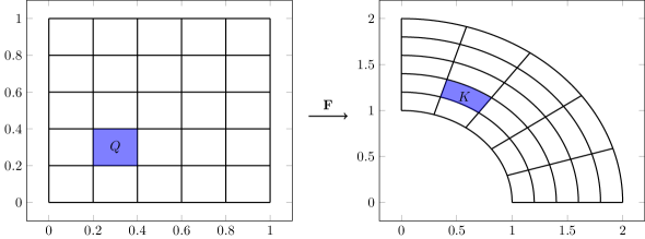
Figure 1: Parametric mesh and the mesh of physical domain $\Omega$.

A mesh on $\Omega$ is provided as the image of the parametric mesh as

$$\mathcal{T}_{h}=\{K=\mathbf{F}(Q)\mid Q\in\widehat{\mathcal{T}}_{h}\}.$$ (51)

Under Assumption VII, we define

$$V_{h}=\mbox{span}\{\mathbf{N}_{\mathbf{i},\mathbf{k}}(\mathbf{x})=\widehat{\mathbf{N}}_{\mathbf{i},\mathbf{k}}\circ\mathbf{F}^{-1}(\mathbf{x})\mid\mathbf{i}\in\mathbf{I}\},$$ (52)

where $h$ is the mesh size $h=\max\{h_{Q}=\mbox{diam}(Q)\mid Q\in\widehat{\mathcal{T}}_{h}\}$. Furthermore, we define

$$h_{K}=\|\nabla\mathbf{F}\|_{L^{\infty}(Q)}h_{Q}\quad(K\in\mathcal{T}_{h}),$$ (53)

where $Q=\mathbf{F}^{-1}(K)$. For the NURBS mesh, we define the regularity of the family of mesh $\{\mathcal{T}_{h}\}_{h}$ using $\{\widehat{\mathcal{T}}_{h}\}$.

Assumption VIII.

The family of the mesh $\{\mathcal{T}_{h}\}_{h}$ is regular, meaning that there exists a positive constant $\sigma$ such that

$$\dfrac{h_{Q}}{h_{Q,\mathrm{min}}}\leq\sigma\quad\quad\left(Q\in\bigcup_{h}\widehat{\mathcal{T}}_{h}\right),$$ (54)

where $h_{Q,\mathrm{min}}$ represents the length of the smallest edge of hypercube $Q$.

We always assume that Assumptions VI, VII and VIII are satisfied. Now we review some results obtained in earlier studies.

Lemma 3.4 (Trace inequality, Theorem 3.2 of [10]).

Letting $K\in\mathcal{T}_{h}$ and $Q=\mathbf{F}^{-1}(K)$, then

$$\|f\|_{L^{2}(\partial K)}^{2}\leq C\lambda_{Q}\lambda_{K}\left(h_{K}^{-1}\|f\|_{L^{2}(K)}^{2}+h_{K}|f|_{H^{1}(K)}^{2}\right)\quad(f\in H^{1}(K)),$$ (55)

where $\lambda_{Q}$ and $\lambda_{K}$ respectively represent the local shape regularity constants of $Q$ and $K$. They are independent of $h_{K}$.

Lemma 3.5 (Inverse inequality, Theorem 4.2. of [1]).

Letting $l$, $m$ be integers with $0\leq m\leq l$, we have

$$\|v_{h}\|_{H^{l}(K)}\leq C_{\mathrm{shape}}h_{K}^{m-l}\displaystyle\sum_{i=0}^{m}\|\nabla\mathbf{F}\|_{L^{\infty}(\mathbf{F}^{-1}(K))}^{i-m}|v_{h}|_{H^{i}(K)},\quad(K\in\mathcal{T}_{h},v_{h}\in V_{h}).$$ (56)

Especially, we have

$$|v_{h}|_{H^{1}(K)}\leq\|v_{h}\|_{H^{1}(K)}\leq C_{\mathrm{shape}}h_{K}^{-1}\|v_{h}\|_{L^{2}(K)}\quad(K\in\mathcal{T}_{h},v_{h}\in V_{h}).$$ (57)

Lemma 3.6 (Quasi-interpolation error estimate, Corollary 4.21 of [4]).

Let the projection $\Pi_{V_{h}}:L^{2}(\Omega)\to V_{h}$ be

$$\Pi_{V_{h}}f=\dfrac{\Pi_{\mathbf{k},\bm{\Xi}}(W(f\circ\mathbf{F}))}{W}\circ\mathbf{F}^{-1}\quad(f\in L^{2}(\Omega)).$$ (58)

Furthermore, letting $s$ be an integer, $l=\min\{k_{1}+1,\cdots,k_{d}+1,s\}$ and $0\leq m\leq l$, then there exists a positive constant $C$ such that

$$\|v-\Pi_{V_{h}}v\|_{H^{m}(K)}\leq Ch_{\widetilde{K}}^{l-m}\|v\|_{H^{\ell}(\widetilde{K})}\quad(K\in\mathcal{T}_{h},v\in H^{s}(\Omega)),$$ (59)

where $\widetilde{K}=\mathbf{F}(\widetilde{Q})$ for $Q=\mathbf{F}^{-1}(K)$ and

$$\widetilde{Q}=\bigcup\left\{\operatorname{supp}\widehat{\mathbf{N}}_{\mathbf{i},\mathbf{k}}:\widehat{\mathbf{N}}_{\mathbf{i},\mathbf{k}}|_{Q}\not\equiv 0\right\}.$$ (60)

In summary, Assumptions II – IV are satisfied under Assumptions VI – VIII.

4 Proof of Theorem 1 and 2

This section is devoted to the proof of theorems for the “elliptic part” $a_{\varepsilon,h}$. We start with the following auxiliary lemma: the estimate (62) itself is well known (see for instance [16, Lemma 2.1]); the estimate (61) is apparently unfamiliar.

Lemma 4.1.

There exists a positive constant $C$ such that

$$\sum_{E\in\mathcal{E}_{h}^{e}}h_{E}\|n\cdot\mu\nabla v\|_{L^{2}(E)}^{2}\leq C\left(|v|_{H^{1}(\Omega)}^{2}+\sum_{K\in\mathcal{T}_{h}}h_{K}^{2}|v|_{H^{2}(K)}^{2}\right)\quad(v\in V).$$ (61)

Particularly, there exists a positive constant $C_{I}$ such that

$$\sum_{E\in\mathcal{E}_{h}^{e}}h_{E}\|n\cdot\mu\nabla v_{h}\|_{L^{2}(E)}^{2}\leq C_{I}|v_{h}|_{H^{1}(\Omega)}^{2}\quad(v_{h}\in V_{h}).$$ (62)

Proof.

Because $\mu\in\mathbb{R}^{d\times d}$ is symmetric, we have

$$\sup_{\xi\in\mathbb{R}^{d}}\dfrac{|\mu\xi|}{|\xi|}=\sup_{\xi\in\mathbb{R}^{d}}\dfrac{\mu\xi\cdot\xi}{|\xi|^{2}}\leq\mu_{1}.$$ (63)

This result implies $|n\cdot\mu\nabla v|\leq\mu_{1}|\nabla v|$. Therefore

$$\|n\cdot\mu\nabla v\|_{L^{2}(E)}^{2}\leq\mu_{1}^{2}\displaystyle\sum_{i=1}^{d}\left\|\operatorname{Tr}\left(\dfrac{\partial v}{\partial x_{i}}\right)\right\|_{L^{2}(E)}^{2}$$ (64)

for all $E\in\mathcal{E}_{h}^{e}$. Here Assumption IV (i) yields

$$\mu_{1}^{2}\displaystyle\sum_{i=1}^{d}\left\|\operatorname{Tr}\left(\dfrac{\partial v}{\partial x_{i}}\right)\right\|_{L^{2}(E)}^{2}\leq C_{\mathrm{Tr}}\mu_{1}^{2}h_{E}^{-1}(|v|_{H^{1}(K_{E})}^{2}+h_{K_{E}}^{2}|v|_{H^{2}(K_{E})}^{2})\quad(v\in V,~{}E\in\mathcal{E}_{h}^{e}),$$ (65)

which implies (61) with $C=C_{\mathrm{Tr}}\mu_{1}^{2}$. Furthermore, using equation (16) leads to the following:

$$\|n\cdot\mu\nabla v_{h}\|_{L^{2}(E)}^{2}\leq\mu_{1}^{2}\displaystyle\sum_{i=1}^{d}\left\|\operatorname{Tr}\left(\dfrac{\partial v_{h}}{\partial x_{i}}\right)\right\|_{L^{2}(E)}^{2}\leq C^{*}\mu_{1}^{2}h_{E}^{-1}|v_{h}|_{H^{1}(K_{E})}^{2}\quad(v_{h}\in V_{h},~{}E\in\mathcal{E}_{h}^{e}).$$

Then we have the estimate (62) with $C_{I}=C^{*}\mu_{1}^{2}$. ∎

Next we can state the following proofs.

Proof of Theorem 1.

First, the Cauchy–Schwarz inequality gives

$$a_{\varepsilon,h}(t;w,v_{h}) \leq M\|w\|_{H^{1}(\Omega)}\|v_{h}\|_{H^{1}(\Omega)}+\left(\displaystyle\sum_{E\in\mathcal{E}_{h}^{e}}h_{E}\|n\cdot\mu\nabla w\|_{L^{2}(E)}^{2}\right)^{1/2}\left(\sum_{E\in\mathcal{E}_{h}^{e}}h_{E}^{-1}\|v_{h}\|_{L^{2}(E)}^{2}\right)^{1/2}$$

$$\quad+\left(\displaystyle\sum_{E\in\mathcal{E}_{h}^{e}}h_{E}\|n\cdot\mu\nabla v_{h}\|_{L^{2}(E)}^{2}\right)^{1/2}\left(\sum_{E\in\mathcal{E}_{h}^{e}}h_{E}^{-1}\|w\|_{L^{2}(E)}^{2}\right)^{1/2}+C\|w\|_{L^{2}(\Gamma)}\|v_{h}\|_{L^{2}(\Gamma)}$$

$$\qquad+\varepsilon\left(\displaystyle\sum_{E\in\mathcal{E}_{h}^{e}}h_{E}^{-1}\|w\|_{L^{2}(E)}^{2}\right)^{1/2}\left(\displaystyle\sum_{E\in\mathcal{E}_{h}^{e}}h_{E}^{-1}\|v_{h}\|_{L^{2}(E)}^{2}\right)^{1/2}$$

for all $w\in V$, $v_{h}\in V_{h}$ and $t\in J$. By applying the (standard) trace inequality and Lemma 4.1, we have

$$a_{\varepsilon,h}(t;w,v_{h})\leq C\|w\|_{V}\|v_{h}\|_{V_{h}}\quad(w\in V,~{}v_{h}\in V_{h},~{}t\in J).$$ (66)

Moreover, the definition of norm $\|\cdot\|_{V}$ and $\|\cdot\|_{V_{h}}$ yields that there exists a positive constant $\widehat{M}$ such that

$$a_{\varepsilon,h}(t;w_{h},v_{h})\leq C\|w_{h}\|_{V}\|v_{h}\|_{V_{h}}\leq\widehat{M}\|w_{h}\|_{V_{h}}\|v_{h}\|_{V_{h}}\quad(w_{h},v_{h}\in V_{h},~{}t\in J),$$ (67)

which is the desired inequality. ∎

Proof of Theorem 2.

Fix $v_{h}\in V_{h}$ and $t\in J$ arbitrarily. First, we mention that $V_{h}\not\subset H^{1}_{0}(\Omega)$. Therefore

$$a(t;v_{h},v_{h})\geq\alpha\|v_{h}\|_{H^{1}(\Omega)}^{2}+\dfrac{1}{2}(b\cdot nv_{h},v_{h})_{L^{2}(\Gamma_{\mathrm{in}})},$$ (68)

and $(b\cdot nv_{h},v_{h})_{\Gamma_{\mathrm{in}}}<0$. Now we have the following:

$$a_{\varepsilon,h}(t;v_{h},v_{h}) \geq\alpha\|v_{h}\|_{H^{1}(\Omega)}^{2}+\dfrac{1}{2}(b\cdot nv_{h},v_{h})_{L^{2}(\Gamma_{\mathrm{in}})}-2\displaystyle\sum_{E\in\mathcal{E}_{h}^{e}}(n\cdot\mu\nabla v_{h},v_{h})_{L^{2}(E)}$$

$$\quad-(b\cdot nv_{h},v_{h})_{L^{2}(\Gamma_{\mathrm{in}})}+\varepsilon\displaystyle\sum_{E\in\mathcal{E}_{h}^{e}}h_{E}^{-1}\|v_{h}\|_{L^{2}(E)}^{2}$$

$$\geq\alpha\|v_{h}\|_{H^{1}(\Omega)}^{2}-\dfrac{1}{2}(b\cdot nv_{h},v_{h})_{L^{2}(\Gamma_{\mathrm{in}})}+\varepsilon\displaystyle\sum_{E\in\mathcal{E}_{h}^{e}}h_{E}^{-1}\|v_{h}\|_{L^{2}(E)}^{2}$$

$$\quad-2\left(\sum_{E\in\mathcal{E}_{h}^{e}}h_{E}\|n\cdot\mu\nabla v_{h}\|_{L^{2}(E)}^{2}\right)^{1/2}\left(\sum_{E\in\mathcal{E}_{h}^{e}}h_{E}^{-1}\|v_{h}\|_{L^{2}(E)}^{2}\right)^{1/2}.$$

Recalling $-(b\cdot nv_{h},v_{h})_{L^{2}(\Gamma_{\mathrm{in}})}>0$ and Lemma 4.1, then we have

$$a_{\varepsilon,h}(t;v_{h},v_{h})\geq\alpha\|v_{h}\|_{H^{1}(\Omega)}^{2}+\varepsilon\sum_{E\in\mathcal{E}_{h}^{e}}h_{E}^{-1}\|v_{h}\|_{L^{2}(E)}^{2}-2C_{I}^{1/2}|v_{h}|_{H^{1}(\Omega)}\left(\sum_{E\in\mathcal{E}_{h}^{e}}h_{E}^{-1}\|v_{h}\|_{L^{2}(E)}^{2}\right)^{1/2}.$$

Here we apply Young’s inequality to obtain

$$2C_{I}^{1/2}|v_{h}|_{H^{1}(\Omega)}\left(\displaystyle\sum_{E\in\mathcal{E}_{h}^{e}}h_{E}^{-1}\|v_{h}\|_{L^{2}(E)}^{2}\right)^{1/2}\leq\dfrac{\alpha}{2}|v_{h}|_{H^{1}(\Omega)}^{2}+2\alpha C_{I}\sum_{E\in\mathcal{E}_{h}^{e}}h_{E}^{-1}\|v_{h}\|_{L^{2}(E)}^{2}.$$ (69)

Then we have

$$a_{\varepsilon,h}(t;v_{h},v_{h})\geq\dfrac{\alpha}{2}\|v_{h}\|_{H^{1}(\Omega)}^{2}+(\varepsilon-2\alpha C_{I})\sum_{E\in\mathcal{E}_{h}^{e}}h_{E}^{-1}\|v_{h}\|_{L^{2}(E)}^{2}.$$ (70)

Letting $\widehat{\alpha}=\min\{\dfrac{\alpha}{2},\varepsilon-2\alpha C_{I}\}$ yields the desired conclusion. ∎

5 Proof of Theorem 3 and 4

This section presents that $B_{\varepsilon,h}$ is continuous and satisfies the inf-sup condition. First, we show Theorem 3.

Proof of Theorem 3.

Recalling that every $z\in X_{V}$ and $z_{h}\in X_{h}\subset C^{0}(\overline{J};V_{h})$ satisfy $z(t)\in V$, $z_{h}(t)\in V_{h}$ for any $t\in J$, we can apply Theorem 1 to obtain

$$B_{\varepsilon,h}(z,\mathbf{y}_{h}) =\int_{J}((\partial_{t}z,y_{h})_{L^{2}(\Omega)}+a_{\varepsilon,h}(t;z,y_{h}))~{}dt+(z(0),\widetilde{y}_{h})_{L^{2}(\Omega)}$$

$$\leq\int_{J}(\|\partial_{t}z\|_{V_{h}^{\prime}}\|y_{h}\|_{V_{h}}+C\|z\|_{V}\|y_{h}\|_{V_{h}})~{}dt+\|z(0)\|_{L^{2}(\Omega)}\|\widetilde{y}_{h}\|_{L^{2}(\Omega)}$$

$$\leq C\|z\|_{X_{V}}\|\mathbf{y}_{h}\|_{Y_{h}}\quad(z\in X_{V},\ \mathbf{y}_{h}=(y_{h},\widetilde{y}_{h})\in Y_{h}),$$

which is the first desired estimate. Moreover, $\|z_{h}\|_{X_{V}}\leq C\|z_{h}\|_{X_{h}}$ leads to the second inequality. ∎

Stating the proof of Theorem 4 requires an auxiliary operator $\mathcal{A}_{\varepsilon,h}(t):V_{h}\to V_{h}$ defined by setting

$$(\mathcal{A}_{\varepsilon,h}(t)w_{h},v_{h})_{L^{2}(\Omega)}=a_{\varepsilon,h}(t;w_{h},v_{h})\quad(w_{h},v_{h}\in V_{h},\ t\in J).$$ (71)

We recall that the bilinear form $a_{\varepsilon,h}(t;\cdot,\cdot):V_{h}\times V_{h}\to\mathbb{R}$ is continuous and coercive. Therefore, the Lax–Milgram theorem shows that the operator $\mathcal{A}_{\varepsilon,h}(t)$ is invertible for $t\in J$. Now we have the following lemma.

Lemma 5.1.

Operator $\mathcal{A}_{\varepsilon,h}(t)^{-1}:V_{h}\to V_{h}$ satisfies

$$\|\mathcal{A}_{\varepsilon,h}(t)^{-1}v_{h}\|_{V_{h}} \leq\widehat{\alpha}^{-1}\|v_{h}\|_{V_{h}^{\prime}},$$ (72)

$$(v_{h},\mathcal{A}_{\varepsilon,h}(t)^{-1}v_{h})_{L^{2}(\Omega)} \geq\widehat{\alpha}\widehat{M}^{-2}\|v_{h}\|_{V_{h}^{\prime}}^{2}$$ (73)

for $v_{h}\in V_{h}$ and $t\in J$.

Proof.

First, we have

$$\widehat{\alpha}\|\mathcal{A}_{\varepsilon,h}(t)^{-1}v_{h}\|^{2}_{V_{h}} \leq(\mathcal{A}_{\varepsilon,h}(t)(\mathcal{A}_{\varepsilon,h}(t)^{-1}v_{h}),\mathcal{A}_{\varepsilon,h}(t)^{-1}v_{h})_{L^{2}(\Omega)}$$

$$=(v_{h},\mathcal{A}_{\varepsilon,h}(t)^{-1}v_{h})_{L^{2}(\Omega)}\leq\|v_{h}\|_{V_{h}^{\prime}}\|\mathcal{A}_{\varepsilon,h}(t)^{-1}v_{h}\|_{V_{h}}$$

for all $v_{h}\in V_{h}$. Therefore we have

$$\|\mathcal{A}_{\varepsilon,h}(t)^{-1}v_{h}\|_{V_{h}}\leq\widehat{\alpha}^{-1}\|v_{h}\|_{V_{h}^{\prime}}\quad(v_{h}\in V_{h},\ t\in J).$$ (74)

Next, it is noteworthy that the constant $\widehat{M}$ satisfies

$$\sup_{0\neq w_{h}\in V_{h}}\dfrac{\|\mathcal{A}_{\varepsilon,h}(t)w_{h}\|_{V_{h}^{\prime}}}{\|w_{h}\|_{V_{h}}}=\sup_{0\neq w_{h}\in V_{h}}\sup_{0\neq v_{h}\in V_{h}}\dfrac{(\mathcal{A}_{\varepsilon,h}(t)w_{h},v_{h})_{L^{2}(\Omega)}}{\|w_{h}\|_{V_{h}}\|v_{h}\|_{V_{h}}}\leq\widehat{M}.$$

Therefore,

$$\|v_{h}\|_{V_{h}^{\prime}}=\|\mathcal{A}_{\varepsilon,h}(t)(\mathcal{A}_{\varepsilon,h}(t)^{-1}v_{h})\|_{V_{h}^{\prime}}\leq\widehat{M}\|\mathcal{A}_{\varepsilon,h}(t)^{-1}v_{h}\|_{V_{h}}$$ (75)

for all $v_{h}\in V_{h}$. This yields

$$(v_{h},\mathcal{A}_{\varepsilon,h}(t)^{-1}v_{h})_{L^{2}(\Omega)} =(\mathcal{A}_{\varepsilon,h}(t)(\mathcal{A}_{\varepsilon,h}(t)^{-1}v_{h}),\mathcal{A}_{\varepsilon,h}(t)^{-1}v_{h})_{L^{2}(\Omega)}$$

$$\geq\widehat{\alpha}\|\mathcal{A}_{\varepsilon,h}(t)^{-1}v_{h}\|^{2}_{V_{h}}$$

$$\geq\widehat{\alpha}\widehat{M}^{-2}\|v_{h}\|_{V_{h}^{\prime}}^{2}\quad(v_{h}\in V_{h},\ t\in J).$$

∎

We can state the following proof.

Proof of Theorem 4.

After fixing $z_{h}\in X_{h}$ arbitrarily, let $\mathbf{y}_{h}:=(\mathcal{A}_{\varepsilon,h}(t)^{-1}(\partial_{t}z_{h})+\delta z_{h},\delta z_{h}(0))\in Y_{h}$, where $\delta:=\widehat{\alpha}^{-4}\widehat{M}^{4}$. Then we have

$$\|\mathbf{y}_{h}\|_{Y_{h}}^{2} =\displaystyle\int_{J}\|\mathcal{A}_{\varepsilon}(t)^{-1}(\partial_{t}z_{h})+\delta z_{h}\|_{V_{h}}^{2}~{}dt+\|\delta z_{h}(0)\|_{L^{2}(\Omega)}^{2}$$

$$\leq\max\{\widehat{\alpha}^{-1},\delta\}\displaystyle\int_{J}(\partial_{t}z_{h}\|_{V_{h}^{\prime}}^{2}+\|z_{h}\|_{V_{h}}^{2})~{}dt+\delta\|z_{h}(0)\|_{L^{2}(\Omega)}^{2}\leq\max\{\widehat{\alpha}^{-1},\delta\}\|z_{h}\|_{X_{h}}^{2},$$

and

$$B_{\varepsilon,h}(z_{h},\mathbf{y}_{h}) =\displaystyle\int_{J}\left((\partial_{t}z_{h},\mathcal{A}_{\varepsilon,h}(t)^{-1}(\partial_{t}z_{h})+\delta z_{h})_{L^{2}(\Omega)}+a_{\varepsilon,h}(t;z_{h},\mathcal{A}_{\varepsilon,h}(t)^{-1}(\partial_{t}z_{h})+\delta z_{h})\right)~{}dt$$

$$\qquad+(z_{h}(0),\delta z_{h}(0))_{L^{2}(\Omega)}$$

$$\geq\displaystyle\int_{J}(\widehat{\alpha}\widehat{M}^{-2}\|\partial_{t}z_{h}\|_{V_{h}^{\prime}}^{2}-\widehat{\alpha}^{-1}\widehat{M}\|z_{h}\|_{V_{h}}\|\partial_{t}z_{h}\|_{V_{h}^{\prime}}+\delta\widehat{\alpha}\|z_{h}\|_{V_{h}}^{2})~{}dt$$

$$\qquad+\delta/2(\|z_{h}(T)\|_{L^{2}(\Omega)}^{2}-\|z_{h}(0)\|_{L^{2}(\Omega)}^{2})+\delta\|z_{h}(0)\|_{L^{2}(\Omega)}^{2}$$

$$\geq\displaystyle\int_{J}(\widehat{\alpha}\widehat{M}^{-2}\|\partial_{t}z_{h}\|_{V_{h}^{\prime}}^{2}-\widehat{\alpha}^{-1}\widehat{M}\|z_{h}\|_{V_{h}}\|\partial_{t}z_{h}\|_{V_{h}^{\prime}}+\delta\widehat{\alpha}\|z_{h}\|_{V_{h}}^{2})~{}dt$$

$$\qquad+\delta/2\|z_{h}(0)\|_{L^{2}(\Omega)}^{2}$$

$$\geq\displaystyle\int_{J}\left(\widehat{\alpha}\widehat{M}^{-2}/2\|\partial_{t}z_{h}\|_{V_{h}^{\prime}}^{2}+(\delta\widehat{\alpha}-\widehat{\alpha}^{-3}\widehat{M}^{4}/2)\|z_{h}\|_{V_{h}}^{2}\right)~{}dt+\delta/2\|z_{h}(0)\|_{L^{2}(\Omega)}^{2}$$

$$\geq 1/2\min\{\widehat{\alpha}\widehat{M}^{-2},\widehat{\alpha}^{-3}\widehat{M}^{4},\widehat{\alpha}^{-4}\widehat{M}^{4}\}\left(\displaystyle\int_{J}(\|\partial_{t}z_{h}\|_{V_{h}^{\prime}}^{2}+\|z_{h}\|_{V_{h}}^{2})~{}dt+\|z_{h}(0)\|_{L^{2}(\Omega)}^{2}\right)$$

$$=1/2\min\{\widehat{\alpha}\widehat{M}^{-2},\widehat{\alpha}^{-3}\widehat{M}^{4},\widehat{\alpha}^{-4}\widehat{M}^{4}\}\|z_{h}\|_{X_{h}}^{2}.$$

The two inequalities above imply that

$$a_{\varepsilon,h}(z_{h},\mathbf{y}_{h})\geq\beta\|z_{h}\|_{X_{h}}\|\mathbf{y}_{h}\|_{Y_{h}},$$ (76)

where $\beta=1/2\min\{\widehat{\alpha}\widehat{M}^{-2},\widehat{\alpha}^{-3}\widehat{M}^{4},\widehat{\alpha}^{-4}\widehat{M}^{4}\}\min\{\widehat{\alpha}^{1/2},\widehat{\alpha}^{2}\widehat{M}^{-2}\}$. Therefore we have

$$\inf_{0\neq z_{h}\in X_{h}}\sup_{0\neq\mathbf{y}_{h}\in Y_{h}}\dfrac{a_{\varepsilon,h}(z_{h},\mathbf{y}_{h})}{\|z_{h}\|_{X_{h}}\|\mathbf{y}_{h}\|_{Y_{h}}}\geq\beta$$ (77)

The inf-sup condition follows.

∎

6 Proof of Theorem 9

We need the following lemma, which is a direct consequence of Assumptions II and IV (see [16, Lemma 2.3] for example).

Lemma 6.1.

Letting $l$ be an integer with $2\leq l\leq k+1$, then there exist two positive constants $C_{1}$ and $C_{2}$ such that

$$\|v-\Pi_{h}v\|_{V_{h}}\leq C_{1}h^{l-1}\|v\|_{H^{l}(\Omega)},$$ (78a)

$$\|v-\Pi_{h}v\|_{V}\leq C_{2}h^{l-1}\|v\|_{H^{l}(\Omega)}$$ (78b)

for all $v\in H^{l}(\Omega)$.

We recall that the exact solution is $u$ assumed to belong to $X_{l,m}=H^{1}(J;H^{l}(\Omega),H^{m}(\Omega))$ for $2\leq l,m\leq k+1$. Then $\Pi_{h}$ defines a projection from $X_{l,m}$ to $X_{h}$. We designate by $\Pi_{h}$ again, i.e.,

$$(\Pi_{h}u)(t)=\Pi_{h}u(t)\quad(t\in\overline{J}),\qquad\partial_{t}(\Pi_{h}u)(t)=\Pi_{h}(\partial_{t}u(t))\quad(t\in J).$$

The estimate in Theorem 8 is valid for $z_{h}=\Pi_{h}u$, which gives the following proof.

Proof of Theorem 9.

It is readily apparent that $X_{\ell,m}\subset X_{V}$. Therefore Theorem 8 implies

$$\|u-u_{\varepsilon,h}\|_{X_{h}}^{2} \leq\displaystyle\inf_{z_{h}\in X_{h}}C\|u-z_{h}\|_{X_{V}}^{2}$$

$$\leq\|u-\Pi_{h}u\|_{X_{V}}^{2}$$

$$=\displaystyle\int_{J}\left(\|u-\Pi_{h}u\|_{V}^{2}+\|\partial_{t}(u-\Pi_{h}u)\|_{V_{h}^{\prime}}^{2}\right)dt+\|u(0)-\Pi_{h}u(0)\|_{L^{2}(\Omega)}^{2}.$$

We can estimate that

$$\|u-\Pi_{h}u\|_{V}^{2}\leq Ch^{2(l-1)}\|u\|_{H^{l}(\Omega)},$$ (79)

$$\|\partial_{t}(u-\Pi_{h}u)|_{V_{h}^{\prime}}^{2}\leq\|\partial_{t}u-\Pi_{h}(\partial_{t}u)\|_{L^{2}(\Omega)}\leq Ch^{2m}\|\partial_{t}u\|_{H^{m}(\Omega)}.$$ (80)

Moreover, because

$$X_{l,m}=H^{1}(J;H^{l}(\Omega),H^{m}(\Omega))\subset H^{1}(J;H^{j}(\Omega),H^{j}(\Omega))\subset C^{0}(\overline{J};H^{j}(\Omega)),$$ (81)

where $j=\min\{l,m\}$, we have $u(0)\in H^{j}(\Omega)$, and

$$\|u(0)-\Pi_{h}u(0)\|_{L^{2}(\Omega)}^{2}\leq Ch^{2j}\|u(0)\|_{H^{j}(\Omega)}^{2}.$$ (82)

Summing up those estimates, we complete the proof. ∎

7 Full discretization

Let $N\in\mathbb{N}$ be the number of time steps, $\tau=T/N$ and $t_{n}=n\tau$. We now consider the temporal discretization with implicit Euler (backward Euler) method.

(P_ε,h,τ) Find $\{u_{\varepsilon,h,\tau}^{n}\}_{n=0}^{N}\in(V_{h})^{N+1}$ such that

$$\dfrac{1}{\tau}(u_{\varepsilon,h,\tau}^{n}-u_{\varepsilon,h,\tau}^{n-1},v_{h})_{L^{2}(\Omega)}+a_{\varepsilon,h}(t_{n};u_{\varepsilon,h,\tau}^{n},v_{h})=F_{\varepsilon,h}(t_{n};v_{h})\quad(v_{h}\in V_{h}),$$ (83a)

$$(u_{\varepsilon,h,\tau}^{0}-u_{0},\widetilde{v}_{h})_{L^{2}(\Omega)}=0\quad(\widetilde{v}_{h}\in V_{h})$$ (83b)

Clearly, $u_{\varepsilon,h,\tau}^{0}=u_{\varepsilon,h}(0)$, where $u_{\varepsilon,h}\in X_{h}$ represents the solution of (P_ε,h).

Lemma 7.1.

The problem (P_ε,h,τ) has a unique solution $\{u_{\varepsilon,h,\tau}^{n}\}_{n=0}^{N}\in(V_{h})^{N+1}$.

Proof.

It is readily apparent that $u_{\varepsilon,h,\tau}^{0}\in V_{h}$. We take the basis functions $\{\phi_{i}\}_{i=1}^{N}$ of $V_{h}$, where $N=\operatorname{dim}V_{h}$, and

$$u_{\varepsilon,h,\tau}^{n}:=\displaystyle\sum_{i=1}^{N}u_{\varepsilon,h,\tau,i}^{n}\phi_{i}.$$ (84)

Then, the equation (83a) implies the following for $n=1,\cdots,N$,

$$\left(\mathbf{M}+\Delta t\mathbf{A}^{n}\right)\mathbf{u}_{\varepsilon,h,\tau}^{n}=\mathbf{M}\mathbf{u}_{\varepsilon,h,\tau}^{n-1}+\Delta t\mathbf{F}^{n},$$ (85)

where $(\mathbf{M})_{ij}:=(\phi_{i},\phi_{j})_{L^{2}(\Omega)}$, $(\mathbf{A}^{n})_{ij}:=a_{\varepsilon,h}(t_{n};\phi_{i},\phi_{j})$, $(\mathbf{F}^{n})_{i}:=F_{\varepsilon,h}(t_{n};\phi_{i})$ and $\mathbf{u}_{\varepsilon,h,\tau}^{n}:=(u_{\varepsilon,h,\tau,1}^{n},\cdots,u_{\varepsilon,h,\tau,N})^{\operatorname{T}}$. Theorem 2 gives $\mathbf{M}+\Delta t\mathbf{A}^{n}$ as a positive definite matrix. Therefore, there exists a unique $u_{\varepsilon,h,\tau}^{n}$ for any $u_{\varepsilon,h,\tau}^{n-1}$. ∎

Let

$$\mathcal{S}_{\tau}=\left\{w_{h}:[0,T]\to V_{h}\mid\begin{array}[]{c}\mbox{ For all }n=1,\cdots,N,\mbox{ there exists }v_{h}\in V_{h}\\ \mbox{ such that }w_{h}|_{(t_{n-1},t_{n}]}=v_{h},\mbox{ and }w_{h}(0)\in V_{h}\end{array}\right\},$$ (86)

and $v_{h,\tau}(t_{n}^{+})=\lim_{t\to t_{n}+0}v_{h,\tau}(t)$ for $v_{h,\tau}\in\mathcal{S}_{\tau}$. It is noteworthy that $\mathcal{S}_{\tau}\subset L^{2}\left(J;V_{h}\right)$. The solution of (P_ε,h,τ) can be extended to an element of $\mathcal{S}_{\tau}$ as

$$u_{\varepsilon,h,\tau}(t)=\left\{\begin{array}[]{ll}u_{0}&\mbox{if }t=0,\\ u_{\varepsilon,h,\tau}^{n+1}&\mbox{if }t\in(t_{n},t_{n+1}]\quad(n=0,\cdots,N-1).\end{array}\right.$$ (87)

One can show that $u_{\varepsilon,h,\tau}\in\mathcal{S}_{\tau}$ satisfies the following estimate.

Lemma 7.2.

Assuming that $u_{\varepsilon,h}\in C^{2}\left(\overline{J};V_{h}\right)$, then let $\Pi_{\tau}u_{\varepsilon,h}\in\mathcal{S}_{\tau}$ be

$$\Pi_{\tau}u_{\varepsilon,h}(t)=\left\{\begin{array}[]{ll}u_{0}&\mbox{if }t=0,\\ u_{\varepsilon,h}(t_{n+1})&\mbox{if }t\in(t_{n},t_{n+1}]\quad(n=0,\cdots,N-1)\end{array}\right.$$ (88)

and $\rho=u_{\varepsilon,h,\tau}-\Pi_{\tau}u_{\varepsilon,h}\in\mathcal{S}_{\tau}$, where $u_{\varepsilon,h}\in X_{h}$ is the solution of (P_ε,h). Based on the relations presented above,

$$\displaystyle\max_{n=0,\cdots,N-1}\|\rho(t_{n}^{+})\|_{L^{2}(\Omega)}\leq\sqrt{\dfrac{T}{8\widehat{\alpha}}}\tau\|\partial_{t}^{2}u_{\varepsilon,h}\|_{L^{\infty}(J;L^{2}(\Omega))},$$ (89a)

$$\|\rho\|_{L^{2}(J;V_{h})}\leq\dfrac{\sqrt{T}}{2\widehat{\alpha}}\tau\|\partial_{t}^{2}u_{\varepsilon,h}\|_{L^{\infty}(J;L^{2}(\Omega))}.$$ (89b)

Proof.

Clearly, $\rho(t_{0})=0$. In fact, $u_{\varepsilon,h}\in C^{2}\left(\overline{J};V_{h}\right)$ and the definition of $u_{\varepsilon,h,\tau}$ yield

$$u_{\varepsilon,h,\tau}^{n+1}=u_{\varepsilon,h,\tau}(t_{n}^{+})=u_{\varepsilon,h,\tau}(t_{n+1}),$$ (90a)

$$u_{\varepsilon,h}(t_{n+1})=\Pi_{\tau}u_{\varepsilon,h}(t_{n}^{+})=\Pi_{\tau}u_{\varepsilon,h}(t_{n+1}).$$ (90b)

Using (90a), equation (83a) is written, equivalently, as

$$(u_{\varepsilon,h,\tau}(t_{n}^{+})-u_{\varepsilon,h,\tau}(t_{n}),v_{h,\tau}(t_{n}^{+}))_{L^{2}(\Omega)}+\tau a_{\varepsilon,h}(t_{n+1};u_{\varepsilon,h,\tau}(t_{n}^{+}),v_{h,\tau}(t_{n}^{+}))\\ =\tau F_{\varepsilon,h}(t_{n+1};v_{h,\tau}(t_{n}^{+}))\quad(v_{h,\tau}\in\mathcal{S}_{\tau}).$$ (91)

Furthermore, equations (90b) and (19) yield

$$(\Pi_{\tau}u_{\varepsilon,h}(t_{n}^{+})-\Pi_{\tau}u_{\varepsilon,h}(t_{n})+\tau^{2}/2\partial_{t}^{2}u_{\varepsilon,h}(c_{n}),v_{h,\tau}(t_{n}^{+}))_{L^{2}(\Omega)}+\tau a_{\varepsilon,h}(t_{n+1};\Pi_{\tau}u_{\varepsilon,h}(t_{n}^{+}),v_{h,\tau}(t_{n}^{+}))\\ =\tau F_{\varepsilon,h}(t_{n+1};v_{h,\tau}(t_{n}^{+}))\quad(v_{h,\tau}\in\mathcal{S}_{\tau})$$ (92)

for some $c_{n}\in(t_{n},t_{n+1}]$. By the two equations presented above, setting $v_{h,\tau}=\rho\in\mathcal{S}_{\tau}$ leads to

$$(\rho(t_{n}^{+})-\rho(t_{n}),\rho(t_{n}^{+}))_{L^{2}(\Omega)}-\tau^{2}/2(\partial_{t}^{2}u_{\varepsilon,h}(c_{n}),\rho(t_{n}^{+}))_{L^{2}(\Omega)}+\tau a_{\varepsilon,h}(t_{n+1};\rho,\rho)=0.$$ (93)

Now we can estimate

$$(\rho(t_{n}^{+})-\rho(t_{n}),\rho(t_{n}^{+}))_{L^{2}(\Omega)} =\dfrac{1}{2}(\|\rho(t_{n}^{+})-\rho(t_{n})\|_{L^{2}(\Omega)}^{2}+\|\rho(t_{n}^{+})\|_{L^{2}(\Omega)}^{2}-\|\rho(t_{n})\|_{L^{2}(\Omega)}^{2})$$

$$\geq\dfrac{1}{2}(\|\rho(t_{n}^{+})\|_{L^{2}(\Omega)}^{2}-\|\rho(t_{n})\|_{L^{2}(\Omega)}^{2}),$$

$$-\tau^{2}/2(\partial_{t}^{2}u_{\varepsilon,h}(c_{n}),\rho(t_{n}^{+}))_{L^{2}(\Omega)} \geq-\tau^{3/2}/2\|\partial_{t}^{2}u_{\varepsilon,h}\|_{L^{\infty}(J;L^{2}(\Omega))}\|\rho\|_{L^{2}(t_{n},t_{n+1};V_{h})}$$

$$\geq-\left(\dfrac{\tau^{3}}{16q}\|\partial_{t}^{2}u_{\varepsilon,h}\|_{L^{\infty}(J;L^{2}(\Omega))}^{2}+q\|\rho\|_{L^{2}(t_{n},t_{n+1};V_{h})}^{2}\right)$$

for any $$q\in\mathbb{R}$$, and

$$\tau a_{\varepsilon,h}(t_{n+1};\rho,\rho)\geq\widehat{\alpha}\|\rho\|_{L^{2}(t_{n},t_{n+1};V_{h})}.$$ (94)

Therefore, letting $q=\widehat{\alpha}$ yields

$$\|\rho(t_{n}^{+})\|_{L^{2}(\Omega)}^{2} \leq\|\rho(t_{n-1}^{+})\|_{L^{2}(\Omega)}^{2}+\dfrac{\tau^{3}}{8\widehat{\alpha}}\|\partial_{t}^{2}u_{\varepsilon,h}\|_{L^{\infty}(J;L^{2}(\Omega))}^{2}$$

$$\leq\|\rho(t_{0})\|_{L^{2}(\Omega)}^{2}+\dfrac{\tau^{3}(n+1)}{8\widehat{\alpha}}\|\partial_{t}^{2}u_{\varepsilon,h}\|_{L^{\infty}(J;L^{2}(\Omega))}^{2}$$

$$\leq\dfrac{T}{8\widehat{\alpha}}\tau^{2}\|\partial_{t}^{2}u_{\varepsilon,h}\|_{L^{\infty}(J;L^{2}(\Omega))}^{2}$$

for all $n=0,\cdots,N=1$. Furthermore, if we set $q=\dfrac{\widehat{\alpha}}{2}$, then we have

$$\widehat{\alpha}\|\rho\|_{L^{2}(t_{n},t_{n+1};V_{h})}^{2}+\|\rho(t_{n}^{+})\|_{L^{2}(\Omega)}^{2}-\|\rho(t_{n})\|_{L^{2}(\Omega)}^{2}\leq\dfrac{\tau^{3}}{4\widehat{\alpha}}\|\partial_{t}^{2}u_{\varepsilon,h}\|_{L^{\infty}(J;L^{2}(\Omega))}^{2}.$$ (95)

Summing this from $n=0$ to $n=N-1$ gives

$$\|\rho\|_{L^{2}(J;V_{h})}^{2} \leq\dfrac{1}{\widehat{\alpha}}\|\rho(t_{0})\|_{L^{2}(\Omega)}^{2}+\dfrac{\tau^{3}N}{4\widehat{\alpha}^{2}}\|\partial_{t}^{2}u_{\varepsilon,h}\|_{L^{\infty}(J;L^{2}(\Omega))}^{2}$$

$$\leq\dfrac{T}{4\widehat{\alpha}^{2}}\tau^{2}\|\partial_{t}^{2}u_{\varepsilon,h}\|_{L^{\infty}(J;L^{2}(\Omega))}^{2}.$$

∎

Theorem 10 (Error estimate).

Let $l,m$ be two integers satisfying $2\leq l,m\leq k+1$. Assuming that $u\in X_{l,m}$ and $u_{\varepsilon,h}\in C^{2}(\overline{J};V_{h})$, then there exists a positive constant $C$ such that

$$\|u-u_{\varepsilon,h,\tau}\|_{L^{2}(J;H^{1}(\Omega))}^{2} \leq C\Biggl{(}\displaystyle\int_{J}(h^{2(l-1)}\|u\|_{H^{l}(\Omega)}^{2}+h^{2m}\|\partial_{t}u\|_{H^{m}(\Omega)}^{2})~{}dt+h^{2j}\|u(0)\|_{H^{j}(\Omega)}^{2}$$

$$\qquad+\tau^{2}\|\partial_{t}u_{\varepsilon,h}\|_{L^{2}(J;H^{1}(\Omega))}^{2}+\dfrac{T}{4\widehat{\alpha}^{2}}\tau^{2}\|\partial_{t}^{2}u_{\varepsilon,h}\|_{L^{\infty}(J;L^{2}(\Omega))}^{2}\Biggr{)},$$

where $j:=\min\{l,m\}$.

Proof.

We have

$$\|u-u_{\varepsilon,h,\tau}\|_{L^{2}(J;H^{1}(\Omega))}^{2}\leq\|u-u_{\varepsilon,h}\|_{X_{h}}^{2}+\|u_{\varepsilon,h}-\Pi_{\tau}u_{\varepsilon,h}\|_{L^{2}(J;H^{1}(\Omega))}^{2}+\|\Pi_{\tau}u_{\varepsilon,h}-u_{\varepsilon,h,\tau}\|_{L^{2}(J;V_{h})}^{2}.$$

Here Theorem 9, Lemma 7.2 and the approximation error estimate for piecewise constant yield the result. ∎

8 Numerical examples

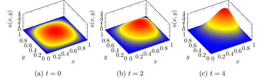
Figure 2: Exact solutions at different time steps.

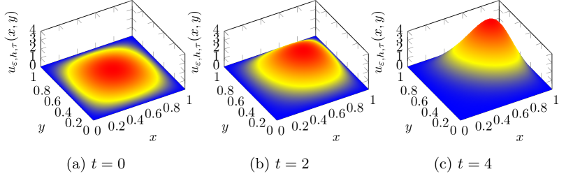
Figure 3: Numerical solutions of the Nitsche method at different time steps by consideration of a uniform mesh with mesh size $h=1/30$.

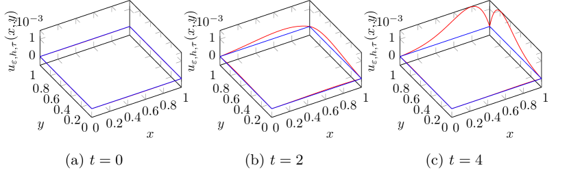
Figure 4: Numerical solutions of the Nitsche method on boundary $\Gamma$, at different time steps by consideration of a uniform mesh with mesh size $h=1/30$.

Our example is given as $\Omega:=(0,1)^{2}$, $J=(0,4)$, and

$$\left\{\begin{array}[]{rll}\partial_{t}u-\Delta u+(1,1)^{\mathrm{T}}\cdot\nabla u+u&=f(\mathbf{x},t)&\mbox{in }\Omega\times J,\\ u&=0&\mbox{on }\Gamma\times J,\\ u(\mathbf{x},0)&=\sin(\pi x)\sin(\pi y)&\mbox{for }\mathbf{x}=(x,y)\in\Omega.\end{array}\right.$$ (96)

That is, we let $\mu(\mathbf{x},t)=I$, $\mathbf{a}(\mathbf{x},t)=(1,1)^{\mathrm{T}}$ and $c(\mathbf{x},t)=1$. One can readily check that this problem has a unique solution for any $f\in L^{2}(J;H^{-1}(\Omega))$. We let

$$f(x,y,t) :=\left((x+y+2t-2t^{2}+2\pi^{2})\sin(\pi x)\sin(\pi y)\right.$$

$$\hskip 28.45274pt\left.+(\pi-2\pi t)\cos(\pi x)\sin(\pi y)+(\pi-2\pi t)\sin(\pi x)\cos(\pi y)\right)e^{(x+y-1)t},$$

Then $f\in L^{2}(J;H^{1}(\Omega))$, and

$$u(x,y,t):=\sin(\pi x)\sin(\pi y)e^{(x+y-1)t}$$ (97)

is the unique solution. In Figure 2, we show the exact solution at different time steps.

We use the $(k,k)$-th degree B-spline basis functions for spatial discretization using the uniform mesh and implicit Euler scheme for temporal discretization, where $k=1,2$: we consider the approximate problem (83a). We let $\tau=O(h^{k})$, where $h$ is the mesh size for uniform mesh. Then we know from Theorem 10 that

$$\|u-u_{\varepsilon,h,\tau}\|_{L^{2}\left(J;H^{1}(\Omega)\right)}\leq Ch^{k}.$$ (98)

As shown in Figure 3, this report describes the numerical solution shape. Then we show the boundary value of the numerical solution in Figure 4. The weak imposition of the Dirichlet boundary condition is actually observed because the boundary value does not vanish.

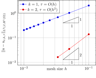
Figure 5: $L^{2}(J;H^{1}(\Omega))$ error on a uniform mesh.

Furthermore, this report describes the error for uniform mesh in Figure 5, which shows that the rate of convergence is approximately equal to $k$, which is expected by the theory.

Acknowledgements.

This study was supported by JST CREST Grant Number JPMJCR15D1 and JSPS KAKENHI Grant Number 15H03635. The first author was also supported by the Program for Leading Graduate Schools, MEXT, Japan.

References

- [1] Y. Bazilevs, L. Beirão da Veiga, J. A. Cottrell, T. J. R. Hughes, and G. Sangalli. Isogeometric analysis: approximation, stability and error estimates for -refined meshes. Math. Models Methods Appl. Sci., 16(7):1031–1090, 2006.
- [2] Y. Bazilevs and T. J. R. Hughes. Weak imposition of Dirichlet boundary conditions in fluid mechanics. Comput. & Fluids, 36(1):12–26, 2007.
- [3] Y. Bazilevs, C. Michler, V. M. Calo, and T. J. R. Hughes. Weak Dirichlet boundary conditions for wall-bounded turbulent flows. Comput. Methods Appl. Mech. Engrg., 196(49-52):4853–4862, 2007.
- [4] L. Beirão da Veiga, A. Buffa, G. Sangalli, and R. Vázquez. Mathematical analysis of variational isogeometric methods. Acta Numer., 23:157–287, 2014.
- [5] S. C. Brenner and L. R. Scott. The Mathematical Theory of Finite Element Methods, volume 15 of Texts in Applied Mathematics. Springer, New York, third edition, 2008.
- [6] G. Choudury and I. Lasiecka. Optimal convergence rates for semidiscrete approximations of parabolic problems with nonsmooth boundary data. Numer. Funct. Anal. Optim., 12(5-6):469–485 (1992), 1991.
- [7] J. A. Cottrell, T. J. R. Hughes, and Y. Bazilevs. Isogeometric Analysis: Toward Integration of CAD and FEA. Wiley, 2009.
- [8] R. Dautray and J. L. Lions. Mathematical analysis and numerical methods for science and technology. Vol. 5. Springer-Verlag, Berlin, 1992. Evolution problems. I, With the collaboration of Michel Artola, Michel Cessenat and Hélène Lanchon, Translated from the French by Alan Craig.
- [9] A. Ern and J. L. Guermond. Theory and practice of finite elements, volume 159 of Applied Mathematical Sciences. Springer-Verlag, New York, 2004.
- [10] J. A. Evans and T. J. R. Hughes. Explicit trace inequalities for isogeometric analysis and parametric hexahedral finite elements. Numer. Math., 123(2):259–290, 2013.
- [11] L. C. Evans. Partial differential equations, volume 19 of Graduate Studies in Mathematics. American Mathematical Society, Providence, RI, second edition, 2010.
- [12] B. Heinrich and B. Jung. Nitsche mortaring for parabolic initial-boundary value problems. Electron. Trans. Numer. Anal., 32:190–209, 2008.
- [13] J. Nitsche. Über ein Variationsprinzip zur Lösung von Dirichlet-Problemen bei Verwendung von Teilr äumen, die keinen Randbedingungen unterworfen sind. Abh. Math. Sem. Univ. Hamburg, 36:9–15, 1971. Collection of articles dedicated to Lothar Collatz on his sixtieth birthday.
- [14] N. Saito. Variational analysis of the discontinuous Galerkin time-stepping method for parabolic equations. arXiv:1710.10543.
- [15] L. L. Schumaker. Spline functions: basic theory. Cambridge Mathematical Library. Cambridge University Press, Cambridge, third edition, 2007.
- [16] V. Thomée. Galerkin finite element methods for parabolic problems. Springer Verlag, Berlin, second edition, 2006.
- [17] J. Wloka. Partial differential equations. Cambridge University Press, Cambridge, 1987. Translated from the German by C. B. Thomas and M. J. Thomas.