Unconventional scaling theory in disorder-driven quantum phase transition

Abstract

We clarify novel forms of scaling functions of conductance, critical conductance distribution and localization length in a disorder-driven quantum phase transition between band insulator and Weyl semimetal phases. Quantum criticality of the phase transition is controlled by a clean-limit fixed point with spatially anisotropic scale invariance. We argue that the anisotropic scale invariance is reflected on unconventional scaling function forms in the quantum phase transition. We verify the proposed scaling function forms in terms of transfer-matrix calculations of conductance and localization length in a tight-binding model.

Scaling theories play a central role in the studies of Anderson localization anderson58 ; wegner76 as well as other disorder-driven quantum phase transitions. Inspired by the finite size scaling theory by the gang of four abrahams79 , scaling theories of localization length mackinnon81 ; pichard81 , and conductance anderson80 ; slevin01prl have been developed and become the core of our current understandings of the localization phenomena. The theories facilitate numerical studies of the phenomena, that establish a rich variety of the universality classes wigner51 ; dyson62a ; dyson62b ; zirnbauer96 ; altland97 . All the Wigner-Dyson universality classes are characterized and distinguished from one another by critical and dynamical exponents, and critical conductance distribution (CCD) shapiro90 ; cohen92 ; slevin97 ; slevin00 . Meanwhile, all of them obey the similar scaling functions;

$$Q(L,m,\Delta_{1},\Delta_{2},\cdots)=F_{Q}(m^{\nu}L,m^{|y_{1}|}\Delta_{1},\cdots).$$ (1)

Here $Q$ is a (properly normalized) dimensionless physical quantity, $L$ is a linear dimension of the system size, $m$ is a relevant scaling variable with its scaling dimension $\nu$, and $\Delta_{j}$ ($j=1,2,\cdots$) is an irrelevant scaling variable with negative scaling dimension $y_{j}$. Naturally one may raise a question by asking “Is there any new disorder-driven quantum phase transition that obeys different forms of scaling functions ?”

In this rapid communication, we answer this question affirmatively, by investigating quantum criticality of a disorder-driven phase transition between band insulator (BI) and Weyl semimetal (WSM) phases. We clarify novel forms of scaling functions of conductance, CCD and localization length such as in Eqs. (5), (10), (11), (12), and (13). The criticality of the BI-WSM transition is controlled by a fixed point in the clean limit that has spatially anisotropic scale invariant property cardy ; yang1 ; carpentier ; yang2 ; jrwang ; roy16arXiv ; luo18 . We show that the anisotropic scale invariance results in unconventional forms of scaling functions for conductance, CCD and localization length in the disorder-driven BI-WSM quantum phase transition. Based on numerical simulations on a lattice model with disorders, we demonstrate the validity of the proposed scaling properties.

Weyl semimetal (WSM) is a class of three-dimensional semimetal that has a band touching point with linear dispersions along all the three directions (‘Weyl node’) murakami07 ; balents11 ; weng15 ; sy-xu15 ; bq-lv15 . The Nielsen-Ninomiya theorem dictates that two band touching points with the linear dispersions must appear in a pair in the first Brillouin zone. When a pair of two Weyl nodes annihilate with each other, the system undergoes a quantum phase transition from WSM to BI phases. The phase transition is described by an effective continuum model with a magnetic dipole in the momentum space yang1 ; yang2 ; roy16arXiv ; luo18 ,

$${\cal H}_{\rm eff} =\int d^{2}{\bm{x}}_{\perp}dz\!\ \psi^{\dagger}({\bm{x}})\Big{\{}iv\big{(}\partial_{x}{\bm{\sigma}}_{x}+\partial_{y}{\bm{\sigma}}_{y}\big{)}$$

$$\ \ \ -\big{(}(-i)^{2}b_{2}\partial^{2}_{z}-m\big{)}{\bm{\sigma}}_{z}\Big{\}}\psi({\bm{x}}),$$ (2)

with ${\bm{x}}_{\perp}\equiv(x,y)$ and ${\bm{x}}\equiv({\bm{x}}_{\perp},z)$. ${\bm{\sigma}}_{\mu}$ ($\mu=x,y,z$) are 2 $\times$ 2 Pauli matrices. For positive $m$ (WSM phase), the electronic system at $E=0$ has a pair of Weyl nodes with the opposite magnetic monopole charges at ${\bm{k}}_{\rm MM}=(0,0,\pm\sqrt{m/b_{2}})$; ‘magnetic dipole’ in the momentum space. For negative $m$ (BI phase), the system has an energy gap at the zero energy. Previously, the stability of the critical point ($m=0$) against the Coulomb interaction yang1 ; yang2 as well as short-ranged disorder yang1 ; roy16arXiv ; luo18 has been studied. Especially, a tree-level renormalization group analysis on the continuum model dictates that the quantum critical point at $m=0$ is robust against any types of short-ranged disorder yang1 ; yang2 ; roy16arXiv ; luo18 ; fradkin86 ; goswami11 ; syzranov15prb ; syzranov15prl . Thus, small but finite disorder is always renormalized to the critical point in the clean limit, as long as the disorder strength is smaller than a certain critical value $\Delta_{c}$ (Fig. 1). Quantum criticality of the disorder-driven BI-WSM quantum phase transition at finite $\Delta<\Delta_{c}$ is controlled by the clean-limit fixed point at $m=\Delta=0$. We dub the fixed point as ‘FP0’ as in Fig. 1.

The gapless theory at $m=\Delta=0$ has a quadratic dispersion along the dipole ($z$) direction, while it has linear dispersions within the perpendicular ($xy$) directions. Thereby, the clean-limit fixed point has the following spatially anisotropic scale invariant property;

$$z^{\prime} =b^{\frac{1}{2}}\!\ z,\ \ {\bm{x}}^{\prime}_{\perp}=b\!\ {\bm{x}}_{\perp},$$ (3)

with time $t^{\prime}=b\!\ t$ and the single-particle energy $E^{\prime}=b^{-1}E$. Hereafter a symbol for the scale change, $b\equiv e^{-dl}<1$, counts how many times we carry out a renormalization. Quantities with and without prime denote those after and before the renormalization, respectively. As we will see below, the anisotropic scaling leads to new forms of scaling functions for the conductance and localization length at the Weyl nodes ($E=0$).

Let us begin with the scaling property of the zero-energy conductance. According to the anisotropic scaling, the density state per volume $\rho(E)$ scales as $\rho^{\prime}(E^{\prime})=b^{-(d-\frac{1}{2}-1)}\rho(E)$ at the fixed point (FP0) yang1 ; roy16arXiv ; luo18 , where $b^{-(d-\frac{1}{2})}$ and $b^{+1}$ come from Eq. (3) and $E^{\prime}=b^{-1}E$, respectively. The diffusion constant along the dipole direction scales as $D^{\prime}_{z}=b^{-(1-1)}D_{z}=D_{z}$, while that along the perpendicular directions scales as $D^{\prime}_{\perp}=b^{-(1-2)}D_{\perp}$ luo18 . Thus, the Einstein relation, $\sigma_{\mu}\equiv e^{2}D_{\mu}\rho$, gives the conductivity scaling at the fixed point in the clean limit as $\sigma^{\prime}_{z}=b^{-d+\frac{3}{2}}\sigma_{z}$ and $\sigma^{\prime}_{\perp}=b^{-d+\frac{5}{2}}\sigma_{\perp}$ respectively luo18 . With $G_{z}\equiv\sigma_{z}L^{d-1}_{\perp}/L_{z}$ and $G_{\perp}\equiv\sigma_{\perp}L^{d-3}_{\perp}L_{z}$, one naturally reaches the following scaling relations of the zero-energy conductances under the renormalization;

$$G^{\prime}_{\mu}(L^{\prime}_{z},L^{\prime}_{\perp},\Delta^{\prime},m^{\prime})=G_{\mu}(L_{z},L_{\perp},\Delta,m),$$ (4)

with $\mu=\perp,z$, $L^{\prime}_{z}=b^{\frac{1}{2}}L_{z}$, $L^{\prime}_{\perp}=bL_{\perp}$, $\Delta^{\prime}=b^{-y_{\Delta}}\Delta$, and $m^{\prime}=b^{-1}m$. $y_{\Delta}$ is a scaling dimension of the short-ranged disorder strength $\Delta$ and is negative, $y_{\Delta}=-d+\frac{5}{2}<0$ ($d=3$).

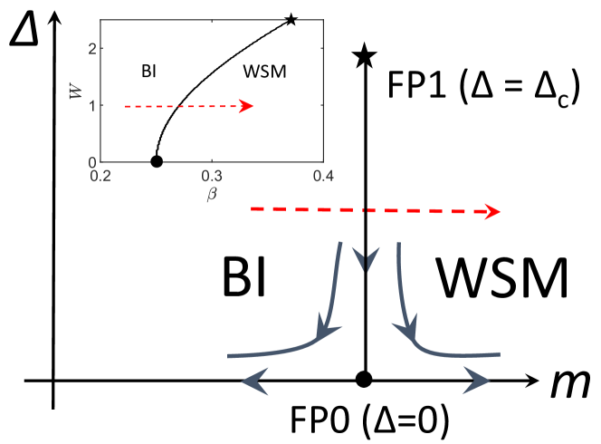
Figure 1: (color online) Schematic of the quantum phase transition between BI and WSM phases. The dark blue arrows denote renormalization group (RG) flows roy16arXiv ; luo18 . The criticality of the quantum phase transition at finite disorder strength is controlled by the critical point in the clean limit (‘FP0’ denoted by $\bullet$ mark). For the stronger disorder strength side, the quantum phase transition line is terminated by a quantum critical point (‘FP1’ denoted by $\star$ mark). Inset: a phase diagram of the tight-binding model for a three-dimensional layered Chern insulator with disorders cz-chen15 ; s-liu16 ; roy16arXiv ; luo18 . The disorder strength $W$ and interlayer coupling strength $\beta$ correspond to $\Delta$ and the effective mass $m$ respectively. The disorder strength $W$ as well as the interlayer coupling strength $\beta$ drives the quantum phase transition between BI (3D Chern insulator) and WSM phases. In Figs. 2 and 4, we change the effective mass $m$ (interlayer coupling strength $\beta$) with fixed $\Delta$ (disorder strength $W$); dashed red lines with arrow. In Fig. 3, the system is on the BI-WSM phase transition line. In the lower panel of Fig. 3, the system is on (or very close to) the FP1.

Eq. (4) generates all the scaling properties of the zero-energy conductances near the BI-WSM phase transition. We start with tiny $m$ and renormalize many times until the relevant scaling variable $m$ goes far away from the critical point, say $m^{\prime}=1$. Solving $b$ in favor for small $m$, we obtain a scaling function of the conductances as,

$$G_{\mu}(L_{z},L_{\perp},\Delta,m)=\Phi_{\mu}(m^{\frac{1}{2}}L_{z},mL_{\perp},m^{|y_{\Delta}|}\Delta).$$ (5)

For smaller $m$, we may replace the third argument by zero. The conductance scaling function depends on the linear dimension of system size along the dipole direction and that along the perpendicular directions with different exponents in $m$. This unconventional scaling form comes from the spatially anisotropic scale invariant property at the clean-limit fixed point.

To test this scaling function in numerical simulations, we take a tetragonal geometry, $L_{x}=L_{y}=L_{\perp}=\eta L^{2}_{z}$ with fixed geometric parameter $\eta$, to reduce Eq. (5) into a single parameter scaling form,

$$G_{\mu}(L_{z},L_{\perp}=\eta L^{2}_{z},\Delta,m)=\phi_{\mu}(m^{\frac{1}{2}}L_{z};\eta).$$ (6)

Using the same tetragonal geometry, we numerically calculate the conductances of a tight-binding model for a layered Chern insulator with disorders cz-chen15 ; s-liu16 ; roy16arXiv ; luo18 ; supplemental . In the tight-binding model, we fix a disorder strength $W$ and change an interlayer coupling strength $\beta$ (inset of Fig. 1). When the coupling strength exceeds a critical value $\beta_{c}$, the electronic system undergoes the quantum phase transition from BI phase ($\beta<\beta_{c}$) to WSM phase with a pair of Weyl nodes ($\beta>\beta_{c}$). The same quantum phase transition can be induced by a change of the disorder strength $W$ with constant $\beta$. Criticality of the quantum phase transition is controlled by the gapless theory in the clean limit, Eq. (2), where $\delta\beta=\beta-\beta_{c}$ is proportional to the effective mass $m$ in Eq. (2). In the WSM phase, the pair of the Weyl nodes appear at ${\bm{k}}_{\rm MM}=(0,0,\pm k_{z,c})$, where $k_{z,c}\propto\sqrt{\delta\beta}$. In the finite-size tight-binding model calculation, we choose $\eta=1/25$ and $(L_{z},L_{\perp})=(18,13)$, $(20,16)$, $(24,23)$, $(26,27)$, $(30,36)$, $(32,41)$, all of which satisfy $L_{z}=\eta L^{2}_{z}$ approximately. The conductance along the $\mu$ direction $G_{\mu}$ is calculated by the transfer matrix method with the periodic boundary conditions for the transverse directions. For $G_{x}(G_{z})$, we take 40 (5000) samples to obtain their distribution functions.

Fig. 2 shows $G_{x}$ and $G_{z}$ as a function of $\delta\beta\cdot\ L^{2}_{z}$ for the constant $W$. Almost all the numerical data fit in the proposed novel single parameter scaling form, Eq. (6). Especially, the data with larger system sizes near the critical point collapse into the form better, indicating the validity of the single parameter scaling form. The conductances in the WSM phase side show oscillatory behaviors as a function of $\delta\beta L^{2}_{z}$. In the WSM phase, the Weyl points appear at ${\bm{k}}_{\rm MM}=(0,0,\pm k_{z,c})$. The finite-size system with the periodic (fixed) boundary condition can feel these Weyl nodes only when $k_{z,c}$ becomes equal to $2\pi/L_{z}$ ($\pi/L_{z}$) times integer. Thus, the conductances show peaks when $L_{z}k_{z,c}$ matches integer times $2\pi$ ($\pi$) supplemental . Since $k_{z,c}$ scales $\sqrt{\delta\beta}$, the conductances show the oscillatory behaviors as a function of $\delta\beta L^{2}_{z}$. Notice also that $G_{z}$ at the critical point takes a vanishingly small value, while the critical conductance value of $G_{x}$ is much larger. The distinction can be attributed to the spatial anisotropy in the clean-limit fixed point supplemental .

Figure 2: (color online) $G_{x}$ (upper) and $G_{z}$ (lower) as a function of $\delta\beta\cdot L_{z}^{2}$ with the tetragonal geometry ($L_{\perp}=\eta L^{2}_{z}$ with $\eta=1/25$) and different $L_{z}$. We take a set of parameters in the tight-binding model in Refs. s-liu16 ; supplemental as $(W,\beta)=(1,\beta_{c}+\delta\beta)$ with $\beta_{c}=0.271$. The disorder strength $W$ corresponds to $\Delta$ in Fig. 1 and Eq. (6). $\delta\beta$ is proportional to the effective mass $m$ in Fig. 1 and Eqs. (2) and (6). Insets: $G_{x}$ (upper) and $G_{z}$ (lower) as a function of $\delta\beta$ with different $L_{z}$.

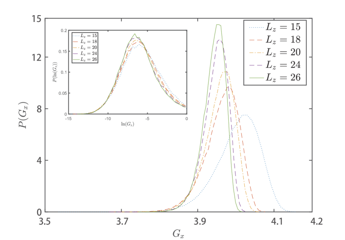
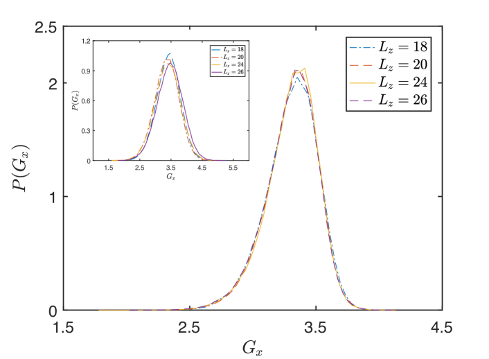
Figure 3: (color online) (upper) Critical conductance distribution of $G_{x}$ (inset: that of $G_{z}$) on the BI-WSM phase boundary. We take a set of parameters in the tight-binding model supplemental as $(W,\beta)=(1,0.271)$ (lower) Critical conductance distributions of $G_{x}$ on (or in proximity to) the critical point (‘FP1’ in Fig. 1) (main) $(W,\beta)=(2.1,0.338)$, (inset) $(W,\beta)=(2.45,0.366)$. We use the tetragonal geometry, $L_{\perp}=\eta L^{2}_{z}$ with $\eta=1/25$, $(L_{z},L_{\perp})=(15,9)$, $(18,13)$, $(20,16)$, $(24,23)$, $(26,27)$.

The critical conductance distribution (CCD) on the BI-WSM phase boundary also shows an unusual scaling behaviour, when compared to that of conventional disorder-driven quantum phase transitions slevin97 ; slevin00 ; slevin01prl ; slevin01prb ; kobayashi10 ; b-xu16 . To see this, let us begin with a general scaling relation between two distribution functions of critical conductance, before and after the renormalization;

$$P^{\prime}(G_{\mu},L^{\prime}_{\perp},L^{\prime}_{z},\Delta^{\prime},m^{\prime})=P(G_{\mu},L_{\perp},L_{z},\Delta,m).$$ (7)

Suppose that the criticality of a quantum phase transition is controlled by a fixed point with finite disorder strength ($\Delta=\Delta_{c}\neq 0$) and with the isotropic scaling ($L^{\prime}_{\perp}=bL_{\perp}$ and $L^{\prime}_{z}=bL_{z}$). CCD in such conventional quantum phase transition point depends only on a system geometry ($L_{\perp}/L_{z}$) and on universal properties encoded in the fixed point. Namely, after a certain times of the renormalization, $\Delta^{\prime}$ and others parameters already get (close) to a set of values at the fixed point, while $L^{\prime}_{\perp}$ and $L^{\prime}_{z}$ remain much larger than the lattice constant scale. Thereby, the right hand side of Eq. (7) is essentially equal to the left hand side with $\Delta^{\prime}=\Delta_{c}\neq 0$, where the ratio $L^{\prime}_{\perp}/L^{\prime}_{z}=L_{\perp}/L_{z}$ determines the CCD.

Our numerical simulation (upper panel of Fig. 3) indicates that CCD on the BI-WSM phase boundary essentially takes a form of the delta function, but the distribution becomes larger for smaller system. This is anticipated because the criticality of the phase transition is controlled by a fixed point (FP0) with zero disorder strength ($\Delta_{c}=0$). Besides, the renormalization needs to be truncated when either $L^{\prime}_{\perp}$ or $L^{\prime}_{z}$ reaches the lattice constant scale in the l.h.s. of Eq. (7). The truncation results in larger renormalized disorder $\Delta^{\prime}$ for smaller $L_{\perp}$ and $L_{z}$.

The BI-WSM phase transition line has an end point at a finite disorder strength $\Delta_{c}\neq 0$, which we dub ‘FP1’ as in Fig. 1. The critical end point is another scale-invariant fixed point and has two relevant scaling variables, $\delta\Delta\equiv\Delta-\Delta_{c}$ and $m$, and numerous irrelevant scaling variables. On such a fixed point, the disorder strength and the effective mass stay at $\Delta_{c}$ and $0$ respectively, while all the irrelevant scaling variables reduce to zero after the renormalization. Thus, the CCD calculated with the tetragonal geometry $L_{\perp}=\eta L^{2}_{z}$ is expected to be scale invariant for fixed geometric parameter $\eta$. To see the CCD scale invariance at the critical end point, we calculate the conductance distribution for a number of different disorder strength $W$ along the BI-WSM phase transition line. The BI-WSM phase transition line can be accurately determined by the self-consistent Born calculation. For a certain disorder strength along the BI-WSM boundary line, our numerical results indeed observe the CCD scale-invariant feature (lower panel of Fig. 3) as well as prominent kink-like features in the critical conductances $G_{x}$ and $G_{z}$ supplemental .

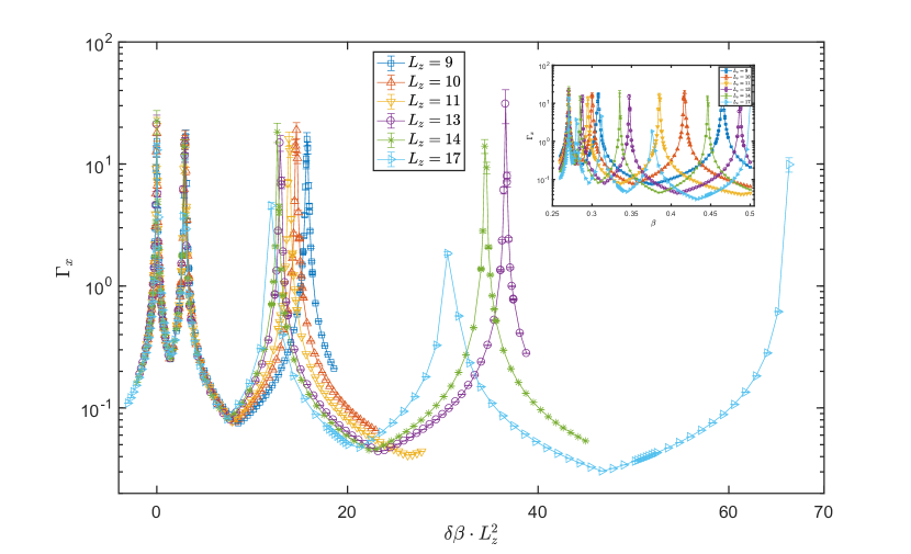
Figure 4: (color online) $\Gamma_{x}\equiv\xi_{x}/L_{z}^{2}$ as a function of $\delta\beta L_{z}^{2}$ near the BI-WSM phase transition point with $\Delta<\Delta_{c}$. We take a set of parameters in the tight-binding model supplemental as $(W,\beta)=(1,\beta_{c}+\delta\beta)$ with $\beta_{c}=0.2705$ and $\eta=1/10$. $\delta\beta$ is proportional to the effective mass $m$ defined in Eqs. (2) and (13). Inset: $\Gamma_{x}$ as a function of $\delta\beta$ with different $L_{z}$. An oscillatory behaviour of $\xi_{x}$ as a function of $\delta\beta$ is of the same origin as that of the conductance in Fig. 2 (see the text).

The zero-energy localization lengths at the BI-WSM phase transition also obey unconventional scaling function forms. From Eq. (3) at $E=0$, we obtain RG scaling relations of the localization length along the dipole ($z$) direction $\xi_{z}$ and that along the perpendicular ($xy$) direction $\xi_{x}$,

$$\xi^{\prime}_{x}(L^{\prime}_{x},L^{\prime}_{y},L^{\prime}_{z},\Delta^{\prime},m^{\prime})=b\xi_{x}(L_{x},L_{y},L_{z},\Delta,m),$$ (8)

$$\xi^{\prime}_{z}(L^{\prime}_{x},L^{\prime}_{y},L^{\prime}_{z},\Delta^{\prime},m^{\prime})=b^{\frac{1}{2}}\xi_{z}(L_{x},L_{y},L_{z},\Delta,m).$$ (9)

For $\Delta\leq\Delta_{c}$, $L^{\prime}_{x,y}=bL_{x,y}$, $L^{\prime}_{z}=b^{\frac{1}{2}}L_{z}$, $\Delta^{\prime}=b^{|y_{\Delta}|}\Delta$, $m^{\prime}=b^{-1}m$ with $b<1$. Henceforth, we omit dependences of the irrelevant parameter $\Delta$. The RG scaling relations lead to the following scaling forms of $\xi_{x}$ and $\xi_{z}$;

$$\xi_{x}(L_{x},L_{y},L_{z},m) =m^{-1}\Psi_{x}(mL_{x},mL_{y},m^{\frac{1}{2}}L_{z}),$$ (10)

$$\xi_{z}(L_{x},L_{y},L_{z},m) =m^{-\frac{1}{2}}\Psi_{z}(mL_{x},mL_{y},m^{\frac{1}{2}}L_{z}).$$ (11)

Eq. (11) gives a single-parameter scaling form for the quasi one-dimensional system ($L_{x,y}=L_{\perp}\ll L_{z}$) luo18 ;

$$\Gamma_{z}(L_{x}=L_{y}=L_{\perp},m)\equiv\xi_{z}/\sqrt{L_{\perp}}=\psi_{z}(mL_{\perp}).$$ (12)

To verify the scaling form of Eq. (10) in terms of the transfer matrix calculation mackinnon81 ; pichard81 , we set $L_{y}=\eta L^{2}_{z}$ and calculate $\xi_{x}$ for very large $L_{x}=10^{5}\sim 10^{7}$. For such a geometry, the localization length normalized by $L^{2}_{z}$ should show scaling invariance at the BI-WSM phase transition point ($m=0$);

$$\Gamma_{x}(L_{y}=\eta L^{2}_{z},L_{z},m)\equiv\xi_{x}/L^{2}_{z}=\psi_{x}(m^{\frac{1}{2}}L_{z};\eta).$$ (13)

To test this single parameter scaling form in the numerics, we take $\eta=1/10$, $(L_{z},L_{y})=(9,8)$, $(10,10)$, $(11,12)$, $(13,17)$, $(14,20)$, $(17,29)$, that approximately satisfy $L_{y}=\eta L^{2}_{z}$. Fig. 4 demonstrates that the $\Gamma_{x}$ with different $L_{z}$ near the phase transition point (small $\delta\beta L_{z}^{2}$ region) collapse into a single scaling function of $mL^{2}_{z}$.

In this paper, we clarified novel scaling theories of conductance, CCD and localization length in the quantum phase transition between three-dimensional BI and WSM phases. The idea in this paper can be also applied to a direct phase transition between ordinary band insulator (OI) and topological insulator (TI) phases shindou09prb ; kobayashi13 ; kobayashi14 , whose criticality is controlled by a clean-limit fixed point. The conductance scaling at the OI-TI phase transition is given by Eq. (1) with $\nu=1$, while the CCD on the boundary line takes a delta function form.

A recent transport experiment discovered a solid-state material that exhibits continuous BI-WSM phase transitions liang17 . Our paper reveals the universal critical properties of this continuous phase transition through the electric conductance. The results show that the conductance at the critical point is scaled by $L^{2}_{z}/L_{\perp}$: conventionally, the critical conductance is scaled by $L_{z}/L_{\perp}$. Such difference in the conductance scaling has significant impact on the transport experiment, compared to mere differences in the critical exponent.

Supplemental Material

I tight-binding model for a layered Chern insulator with disorder

In order to test the new scaling functions numerically, we use a two-orbital tight-binding model defined on a cubic lattice luo18 ; cz-chen15 ; s-liu16 . The model consists of an $s$ orbital and a $p=p_{x}+ip_{y}$ orbital on each cubic lattice site (${\bm{x}}$);

$${\cal H}= \sum_{{\bm{x}}}\Big{\{}\big{(}\epsilon_{s}+v_{s}({\bm{x}})\big{)}c^{\dagger}_{{\bm{x}},s}c_{{\bm{x}},s}+\big{(}\epsilon_{p}+v_{p}({\bm{x}})\big{)}c^{\dagger}_{{\bm{x}},p}c_{{\bm{x}},p}\Big{\}}+\sum_{{\bm{x}}}\Big{\{}-\sum_{\mu=x,y}\big{(}t_{s}c^{\dagger}_{{\bm{x}}+{\bm{e}}_{\mu},s}c_{{\bm{x}},s}-t_{p}c^{\dagger}_{{\bm{x}}+{\bm{e}}_{\mu},p}c_{{\bm{x}},p}\big{)}$$

$$+t_{sp}(c^{\dagger}_{{\bm{x}}+{\bm{e}}_{x},p}-c^{\dagger}_{{\bm{x}}-{\bm{e}}_{x},p}-ic^{\dagger}_{{\bm{x}}+{\bm{e}}_{y},p}+ic^{\dagger}_{{\bm{x}}-{\bm{e}}_{y},p})\!\ c_{{\bm{x}},s}-t^{\prime}_{s}c^{\dagger}_{{\bm{x}}+{\bm{e}}_{z},s}c_{{\bm{x}},s}-t^{\prime}_{p}c^{\dagger}_{{\bm{x}}+{\bm{e}}_{z},p}c_{{\bm{x}},p}+{\rm H.c.}\Big{\}}.$$ (14)

$\epsilon_{s}$, $\epsilon_{p}$ and $\upsilon_{s}(\bm{x})$, $\upsilon_{p}(\bm{x})$, are atomic energies for the $s$, $p$ orbital and on-site disorder potential of the $s$, $p$ orbital, respectively. The disorder potentials are uniformly distributed within $[-W/2,W/2]$ with identical probability distribution. $t_{s}$, $t_{p}$, and $t_{sp}$ are intralayer transfer integrals between $s$ orbitals of nearest neighboring two sites, that between $p$ orbitals, and that between $s$ and $p$ orbitals, respectively, while $t_{s}^{\prime}$ and $t_{p}^{\prime}$ are interlayer transfer integrals. ${\bm{e}}_{\mu}$ ($\mu=x,y$) are primitive translational vectors within a square-lattice plane. ${\bm{e}}_{z}$ is a primitive translational vector connecting neighboring square-lattice layers. In this paper, we take

$$t_{p} =t_{s},\ \ \epsilon_{s}=-\epsilon_{p}=2t_{s}+4t_{s}\beta,$$

$$t^{\prime}_{p} =-t^{\prime}_{s}=2t_{s}\beta,\ \ t_{sp}=\frac{4t_{s}}{3},$$

where we change an ‘interlayer coupling strength’ $\beta$. The tight-binding model without disorder ($W=0$) reduces to the following 2 by 2 Hamiltonian,

$$H({\bm{k}})={\bm{a}}({\bm{k}})\cdot{\bm{\sigma}}.$$

Here ${\bm{\sigma}}=(\sigma_{x},\sigma_{y},\sigma_{z})$ are Pauli matrices and

$$a_{z}({\bm{k}}) \equiv 2t_{s}(1+2\beta)-2t_{s}(\cos k_{x}a_{\perp}+\cos k_{y}a_{\perp})+4t_{s}\beta\cos k_{z}a_{z},$$ (15)

$$a_{x}({\bm{k}}) \equiv-\frac{8t_{s}}{3}\sin k_{y}a_{\perp},\ \ a_{y}({\bm{k}})\equiv-\frac{8t_{s}}{3}\sin k_{x}a_{\perp}.$$ (16)

For later clarity, we made explicit lattice constants of the cubic model along the $z$-direction $a_{z}$ and along the $xy$ directions $a_{\perp}$.

For $\beta<1/4$, the electronic system at the half filling ($E=0$) is in a 3-dimensional band insulator phase. For $\beta=1/4$, a pair of Weyl nodes is created at $E=0$ at the $\Gamma$ point. For $\beta>1/4$, the Weyl nodes appear at ${\bm{k}}=(0,0,\pm k_{z,c})$ with $\cos k_{z,c}=1/(2\beta)-1$. This gives out the clean-limit electronic phase diagram as in the inset of Fig. 1 in the main text. Throughout the paper, the unit of the disorder strength $W$ is taken to be $4t_{s}$.

II conductance oscillations in Weyl semimetal phases

The two-terminal conductances in the WSM phase side show oscillatory behaviors as a function of $\delta\beta L^{2}_{z}$ (Fig. 2 in the main text). For positive $\delta\beta$ (WSM phase side), the Weyl points appear at ${\bm{k}}_{\rm MM}=(0,0,\pm k_{z,c})$. In the following, we show that the oscillation behaviour of $G_{z}$ (lower panel of Fig. 2 in the main text) comes from a ‘commensurability effect’ between $\pi/L_{z}$ and the Weyl node position along the $k_{z}$-axis, $k_{z,c}$.

In the transfer-matrix calculation of the two-terminal conductance $G_{z}$, two lead Hamiltonians ($z<0$ and $z>L_{z}$) are attached to the bulk Hamiltonian ($0<z<L_{z}$). The lead Hamiltonian comprises of $L_{\perp}\times L_{\perp}$ number of decoupled one-dimensional chains,

$${\cal H}_{\rm lead}=-t_{0}\sum_{\bm{x}}\sum_{a=s,p}\Big{(}c^{\dagger}_{{\bm{x}}+{\bm{e}}_{z},a}c_{{\bm{x}},a}+{\rm H.c.}\Big{)}.$$ (17)

This has $2\times L^{2}_{\perp}$ number of the zero-energy eigenstates with positive velocity along the $z$ direction. The zero-energy conductance is calculated from transmission coefficient between the zero-energy eigenstates in the $z<0$ region and those in the $z>L_{z}$ region. Contrary to the large number of the zero-energy eigenstates in the two leads, the bulk has less than four zero-energy eigenstates. Thereby, most of the zero-energy states injected from the lead regions are reflected backward at the two contacts. For the bulk wavefunction’s point of view, this situation can be effectively described by the fixed boundary condition imposed at $z=0$ and $z=L_{z}$.

The finite-size system with the fixed boundary condition sees the two Weyl nodes only when $k_{z,c}$ becomes equal to $\pi/L_{z}$ times integer. Thus, the zero-energy conductance along the $z$ direction is expected to show a peak structure when $k_{z,c}\cdot L_{z}$ becomes integer times $\pi$. In Fig. 5, we replot the data points of $G_{z}$ in Fig. 2 in the main text as a function of $k_{z,c}\cdot L_{z}$. Here $k_{z,c}$ in the presence of finite disorder strength is accurately determined by the self-consistent Born calculation. In Fig. 5, one can see that peak structures appear when $k_{z,c}\cdot L_{z}=n\pi$ ($n=2,3,4,5,\cdots$).

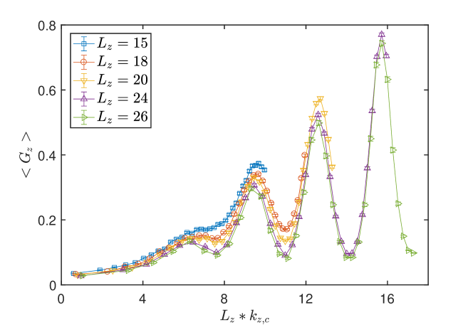
Figure 5: (color online) $G_{z}$ as a function of $k_{z,c}L_{z}$ reproduced from the same data stream as in Fig. 2 in the main text. $k_{z,c}$ in the presence of finite disorder strength is determined by the self-consistent Born calculation. The interval between neighboring peaks in the plot is around $\pi$.

III marginal scaling variables and critical conductance

$b_{2}$ and $v$ in the effective continuum model, Eq. (1) in the main text, do not change under the renormalization. In other words, ‘FP0’ with different $b_{2}$ and $v$ comprise a surface of fixed points (‘fixed surface’) in a higher-dimensional parameter space that includes these two marginal scaling variables (see Fig. 6). The scaling functions of the zero-energy conductance and localization length depend on these two scaling variables as;

$$G_{\mu}(L_{\perp},L_{z},m,b_{2},v,\Delta,\cdots) =\Phi_{\mu}(mL_{\perp},m^{\frac{1}{2}}L_{z},b_{2},v,m^{-y_{\Delta}}\Delta,\cdots),$$ (18)

$$\xi_{x}(L_{x},L_{y},L_{z},m,b_{2},v,\Delta,\cdots) =m^{-1}\Psi_{x}(mL_{x},mL_{y},m^{\frac{1}{2}}L_{z},b_{2},v,m^{-y_{\Delta}}\Delta,\cdots).$$ (19)

From Eq. (15), one can see that the interlayer coupling strength $\beta$ changes the effective mass $m$ as well as one of the two marginal parameters, $b_{2}=2t_{s}\beta a^{2}_{z}$ [$v$ does not depend on $\beta$; see Eq. (16)]. Thereby, the $b_{2}$-dependence in Eqs. (18,19) can result in larger deviations of the data points from the single parameter scaling forms in Figs 2, 4 in the main text.

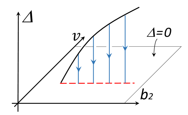
Figure 6: (color online) Schematic figure that explains how the BI-WSM phase boundary line in the inset of Fig. 1 in the main text is seen in the three-dimensional parameter space subtended by the disorder strength $\Delta$, and two marginal parameters $b_{2}$ and $v$. The $\Delta=0$ plane in the figure is a fixed surface, within which any points do not move under the renormalization. The blue arrows denote RG flows, connecting the BI-WSM phase boundary line with finite disorders (black solid line) with its projection onto the fixed surface (red dotted line).

The scale-invariant value of critical conductance $G_{x}$ varies with the disorder strength along the BI-WSM phase boundary line (see Fig. 7). This is apparently inconsistent with the $\Delta$-dependence proposed in Eqs. (5,6) in the main text. The discrepancy can be resolved, once we take into account $b_{2}$ and $v$-dependences as in Eqs. (18,19). Namely, under the renormalization, the critical conductance value on the BI-WSM boundary line with finite disorder $\Delta$ can be equated to that on its projection line at $\Delta=0$ (see Fig. 6);

$$\lim_{L_{z}\rightarrow+\infty}G_{\mu}(L_{\perp}=\eta L^{2}_{z},L_{z},m=0,b_{2},v,\Delta,\cdots)=\lim_{L^{\prime}_{z}\rightarrow+\infty}G_{\mu}(L^{\prime}_{\perp}=\eta{L^{\prime}_{z}}^{2},L^{\prime}_{z},m=0,b_{2},v,\Delta=0,\cdots).$$ (20)

Here $b_{2}$ in Eq. (20) is given by the critical interlayer coupling strength $\beta_{c}$; Eq. (15) gives $b_{2}=2t_{s}\!\ \beta_{c}\!\ a^{2}_{z}$. Meanwhile, the critical interlayer coupling strength changes with the disorder strength (see the inset of Fig. 1 in the main text). Thus, the left hand side of Eq. (20) can vary with the disorder strength $\Delta$ through the $b_{2}$-dependence of the right hand side with $b_{2}=2t_{s}\!\ \beta_{c}(\Delta)\!\ a^{2}_{z}$.

The critical conductance value of $G_{\mu}$ is given as a function of the two marginal scaling variables as well as the geometric parameter $\eta$ with $L_{\perp}=\eta L^{2}_{z}$. From the dimensional analysis, the scaling form is given by

$$\lim_{L_{z}\rightarrow+\infty}G_{\mu}(L_{\perp}=\eta L^{2}_{z},L_{z},m=0,b_{2},v,\Delta=0,\cdots)=\Theta_{\mu}\Big{(}\frac{b_{2}\eta a_{\perp}}{va^{2}_{z}}\Big{)},$$ (21)

where $a_{z}$ and $a_{\perp}$ are lattice constants of the tight-binding model along the dipole ($z$) direction and the perpendicular ($xy$) directions respectively. The scaling function $\Theta_{\mu}(x)$ can be evaluated explicitly. For the zero-energy conductance along the perpendicular directions ($\mu=x,y$), the function is given by

$$\Theta_{x}\Big{(}\frac{b_{2}\eta a_{\perp}}{va^{2}_{z}}\Big{)}=\lim_{L_{z}\rightarrow+\infty}\lim_{E\rightarrow+0}\frac{e^{2}}{\hbar}\sum_{j_{y}}\sum_{j_{z}}\int^{\infty}_{0}\frac{dk_{x}}{2\pi}\frac{\partial E_{\bm{k}}}{\partial k_{x}}\delta(E-E_{\bm{k}}),$$ (22)

where

$$E_{\bm{k}} \equiv\sqrt{b^{2}_{2}k^{4}_{z}+v^{2}(k^{2}_{x}+k^{2}_{y})},$$ (23)

$$k_{y} =\frac{2\pi}{L_{\perp}a_{\perp}}j_{y},\!\ k_{z}=\frac{2\pi}{L_{z}a_{z}}j_{z},\!\ L_{\perp}=\eta L^{2}_{z},$$ (24)

with two integers $j_{y},j_{z}=0,\pm 1,\pm 2,\cdots$. Note that there exists a subtlety in the order of the two limits in Eqs. (22), $\lim_{E\rightarrow+0}$ and $\lim_{L_{z}\rightarrow+\infty}$. When we take $E$ to be zero first and then take $L_{z}$ to be infinite, Eq. (22) reduces to $e^{2}/h$ times a number of those zero-energy eigenstates that carry positive velocities along the $x$ direction. The quantum critical point of the magnetic dipole model ($\Delta=m=0$) has only one such zero-energy eigenstate. The quantization in $e^{2}/h$ is obviously inconsistent with the numerical observations in Fig. 2 in the main text and Fig. 7. The discrepancy can be resolved, once we reconsider the order of the two limits.

In the transfer-matrix calculation of the two-terminal conductance, a whole system consists of the bulk Hamiltonian and two lead Hamiltonians that are attached to the bulk. For the lead Hamiltonian, we employ a ‘flux’ model as in Eq. (17). The zero-energy conductance is calculated from the transmission coefficient between the zero-energy eigenstates of the lead Hamiltonian in the $z<0$ region and those in the $z>L_{z}$ region. Such zero-energy eigenstates are not eigenstates of the bulk Hamiltonian. Instead, they are superpositions of those eigenstates of the bulk Hamiltonian that distribute around $E=0$. For such cases, it is more natural taking the two limits simultaneously rather than taking $E$ to be strictly zero from the outset. For a finite-size system with the tetragonal geometry, the eigen energy near $E=0$ is discretized by either $\frac{4\pi^{2}\!\ b_{2}}{(L_{z}a_{z})^{2}}$ or $\frac{2\pi\!\ v}{L_{\perp}a_{\perp}}$. We thus set the single particle energy $E$ in Eq. (22) to be $\frac{2\pi\!\ v\gamma}{L_{\perp}a_{\perp}}$. Here small $\gamma$ represents a dimensionless quantity that quantifies nature of the contact between lead and bulk. Generally, $\gamma$ is smaller for a better contact.

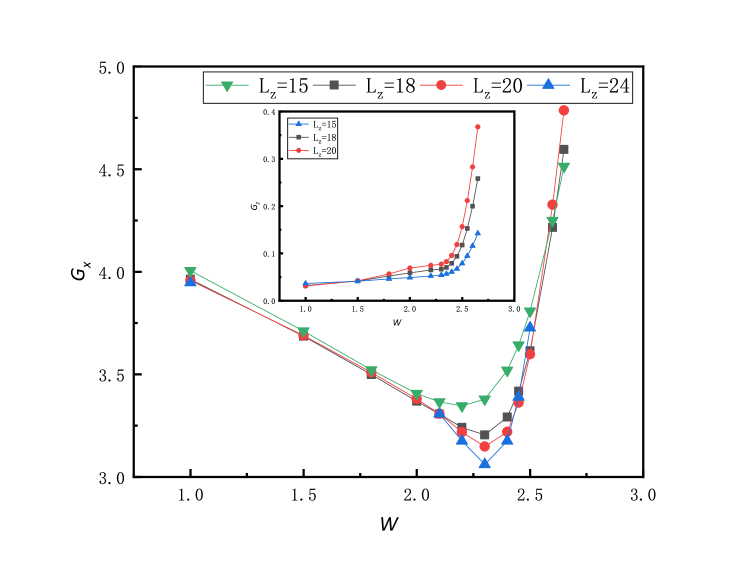
Figure 7: (color online) Critical conductance value of $G_{x}$ (inset: that of $G_{z}$) with $10^{5}$ samples as a function of the disorder strength $W$ along the BI-WSM phase transition line. The BI-WSM phase transition line is accurately determined by the self-consistent Born calculation.

The critical conductance along the $x$ direction is calculated in this intermediate limit as,

$$\Theta_{x}\Big{(}\frac{b_{2}\eta a_{\perp}}{va^{2}_{z}}\Big{)} =\lim_{L_{z}\rightarrow+\infty}\frac{e^{2}}{\hbar}\sum_{j_{y}}\sum_{j_{z}}\int^{\infty}_{0}\frac{dk_{x}}{2\pi}\frac{\partial E_{\bm{k}}}{\partial k_{x}}\delta(E-E_{\bm{k}})_{|E=\frac{2\pi v\gamma}{L_{\perp}a_{\perp}}}$$

$$=\frac{e^{2}}{h}\sqrt{\frac{v\gamma^{3}a^{2}_{z}}{2\pi b_{2}\eta a_{\perp}}}\frac{\sqrt{\pi}\!\ \Gamma\big{(}\frac{1}{4}\big{)}}{2\Gamma\big{(}\frac{7}{4}\big{)}}=\frac{e^{2}}{h}\sqrt{\frac{v\gamma^{3}a^{2}_{z}}{2\pi b_{2}\eta a_{\perp}}}\times 3.49\cdots,$$ (25)

where $\Gamma(x)$ is the Gamma function. The critical conductance along the dipole ($z$) direction is calculated in the same limit with $E=\frac{2\pi v\delta}{L_{\perp}a_{\perp}}$,

$$\Theta_{z}\Big{(}\frac{b_{2}\eta a_{\perp}}{va^{2}_{z}}\Big{)}=\lim_{L_{z}\rightarrow+\infty}\frac{e^{2}}{\hbar}\sum_{j_{x}}\sum_{j_{y}}\int^{\infty}_{0}\frac{dk_{z}}{2\pi}\frac{\partial E_{\bm{k}}}{\partial k_{z}}\delta(E-E_{\bm{k}})_{|E=\frac{2\pi v\delta}{L_{\perp}a_{\perp}}}=\frac{e^{2}}{h}\pi\delta^{2}.$$ (26)

Here $\gamma$ and $\delta$ are generally different from each other. Namely, $\gamma$ characterizes the contact between the lead and the $yz$ plane of the bulk Hamiltonian Eq. (14), while $\delta$ characterizes a contact between the lead with th $xy$ plane of Eq. (14). For the tight-binding model described above, $b_{2}=2t_{s}\beta a^{2}_{z}$, $v=\frac{8t_{s}}{3}a_{\perp}$, and $\eta=1/25$. This gives $(b_{2}\eta a_{\perp})/(va^{2}_{z})=0.81/100$ at $\beta=\beta_{c}=0.27\cdots$. For $\gamma=0.4$ and $\delta=0.1$, we have

$$G_{x}=\frac{e^{2}}{h}\times 3.91\cdots,\ \ \ G_{z}=\frac{e^{2}}{h}\times 0.0314\cdots.$$ (27)

These values are consistent with the order of the critical conductance values shown in Fig. 2 in the main text. Notice also that Eq. (26) has no explicit $b_{2}$ dependence. This is consistent with a weak $W$-dependence of the critical conductance value $G_{z}$ along the BI-WSM phase boundary line as in the inset of Fig. 7.

IV density of states

According to the preceding theories roy16arXiv ; luo18 , the density of states at a single-particle energy $E$ follows $\rho(E,\Delta,m)=m^{d-\frac{3}{2}}\Omega(m^{-1}E)$ around the BI-WSM phase transition line ($d=3$). A universal scaling function $\Omega(x)$ vanishes quadratically in small $x$ region (‘magnetic monopole regime’), while it diverges as $x^{\frac{3}{2}}$ in large $x$ region (‘magnetic dipole regime’). Fig. 8 demonstrates a crossover between these two different critical regions.

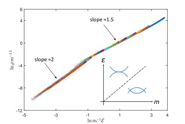
Figure 8: (color online) Log-Log plot of $m^{-d+\frac{3}{2}}\rho(E)$ as a function of $m^{-1}E$. We take a set of parameters in the tight-binding model Eq. (14) as $(W,\beta)=(1,0.271+\delta\beta)$ and $0<\delta\beta<0.25$. $\delta\beta$ is proportional to the effective mass $m$ in Eq. (1) in the main text. The density of states $\rho(E)$ is calculated in terms of the kernel polynomial expansion method. For data with $\beta$ larger/smaller than 0.29, we set the Chebyshev expansion order $N$ to be $N=2000/1500$.

References

(1) P. W. Anderson, Phys. Rev. 109, 1492 (1958).
(2) F. J. Wegner, Zeitschrift fur Physik B Condensed Matter 25, 327 (1976).
(3) E. Abrahams, P. W. Anderson, D. C. Licciardello, and T. V. Ramakrishnan,
Phys. Rev. Lett. 42, 673 (1979).
(4) A. MacKinnon and B. Kramer, Phys. Rev. Lett. 47, 1546 (1981).
(5) J. -L. Pichard, and G. Sarma, J. Phys. C14, L127 (1981).
(6) P. W. Anderson, D. J. Thouless, E. Abrahams, and D. S. Fisher, Phys. Rev. B
22, 3519 (1980).
(7) K. Slevin, P. Markos, and T. Ohtsuki, Phys. Rev. Lett. 86, 3594 (2001).
(8) E. P. Wigner, The Annals of Mathematics 53, 36 (1951).
(9) F. J. Dyson, Journal of Mathematical Physics 3, 140 (1962).
(10) F. J. Dyson, Journal of Mathematical Physics 3, 1199 (1962).
(11) M. R. Zirnbauer, Journal of Mathematical Physics 37, 4986 (1996).
(12) A. Altland and M. R. Zirnbauer, Phys. Rev. B 55, 1142 (1997).
(13) B. Shapiro, Phys. Rev. Lett. 65, 1510 (1990).
(14) A. Cohen and B. Shapiro, Int. J. Mod. Phys. B 06, 1243 (1992).
(15) K. Slevin and T. Ohtsuki, Phys. Rev. Lett. 78, 4083 (1997).
(16) K. Slevin, T. Ohtsuki, and T. Kawarabayashi, Phys. Rev. Lett. 84, 3915 (2000).
(17) J. Cardy, Scaling and Renormalization in Statistical Physics (Cambridge Lecture Notes in
Physics, Cambridge, 1996).
(18) B-J. Yang, M. S. Bahramy, R. Arita, H. Isobe, E-G. Moon, and N. Nagaosa,
Phys. Rev. Lett. 110, 086402 (2013).
(19) D. Carpentier, A. A. Fedorenko, and E. Orignac, Europhysics Letters, 102, 67010 (2013).
(20) B-J. Yang, E-G. Moon, H. Isobe, and N. Nagaosa, Nat. Phys. 10, 774 (2014).
(21) B. Roy, R. J. Slager, and V. Juricic, arXiv:1610.08973 (2016).
(22) X. Luo, B. Xu, T. Ohtsuki, and R. Shindou, Phys. Rev. B 97, 045129 (2018).
(23) J-R. Wang, W. Li, G. Wang, C.-J. Zhang, arXiv:1802.09050 (2018).
(24) S. Murakami, New Journal of Physics 9, 356 (2007).
(25) L. Balents, ‘Weyl electrons kiss’, Physics 4, 36 (2011).
(26) H. Weng, C. Fang, Z. Fang, B. A. Bernevig, and X. Dai, Phys. Rev. X 5, 011029 (2015).
(27) S. Y. Xu, I. Belopolski, N. Alidoust, M. Neupane, G. Bian, C. Zhang, R. Sankar, G. Chang,
Z. Yuan, C. C. Lee, S. M. Huang, H. Zheng, J. Ma, D. S. Sanchez, B. K. Wang, F. C. Bansil, A. Chou,
P. P. Shibayev, H. Lin, S. Jia, and M. Z. Hasan, Science, 349, 613 (2015).
(28) B. Q. Lv, H. M. Weng, B. B. Fu, X. P. Wang, J. Miao, Ma, P. Richard, X. C. Huang, L. X. Zhao,
G. F. Chen, Z. Fang, X. Dai, T. Qian, and H. Ding, Phys. Rev. X 5, 031013 (2015).
(29) E. Fradkin, Phys. Rev. B 33, 3263 (1986).
(30) P. Goswami, and S. Chakravarty, Phys. Rev. Lett. 107, 196803 (2011).
(31) S. V. Syzranov, V. Gurarie, and L. Radzihovsky, Phys. Rev. B 91, 035133 (2015).
(32) S. V. Syzranov, L. Radzihovsky and V. Gurarie, Phys. Rev. Lett. 114, 166601 (2015).
(33) C. Z. Chen, J. Song, H. Jiang, Q. F. Sun, Z. Wang, and X. C. Xie, Phys. Rev. Lett.
115, 246603 (2015).
(34) S. Liu, T. Ohtsuki, and R. Shindou, Phys. Rev. Lett. 116, 066401 (2016).
(35) See Supplemental Materials for detailed information of the tight-binding model,
oscillation behaviours of the conductances in the WSM phase, critical conductance values at the
BI-WSM phase boundary line, their kink-like feature at the quantum critical point (FP1), and density
of states scaling near the BI-WSM phase transition point.
(36) K. Slevin and T. Ohtsuki, Phys. Rev. B 63, 045108 (2001).
(37) K. Kobayashi, T. Ohtsuki, H. Obuse, and K. Slevin, Phys. Rev. B 83,
165301 (2010).
(38) B. Xu, T. Ohtsuki and R. Shindou, Phys. Rev. B 94, 220403 (2016).
(39) R. Shindou, and S. Murakami, Phys. Rev. B 79, 045321 (2009).
(40) K. Kobayashi, T. Ohtsuki, and K. I. Imura, Phys. Rev. Lett. 110, 236803 (2013).
(41) K. Kobayashi, T. Ohtsuki, and K. I. Imura, and I. F. Herbut, Phys. Rev. Lett.
112, 016402 (2014).
(42) Tian Liang, Satya Kushwaha, Jinwoong Kim,
Quinn Gibson, Jingjing Lin, Nicholas Kioussis,
Robert J. Cava, N. Phuan Ong, Science Advances, 3, e1602510 (2017).