Exact solution of Ginzburg’s $\Psi$-theory for the Casimir force in ⁴He superfluid film

Abstract

We present an analytical solution of the Ginzburg’s $\Psi$-theory for the behavior of the Casimir force in a film of ⁴He in equilibrium with its vapor near the superfluid transition point, and we revisit the corresponding experiments Garcia and Chan (1999) and Ganshin et al. (2006) in terms of our findings. We find reasonably good agreement between the $\Psi$-theory predictions and the experimental data. Our calculated force is attractive, and the largest absolute value of the scaling function is $1.848$, while experiment yields $1.30$. The position of the extremum is predicted to be at $x=(L/\xi_{0})(T/T_{\lambda}-1)^{1/\nu}=\pi$, while experiment is consistent with $x=3.8$. Here $L$ is the thickness of the film, $T_{\lambda}$ is the bulk critical temperature and $\xi_{0}$ is the correlation length amplitude of the system for $T>T_{\lambda}$.

I Introduction

I.1 Critical Casimir force near the $\lambda$ transition in ⁴He

It is now a well established experimental fact Garcia and Chan (1999); Ganshin et al. (2006) that the thickness of a helium film in equilibrium with its vapor decreases near and below the bulk transition into a superfluid state. The phenomenon has been discussed theoretically in a series of works; see, e.g., Refs. Krech and Dietrich (1992a, b); Zandi et al. (2004); Dantchev et al. (2005); Maciòłek et al. (2007); Zandi et al. (2007); Maciòłek et al. (2007); Hucht (2007); Dohm (2013); Vasilyev (2015). Among the methods used are renormalization group techniques Krech and Dietrich (1992a, b), mean-field type theories Zandi et al. (2007); Maciòłek et al. (2007) and Monte Carlo calculations Dantchev et al. (2005); Hucht (2007); Vasilyev (2015). It should be noted that in all of the above approaches it is assumed that the microscopic molecular interactions are not altered by the transition and that the observed change in the thickness thus results from the cooperative behavior of the constituents of the fluid system. Furthermore, the overall behavior of the force is in a relatively good agreement with finite-size critical point scaling theory Barber (1983); Cardy (1988); Privman (1990); Parry and Evans (1990); Brankov et al. (2000).

An inspection of the range of theoretical approaches used to study the Casimir force in helium films reveals that the problem has, so far, not been studied in the context of the so-called $\Psi$-theory of Ginzburg and co-authors Ginzburg and Sobaynin (1976); Ginzburg and Sobyanin (1982). This theory has been used by Ginzburg, et. al., to describe a variety of phenomena observed in Helium films and represents a portion of the research on Helium for which Ginzburg was recently awarded the Nobel prize in physics. In the current study we aim to fill that gap by applying $\Psi$ theory to calculate the critical Casimir force of a helium film that is subject only to short-ranged interactions, which is to say we neglect the van der Waals interaction between the film and its substrate.

We study the Casimir force in a horizontally positioned liquid ⁴He film supported on a substrate when that film is in equilibrium with its vapor. We will do this for temperatures at, and close to, the critical temperature, $T_{\lambda}$, of ⁴He at its bulk phase transition from a normal to a superfluid state.

I.2 Some data and facts from the experiment

The continuous phase transition in ⁴He from a normal to a superfluid state, referred to as the $\lambda$ transition because of the temperature dependence of the specific heat, occurs at a temperature Ginzburg and Sobaynin (1976) $T_{\lambda}=2.172$ ^∘K at a saturated-vapor pressure $p_{\lambda}=0.05$ atm and density Wilks (1967); Ginzburg and Sobyanin (1982) $\rho_{\lambda}=0.1459$ g/cm³. We note that while the density changes continuously through the transition its temperature gradient varies discontinuously Wilks (1967); Donelly and Barenghi (1998).

The critical exponents of systems, that belong to the $O(2)$ universality class of $O(n)$, $n\geq 2$ of systems with continuous symmetry of the order parameter, are Kleinert and Schulte-Frohlinde (2001); Zinn-Justin (2002)

$$\alpha = -0.011\pm 0.004,\nu=0.6703\pm 0.0013,$$

$$\eta = 0.0354\pm 0.0025.$$ (1)

Since hyperscaling holds, all critical exponents can be determined from, say, $\nu$ and $\eta$ using the appropriate scaling relations.

I.3 The Casimir force

Finite-size scaling theory Barber (1983); Cardy (1988); Privman (1990); Parry and Evans (1990); Brankov et al. (2000) for systems in which hyperscaling holds predicts a Casimir force of a system with a film geometry $\infty^{d-1}\times L$ of the form

$$F_{\rm Cas}(T,L)=L^{-d}X_{\rm Cas}(a_{t}\hat{t}L^{1/\nu}).$$ (2)

Here $X_{\rm Cas}$ is a universal scaling function that depends on the bulk and surface universality classes, $\hat{t}=(T-T_{\lambda})/T_{\lambda}$, and $a_{t}$ is a nonuniversal metric factor. Helium 4 belongs to the $O(2)$ bulk universality class and the boundary conditions on a helium film on a solid substrate that is in equilibrium with vapor are Dirichlet, in that the superfluid order parameter vanishes at the boundaries.

The Casimir force $F_{\rm Cas}(T,L)$ can be expressed in terms of an excess pressure $P_{L}(T)-P_{b}(T)$:

$$F_{\rm Cas}(T,L)=P_{L}(T)-P_{b}(T)$$ (3)

Here $P_{L}$ is the pressure on the finite system, while $P_{b}$ is the pressure in the infinite system. The Casimir force results from finite size effects, which are especially pronounced and of universal character near a critical point of the system. The above definition is equivalent to another, commonly used, relationship Evans (1990); Krech (1994); Brankov et al. (2000)

$$F_{\rm Cas}(T,L)\equiv-\frac{\partial\omega_{\rm ex}(T,L)}{\partial L}=-\frac{\partial\omega_{L}(T,L)}{\partial L}-P_{b},$$ (4)

where $\omega_{\rm ex}=\omega_{L}-L\,\omega_{b}$ is the excess grand potential per unit area, $\omega_{L}$ being the grand canonical potential of the finite system, again per unit area, and $\omega_{b}$ is the grand potential per unit volume of the infinite system. The equivalence between the definitions Eq. (3) and Eq. (4) arises from the observation that $\omega_{b}=-P_{b}$ while for the finite system with surface area $A$ and thickness $L$ one has $\omega_{L}=\lim_{A\to\infty}\Omega_{L}/A$, with $-\partial\omega_{L}(T,L)/\partial L=P_{L}$.

I.4 On the Casimir force in a class of systems

It is possible to derive a simple expression for the Casimir force in systems in which the order parameter is found by minimizing a potential that does not explicitly depend on the coordinate perpendicular to the film surface. For purposes of notation we denote the spatial coordinate perpendicular to the substrate by $z$. We consider systems in which the grand potential per unit area ${\cal\omega_{A}}$ is obtained by minimizing the functional

$${\cal\omega_{A}}=\int_{0}^{L}{\cal L}\left[\phi(z),\dot{\phi}(z)\right]dz,$$ (5)

where $\phi(z)$ is the local value of the order parameter at coordinate $z$, and $\dot{\phi}(z)\equiv d\phi(z)/dz$. We take $\cal L$ to be of the form

$$\mathcal{L}=\frac{1}{2}\dot{\phi}^{2}(z)-f[\phi(z)].$$ (6)

Following Gelfand and Fomin (Gelfand and Fomin, 1963, pp. 54-56) it is easy to show that the functional derivative of ${\cal\omega_{A}}$ with respect to the independent variable $z$ at $z=L$ is

$$-\left(\frac{\delta{\cal\omega_{A}}}{\delta z}\right)\Bigg{|}_{z=L}=-\left(\dot{\phi}\frac{\partial{\cal L}}{\partial\dot{\phi}}-{\cal L}\right)\Bigg{|}_{z=L}.$$ (7)

Taking into account the physical meaning of this functional derivative and performing the requisite calculations we obtain

$$P_{L}\equiv\left(\frac{\delta{\cal\omega_{A}}}{\delta z}\right)\Bigg{|}_{z=L}=\left(\dfrac{1}{2}\dot{\phi}^{2}+f(\phi)\right)\Bigg{|}_{z=L}.$$ (8)

The extrema of the functional ${\cal\omega_{A}}$ are determined by the solutions of the corresponding Euler-Lagrange equation

$$\dfrac{d}{dz}\frac{\partial{\cal\omega_{A}}}{\partial\dot{\phi}}-\frac{\partial{\cal\omega_{A}}}{\partial\phi}=0,$$ (9)

which leads to

$$\dfrac{d}{dz}\dot{\phi}+\frac{\partial f}{\partial\phi}=0.$$ (10)

Multiplying by $\dot{\phi}$ and integrating one obtains the corresponding first integral of the above second-order differential equation. The result is

$$\dfrac{1}{2}\dot{\phi}^{2}+f(\phi)={\rm const}=P_{L}.$$ (11)

Thus, the expression for $P_{L}$ has the same values at any point of the liquid film.

Let now assume that the boundary conditions are such that there is a point at which $\dot{\phi}=0$ and let $\phi_{0}$ be the value of $\phi$ at that point. Then we arrive at the very simple expression for the pressure on the boundaries of the finite system

$$P_{L}=f(\phi_{0}).$$ (12)

When the system is infinite the gradient term decreases with distance from a boundary, asymptoting to zero in the bulk within the type of theories we consider. It is easy to verify that the bulk pressure is

$$P_{b}=f(\phi_{b}),$$ (13)

where $\phi_{b}$ is the solution of the equation $\partial f/\partial\phi=0$, for which $\omega_{b}=-f(\phi)$ attains its minimum. The excess pressure, and hence the Casimir force, is

$$F_{\rm Cas}\equiv P_{L}-P_{b}=f(\phi_{0})-f(\phi_{b}).$$ (14)

The above expression, as we will see, is very convenient for the determination of the Casimir force in a system that can be described by a functional of the type given in Eq. (5). It has previously been used for systems described by the Ginzburg-Landau-Wilson functional Zandi et al. (2007); Dantchev et al. (2016); Note1 .

II The model

We now consider a film with thickness $L$ of liquid ⁴He that is in equilibrium with its vapor. We suppose the film to be parallel to the $(x,y)$ plane and its thickness to be along the $z$ axis. A constituent of the liquid film with total density $\rho$ is in the superfluid state with density $\rho_{s}(z)$ while the other one with density $\rho_{n}(z)$ is in the normal state. Obviously

$$\rho(z)=\rho_{n}(z)+\rho_{s}(z).$$ (15)

We consider two order parameters: a one-component order parameter $\rho_{n}$ to represent the normal fluid and two-component parameter $\Psi_{s}=\eta\exp(i\varphi)$ to stand for the superfluid portion of it. As usual, we take $\eta=\eta(z)$ and $\varphi=\varphi(z)$ to be real valued functions and, thus, $|\Psi_{s}|=\eta$ with the identification that

$$\rho_{s}=m|\Psi_{s}|^{2}=m\eta^{2},$$ (16)

where $m$ is the mass of the helium atom. A spatial gradient of the phase of the $\Psi_{s}$ function gives rise to the superfluid velocity via the relationship

$$\vec{v}_{s}=\frac{\hbar}{m}\nabla\varphi.$$ (17)

In the remainder of this article we consider only the case of a fluid at rest. Then one can take $\Psi_{s}$ to be a real function characterized solely by its amplitude $\eta$.

In terms of $\rho_{s}=m|\Psi_{s}|^{2}$ and $\rho_{n}$, the total amount of helium atoms in the fluid (normalized per unite area) is

$$\rho\equiv\frac{1}{L}\int_{0}^{L}\left[\rho_{s}(z)+\rho_{n}(z)\right]dz=\frac{1}{L}\int_{0}^{L}\rho(z)dz,$$ (18)

where the value of the overall average density $\rho$ is fixed by the chemical potential $\mu$. The above equation intertwines the profiles $\rho_{s}$ and $\rho_{n}$. For $\rho_{s}$ the natural boundary conditions at both the substrate-fluid interface and the fluid - vapor interfaces are

$$\rho_{s}(0)=\rho_{s}(L)=0\Leftrightarrow\Psi_{s}(0)=\Psi_{s}(L)=0.$$ (19)

The corresponding natural boundary conditions for $\rho_{n}$ depend on the interface. At the liquid-vapor interface one has

$$\rho_{n}(L)=\rho_{b}(T),$$ (20)

where $\rho_{b}(T)$ is the bulk density of the liquid helium at temperature $T$; at the substrate-liquid interface one has the so-called “dead” layers. In these layers ⁴He has solid-like properties, i.e., it does not possess a properties of a liquid, and it is immobilized at the boundary. This implies that there is some sort of close packing of the helium atoms. The number of layers is generally small—from two well below $T_{\lambda}$ to the order of 10 in the vicinity of that temperature. This can be thought of as a sort of adjusted thickness of the liquid films and will be ignored in our theory. Thus, we will assume that the boundary condition (20) is fulfilled at the both boundaries of the system, i.e., that

$$\rho_{n}(0)=\rho_{n}(L)=\rho_{b}(T).$$ (21)

Since we are addressing a spatially inhomogeneous problem, its proper treatment requires the minimization of the total thermodynamic potential ${\cal\omega_{A}}(\mu,T)$ Ginzburg and Sobyanin (1982); Sobyanin (1973), which is normalized per unit area, simultaneously with respect to $\Psi(z)$ and $\rho(z)$. Hereafter the dot will mean a differentiation with respect to the coordinate $z$.

A realization of the model within the so-called $\Psi$ theory

We take as our basic variables $\rho_{s}$ and $\rho$. We assume that they both vary within the film, so our system will depend on $\rho_{s}$ and $\rho$ and their gradients $\dot{\rho_{s}}$ and $\dot{\rho}$. If however, the gradient of $\rho$ is small, spatial derivatives of $\rho$ can be neglected. For temperatures well below the liquid-vapor critical point we will take $\rho$ to be a constant within the film, i.e., $\rho$ is $z$-independent. This implies near the $\lambda$ point one can treat helium as an incompressible liquid. This is what is done in Ginzburg and Sobaynin (1976) and Sobyanin (1973).

For the total thermodynamic potential ${\cal\omega_{A}}(\mu,T)$ per unit area one has

$${\cal\omega_{A}}(\mu,T)=\int_{-L/2}^{L/2}\left[\omega(\mu,T,\rho,\Psi_{s},\dot{\Psi_{s}})-\mu\rho\right]dz,$$ (22)

where $\omega(z)$ is the local density of this potential per unit area. Here $\omega=\omega_{I}(\mu,T,\rho)+\omega_{II}(\mu,T,\Psi_{s},\dot{\Psi_{s}})$, where $\omega_{I}$ is the local potential density of the normal fluid and $\omega_{II}$ is that of the superfluid. Since $\mu,T$ and $\rho$ are constants through the thickness of the film, one concludes that the terms $\omega_{I}$ and $\mu\rho$ will generate only bulk-like contributions, after the integration. For this reason we will not be interested in the specifics of these terms. Following Ginzburg and Sobyanin (1982), one can write

$$\omega_{II}=\omega_{II,0}+\frac{1}{2m}|-i\hbar\dot{\Psi}_{s}|^{2},$$ (23)

where $\omega_{II,0}=\omega_{II,0}(\mu,T,|\Psi_{s}|^{2})$ captures the corresponding bulk potential density of the infinite system. The gradient term can easily be rewritten in the equivalent forms

$$|-i\hbar\dot{\Psi}_{s}|^{2} = \frac{\hbar^{2}}{2m}\dot{\eta}^{2}+\frac{\hbar^{2}}{2m}\eta^{2}\dot{\varphi}^{2}$$ (24)

$$= \frac{\hbar^{2}}{8m^{2}}\frac{\dot{\rho}_{s}^{2}}{\rho_{s}}+\frac{1}{2}\rho_{s}v_{s}^{2}.$$

For a fluid at rest $v_{s}=0$.

In accord with Ginzburg and Sobyanin (1982); Ginzburg and Sobaynin (1976), we take $\omega_{II,0}$ to be of the form

$$\omega_{II,0}(\mu,T,|\Psi_{s}|^{2})=\dfrac{3T_{\lambda}\Delta C_{\mu}}{3+M}\left[-\tau|\tau|^{1/3}\left|\frac{\Psi_{s}}{\Psi_{s,e0}}\right|^{2}\right.$$ (25)

$$\left.+\frac{1-M}{2}|\tau|^{2/3}\left|\frac{\Psi_{s}}{\Psi_{s,e0}}\right|^{4}+\frac{M}{3}\left|\frac{\Psi_{s}}{\Psi_{s,e0}}\right|^{6}\right],$$

where $T_{\lambda}(\mu)$ is the $\lambda$-transition temperature in equilibrium with saturated vapor, $T_{\lambda}(\rho_{\lambda})=2.172$ K, $\rho_{\lambda}=0.146$ g cm^-3. Here

$$\tau=(T_{\lambda}(\mu)-T)/T_{\lambda}(\mu),$$ (26)

$\Delta C_{\mu}$ is the specific heat jump at the $\lambda$ point $\Delta C_{\mu}=\Delta C_{p}=0.76\times 10^{7}$ erg cm^-3 K^-1, $M$ is a parameter of the theory, and $\Psi_{s,e0}$ is the amplitude of the temperature dependence of the equilibrium value of $\Psi_{s}$ in bulk helium,

$$\Psi_{s,e}(\tau)=\Psi_{s,e0}\,\tau^{\beta}=0.23\times 10^{12}\,\tau^{1/3}\,{\rm cm}^{-3/2}.$$ (27)

The value of $\Psi_{s,e0}$ is, as usual Ginzburg and Sobyanin (1982), determined by the equation

$$\left(\frac{\partial\omega_{II,0}}{\partial|\Psi|^{2}}\right)_{\mu,T}=0$$ (28)

so as to be in accord with the experimental data

$$\rho_{se} = m|\Psi|^{2}=1.43\,\rho_{\lambda}T_{\lambda}^{2/3}\tau^{2/3}$$ (29)

$$= 0.35\,\tau^{2/3}\;{\rm g}\,{\rm cm}^{-3}=\rho_{s0}\,\tau^{\zeta}$$

with $\zeta\simeq 2\beta\simeq 2/3$. As is clear from Eq. (25), it is convenient to introduce the reduced variable

$$\psi=\frac{\Psi_{s}}{\Psi_{s,e0}}.$$ (30)

Then, Eq. (25) becomes

$$\omega_{II,0} = \dfrac{3T_{\lambda}\Delta C_{\mu}}{3+M}\left[-\tau|\tau|^{1/3}\left|\psi\right|^{2}\right.$$

$$\left.+\frac{1-M}{2}|\tau|^{2/3}\left|\psi\right|^{4}+\frac{M}{3}\left|\psi\right|^{6}\right].$$

The above expressions for $\omega$ and $\omega_{II}$ are consistent with a close approximation to the critical exponents in which $\alpha=0$, $\nu=2/3$ and the anomalous dimension exponent $\eta$ is zero. They define an effective $3$-dimensional theory for the behavior of the helium films. The best known values of the critical exponents $\alpha$ and $\nu$ for helium are given above, in Eq. (I.2).

The conditions for the minimum of ${\cal\omega_{A}}(\mu,T)$ are given by the corresponding Euler-Lagrange equations (see also Eqs. (1.3) and (1.4) in Sobyanin (1973), or Eq. (3.41) in Ginzburg and Sobaynin (1976)), which read

$$-\frac{\partial\omega_{I}}{\partial\rho}+\mu=0,$$ (32)

and

$$\frac{d}{dz}\frac{\partial\omega_{II}}{\partial\dot{\rho}_{s}}-\frac{\partial\omega_{II}}{\partial\rho_{s}}=0.$$ (33)

Note that the condition of $\rho$ being $z$-independent requires that the profiles $\rho_{n}(z)$ and $\rho_{s}(z)$ are connected; a change in one of them leads to a change in the other. We stress that the above arguments are not dependent on the actual functional form of $\omega$; they rely simply on the assumption that the overall density of the fluid inside the film does not change.

Within the $\Psi$ theory the type of phase transition in helium films from helium I to helium II depends crucially on the value of the parameter $M$ Ginzburg and Sobaynin (1976); Ginzburg and Sobyanin (1982). For $M<1$ this transition, as in bulk helium, is continuous, while for $M>1$ the transition in a film is first order. The value $M=1$ corresponds to a tricritical point. Thus, we use $M<1$ in our calculations. Obviously, the simplest case has $M=0$.

Keeping in mind Eq. (23) and Eq. (33) for the function $\Psi$, one obtains the equation

$$\frac{\hbar^{2}}{2m}\ddot{\Psi}=\Psi\frac{\partial\omega_{II}}{\partial|\Psi|^{2}},$$ (34)

or, in terms of the reduced variable $\psi$

$$\Psi_{s,e0}^{2}\,\frac{\hbar^{2}}{2m}\ddot{\psi}=\psi\frac{\partial\omega_{II}}{\partial|\psi|^{2}},$$ (35)

Introducing, as in Ginzburg and Sobaynin (1976); Ginzburg and Sobyanin (1982), the scaled spatial variable

$$\zeta_{0}=z/\xi_{0},$$ (36)

where, see Eq. (23) in Ginzburg and Sobyanin (1982), for $\xi_{0}$ one has

$$\xi_{0}=\frac{\hbar\Psi_{s,e0}}{\sqrt{2mT_{\lambda}\Delta C_{\mu}}}=\frac{\hbar}{m}\sqrt{\frac{\rho_{s,0}}{2T_{\lambda}\Delta C_{\mu}}}\simeq 1.63\times 10^{-8}{\rm cm}$$ (37)

with $\xi_{0}$ being the amplitude of the correlation function above the $\lambda$ point for the version of the theory with $M=0$, one can write the equation for the dimensionless function $\psi$ in the form

$$\ddot{\psi}=\dfrac{3}{3+M}\psi\left[-\tau|\tau|^{1/3}+(1-M)|\tau|^{2/3}\left|\psi\right|^{2}+M\left|\psi\right|^{4}\right].$$ (38)

Here the differentiation is to be understood with respect to the scaled variable $\zeta_{0}$. Eq. (38) is the main equation within the $\Psi$ theory one deals with.

The proper boundary conditions are

$$\psi(0)=0,\psi(L)=0,$$ (39)

but so that $\lim_{L\to\infty}\psi(L/2)=\psi(\infty)=\psi_{e}=\tau^{1/3}$.

III The behavior of the Casimir force

It is convenient to introduce the variables

$$\xi_{\tau}=\sqrt{\dfrac{3+M}{3}}\,\xi_{0}\,|\tau|^{-2/3},\quad\mbox{and}\quad\phi=\psi|\tau|^{-1/3},$$ (40)

where $\xi_{0}$ is given by Eq. (37). Then Eq. (38) becomes

$$\ddot{\phi}=\phi\left[-\textup{sign}(\tau)+(1-M)\left|\phi\right|^{2}+M\left|\phi\right|^{4}\right],$$ (41)

where the derivative is taken with respect to $\zeta_{\tau}$,

$$\zeta_{\tau}\equiv\frac{z}{\xi_{\tau}}=\frac{z}{L}\frac{L}{\xi_{\tau}}=\zeta_{L}x_{\tau},$$ (42)

with

$$\zeta_{L}=\frac{z}{L}\quad\mbox{and}\quad x_{\tau}=\frac{L}{\xi_{\tau}}.$$ (43)

Note that since $\xi_{\tau}$ depends on $M$, see Eq. (40), the scaling variable $x_{\tau}$, see Eq. (43), is also $M$-dependent. Note also that, in contrast to commonly utilized notations, $\tau>0$ corresponds to $T<T_{\lambda}$. Obviously, in equilibrium bulk helium, when $\ddot{\phi}=0$, one has $\phi\equiv\phi_{b}$ with $\phi_{b}=1$ for $T\leq T_{\lambda}$, and $\phi_{b}=0$ for $T>T_{\lambda}$.

Now we turn to the solution of this equation in a system with a film geometry.

Multiplying (41) by $\dot{\phi}$ and integrating, we obtain

$$\dot{\phi}^{2}+\textup{sign}(\tau)\phi^{2}-\dfrac{1}{2}(1-M)\phi^{4}-\dfrac{1}{3}M\phi^{6}=p,$$ (44)

where $p$ is a quantity that is $z$-independent. One should also note that $\dot{\phi}=0$ at $z=L/2$. Let us denote $\phi(z=L/2)=\phi_{0}$. Then one has

$$p=\textup{sign}(\tau)\phi_{0}^{2}-\dfrac{1}{2}(1-M)\phi_{0}^{4}-\dfrac{1}{3}M\phi_{0}^{6}.$$ (45)

Thus, for $\dot{\phi}^{2}$ one has

$$\dot{\phi}^{2}=\textup{sign}(\tau)(\phi_{0}^{2}-\phi^{2})-\dfrac{1}{2}(1-M)(\phi_{0}^{4}-\phi^{4})-\dfrac{1}{3}M(\phi_{0}^{6}-\phi^{6}).$$ (46)

At the boundary we have $\phi(0)=0$. This is the minimum value of $\phi$. For $T<T_{\lambda}$, i.e. $\tau>0$ the derivative is greater than zero for $\zeta_{\tau}$ in the interval from $\zeta_{\tau}=0$ to the middle of the system, where it vanishes when the profile levels off close to its bulk value of $\phi_{b}=1$. For $T>T_{\lambda}$, i.e. $\tau<0$, one finds that $\dot{\phi}^{2}\leq 0$ if $\phi(\zeta_{\tau})<\phi_{0}$ for any value of $\zeta_{\tau}$. Keeping in mind the fact that $\phi(0)=0$, we conclude that $\phi(\zeta_{\tau})=0$ is the only possible solution in this case.

Before proceeding to the technical details of the calculations let us note that, according to Eq. (11), one has

$$p=\dfrac{1}{2}P_{L},$$ (47)

where $P_{L}$ is the pressure on the boundaries of a system with size $L$, the behavior of which is mathematically described by the corresponding functional written in terms of the variable $\phi$. In terms of $\phi$ and $x_{\tau}$, Eq. (25) for $\omega_{\text{II},0}$ becomes

$$\beta\omega_{\text{II},0} = L^{-3}\sqrt{\frac{3+M}{3}}\beta T_{\lambda}\text{$\Delta$C}_{\mu}\xi_{0}^{3}$$

$$\times\;x_{\tau}^{3}\left(-\textup{sign}(x_{\tau})\phi^{2}+\frac{1}{2}(1-M)\phi^{4}+\frac{1}{3}M\phi^{6}\right).$$

The equation for the profile $\phi(\zeta_{\tau})$, $\tau>0$, reads

$$\zeta_{\tau}=\int_{0}^{\phi(\zeta_{\tau})}\frac{d\phi}{\sqrt{(\phi_{0}^{2}-\phi^{2})-\dfrac{1}{2}(1-M)(\phi_{0}^{4}-\phi^{4})-\dfrac{1}{3}M(\phi_{0}^{6}-\phi^{6})}},$$ (49)

complemented by the equation that determines $\phi_{0}$

$$\frac{1}{2}\dfrac{L}{\xi_{\tau}}=\int_{0}^{\phi_{0}}\frac{d\phi}{\sqrt{(\phi_{0}^{2}-\phi^{2})-\dfrac{1}{2}(1-M)(\phi_{0}^{4}-\phi^{4})-\dfrac{1}{3}M(\phi_{0}^{6}-\phi^{6})}}.$$ (50)

Introducing the variable $\phi=y\phi_{0}$, and after that performing the change of variables from $y^{2}\to y$ the above equation becomes

$$x_{\tau}\equiv\dfrac{L}{\xi_{\tau}}=\int_{0}^{1}\frac{dy}{\sqrt{y\left(1-y\right)\left[1-\dfrac{1}{2}(1-M)\phi_{0}^{2}\left(1+y\right)-\dfrac{1}{3}M\phi_{0}^{4}\left(1+y^{2}+y\right)\right]}}.$$ (51)

The integral on the right-hand side of Eq. (51) leads naturally to expressions in involving elliptic functions.

III.1 The case $M=0$

In this case the expression for $p$ becomes

$$p=\textup{sign}(\tau)\phi_{0}^{2}-\dfrac{1}{2}\phi_{0}^{4},$$ (52)

while for $x_{\tau}$, from Eq. (51), one has

$$x_{\tau}=\int_{0}^{1}\frac{1}{\sqrt{y(1-y)\left(\text{sgn}(\tau)-\frac{1}{2}\phi_{0}^{2}(1+y)\right)}}\,dy.$$ (53)

From Eq. (53) it is clear that $x_{\tau}$ is a well defined quantity only for $0\leq\phi_{0}<1$. It is also easy to check that $x_{\tau}$ is a monotonically increasing function of $\phi_{0}$, with $x_{\tau}(\phi_{0}=0)=\pi$. The last implies that one will have a non-zero solution for $\phi_{0}$ and, therefore, for $\phi(\zeta_{\tau})$ for $x_{\tau}>\pi$. Let us also note that from Eq. (52) one concludes $0\leq p<1/2$.

Taking the integral in Eq. (53), when $0\leq\phi_{0}<1$ one derives

$$x_{\tau}=\frac{2\sqrt{2}}{\sqrt{2-\phi_{0}^{2}}}K\left(\sqrt{\frac{\phi_{0}^{2}}{2-\phi_{0}^{2}}}\right).$$ (54)

It is easy to check that the right-hand side of Eq. (54) is a monotonically increasing function of $\phi_{0}$. Thus, one can uniquely invert this equation, thereby determining $\phi_{0}(x_{\tau})$.

As noted previously, when $\phi_{0}\geq\phi(\zeta_{\tau})$, one is directly led to the conclusion that $\phi(\zeta_{\tau})=0$ is the only allowed solution of Eq. (46).

Summarizing the information from the two above sub-cases $\tau>0$ and $\tau<0$, and performing the corresponding numerical evaluations for the behavior of the Casimir force in the case $M=0$ one obtains the result shown in Fig. 1.

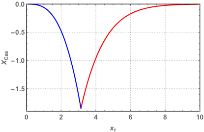
Figure 1: The behavior of the Casimir force within the $\Psi$ theory when $M=0$.

In order to obtain this curve we make use of the first integral Eq. (52), its relation to the pressure in the finite system Eq. (47), the corresponding easily obtainable expression for the bulk pressure, as well as the relation Eq. (53) between $\phi_{0}$ and $x_{t}$, and, finally Eq. (III), which becomes

$$\beta F_{\rm Cas}(T,L) = \dfrac{1}{2}\beta T_{\lambda}\Delta C_{\mu}\xi_{0}^{3}\;x_{\tau}^{3}\left[p(\phi_{0}(x_{t}))-1/2\right]L^{-3}$$ (55)

$$\simeq 0.119\;x_{\tau}^{3}\left[p(\phi_{0}(x_{t}))-1/2\right]L^{-3}.$$

The evaluation of the above expression leads us to the curve displayed in Fig. 1 with

$$X_{\rm Cas}(x_{\tau})=0.119\;x_{\tau}^{3}\left[p(\phi_{0}(x_{t}))-1/2\right].$$ (56)

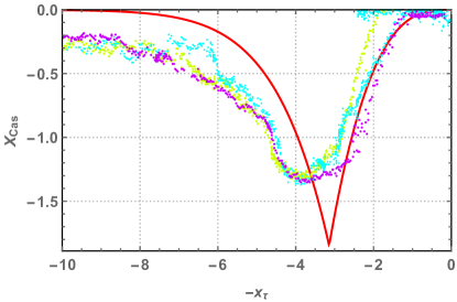
Figure 2: A comparison of the experimental data of the Casimir force, the scattered curves, reported in Ganshin et al. (2006) with the prediction of the $\psi$ theory when $M=0$, the solid curve. The position of the minimum within the $\Psi$-theory is at $x_{\tau}=\pi$, while the experiment delivers $x_{\tau}=3.8$. The minimal value of the force is $-1.848$ within the theory, while within the experiment it is $-1.30$.

Solving Eq. (49), for the order parameter profile $\phi(\zeta_{\tau})$ in the case $M=0$ one has

$$\phi(\zeta_{\tau})=\phi_{0}\;\text{sn}\left(\zeta_{\tau}\sqrt{1-\frac{\phi_{0}^{2}}{2}}\Bigg{|}\sqrt{\frac{\phi_{0}^{2}}{2-\phi_{0}^{2}}}\right),$$ (57)

where $\phi_{0}$, as a function of $x_{\tau}$, is to be determined from Eq. (54). Here ${\rm sn}$ is the Jacobi elliptic function ${\rm sn}(u|m)$ Abramowitz and Stegun (1970).

Fig. 2 presents a comparison of the experimental determination Ganshin et al. (2006) of the Casimir force with the prediction of the $\psi$ theory with $M=0$. When transferring the experimental data of Ganshin et al. (2006), given in terms of $(T/T_{\lambda}-1)L^{1/\nu}$ to the variable $L/(\xi_{0}|t|^{1/\nu})$ we have used the value of $\nu$ given in Eq. (I.2), and the data of $\xi_{0}=1.2$ $\AA$ reported in Ihas and Pobell (1974). We observe that while the position of the minimum within the $\Psi$-theory is at $x_{\tau}=\pi$, the experiment yields $x_{\tau}=3.8$. The minimal value of the scaling function of the force is $-1.848$ within the theory, and $-1.30$ in the experiment.

III.2 The case $0<M<1$

From Eq. (51) it is easy to check that $x_{\tau}$ is a monotonically increasing function of $\phi_{0}$, with $x_{\tau}(\phi_{0}=0,M)=\pi$. The last implies that one will have a non-zero unique solution for $\phi_{0}$ and, therefore, for $\phi(\zeta_{\tau})$ only when $x_{\tau}>\pi$. The above statements are valid for any value of $0\leq M<1$.

The Casimir force is now given by the expression

$$\beta F_{\rm Cas}(T,L;M) = \dfrac{1}{2}\beta T_{\lambda}\Delta C_{\mu}\xi_{0}^{3}\;\sqrt{\dfrac{3+M}{3}}\;x_{\tau}^{3}(M)$$

$$\times\left[p(\phi_{0}(x_{t},M),M)-\dfrac{3+M}{6}\right]L^{-3}$$

$$\simeq 0.119\sqrt{\dfrac{3+M}{3}}\;x_{\tau}^{3}\left[p-\dfrac{3+M}{6}\right]L^{-3}.$$

Evaluating the integral in Eq. (51), for $\phi_{0}$ one obtains the equation

$$x_{\tau}\equiv\dfrac{L}{\xi_{\tau}}=\frac{4\sqrt{3}}{b}K(k)$$ (59)

where $K(k)$ is the complete elliptic integral of elliptic modulus

$$k=\sqrt{2\sqrt{3}a}\;\frac{\phi_{0}}{b}$$ (60)

with

$$a = \sqrt{(3+M+2M\phi_{0}^{2})(1+M(3-2\phi_{0}^{2}))},$$

$$b = \sqrt{12-6M\phi_{0}^{4}+\phi_{0}^{2}(\sqrt{3}a-9(1-M))}.$$

Solving this equation for $\phi_{0}$, one finds $\phi_{0}=\phi_{0}(x_{\tau},M)$, where $x_{\tau}$ also depends on $M$ via Eq. (40) and Eq. (43).

A comparison of the Casimir force calculated in the case $M=0$, $M=0.5$ and $M=0.8$ is shown in Fig. 3. The position of the minimum stays unchanged but its absolute value increases with increasing $M$. Thus, the $M=0$ theory coincides most closely with the experimentally reported data.

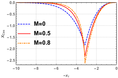
Figure 3: The behavior of the Casimir force within the $\psi$ theory when $M=0$, $M=0.5$ and $M=0.8$. The minimal value of the force gets deeper with increase of M.

The order parameter profile can be also obtained in an explicit form for the case $0\leq M<1$. Solving Eq. (49), for the order parameter profile $\phi(\zeta_{\tau}|M)$ one has

$$\phi(\zeta_{\tau}|M)=\frac{\sqrt{c}\,\phi_{0}\,\mathrm{sn}\left(\frac{b}{2\sqrt{3}}\zeta_{\tau}|k\right)}{\sqrt{1+c-\mathrm{sn}\left(\frac{b}{2\sqrt{3}}\,\zeta_{\tau}|k\right)^{2}}},$$ (61)

where

$$c=\frac{\sqrt{3}a+M\left(2\phi_{0}^{2}-3\right)+3}{4M\phi_{0}^{2}}.$$ (62)

Here $\phi_{0}$, as a function of $x_{\tau}$, is to be determined from Eq. (59). Here ${\rm sn}$ again symbolizes the Jacobi elliptic function ${\rm sn}(u|m)$.

IV Discussion and concluding remarks

In the current study we have applied the $\Psi$-theory of Ginzburg and co-authors Ginzburg and Sobaynin (1976); Ginzburg and Sobyanin (1982) to evaluate the Casimir force in ⁴He film in equilibrium with its vapor. We have obtained an exact closed form expression for the force within this theory—see Eq. (55)—when the parameter of the theory $M=0$, and Eq. (III.2) for $0\leq M<1$. We have found the best agreement between the theory and experiment for $M=0$. The corresponding result for the scaling function of the Casimir force is shown in Fig. 1 and the comparison with the experiment is shown in Fig. 2. We conclude that there is reasonably good agreement between this model theory and experiment. One should note, however, some important differences. In the $\Psi$ theory there is a sharp two-dimensional phase transition with long-ranged order below the critical temperature of the finite system, while in the helium system one expects a Kosterlitz-Thouless type transition. This feature is not captured by the $\Psi$-theory. Also missing are the Goldstone modes and surface wave contributions that appear at low temperatures Zandi et al. (2004). The overall agreement between the result of the $\Psi$-theory and the experiment, shown in Fig. 2 is, however, much better than is provided by mean-field theory Zandi et al. (2007); there is no need to fit any parameter in $\Psi$ theory in order to achieve this agreement.