State measurement error-to-state stability results
based on approximate discrete-time models

Abstract

Digital controller design for nonlinear systems may be complicated by the fact that an exact discrete-time plant model is not known. One existing approach employs approximate discrete-time models for stability analysis and control design, and ensures different types of closed-loop stability properties based on the approximate model and on specific bounds on the mismatch between the exact and approximate models. Although existing conditions for practical stability exist, some of which consider the presence of process disturbances, input-to-state stability with respect to state-measurement errors and based on approximate discrete-time models has not been addressed. In this paper, we thus extend existing results in two main directions: (a) we provide input-to-state stability (ISS)-related results where the input is the state measurement error and (b) our results allow for some specific varying-sampling-rate scenarios. We provide conditions to ensure semiglobal practical ISS, even under some specific forms of varying sampling rate. These conditions employ Lyapunov-like functions. We illustrate the application of our results on numerical examples, where we show that a bounded state-measurement error can cause a semiglobal practically stable system to diverge.

I Introduction

Digital controller design for nonlinear systems can be substantially more complicated than for linear systems. One of the main obstacles to the design of adequate digital controllers for nonlinear (continuous-time) plants is that even if a continuous-time plant model is known, the corresponding exact discrete-time model, i.e. the model that describes the state evolution at the sampling instants, can be difficult or even impossible to obtain. This happens because the computation of the exact discrete-time model requires knowledge of the solution to a nonlinear differential equation.

Interesting existing results address controller design based on an approximate discrete-time model of the plant and ensure the stabilization of the original continuous-time plant in a practical sense [1, 2, 3, 4]. A general framework for stabilization of disturbance-free sampled-data nonlinear systems via approximate discrete-time models was developed in [1, 2] with further generalization for continuous-time plants with disturbances in [5, 3, 4] and for observer design in [6]. All of these approches are specifically suited to uniform-sampling, i.e. the sampling rate is constant during operation.

In many sampled-data control systems, the use of a non-uniform sampling period is necessary, usually imposed by performance requirements of the plant, hardware limitations or network communication constraints. The occurrence of non-uniform sampling is typical of Networked Control Systems (NCSs). The main feature of NCSs is that the different system components exchange data over a communication network. Results for control design based on approximate discrete-time models also exist for different NCS scenarios. In [7], controller design for nonlinear NCSs with time-varying sampling periods, time-varying delays and packet dropouts is considered, based on approximate discrete-time models constructed for nominal sampling period and delays. All of the results mentioned so far ensure practical stability properties for sufficiently small sampling periods, with ultimate bounds of decreasing size in correspondence with decreasing maximum sampling periods.

Related but conceptually different results exist for dual- or multi-rate sampling, where some constraint exists on how fast measurements can be taken [8, 9, 10]. These results give closed-loop practical stability warranties and employ approximate discrete-time models in order to predict the state evolution at the control update instants, since new measurements may not be available at each of these instants. Specifically, [10] proposes a multi-rate sampled-data scheme to stabilize a NCS via output feedback using discrete-time approximations. The results of [10] as well as those of [7] give practical stability and robustness warranties for deviations about a nominal situation.

Non-uniform sampling is also a feature of event-triggered control, where a triggering condition based on a continuous measurement of system variables (e.g. the system state) determines when the control action has to be updated [11, 12]. Strategies that also involve non-uniform sampling but require only sampled measurements are those of self-triggered control [13, 14, 12]. Self-triggered control computes both the control action and the next sampling instant at which the control action should be recomputed. In both event-triggered and self-triggered control, we may thus say that sampling is controller-driven, since the controller itself is in charge of computing the next sampling instant.

The objective of this paper is to provide practical stability results based on approximate discrete-time models, and allowing some specific non-uniform sampling scenarios. Our results are, however, independent of the mechanism employed to vary the sampling rate. In this context, the main contribution of the current paper is to provide conditions on the approximate discrete-time plant model and the control law in order to ensure closed-loop semiglobal-practical input-to-state stability (see Section II-B for the precise definition), where the ‘input’ is the state measurement error.

Our results are novel even for the uniform sampling case. The fact that state measurement errors be considered causes the analysis to become substantially different from that of disturbances affecting the plant dynamics (as in [3]). This is because if based on a perturbed state measurement, the control action will itself have some error, and this in turn will cause some intersample error additional to that introduced by the approximation in the discrete-time model. More specific differences between the given and existing results will be explained along the paper. The fact that some specific varying-sampling-rate scenarios be covered increases the applicability of our results. Related preliminary results dealing with closed-loop stability possibly under controller-driven sampling (without measurement errors) have been given in [15, 16].

The organization of this paper is as follows. This section ends with a brief summary of the notation employed throughout the paper. In Section II we state the problem and the required definitions and properties. Our main results are given in Section III. An illustrative example is provided in Section IV and concluding remarks are presented in Section V. The appendix contains the proofs of some intermediate technical points.

Notation: $\mathbb{R}$, $\mathbb{R}_{\geq 0}$, $\mathbb{N}$ and $\mathbb{N}_{0}$ denote the sets of real, nonnegative real, natural and nonnegative integer numbers, respectively. A function $\alpha:\mathbb{R}_{\geq 0}\to\mathbb{R}_{\geq 0}$ is of class-$\mathcal{K}$ (we write $\alpha\in\mathcal{K}$) if it is strictly increasing, continuous and $\alpha(0)=0$. It is class-$\mathcal{K}_{\infty}$ ($\alpha\in\mathcal{K}_{\infty}$) if in addition $\alpha(s)\rightarrow\infty$ as $s\rightarrow\infty$. A function $\beta:\mathbb{R}_{\geq 0}\times\mathbb{R}_{\geq 0}\to\mathbb{R}_{\geq 0}$ is of class-$\mathcal{KL}$ ($\beta\in\mathcal{KL}$) if $\beta(\cdot,t)\in\mathcal{K}$ for all $t\geq 0$, and $\beta(s,\cdot)$ is strictly decreasing asymptotically to $0$ for every $s$. We denote the identity function by id. We denote the Euclidean norm of a vector $x\in\mathbb{R}^{n}$ by $|x|$. Given a set $\mathcal{X}\subset\mathbb{R}^{n}$ we denote its $\epsilon$ neighborhood as $N(\mathcal{X},\epsilon):=\{x:\inf_{y\in\mathcal{X}}|x-y|\leq\epsilon\}$. We denote an infinite sequence as $\{T_{i}\}:=\{T_{i}\}_{i=0}^{\infty}$. For any sequences $\{T_{i}\}\subset\mathbb{R}_{\geq 0}$ and $\{e_{i}\}\subset\mathbb{R}^{m}$, and any $\gamma\in\mathcal{K}$, we take the following conventions: $\sum_{i=0}^{-1}T_{i}=0$ and $\gamma(\sup_{0\leq i\leq-1}|e_{i}|)=0$. Given a real number $T>0$ we denote by $\Phi(T):=\{\{T_{i}\}:\{T_{i}\}\subset(0,T)\}$ the set of all sequences of real numbers in the open interval $(0,T)$. For a given sequence we denote the norm $\|\{x_{i}\}\|:=\sup_{i\geq 0}|x_{i}|$.

II Preliminaries

II-A Problem statement

We consider the nonlinear continuous-time plant

$$\begin{split}\dot{x}&=f(x,u),\quad x(0)=x_{0},\\ \end{split}$$ (1)

where $x(t)\in\mathbb{R}^{n}$, $u(t)\in\mathbb{R}^{m}$ are the state and control vectors respectively and $f(0,0)=0$. As in [1], the function $f:\mathbb{R}^{n}\times\mathbb{R}^{m}\to\mathbb{R}^{n}$ is assumed to be such that for each initial condition and constant control, there exists a unique solution on some interval $[0,\tau)$ with $0<\tau\leq\infty$.

We consider that state measurements become available at time instants $t_{k}$, $k\in\mathbb{N}_{0}$, that satisfy $t_{0}=0$ and $t_{k+1}=t_{k}+T_{k}$, where $\{T_{k}\}_{k=0}^{\infty}$ is the sequence of corresponding sampling periods. As opposed to the uniform sampling case where $T_{k}=T$ for all $k\in\mathbb{N}_{0}$, the sampling periods $T_{k}$ may vary. We refer to this situation as Varying Sampling Rate (VSR). The control signal is assumed to be piecewise constant (i.e. zero-order hold is present) such that $u(t)=u(t_{k})=:u_{k}$ for all $t\in[t_{k},t_{k+1})$. We denote the state at the sampling instants by $x_{k}:=x(t_{k})$. The control action $u_{k}$ may depend on the state measurement $\hat{x}_{k}=x_{k}+e_{k}$, with $e_{k}$ the state measurement error, and also on the sampling period $T_{k}$, i.e. we have $u_{k}=U(\hat{x}_{k},T_{k})$. The dependence of the control action at time $t_{k}$, on the sampling period $T_{k}=t_{k+1}-t_{k}$ is possible in the following situations: (a) uniform sampling; (b) controller-driven sampling (such as self-triggered control [13], or others [17]). In the situation (a), the constant sampling period employed can be known before the controller is implemented. This is the setting in [2, 4, 3]. In (b), at each sampling instant $t_{k}$, the controller may select the next sampling instant $t_{k+1}$ and, thus, the current sampling period $T_{k}$. As a consequence, knowledge of $T_{k}$ can be employed in order to compute the current control action $u_{k}$. However, our results will be still valid in the particular case $u_{k}=\bar{U}(\hat{x}_{k})$, where the control law does not explicitly depend on the sampling period. In addition, our results are independent of the way in which the sampling periods $T_{k}$ may vary over time. Fig. 1 depicts the complete closed-loop system.

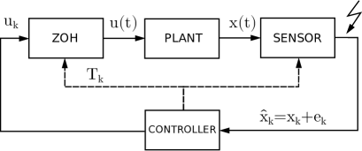
Figure 1: Schematic diagram of the controlled plant

The exact discrete-time model for a given nonlinear system is the discrete-time system whose state matches the state of the continuous-time system at every sampling instant. From (1), and given that the plant input $u$ is held constant over each sampling interval, it is clear that the state value at the next sampling instant, namely $x_{k+1}$, will depend on the current state value $x_{k}$, the current input value $u_{k}$, and the sampling period $T_{k}$. Hence, a discrete-time model for the case of zero-order hold and VSR can be written as

$$x_{k+1} =F^{e}(x_{k},u_{k},T_{k}),$$ (2)

where the superscript ^e stands for “exact”. Due to the fact that the solution to (1) does not necessarily exist for all future times, then the exact discrete-time model $F^{e}(\cdot,\cdot,\cdot)$ may be not defined for every $(x,u,T)\in\mathbb{R}^{n}\times\mathbb{R}^{m}\times\mathbb{R}_{\geq 0}$. However, we assume that $f$ in (1) has sufficient regularity so that for every pair of compact sets $\mathcal{X}\subset\mathbb{R}^{n}$ and $\mathcal{U}\subset\mathbb{R}^{m}$, there exists some $T^{*}>0$ so that $F^{e}(x,u,T)$ is defined for every $(x,u,T)\in\mathcal{X}\times\mathcal{U}\times[0,T^{*})$. The exact model $F^{e}$ is in general very hard or even impossible to obtain and thus some type of approximation may be necessary for the design of a stabilizing controller. A superscript ^a will be used to denote an approximate model:

$$x_{k+1} =F^{a}(x_{k},u_{k},T_{k}).$$ (3)

We will use ‘$F$’ with no superscript to denote any discrete-time model (either exact or approximate). Under the feedback law $u_{k}=U(\hat{x}_{k},T_{k})=U(x_{k}+e_{k},T_{k})$, the closed-loop discrete-time model becomes

$$x_{k+1} =F(x_{k},U(x_{k}+e_{k},T_{k}),T_{k})=:\bar{F}(x_{k},e_{k},T_{k}),$$ (4)

where the measurement error $e_{k}$ (disturbance) is regarded as an input. Hence, given a control law/discrete-time model pair $(U,F)$, the quantity $\bar{F}$ will denote the composition of $F$ and $U$ as shown in (4). Whenever required, we will write $x(k,\xi,\{e_{i}\},\{T_{i}\})$ to denote the solution of (4) at time $k$ with initial condition $\xi$ at $k=0$, and corresponding to the measurement error and sampling period sequences $\{e_{i}\}$ and $\{T_{i}\}$.

II-B Stability properties for varying sampling rate

Our objective is to provide conditions that ensure stability properties of the exact discrete-time closed-loop system under the varying-sampling-rate case. The following definition constitute a natural extension of the semiglobal practical ISS [18, 19, 3] property.

Definition II.1

The system (4) is said to be Semiglobal Practical ISS-VSR (SP-ISS-VSR) if there exist functions $\beta\in\mathcal{KL}$ and $\gamma\in\mathcal{K}_{\infty}$ such that for every $M>0$, $E>0$ and $R>0$ there exists $T^{\star}>0$ such that the solutions of (4) satisfy

$$|x_{k}|\leq\beta\left(|x_{0}|,\sum_{i=0}^{k-1}T_{i}\right)+\gamma\left(\sup_{0\leq i\leq k-1}|e_{i}|\right)+R,$$ (5)

for all $k\in\mathbb{N}_{0}$, all $\{T_{i}\}\in\Phi(T^{\star})$, all $|x_{0}|\leq M$ and all $\|\{e_{i}\}\|\leq E$. The function $\bar{F}$ is said to be SP-ISS-VSR if the system (4) defined by $\bar{F}$ is SP-ISS-VSR.

Remark II.2

Note that the sequences of constant sampling periods $\{T_{i}\}$ such that $T_{i}=T>0$ for all $i\in\mathbb{N}_{0}$ are included in the set $\Phi(T^{\star})$ whenever $T^{\star}>T$. This implies that if any of the above properties holds for a certain system then the respective properties for the uniform sampling case also hold.

Remark II.3

Setting $k=0$ in (5), it follows that $|x_{0}|\leq\beta(|x_{0}|,0)+R$ holds for every $x_{0}\in\mathbb{R}^{n}$ and every $R>0$. As a consequence, any function $\beta\in\mathcal{KL}$ characterizing SP-ISS-VSR has the additional property that $r\leq\beta(r,0)$ for all $r\geq 0$. This property will be repeatedly employed for the proof of our results.

II-C Model consistency with non-ideal state measurements

The next definition, as appears in [6, Definition 1], ensures that the mismatch between the solutions of the exact and approximate systems over one sampling period is bounded by a value that depends on the sampling period, uniformly over states and inputs in compact sets. This bound tends to zero in a specific way as the sampling period becomes smaller.

Definition II.4

The function $F^{a}$ is said to be consistent with $F^{e}$ if for each compact set $\Omega\subset\mathbb{R}^{n}\times\mathbb{R}^{m}$, there exist $\rho\in\mathcal{K}$ and $T_{0}>0$ such that, for all $(x,u)\in\Omega$ and all $T\in[0,T_{0}]$,

$$|F^{e}(x,u,T)-F^{a}(x,u,T)|\leq T\rho(T).$$ (6)

Definition II.4 is similar to the definition of one-step consistency in [1, Defintion 1]. However, the main difference lies in the fact that Definition II.4 is “open-loop” whereas Definition 1 of [1] involves the feedback law. In the current setting of imperfect state knowledge, consideration of the feedback law would be meaningless unless the state measurement error be also considered (cf. Defintion II.6 below).

The following lemma is a minor modification of Lemma 1 of [1] that gives sufficient conditions for the consistency of $F^{a}$ with $F^{e}$, based on $f$ and $F^{a}$, and hence without requiring knowledge of $F^{e}$. The required modification is due to the fact that in the current setting the feedback law cannot assume perfect knowledge of the state. The proof closely follows the proof of Lemma 1 of [1] but is given in the Appendix for completeness.

Lemma II.5

Suppose that

1. $F^{a}$ is consistent with $F^{\text{Euler}}$, where $F^{\text{Euler}}(x,u,T):=x+Tf(x,u)$, and

2. for every pair of compact sets $\mathcal{X}\subset\mathbb{R}^{n}$ and $\mathcal{U}\subset\mathbb{R}^{m}$, there exist $\rho\in\mathcal{K}$ and $M>0$ such that for all $(x,u),(y,u)\in\mathcal{X}\times\mathcal{U}$,

   1. $|f(y,u)|\leq M$,

   2. $|f(y,u)-f(x,u)|\leq\rho(|y-x|)$.

Then, $F^{a}$ is consistent with $F^{e}$.

The following definition extends the definition of multi-step consistency in [1] to the varying-sampling-rate scenario considered and to the case of state measurement errors.

Definition II.6

The pair $(U,F^{a})$ is said to be Multi-Step Error Consistent (MSEC) with $(U,F^{e})$ if, for each $L>0$, $\eta>0$ and compact sets $\mathcal{X}\subset\mathbb{R}^{n}$ and $\mathcal{E}\subset\mathbb{R}^{n}$, there exist a function $\alpha:\mathbb{R}_{\geq 0}\times\mathbb{R}_{\geq 0}\rightarrow\mathbb{R}_{\geq 0}$ and $T^{*}>0$ such that

$$|\bar{F}^{e}(x^{e},e,T)-\bar{F}^{a}(x^{a},e,T)| \leq\alpha(\delta,T)$$ (7)

for all $x^{e},x^{a}\in\mathcal{X}$ satisfying $|x^{e}-x^{a}|\leq\delta$, all $e\in\mathcal{E}$, and all $T\in(0,T^{*})$, and for all $\{T_{i}\}\in\Phi(T^{*})$ and $k\in\mathbb{N}$ such that $\sum_{i=0}^{k-1}T_{i}\leq L$ we have

$$\alpha^{k}(0,\{T_{i}\}) :=\overbrace{\alpha(\ldots\alpha(\alpha(}^{k}0,T_{0}),T_{1}),\ldots,T_{k-1})\leq\eta.$$ (8)

The next lemma constitutes the corresponding extension of [1, Lemma 2] and shows that under MSEC, the error between the approximate and exact solutions over a fixed time period is reduced by making the maximum sampling period smaller. The proof is given in the Appendix for the sake of completeness.

Lemma II.7

If $(U,F^{a})$ is MSEC with $(U,F^{e})$ then for each compact sets $\mathcal{X}\subset\mathbb{R}^{n}$ and $\mathcal{E}\subset\mathbb{R}^{n}$, and constants $L>0$ and $\eta>0$, there exists $\tilde{T}>0$ such that, if $\{T_{i}\}$, $\{e_{i}\}$ and $\xi$ satisfy

$$\{T_{i}\} \in\Phi(\tilde{T}), x^{a}(k,\xi,\{e_{i}\},\{T_{i}\}) \in\mathcal{X}, e_{k} \in\mathcal{E},$$ (9)

for all $k$ for which $\sum_{i=0}^{k-1}T_{i}\in[0,L]$, then, for these values of $k$

$$|\Delta x_{k}| :=|x^{e}(k,\xi,\{e_{i}\},\{T_{i}\})-x^{a}(k,\xi,\{e_{i}\},\{T_{i}\})|\leq\eta.$$ (10)

The next lemma gives a sufficient condition for MSEC. This lemma can be regarded as the corresponding extension of [1, Lemma 3].

Lemma II.8

If, for each compact sets $\mathcal{X}\subset\mathbb{R}^{n}$ and $\mathcal{E}\subset\mathbb{R}^{n}$ there exist $\rho_{0}\in\mathcal{K}$, a nondecreasing function $\sigma:\mathbb{R}_{\geq 0}\rightarrow\mathbb{R}_{\geq 0}$ and $T^{*}>0$ such that for all $T\in(0,T^{*})$ and all $x,y\in\mathcal{X}$, $e\in\mathcal{E}$ we have

$$|\bar{F}^{e}(x,e,T)-\bar{F}^{a}(y,e,T)| \leq T\rho_{0}(T)+(1+T\sigma(T))|x-y|$$ (11)

then, $(U,F^{a})$ is MSEC with $(U,F^{e})$.

Proof:

Let $L>0$ and $\eta>0$, and let $\mathcal{X}\subset\mathbb{R}^{n}$ and $\mathcal{E}\subset\mathbb{R}^{n}$ be compact sets. Define the compact set $\tilde{\mathcal{X}}:=N(\mathcal{X},\eta)$ and let $\tilde{\mathcal{X}}$ and $\mathcal{E}$ generate $\rho_{0}\in\mathcal{K}$, $\sigma$ and $T^{*}>0$. Select $\hat{T}>0$ sufficiently small so that $\hat{T}\leq T^{*}$ and $e^{\sigma(\hat{T})L}\rho_{0}(\hat{T})L\leq\eta$. Define

$$\alpha(\delta,T):=T\rho_{0}(T)+(1+T\sigma(T))\delta.$$ (12)

Let $x,y\in\mathcal{X}$ be such that $|x-y|\leq\delta$, let $e\in\mathcal{E}$, and $T\in(0,\hat{T})$. From (11) and (12), then (7) is satisfied. Consider $\{T_{i}\}\in\Phi(\hat{T})$. Using (12), we may recursively define $\eta_{0}:=0$ and, for $k\geq 1$,

$$\eta_{k} :=\alpha^{k}(0,\{T_{i}\})=T_{k-1}\rho_{0}(T_{k-1})+(1+T_{k-1}\sigma(T_{k-1}))\eta_{k-1}$$

Recursively employing the latter formula, we may write, for $k\geq 1$ and such that $\sum_{i=0}^{k-1}T_{i}\leq L$,

$$\eta_{k} =T_{k-1}\rho_{0}(T_{k-1})+\sum_{j=0}^{k-2}T_{j}\rho_{0}(T_{j})\prod_{i=j+1}^{k-1}(1+T_{i}\sigma(T_{i}))$$

$$\leq T_{k-1}\rho_{0}(T_{k-1})+\sum_{j=0}^{k-2}T_{j}\rho_{0}(T_{j})e^{\sigma(\hat{T})\sum_{j+1}^{k-1}T_{i}}$$

$$\leq T_{k-1}\rho_{0}(T_{k-1})+e^{\sigma(\hat{T})L}\sum_{j=0}^{k-2}T_{j}\rho_{0}(T_{j})$$

$$\leq e^{\sigma(\hat{T})L}\sum_{j=0}^{k-1}T_{j}\rho_{0}(T_{j})\leq e^{\sigma(\hat{T})L}\rho_{0}(\hat{T})\sum_{j=0}^{k-1}T_{j}$$

$$\leq e^{\sigma(\hat{T})L}\rho_{0}(\hat{T})L\leq\eta,$$

where we have used the facts that for every $a>0$, $1+a\leq e^{a}$, and $T_{i}<\hat{T}$ for every $i\in\mathbb{N}_{0}$. This shows that $(U,F^{a})$ is MSEC with $(U,F^{e})$. ∎

For the sake of completeness, we next state the definition of locally uniformly bounded control law as in [3, Defintion II.4].

Definition II.9

$U(x,T)$ is said to be locally uniformly bounded if for every $M>0$ there exist $T^{*}=T^{*}(M)>0$ and $C=C(M)>0$ such that $|U(x,T)|\leq C$ for all $|x|\leq M$ and $T\in(0,T^{*})$.

Lemma II.10 gives sufficient conditions for MSEC based on consistency (as per Definition II.4) and properties of the control law and approximate model.

Lemma II.10

Suppose that

1. $F^{a}$ is consistent with $F^{e}$ as per Definition II.4.

2. $U(x,T)$ is locally uniformly bounded as per Definition II.9.

3. For each compact sets $\mathcal{X},\mathcal{E}\subset\mathbb{R}^{n}$ there exist a nondecreasing function $\sigma:\mathbb{R}_{\geq 0}\rightarrow\mathbb{R}_{\geq 0}$ and $T_{1}>0$ such that for all $x,z\in\mathcal{X}$, $e\in\mathcal{E}$ and $T\in(0,T_{1})$ we have

   $$|\bar{F}^{a}(x,e,T)-\bar{F}^{a}(z,e,T)| \leq(1+T\sigma(T))|x-z|.$$ (13)

Then, $(U,F^{a})$ is MSEC with $(U,F^{e})$.

Proof:

Let $\mathcal{X}\subset\mathbb{R}^{n}$ and $\mathcal{E}\subset\mathbb{R}^{n}$ be compact, and let $M>0$ be such that $|x+e|\leq M$ for all $x\in\mathcal{X}$ and $e\in\mathcal{E}$. From ii), there exist $T^{*}(M)>0$ and $C(M)>0$ such that $|U(x+e,T)|\leq C$ for all $T\in(0,T^{*})$, $x\in\mathcal{X}$ and $e\in\mathcal{E}$. Define $\mathcal{C}:=\{u\in\mathbb{R}^{m}:|u|\leq C\}$ and $\Omega:=\mathcal{X}\times\mathcal{C}$. From i), there exist $\rho\in\mathcal{K}$ and $T_{0}>0$ such that

$$|F^{e}(x,U(x+e,T),T)-F^{a}(x,U(x+e,T),T)|\leq T\rho(T)$$ (14)

for all $T\in(0,T_{2})$, $x\in\mathcal{X}$ and $e\in\mathcal{E}$ with $T_{2}:=\min\{T^{*},T_{0}\}$. For all $x,z\in\mathcal{X}$ and $e\in\mathcal{E}$ we have

$$|F^{e} (x,U(x+e,T),T)-F^{a}(z,U(z+e,T),T)|$$

$$\leq |F^{e}(x,U(x+e,T),T)-F^{a}(x,U(x+e,T),T)|$$

$$+|F^{a}(x,U(x+e,T),T)-F^{a}(z,U(z+e,T),T)|.$$ (15)

Defining $\hat{T}:=\min\{T_{1},T_{2}\}$ and using (13) and (14) in (II-C), then

$$|F^{e}(x,U(x+e,T),T)- F^{a}(z,U(z+e,T),T)|$$

$$\leq T\rho(T)+(1+T\sigma(T))|x-z|,$$ (16)

hence (11) holds. By Lemma II.8, then $(U,F^{a})$ is MSEC with $(U,F^{e})$. ∎

In the next section, we give conditions on the approximate model and control law in order to establish the semiglobal practical ISS for the (exact) closed-loop system.

III Main Results

In this section, we show that under MSEC, the SP-ISS-VSR property for the approximate model carries over to the exact model.

Our first contribution is the following.

Theorem III.1

Suppose that $(U,F^{a})$ is MSEC with $(U,F^{e})$, and that the system $x^{a}_{k+1}=\bar{F}^{a}(x^{a}_{k},e_{k},T_{k})$ is SP-ISS-VSR. Then, the system $x^{e}_{k+1}=\bar{F}^{e}(x^{e}_{k},e_{k},T_{k})$ is SP-ISS-VSR.

Proof:

Let $\beta\in\mathcal{KL}$ and $\gamma\in\mathcal{K}_{\infty}$ characterize the SP-ISS-VSR property of $x^{a}_{k+1}=\bar{F}^{a}(x^{a}_{k},e_{k},T_{k})$. Define

$$\hat{\gamma}(\cdot) :=\beta(2\gamma(\cdot),0)+\gamma(\cdot).$$ (17)

Let $M>0$, $E>0$ and $R>0$, and select $\eta>0$ and $R_{a}>0$ such that

$$6\eta \leq M, \beta(6\eta,0)+R_{a} <R/2, R_{a} <\eta.$$ (18)

Since $x_{k+1}^{a}=\bar{F}^{a}(x_{k}^{a},e_{k},T_{k})$ is SP-ISS-VSR, in correspondence with $\tilde{M}:=M+\gamma(E)$, $E$ and $R_{a}$, there exists $T^{a}>0$ such that for all $k\in\mathbb{N}_{0}$,

$$|x^{a}_{k}|\leq\beta\left(|x_{0}^{a}|,\sum_{i=0}^{k-1}T_{i}\right)+\gamma\left(\sup_{0\leq i\leq k-1}|e_{i}|\right)+R_{a}$$ (19)

whenever $|x_{0}^{a}|\leq\tilde{M}$ and for all sequences $\{T_{i}\}$ and $\{e_{i}\}$ such that $\{T_{i}\}\in\Phi(T^{a})$ and $\|\{e_{i}\}\|\leq E$. Define

$$\tilde{\mathcal{X}} :=\{x\in\mathbb{R}^{n}:|x|\leq\beta(\tilde{M},0)+\gamma(E)+R_{a}\}$$ (20)

$$\mathcal{E} :=\{e\in\mathbb{R}^{n}:|e|\leq E\}.$$ (21)

Let $L>1$ satisfy

$$\beta\Big{(}\beta\big{(}M,0\big{)}+\gamma(E)+R_{a},\ L-1\Big{)}\leq\eta.$$ (22)

Take $\tilde{T}>0$ in correspondence with the tuple $(\tilde{\mathcal{X}},\mathcal{E},L,\eta)$, as per Lemma II.7. We will show that $\beta\in\mathcal{KL}$ and $\hat{\gamma}\in\mathcal{K}_{\infty}$ characterize the SP-ISS-VSR of $x^{e}_{k+1}=\bar{F}^{e}(x^{e}_{k},e_{k},T_{k})$, with $T^{\star}:=\min\{1,T^{a},\tilde{T}\}$. Consider sequences $\{e_{i}\}\subset\mathcal{E}$ and $\{T_{i}\}\subset\Phi(T^{\star})$. For every $k,\ell\in\mathbb{N}_{0}$ and $\xi\in\mathbb{R}^{n}$, define

$$\Delta x_{k,\xi}^{\ell}:=\\ |x^{e}(k-\ell,\xi,\{e_{i+\ell}\},\{T_{i+\ell}\})-x^{a}(k-\ell,\xi,\{e_{i+\ell}\},\{T_{i+\ell}\})|.$$

From (19) and (20) it follows that if $|x_{0}^{a}|\leq\tilde{M}$, then $x_{k}^{a}\in\tilde{\mathcal{X}}$ for all $k\in\mathbb{N}_{0}$. Consider an initial condition $x_{0}^{e}=x_{0}^{a}=\xi$ such that $|\xi|\leq M\leq\tilde{M}$. Since $(U,F^{a})$ is MSEC with $(U,F^{e})$, by Lemma II.7 it follows that for all $k$ such that $\sum_{i=0}^{k-1}T_{i}\leq L$, we have $|\Delta x_{k,\xi}^{0}|\leq\eta$. We thus have

$$|x^{e}(k, \xi,\{e_{i}\},\{T_{i}\})|\leq|x^{a}(k,\xi,\{e_{i}\},\{T_{i}\})|+|\Delta x^{0}_{k,\xi}|$$

$$\leq\beta\left(|\xi|,\sum_{i=0}^{k-1}T_{i}\right)+\gamma\left(\sup_{0\leq i\leq k-1}|e_{i}|\right)+R_{a}+\eta$$ (23)

$$\leq\beta\left(|\xi|,\sum_{i=0}^{k-1}T_{i}\right)+\hat{\gamma}\left(\sup_{0\leq i\leq k-1}|e_{i}|\right)+R,$$ (24)

for all $k$ for which $\sum_{i=0}^{k-1}T_{i}\leq L$, where we have used the facts that $\gamma\leq\hat{\gamma}$ and $\eta+R_{a}\leq 6\eta+R_{a}\leq\beta(6\eta,0)+R_{a}<R/2<R$. For every $k\in\mathbb{N}_{0}$, define

$$s(k):=\max\left\{r\in\mathbb{N}_{0}:r\geq k+1,\sum_{i=k}^{r-1}T_{i}\leq L\right\}.$$ (25)

Note that $s(k)\geq k+1$ for all $k\in\mathbb{N}_{0}$ because $L>1$ and $T_{i}<1$ for all $i\in\mathbb{N}_{0}$. Also, $\sum_{i=k}^{s(k)-1}T_{i}>L-T^{\star}>L-1$ holds for all $k\in\mathbb{N}_{0}$. We thus have

$$\beta\left(|\xi|,\sum_{i=0}^{s(0)-1}T_{i}\right) \leq\beta(M,L-1)$$

$$\leq\beta(\beta(M,0)+\gamma(E)+R_{a},L-1)\leq\eta,$$ (26)

where we have used the fact $M\leq\beta(M,0)$ and (22). Evaluating (23) at $k=s(0)$, using (18) and $\eqref{eq:Beta_neq_beta_gamma}$, and defining $x^{e}_{k}:=x^{e}(k,\xi,\{e_{i}\},\{T_{i}\})$ it follows that

$$|x^{e}_{s(0)}| \leq\beta\left(|\xi|,\sum_{i=0}^{s(0)-1}{T_{i}}\right)+\gamma\left(\sup_{0\leq i\leq s(0)-1}|e_{i}|\right)+R_{a}+\eta$$

$$\leq\gamma\left(E\right)+3\eta\leq\tilde{M}.$$ (27)

Claim 1

Suppose that $|x^{e}_{r}|\leq\gamma(E)+3\eta$ for some $r\in\mathbb{N}_{0}$. Then, $|x^{e}_{s(r)}|\leq\gamma(E)+3\eta$ and $|x^{e}_{k}|\leq\hat{\gamma}(E)+R$ for all $r\leq k\leq s(r)$.

Proof of Claim 1: Set $x_{0}^{a}=x_{r}^{e}$ and consider $x_{k+1}^{a}=\bar{F}^{a}(x_{k}^{a},e_{k+r},T_{k+r})$ for all $k\in\mathbb{N}_{0}$. For all $r\leq k\leq s(r)$, we have

$$|x^{e}_{k}| =|x^{e}(k,\xi,\{e_{i}\},\{T_{i}\})|=|x^{e}(k-r,x^{e}_{r},\{e_{i+r}\},\{T_{i+r}\})|$$

$$\leq|x^{a}_{k-r}|+|\Delta x_{k,x^{e}_{r}}^{r}|.$$ (28)

Since $|x_{0}^{a}|\leq\gamma(E)+3\eta\leq\tilde{M}$, $\{e_{i}\}\subset\mathcal{E}$, $\{T_{i}\}\in\Phi(T^{\star})\subset\Phi(T^{a})$, and since $\bar{F}^{a}$ is SP-ISS-VSR, then for all $k\in\mathbb{N}_{0}$ we have

$$|x_{k}^{a}| \leq\beta\left(|x_{0}^{a}|,\sum_{i=0}^{k-1}T_{i+r}\right)+\gamma\left(\sup_{0\leq i\leq k-1}|e_{i+r}|\right)+R_{a}$$

$$\leq\beta\left(\gamma(E)+3\eta,\sum_{i=0}^{k-1}T_{i+r}\right)+\gamma(E)+R_{a}$$ (29)

$$\leq\beta\left(\tilde{M},\sum_{i=0}^{k-1}T_{i+r}\right)+\gamma(E)+R_{a}.$$

It thus follows that $x^{a}_{k}\in\tilde{\mathcal{X}}$ for all $k\in\mathbb{N}_{0}$. By Lemma II.7, we have

$$|\Delta x_{k,x^{e}_{r}}^{r}| \leq\eta\quad\text{for all }r\leq k\leq s(r).$$ (30)

Combining the bounds obtained so far, we reach, for all $r\leq k\leq s(r)$,

$$|x^{e}_{k}| \leq\beta\left(\tilde{M},\sum_{i=r}^{k-1}{T_{i}}\right)+\gamma\left(E\right)+2\eta.$$ (31)

In particular at $k=s(r)$, and taking into account that $\tilde{M}=M+\gamma(E)\leq\beta(M,0)+\gamma(E)+R_{a}$, we obtain

$$|x^{e}_{s(r)}| \leq\beta\left(\beta(M,0)+\gamma(E)+R_{a},\sum_{i=r}^{s(r)-1}{T_{i}}\right)+\gamma\left(E\right)+2\eta$$

$$\leq\gamma\left(E\right)+3\eta$$ (32)

where we have used the fact that $\sum_{i=r}^{s(r)-1}T_{i}>L-1$ and (22).

From (28)–(30), we have, for all $r\leq k\leq s(r)$,

$$|x^{e}_{k}| \leq\beta(\gamma(E)+3\eta,0)+\gamma(E)+R_{a}+\eta$$

$$\leq\beta(2\gamma(E),0)+\beta(6\eta,0)+\gamma(E)+R_{a}+\eta$$

$$\leq\hat{\gamma}(E)+\beta(6\eta,0)+R_{a}+\eta$$

$$\leq\hat{\gamma}(E)+R,$$ (33)

where we have used the fact that $\eta<6\eta<\beta(6\eta,0)+R_{a}<R/2$. This concludes the proof of the claim. $\circ$

Since from (27) we have $|x^{e}_{s(0)}|\leq\gamma(E)+3\eta$, iterative application of Claim 1 and the fact that $s(k)\geq k+1$ for all $k\in\mathbb{N}_{0}$ show that

$$|x_{k}^{e}| \leq\hat{\gamma}(E)+R\quad\text{for all }k\geq s(0).$$

Combining the latter bound with (24), valid for $0\leq k\leq s(0)$, it follows that

$$|x^{e}_{k}|\leq\beta\left(|\xi|,\sum_{i=0}^{k-1}T_{i}\right)+\hat{\gamma}(E)+R,\quad\forall k\geq 0.$$ (34)

The proof concludes by noting that, by causality, the trajectory $x_{k}^{e}$ cannot depend on future values of $e_{i}$, and hence $E$ in (34) can be replaced by $\sup_{0\leq i\leq k-1}|e_{i}|$. ∎

Theorem III.1 shows that the SP-ISS-VSR property for the exact closed-loop discrete-time model can be ensured under MSEC if the approximate closed-loop discrete-time model is SP-ISS-VSR. It would thus be useful to have checkable conditions in order to ensure that the approximate model is suitable. A set of conditions is given by Theorem III.2, which states Lyapunov-based sufficient conditions for a discrete-time (closed-loop) model to be SP-ISS-VSR. These conditions consist of specific boundedness and continuity requirements and a Lyapunov-type condition on the closed-loop model. Theorem III.2 constitutes the main contribution of the current paper and its proof, which is highly nontrivial, consitutes our main technical result.

Theorem III.2

Suppose that i)–iv) are satisfied.

1. There exists $\mathring{T}>0$ so that $\bar{F}(0,0,T)=0$ for all $T\in(0,\mathring{T})$.

2. There exists $\hat{T}>0$ such that for every $\epsilon>0$ there exists $\delta=\delta(\epsilon)>0$ such that $|\bar{F}(x,e,T)|<\epsilon$ whenever $|x|\leq\delta$, $|e|\leq\delta$ and $T\in(0,\hat{T})$.

3. For every $M\geq 0$ and $E\geq 0$, there exist $C=C(M,E)>0$ and $\check{T}=\check{T}(M,E)>0$, with $C(\cdot,\cdot)$ nondecreasing in each variable and $\check{T}(\cdot,\cdot)$ nonincreasing in each variable, such that $|\bar{F}(x,e,T)|\leq C$ for all $|x|\leq M$, $|e|\leq E$ and $T\in(0,\check{T})$.

4. There exist $\alpha_{1},\alpha_{2},\alpha_{3}\in\mathcal{K}_{\infty}$ and $\rho\in\mathcal{K}$ such that for every $M\geq R>0$ and $E>0$ there exist $\tilde{T}=\tilde{T}(M,E,R)>0$ and $V:\mathbb{R}^{n}\rightarrow\mathbb{R}_{\geq 0}$ such that

   $$\alpha_{1}(|x|)\leq V(x)\leq\alpha_{2}(|x|),\quad\forall x\in\mathbb{R}^{n},\text{ and}$$ (35)

   $$V( \bar{F}(x,e,T))-V(x)\leq-T\alpha_{3}(|x|),\quad\forall(x,e,T)\text{ satisfying}$$

   $$\rho(|e|)+R\leq|x|\leq M,\quad|e|\leq E,\quad T\in(0,\tilde{T}).$$ (36)

Then, the system (4) is SP-ISS-VSR.

Proof:

We aim to prove that there exist $\beta\in\mathcal{KL}$ and $\gamma\in\mathcal{K}_{\infty}$ such that for all $M_{0}>0$, $E_{0}>0$ and $R_{0}>0$ there exists $T^{\star}>0$ such that for all $\{T_{i}\}\in\Phi(T^{\star})$, $|x_{0}|\leq M_{0}$, $\|\{e_{i}\}\|\leq E_{0}$ and $k\in\mathbb{N}_{0}$, the solutions of (4) satisfy

$$|x_{k}|\leq\beta\left(|x_{0}|,\sum_{i=0}^{k-1}T_{i}\right)+\gamma\left(\sup_{0\leq i\leq k-1}|e_{i}|\right)+R_{0}.$$ (37)

Consider $\rho\in\mathcal{K}$ from iv). Define, $\forall s\geq 0$, $\forall r\geq 0$,

$$\mathcal{X}_{1}(s,r) :=\{x\in\mathbb{R}^{n}:|x|\leq\rho(s)+r\}$$ (38)

$$\mathcal{E}(s) :=\{e\in\mathbb{R}^{n}:|e|\leq s\}$$ (39)

$$\bar{T}(s,r) :=\min\Big{\{}\check{T}(\rho(s)+s,s),\check{T}(\rho(r)+r,r),\hat{T},\mathring{T}\Big{\}}$$ (40)

$$\mathcal{S}(s,r) :=\mathcal{X}_{1}(s,r)\times\mathcal{E}(s)\times(0,\bar{T}(s,r))$$ (41)

$$\sigma(s,r) :=\sup_{(x,e,T)\in\mathcal{S}(s,r)}|\bar{F}(x,e,T)|.$$ (42)

From (38)–(39), we have $\mathcal{X}_{1}(0,0)=\{0\}$ and $\mathcal{E}(0)=\{0\}$. From assumptions i)–ii), then $\bar{T}(0,0)>0$ and $\sigma(0,0)=0$. Given that $\check{T}(\cdot,\cdot)$ is nonincreasing in each variable, note that $\check{T}(\rho(s)+r,s)\geq\min\{\check{T}(\rho(s)+s,s),\check{T}(\rho(r)+r,r)\}$, then $\bar{T}(s,r)\leq\check{T}(\rho(s)+r,s)$. Defining $\zeta(s):=\sigma(s,s)$, from (42) we have

$$\sigma(s,r) \leq\zeta(s)+\zeta(r).$$ (43)

Claim 2

There exists $\chi\in\mathcal{K}_{\infty}$ such that $\chi\geq\zeta$.

Proof of Claim 2: Let $\epsilon>0$ and take $\delta=\delta(\epsilon)$ according to ii). Define $\hat{\delta}:=\min\left\{\frac{\delta}{2},\rho^{-1}(\frac{\delta}{2})\right\}$ (if $\frac{\delta}{2}\notin\text{dom}\medspace\rho^{-1}$, just take $\hat{\delta}=\delta/2$). Then for all $x\in\mathcal{X}_{1}(\hat{\delta},\hat{\delta})$ and $e\in\mathcal{E}(\hat{\delta})$ we have $|x|\leq\delta$ and $|e|\leq\delta/2$. Given that $|\bar{F}(x,e,T)|<\epsilon$ for every $|x|\leq\delta$, $|e|\leq\delta$ and $T\in(0,\hat{T})$ this shows that $\lim_{s\to 0^{+}}\zeta(s)=\sigma(0,0)=0$. From iii), it follows that $|\bar{F}(x,e,T)|\leq C(s,s)$ for all $|x|\leq s$, $|e|\leq s$ and $T\in(0,\check{T}(s,s))$ for every $s\geq 0$. From (40)–(42) and the fact that $C(\cdot,\cdot)$ is nondecreasing in each variable, it follows that $\zeta(s)\leq C(s,s)\leq C(\bar{s},\bar{s})$ for all $s\in[0,\bar{s}]$ with $\bar{s}>0$. Thus, $\zeta(s)<\infty$ for every $s\geq 0$. We have $\zeta:\mathbb{R}_{\geq 0}\rightarrow\mathbb{R}_{\geq 0}$, $\zeta(0)=0$, $\zeta$ is right-continuous at zero and, by (38)–(42), nondecreasing. Then, by Lemma 2.5 of [20], there exists $\chi\in\mathcal{K}_{\infty}$ such that $\chi\geq\zeta$. $\circ$

Define $\eta\in\mathcal{K}_{\infty}$ and $\tilde{\eta}\in\mathcal{K}_{\infty}$ via

$$\eta:=\max\{\chi,\text{id}\},$$ (44)

$$\tilde{\eta}:=\max\{\chi,\rho\}.$$ (45)

By (43) we have

$$\sigma(s,r) \leq\tilde{\eta}(s)+\eta(r)\quad\forall s\geq 0,\forall r\geq 0.$$ (46)

Consider $M_{0}>0$, $E_{0}>0$ and $R_{0}>0$ given and $\alpha_{1},\alpha_{2},\alpha_{3}\in\mathcal{K}_{\infty}$ from iv). Select $E=E_{0}$, $R=\eta^{-1}(\frac{1}{2}\alpha_{2}^{-1}(\frac{1}{3}\alpha_{1}(R_{0})))$, and $M=\alpha_{1}^{-1}{\scriptstyle\,\circ}\,\alpha_{2}\big{(}\max\{R,M_{0},\tilde{\eta}(E_{0})+\eta(R_{0})\}\big{)}$. From (35), it follows that $M\geq R$. Also, $R\leq R_{0}$ follows because, from (35), $\frac{1}{2}\alpha_{2}^{-1}(\frac{1}{3}\alpha_{1}(r))\leq\alpha_{2}^{-1}(\alpha_{1}(r))\leq r$ for all $r\geq 0$, and since $\eta(r)\geq r$ from (44), then $\eta^{-1}(r)\leq r$ for all $r\geq 0$. Let $M,E,R$ with iv) generate $\tilde{T}>0$ and $V:\mathbb{R}^{n}\rightarrow\mathbb{R}_{\geq 0}$ such that (35) and (iv) hold. Define $T^{\star}=\min\{\tilde{T},\bar{T}(E,R)\}$ and

$$\mathcal{X}_{2}(s,r) :=\{x:V(x)\leq\alpha_{2}(\tilde{\eta}(s)+\eta(r))\}.$$ (47)

Let $x\in\mathcal{X}_{1}(s,r)$. Then, $\alpha_{2}(|x|)\leq\alpha_{2}(\rho(s)+r)\leq\alpha_{2}(\tilde{\eta}(s)+\eta(r))$, and using (35), then $V(x)\leq\alpha_{2}(\tilde{\eta}(s)+\eta(r))$. Therefore, $\mathcal{X}_{1}(s,r)\subset\mathcal{X}_{2}(s,r)$ for all $s\geq 0$ and $r\geq 0$. Let $x_{k}$ denote the solution to (4) corresponding to $|x_{0}|\leq M_{0}$, $\|\{e_{i}\}\|\leq E_{0}$ and $\{T_{i}\}\in\Phi(T^{\star})$. From (35) we have that $\alpha_{2}^{-1}(V(x_{k}))\leq|x_{k}|$; using this in (iv) then

$$V(x_{k+1}) -V(x_{k})\leq-T_{k}\alpha_{3}(|x_{k}|)\leq-T_{k}\alpha(V(x_{k}))$$

$$\quad\text{if}\medspace\medspace\rho(|e_{k}|)+R\leq|x_{k}|\leq M$$ (48)

where $\alpha:=\alpha_{3}{\scriptstyle\,\circ}\,\alpha_{2}^{-1}$.

Claim 3

If $|x_{0}|\leq M_{0}$ then $|x_{k}|\leq M$ for all $k\in\mathbb{N}_{0}$.

Proof of Claim 3: From (35), $|x_{0}|\leq M_{0}$ implies that $V(x_{0})\leq\alpha_{2}(M_{0})$ and $|x_{0}|\leq\alpha_{1}^{-1}{\scriptstyle\,\circ}\,\alpha_{2}(M_{0})$, and by definition of $M$, then $|x_{0}|\leq M$. By induction, we will prove that $V(x_{k})\leq\alpha_{2}(\max\{M_{0},\tilde{\eta}(E_{0})+\eta(R_{0})\})$ for all $k\in\mathbb{N}_{0}$. Note that the assertion holds for $k=0$. Suppose that $V(x_{k})\leq\alpha_{2}(\max\{M_{0},\tilde{\eta}(E_{0})+\eta(R_{0})\})$. Then, $|x_{k}|\leq M$. If $x_{k}\notin\mathcal{X}_{1}(|e_{k}|,R)$, then $|x_{k}|>\rho(|e_{k}|)+R$ and from (III), then $V(x_{k+1})\leq V(x_{k})$. If $x_{k}\in\mathcal{X}_{1}(|e_{k}|,R)$, from (42)–(43) and the definition of $\tilde{\eta}$ and $\eta$ we have $|x_{k+1}|\leq\tilde{\eta}(|e_{k}|)+\eta(R)$. Using (35), then $V(x_{k+1})\leq\alpha_{2}(\tilde{\eta}(|e_{k}|)+\eta(R))\leq\alpha_{2}(\tilde{\eta}(E_{0})+\eta(R_{0}))$, and hence the induction assumption holds for $k+1$. Since $V(x_{k})\leq\alpha_{2}(\max\{M_{0},\tilde{\eta}(E_{0})+\eta(R_{0})\})$ implies that $|x_{k}|\leq M$, we have thus shown that $|x_{k}|\leq M$ for all $k\in\mathbb{N}_{0}$. $\circ$

Claim 4

If $x_{\ell}\in\mathcal{X}_{2}(\|\{e_{i}\}\|,R)$ for some $\ell\in\mathbb{N}_{0}$ then $x_{k}$ remains in $\mathcal{X}_{2}(\|\{e_{i}\}\|,R)$ for all $k\geq\ell$.

Proof of Claim 4: Let $x_{\ell}\in\mathcal{X}_{2}(\|\{e_{i}\}\|,R)$. If $x_{\ell}\notin\mathcal{X}_{1}(\|\{e_{i}\}\|,R)$, then $|x_{\ell}|>\rho(\|\{e_{i}\}\|)+R$. Consequently, if $x_{\ell}\in\mathcal{X}_{2}(\|\{e_{i}\}\|,R)\setminus\mathcal{X}_{1}(\|\{e_{i}\}\|,R)$, from (III) it follows that

$$V(x_{\ell+1}) \leq V(x_{\ell})-T_{\ell}\alpha(V(x_{\ell}))\leq V(x_{\ell})$$

and hence $x_{\ell+1}\in\mathcal{X}_{2}(\|\{e_{i}\}\|,R)$. Next, consider that $x_{\ell}\in\mathcal{X}_{1}(\|\{e_{i}\}\|,R)$. From (42) and the definition of $\tilde{\eta}$ and $\eta$ we have $|x_{\ell+1}|\leq\tilde{\eta}(\|\{e_{i}\}\|)+\eta(R)$. Using (35) and recalling (47), then $x_{\ell+1}\in\mathcal{X}_{2}(\|\{e_{i}\}\|,R)$. By induction, we have thus shown that if $x_{\ell}\in\mathcal{X}_{2}(\|\{e_{i}\}\|,R)$ for some $\ell\in\mathbb{N}_{0}$, then $x_{k}\in\mathcal{X}_{2}(\|\{e_{i}\}\|,R)$ for all $k\geq\ell$. $\circ$

Define $t_{k}=\sum_{i=0}^{k-1}T_{i}$ and the function

$$y(t):=V(x_{k})+ \frac{t-t_{k}}{T_{k}}\left(V(x_{k+1})-V(x_{k})\right) \text{if }t\in\left[t_{k},t_{k+1}\right),$$

which depends on the initial condition $x_{0}$, on the sampling period sequence $\{T_{i}\}$, on the disturbance sequence $\{e_{i}\}$, and on the given constants $M_{0},E_{0},R_{0}$ (through the fact that $V$ depends on the latter constants). Then,

$$\dot{y}(t)=\frac{V(x_{k+1})-V(x_{k})}{T_{k}}\quad\forall t\in\left(t_{k},t_{k+1}\right),\forall k\in\mathbb{N}_{0}.$$ (49)

Note that

$$y(t_{k}) =V(x_{k}),\quad\forall k\in\mathbb{N}_{0}.$$ (50)

By Claim 3, for all $|x_{0}|\leq M_{0}$ and all $t_{k}$ such that $x_{k}\notin\mathcal{X}_{2}(\|\{e_{i}\}\|,R)$, (III) holds. Combining (III) with (49) it follows that for all $t\in(t_{k},t_{k+1})$

$$\dot{y}(t) \leq-\alpha\left(y(t_{k})\right)\leq-\alpha\left(y(t)\right).$$ (51)

Hence (51) holds up to $t=t_{k^{*}}$ where $t_{k^{*}}=\inf\{t_{k}:x_{k}\in\mathcal{X}_{2}(\|\{e_{i}\}\|,R)\}$. Note that the function $\alpha=\alpha_{3}{\scriptstyle\,\circ}\,\alpha_{2}^{-1}$ does not depend on any of the following quantities: $x_{0}$, $\{T_{i}\}$, $\{e_{i}\}$, $M_{0}$, $E_{0}$, or $R_{0}$. Since $\alpha$ is positive definite, using Lemma 4.4 of [21], then there exists $\beta_{1}\in\mathcal{KL}$ such that, for all $t\in[0,t_{k^{*}})$ we have

$$y(t)\leq\beta_{1}\left(y(0),t\right).$$

By (50), for every $k\in\mathbb{N}_{0}$ such that $x_{j}\notin\mathcal{X}_{2}(\|\{e_{i}\}\|,R)$ for all $0\leq j\leq k$, we have that

$$V(x_{k})\leq\beta_{1}\left(V(x_{0}),\sum_{i=0}^{k-1}T_{i}\right).$$ (52)

From Claim 4 and (47), if $x_{j}\in\mathcal{X}_{2}(\|\{e_{i}\}\|,R)$ then $V(x_{j})\leq\alpha_{2}(\tilde{\eta}(\|\{e_{i}\}\|)+\eta(R))$ for all $k\geq j$. Combining the latter with (52), then, for all $k\in\mathbb{N}_{0}$,

$$V(x_{k}) \leq\beta_{1}\left(V(x_{0}),\sum_{i=0}^{k-1}T_{i}\right)+\alpha_{2}\Big{(}\tilde{\eta}(\|\{e_{i}\}\|)+\eta(R)\Big{)}.$$

Using the fact that $\chi(a+b)\leq\chi(2a)+\chi(2b)$ for every $\chi\in\mathcal{K}$ and (35) then

$$\alpha_{1}(|x_{k}|) \leq\beta_{1}\left(\alpha_{2}(|x_{0}|),\sum_{i=0}^{k-1}T_{i}\right)+\alpha_{2}(2\tilde{\eta}(\|\{e_{i}\}\|))+\alpha_{2}(2\eta(R)).$$

Define $\beta\in\mathcal{KL}$ via $\beta(s,\tau):=\alpha_{1}^{-1}(3\beta_{1}(\alpha_{2}(s),\tau))$ and $\gamma\in\mathcal{K}_{\infty}$ via $\gamma(s):=\alpha^{-1}_{1}(3\alpha_{2}(2\tilde{\eta}(s)))$. Recalling the definition of $R$ then $\alpha^{-1}_{1}(3\alpha_{2}(2\eta(R)))\leq R_{0}$, it follows that

$$|x_{k}| \leq\beta\left(|x_{0}|,\sum_{i=0}^{k-1}T_{i}\right)+\gamma(\|\{e_{i}\}\|)+R_{0}$$ (53)

for all $k\in\mathbb{N}_{0}$, all $\{T_{i}\}\in\Phi(T^{\star})$, all $|x_{0}|\leq M_{0}$ and all $\|\{e_{i}\}\|\leq E_{0}$. We have thus established that (4) is SP-ISS-VSR. ∎

IV Examples

Consider the nonlinear continuous-time plant in Example 1 of [1]:

$$\dot{x} =x^{3}+u=:f(x,u)$$ (54)

whose Euler (approximate) discrete-time model is

$$x_{k+1} =x_{k}+T_{k}\left(x_{k}^{3}+u_{k}\right)=:F^{a}(x_{k},u_{k},T_{k}).$$ (55)

This open-loop Euler model $F^{a}$ is consistent (as per Definition II.4) with the open-loop exact model $F^{e}$. This can be established by means of Lemma II.5 as follows. Since $F^{a}$ coincides with $F^{\text{Euler}}$, then assumption i) of Lemma II.5 holds; also, assumption ii) of Lemma II.5 is easily shown to hold using $f$ in (54).

We will consider two of the feedback laws considered in [1]:

$$U(x_{k},T_{k}) =-x_{k}-3x_{k}^{3},$$ (56)

$$W(x_{k},T_{k}) =-x_{k}-x_{k}^{3}.$$ (57)

In [1], both control laws were shown to achieve semiglobal-practical stabilization under zero-order hold and uniform sampling. Our aim here is to show that when state measurement errors are taken into consideration, the control law (56) achieves SP-ISS-VSR whereas (57) does not, not even under uniform sampling.

IV-A SP-ISS-VSR

Under the feedback law (56) and taking measurement errors into account so that $u_{k}=U(x_{k}+e_{k},T_{k})$, the closed-loop approximate model is given by (4), with

$$\bar{F}^{a}(x,e,T)=x-T[2x^{3}+9ex^{2}+(9e^{2}+1)x+3e^{3}+e].$$ (58)

We next prove that $(U,F^{a})$ is MSEC with $(U,F^{e})$ by means of Lemma II.10. Assumption i) has been already established, whereas ii) is easily shown using (56). In order to establish iii), we use (58) to evaluate

$$|\bar{F}^{a}(x,e,T)-\bar{F}^{a}(z,e,T)| =|1-TP(x,e,z)|\ |x-z|$$

$$\leq(1+T|P(x,e,z)|)|x-z|,$$

where $P(x,e,z)$ denotes a multinomial in the indeterminates $x,e,z$, and we have used the fact that for every positive integer $p$, $x^{p}-z^{p}=q(x,z)\cdot(x-z)$ for some multinomial $q(x,z)$. Consider compact sets $\mathcal{X},\mathcal{E}\subset\mathbb{R}$, and define the nonnegative constant $\bar{\sigma}:=\sup_{(x,e,z)\in(\mathcal{X},\mathcal{E},\mathcal{X})}|P(x,e,z)|$. Then, (13) holds for all $T>0$ with $\sigma:\mathbb{R}_{\geq 0}\to\mathbb{R}_{\geq 0}$ defined as $\sigma(T):=\bar{\sigma}$, and assumption iii) of Lemma II.10 holds. By Lemma II.10, $(U,F^{a})$ is MSEC with $(U,F^{e})$.

Next, we prove that $x_{k+1}=\bar{F}^{a}(x_{k},e_{k},T_{k})$ is SP-ISS-VSR. The continuity and boundedness assumptions i), ii) and iii) of Theorem III.2, can be easily verified from (55), (56) and (58). To prove assumption iv) of Theorem III.2, let $\alpha_{1},\alpha_{2},\alpha_{3},\rho\in\mathcal{K}_{\infty}$ be defined via $\alpha_{1}(s)=\alpha_{2}(s)=s^{2}$, $\alpha_{3}(s)=2.194s^{4}$, and $\rho(s)=10s$. Let $M\geq R>0$ and $E>0$ be given and define $V(x)=x^{2}$. Note that $V$ satisfies (35) and compute

$$V(\bar{F}^{a}(x,e,T))-V(x)=h(x,e)T+g(x,e)T^{2},$$ (59)

$$h(x,e)=-2x[2x^{3}+9ex^{2}+(9e^{2}+1)x+(3e^{3}+e)],$$ (60)

$$g(x,e)=[2x^{3}+9ex^{2}+(9e^{2}+1)x+(3e^{3}+e)]^{2}.$$ (61)

Define $G:=\sup_{|x|\leq M,|e|\leq E}g(x,e)$ and let $\tilde{T}=\frac{1.8R^{2}}{G}$. Expanding $h(x,e)$ and taking absolute values on sign indefinite terms,

$$h(x,e) \leq-4x^{4}-(18e^{2}+2)x^{2}+18|e||x|^{3}+(6|e|^{3}+2|e|)|x|$$

$$\leq-4x^{4}-2x^{2}+18|e||x|^{3}+(6|e|^{3}+2|e|)|x|.$$ (62)

Whenever $\rho(|e|)\leq|x|$, it follows that $|e|\leq 0.1|x|$ and

$$h(x,e) \leq-4x^{4}-2x^{2}+1.8x^{4}+(0.006|x|^{3}+0.2|x|)|x|$$

$$\leq-2.194x^{4}-1.8x^{2}.$$

It thus follows that for $\rho(|e|)+R\leq|x|\leq M$ and $T\in(0,\tilde{T})$,

$$V(\bar{F}^{a}(x,e,T))-V(x) \leq(-2.194x^{4}-1.8x^{2})T+GT^{2}$$

$$\leq-T2.194x^{4}+\left(-1.8x^{2}+GT\right)T$$

$$\leq-T\alpha_{3}(|x|).$$ (63)

Therefore, assumption iv) of Theorem III.2 also holds and the closed-loop system $x_{k+1}=\bar{F}^{a}(x_{k},e_{k},T_{k})$ is SP-ISS-VSR. Theorem III.1 then ensures that the exact closed-loop system is SP-ISS-VSR.

IV-B Practical stability but no SP-ISS-VSR

Consider next the feedback law (57), which was also shown in [1] to achieve semiglobal practical stability under zero-order hold and uniform sampling. We next show that, under bounded state measurement errors and also uniform sampling, the true plant state may diverge. Under the feedback law (57), the closed-loop approximate model becomes

$$\bar{F}^{a}(x,e,T) =x-T[3ex^{2}+(1+3e^{2})x+e^{3}+e].$$ (64)

Notice the absence of the cubic term in $x$ within the square brackets in (64) as compared with (58). Consider the constant error sequence $\{e_{i}\}$ with $e_{i}=-1$ for all $i\in\mathbb{N}_{0}$. From (64), then

$$\bar{F}^{a}(x,-1,T) =x+T[3x^{2}-4x+2].$$

The polynomial between square brackets satisfies $3x^{2}-4x+2\geq x$ for all $x\geq 1$. Therefore, $\bar{F}^{a}(x,-1,T)\geq x(1+T)$ whenever $x\geq 1$ and $T>0$. For every $T^{\star}>0$, consider the constant sequence $\{T_{i}\}\in\Phi(T^{\star})$ with $T_{i}=T^{\star}/2$ for all $i\in\mathbb{N}_{0}$. It it thus clear that for the selected constant sequences $\{e_{i}\}$ and $\{T_{i}\}$, and for $x_{0}\geq 1$, we have

$$\lim_{k\to\infty}x^{a}(k,x_{0},\{e_{i}\},\{T_{i}\})=\infty$$

and hence the approximate closed-loop system $x_{k+1}=\bar{F}^{a}(x_{k},e_{k},T_{k})$ is not SP-ISS-VSR. However, the pair $(W,F^{a})$ is indeed MSEC with $(W,F^{e})$, as can be shown following identical steps to those in the previous example. Using Lemma II.7, it can be shown that the exact closed-loop system cannot be SP-ISS-VSR, either.

V Conclusions

We have given stability results for digital control design based on discrete-time approximate models under varying sampling rate (VSR) and in the presence of state measurement errors. We have extended the concept of semiglobal practical ISS (SP-ISS) to the VSR case (SP-ISS-VSR) and introduced the concept of multi-step error consistency (MSEC). We have shown that if the approximate closed-loop model is MSEC with the exact one, and if the control law renders the approximate model SP-ISS-VSR, then the same controller ensures SP-ISS-VSR of the exact discrete-time closed-loop model. We have also given sufficient conditions for MSEC and derived Lyapunov-based conditions that guarantee SP-ISS-VSR of a discrete-time model. All of the given conditions are checkable without assuming knowledge of the exact discrete-time model. We have also illustrated application via numerical examples.

Proof:

Let $\Omega\subset\mathbb{R}^{n}\times\mathbb{R}^{m}$ be a given compact set. Let $\mathcal{X}_{1}\subset\mathbb{R}^{n}$ and $\mathcal{U}\subset\mathbb{R}^{m}$ be compact sets such that $\Omega\subset\mathcal{X}_{1}\times\mathcal{U}$, and define $\mathcal{X}:=N(\mathcal{X}_{1},1)$. Let $\rho^{\prime}\in\mathcal{K}$ and $T_{0}^{\prime}>0$ be given by Definition II.4 in correspondence with $\Omega$ by the fact that $F^{a}$ is consistent with $F^{\text{Euler}}$. Let hypothesis iia) generate $\rho\in\mathcal{K}$ and $M>0$ in correspondence with $\mathcal{X}$ and $\mathcal{U}$. Define $T_{0}:=\min\{T_{0}^{\prime},1/M\}$. Let $(x_{0},u)\in\Omega$ and let $\phi_{u}(t,x_{0})$ denote the (unique) solution to

$$\dot{x}(t) =f(x(t),u),\quad x(0)=x_{0},$$

where $u$ is constant, so that

$$\phi_{u}(t,x_{0}) =x_{0}+\int_{0}^{t}f(\phi_{u}(s,x_{0}),u)ds.$$

From hypothesis iia), then $|\phi_{u}(t,x_{0})-x_{0}|\leq Mt\leq 1$, and hence $x(t)\in\mathcal{X}$, holds for all $t\in[0,T_{0}]$. From hypothesis iib), it follows that for all $T\in[0,T_{0}]$,

$$\left|\int_{0}^{T}\left[f(\phi_{u}(t,x_{0}),u)-f(x_{0},u)\right]dt\right|\\ \leq\int_{0}^{T}\rho(|\phi_{u}(t,x_{0})-x_{0}|)dt\leq T\rho(MT).$$

Considering that $F^{e}(x_{0},u,T)=x_{0}+\int_{0}^{T}f(\phi_{u}(t,x_{0}),u)dt$, that $F^{\text{Euler}}(x_{0},u,T)=x_{0}+\int_{0}^{T}f(x_{0},u)dt$, and that $F^{a}$ is consistent with $F^{Euler}$, then, for all $T\in[0,T_{0}]$, it follows that

$$|F^{e}(x_{0},u,T) -F^{a}(x_{0},u,T)|\leq|F^{\text{Euler}}(x_{0},u,T)-F^{a}(x_{0},u,T)|$$

$$\hskip 14.22636pt+|F^{e}(x_{0},u,T)-F^{\text{Euler}}(x_{0},u,T)|$$

$$\leq T\rho^{\prime}(T)+\left|\int_{0}^{T}\left[f(\phi_{u}(t,x_{0}),u)-f(x_{0},u)\right]dt\right|$$

$$\leq T\rho^{\prime}(T)+T\rho(MT)=:T\rho_{1}(T)$$

where $\rho_{1}\in\mathcal{K}$. Thus, $F^{e}$ is consistent with $F^{a}$. ∎

Proof:

Define $\tilde{\mathcal{X}}:=N(\mathcal{X},\eta)$. Since $(U,F^{a})$ is MSEC with $(U,F^{e})$, in correspondence with the tuple $(\tilde{\mathcal{X}},\mathcal{E},L,\eta)$ there exist $\alpha:\mathbb{R}_{\geq 0}\times\mathbb{R}_{\geq 0}\rightarrow\mathbb{R}_{\geq 0}$ and $T^{*}>0$ such that (7) and (8) hold according to Definition II.6. Let $\tilde{T}:=T^{*}$ and consider $\{T_{i}\}\in\Phi(\tilde{T})$, $\{e_{i}\}\subset\mathcal{E}$, and $\xi\in\mathcal{X}$. Note that (10) holds trivially for $k=0$ because

$$|\Delta x_{0}| =|\xi-\xi|=0\leq\eta.$$

We proceed by induction on $k$. Let $k\geq 0$ be such that $\sum_{i=0}^{k}T_{i}\in[0,L]$. Note then that $\sum_{i=0}^{j}T_{i}\in[0,L]$ for every $0\leq j\leq k$. Suppose also that $x^{a}(j,\xi,\{e_{i}\},\{T_{i}\})\in\mathcal{X}$ and that $|\Delta x_{j}|\leq\eta$, both for all $0\leq j\leq k$. Then, $x^{e}(j,\xi,\{e_{i}\},\{T_{i}\})\in\tilde{\mathcal{X}}$ for all $0\leq j\leq k$. Consider $\Delta x_{k+1}$. From (10), (4) and (7), we have

$$|\Delta x_{k+1}| =\left|\bar{F}^{e}\big{(}x^{e}_{k},e_{k},T_{k}\big{)}-\bar{F}^{a}\big{(}x^{a}_{k},e_{k},T_{k}\big{)}\right|\leq\alpha(|\Delta x_{k}|,T_{k})$$

$$\leq\alpha^{k+1}(|\Delta x_{0}|,\{T_{i}\})=\alpha^{k+1}(0,\{T_{i}\})\leq\eta.$$

We have thus established the result by induction. ∎

References

- [1] D. Nešić, A. Teel, and P. Kokotović, “Sufficient conditions for stabilization of sampled-data nonlinear systems via discrete-time approximations,” Systems & Control Letters, vol. 38, no. 4-5, pp. 259–270, 1999.
- [2] D. Nešić and A. Teel, “A framework for stabilization of nonlinear sampled-data systems based on their approximate discrete-time models,” IEEE Trans. on Automatic Control, vol. 49, no. 7, pp. 1103–1122, 2004.
- [3] D. Nešić and D. S. Laila, “A note on input-to-state stabilization for nonlinear sampled-data systems,” IEEE Trans. on Automatic Control, vol. 47, no. 7, pp. 1153–1158, 2002.
- [4] D. Nešić and D. Angeli, “Integral versions of iss for sampled-data nonlinear systems via their approximate discrete-time models,” IEEE Trans. on Automatic Control, vol. 47, no. 12, pp. 2033–2037, 2002.
- [5] D. Nešić and D. S. Laila, “Input-to-state stabilization for nonlinear sampled-data systems via approximate discrete-time plant models,” in Proc. 40th IEEE Conf. on Dec. and Control, vol. 1, 2001, pp. 887–892.
- [6] M. Arcak and D. Nešić, “A framework for nonlinear sampled-data observer design via approximate discrete-time models and emulation,” Automatica, vol. 40, no. 11, pp. 1931–1938, 2004.
- [7] N. van de Wouw, D. Nešić, and W. Heemels, “A discrete-time framework for stability analysis of nonlinear networked control systems,” Automatica, vol. 48, no. 6, pp. 1144–1153, 2012.
- [8] I. G. Polushin and H. J. Marquez, “Multirate versions of sampled-data stabilization of nonlinear systems,” Automatica, vol. 40, no. 6, pp. 1035–1041, 2004.
- [9] X. Liu, H. J. Marquez, and Y. Lin, “Input-to-state stabilization for nonlinear dual-rate sampled-data systems via approximate discrete-time model,” Automatica, vol. 44, no. 12, pp. 3157–3161, 2008.
- [10] H. Beikzadeh and H. J. Marquez, “Multirate output feedback control of nonlinear networked control systems,” Automatic Control, IEEE Transactions on, vol. 60, no. 7, pp. 1939–1944, 2015.
- [11] P. Tabuada, “Event-triggered real-time scheduling of control tasks,” IEEE Trans. on Automatic Control, vol. 52, no. 9, pp. 1680–1685, 2007.
- [12] W. P. M. H. Heemels, K. H. Johansson, and P. Tabuada, “An introduction to event-triggered and self-triggered control,” in 2012 IEEE 51st IEEE Conference on Decision and Control (CDC), 2012, pp. 3270–3285.
- [13] M. Velasco, J. Fuertes, and P. Marti, “The self-triggered task model for real-time control systems,” in Proc. 24th IEEE Real-Time Systems Symposium (RTSS), 2003, pp. 67–70.
- [14] A. Anta and P. Tabuada, “To sample or not to sample: Self-triggered control for nonlinear systems,” IEEE Transactions on Automatic Control, vol. 55, no. 9, pp. 2030–2042, 2010.
- [15] A. J. Vallarella, E. N. Osella, and H. Haimovich, “Stability results for control design based on approximate discrete-time models and under controller-driven sampling,” in 25 Congreso Argentino de Control Automático (AADECA), Buenos Aires, Argentina, 2016.
- [16] A. J. Vallarella, E. Osella, and H. Haimovich, “Equivalence between uniform- and varying-sampling stability properties for discrete-time exact and approximate models,” in XVII Workshop on Information Processing and Control (RPIC), Mar del Plata, Argentina, 2017.
- [17] H. Haimovich and E. Osella, “On controller-driven varying-sampling-rate stabilization via Lie-algebraic solvability,” Nonlinear Analysis: Hybrid Systems, vol. 7, no. 1, pp. 28–38, February 2013.
- [18] E. D. Sontag, “Smooth stabilization implies coprime factorization,” IEEE Trans. on Automatic Control, vol. 34, pp. 435–443, 1989.
- [19] ——, “On the input-to-state stability property,” European Journal of Control, vol. 1, no. 1, pp. 24–36, 1995.
- [20] F. H. Clarke, Y. S. Ledyaev, and R. J. Stern, “Asymptotic stability and smooth lyapunov functions,” Journal of differential Equations, vol. 149, no. 1, pp. 69–114, 1998.
- [21] Y. Lin, E. D. Sontag, and Y. Wang, “A smooth converse Lyapunov theorem for robust stability,” SIAM J. Control Optim., vol. 34, no. 1, p. 124, 160 1996.