Stochastic Dynamics of Einstein Matter-Radiation Model with Spikes

Abstract

Motivated by the Einstein classical description of the matter-radiation dynamics we revise a dynamical system producing spikes of the photon emission. Then we study the corresponding stochastic model, which takes into account the randomness of spontaneous and stimulated atomic transitions supporting by a pumping. Our model reduces to Markovian density dependent processes for the inversion coefficient and the photon specific value driven by small but fast jumps. We analyse the model in three limits: the many-component, the mean-field, and the one-component. In the last case it is a positive recurrent Markov chain with sound spikes.

Key words: Einstein radiation model; stimulated emission with spikes; Markov stochastic dynamics; density dependent random processes; mean-field approximation.

1 Introduction

We consider a stochastic model motivated by the Einstein description of the atom-radiation interaction that takes into account the stimulated emission [2]. Our aim is to work out and to analyse a two-component interacting Markov processes. The first component corresponds to the mean photon density $n$, whereas the second to the population inversion coefficient $r$, which is equal to the mean number of the ratio excited/disexcited two-level atoms.

In the nonstochastic limit these parameters are driving by a dynamical system with pumping that produces excited atoms as well as the photon emission. We show that above a certain threshold for pumping and after tuning of other parameters, this dynamical system manifests spikes of the photon density. In contrast to attenuation in dynamical system, these spikes persists in our stochastic model. The aim of the paper is to study this Markovian stochastic process with spikes in the three limit cases: a global many-atomic Markov evolution, a one-atom evolution in random environment (mean-field approximation), and a free one-unit stochastic evolution.

2 Dynamical system with spikes of radiation

2.1 The Einstein matter-radiation equations

We recall here main points of the Einstein matter-radiation theory with stimulated emission, see [2] and [8] (Part II) for applications in laser theory.

To this aim let $N_{1},N_{2}$ denote the numbers of two-level atoms, where $N_{2}$ corresponds to the number of excited atoms and $N_{1}$ is the number of non-excited ones. (Recall that excited atoms are in the quantum state with higher energy level $E_{2}>E_{1}$ occupied. Then de-excitation of one atom via transition: $E_{2}\rightarrow E_{1}$, creates one photon.) By $r:=N_{2}/N_{1}$ we denote the population inversion coefficient. Let $\mathcal{N}\in\mathbb{Z}_{+}$ denote a total number of photons in the system and $n:=\mathcal{N}/N_{1}$ be their specific amount (density). Further, we denote by $p:=P/N_{1}\geq 0$ the parameter of specific pumping per atom referring (as above for photons) to the number of non-excited atoms $N_{1}$.

The Einstein equations for the “quantum” evolution system (QES), that we use for construction of our stochastic model, are nonlinear ordinary differential equations for the number of excited atoms $t\mapsto N_{2}(t)$ and density of photons $t\mapsto n(t)$, for a fixed $N_{1}$. These equations have the form:

$$\Gamma\,\{\partial_{t}N_{2}\}=-A_{21}N_{2}-w_{21}\,nN_{2}+w_{12}\,nN_{1}+P=$$

$$(spontaneous\ transitions:E_{2}\rightarrow E_{1}\ +\ stimulated\ transitions\ down:E_{2}\rightarrow E_{1}\$$

$$+\ stimulated\ transitions\ up:E_{1}\rightarrow E_{2}\ +\ pumping\ to\ excite\ atoms)$$

$$N_{1}\,\{\partial_{t}n\}={A_{21}}N_{2}+w_{21}\,nN_{2}-w_{12}\,nN_{1}-b\,N_{1}n=(spontaneous\ emission\ +$$

$$\ stimulated\ emission\ +\ lost\ by\ absorption\ exciting\ atom\ +$$

$$\ lost\ by\ leaking/radiation).$$

Here we symbolically denote the rate of evolution by “derivatives” $\{\partial_{t}N_{2}\}$ and $\{\partial_{t}n\}$. Now there are few remarks in order [8].

First, all involved in these equations coefficients are non-negative. Moreover, the Einstein transition coefficients are equal: $w_{21}=w_{12}>0$, to ensure the detailed balance principle. Similarly to these coefficients, the spontaneous transition amplitude $A_{21}>0$ is entirely determined by the quantum properties of atoms. Note that the quality of the system is characterised by the ratio $\kappa=w_{21}/A_{21}$ and the leaking parameter $b$. For quantum optical systems (laser, maser etc) one keeps $\kappa$ to be large.

Second, there are two external parameters $b>0$ and $p>0$. The lost of photons due to leaking/radiation depends e.g. on optical properties and geometry of the system varying $B$ in a large scale. Without these precautions its value is of the order of the Einstein transition coefficients: $b\simeq w_{21}=w_{12}$. The value of $p$ rules the rate of production of excited atoms. This is insured due to irradiation of the system by external source of the pumping light with a higher frequency than the photons of the system. This excites (in fact three-level) atoms first to the level $E^{\prime}_{2}>E_{2}$ with a relatively large spontaneous transition amplitude $A^{\prime}_{22}$ from $E^{\prime}_{2}$ to the level $E_{2}$. There they are living much longer because of the small $A_{21}$, waiting for enough value of population inversion $r$ to produce an avalanche of transitions down of de-exciting atoms with a consequent spike of the photon density in the system. The last is interpreted as emission leaking out due to the term $bN_{1}n$.

Third, it is clear that to realise this scenario the pumping $p$ should be strong enough to make the population inversion coefficient $r$ to be of the order $\mathcal{O}(1)$.

Remark 2.1.

The parameter $\Gamma>1$ is usually large [8]. This reflects the fact that the time-scale for evolution of $N_{2}(t)$ for atoms is (much) larger than the time-scale for evolution of $n(t)$ for photons. For example, the frequency of oscillations of atoms are typically smaller then the light photon frequency. Therefore, the atomic relaxation time is larger), then the photon relaxation time.

Taking into account these remarks we deduce equations of the matter-radiation Dynamical System (DS). To this end we normalise the QES equations using as parameter $N_{1}$ and we choose the Einstein transition coefficients as a reference: $w_{21}=w_{12}=1$.

Recall that the coefficient of leaking/radiation $b$ are usually of the same order of magnitude as transition coefficients. It is convenient to put $b=:\beta^{-1}>0$. We also define $\alpha=A_{21}$, for (small) values of non-negative parameter $\alpha\geq 0$. Note that the system with the infinitely hight quality corresponds to the limit case $\alpha=0$, when the spontaneous transitions/emission are completely suppressed.

Then DS equations take the form

$$\Gamma\partial_{t}r = (-\alpha r-nr+n)+p\ ,$$ (2.1)

$$\partial_{t}n = (\alpha r+nr-n)-\beta^{-1}n\ .$$ (2.2)

2.2 Dynamical system: stationary points and linearisation

Consider the stationary solutions of the system (2.1), (2.2):

$$\left\{\begin{array}[]{rcl}0&=&(-\alpha r-nr+n)+p\ ;\\ 0&=&(\alpha r+nr-n)-\beta^{-1}n\ .\end{array}\right.$$ (2.3)

It provides only one stationary solution:

$$\left\{\begin{array}[]{rcl}r^{*}&=&p(1+\beta)/(\beta p+\alpha)\ ,\\ n^{*}&=&\beta p\ .\end{array}\right.$$ (2.4)

Note that for large $p$, or small $\alpha$, one gets $r^{*}=\mathcal{O}(1)$, which confirms the relevance of the Dynamical System (2.1), (2.2)) in the regime of the high population inversion coefficient, when the spikes are producing.

Linearisation: $r=r^{*}+\delta r,n=n^{*}+\delta n$, of the system (2.1), (2.2) in the vicinity of the stationary point $(r^{*},n^{*})$ gives the time evolution equation:

$$\partial_{t}\binom{\delta r}{\delta n}=\left[\begin{array}[]{cc}-(\alpha+n^{*})/{\Gamma}&(-r^{*}+1)/{\Gamma}\\ \alpha+n^{*}&r^{*}-(1+\beta^{-1})\end{array}\right]\binom{\delta r}{\delta n}\ .$$

Then by (2.4) the corresponding characteristic equation gets the form

$$0=\det\left[\begin{array}[]{cc}-(\beta p+\alpha)/{\Gamma}-\lambda&-(p-\alpha)/{(\beta p+\alpha)\Gamma}\\ \beta p+\alpha&-\alpha(1+\beta)/(\beta p+\alpha)\beta-\lambda\end{array}\right]=$$

$$=\lambda^{2}+\lambda\,\left[\frac{1}{\Gamma}(\beta p+\alpha)+\frac{\alpha(1+\beta)}{(\beta p+\alpha)\beta}\right]+\frac{1}{\Gamma}\frac{\beta p+\alpha}{\beta}\ .$$

Let us introduce $z:=\beta p+\alpha$. Then two roots of the characteristic equation are

$$\lambda_{1,2} = -\frac{1}{2}\left[\frac{z}{\Gamma}\,+\frac{\alpha(1+\beta)}{z\beta}\right]\pm\sqrt{\frac{1}{4}\left[\frac{z}{\Gamma}+\frac{\alpha(1+\beta)}{z\beta}\right]^{2}-\frac{z}{\Gamma\beta}}$$

$$= -\frac{1}{2}\left[\frac{z}{\Gamma}\,+\frac{\alpha(1+\beta)}{z\beta}\right]\pm\sqrt{\Delta}.$$

Now we observe that if $\Delta\geq 0$, then $\lambda_{1,2}<0$. This means that the fixed point $(r^{*},n^{*})$ is a stable node. On the other hand, for $\Delta<0$ the fixed point $(r^{*},n^{*})$ is a stable focus, when ${\mathrm{I}m\,}{\lambda_{1,2}}\neq 0$ and ${\mathrm{R}e\,}{\lambda_{1,2}}<0$. The boundary between two regimes is defined by equation $\Delta=0$, or

$$\frac{1}{4}\left[\frac{z}{\Gamma}+\frac{\alpha(1+\beta)}{z\beta}\right]^{2}-\frac{z}{\Gamma\beta}=0\$$ (2.6)

First we consider the case of the system with the infinitely hight quality: $\alpha=0$. Then for fixed $p,\beta>0$ the boundary value for $\Gamma$ is $\Gamma_{0}=\beta^{2}p/4$. By (2.6) one gets $\Delta(\Gamma\leq\Gamma_{0})\geq 0$. For these values of $\Gamma$ the point $(r^{*},n^{*})$ is a stable node. As far as concerns two roots (2.2) of the corresponding to $\alpha=0$ characteristic equation, one gets $\lim_{\Gamma\rightarrow 0}\lambda_{1}^{0}(\Gamma)=-\infty$, whereas $\lim_{\Gamma\rightarrow 0}\lambda_{2}^{0}(\Gamma)=-1/\beta$ and $\lim_{\Gamma\rightarrow\Gamma_{0}}\lambda_{1,2}^{0}(\Gamma)=-2/\beta$. Similarly, (2.6) yields that $\Delta(\Gamma>\Gamma_{0})<0$. For these values of $\Gamma$ the point $(r^{*},n^{*})$ is a stable focus. Note that in this case $\lim_{\Gamma\rightarrow\infty}\lambda_{1,2}^{0}(\Gamma)=0$. We conclude by remark that the frequency of rotations (oscillations): ${\mathrm{I}m\,}{\lambda_{1}^{0}(\Gamma)}=\sqrt{-\Delta(\Gamma)}$, in the stable focus monotonously increases for $\Gamma>\Gamma_{0}$ and reaches the maximum ${\mathrm{I}m\,}{\lambda_{1}^{0}(\Gamma_{0}^{*})}=1/\beta$ at $\Gamma_{0}^{*}=\beta^{2}p/2$. Then ${\mathrm{I}m\,}{\lambda_{1}^{0}(\Gamma)}$ monotonously decreases to zero for $\Gamma\rightarrow\infty$.

Now we consider the case $\alpha>0$. Then by (2.6) for fixed $\alpha,p,\beta>0$ the boundary values for $\Gamma$ are

$$\Gamma_{1,2}=\frac{\beta^{2}z^{2}}{\alpha^{2}(1+\beta)^{2}}\left[\frac{2z-\alpha(1+\beta)}{\beta}\mp 2\sqrt{\frac{z}{\beta}(p-\alpha)}\right]\ .$$ (2.7)

Note that for $\alpha\geq p$ the complex $\Gamma_{1,2}$ that discriminant $\Delta(\Gamma)>0$ for all $\Gamma\geq 0$. Therefore, by (2.2) the point $(r^{*},n^{*})$ is always a stable node.

For $\alpha<p$ the two real $\Gamma_{1,2}$ reflect the following behaviour of $\Delta(\Gamma)$:
(a) On the interval $[0,\Gamma^{*}]$ it is monotonously decreasing from $+\infty$ and reaches the minimum $\Delta(\Gamma^{*})=-(\beta p-\alpha)/z\beta^{2}<0$ at $\Gamma^{*}=\beta z^{2}/(2\beta p+\alpha(1-\beta))$.
(b) On the interval $[\Gamma^{*},\infty)$ discriminant $\Delta(\Gamma)$ is monotonously increasing to the limit value $[{\alpha(1+\beta)}/2{z\beta}]^{2}>0$.

Therefore, by (2.2) on gets that on the interval $[0,\Gamma^{*}]$ the point $(r^{*},n^{*})$ changes at $\Gamma_{1}$ from the stable node to a stable focus with the maximal frequency ${\mathrm{I}m\,}{\lambda_{1}(\Gamma^{*})}=\sqrt{-\Delta(\Gamma^{*})}$. Then on the interval $[\Gamma^{*},\infty)$ the point $(r^{*},n^{*})$ changes at $\Gamma_{2}$ from the stable focus to a stable node. Note that the high pumping limit: $p/\alpha\rightarrow\infty$, yields $\lim_{p/\alpha\rightarrow\infty}\Gamma_{1}=\Gamma_{0}$ and $\lim_{p/\alpha\rightarrow\infty}\Gamma_{2}=+\infty$. This corresponds to the case of only one transition point at $\Gamma_{0}$, that we considered above.

Illustration of behaviour of DS (2.1), (2.2) is presented in Figures 1 and 2, where $r=\rho$ and $n=\nu$. In agreement with our analysis one observes a sound spike of the photon density $\nu$ for $\Gamma=100$, but not for $\Gamma=2$.

3 Stochastic Fluctuations of Dynamical System

The inference of dynamical system equations (2.1), (2.2) was based on the Einstein model of the matter-radiation interaction. They yield a time evolution for the mean densities (specific numbers) of photons and the population inversion coefficient for excited/non-excited atoms. In the framework of this, in fact classical model, there are two ways to include quantum evolution into dynamical system (2.1),(2.2).

One way is to return back to the basic quantum mechanical equations. Another way is to mimic this evolution by considering probabilistic jumps between excited/non-excited atomic states coupled to stochastic emissions of photons as a result of two Markov processes. In this way the ”quantum” evolution can be treated in the spirit of Einstein’s classical description of the matter-radiation interaction.

Below we provide a construction of such coupled Markov processes for the random population inversion coefficient and the photon density.

3.1 Markov process driven by dynamical system

Note that (DS) Dynamical System (2.1), (2.2) describes evolution of collective (intensive) variables: the coefficient of inversion $r=N_{2}/N_{1}$ and the density of photons $n=\mathcal{N}/N_{1}$.

To establish a link between DS and the corresponding Markov process we first take into account a difference of the time-scale for evolution of $t\mapsto r(t)$ and $t\mapsto n(t)$, where $t\geq 0$. Then for a time-increment $\Delta t$ and the corresponding $t^{*}\in[t,t+\Delta t]$ we obtain from (2.1), (2.2) the representation:

$$r(t+\Delta t) = r(t)+\frac{\Delta t}{\Gamma}[(-\alpha r-nr+n)(t^{*})+p]\ ,$$ (3.1)

$$n(t+\Delta t) = n(t)+\Delta t[(\alpha r+nr-n)(t^{*})-\beta^{-1}n(t^{*})]\ .$$ (3.2)

According to (3.1) and (3.2) the time-scale difference imposed by $\Gamma$ in (2.1, 2.2) can be transformed into scale difference of increments for a random version of functions $r,n$.

Remark 3.1.

To proceed further we fix the normalising size parameter and identify it with the time-independent number of non-excited atoms $N:=N_{1}\in\mathds{N}$, see Section 2.1. Therefore, the total number of atoms is not fixed, but it plays no role in evolution. Then we rename variables, which are specific values normalised to number $N$ of the non-excited atoms. We denote them by $r_{N}:=N_{2}/N$ (the coefficient of inversion, or density of excited atoms) and $n_{N}:=\mathcal{N}/N$ (density of photons). Then we keep notations: $r=\lim_{N\rightarrow\infty}r_{N}$ and $n=\lim_{N\rightarrow\infty}n_{N}$ for their limits.

Now we note that according to Einstein equations (Section 2.1) the elementary transition processes in our system are:
- the one-atom excitation/de-excitation accompanied by one-photon absorption/creation,
- the one-atom excitation due to pumping $p=P/N$, and
- the one-photon leaking/radiation with the rate $b$.
Then by the size normalisation and by taking into account different time-scale (3.1), (3.2) the variables $r_{N},n_{N}$ jump (after the sojourn time) with increments ${1}/{N\Gamma},{1}/{N}$ either
as $(r_{N},n_{N})\rightarrow(r_{N}\pm 1/N\Gamma,n_{N}\mp 1/N)$, or
as $(r_{N},n_{N})\rightarrow(r_{N}+1/N\Gamma,n_{N})$ and $(r_{N},n_{N})\rightarrow(r_{N},n_{N}-1/N)$.
This means that variable $r_{N}$ is jumping on the lattice $\frac{1}{\Gamma N}\mathbb{Z}_{+}\subset\mathbb{R}_{+}$, whereas variable $n_{N}$ jumps on the lattice $\frac{1}{N}\mathbb{Z}_{+}\subset\mathbb{R}_{+}$.

Summarising the elementary transitions and the choice of the corresponding rates defined by the Einstein QES, or DS (2.1), (2.2) via densities $r_{N}$, $n_{N}$, we obtain the following list of Markovian jumps and intensities:

1. with the rate $Nr_{N}n_{N}$ it occurs $(r_{N},n_{N})\to(r_{N}-\frac{1}{\Gamma N},n_{N}+\frac{1}{N})$, i.e. the number of exited atoms decreases by one and creates one photon; the rate depends on the product $r_{N}n_{N}$, which is interpreted as transition with stimulated emission since it is proportional to the density of photons $n_{N}$ in the system;

2. with the rate $\alpha Nr_{N}$ it occurs $(r_{N},n_{N})\to(r_{N}-\frac{1}{\Gamma N},n_{N}+\frac{1}{N})$, i.e. the number of exited atoms decreases by one with the rate proportional to the density of excited atoms $r_{N}$ (emission due to spontaneous transition);

3. with the rate $Nn_{N}$ it occurs $(r_{N},n_{N})\to(r_{N}+\frac{1}{\Gamma N},n_{N}-\frac{1}{N})$, i.e. excitation of atom with absorption of one photon (stimulated transition up).

4. with the rate $Np$ it occurs $(r_{N},n_{N})\to(r_{N}+\frac{1}{\Gamma N},n_{N})$, where $p\in\mathbb{R}_{+}$ is the pumping parameter defined before; it means that an atom was exited without changing the number of photons in the system (pumping of excited atoms);

5. with the rate $\beta^{-1}Nn_{N}$ it occurs $(r_{N},n_{N})\to(r_{N},n_{N}-1/N)$, i.e. lost of photons via leaking by radiation.

Remark 3.2.

Note that our choices in (1)- (5) corresponds to the stochastic evolution of a large many-component ($N$-units) system which evolves via many small individual jumps of order $1/N\Gamma$ and $1/N$, but at a fast rate of order $N$. In fact, this is an appropriate mathematical background corresponding to the physical nature of evolution of the Einstein matter-radiation model, which in nonrandom “smooth” approximation is DS (2.1), (2.2).

Initiated by Kurtz in seventies [6], [3], this class of Markov processes in the limit of large $N$ is known under the law large number scaling [3] as well as the mean-field approximation [5] or the fluid limit [1]. The motivation is that for large $N$ the density dependent Markov process with small increments of $O(1/N)$ but with intensities of order $N$ may be approximated by a nonrandom trajectory verifying a differential equation constructed the rate intensities [6].

We also note that if symmetric jumps have the size of order $1/\sqrt{N}$ still with the rate of order $N$, then this approximation for the Markov processes is called central limit, or diffusive scaling, see [3] and [4].

In the present paper we move (in a certain sense) backward: starting from the Einstein QES and DS (2.1), (2.2) for densities we construct a driven by DS Markov jump process with small increments of the order $O(1/N)$ motivated by the fast quantum transitions in the $N$-component system, where $N$ is of the order of number of atoms.

To proceed we recall first some key notations, definition and statement due to [3], [6]. They are indispensable for our construction and analysis of the random process generated by the Einstein QES and DS (2.1), (2.2) for physical specific values, i.e. densities of the excited atoms and the photon number $(r_{N},n_{N})$.

Definition 3.3.

A family of continuous-time jump Markov process $\{\Phi_{N}(t)\}_{t\geq 0}$, parameterised by $N\in\mathbb{N}$, with the space of states $S\subseteq\mathbb{Z}^{d}$ is called density dependent if the corresponding transitions: $s_{1}\rightarrow s_{2}$, for any states $s_{1},s_{2}\in S$, have the rates $T_{N}(s_{1},s_{2})\geq 0$, which have the following form

$$T_{N}(s_{1},s_{2}):=N\beta_{s_{2}-s_{1}}(s_{1}/N)\ ,\ s_{1},s_{2}\in S\ .$$ (3.3)

The set of functions $\{E\ni x\mapsto\beta_{l}(x)\}_{l\in S}$ are defined and non-negative on a subset $E\subset\mathbb{R}^{d}$.

Let $\{\nu_{l\in S}(t)\}_{t\geq 0}$ be family of independent unit-rate Poisson processes that count the occurrences of the events corresponding to jumps of the process $\Phi_{N}(t)$ by $l\in S$. Then by virtue of (3.3) the jump Markov process $\{\Phi_{N}(t)\}_{t\geq 0}$ verifies the stochastic equation:

$$\Phi_{N}(t)=\Phi_{N}(0)+\sum_{l\in S}\,l\,\nu_{l}\left(\int_{0}^{t}d\tau\,N\beta_{l}(\Phi_{N}(\tau)/N)\right)\ .$$ (3.4)

To study this class of Markov chains we follow [3], [6] and rescale $\Phi_{N}(t)$ into the density process $\{\phi_{N}(t)=\Phi_{N}(t)/N\}_{t\geq 0}$, $N\in\mathbb{N}$. Then (3.4) yields the stochastic equation for density processes

$$\phi_{N}(t)=\phi_{N}(0)+\frac{1}{N}\sum_{l\in S}\,l\,\int_{0}^{t}d\tau\,N\beta_{l}(\phi_{N}(\tau))+\frac{1}{N}\sum_{l\in S}\,l\,\widehat{\nu}_{l}\left(\int_{0}^{t}d\tau\,N\beta_{l}(\phi_{N}(\tau))\right).$$ (3.5)

Here $\{\widehat{\nu}_{l}(t):={\nu}_{l}(t)-t\}_{t\geq 0}$ are compensated unit-rate Poisson processes. Note that $\phi_{N}\in(1/N)\mathbb{Z}^{d}$, i.e., the jumps of the process (3.5) have increments $O(1/N)$ whereas the intensities (3.3) are of the order $O(N)$. The corresponding to the process (3.5) generator has the form

$$(\mathcal{L}_{N}\mathcal{G})(x)=N\sum_{l\in S}\beta_{l}(x)\ [\mathcal{G}(x+l/N)-\mathcal{G}(x)]\ ,\ x\in(1/N)\mathbb{Z}^{d}\ ,$$ (3.6)

for functions $\mathcal{G}$ with compact supports on the lattice $(1/N)\mathbb{Z}^{d}$.

We note that these observations suggest that for increasing parameter $N$ the càdlàg trajectories of the process (3.5) approximate a continuous nonrandom trajectory $\phi(t)$. Indeed, let us take into account that the Law of Large Numbers (LLN) for the compensated Poisson process $\{\widehat{\nu}_{l}(t)\}_{t\geq 0}$ implies for each $t_{0}>0$ and $f(t)\geq 0$

$$a.s.-\lim_{N\rightarrow\infty}\sup_{t\leq t_{0}}\ \frac{1}{N}\ \widehat{\nu}_{l}(Nf(t))=0\ ,$$ (3.7)

in the representation (3.5). Then the density process $\{\phi_{N}(t)\}_{t\geq 0}$ converges to deterministic solution $\phi(t)$ of differential equation

$$\partial_{t}\phi(t)=\sum_{l\in S}\,l\,\beta_{l}(\phi(t))\ ,$$ (3.8)

which express the LLN for this kind of process. Now we formulate the exact statement, which is due to [6], [3]:

Proposition 3.4.

Let $\sum_{l\in S}\,|l|\,\sup_{\phi\in K}\beta_{l}(\phi)<\infty$ for each compact $K\subseteq E\subset\mathbb{R}^{d}$, and the function $\phi\mapsto\sum_{l\in S}\,l\,\beta_{l}(\phi)$ be Lipschitz continuous. If the Markov process $\{\phi_{N}(t)\}_{t\geq 0}$ satisfies the stochastic equation (3.5) with initial condition such that $a.s.-lim_{N\rightarrow\infty}\phi_{N}(0)=\phi(0)$ and $\phi(t)$ is the corresponding solution of the Cauchy problem (3.8), then for any $t\geq 0$ one gets

$$a.s.-\lim_{N\rightarrow\infty}\sup_{\tau\leq t}|\phi_{N}(\tau)-\phi(\tau)|=0\ .$$ (3.9)

We conclude by remark concerning the time-scale change: $\partial_{t}\rightarrow\Gamma\partial_{t}$. Then (3.8) transforms into equation

$$\partial_{t}\phi_{\Gamma}(t)=\sum_{l\in S}\,\frac{l}{\Gamma}\ \beta_{l}(\phi_{\Gamma}(t))=\sum_{l/\Gamma\in S_{\Gamma}}\,\frac{l}{\Gamma}\ \widehat{\beta}_{l/\Gamma}(\phi_{\Gamma}(t))\ ,$$ (3.10)

where $S_{\Gamma}\subseteq(1/\Gamma)\mathbb{Z}^{d}$. Therefore, the time-scale change is equivalent to the corresponding change of increment of jumps that we found in (3.1) and (3.2).

3.2 Global Markov process driven by random densities

Following our backward strategy we first establish the analogue of (3.8) for the Einstein QES and equations (2.1), (2.2). To this end we rewrite them as the system of differential equations for two-component density $X(t)$:

$$\partial_{t}X(t)=\partial_{t}\binom{{r}}{{n}}(t)=\sum_{l\in S}\,l\,\beta_{l}(X(t))\ ,$$ (3.11)

with initial non-negative conditions: $r(0)=r_{0}$, $n(0)=n_{0}$. Here the basic set of the vector-valued increments: $\{l_{j}\}_{j=1}^{4}\subset S\subseteq({1}/{\Gamma})\mathbb{Z}_{+}\oplus\mathbb{Z}_{+}$ , and the corresponding intensities $\{\beta_{l_{j}}\}_{j=1}^{4}$ are such that

$$\sum_{\{l_{j}:j=1,\ldots,4\}}l_{j}\,\beta_{l_{j}}=\binom{-1/\Gamma}{1}\ (rn+\alpha r)+\binom{1/\Gamma}{-1}\ n+\binom{1/\Gamma}{0}\ p+\binom{0}{-1}\ \beta^{-1}n\ .$$ (3.12)

Then taking into account representation (3.5) and (3.12) one gets the stochastic equation for two-component Markov process $\{X_{N}(t)\}_{t\geq 0}$ driving random densities for a given parameter $N\in\mathbb{N}$:

$$X_{N}(t)=X_{N}(0)+\sum_{\{l_{j}:j=1,\ldots,4\}}\,\frac{l_{j}}{N}\ \nu_{l_{j}}\left(\int_{0}^{t}d\tau\,N\beta_{l_{j}}(X_{N}(\tau))\right)\,,\ X_{N}(t):=\binom{{r_{N}(t)}}{{n_{N}(t)}}\ .$$ (3.13)

Note that the basic increments of the process (3.13) are: $l_{j}/N\in({1}/{\Gamma}N)\mathbb{Z}_{+}\oplus({1}/N)\mathbb{Z}_{+}$, for $j=1,2,3,4$. By construction and by explicit values of $\{\beta_{l_{j}}\}_{j=1}^{4}$, the process (3.13) verifies conditions of Proposition 3.4. Therefore, we obtain for (3.11) and (3.13) the LLN in the form:

$$a.s.-\lim_{N\rightarrow\infty}\sup_{\tau\leq t}|X_{N}(\tau)-X(\tau)|=0\ ,$$ (3.14)

for any $t\geq 0$.

Figure 1: Dynamical system for $\Gamma=100$ : on the top the solution for $n$ (black), on the bottom for $r$ (red). Both starting at $0,01$. Trajectory samples of stochastic global Markov processes (green): for $N=10$ (top-left, bottom-left) and for $N=50$ (top-right, bottom-right), see definition (3.13). The chosen parameters are: $\alpha=0,01,\Gamma=100,P=7$ and $\beta=1$.

Now taking into account the list (1)-(5), Section 3.1, for independent elementary transitions on $S$ with the corresponding intensities for the two-component jump Markov process (3.12), we can reconstruct the right-hand side of (3.6) for generator $\mathbf{L}_{N}$ of correlated two-component Markov process:

$$(\mathbf{L}_{N}G)\left(x,y\right) = Nxy[G(x-\frac{1}{\Gamma N},y+\frac{1}{N})-G(x,y)]$$

$$+ N\alpha x[G(x-\frac{1}{\Gamma N},y+\frac{1}{N})-G(x,y)]$$

$$+ Ny[G(x+\frac{1}{\Gamma N},y-\frac{1}{N})-G(x,y)]$$

$$+ Np[G(x+\frac{1}{\Gamma N},y)-G(x,y)]$$

$$+ N\beta^{-1}y[G(x,y-\frac{1}{N})-G(x,y)]\ .$$

Here bounded functions $G$ have compact supports on the lattice $\Lambda_{N}$, where $(x,y)\in\Lambda_{N}:=({1}/{\Gamma N})\mathbb{Z}_{+}\times({1}/{N})\mathbb{Z}_{+}$.

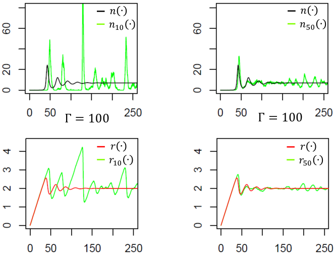
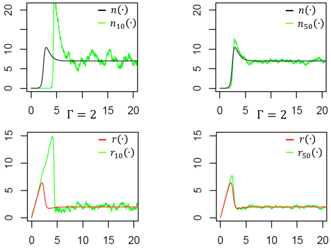
Behaviour of the empirical random density $X_{N}(t)$ for finite number of units $N$ is illustrated by Figures 1 and 2.

Figure 2: Dynamical system for $\Gamma=2$ : on the top the solution for $n$ (black), on the bottom for $r$ (red). Both starting at $0,01$. Trajectory samples of stochastic global Markov processes (green): for $N=10$ (top-left, bottom-left) and for $N=50$ (top-right, bottom-right), see definition (3.13). The chosen parameters are: $\alpha=0,01,\Gamma=2,P=7$ and $\beta=1$.

Remark 3.5.

Note that coefficients of transition intensities in $\mathbf{L}_{N}$ (3.2) are taken not from the driving dynamical system (3.11) for densities, but they are generating recursively, i.e., step-by-step along trajectories corresponding to the algorithm given by (3.2).

We also note that for jumps on $\Lambda_{N}=({1}/{\Gamma N})\mathbb{Z}_{+}\times({1}/{N})\mathbb{Z}_{+}$ the values of components of the Markov process $X_{N}(t)$ (3.13) are unbounded for any $N\geq 1$.

As we mentioned above the process $X_{N}(t)$ converges to a differentiable trajectory of DS (2.1), (2.2). The illustration of this statement is visible in Figures 1 ($\Gamma=100$) and Figure 2 ($\Gamma=2$), when one compares the realisations of $X_{N}(t)$ for $N=10$ and for $N=50$. The green trajectories get closer to the limit (3.14) for increasing $N$. Note that the spikes of the photon number for $n_{N=10}$ are more sound than in the case of $n_{N=50}$. Similarly, the fluctuations of the coefficient of inversion $r_{N=10}$ are more visible than those of $r_{N=50}$. Recall that these fluctuations are caused by fluctuations of the excited atoms with respect to the fixed number of non-excited atoms $N$.

Using this interpretation one can represent the total random number of excited atoms: $\xi_{N}(t)=Nr_{N}(t)$, and the random number of photons: $\eta_{N}(t)=Nn_{N}(t)$, as

$$\xi_{N}(t):=\sum_{j=1}^{N}\xi(t,j)\ \ {\rm{and}}\ \ \eta_{N}(t):=\sum_{j=1}^{N}\eta(t,j)\ .$$ (3.16)

Here for each index $j$: $1\leq j\leq N$, we introduce trajectories of identical, independent, compound unit-rate Poisson (telegraph) processes: $\{\xi(t,j)\}_{t\geq 0}$ with values $\xi(t,j)\in\{0,1\}$ for the jump-increment $1/\Gamma$, and $\{\eta(t,j)\}_{t\geq 0}$ with values $\eta(t,j)\in\{0,1\}$ for jump-increments equal to $1$.

Therefore, by (3.16) the density Markov process $X_{N}(t)$ (3.13) corresponds to empirical arithmetic means over trajectories: $\{\xi(t,j)\}_{t\geq 0,j=1,\ldots,N}$ and $\{\eta(t,j)\}_{t\geq 0,j=1,\ldots,N}$. Then the limit (3.14) expresses the LLN for the arithmetic means of (3.16) over parameter $N$ of the number of non-excited atoms.

3.3 Single Markov trajectories in a mean-field approximation

In this section instead of arithmetic means (3.16) corresponding to collective random variables $r_{N}(t)$ and $n_{N}(t)$ we consider the individual trajectories $\{\xi(t,j)\}_{t\geq 0}$ and $\{\eta(t,j)\}_{t\geq 0}$.

First we note that by virtue of (3.2) and the algorithm of calculations of transition intensities in Remark 3.5 besides the evident correlation between $\xi(t,j)$ and $\eta(t,j)$ for the same $j$, this trajectories are correlated since (3.2) is not a sum of independent generators $\{\mathbf{L}_{N}^{(j)}\}_{j=1,\ldots,N}$. To take into account the impact of these correlations on a single Markov trajectory $j$:

$$X_{N}^{(j)}(t):=\binom{{\xi(t,j)}}{{\eta(t,j)}}\ ,$$ (3.17)

we use a mean-field approximation. This approximation splits the above mentioned correlations and allows to present generator (3.2) as a sum generators for single trajectories correlated only in the mean-field.

To this aim we recall that coefficients of transitions in generator (3.2) are related to the instant values of density processes $x=r_{N}$ and $y=n_{N}$. Then one can use the representations: $Nr_{N}n_{N}=\frac{1}{2}\sum_{j=1}^{N}(x_{j}n_{N}+r_{N}y_{j})$, $Nr_{N}:=\sum_{j=1}^{N}x_{j}$, $Nn_{N}:=\sum_{j=1}^{N}y_{j}$, to rewrite $\mathbf{L}_{N}$ (3.2) identically in the form:

$$\mathbf{L}_{N}:=\sum_{j=1}^{N}\ \mathbf{\mathcal{L}}_{j}\ ,$$

where each $\mathbf{\mathcal{L}}_{j}$ represents generator of a singe trajectory correlated to others. In the mean-field approximation (which includes $n_{N}\approx n$ and $r_{N}\approx r$) we define generator $\mathbf{\mathcal{L}_{m-f}}$ for the single-trajectory (3.17) as:

$$(\mathbf{\mathcal{L}_{m-f}}\ g)\left(x,y\right) := \frac{1}{2}(x\,n+r\,y)[g(x-\frac{1}{\Gamma},y+1)-g(x,y)]$$

$$+ \alpha x[g(x-\frac{1}{\Gamma},y+1)-g(x,y)]$$

$$+ y[g(x+\frac{1}{\Gamma},y-1)-g(x,y)]$$

$$+ p[g(x+\frac{1}{\Gamma},y)-g(x,y)]$$

$$+ \beta^{-1}y[g(x,y-1)-g(x,y)]\ ,$$

for functions $g$ with compact supports on the lattice $\Lambda:=({1}/{\Gamma})\mathbb{Z}_{+}\times\mathbb{Z}_{+}$. Note that by equivalence of trajectories we skipped in (3.3) the index $j$, and that parameters $(r,n)$ are driven by the corresponding dynamical system for densities (3.11). Let denote a Markov process governed by the generator (3.3) by $Z(t)=(\xi(t),\eta(t))$.

Functions $r=r(t)$ and $n=n(t)$ appearing in the expression for the first rate in (3.3) depend on time following the evolution (3.11). But it is known that this dynamical system converges rapidly to the stationary point $(r^{*},n^{*})$ (2.4). Thus, in order to analyse the behaviour of the corresponding process it is reasonable to consider the Markov process, when the transition rates depend only on $(r^{*},n^{*})$. It makes the process homogeneous in time and facilitate the analysis. Denote such process by $Z_{0}(t)=(\xi_{0}(t),\eta_{0}(t))$. The following theorem states the ergodicity of the process.

Theorem 3.6.

If $\ {\Gamma}/{\beta}+{r^{*}}/{2}>1\$ the Markov process $Z_{0}(t)$ is positive recurrent (ergodic).

Proof. The proof is based on the construction of the Lyapunov function $f$ on the set of all state of Markov chain, such that the process $f(Z_{0}(t))$ will be super-martingale. To this aim we use the criterium of ergodicity from [7] (Theorem 1.7): In term of our process we have to find a non-negative function (Lyapunov function) $f(x,y)$ such that

$$(\mathbf{\mathcal{L}_{m-f}}\ f)\left(x,y\right)\leq-\varepsilon,$$

for some $\varepsilon>0$ and for all $(x,y)$ which do not belong to some finite subset $A$ (one must provide it) of the set of all state of the chain.

To this end let us define for our chain the following Lyapunov function :

$$f(x,y)=(\Gamma+1)x+y,\ \ \ x\in\frac{1}{\Gamma}\mathbb{Z}_{+},\ y\in\mathbb{Z}_{+}.$$ (3.19)

Then, applying the generator $\mathcal{L}_{m-f}$ to the Lyapunov function we obtain

$$(\mathbf{\mathcal{L}_{m-f}}\ f)\left(x,y\right) = -\frac{1}{\Gamma}\Bigl{(}\frac{xn^{*}+yr^{*}}{2}+\alpha x\Bigr{)}+\frac{1}{\Gamma}y+\frac{\Gamma+1}{\Gamma}p-\frac{y}{\beta}$$

$$= -\frac{1}{\Gamma}\Bigl{(}x\Bigl{(}\frac{n^{*}}{2}+\alpha\Bigr{)}+y\Bigl{(}\frac{\Gamma}{\beta}+\frac{r^{*}}{2}-1\Bigr{)}\Bigr{)}+\frac{\Gamma+1}{\Gamma}p\leq-\varepsilon\ ,$$

for some $\varepsilon>0$, when $xn^{*}+yr^{*}$ is sufficiently large. This provides the finite subset $A$, which is defined by

$$A:=\left\{(x,y)\in\frac{1}{\Gamma}\mathbb{Z}_{+}\times\mathbb{Z}_{+}:\frac{xn^{*}+yr^{*}}{2}+\alpha x+\Bigl{(}\frac{\Gamma}{\beta}-1\Bigr{)}y\leq(\Gamma+1)p+\Gamma\varepsilon\right\},$$

and consequently, completes the proof. $\Box$

Remark 3.7.

We note that ${\Gamma}/{\beta}+{r^{*}}/{2}>1$ is not a necessary condition. This choice of parameters makes the construction of Lyapunov function simple. We guess that the theorem holds true for any choice of positive parameters, $\Gamma,\beta$ and that it may be proved for other Lyapunov functions.

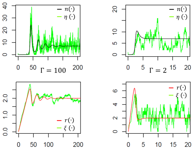
Behaviour of a single trajectories in the mean-field approximation is illustrated by Figure 3. Note that qualitatively it is more wiggling then the arithmetic mean for $N=50$, but less spiking then that for $N=10$, see Figures 1 and 2.

Figure 3: Dynamical system and mean-field trajectory: on the top, solutions for $n$ (black) $\Gamma=100$ and for $n$ (black) $\Gamma=2$; on the bottom, solutions for $r$ (red) $\Gamma=100$ and for $r$ (red) $\Gamma=2$. All starting at $0,01$. Single Markovian trajectories (green) in the mean-field approximation. On the top trajectory samples $\eta$ (green) for $\Gamma=100$ (left) and $\Gamma=2$ (right); on the bottom trajectory samples $\xi$ (green) for $\Gamma=100$ (left) and $\Gamma=2$ (right). All for parameters $\alpha=0,01,P=7,\beta=1$.

Taking into account the relation between representation (3.11) for DS and the form of generator (3.3) we deduce that corresponding to mean-field approximation dynamical system gets the form

$$\partial_{t}\binom{{r}}{{n}}=\Bigl{(}\frac{rn^{*}+nr^{*}}{2}+\alpha r\Bigr{)}\binom{-1/\Gamma}{1}+n\binom{1/\Gamma}{-1}+p\binom{1/\Gamma}{0}+\beta^{-1}n\binom{0}{-1}\ .$$ (3.20)

Then, in the stationary regime, we expect that its stationary points coincides with stationary points of DS. Indeed, the following theorem holds.

Theorem 3.8.

In the stationary regime, when $\partial_{t}{r}=\partial_{t}{n}=0$, (3.20) defines the stationary expectation values $(r^{**},n^{**})$ of the process $Z_{0}(t)=(\xi_{0}(t),\eta_{0}(t))$ which coincides with stationary points of DS $(r^{*},n^{*})$: $(r^{**},n^{**})=(r^{*},n^{*}).$

Proof. Since by (2.4)

$$\left\{\begin{array}[]{rcl}r^{*}&=&p(1+\beta)/(\beta p+\alpha)\ ,\\ n^{*}&=&\beta p\ ,\end{array}\right.$$

the explicit calculations with help of (3.20) yield $r^{**}=r^{*}$ and $n^{**}=n^{*}$. $\Box$

This confirms (at least for stationary regime) a consistency of expectations of $Z_{0}(t)=(\xi_{0}(t),\eta_{0}(t))$ for the process (3.3) with the values of $r^{*}$ and $n^{*}$ taken for the mean-field generator from DS (2.1), (2.2).

3.4 One-unit Markov process and spikes

In a sense we would like to study the case, which is intermediate between global ($N\gg 1$) and one-unit ($N=1$) limits. The one-unit Markov process describes the system for $N=1$. The corresponding generator (3.2) is simply $\mathbf{L}_{N=1}$:

$$(\mathbf{L_{1}}g)\left(x,y\right) = x\,y\ [g(x-\frac{1}{\Gamma},y+1)-g(x,y)]$$

$$+ \alpha x\ [g(x-\frac{1}{\Gamma},y+1)-g(x,y)]$$

$$+ y\ [g(x+\frac{1}{\Gamma},y-1)-g(x,y)]$$

$$+ p\ [g(x+\frac{1}{\Gamma},y)-g(x,y)]$$

$$+ \beta^{-1}y\ [g(x,y-1)-g(x,y)]\ ,$$

where we put $(r_{1},n_{1})=(x,y)\in\frac{1}{\Gamma}\mathbb{Z}_{+}\times\mathbb{Z}_{+}$

Figure 4: Markov processes for N=1. Top-left, bottom-left, the trajectory samples of stochastic Markov processes: $n_{1}$ (black) and $r_{1}$ (red), for the parameters $\alpha=0,01,\Gamma=100,P=7$ and $\beta=1$. Similarly, $n_{1}$ (black) and $r_{1}$ (red) on the top-right, bottom-right corresponds to parameters: $\alpha=0,01,\Gamma=2,P=7$ and $\beta=1$.

In this case the normalising parameter $N=1$ and we have only single Markov trajectory (3.17) $X_{N=1}(t){=\binom{r_{1}(t)}{n_{1}(t)}}$. Therefore, this is not a density dependent Markov process [3] driven by a dynamical system for densities.

According to (3.4) the first component $r_{1}(t)$ $\in({1}/{\Gamma})\mathbb{Z}_{+}$ of $X_{N=1}(t)$ is the random inversion coefficient, which is jumping between zero and infinity with increment $1/\Gamma$. The higher is excited level, the larger is the coefficient of inversion $\xi$ in the system. It is zero for the ground state of the system. On the other hand, the second component $n_{1}(t)$ $\in\mathbb{Z}_{+}$ of $X_{N=1}(t)$ is counting the instant number of photons in the system. It is also jumping between zero and infinity but with the increment one.

We note that interpretation of our model for $N=1$ is straightforward and perfectly understandable in the framework of Remark 3.1, when the total number: non-excited $+$ exited atoms is not fixed. But in fact it is also equivalent to a model with a single atom $N=1$. Indeed, since the coefficients of transition intensities in $\mathbf{L}_{1}$ are motivated by Einstein equations of Section 2.1, the one-unit system for $N=1$ allows interpretation as the model of a single infinitely-many level atom with the spacing between levels equals to $1/\Gamma$. This atom has the instant inversion coefficient $r_{1}$ and it is embedded into the random photon environment with the instant photon intensity $n_{1}$.

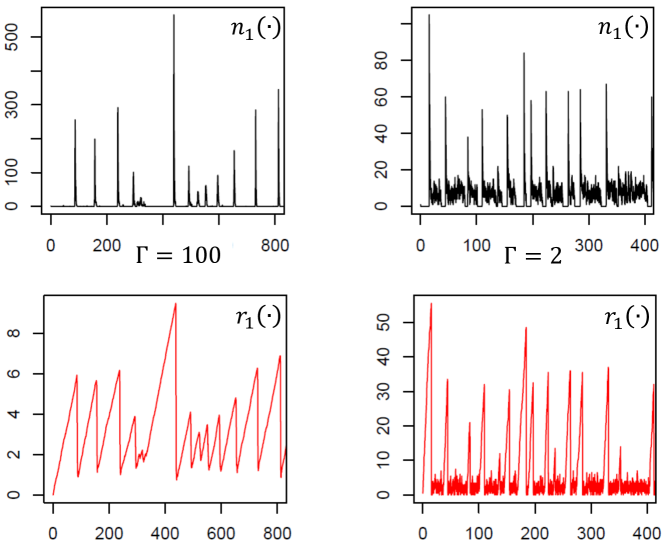
We illustrate the behaviour of the one-unit system on Figure 4.

Theorem 3.9.

When $\Gamma\geq\beta$ the Markov chain, which is governed by generator $\mathbf{L_{1}}$ is positive recurrent Markov chain.

Proof. The proof follows the same line of reasoning as above for individual component in mean-field. Moreover, the same Lyapunov function (3.19) can be applied in this case. Indeed, using (3.3) again we obtain

$$(\mathbf{L_{1}}f)\left(x,y\right)=-\frac{1}{\Gamma}\Bigl{(}xy+\alpha x+\Bigl{(}\frac{\Gamma}{\beta}-1\Bigr{)}y\Bigr{)}+\frac{\Gamma+1}{\Gamma}p\leq-\varepsilon$$ (3.22)

for some $\varepsilon>0$ and $x+y$ large enough, and when $\Gamma>\beta$. This also provides the set $A$ defined by:

$$A=\left\{(x,y):\ xy+\alpha x+\Bigl{(}\frac{\Gamma}{\beta}-1\Bigr{)}y\leq(\Gamma+1)p+\Gamma\varepsilon\right\}.$$

This gives the proof of assertion. $\Box$

3.5 One-unit process: statistics of spikes

The main characteristics of trajectory for $n_{1}(\cdot)$ in one-unit model is the presence of well featured spikes and plateaus just before spikes. Then a natural question concerns distributions of the spikes amplitude and of the lengths of plateau as well as their correlation. Since to obtain these distributions and correlation explicitly (analytically) is a difficult problem, we propose only some results of numerical statistical analysis.

Figure 5: Spikes amplitude statistics: Markov process for N=1, $\Gamma=100$ and $\Gamma=2$. Simulations were performed with the parameters: $\alpha=0,01,P=7$ and $\beta=1$. We see that the estimated tail probability follows the exponential law (middle column).

Figure 6: Plateau versus amplitude statistics: Markov process for one-unit process, $N=1$, $\Gamma=100$ and $\Gamma=2$. On the first and third scatterplots (for both $\Gamma=100$ and $\Gamma=2$) the plateau is defined as interval when $n_{1}(t)=0$. On the second and forth scatterplots the plateau is defined as the time interval when $n_{1}(t)\leq 10$ for the respectively ($\Gamma=100$ and $\Gamma=2$) same simulated trajectory. Other parameters in simulations were, as before, $\alpha=0,01,P=7$ and $\beta=1$.

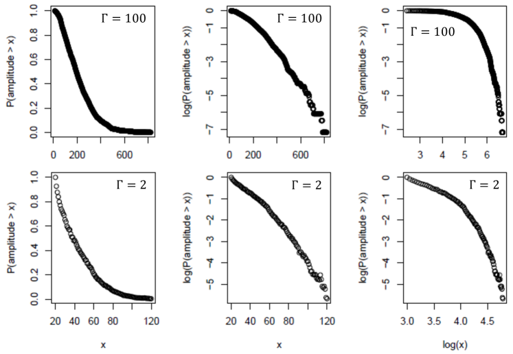
The statistics of spikes’ amplitudes for the one-unit Markov process with generator $\mathbf{L}_{1}$ is presented on the next Figure 5. On the simulated trajectory for a fixed value $a$ we calculate the frequency of times when the spikes are greater than $a$. For the case $\Gamma=100$ the minimal threshold for amplitude of spikes was chosen $a_{0}=10$, thus, we estimate the probability of the amplitude of spike greater than $a$ given the amplitude is greater then $10$. For $\Gamma=2$ the minimal threshold is $20$. These choice of minimal thresholds makes the graphs more readable. We observe in Figure 5 that the tail distribution of the amplitude in both cases ($\Gamma=100$ and $\Gamma=2$) is similar to exponential (median graphs).

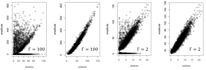
According the typical trajectories for the case when $\Gamma$ is large, see Figure 4 for $\Gamma=100$ we observe the presence of plateau (a time interval when $\eta(t)=0$). We expect that the plateau interval and a successive amplitude will be positively correlated. The first scatterplot, see the left hand-side scatterplot on Figure 6 gives us an idea about positive correlation between plateau and amplitude. But the figure also indicate the presence of large plateau with very small successive amplitude. It provide the new definition of plateau: a plateau is the time interval when $\eta(t)\leq thr$, where parameter $thr$ is threshold parameter. With new definition of plateau the tendency of positive correlation is more obvious, and moreover the dependency is not linear, which is illustrated for the case $\Gamma=100$ and $thr=10$ in right scatterplot on Figure 6.

It is instructive to compare the one-unit Markov process with generator $\mathbf{L}_{1}$ (3.4) with the single Markov trajectory in the mean-field approximation with generator $\mathbf{\mathcal{L}}$ (3.3). Note that only intensities of transitions in the first term are different. For the mean-field approximation the intensity is more smooth than for the one-unit Markov process, cf. the corresponding pictures Figure 3 and Figure 4.

Acknowledgements

This work was supported by Fundação de Amparo à Pesquisa do Estado de São Paulo (FAPESP) under Grant 2016/25077-4.

AY also thanks Conselho Nacional de Desenvolvimento Científico e Tecnolôgico (CNPq) grant 301050/2016-3 and FAPESP grant 2017/10555-0.

VAZ is grateful to Instituto de Matemática e Estatística of the University of São Paulo and to Anatoly Yambartsev for a warm hospitality. His visits were supported FAPESP grant 2016/25077-4.

References

- [1] Darling, R. W. R.; Norris, J. R. Differential equation approximations for Markov chains. Probability Surveys, 2008, 5, 37 - 79 .
- [2] Einstein, A. Zur Quantentheorie der Strahlung. Physikalische Zeitschrift, 1917, Bd.18, 121 - 128.
- [3] Ethier, S. N.; Kurtz, T. G. Markov processes: characterization and convergence. John Wiley & Sons, 2009, Vol. 282.
- [4] Jacod, J.; Shiryaev, A. N. Limit theorems for stochastic processes, vol.288 of Grundlehren der Mathematischen Wissenschaften. Springer-Verlag, Berlin, 2003.
- [5] Kolesnichenko, A. V.; Senni, V.; Pourranjabar, A.; Remke, A. K. I. Applying Mean-Field Approximation to Continuous Time Markov Chains. In: Stochastic Model Checking. Rigorous Dependability Analysis Using Model Checking Techniques for Stochastic Systems. Lecture Notes in Computer Science 8453. Springer Verlag, 2014, pp. 242-280.
- [6] Kurtz, T. G. Solutions of ordinary differential equations as limits of pure jump Markov processes. Journal of Applied Probability, 7(1), 49 - 58, 1970.
- [7] Menshikov, M.; Petritis, D. (2014). Explosion, implosion, and moments of passage times for continuous-time Markov chains: a semimartingale approach. Stochastic Processes and their Applications, 2014, 124(7), 2388-2414.
- [8] Renk, K. F. Basics of Laser Physics. Springer-Verlag, Berlin Heidelberg, 2012.