Knots in Physics

Abstract

After Dirac introduced the monopole, topological objects have played increasingly important roles in physics. In this review we discuss the role of the knot, the most sophisticated topological object in physics, and related topological objects in various areas in physics. In particular, we discuss how the knots appear in Maxwell’s theory, Skyrme theory, and multi-component condensed matter physics.

I Introduction

The topological objects have been assuming increasingly important roles in physics. The idea of topologically stable matter has first been proposed by Lord Kelvin more than a century ago, who suggested in 1868 that the atoms could be knots or links of vorticity lines of aether kelvin . When the topological stability of the knot was not well known in physics he understood that such knots and links would be extremely stable, just as matter is. This was a remarkable combination of geometric insight and physical intuition. The Kelvin’s idea was well received at that time, and praised (among others) by Maxwell.

Later in 1931, Dirac introduced one of the most important topological objects in physics, the Dirac monopole, which has the $\pi_{1}(S^{1})$ topology, the first homotopy of $S^{1}$ dirac . Based on this topology he proposed that the electric and magnetic charges $e$ and $g$ must satisfy the famous Dirac quantization rule $eg=2\pi n$, which explaines why the electric charge in nature has discrete values. Doing this he demonstrated, for the first time in human history, that topology can actually play a fundamental role in nature.

It was a remarkable coincidence that in the same year Hopf has shown that $S^{3}$ has the so-called Hopf fiberation $S^{2}\times S^{1}$, and that topologically $\pi_{3}(S^{2})$, the third homoptpy of $S^{2}$, can be classified by the Hopf index hopf ; bott . Mathematically this defines the knot topology and the knot number, which will play a crucial role in our discussion.

The Dirac monopole has changed the physics completely, and put the topology firmly in physics forever. Since then the monopole has become an obsession, theoretically and experimentally. Theoretically the non-Abelian monopoles based on $\pi_{2}(S^{2})$ topology, the singular Wu-Yang monopole in QCD wu ; prl80 and the regularized ’tHooft-Polyakov monopole in spontaneously broken gauge theory thooft ; dokos have been discovered. Experimentally huge efforts to discover the monopole have been made cab . But so far the search for the monopole has been unsuccessful, because the monopole which could exist in nature is not one of these monopoles but the electroweak monopole which is an hybrid between Dirac monopole and ’tHooft-Polyakov monopole plb97 ; yang .

In the mean time other interesting topological objects and their impacts in physics have become known. The Aharonov-Bohm effect and Berry phase are the well known examples of the impact of topology in physics bohm ; berry . But in 1961 Skyrme has pushed the topology to a new stage in physics sky . In his Skyrme theory he tried to realize the Kelvin’s dream proposing the proton (in general nuclei) to be the skyrmion, a topological soliton which has the $\pi_{3}(S^{3})$ topology. What is really remarkable is that he was proposing that we could construct fermions from bosons with the spin-isospin transmutation.

This view has become very successful from the theoretical point of view witt ; prep . A systematic method to construct multi-skyrmions with large baryon number based on the rational map was developed, which has allowed people to construct skyrmions with the baryon number up to 108 man ; bat ; sut ; sky108 . With this these multi-skyrmions have been identified with real nuclei.

In particular, the Skyrme theory could explain the spectrum of rotational excitations of carbon-12 and the Hoyle state successfully, which we need to generate heavy nuclear elements in early universe hoyle ; epel . In spite of these sucesses, the Skyrme’s proposal was too ideal to describe the real world.

Although the Skyrme theory was originally proposed as an effective theory for strong interaction, it has multiple faces which allow us to have totally different interpretations. First, it has many topologically interesting features and has all topological objects known in physics. In addition to the well known skyrmion, it has the (helical) baby skyrmion and the prototype knot known as the Faddeev-Niemi knot fadd ; prl01 . Most importantly, it has the monopole which plays the fundamental role. In fact the theory can be viewed as a theory of monopole which has a built-in Meissner effect, so that all finite energy topological objects in the theory could be viewed either as dressed monopoles or confined magnetic flux of the monopole-antimonopole pair prl01 ; plb04 ; ijmpa08 .

Of course, the fact that the skyrmion is closely related to the monopole has been noticed by many people. In spite of the fact that the skyrmions has been classified by the baryon number, people have used the rational map $\pi_{2}(S^{2})$ which describes the monopole number, not $\pi_{3}(S^{3})$ which describes the baryon number, to construct the multi-skyrmion solutions man . This strongly implies that the skyrmions can actually be viewed as the monopoles prl01 ; plb04 ; ijmpa08 . For this reason it has been proposed that the skyrmions carry two topological numbers, the baryon number and the monopole number epjc17 .

Furthermore, we can show that the Skyrme theory in fact has the multiple vacua which has the $\pi_{1}(S^{1})$ topology of the vacuum of Sine-Gordon theory and the $\pi_{3}(S^{2})$ topology of QCD vacuum combined together epjc17 . This means that the vacuum of the Skyrme theory can also be classified by two integers $(p,q)$, $p$ which represents the $\pi_{1}(S^{1})$ topology of the Sine-Gordon vacuum and $q$ which represents the $\pi_{3}(S^{2})$ topology of QCD. These new features demonstrates that the Skyrme theory has more topological features than we thought to have.

But what makes the Skyrme theory very important for the following discussion is that it can be reduced to the Skyrme-Faddeev theory which describes the prototype knot prl01 ; ijmpa08 . Moreover, we can derive the Skyrme-Faddeev theory which describes the core dynamics of the Skyrme theory directly from QCD.

Furthermore, we can argue that, with a simple modification the Skyrme theory could describe multi-gap superconductor or multi-component Bose-Einstein condensate which could contain the knot. This strongly indicates that the Skyrme theory could also be interpreted to describe a very interesting low energy condensed matter physics in a completely different environment. This puts the Skyrme theory in a totally new perspective.

It has long been believed that we need a complicated theory, in particular the non-Abelian structure or non-linear structure, to obtain the knot. This popular wisdom turned out to be totally wrong. In physics the knot was first discovered in Maxwell’s theory, a most unlikely place. In a series of paper in 1989 Ranada has shown that pure Maxwell’s theory without any electromagnetic source admits a wide class of propagating solitonic knot solutions he called “pseudo-photons,” generalizing Trautman’s work ran ; nat ; knotprep ; traut . This was surprizing.

Introducing two (electric and magnetic) complex scalars which is well defined at infinity, he constructed a set of propagating electromanetic knot solitons charactrized by two Hopf indices, the electric and magnetic helicity, which describe the Hopf map from the compactified space $S^{3}$ to the target space $S^{2}$. Moreover, he showed that this set of knot solutions is dense in the sense that a superposition of these topological solitions can describe, at least locally, any electromagnetic wave.

As importantly, in these set he showed that there is a natural mechanism for the quantization of electric charge by which the electric flux through any closed surface surrounding a singularity representing the electric charge becomes an integer. If this is true, the electromagnetic knots provides a new explanation of the topological charge quantization which is seemingly independent of the Dirac quantization rule. It would be very interesting to show if there is any relation between the two topological explanations of the charge quantization.

In his “daring conservatism”, Wheeler has conjectured the existence of “geons”, in particular the electromagnetic and gravitational geons, to propose that the elementary particles actually could be constructed from electromagnetic and/or gravitational fields and thus may not be so “elementary” wheel . But he could not show the existence of such geons. Ranada’s electromagnetic knots are the perfect examples of such geons. In particular, these knots acquire descrete masses in the absence of any mass scale in Maxwell’s theory, and thus demonstrate that the mass can be created from nothing.

This is really remarkable and astonishing. In QCD the mass can be created by the monopole condensation which generates the confinement prd13 ; prd15 . This is the dimensional transmutation in QCD. But here we have another example of dimensional transmutation, the mass from the energy, without any condensation or any new mechanism. This was what Wheeler visioned, and Ranada showed that this is possible. And at the center of this is the knot topology. It is the topology which makes it possible.

Mathematically the knot is defined as the mapping of a closed curve $S^{1}$ to a three-dimensinal space. The importance of this mapping is that this embedding can have non-trivial linking. Clearly this linking number does not change in any smooth deformation of the curve(s) and thus becomes a topological invariant. And in physics we often deal with curves; velocity curve, electric current, and magnetic flux. When they form closed curves, they may have non-vanishing linking number which does not change (i.e., is conserved) in dynamical evolotion, because it is a topological invariant. This is how the knot becomes important in physics.

Obviously this topological conservation applies to other topological objects as well, the magnetic monopoles and the skyrmions. And these days we can hardly talk about physics without mentioning these topological objects. Many of these topological objects are intimately related, but among them a most interesting object, mathematically as well as physically, is the knot hopf ; atiyah . And the knot appears everywhere in physics; in Maxwell’s electrodynamics ran ; berry1 , Skyrme theory prl01 ; plb04 ; ijmpa08 , QCD plb05 , fluid dynamics moff , atomic physics berry2 ; pra05 , plasma physics berg , polymer physics kami , condensed matter physics baba ; prb06 ; epjb08 , even in Einstein’s theory cqg13 .

The purpose of this paper is to review the role of the knots and related topological objects, in particular the monopoles and skyrmions, in physics and to discuss their importance. Although the knot appears in all area of physics, we will discuss the knot in Skyrme theory in detail because the Skyrme theory is a best place to discuss the topological objects in physics.

The paper is organized as follows. In Section II we discuss the Ranada’s construction of the electromagnetic knot and its physical implication. In Section III we review the Skyrme theory, and show that the core dynamics of the theory is described by the Skyrme-Faddeev theory which has the non-Abelian monopole and the prototype knot. In Section IV we show that the Skyrme-Faddeev theory can actually be derived from the SU(2) QCD, and discuss a deep connection between the two theories. In Section V we discuss two types of topology in skyrmions, and show that skyrmions actually carry two different topology, the $\pi_{2}(S^{2})$ topology of the monopole as well as the well known $\pi_{3}(S^{3})$ topology of skyrmion. In Section VI we discuss the vacuum structure of Skyrme theory, and show that it has the multiple vacua made of the vacuum topology of Sine-Gordon theory and QCD combined together. In Section VII we review the prototype knot in Skyrme theory which can be viewed as the twisted magnetic vortex ring made of the monopole-antimonopole pair. In Section VIII we show how similar knots could appear in condensed matter physics, in particular in multi-gap superconductors and multi-component Bose-Einstein condensate. Finally in the last section we discuss the physical implications of the knots.

II Knots in Maxwell’s Theory

Maxwell’s theory has played fundamental role in physics. In spite of the mathematical beauty and the huge practical applications, however, the theory has been thought to be too simple to admit topological objects. Of course, Dirac showed us that it can be generalized to allow the U(1) monopole structure, but as far as topology is concerned this was all. Fortunately this general wisdom turned out to be completely wrong.

In fact the Maxwell’s theory, without Dirac’s generalization, has very interesting knots ran . But this important topological feature of Maxwell’s theory so far has not been well known, because people believed that the theory, being linear, has no structure for topological object. So we discuss the knots in Maxwell’s theory first.

To understand how this could be possible, notice that the electric and magnetic field lines could form closed loops and thus be linked, and this linking could provide the topological structure. Let two closed field lines be $\vec{c}_{1}(s)$ and $\vec{c}_{2}(s)$. They are linked if they have a non-vanishing Gauss integral,

$$L(\vec{c}_{1},\vec{c}_{2})=\dfrac{1}{4\pi}{\displaystyle\int}\Big{(}\dfrac{\vec{c}_{1}-\vec{c}_{2}}{|\vec{c}_{1}-\vec{c}_{2}|^{3}}\times\dfrac{\vec{c}_{1}}{ds_{1}}\Big{)}\cdot\dfrac{\vec{c}_{2}}{ds_{2}}ds_{1}ds_{2},$$ (1)

where the self-linking number $L(\vec{c},\vec{c})$ describes the knottedness. In the case of the electric and magnetic fields the average of the the linking integral over all field line pairs together with the self-linking number over all field lines give rise to the electric and magnetic helicities given by the Chern-Simon integrals,

$$h_{e}={\displaystyle\int}\epsilon_{ijk}C_{i}(\partial_{j}C_{j}-\partial_{k}C_{j})~{}d^{3}x,$$

$$h_{m}={\displaystyle\int}\epsilon_{ijk}A_{i}(\partial_{j}A_{j}-\partial_{k}A_{j})~{}d^{3}x.$$ (2)

Here $C_{i}$ and $A_{i}$ are the vector potentials of the electric and magnetic field, which exist in free Maxwell’s theory. And in Maxwell’s theory these integer helicities determine the $\pi_{3}(S^{2})$ topology of the electromagnetic knots.

To explain this in more detail we first construct the electromagnetic knot. Let $\zeta$ and $\eta$ be two complex scalar fields representing the map from the space-time $R^{3}\times T$ to the complex plane $R^{2}$. Compactifying $R^{3}$ and $R^{2}$ to $S^{3}$ and $S^{2}$ with the streographic projection, we can view that the two complex fields define the map from $S^{3}$ to $S^{2}$ which can be classified by the knot topology $\pi_{3}(S^{2})$.

Next, we define two anti-symmetric electromagnetic tensor fields $F_{\mu\nu}$ and $H_{\mu\nu}$ by

$$F_{\mu\nu}=\dfrac{\sqrt{\alpha}}{2\pi i}\times\dfrac{\partial_{\mu}\zeta^{*}\partial_{\nu}\zeta-\partial_{\nu}\zeta^{*}\partial_{\mu}\zeta}{(1+\zeta^{*}\zeta)^{2}},$$

$$H_{\mu\nu}=\dfrac{\sqrt{\alpha}}{2\pi i}\times\dfrac{\partial_{\mu}\eta^{*}\partial_{\nu}\eta-\partial_{\nu}\eta^{*}\partial_{\mu}\eta}{(1+\eta^{*}\eta)^{2}},$$ (3)

where we have put an action constant $\alpha$ to make the tensor fields to have the dimension of the electromagnetic fields. We further require $F_{\mu\nu}$ and $H_{\mu\nu}$ to be dual to each other,

$$F_{\mu\nu}=\dfrac{1}{2}\epsilon_{{\mu\nu}{\alpha\beta}}H^{\alpha\beta},~{}~{}~{}H_{\mu\nu}=-\dfrac{1}{2}\epsilon_{{\mu\nu}{\alpha\beta}}F^{\alpha\beta}.$$ (4)

Now we can prove that, if $\zeta$ and $\eta$ satisfy the equation

$$\partial_{\mu}F^{{\mu\nu}}\partial_{\nu}\zeta=0,~{}~{}~{}\partial_{\mu}F^{{\mu\nu}}\partial_{\nu}\zeta^{*}=0,$$

$$\partial_{\mu}H^{{\mu\nu}}\partial_{\nu}\eta=0,~{}~{}~{}\partial_{\mu}H^{{\mu\nu}}\partial_{\nu}\eta^{*}=0,$$ (5)

$F_{\mu\nu}$ and $H_{\mu\nu}$ become the solutions of Maxwell’s equation, and thus describe the electromagnetic fields ran .

Notice that (5) tells that, if the Cauchy data $(\zeta,\dot{\zeta},\eta,\dot{\eta})$ at $t=0$ satisfies the duality condition (4), it does so for all $t$. Moreover, (3) assures that $F_{\mu\nu}$ and $H_{\mu\nu}$ satisfy the first half of Maxwell’s equation

$$\epsilon_{{\mu\nu}{\alpha\beta}}\partial^{\nu}F^{\alpha\beta}=0,~{}~{}~{}\epsilon_{{\mu\nu}{\alpha\beta}}\partial^{\nu}H^{\alpha\beta}=0,$$ (6)

independent of $\zeta$ and $\eta$. Besides, this together with the duality condition (4) assures that they satisfy the second half of Maxwell’s equation

$$\partial_{\mu}F^{\mu\nu}=0,~{}~{}~{}\partial_{\mu}H^{\mu\nu}=0.$$ (7)

So $F_{\mu\nu}$ and $H_{\mu\nu}$ become solutions of Maxwell’s theory. The important point here is that these solutions are encoded by the electric and magnetic helicities of the $\pi_{3}(S^{2})$ topology given by $\zeta$ and $\eta$.

A few comments are in order. First, (3) tells that $\vec{E}(\zeta)$ and $\vec{B}(\zeta)$ are mutually orthogonal. Moreover, $\vec{B}(\zeta)$ and $\vec{B}(\eta)$ are tangent to the curve $\zeta=const$ and $\eta=const$. So the two fields $\vec{E}$ and $\vec{B}$ are orthogonal to each other ($\vec{E}\cdot\vec{B}=0$), and the solutions represent the radiational wave. Second, although we have introduced two complex scalar fields $\zeta$ and $\eta$, it must be clear that only one is indepent. This is because $F_{\mu\nu}$ and $H_{\mu\nu}$ are dual to each other.

To find the solutions, we have to solve (5). This is a non-trivial task. So, in stead of solving the equations, Ranada constructed what he called an admissible set of solutions classified by two Hoph numbers, the electric and magnetic helicities, by judiciously choosing $\zeta$ which describes the Hopf map.

Consider the map proposed by Hopf hopf

$$\phi_{H}=\frac{2(x+iy)}{2z+i(r^{2}-1)},~{}~{}~{}(r^{2}=x^{2}+y^{2}+z^{2}).$$ (8)

Notice that any two level curves of this mapping, for example the curve $\phi_{H}=0$ and the curve $\phi_{H}=\infty$, are linked once. So the mapping defines the $\pi_{3}(S^{2})$ map with Hopf index one. Now, let us define $\zeta$ and $\eta$ by

$$\zeta=\phi_{H}(\kappa y,\kappa z,\kappa x),~{}~{}~{}\eta=\phi_{H}^{*}(\kappa z,\kappa x,\kappa y),$$ (9)

where $\kappa$ is a dimensional parameter with dimension of mass (inverse length). Then we can easily check the electromagnetic field given by (3) satisfies the Maxwell’s equation which has $h_{e}=h_{m}=1$. This solution is called the electromagnetic knot ran .

The energy, momentum, and angular momentum of this solution can be computed from the energy density, momentum density, and angular momentum density, $(\vec{E}^{2}+\vec{B}^{2})/2$, $\vec{E}\times\vec{B}$, and $\vec{x}\times(\vec{E}\times\vec{B})$. They are given by

$$E=2\kappa,~{}~{}~{}\vec{p}=(0,0,\kappa),~{}~{}~{}\vec{J}=(0,0,1).$$ (10)

The solution describes a wavepacket given by the potential (with $A_{0}=0$)

$$\vec{A}=\frac{\kappa^{2}}{(2\pi)^{3/2}}{\displaystyle\int}\frac{1}{\omega}\Big{[}\vec{R}_{2}(\vec{k})\cos(\vec{k}\cdot\vec{r}-\omega t)$$

$$+\vec{R}_{1}(\vec{k})\sin(\vec{k}\cdot\vec{r}-\omega t)\Big{]}d^{3}k,$$

$$\vec{R}_{1}=\frac{\exp(-\omega/\kappa)}{(2\pi)^{1/2}\kappa}\Big{(}-\frac{k_{1}k_{3}}{\omega},\frac{k_{2}^{2}+k_{3}^{2}}{\omega}+k_{2},$$

$$-\frac{k_{1}k_{2}}{\omega}-k_{1}\Big{)},$$

$$\vec{R}_{2}=\frac{\exp(-\omega/\kappa)}{(2\pi)^{1/2}\kappa}\Big{(}-\frac{k_{1}^{2}+k_{2}^{2}}{\omega}-k_{2},$$

$$\frac{k_{1}k_{3}}{\omega},\frac{k_{2}k_{3}}{\omega}+k_{3}\Big{)},$$ (11)

traveling along the $z$-axis with velocity $p/E=1/2$ which has the electromagnetic field given by

$$\vec{E}=\frac{\kappa^{2}}{(2\pi)^{3/2}}{\displaystyle\int}\Big{[}\vec{R}_{1}(\vec{k})\cos(\vec{k}\cdot\vec{r}-\omega t)$$

$$-\vec{R}_{2}(\vec{k})\sin(\vec{k}\cdot\vec{r}-\omega t)\Big{]}d^{3}k,$$

$$\vec{B}=\frac{\kappa^{2}}{(2\pi)^{3/2}}{\displaystyle\int}\Big{[}\vec{R}_{2}(\vec{k})\cos(\vec{k}\cdot\vec{r}-\omega t)$$

$$+\vec{R}_{1}(\vec{k})\sin(\vec{k}\cdot\vec{r}-\omega t)\Big{]}d^{3}k.$$ (12)

Notice that this wavepacket has the mass $m^{2}=E^{2}-{\vec{p}}^{2}=3\kappa^{2}$. Clearly this is the electromagnetic geon visioned by Wheeler. The fact that we have such topologically stable finite energy solitonic solutions in Maxwell’s theory is really remarkable.

Ranada showed that one can construct a whole set of knot solutions with arbitrary integer helicities ran . Moreover, he showed that this set is dense, in the sense that we can construct any radiational wave superposing them, at least locally.

What is more remarkable is that in this formalism the electric charge has to be quantized. Introducing a point singularity which represents the electric charge in these solutions he showed that the total charge, i.e., the integral of the outgoing electric flux over the closed surface surrounding the singularity, must be quantized and have discrete values. This is basically because these point singularities aquires the $\pi_{2}(S^{2})$ topology which necessitates the electric charge quantization ran . Notice that here the $\pi_{2}(S^{2})$ topology describes the electric, not magnetic, charge. Doing so, he has found another reason why the electric charge in nature is quantized. This is really remarkable because here we do not have to assume the existence of the monopole to have the electric charge quantization.

Certainly the electromagnetic knots are very interesting from the theoretical point of view. As importantly, they have huge potential applications in many area, from colloidal and atomic particle trapping to the plasma confinement nat . But we have to keep in mind that, unlike other known topological objects in physics, the electromagnetic knot has a non-trivial time dependence.

III Skyrme Theory: A Review

The Skyrme theory has played an important role in physics. Originally it was proposed as a theory of pion physics in strong interaction where the skyrmion, a topological soliton made of pions, appears as the baryon sky . Soon after, the theory has been interpreted as a low energy effective theory of QCD in which the massless pion fields emerge as the Nambu-Goldstone boson of the spontaneous chiral symmetry breaking witt ; prep . This view has become popular and very successful, as we have already mentioned man ; bat ; sut ; sky108 ; hoyle ; epel .

But the Skyrme theory has multiple faces and has other topologically interesting objects. In fact we can say that the theory has all topological objects known in physics. In addition to the well known skyrmion which has the $\pi_{3}(S^{3})$ topology it has the baby skyrmion which has the $\pi_{1}(S^{1})$ topology, the monopole which has the $\pi_{2}(S^{2})$ topology, and the knot which has the $\pi_{3}(S^{2})$ topology.

Among these the monopole plays the fundamental role. The central piece of the theory is the singular Wu-Yang type monopole which makes up all topological objects in the theory. Indeed, the skyrmion can be viewed as a finite energy dressed monopole, the baby skyrmion as a magnetic vortex connecting the monopole-antimonopole pair, and the knot as a twisted magnetic vortex ring made of the helical baby skyrmion. So the theory can be viewed as a theory of monopole which has a built-in Meissner effect prl01 ; plb04 ; ijmpa08 .

Moreover, the Skyrme theory has the multiple vacua similar to the Sine-Gordon theory, each of which has the knot topology of the QCD vacuum epjc17 . In other words, the vacuum of the Skyrme theory has the topology of the Sine-Gordon theory and QCD combined together. So, the vacuum of the Skyrme theory can also be classified by two integers by $(p,q)$, $p$ which represents the $\pi_{1}(S^{1})$ topology and $q$ which represents the $\pi_{3}(S^{2})$ topology.

It has been appreciated for a long time that the skyrmion is described by the monopole topology. But since the monopole topology $\pi_{2}(S^{2})$ and the baryon topology $\pi_{3}(S^{3})$ are different, the skyrmions should be classified by two topological numbers, the baryon number $b$ and the monopole number $m$ epjc17 . According to this view the baryon number can also be replaced by the radial (shell) quantum number $n$ which describes the $\pi_{1}(S^{1})$ topology of the radial extension of the skyrmions. This is based on the observation that the $S^{3}$ space (both the compactified 3-dimensional real space and the SU(2) target space) has the Hopf fibering $S^{3}\simeq S^{2}\times S^{1}$, so that the baryon number defined by $\pi_{3}(S^{3})$ can be decomposed to two topological numbers $\pi_{2}(S^{2})$ and $\pi_{1}(S^{1})$.

The fact that the skyrmions have two topology can be extended to the baby skyrmion. We can construct new solutions of baby skyrmion, and show that they have two topology, the shell (radial) topology $\pi_{1}(S^{1})$ and the monopole topology $\pi_{2}(S^{2})$. This is really remarkable, which strongly support that the skyrmion does carry two topology. These unique features make the Skyrme theory an ideal place for us to discuss the topology in physics.

We first review the well known facts in Skyrme theory. Let $\omega$ and $\hat{n}$ (${\hat{n}}^{2}=1$) be the massless scalar field (the “sigma-field”) and the normalized pion-field in Skyrme theory, and write the Skyrme Lagrangian as sky

$${\cal L}=\dfrac{\kappa^{2}}{4}{\rm tr}~{}L_{\mu}^{2}+\dfrac{\alpha}{32}{\rm tr}\left(\left[L_{\mu},L_{\nu}\right]\right)^{2}$$

$$=-\dfrac{\kappa^{2}}{4}\Big{[}\dfrac{1}{2}(\partial_{\mu}\omega)^{2}+2\sin^{2}\dfrac{\omega}{2}(\partial_{\mu}\hat{n})^{2}\Big{]}$$

$$-\dfrac{\alpha}{8}\Big{[}\sin^{2}\dfrac{\omega}{2}\big{(}(\partial_{\mu}\omega)^{2}(\partial_{\nu}\hat{n})^{2}-(\partial_{\mu}\omega\partial_{\nu}\omega)(\partial_{\mu}\hat{n}\cdot\partial_{\nu}\hat{n})\big{)}$$

$$+2\sin^{4}\dfrac{\omega}{2}(\partial_{\mu}\hat{n}\times\partial_{\nu}\hat{n})^{2}\Big{]},$$

$$L_{\mu}=U\partial_{\mu}U^{\dagger},$$

$$U=\exp(\dfrac{\omega}{2i}\vec{\sigma}\cdot\hat{n})=\cos\dfrac{\omega}{2}-i(\vec{\sigma}\cdot\hat{n})\sin\dfrac{\omega}{2},$$ (13)

where $\kappa$ and $\alpha$ are the coupling constants.

Notice that, with

$$\sigma=\cos\dfrac{\omega}{2},~{}~{}~{}\vec{\pi}=\hat{n}\sin\dfrac{\omega}{2},~{}~{}~{}(\sigma^{2}+\vec{\pi}^{2}=1),$$ (14)

the Lagrangian (13) can also be put into the form

$${\cal L}=-\dfrac{\kappa^{2}}{2}\big{(}(\partial_{\mu}\sigma)^{2}+(\partial_{\mu}\vec{\pi})^{2}\big{)}$$

$$-\dfrac{\alpha}{4}\big{(}(\partial_{\mu}\sigma\partial_{\nu}\vec{\pi}-\partial_{\nu}\sigma\partial_{\mu}\vec{\pi})^{2}+(\partial_{\mu}\vec{\pi}\times\partial_{\nu}\vec{\pi})^{2}\big{)}$$

$$+\dfrac{\lambda}{4}(\sigma^{2}+\vec{\pi}^{2}-1),$$ (15)

where $\lambda$ is a Lagrange multiplier. In this form $\sigma$ and $\vec{\pi}$ represent the sigma field and the pion field, so that the theory describes the non-linear sigma model of the pion physics.

The Lagrangian has a hidden $U(1)$ gauge symmetry as well as the global $SU(2)_{L}\times SU(2)_{R}$ symmetry plb04 ; ijmpa08 . The global $SU(2)_{L}\times SU(2)_{R}$ symmetry is obvious, but the hidden $U(1)$ gauge symmetry is not. The hidden $U(1)$ gauge symmetry comes from the $U(1)$ subgroup which leaves $\hat{n}$ invariant. To see this, we reparametrize $\hat{n}$ by the $CP^{1}$ field $\xi$,

$$\hat{n}=\xi^{\dagger}\vec{\sigma}\xi,~{}~{}~{}~{}~{}\xi^{\dagger}\xi=1.$$ (16)

and find that under the $U(1)$ gauge transformation of $\xi$ to

$$\xi\rightarrow\exp(i\theta(x))\xi,$$ (17)

$\hat{n}$ (and $\partial_{\mu}\hat{n}$) remains invariant. Now, we introduce the composite gauge potential $C_{\mu}$ and the covariant derivative $D_{\mu}$ which transforms gauge covariantly under (17) by

$$C_{\mu}=-2i\xi^{\dagger}\partial_{\mu}\xi,~{}~{}~{}D_{\mu}\xi=(\partial_{\mu}-\frac{i}{2}C_{\mu})\xi.$$ (18)

With this we have the following identities,

$$(\partial_{\mu}\hat{n})^{2}=4|D_{\mu}\xi|^{2},$$

$$\partial_{\mu}\hat{n}\times\partial_{\nu}\hat{n}=-2i\Big{[}(\partial_{\mu}\xi^{\dagger})(\partial_{\nu}\xi)-(\partial_{\mu}\xi^{\dagger})(\partial_{\nu}\xi)\Big{]}\hat{n}$$

$$=H_{\mu\nu}\hat{n},$$

$$H_{\mu\nu}=\partial_{\mu}C_{\nu}-\partial_{\nu}C_{\mu}.$$ (19)

Furthermore, with the Fierz’ identity

$$\sigma_{ij}^{a}\sigma_{kl}^{a}=2\delta_{il}\delta_{jk}-\delta_{ij}\delta_{kl},$$ (20)

we have

$$\partial_{\mu}\hat{n}\cdot\partial_{\mu}\hat{n}=2\partial_{\mu}(\xi^{\dagger}_{i}\xi_{j})\partial_{\nu}(\xi^{\dagger}_{j}\xi_{i})$$

$$=2\Big{[}(\partial_{\mu}\xi^{\dagger}\xi)(\partial_{\nu}\xi^{\dagger}\xi)+(\partial_{\mu}\xi^{\dagger})(\partial_{\nu}\xi)+(\partial_{\nu}\xi^{\dagger})(\partial_{\mu}\xi)$$

$$+(\xi^{\dagger}\partial_{\mu}\xi)(\xi^{\dagger}\partial_{\nu}\xi)\Big{]}=2\Big{[}(\partial_{\mu}\xi^{\dagger}+\frac{i}{2}C_{\mu}\xi^{\dagger})(\partial_{\nu}\xi-\frac{i}{2}C_{\nu}\xi)$$

$$+(\partial_{\nu}\xi^{\dagger}+\frac{i}{2}C_{\nu}\xi^{\dagger})(\partial_{\mu}\xi-\frac{i}{2}C_{\mu}\xi)\Big{]}$$

$$=2\Big{[}(D_{\mu}\xi)^{\dagger}(D_{\nu}\xi)+(D_{\nu}\xi)^{\dagger}(D_{\mu}\xi)\Big{]}.$$ (21)

From this we can express (13) by

$${\cal L}=-\dfrac{\kappa^{2}}{4}\Big{[}\dfrac{1}{2}(\partial_{\mu}\omega)^{2}+8\sin^{2}\dfrac{\omega}{2}|D_{\mu}\xi|^{2}\Big{]}$$

$$-\dfrac{\alpha}{2}\sin^{2}\dfrac{\omega}{2}\Big{[}(\partial_{\mu}\omega)^{2}|D_{\mu}\xi|^{2}-(\partial_{\mu}\omega\partial_{\nu}\omega)(D_{\mu}\xi)^{\dagger}(D_{\nu}\xi)$$

$$+\frac{1}{2}\sin^{2}\dfrac{\omega}{2}H_{\mu\nu}^{2}\Big{]},$$ (22)

which is explicitly invariant under the $U(1)$ gauge transformation (17). So replacing $\hat{n}$ by $\xi$ in the Lagrangian we can make the hidden $U(1)$ gauge symmetry explicit. In this form the Skyrme theory becomes a self-interacting $U(1)$ gauge theory of $CP^{1}$ field coupled to a massless scalar field.

The equations of motion of the Lagrangian is given by

$$\partial^{2}\omega-\sin\omega(\partial_{\mu}\hat{n})^{2}+\dfrac{\alpha}{8\kappa^{2}}\sin\omega(\partial_{\mu}\omega\partial_{\nu}\hat{n}-\partial_{\nu}\omega\partial_{\mu}\hat{n})^{2}$$

$$+\dfrac{\alpha}{\kappa^{2}}\sin^{2}\dfrac{\omega}{2}\partial_{\mu}\big{[}(\partial_{\mu}\omega\partial_{\nu}\hat{n}-\partial_{\nu}\omega\partial_{\mu}\hat{n})\cdot\partial_{\nu}\hat{n}\big{]}$$

$$-\dfrac{\alpha}{\kappa^{2}}\sin^{2}\dfrac{\omega}{2}\sin\omega(\partial_{\mu}\hat{n}\times\partial_{\nu}\hat{n})^{2}=0,$$

$$\partial_{\mu}\Big{\{}\sin^{2}\dfrac{\omega}{2}\hat{n}\times\partial_{\mu}\hat{n}+\dfrac{\alpha}{4\kappa^{2}}\sin^{2}\dfrac{\omega}{2}\big{[}(\partial_{\nu}\omega)^{2}\hat{n}\times\partial_{\mu}\hat{n}$$

$$-(\partial_{\mu}\omega\partial_{\nu}\omega)\hat{n}\times\partial_{\nu}\hat{n}\big{]}$$

$$+\dfrac{\alpha}{\kappa^{2}}\sin^{4}\dfrac{\omega}{2}(\hat{n}\cdot\partial_{\mu}\hat{n}\times\partial_{\nu}\hat{n})\partial_{\nu}\hat{n}\Big{\}}=0.$$ (23)

Clearly the second equation describes the conservation of $SU(2)$ current originating from the global $SU(2)$ symmetry of the theory.

It has two interesting limits. First, when

$$\omega=(2p+1)\pi,$$ (24)

(23) is reduced to

$$\hat{n}\times\partial^{2}\hat{n}-\dfrac{\alpha}{\kappa^{2}}(\partial_{\mu}H_{\mu\nu})\partial_{\nu}\hat{n}=0,$$

$$H_{\mu\nu}=\hat{n}\cdot(\partial_{\mu}\hat{n}\times\partial_{\nu}\hat{n})=\partial_{\mu}C_{\nu}-\partial_{\nu}C_{\mu},$$ (25)

where $C_{\mu}$ is the magnetic potential of $H_{\mu\nu}$ defined by (18). This is the central equation of Skyrme theory which allows the monopole, the baby skyrmion, and the Faddeev-Niemi knot prl01 ; plb04 ; ijmpa08 .

Second, in the spherically symmetric limit

$$\omega=\omega(r),~{}~{}~{}~{}~{}\hat{n}=\pm\hat{r},$$ (26)

(23) is reduced to

$$\dfrac{d^{2}\omega}{dr^{2}}+\dfrac{2}{r}\dfrac{d\omega}{dr}-\dfrac{2\sin\omega}{r^{2}}+\dfrac{2\alpha}{\kappa^{2}}\Big{[}\dfrac{\sin^{2}(\omega/2)}{r^{2}}\dfrac{d^{2}\omega}{dr^{2}}$$

$$+\dfrac{\sin\omega}{4r^{2}}(\dfrac{d\omega}{dr})^{2}-\dfrac{\sin\omega\sin^{2}(\omega/2)}{r^{4}}\Big{]}=0.$$ (27)

This is the equation used by Skyrme to find the original skyrmion. Imposing the boundary condition

$$\omega(0)=2\pi,~{}~{}~{}~{}~{}\omega(\infty)=0,$$ (28)

we have the skyrmion solution which carries the unit baryon number sky

$$B=-\dfrac{1}{24\pi^{2}}{\displaystyle\int}\epsilon_{ijk}~{}{\rm tr}~{}(L_{i}L_{j}L_{k})d^{3}r$$

$$=-\dfrac{1}{8\pi^{2}}\int\epsilon_{ijk}\partial_{i}\omega\big{[}\hat{r}\cdot(\partial_{j}\hat{r}\times\partial_{k}\hat{r})\big{]}\sin^{2}\dfrac{\omega}{2}d^{3}r$$

$$=1,$$ (29)

which represents the non-trivial homotopy $\pi_{3}(S^{3})$ defined by $U$.

The two limits lead us to very interesting physics. To understand the physical meaning of the first limit notice that, with (24) the Skyrme Lagrangian reduces to the Skyrme-Faddeev Lagrangian

$${\cal L}\rightarrow-\dfrac{\kappa^{2}}{2}(\partial_{\mu}\hat{n})^{2}-\dfrac{\alpha}{4}(\partial_{\mu}\hat{n}\times\partial_{\nu}\hat{n})^{2},$$ (30)

whose equation of motion is given by (25). This tells that the Skyrme-Faddeev theory becomes a self-consistent truncation of the Skyrme theory. This assures that the Skyrme-Faddeev theory is an essential ingredient (the backbone) of the Skyrme theory which describes the core dynamics of Skyrme theory prl01 ; plb04 ; ijmpa08 .

A remarkable feature of the Skyrme-Faddeev theory is that it can be viewed as a theory of monopole. In fact, (25) has the singular monopole solution prl01 ; plb04 ; ijmpa08

$$\hat{n}=\pm\hat{r}.$$ (31)

which carries the magnetic charge

$$Q_{m}=\dfrac{\pm 1}{8\pi}\int\epsilon_{ijk}\big{[}\hat{r}\cdot(\partial_{i}\hat{r}\times\partial_{j}\hat{r})\big{]}d\sigma_{k}=\pm 1,$$ (32)

which represents the homotopy $\pi_{2}(S^{2})$ defined by $\hat{n}$. Of course, (31) has a point singularity at the origin which makes the energy divergent. But we can easily regularize the singularity with a non-trivial $\omega$, with the boundary condition (28). And the regularized monopole becomes nothing but the well known skyrmion.

Moreover, it has the (helical) magnetic vortex solution made of the monopole-antimonopole pair infinitely separated apart, and the knot solution which can be viewed as the twisted magnetic vortex ring made of the helical vortex whose periodic ends are connected together. So the monopole plays an essential role in all these solutions. This shows that the Skyrme-Faddeev theory, and by implication the Skyrme theory itself, can be viewed as a theory of monopole.

But perhaps a most important point of the Skyrme-Faddeev Lagrangian is that it provides a “missing” link between Skyrme theory and QCD, because the Skyrme-Faddeev Lagrangian can actually be derived from QCD prl01 ; plb04 ; ijmpa08 .

IV Skyrme Theory and QCD: A Theory of Monopole

To reveal the deep connection between Skyrme theory and QCD, consider the SU(2) QCD

$${\cal L}_{QCD}=-\dfrac{1}{4}\vec{F}_{\mu\nu}^{2}.$$ (33)

Now, we can make the Abelian projection choosing the Abelian direction to be $\hat{n}$ and imposing the Abelian isometry

$$D_{\mu}\hat{n}=0,$$ (34)

to the gauge potential. With this we obtain the restricted potential $\hat{A}_{\mu}$ which describes the color neutral binding gluon (the neuron) prd80 ; prl81

$${\vec{A}}_{\mu}\rightarrow\hat{A}_{\mu}={\cal A}_{\mu}+{\cal C}_{\mu},$$

$${\cal A}_{\mu}=A_{\mu}\hat{n},~{}~{}~{}{\cal C}_{\mu}=-\dfrac{1}{g}\hat{n}\times\partial_{\mu}\hat{n}.$$ (35)

The restricted potential is made of two parts, the naive Abelian (Maxwellian) part ${\cal A}_{\mu}$ and the topological monopole (Diracian) part ${\cal C}_{\mu}$. Moreover, it has the full non-Abelian gauge freedom although the holonomy group of the restricted potential is Abelian.

So we can construct the restricted QCD (RCD) made of the restricted potential which has the full SU(2) gauge freedom prd80 ; prl81

$${\cal L}_{RCD}=-\dfrac{1}{4}\hat{F}^{2}_{\mu\nu}=-\dfrac{1}{4}F_{\mu\nu}^{2}$$

$$+\dfrac{1}{2g}F_{\mu\nu}\hat{n}\cdot(\partial_{\mu}\hat{n}\times\partial_{\nu}\hat{n})-\dfrac{1}{4g^{2}}(\partial_{\mu}\hat{n}\times\partial_{\nu}\hat{n})^{2},$$

$$=-\dfrac{1}{4}(F_{\mu\nu}+H_{\mu\nu})^{2},$$

$$F_{\mu\nu}=\partial_{\mu}A_{\nu}-\partial_{\nu}A_{\mu},$$

$$H_{\mu\nu}=-\dfrac{1}{g}\hat{n}\cdot(\partial_{\mu}\hat{n}\times\partial_{\nu}\hat{n})=\partial_{\mu}C_{\nu}-\partial_{\nu}C_{\mu}.$$ (36)

This shows that RCD is a dual gauge theory made of two Abelian gauge potentials, the electric $A_{\mu}$ and magnetic $C_{\mu}$. Nevertheless it has the full non-Abelian gauge symmetry.

Moreover, we can recover the full SU(2) QCD with the Abelian decomposition which decomposes the gluons to the color neutral neuron and colored chromon gauge independently prd80 ; prl81

$${\vec{A}}_{\mu}=\hat{A}_{\mu}+\vec{X}_{\mu},~{}~{}~{}\hat{n}\cdot\vec{X}_{\mu}=0,$$

$$\vec{F}_{\mu\nu}=\hat{F}_{\mu\nu}+{\hat{D}}_{\mu}{\vec{X}}_{\nu}-{\hat{D}}_{\nu}{\vec{X}}_{\mu}+g{\vec{X}}_{\mu}\times{\vec{X}}_{\nu},$$ (37)

where $\vec{X}_{\mu}$ describes the gauge covariant colored chromon. With this we have the Abelian decomposition of QCD

$${\cal L}_{QCD}=-\dfrac{1}{4}\vec{F}^{2}_{\mu\nu}=-\dfrac{1}{4}\hat{F}_{\mu\nu}^{2}-\dfrac{1}{4}({\hat{D}}_{\mu}{\vec{X}}_{\nu}-{\hat{D}}_{\nu}{\vec{X}}_{\mu})^{2}$$

$$-\dfrac{g}{2}{\hat{F}}_{\mu\nu}\cdot({\vec{X}}_{\mu}\times{\vec{X}}_{\nu})-\dfrac{g^{2}}{4}({\vec{X}}_{\mu}\times{\vec{X}}_{\nu})^{2}.$$ (38)

This confirms that QCD can be viewed as RCD made of the binding gluon, which has the colored valence gluon as its source prd80 ; prl81 . The Abelian decomposition has been known as the Cho decomposition, Cho-Duan-Ge (CDG) decomposition, or Cho-Faddeev-Niemi (CFN) decomposition in the literature fadd ; gies ; kondo ; zucc

Now we can reveal the connection between the Skyrme theory and QCD. Let us start from RCD and assume that the binding gluon (restricted potential) acquires a mass term after the confinement. In this case (36) becomes

$${\cal L}_{RCD}\rightarrow-\dfrac{1}{4}\hat{F}^{2}_{\mu\nu}-\dfrac{m^{2}}{2}\hat{A}_{\mu}^{2}$$

$$=-\dfrac{1}{4}F_{\mu\nu}^{2}+\dfrac{1}{2g}F_{\mu\nu}\hat{n}\cdot(\partial_{\mu}\hat{n}\times\partial_{\nu}\hat{n})$$

$$-\dfrac{1}{4g^{2}}(\partial_{\mu}\hat{n}\times\partial_{\nu}\hat{n})^{2}-\dfrac{m^{2}}{2}\big{[}A_{\mu}^{2}+\dfrac{1}{g^{2}}(\partial_{\mu}\hat{n})^{2}\big{]}.$$ (39)

Of course, the mass term breaks the gauge symmetry, but this can be justified because the binding gluons could acquire mass after the confinement sets in.

Integrating out the $A_{\mu}$ potential (or simply putting $A_{\mu}=0$), we can reduce (39) to

$${\cal L}_{RCD}\rightarrow-\dfrac{1}{4g^{2}}(\partial_{\mu}\hat{n}\times\partial_{\nu}\hat{n})^{2}-\dfrac{m^{2}}{2g^{2}}(\partial_{\mu}\hat{n})^{2},$$ (40)

which becomes nothing but the Skyrme-Faddeev Lagrangian (30) when $\kappa^{2}=m^{2}/g^{2}$ and $\alpha=1/g^{2}$. This tells that the Skyrme-Faddeev Lagrangian can actually be derived from RCD. And this is a mathematical derivation. This confirms that the Skyrme theory and QCD is closely related, more closely than it appears.

This has deep consequences. Notice that $\hat{n}$ which provides the Abelian projection in QCD naturally represents the monopole topology $\pi_{2}(S^{2})$, and can describe the monopole. In fact, it is well known that $\hat{n}=\hat{r}$ becomes exactly the Wu-Yang monopole solution prl80 . On the other hand the above exercise tells that this $\hat{n}$ is nothing but the normalized pion field in the Skyrme theory. This strongly implies that $\hat{n}=\hat{r}$ can also describe the monopole solution in the Skyrme theory. Indeed, (31) is precisely the Wu-Yang monopole transplanted in the Skyrme theory.

What is more, the Skyrme theory has more complicated monopole solutions. With $\hat{n}=\hat{r}$ and the boundary condition

$$\omega(0)=\pi,~{}~{}~{}~{}\omega(\infty)=0,~{}~{}~{}~{}({\rm mod}~{}2\pi)$$ (41)

we can find a monopole solution which reduces to the singular solution (31) near the origin. The only difference between this and (31) is the non-trivial dressing of the scalar field $\omega$, so that it could be interpreted as a dressed monopole. This dressing, however, is only partial because this makes the energy finite at the infinity, but not at the origin.

Similarly, with the following boundary condition

$$\omega(0)=2\pi,~{}~{}~{}~{}\omega(\infty)=\pi,~{}~{}~{}~{}({\rm mod}~{}2\pi)$$ (42)

we can obtain another monopole and half-skyrmion solution which approaches the singular solution near the infinity. Here again the partial dressing makes the energy finite at the origin, but not at the infinity. So the partially dressed monopoles still carry an infinite energy.

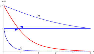
Figure 1: The singular Wu-Yang monopole (the blue line), the two half skyrmions (A) and (B) as partially dressed singular monopoles (blue curves), and the regular skyrmion (red curve) obtained combining the two half skyrmions.

Clearly these solutions carry the unit magnetic charge of the homotopy $\pi_{2}(S^{2})$ defined by $\hat{n}$ ijmpa08

$$M=\dfrac{\pm 1}{8\pi}\int\epsilon_{ijk}\big{[}\hat{r}\cdot(\partial_{i}\hat{r}\times\partial_{j}\hat{r})\big{]}d\sigma_{k}=\pm 1,$$ (43)

but carry a half baryon number

$$B=-\dfrac{1}{8\pi^{2}}\int\epsilon_{ijk}\partial_{i}\omega\big{[}\hat{r}\cdot(\partial_{j}\hat{r}\times\partial_{k}\hat{r})\big{]}\sin^{2}\dfrac{\omega}{2}d^{3}r$$

$$=-\dfrac{1}{\pi}\int\sin^{2}\dfrac{\omega}{2}d\omega=\dfrac{1}{2}.$$ (44)

This is due to the boundary conditions (41) and (42). So it describes a half-skyrmion.

The half-skyrmions have two remarkable features. First, combining the two half-skyrmions we can form a finite energy soliton, the fully dressed skyrmion ijmpa08 . This must be clear because, putting the boundary conditions (41) and (42) together we recover the boundary condition (28) of the skyrmion. So putting the two partially dressed monopoles together we obtain the well known finite energy skyrmion solution.

This is summarized in Fig. 1, where the blue line represents the singular monopole, the dotted curves (A) and (B) represent the singular half skyrmions, and the red curve represents the regular skyrmion. Notice that in all these solutions we have $\hat{n}=\hat{r}$, so that $M=1$. This confirms that the skyrmion is nothing but the Wu-Yang monopole of QCD, transplanted and regularized to have a finite energy by the massless scalar field $\omega$ in the Skyrme theory prl01 ; plb04 ; ijmpa08 .

The other remarkable feature of the half-skyrmions is that the monopole number (43) and the baryon number (44) are different. This is very interesting because, in skyrmions the baryon number is commonly identified by the rational map which defines the monopole number. This suggests that the baryon number and the monopole number are one and the same thing man . But obviously this is not true for the half-skyrmions. In the following we will argue that this need not be ture, and show that the skyrmions in general have two different topological numbers.

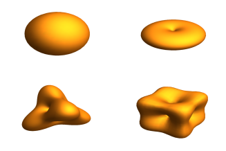
Figure 2: The well known (non spherically symmetric) numerical multi-skyrmion solutions with baryon number 1,2,3,4.

V Skyrmions with Two Topological Numbers

The above argument clearly shows that the skyrmion has the monopole topology. And this monopole topology reappear in all popular non spherically symmetric multi-skyrmion solutions man ; bat ; sut . Indeed, it is well known that the monopole topology of the rational map $\pi_{2}(S^{2})$ given by $\hat{n}$,

$$M=\dfrac{1}{8\pi}\int\epsilon_{ijk}\big{[}\hat{n}\cdot(\partial_{i}\hat{n}\times\partial_{j}\hat{n})\big{]}d\sigma_{k}=m,$$ (45)

together with the boundary condition (28), has played the fundamental role for many people to construct these multi-skyrmion solutions. Some of these multi-skyrmion solutions are shown in Fig. 2.

On the other hand, these solutions have always been interpreted to have the baryon topology $\pi_{3}(S^{3})$ which have the baryon number given by

$$B=-\dfrac{1}{8\pi^{2}}\int\epsilon_{ijk}\partial_{i}\omega\big{[}\hat{n}\cdot(\partial_{j}\hat{n}\times\partial_{k}\hat{n})\big{]}\sin^{2}\dfrac{\omega}{2}d^{3}r$$

$$=\dfrac{1}{8\pi}\int\epsilon_{ijk}\big{[}\hat{n}\cdot(\partial_{i}\hat{n}\times\partial_{j}\hat{n})\big{]}d\sigma_{k}=m.$$ (46)

But obviously this baryon number is precisely the monopole number shown in (45), so that these solutions have $B=M$. Nevertheless, the monopole topology $\pi_{2}(S^{2})$ and the baryon topology $\pi_{3}(S^{3})$ is clearly different. If so, we may ask what is the relation between the monopole topology and the baryon topology.

The Skyrme equation (27) in the spherically symmetric limit plays an important role to clarify this point. To see this notice that, although the SU(2) matrix $U$ is periodic in $\omega$ variable by $4\pi$, $\omega$ itself can take any value from $-\infty$ to $+\infty$. So we can obtain the spherically symmetric multi-skyrmion solutions generalizing the boundary condition (28) to sky ; witt ; prep

$$\omega(0)=2\pi n,~{}~{}~{}~{}~{}\omega(\infty)=0,$$ (47)

with an arbitrary integer $n$. Some of the spherically symmetric multi-skyrmion solutions are shown in Fig. 3. These are, of course, the solutions that Skyrme originally proposed to identify as the nuclei with baryon number larger than one sky . But soon after they are dismissed as uninteresting because they have too much energy.

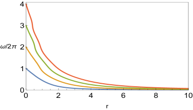
Figure 3: The spherically symmetric skyrmions with baryon number 1,2,3,4, which should be contrasted with the solutions shown in Fig. 2.

An interesting features of the spherically symmetric solutions is that whenever the curve passes through the values $\omega=2\pi n$, it become a bit steeper. This is because (as we will see soon) these points are the vacua of the theory, and the steep slopes shows that the energy likes to be concentrated around these vacua.

Another interesting feature of the spherically symmetric skyrmions is the energy, which is given by ijmpa08

$$E=\dfrac{\pi\kappa^{2}}{2}{\displaystyle\int}_{0}^{\infty}\Big{\{}\Big{(}r^{2}+\dfrac{2\alpha}{\kappa^{2}}\sin^{2}\dfrac{\omega}{2}\Big{)}\Big{(}\dfrac{d\omega}{dr}\Big{)}^{2}$$

$$+8\Big{(}1+\dfrac{\alpha}{2\kappa^{2}r^{2}}\sin^{2}\dfrac{\omega}{2}\Big{)}\sin^{2}\dfrac{\omega}{2}\Big{\}}dr$$

$$=\pi{\sqrt{\alpha}}\kappa{\displaystyle\int}^{\infty}_{0}\Big{[}x^{2}\left(\dfrac{d\omega}{dx}\right)^{2}+8\sin^{2}{\dfrac{\omega}{2}}\Big{]}dx,$$ (48)

where $x=\kappa r/{\sqrt{\alpha}}$. From this we can easily calculate their energy. This is shown in Fig. 4.

Numerically the baryon number dependence of the energy is given by sky ; prep

$$E_{n}\simeq\dfrac{n(n+1)}{2}E_{1}.$$ (49)

This has two remarkable points. First, the baryon number dependence of the energy is quadratic. This, of course, means that the energy of the skyrmion with baryon number $n$ is bigger than the sum of $n$ lowest energy skyrmion. So the radially excited skyrmions are unstable. This is not the case in the popular multi-skyrmion solutions shown in Fig. 2. They have positive binding energy, so that the energy of the skyrmion with baryon number $B$ becomes smaller than the $B$ sum of the lowest energy skyrmion. This was the main reason why the spherically symmetric solutions have not been considered seriously as the model of heavy nuclei.

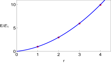
Figure 4: The energy of the spherically symmetric solutions with baryon number 1,2,3,4. The numerical fit (the blue curve) and the $n(n+1)E_{1}/2$ curve (the green curve) are almost indistinguishable.

But actually (49) makes the spherically symmetric solutions mathematically more interesting, because (49) is almost exact. In fact Fig. 4 shows that the mathematical curve $E_{n}=n(n+1)E_{1}/2$ and the numerical fit is almost indistinguishable. We could understand this as follows. Roughly speaking, the kinetic energy (first part) and the potential energy (second part) of (48) become proportional to $n^{2}$ and $n$, and the two terms have an equal contribution due to the equipartition of energy. But we need a better explanation of (49).

Fig. 5 shows the energy density of the solutions. Clearly the $B=n$ solution has $n$ local maxima, which indicates that it is made of n shells of unit skyrmions. Moreover, as we have remarked the energy density has the local maxima at $\omega=2\pi n$. So they describe the shell model of nuclei, made of $n$ shells located at $\omega=2\pi n$. This tells that the spherically symmetric solutions could be viewed as radially extended skyrmions of the original skyrmion. In this interpretation the baryon number $n$ of these skyrmions can be identified as the radial, or more properly the shell, number piet . And this baryon number is fixed by the winding number $\pi_{1}(S^{1})$ of the angular variable $\omega$.

The contrast between the popular non spherically symmetric solutions shown in Fi‍g. 2 and the sphrically symmetric solutions shown in Fig. 3 is unmistakable. But the contrast is not just in the appearance. They are fundamentally different. In particular, the spherically symmetric solutions have a very important implication.

To understand this, notice that these solutions have the monopole number given by

$$M=\dfrac{1}{8\pi}\int\epsilon_{ijk}\big{[}\hat{r}\cdot(\partial_{i}\hat{r}\times\partial_{j}\hat{r})\big{]}d\sigma_{k}=1.$$ (50)

On the other hand, their baryon number is given by the winding number $\pi_{1}(S^{1})$ of $\omega$ determined by the boundary condition (47),

$$B=-\dfrac{1}{8\pi^{2}}\int\epsilon_{ijk}\partial_{i}\omega\big{[}\hat{r}\cdot(\partial_{j}\hat{r}\times\partial_{k}\hat{r})\big{]}\sin^{2}\dfrac{\omega}{2}d^{3}r$$

$$=-\dfrac{1}{\pi}\int\sin^{2}\dfrac{\omega}{2}d\omega=n.$$ (51)

So, unlike the popular non spherically symmetric multi-skyrmions shown in Fig. 2, the baryon number and the monopole number of these solutions are different. Moreover, the baryon number is not given by the rational map, but by the winding number.

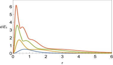
Figure 5: The radial energy density of the spherically symmetric skyrmions with baryon number 1,2,3,4. The density functions are normalized to make the integral of the $B=1$ solution to be the unit.

This confirms that the skyrmions actually do carry two topological numbers, the baryon number of $\pi_{3}(S^{3})$ and the monopole number of $\pi_{2}(S^{2})$ epjc17 . And the spherically symmetric solutions play the crucial role to demonstrate this.

In this scheme the skyrmions are classified by $(m,b)$, the monopole number $m$ and the baryon number $b$. And the popular (non spherically symmetric) solutions become the $(m,m)$ skyrmions and the spherically symmetric solutions become the $(1,n)$ skyrmions.

This has a deep consequence. Based on this we can actually show that the baryon number can be decomposed to the monopole number and the radial (shell) number and expressed by the product of the two numbers epjc17 . To show this we discuss the characteristic features of the spherically symmetric solutions first.

This implies that we could replace the baryon number with the shell number, and classify the skyrmions by the monopole number $m$ and shell number $n$ by $(m,n)$, instead of $(m,b)$. In other words we could also classify the skyrmions by the monopole topology $\pi_{2}(S^{2})$ of $\hat{n}$ and the U(1) (i.e., shell) topology $\pi_{1}(S^{1})$ of $\omega$. In this scheme the baryon number of the $(m,n)$ skyrmion is given by $B=mn$. This must be clear from (29), which tells that the baryon number is made of two parts, the $\pi_{2}(S^{2})$ of $\hat{n}$ and $\pi_{1}(S^{1})$ of $\omega$.

According to this classification the popular (non spherically symmetric) skyrmions become the $(m,1)$ skyrmions, the radially extended spherically symmetric skyrmions become the $(1,n)$ skyrmions. The justification for this classification comes from the following observation. First, the $S^{3}$ space (both the real space and the target space) in the baryon topology $\pi_{3}(S^{3})$ admits the Hopf fibering $S^{3}\simeq S^{2}\times S^{1}$. Second, the two variables $\hat{n}$ and $\omega$ of the Skyrme theory naturally accommodate the monopole topology $\pi_{2}(S^{2})$ and the shell topology $\pi_{1}(S^{1})$.

Furthermore, in this classification the baryon number is given by the product of the monopole number and the shell number, or $B=mn$. To see this notice that the Hopf fibering of $S^{3}$ has an important property that locally it can be viewed as a Cartesian product of $S^{2}$ and $S^{1}$. So we have

$$B=-\dfrac{1}{8\pi^{2}}{\displaystyle\int}\epsilon_{ijk}\partial_{i}\omega\big{[}\hat{n}\cdot(\partial_{j}\hat{n}\times\partial_{k}\hat{n})\big{]}\sin^{2}\dfrac{\omega}{2}d^{3}r$$

$$=-\dfrac{1}{8\pi^{2}}{\displaystyle\int}\partial_{i}\omega\big{[}\hat{n}\cdot(\partial_{j}\hat{n}\times\partial_{k}\hat{n})\big{]}\sin^{2}\dfrac{\omega}{2}dx^{i}\wedge dx^{j}\wedge dx^{k}$$

$$=\dfrac{n}{8\pi}{\displaystyle\int}\epsilon_{ijk}\big{[}\hat{n}\cdot(\partial_{i}\hat{n}\times\partial_{j}\hat{n})\big{]}d\Sigma_{k}=mn,$$ (52)

where $d\Sigma_{k}=\epsilon_{ijk}dx^{i}\wedge dx^{j}/2$. This shows that the baryon number of the skyrmion is given by the product of the monopole number and the shell number. Obviously both $(m,1)$ and $(1,n)$ skyrmions are the particular examples of this.

Another way to show this is to introduce a generalized coordinates $(\eta,\alpha,\beta)$ for $R^{3}$ whose line element is given by

$$ds^{2}=f(\eta)d\eta^{2}+d\Sigma^{2}(\alpha,\beta),$$ (53)

in which $\eta$ represents the radial coordinate $R^{1}$ and $(\alpha,\beta)$ represents the $S^{2}$ such that $\omega=\omega(\eta)$ and $\hat{n}=\hat{n}(\alpha,\beta)$. Again this is possible because the hopf fibering of $S^{3}$ can be expressed by a locally Cartesian product of $S^{2}$ and $S^{1}$. In this coordinates we clearly have

$$B=-\dfrac{1}{8\pi^{2}}{\displaystyle\int}\epsilon_{ijk}\partial_{i}\omega\big{[}\hat{n}\cdot(\partial_{j}\hat{n}\times\partial_{k}\hat{n})\big{]}\sin^{2}\dfrac{\omega}{2}d^{3}x$$

$$=-\dfrac{1}{4\pi^{2}}{\displaystyle\int}\sin^{2}\frac{\omega}{2}d\omega{\displaystyle\int}\big{[}\hat{n}\cdot(d\hat{n}\wedge d\hat{n})\big{]}=mn.$$ (54)

So in this local direct product coordinates, it is straightforward to prove $B=mn$. Notice that the third equality tells that the baryon number can be expressed in a coodinate independent form.

Clearly the spherically symmetric solutions satisfy this criterion. In this case, $\pi_{3}(S^{3})$ naturally decomposes to $\pi_{2}(S^{2})$ of $\hat{n}$ and $\pi_{1}(S^{1})$ of $\omega$, so that the baryon number $B$ is decomposed to the $S^{2}$ wrapping number $m$ and the $S^{1}$ winding number $n$. But the spherical symmetry requires $\hat{n}=\hat{r}$, and restricts $m=1$.

Again this follows from two facts. First, the fact that the Hopf fibering allows $S^{3}$ to decompose $S^{2}\times S^{1}$, and the fact that in Skurme theory $\omega$ and $\hat{n}$ naturally decompose the target space $S^{3}$ to $S^{1}$ and $S^{2}$. With this we have $\pi_{3}(S^{3})\simeq\pi_{2}(S^{2})\times\pi_{1}(S^{1})$. This strongly support that the baryon topology $\pi_{3}(S^{3})$ can be refined to $\pi_{2}(S^{2})$ of $\hat{n}$ and $\pi_{1}(S^{1})$ of $\omega$.

If so, one might wonder whether the popular skyrmions can also be made to carry two different topological numbers. This should be possible. To see this remember that the integer $n$ in the $(1,n)$ skyrmions describes the radial (shell) number which describes the shell structure of the spherically symmetric skyrmions. And this shell structure is provided by the angular variable $\omega$ which allows the radial extension of the original $(1,1)$ skyrmion. So we can generalize the $(m,1)$ skyrmion to have similar shell structure.

In fact, we may obtain the “radially extended” solutions of the non spherically symmetric skyrmions numerically, generalizing the boundary condition (28) to (47), requiring piet

$$\omega(r_{k})=2\pi k,~{}~{}~{}(k=0,1,2,...n),$$

$$r_{0}=0~{}\langle~{}r_{1}~{}\langle~{}...~{}\langle~{}r_{n}=\infty,$$ (55)

keeping the rational map number $m$ of $\hat{n}$ unchanged. With this we could find new solutions numerically minimizing the energy, varying $r_{k}~{}(k=1,2,...,n-1)$. This way we can add the shell structure and the shell number to the $(m,m)$ skyrmion. In this case the baryon number of the radially extended skyrmions should become $B=mn$.

But the above argument tells that in general (even for non spherically symmetric skyrmions) we may introduce the generalized coordinates such that $\hat{n}=\hat{n}(\alpha,\beta)$ and $\omega=\omega(\gamma)$, and can still make the “radial” extension of the skyrmions to obtain the radially extended $(m,n)$ skyrmions which have $n$ shells numerically, generalizing the boundary condition (28) to (47).

Again this becomes possible because the Skyrme theory is described by two variables $\hat{n}$ and $\omega$ which naturally accommodate the monopole topology $\pi_{2}(S^{2})$ and the shell topology $\pi_{1}(S^{1})$. This is very important, because mathematically there is no way to justify the replacement of the $\pi_{3}(S^{3})$ topology by two independent $\pi_{2}(S^{2})$ topology and $\pi_{1}(S^{1})$ topology.

Now, one may ask about the stability of the $(m,n)$ skyrmions. Clearly an $(m,n)$ skyrmion does not have to be stable, and could decay to lower energy skyrmions as far as the decay is energetically allowed. For example, (49) clearly tells that the $(1,n)$ skyrmion can decay to lower energy skyrmions. This is natural. An interesting and important question here is whether the two topological numbers $m$ and $n$ are conserved independently or not. Certainly the baryon topology and the monopole topology are mathematically independent. This means that the baryon number and the monopole number must be conserved separately. This (with $\delta B=m~{}\delta n+n~{}\delta m$) automatically guarantees that the shell number must also be conserved.

This means that the two numbers $m$ and $n$ must be conserved separately, so that the $(n,m)$ skyrmion could decay to $(n_{1},m_{1})$ and $(n_{2},m_{2})$ skyrmions when $n=n_{1}+n_{2}$ and $m=m_{1}+m_{2}$. But there is no way that the two topological numbers $m$ and $n$ can be transformed to each other. This tells that the skyrmions retains the topological stability of two topology independently, even when they are classified by two topologial numbers.

The above discussions raise another deep question. As we have remarked, when $\omega=(2n+1)\pi$, the Skyrme theory reduces to the Skyrme-Faddeev theory. In this limit the Skyrme theory has the knot solutions described by $\hat{n}$ whose topology is given by $\pi_{3}(S^{2})$ prl01 ; plb04 ; ijmpa08 . And in these knots, $\omega$ is not activated. If so, one might ask if we can dress the knots with $\omega$ and add the shell structure to the knots to have two topological numbers $\pi_{1}(S^{1})$ and $\pi_{3}(S^{2})$. This is a mind boggling question which certainly deserves more study.

VI Multiple Vacua of Skyrme Theory

Skyrme theory has been known to have rich topological structures. It has the Wu-Yang type monopoles which have the $\pi_{2}(S^{2})$ topology, the skyrmions which have the $\pi_{3}(S^{3})$ topology, the baby skyrmions which have the $\pi_{1}(S^{1})$ topology, and the Faddeev-Niemi knots which have the $\pi_{3}(S^{2})$ topology prl01 ; plb04 ; ijmpa08 . In the above we have shown that the theory has more topological structure, and proved that the skyrmions can be generalized to have two topological quantum numbers. But this is not the end of story.

The Skyrme theory in fact has another very important topological structure, the topologically different multiple vacua. To see this, notice that (23) has the solution

$$\omega=2\pi p,~{}~{}~{}(p;~{}integer),$$ (56)

independent of $\hat{n}$. Clearly this is the vacuum solution.

This shows that the Skyrme theory has multiple vacua classified by the integer $p$. This is similar to the vacuum of the Sine-Gordon theory, but we emphasize that, unlike the Sine-Gordon theory, the Skyrme theory has the multiple vacua without any potential. Of course, we could have such vacua in Skyrme theory introducing a potential term in the Lagrangian. This is not what we are doing here. Another pont is that the spherically symmetric skyrmions occupy and connect the $p+1$ adjacent vacua. This tells that we can connect all vacua with the spherically symmetric skyrmions.

Perhaps more importantly, (56) becomes the vacuum independent of $\hat{n}$, which is completely arbitrary. So $\hat{n}$ can add the $\pi_{3}(S^{2})$ topology to each of the multiple vacua classified by another integer $q$. And this topology is precisely the knot topology of the QCD vacuum plb07 .

This is not surprising. In view of the deep connection between QCD and Skyrme theory, it is natural that they have similar vacuum structure. To clarify this point we introduce a right-handed unit isotriplet $(\hat{n}_{1},\hat{n}_{2},\hat{n}_{3}=\hat{n})$, and impose the vacuum isometry to the SU(2) gauge potential,

$${}^{\forall_{i}}D_{\mu}\hat{n}_{i}=0,$$ (57)

which assures $\vec{F}_{\mu\nu}=0$. From this we obtain the most general SU(2) QCD vacuum potential plb07

$${\vec{A}}_{\mu}\rightarrow\hat{\Omega}_{\mu}=-\dfrac{1}{2}\epsilon_{ijk}(\hat{n}_{i}\cdot\partial_{\mu}\hat{n}_{j})~{}\hat{n}_{k}$$

$$=\dfrac{1}{2}\epsilon_{ijk}(\hat{n}_{i}\cdot\partial_{\mu}\hat{n}_{j})~{}\hat{e}_{k},$$ (58)

where $\hat{e}_{1}=(1,0,0),\hat{e}_{2}=(0,1,0),\hat{e}_{3}=(0,0,1)$.

This is the QCD vacuum which has the knot topology $\pi_{3}(S^{3})\simeq\pi_{3}(S^{2})$. It is clear that (58) describes the $\pi_{3}(S^{3})$ topology, since $(\hat{n}_{1},\hat{n}_{2},\hat{n})$ defines the mapping $\pi_{3}(S^{3})$ from the compactified 3-dimensional space to the SU(2) group space. But notice that $(\hat{n}_{1},\hat{n}_{2},\hat{n})$ is completely determined by $\hat{n}$, up to the U(1) rotation which leaves $\hat{n}$ invariant, which describes the mapping from the real space $S^{3}$ to the coset space $S^{2}$ of $SU(2)/U(1)$. So the QCD vacuum (58) can also be classified by the knot topology $\pi_{3}(S^{2})$ plb07 .

Now it becomes clear why the Skyrme theory has the same knot topology. As we have noticed, the Skyrme theory has the vacuum (56), independent of $\hat{n}$. But this $\hat{n}$ (just as in the SU(2) QCD) defines the mapping $\pi_{3}(S^{2})$, with the $S^{3}$ compactification of $R^{3}$, and thus can be classified by the knot topology. Of course, in the Skyrme theory we do not need the vacuum potential (58) to describe the vacuum. All we need to describe the knot topology is $\hat{n}$.

This tells that the vacuum of the Skyrme theory has the topology of the Sine-Gordon theory and QCD combined together. So the vacuum of the Skyrme theory can also be classified by two topologcal numbers $(p,q)$, the $\pi_{1}(S^{1})$ of $\omega$ and $\pi_{3}(S^{2})$ of $\hat{n}$. And this is so without any extra potential. As we know, there is no other theory which has this type of vacuum topology.

The multiple vacua leads us to the question if the Skyrme theory has a vacuum tunneling which connects these vacua. Certainly this is a very interesting question worth to be studied further.

Before we close we emphasize the followings. First, the knot topology $\pi_{3}(S^{2})$ of $\hat{n}$ of the vacuum is different from the monopole topology $\pi_{2}(S^{2})$ of $\hat{n}$. The monopole topology is associated to the isolated singularities of $\hat{n}$, but for the knot topology $\hat{n}$ does not have any singularity for. For the vacuum $\hat{n}$ must be completely regular everywhere.

Second, the knot topology of the vacuum is different from the Faddeev-Niemi knot in the Skyrme theory prl01 . The Faddeev-Niemi knot is a real knot which carries energy, but the vacuum knot has no energy. Moreover, we have the knot solution when $\omega=(2n+1)\pi$, but we have the knot of the vacuum when $\omega=2\pi p$. In addition, there are infinitely many $\hat{n}$ which describes the same vacuum knot topology, while the Faddeev-Niemi knot is unique.

What is really remarkable here is that the same $\hat{n}$ has multiple roles. It describes the monopole topology of the skyrmion, the knot topology of Faddeev-Niemi knot, and the knot topology of the vacuum.

VII Knot in Skyrme Theory

It is well known that in Skyrme theory has the baby skyrmions, the magnetic vortex made of monopole-antimonopole pair infinitely separated apart piet . Moreover, with this we can construct the helical baby skyrmion, twisting the magnetic vortex ijmpa08 . But the helical vortex becomes unstable and decays to the untwisted baby skyrmion, unless the periodicity condition is enforced by hand. A natural way to make the helical baby skyrmion stable is to make it a knot connecting two periodic ends and making it a twisted magnetic vortex ring.

By construction this twisted vortex ring carries two magnetic fluxes, $m$ unit of flux passing through the disk of the ring and $n$ unit of flux moving along the ring. Moreover the two fluxes can be thought of two closed rings linked together winding each other $m$ and $n$ times, whose linking number becomes $mn$. This tells that the twisted vortex ring becomes a knot prl01 ; plb04 ; ijmpa08 .

To confirm this we solve the knot equation (25) explicitly with a consistent ansatz. We first adopt the toroidal coordinates $(\eta,\gamma,\varphi)$ given by

$$x=\dfrac{a}{D}\sinh{\eta}\cos{\varphi},~{}~{}~{}y=\dfrac{a}{D}\sinh{\eta}\sin{\varphi},$$

$$z=\dfrac{a}{D}\sin{\gamma},~{}~{}~{}D=\cosh{\eta}-\cos{\gamma},$$

$$ds^{2}=\dfrac{a^{2}}{D^{2}}\Big{(}d\eta^{2}+d\gamma^{2}+\sinh^{2}\eta d\varphi^{2}\Big{)},$$

$$d^{3}x=\dfrac{a^{3}}{D^{3}}\sinh{\eta}d\eta d\gamma d\varphi,$$ (59)

where $a$ is the radius of the knot defined by $\eta=\infty$. With this we choose the following axially symmetric ansatz

$$\hat{n}=\left(\begin{array}[]{cc}\sin f\cos(n\beta+m\varphi)\\ \sin f\sin(n\beta+m\varphi)\cr\cos f\end{array}\right),$$ (63)

where $f$ and $\beta$ are functions of $\eta$ and $\gamma$.

With this we have

$$C_{\mu}=n(\cos f-1)\partial_{\mu}\beta+m(\cos f+1)\partial_{\mu}\varphi,$$

$$H_{\eta\gamma}=-nK\sin f,~{}~{}~{}~{}H_{\gamma\varphi}=-m\sin f\partial_{\gamma}f,$$

$$H_{\varphi\eta}=m\sin f\partial_{\eta}f,$$

$$K=\partial_{\eta}f\partial_{\gamma}\beta-\partial_{\gamma}f\partial_{\eta}\beta,$$ (64)

so that the knot equation (25) is written as

$$\Big{[}\partial_{\eta}^{2}+\partial_{\gamma}^{2}+\Big{(}\dfrac{\cosh\eta}{\sinh\eta}-\dfrac{\sinh\eta}{D}\Big{)}\partial_{\eta}-\dfrac{\sin\gamma}{D}\partial_{\gamma}\Big{]}f$$

$$-\Big{(}n^{2}\big{(}(\partial_{\eta}\omega)^{2}+(\partial_{\gamma}\omega)^{2}\big{)}+\dfrac{m^{2}}{\sinh^{2}\eta}\Big{)}\sin f\cos f$$

$$+\dfrac{\alpha}{\kappa^{2}}\dfrac{D^{2}}{a^{2}}\Big{(}A\cos f+B\sin f\Big{)}\sin f=0,$$

$$\Big{[}\partial_{\eta}^{2}+\partial_{\gamma}^{2}+\Big{(}\dfrac{\cosh\eta}{\sinh\eta}-\dfrac{\sinh\eta}{D}\Big{)}\partial_{\eta}-\dfrac{\sin\gamma}{D}\partial_{\gamma}\Big{]}\beta$$

$$+2\Big{(}\partial_{\eta}f\partial_{\eta}\beta+\partial_{\gamma}f\partial_{\gamma}\beta\Big{)}\dfrac{\cos f}{\sin f}$$

$$-\dfrac{\alpha}{\kappa^{2}}\dfrac{D^{2}}{a^{2}}C=0,$$ (65)

where

$$A=\Big{[}n^{2}K^{2}+\dfrac{m^{2}}{\sinh^{2}\eta}\Big{(}(\partial_{\eta}f)^{2}+(\partial_{\gamma}f)^{2}\Big{)}\Big{]},$$

$$B=\Big{\{}n^{2}\partial_{\eta}K\partial_{\gamma}\beta-n^{2}\partial_{\gamma}K\partial_{\eta}\beta$$

$$+n^{2}K\Big{[}\Big{(}\dfrac{\cosh\eta}{\sinh\eta}+\dfrac{\sinh\eta}{D}\Big{)}\partial_{\gamma}\beta-\dfrac{\sin\gamma}{D}\partial_{\eta}\beta\Big{]}$$

$$+\dfrac{m^{2}}{\sinh^{2}\eta}\Big{[}\partial_{\eta}^{2}+\partial_{\gamma}^{2}-\Big{(}\dfrac{\cosh\eta}{\sinh\eta}-\dfrac{\sinh\eta}{D}\Big{)}\partial_{\eta}+\dfrac{\sin\gamma}{D}\partial_{\gamma}\Big{]}f\Big{\}},$$

$$C=\Big{\{}\partial_{\eta}K\partial_{\gamma}f-\partial_{\eta}f\partial_{\gamma}K$$

$$+K\Big{[}\Big{(}\dfrac{\cosh\eta}{\sinh\eta}+\dfrac{\sinh\eta}{D}\Big{)}\partial_{\gamma}-\dfrac{\sin\gamma}{D}\partial_{\eta}\Big{)}f\Big{\}}.$$

With the ansatz (63) the knot energy is given by

$$E={\sqrt{\alpha}}\kappa{\displaystyle\int}\Big{\{}\dfrac{\kappa}{\sqrt{\alpha}}\dfrac{a}{2D}\Big{[}(\partial_{\eta}f)^{2}+(\partial_{\gamma}f)^{2}$$

$$+\Big{(}n^{2}\big{(}(\partial_{\eta}\beta)^{2}+(\partial_{\gamma}\beta)^{2}\big{)}+\dfrac{m^{2}}{\sinh^{2}\eta}\Big{)}\sin^{2}f\Big{]}$$

$$+\dfrac{\sqrt{\alpha}}{\kappa}\dfrac{D}{4a}\Big{[}n^{2}K^{2}+\dfrac{m^{2}}{\sinh^{2}\eta}\Big{(}(\partial_{\eta}f)^{2}$$

$$+(\partial_{\gamma}f)^{2}\Big{)}\Big{]}\sin^{2}f\Big{\}}\sinh\eta d\eta d\gamma d\varphi.$$ (66)

Minimizing the energy we reproduce the knot equation (65), which confirms that ansatz (63) is consistent.

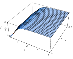
Figure 6: (Color online). The $f$ configuration of the knot with $m=n=1$ in Skyrme theory. Notice that here $\eta$ is dimensionless.

In toroidal coordinates, $\eta=\gamma=0$ represents spatial infinity and $\eta=\infty$ describes the torus center. So we can try to obtain the knot solution imposing the following boundary condition

$$f(0,\gamma)=0,~{}~{}~{}~{}~{}f(\infty,\gamma)=\pi,$$

$$\beta(\eta,0)=0,~{}~{}~{}~{}~{}\beta(\eta,2\pi)=2\pi.$$ (67)

Of course, an exact solution of (65) is extremely difficult to obtain, even numerically. In fact many known “knot solutions” are actually the energy profile of knots which minimizes the Hamiltonian fadd . But here with the ansatz (63) we can find an actual profile of the knot. For $m=n=1$ the knot radius $a$ which minimizes the energy is given by

$$a\simeq 1.21~{}\dfrac{\sqrt{\alpha}}{\kappa}.$$ (68)

From this we obtain Fig. 6 and Fig. 7 which shows the knot profile for $f$ and $\omega$ of the lightest axially symmetric knot solution.

With the numerical solution we can check the topology of the knot. From the ansatz (63) we have the knot number

$$Q_{k}=\dfrac{1}{32\pi^{2}}{\displaystyle\int}\epsilon_{ijk}~{}C_{i}~{}H_{jk}d^{3}x$$

$$=\dfrac{mn}{8\pi^{2}}{\displaystyle\int}K\sin fd\eta d\gamma d\varphi=\dfrac{mn}{4\pi}{\displaystyle\int}\sin fdfd\beta$$

$$=mn,$$ (69)

where the last equality comes from the boundary condition (67). This assures that our ansatz describes the correct knot topology. Notice this is formally identical to the Chern-Simon integral of the helicity of the electromagnetic knot shown in (2).

To clarify the meaning of (69) we now calculate the magnetic flux of the knot. The helical magnetic field has two magnetic fluxes, $\Phi_{\hat{\gamma}}$ passing through the knot disk of radius $a$ in the $xy$-plane and $\Phi_{\hat{\varphi}}$ moving along the knot ring of radius $a$, given by

$$\Phi_{\hat{\gamma}}={\displaystyle\int}_{\gamma=\pi}H_{\hat{\gamma}}\dfrac{a^{2}\sinh\eta}{D^{2}}d\eta d\varphi$$

$$=m{\displaystyle\int}_{\gamma=\pi}\sin f\partial_{\eta}fd\eta d\varphi=4\pi m,$$

$$\Phi_{\hat{\varphi}}={\displaystyle\int}H_{\hat{\varphi}}\dfrac{a^{2}}{D^{2}}d\eta d\gamma=n{\displaystyle\int}K\sin fd\eta d\gamma$$

$$=4\pi n.$$ (70)

This confirms the followings. First, the flux is quantized in the unit of $4\pi$. Second, the two fluxes are linked, whose linking number is given by $mn$. This is precisely the knot number (69). This provides the physical interpretation of the topological knot.

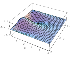
Figure 7: (Color online). The $\beta$ configuration of the knot with $m=n=1$ in Skyrme theory. Notice that here the actual configuration shown is $\beta-\gamma$.

The supercurrent which generates the twisted magnetic flux of the knot is given by the conserved current density

$$j_{\mu}=\dfrac{nD^{2}}{a^{2}}\Big{(}\partial_{\eta}+\dfrac{\cosh\eta}{\sinh\eta}+\dfrac{\sinh\eta}{D}\Big{)}K\partial_{\mu}\gamma$$

$$+\dfrac{mD^{2}}{a^{2}}\Big{[}\Big{(}\partial_{\eta}-\dfrac{\cosh\eta}{\sinh\eta}+\dfrac{\sinh\eta}{D}\Big{)}\sin f\partial_{\eta}f$$

$$+\Big{(}\partial_{\gamma}+\dfrac{\sin\gamma}{D}\Big{)}\sin f\partial_{\gamma}f\Big{]}\partial_{\mu}\varphi.$$ (71)

From this we have two quantized supercurrents, $i_{\hat{\gamma}}$ which flows through the knot disk and $i_{\hat{\varphi}}$ which flows along the knot,

$$i_{\hat{\gamma}}={\displaystyle\int}_{\gamma=\pi}j_{\hat{\gamma}}(\eta,\gamma)\dfrac{a^{2}\sinh\eta}{D^{2}}d\eta d\varphi$$

$$=\dfrac{n}{a}{\displaystyle\int}_{\gamma=\pi}D\sinh\eta\Big{(}\partial_{\eta}+\dfrac{\cosh\eta}{\sinh\eta}+\dfrac{\sinh\eta}{D}\Big{)}Kd\eta d\varphi,$$

$$i_{\hat{\varphi}}={\displaystyle\int}j_{\hat{\varphi}}\dfrac{a^{2}}{D^{2}}d\eta d\gamma$$

$$=\dfrac{m}{a}{\displaystyle\int}\dfrac{D}{\sinh\eta}\Big{[}\Big{(}\partial_{\eta}-\dfrac{\cosh\eta}{\sinh\eta}+\dfrac{\sinh\eta}{D}\Big{)}\sin f\partial_{\eta}f$$

$$+\Big{(}\partial_{\gamma}+\dfrac{\sin\gamma}{D}\Big{)}\sin f\partial_{\gamma}f\Big{]}d\eta d\gamma.$$ (72)

For $m=n=1$ we find numerically

$$i_{\hat{\gamma}}\simeq\dfrac{23.9}{a},~{}~{}~{}~{}~{}i_{\hat{\varphi}}\simeq 0.$$ (73)

Notice that $i_{\hat{\varphi}}$ is vanishing, but the current density $j_{\hat{\varphi}}$ is non-trivial. This tells that the knot has a net angular momentum around the symmetric axis which stablizes the knot.

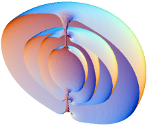
Figure 8: (Color online). The 3-dimensional energy profile of the lightest axially symmetric knot with $m=n=1$ in Skyrme theory. Here the scale is in the unit of ${\sqrt{\alpha}}/\kappa$.

One might wonder how big is the knot. The numerical result suggests that the radius of the vortex (the thickness of the knot) $r_{0}$ is roughly given by

$$r_{0}\simeq a~{}{\rm csch}~{}2\simeq\dfrac{1}{3}\dfrac{\sqrt{\alpha}}{\kappa}.$$ (74)

This shows that the radius of the vortex ring is about 3.6 times the radius of the vortex. From this we can construct a 3-dimensional energy profile of the knot. This is shown in Fig. 8.

In mathematics the knot is described by the linking number of the preimage of the Hopf mapping. When the preimages of two points of the target space are linked, the mapping defines a knot. And the knot number of $\pi_{3}(S^{2})$ is given by the linking number of two preimages fixed by the Chern-Simon index (69) of the potential $C_{\mu}$.

The above result provides an alternative picture of knot. It shows that two real (physical) magnetic flux rings linked together makes the knot, whose knot number is given by the linking number of two flux rings. Clearly this is different from the above mathematical definition of knot based on the Hopf mapping. This is a dynamical manifestation of knot, the linking of two physical flux rings generated by dynamics plb04 .

Obviously two flux rings linked together can not be unlinked by any smooth deformation of the flux ring. This guarantees the topological stability of the knot. Moreover, this topological stability is backed up by the dynamical stability which comes from the dynamics of the flux ring. This is because the supercurrent which generates the quantized magnetic flux of the knot has two components, the one moving along the knot, and the other moving around the knot tube. And the supercurrent moving along the knot generates non-vanishing angular momentum around the $z$-axis, which provides the centrifugal force preventing the vortex ring to collapse. This is how the knot acquires the dynamical stability plb04 .

As we have argued, the knot is stable within the framework of Skyrme-Faddeev theory. However, we have to be cautious about the knot stability in Skyrme theory. This is because the Skyrme theory has the extra massless scalar field $\omega$ which (in principle) could destabilize the knot. So in Skyrme theory the proof of the stability of the knot becomes a non-trivial matter.

VIII Knots in Condensed Matter Physics

The knots can also appear in two-component superfluid and two-gap superconductor pra05 ; prb06 ; epjb08 . To see this let $\phi$ be a complex doublet which describes a two-component Bose-Einstein condensate (BEC)

$$\phi=\dfrac{1}{\sqrt{2}}\rho~{}\xi,~{}~{}~{}~{}~{}(\xi^{\dagger}\xi=1)$$ (75)

and consider the following “gauged” Gross-Pitaevskii type Lagrangian pra05

$${\cal L}=-|D_{\mu}\phi|^{2}-\dfrac{\lambda}{2}\big{(}\phi^{\dagger}\phi-\dfrac{\kappa^{2}}{\lambda}\big{)}^{2}-\dfrac{1}{4}F_{\mu\nu}^{2},$$ (76)

where $D_{\mu}=\partial_{\mu}+igA_{\mu}$, $\kappa^{2}$ and $\lambda$ are the coupling constants. Of course, since we are interested in a neutral condensate, we identify the potential $A_{\mu}$ with the velocity field of $\xi$

$$gA_{\mu}=-i\xi^{\dagger}\partial_{\mu}\xi.$$ (77)

With this the Lagrangian (76) is reduced to

$${\cal L}=-\dfrac{1}{2}(\partial_{\mu}\rho)^{2}-\dfrac{\rho^{2}}{2}\Big{(}|\partial_{\mu}\xi|^{2}-|\xi^{\dagger}\partial_{\mu}\xi|^{2}\Big{)}$$

$$-\dfrac{\lambda}{8}\Big{(}\rho^{2}-\rho_{0}^{2}\Big{)}^{2}+\dfrac{1}{4g^{2}}(\partial_{\mu}\xi^{\dagger}\partial_{\nu}\xi-\partial_{\nu}\xi^{\dagger}\partial_{\mu}\xi)^{2},$$

$$\rho_{0}^{2}=\dfrac{2\kappa^{2}}{\lambda}.$$ (78)

Notice that here the gauge field strength $F_{\mu\nu}$ is replaced by the non-vanishing vorticity of the velocity field (77), but the Lagrangian still retains the $U(1)$ gauge symmetry of (76).

From the Lagrangian we have the following equation of motion

$$\partial^{2}\rho-\Big{(}|\partial_{\mu}\xi|^{2}-|\xi^{\dagger}\partial_{\mu}\xi|^{2}\Big{)}\rho=\dfrac{\lambda}{2}(\rho^{2}-\rho_{0}^{2})\rho,$$

$$\Big{\{}(\partial^{2}-\xi^{\dagger}\partial^{2}\xi)+2\Big{(}\dfrac{\partial_{\mu}\rho}{\rho}-\xi^{\dagger}\partial_{\mu}\xi$$

$$+\dfrac{1}{g^{2}\rho^{2}}\partial_{\alpha}(\partial_{\mu}\xi^{\dagger}\partial_{\alpha}\xi-\partial_{\alpha}\xi^{\dagger}\partial_{\mu}\xi)\Big{)}(\partial_{\mu}-\xi^{\dagger}\partial_{\mu}\xi)\Big{\}}\xi$$

$$=0.$$ (79)

But remarkably, with

$$\hat{n}=\xi^{\dagger}\vec{\sigma}\xi,$$ (80)

we have

$$(\partial_{\mu}\hat{n})^{2}=4(|\partial_{\mu}\xi|^{2}-|\xi^{\dagger}\partial_{\mu}\xi|^{2})$$

$$H_{\mu\nu}=\hat{n}\cdot(\partial_{\mu}\hat{n}\times\partial_{\nu}\hat{n})=-2i(\partial_{\mu}\xi^{\dagger}\partial_{\nu}\xi-\partial_{\nu}\xi^{\dagger}\partial_{\mu}\xi)$$

$$=\partial_{\mu}C_{\nu}-\partial_{\nu}C_{\mu}.$$ (81)

This tells that the velocity potential (77) plays the role of the magnetic potential $C_{\mu}$ in (25) of Skyrme theory.

With (81) the Lagrangian (78) is reduced to the following $CP^{1}$ Lagrangian

$${\cal L}=-\dfrac{1}{2}(\partial_{\mu}\rho)^{2}-\dfrac{\rho^{2}}{2}(\partial_{\mu}\hat{n})^{2}-\dfrac{\lambda}{8}(\rho^{2}-\rho_{0}^{2})^{2}$$

$$-\dfrac{1}{16g^{2}}(\partial_{\mu}\hat{n}\times\partial_{\nu}\hat{n})^{2}.$$ (82)

Furthermore the equation (79) can be put into the form

$$\partial^{2}\rho-\dfrac{1}{4}(\partial_{i}\hat{n})^{2}\rho=\dfrac{\lambda}{2}(\rho^{2}-\rho_{0}^{2})\rho,$$

$$\hat{n}\times\partial^{2}\hat{n}+2\dfrac{\partial_{i}\rho}{\rho}\hat{n}\times\partial_{i}\hat{n}+\dfrac{1}{g^{2}\rho^{2}}\partial_{i}H_{ij}\partial_{j}\hat{n}=0.$$ (83)

The reason why we can express (79) completely in terms of $\hat{n}$ (and $\rho$) is that the Abelian gauge invariance of (76) effectively reduces the target space of $\xi$ to the gauge orbit space $S^{2}=S^{3}/S^{1}$, which is identical to the target space of $\hat{n}$.

This analysis clearly shows that the above theory of two-component BEC is closely related to the Skyrme theory. In fact, in the vacuum $\rho^{2}=\rho_{0}^{2}$ the Lagrangian reduces to the Skyrme-Faddeev Lagrangian

$${\cal L}=-\dfrac{\rho_{0}^{2}}{2}\Big{(}|\partial_{\mu}\xi|^{2}-|\xi^{\dagger}\partial_{\mu}\xi|^{2}\Big{)}$$

$$-\dfrac{1}{4g^{2}}(\partial_{\mu}\xi^{\dagger}\partial_{\nu}\xi-\partial_{\nu}\xi^{\dagger}\partial_{\mu}\xi)^{2}$$

$$=-\dfrac{\rho_{0}^{2}}{2}(\partial_{\mu}\hat{n})^{2}-\dfrac{1}{16g^{2}}(\partial_{\mu}\hat{n}\times\partial_{\nu}\hat{n})^{2}.$$ (84)

This shows that the three Lagrangians (30), (40), and (84) are all identical to each other, which confirms that the Skyrme theory and the theory of two-component superfluid are indeed very similar. This implies that the Skyrme-Faddeev theory could also be regarded as a theory of two-component superfluid.

Figure 9: The non-Abelian vortex (dashed line) with $m=0,n=1$ and the helical vortex (solid line) with $m=n=1$ in the gauge theory of two-component BEC. Here we have put $\lambda/g^{2}=1$, $k=0.64~{}{\sqrt{\lambda}}\rho_{0}$, and $\varrho$ is in the unit of $1/{\sqrt{\lambda}}\rho_{0}$.

The above observation also reveals two important facts. First, it tells that the Skyrme theory has a $U(1)$ gauge symmetry as we have demonstrated in (22). Indeed, it is this gauge symmetry which allows us to establish the existence of the Meissner effect in Skyrme theory. Second, it provides a new meaning to $H_{\mu\nu}$. The two-form now describes the vorticity of the velocity field of the superfluid $\xi$. In other words, the non-linear Skyrme interaction can be interpreted as the vorticity interaction of the superfluid. It is well-known that the vorticity plays an important role in superfluid ho . But creating a vorticity in superfluid costs energy. So it makes a perfect sense to include the vorticity interaction in the theory of superfluid. And the Skyrme-Faddeev Lagrangian naturally contains this interaction.

Moreover, the above observation makes it clear that the above gauge theory of two-component BEC has a knot very similar to the Faddeev-Niemi knot pra05 ; prb06 . Indeed with the following knot ansatz for two-component BEC

$$\phi=\dfrac{1}{\sqrt{2}}\rho(\eta,\gamma)\xi,$$

$$\xi=\left(\begin{array}[]{cc}\cos\dfrac{f(\eta,\gamma)}{2}\exp(-im\varphi)\\ \sin\dfrac{f(\eta,\gamma)}{2}\exp(in\beta(\eta,\gamma))\end{array}\right),$$ (87)

we have

$$\hat{n}=\xi^{\dagger}\vec{\sigma}\xi=\left(\begin{array}[]{ccc}sinf\cos(n\beta+m\varphi)\\ \sin f\sin(n\beta+m\varphi)\\ \cos f\end{array}\right),$$ (91)

$$C_{\mu}=-2i\xi^{\dagger}\partial_{\mu}\xi$$

$$=n(\cos f-1)\partial_{\mu}\beta+m(\cos f+1)\partial_{\mu}\varphi.$$

Clearly this is identical to the Faddeev-Niemi knot ansatz shown in (63). With the ansatz (87) we can obtain a knot solution very similar to the Faddeev-Niemi knot pra05 ; prb06 . This is shown in Fig. 9. The only difference between the two knots is that the one in BEC has a dressing of an extra scalar field $\rho$ which represents the degree of the condensation.

Clearly the knot in two component BEC describes a vorticity knot. And here the complex doublet $\xi$ provides the knot topology,

$$Q_{k}=\dfrac{1}{4\pi^{2}}{\displaystyle\int}\epsilon_{ijk}\xi^{\dagger}\partial_{i}\xi(\partial_{j}\xi^{\dagger}\partial_{k}\xi)d^{3}x$$

$$=\dfrac{1}{32\pi^{2}}{\displaystyle\int}\epsilon_{ijk}C_{i}H_{jk}d^{3}x.$$ (92)

This is the Chern-Simon index which is mathematically identical to the helicity (2) of the electromagnetic knot.

But $\xi$ defines the mapping $\pi_{3}(S^{3})$ from the compactified space $S^{3}$ to the target space $S^{3}$. Apparently this is the baryon topology of the skyrmion, not the knot topology $\pi_{3}(S^{2})$. This has led to a misleading statement in the literature that the vorticity knot can be identified as a skyrmion batt . But this is wrong. The reason is that the target space has the Hopf fibering $S^{3}\simeq S^{2}\times S^{1}$, and the hidden $U(1)$ gauge symmetry in BEC effectively reduces the target space to $S^{2}$, so that $\pi_{3}(S^{3})$ defined by $\xi$ actually reduces to $\pi_{3}(S^{2})$. So actually the knot topology here is described by $\hat{n}$ given by (VIII). In comparoson in Skyrme theory the scalar field $\omega$ describes the $S^{1}$ fiber, so that the baryon topology $\pi_{3}(S^{3})$ can not be reduced to $\pi_{3}(S^{2})$.

We can have similar knot in multi-gap superconductors prb06 ; epjb08 . In the above BEC the gauge interaction was a self-induced interaction. But when the doublet is charged, the gauge interaction can be treated as independent. In this case the theory can describe a two-gap superconductor. But even in this case the knot topology and thus the knot itself should survive. This implies that two-gap superconductor could also have a topological knot.

The knot in two-gap superconductor could be either relativistic or non-relativistic, and appear in both Abelian and non-Abelian setting pra05 ; prb06 . In this paper we will discuss the relativistic knot in the Abelian setting (a non-relativistic Gross-Pitaevskii type theory gives an identical result). Consider a charged doublet scalar field $\phi$ coupled to real electromagnetic field,

$${\cal L}=-|D_{\mu}\phi|^{2}+\kappa^{2}\phi^{\dagger}\phi-\dfrac{\lambda}{2}(\phi^{\dagger}\phi)^{2}-\dfrac{1}{4}F_{\mu\nu}^{2},$$

$$D_{\mu}\phi=(\partial_{\mu}-igA_{\mu})\phi.$$ (93)

The Lagrangian has the equation of motion

$$D^{2}\phi=\lambda(\phi^{\dagger}\phi-\dfrac{\kappa^{2}}{\lambda})\phi,$$

$$\partial_{\mu}F_{\mu\nu}=j_{\nu}=ig\Big{[}(D_{\nu}\phi)^{\dagger}\phi-\phi^{\dagger}(D_{\nu}\phi)\Big{]}.$$ (94)

Now, with

$$\phi=\dfrac{1}{\sqrt{2}}\rho\xi,~{}~{}~{}~{}~{}{\xi}^{\dagger}\xi=1,~{}~{}~{}~{}~{}\hat{n}=\xi^{\dagger}\vec{\sigma}\xi,$$ (95)

we can reduce (94) to

$$\partial^{2}\rho-\Big{(}\dfrac{1}{4}(\partial_{\mu}\hat{n})^{2}+g^{2}(A_{\mu}+\tilde{A}_{\mu})^{2}\Big{)}\rho$$

$$=\dfrac{\lambda}{2}(\rho^{2}-\rho_{0}^{2})\rho,$$

$$\hat{n}\times\partial^{2}\hat{n}+2\dfrac{\partial_{\mu}\rho}{\rho}\hat{n}\times\partial_{\mu}\hat{n}+\dfrac{2}{g\rho^{2}}\partial_{\mu}F_{\mu\nu}\partial_{\nu}\hat{n}=0,$$

$$\partial_{\mu}F_{\mu\nu}=j_{\mu}=g^{2}\rho^{2}(A_{\mu}+\tilde{A}_{\mu}),$$

$$\tilde{A}_{\mu}=-\dfrac{i}{g}\xi^{\dagger}\partial_{\mu}\xi,~{}~{}~{}~{}~{}\rho_{0}=\dfrac{2\kappa^{2}}{\lambda}.$$ (96)

This is the equation for two-gap superconductor. Notice that with $A_{\mu}=-\tilde{A}_{\mu}$ the first two equations reduce to (83). This tells that the gauge theory of two-component BEC and the above theory of two-gap superconductor are closely related.

To obtain the desired knot we first construct a superconducting helical magnetic vortex. Let

$$\rho=\rho(\varrho),~{}~{}~{}~{}~{}\xi=\left(\begin{array}[]{cc}\cos\dfrac{f(\varrho)}{2}\exp(-in\varphi)\\ \sin\dfrac{f(\varrho)}{2}\exp(imkz)\end{array}\right),$$ (99)

$$A_{\mu}=\dfrac{1}{g}\big{(}nA_{1}(\varrho)\partial_{\mu}\varphi+mkA_{2}(\varrho)\partial_{\mu}z\big{)},$$

$$\vec{n}=\xi^{\dagger}\vec{\sigma}\xi=\left(\begin{array}[]{ccc}\sin{f(\varrho)}\cos{(n\varphi+mkz)}\\ \sin{f(\varrho)}\sin{(n\varphi+mkz)}\\ \cos{f(\varrho)}\end{array}\right),$$ (103)

$$\tilde{A}_{\mu}=-\dfrac{n}{2g}\big{(}\cos{f(\varrho)}+1\big{)}\partial_{\mu}\varphi$$

$$-\dfrac{mk}{2g}\big{(}\cos{f(\varrho)}-1\big{)}\partial_{\mu}z.$$ (104)

With this we have

$$j_{\mu}=g\rho^{2}\Big{(}n\big{(}A_{1}-\dfrac{\cos{f}+1}{2}\big{)}\partial_{\mu}\varphi$$

$$+mk\big{(}A_{2}-\dfrac{\cos{f}-1}{2}\big{)}\partial_{\mu}z\Big{)},$$ (105)

and (96) becomes

$$\ddot{\rho}+\dfrac{1}{\varrho}\dot{\rho}-\Big{[}\dfrac{1}{4}\Big{(}\dot{f}^{2}+\big{(}\dfrac{n^{2}}{\varrho^{2}}+m^{2}k^{2}\big{)}\sin^{2}{f}\Big{)}$$

$$+\dfrac{n^{2}}{\varrho^{2}}\Big{(}A_{1}-\dfrac{\cos{f}+1}{2}\Big{)}^{2}+m^{2}k^{2}\Big{(}A_{2}-\dfrac{\cos{f}-1}{2}\Big{)}^{2}\Big{]}\rho$$

$$=\dfrac{\lambda}{2}(\rho^{2}-\rho_{0}^{2})\rho,$$

$$\ddot{f}+\big{(}\dfrac{1}{\varrho}+2\dfrac{\dot{\rho}}{\rho}\big{)}\dot{f}-2\Big{(}\dfrac{n^{2}}{\varrho^{2}}\big{(}A_{1}-\dfrac{1}{2}\big{)}$$

$$+m^{2}k^{2}\big{(}A_{2}+\dfrac{1}{2}\big{)}\Big{)}\sin{f}=0,$$

$$\ddot{A}_{1}-\dfrac{1}{\varrho}\dot{A}_{1}-g^{2}\rho^{2}\Big{(}A_{1}-\dfrac{\cos{f}+1}{2}\Big{)}=0,$$

$$\ddot{A}_{2}+\dfrac{1}{\varrho}\dot{A}_{2}-g^{2}\rho^{2}\Big{(}A_{2}-\dfrac{\cos{f}-1}{2}\Big{)}=0.$$ (106)

Now, we impose the following boundary condition for the non-Abelian vortices,

$$\rho(0)=0,~{}~{}~{}\rho(\infty)=\rho_{0},~{}~{}~{}f(0)=\pi,~{}~{}~{}f(\infty)=0,$$

$$A_{1}(0)=-1,~{}~{}~{}A_{1}(\infty)=1.$$ (107)

This need some explanation, because the boundary value $A_{1}(0)$ is chosen to be $-1$, not $0$. This is to assure the smoothness of $\rho(\varrho)$ and $f(\varrho)$ at the origin. Only with this boundary value they become analytic at the origin.

One might object the boundary condition, because it creates an apparent singularity in the gauge potential at the origin. But this singularity is an unphysical (coordinate) singularity which can easily be removed by the gauge transformation

$$\phi\rightarrow\phi\exp(in\varphi),~{}~{}~{}~{}A_{\mu}\rightarrow A_{\mu}+\dfrac{n}{g}\partial_{\mu}\varphi,$$ (108)

which changes the boundary condition $A_{1}(0)=-1$ and $A_{1}(\infty)=1$ to $A_{1}(0)=0$ and $A_{1}(\infty)=2$. Mathematically this boundary condition has a deep origin, which has to do with the fact that the Abelian $U(1)$ runs from $0$ to $2\pi$, but the $S^{1}$ fiber of $SU(2)$ runs from $0$ to $4\pi$. As for $A_{2}(\varrho)$, we choose $A_{2}(\infty)=0$ to make the supercurrent vanishing at infinity and require the vortex superconducting. As we will see, this requires a logarithmic divergence for $A_{2}(0)$. The boundary condition will have an important consequence in the following.

Figure 10: The non-Abelian vortex (dashed line) with $m=0,n=1$ and the helical vortex (solid line) with $m=n=1$ in two-gap superconductor. Here we have put $g=1,~{}\lambda=2$, $k=\rho_{0}/10$, and $\varrho$ is in the unit of $1/\rho_{0}$. Notice that $A_{2}$ has a logarithmic singularity at the origin.

With the boundary condition we can integrate (106) and obtain the non-Abelian vortex solution of the two-gap superconductor. This is shown in Fig. 10. The solution is very similar to the one we have in two-component BEC. When $m=0$, the solution (with $A_{2}=0$) describes an untwisted non-Abelian vortex. But when $m$ is not zero, it describes a helical magnetic vortex periodic in $z$-coordinate. Notice that at the core the vortex starts from the second component, but at the infinity the first component takes over completely. This is due to the boundary condition $f(0)=\pi$ and $f(\infty)=0$, which assures that our solution describes a genuine non-Abelian vortex. This is true even when $m=0$. Only when $f=0$ (or $f=\pi$) the doublet effectively becomes a singlet, and (106) describes the Abelian Abrikosov vortex of one-gap superconductor.

There are important differences between the non-Abelian vortex and the Abrikosov vortex. First the non-Abelian vortex has a non-Abelian magnetic flux quantization. Indeed the quantized magnetic flux $\hat{\phi}_{z}$ of the non-Abelian vortex along the $z$-axis is given by

$$H_{z}=\dfrac{n}{g}\dfrac{\dot{A}_{1}}{\varrho},$$

$$\hat{\phi}_{z}={\displaystyle\int}H_{z}d^{2}x=\dfrac{2\pi n}{g}\big{[}A_{1}(\infty)-A_{1}(0)\big{]}$$

$$=\dfrac{4\pi n}{g}.$$ (109)

Notice that the unit of the non-Abelian flux is $4\pi/g$, not $2\pi/g$. This is a direct consequence of the boundary condition (107).

This non-Abelian quantization of magnetic flux comes from the non-Abelian topology $\pi_{2}(S^{2})$ of the doublet $\xi$, or equivalently the triplet $\hat{n}$, whose topological quantum number is given by

$$q=\dfrac{g}{4\pi}{\displaystyle\int}H_{z}d^{2}x=-\dfrac{1}{4\pi}{\displaystyle\int}\epsilon_{ij}\partial_{i}\xi^{\dagger}\partial_{j}\xi d^{2}x$$

$$=\dfrac{1}{8\pi}{\displaystyle\int}\epsilon_{ij}\hat{n}\cdot(\partial_{i}\hat{n}\times\partial_{j}\hat{n})d^{2}x=n.$$ (110)

This distinguishes our non-Abelian vortex from the Abelian vortex whose topology is fixed by $\pi_{1}(S^{1})$.

Another important feature of the non-Abelian vortex is that it carries a non-vanishing supercurrent along the $z$-axis,

$$i_{z}=mkg{\displaystyle\int}\rho^{2}\big{(}A_{2}-\dfrac{\cos f+1}{2}\big{)}\varrho d\varrho d\varphi$$

$$=\dfrac{2\pi mk}{g}{\displaystyle\int}\big{(}\ddot{A}_{2}+\dfrac{1}{\varrho}\dot{A}_{2}\big{)}\varrho d\varrho$$

$$=\dfrac{2\pi mk}{g}(\varrho\dot{A}_{2})\Big{|}_{\varrho=0}^{\varrho=\infty}=-\dfrac{2\pi mk}{g}(\varrho\dot{A}_{2})\Big{|}_{\varrho=0}.$$ (111)

This is due to the logarithmic divergence of $A_{2}$ at the origin.

Notice that the superconducting helical vortex has only a heuristic value, because one needs an infinite energy to create it (since the magnetic flux around the vortex becomes divergent because of the singularity of $A_{2}$ at the origin). With the helical vortex, however, one can make a vortex ring by smoothly bending and connecting two periodic ends. In the vortex ring the infinite magnetic flux of $A_{2}$ can be made finite making the finite supercurrent (111) of the vortex ring produce a finite flux, and we can fix the flux to have the value $4\pi m/g$ by adjusting the current with $k$. With this the vortex ring now becomes a topologically stable knot.

To see this notice that the doublet $\xi$, after forming a knot, acquires a non-trivial topology $\pi_{3}(S^{2})$ which provides the knot number,

$$Q=-\dfrac{1}{4\pi^{2}}{\displaystyle\int}\epsilon_{ijk}\xi^{\dagger}\partial_{i}\xi(\partial_{j}\xi^{\dagger}\partial_{k}\xi)d^{3}x$$

$$=\dfrac{g^{2}}{32\pi^{2}}{\displaystyle\int}\epsilon_{ijk}C_{i}(\partial_{j}C_{k}-\partial_{k}C_{j})d^{3}x=mn.$$ (112)

Again this is nothing but the Chern-Simon index of the potential $C_{\mu}$, which is mathematically identical to the helicity of the electromagnetic knot (2) we discussed before. This tells that our knot is also made of two quantized magnetic flux rings linked together whose knot number is fixed by the linking number $mn$. Obviously two flux rings linked together can not be separated by any continuous deformation of the field configuration. This provides the topological stability of the knot.

Again this topological stability is backed up by a dynamical stability. To see this notice that the supercurrent of the knot has two components, the one around the knot tube which confines the magnetic flux along the knot, but more importantly the other along the knot which creates a magnetic flux passing through the knot disk. This component of supercurrent along the knot now generates a net angular momentum which provides the centrifugal repulsive force preventing the knot to collapse. This makes the knot dynamically stable.

To compare our knot with the Abrikosov vortex ring (made of the Abrikosov vortex in conventional superconductor), notice that the Abrikosov knot is empty (i.e., does not carry a net supercurrent). As importantly it is unstable, and collapses immediately.

In contrast our knot has a helical supercurrent, and is stable. Furthermore these two features are deeply related. The helical supercurrent plays a crucial role to stablize the vortex ring by providing the net angular momentum, which prevents the collapse of the vortex ring. And this helical supercurrent originates from the knot topology. This remarkable interplay between topology and dynamics is what provides the stability of the knot. The nontrivial topology expresses itself in the form of the helical supercurrent, which in turn provides the dynamical stability of the knot. We emphasize that this supercurrent is what distinguishes our knot from the Abrikosov vortex ring, which has neither topological nor dynamical stability.

IX Discussions

Topology and topological objects have been playing increasingly important roles in physics, and certainly will play more important roles in the future. In this paper we have discussed the impact of topological objects, in particular the knots, in physics. As we have seen, the knots appear almost everywhere in physics, atomic physics, condensed matter physics, nuclear physics, high energy physics, even in gravitation.

The Skyrme theory provides an ideal platform for us to study the topological objects in physics. Originally it was proposed as a low energy effective theory of strong interaction where the baryons appear as the topological solitons made of pions, the Nambu-Goldstone field of the chiral symmetry breaking. But the Skyrme theory has many faces. As we have pointed out, the theory can actually be viewed as a theory of monopole which has the built-in Meissner effect. But from the topological point of view the most important feature of the theory is that it has almost all topological objects that we can find in physics.

It has the string (the baby skyrmion) which has the $\pi_{1}(S^{1})$ topology, the Wu-Yang monopole which has the $\pi_{2}(S^{2})$ topology, the skyrmion which has the $\pi_{3}(S^{3})$ topology, and the Faddeev-Niemi knot which has the $\pi_{3}(S^{2})$ topology. As importantly, the monopole plays the crucial role in all these objects. The string can be viewed as the magnetic vortex made of monopole-antimonopole pair infinitely separated apart, the skyrmion can be viewed as the regularized monopole which has the finite energy, and the knot can be viewed as the twisted magnetic vortex ring.

Moreover, we have shown that the skyrmions actually carry the monopole number. So they are classified by two topological numbers, the baryon number and the monopole number. Furthermore, we have shown that the baryon number could be replaced by the radial (shell) number, so that the skyrmions can be classified by two integers $(m,n)$, the monopole number $m$ which describes the $\pi_{2}(S^{2})$ topology of the $\hat{n}$ field and the radial (shell) number $n$ which describes the $\pi_{1}(S^{1})$ topology of the $\omega$ field. In this scheme the baryon number $B$ is given by the product of two integers $B=mn$. This comes from the following observations. First, the SU(2) space $S^{3}$ admits the Hopf fibering $S^{3}\simeq S^{2}\times S^{1}$. Second, the Skyrme theory has two variables, the angular variable $\omega$ which represents the $\pi_{1}(S^{1})$ topology and the $CP^{1}$ variable $\hat{n}$ which represents the $\pi_{2}(S^{2})$ topology.

But the most important feature of the Skyrme theory for our discussion is that it has the prototype knot which can be interpreted as a twisted magnetic vortex ring in which the knot number is given by the linking number of two quantized magnetic fluxes. What is remarkable is that this knot is made of real magnetic flux whose linking number describes the knot topology. This teaches us how to construct the knot, twisting the magnetic vortex to make it periodic along the vortex and making it a vortex ring connecting the two periodic ends together.

We can construct similar knots using this method in condensed matters. In two-component BEC we can obtain the vorticity knot twisting the vorticity vortex and making it a twisted vorticity ring. Similarly in two-gap superconductor we can have the magnetic vortex knot twisting the magnetic vortex and making it a twisted magnetic vortex ring.

But perhaps the most interesting knot in physics is the electromagnetic knot in Maxwell’s theory which can be viewed as electromagnetic geon. This knot has all features of an elementary particle, and behaves like an elementary particle with descrte mass and spin, in spite of the fact that it is a classical object. This is astonishing. This tells that the Wheeler’s dream is not just a day dream.

In this paper we have concentrated on knots, but before we close we like to emphasize the importance of topology in general in physics. Kelvin first understood the potential importance of topology kelvin . Of course, Kelvin’s dream that topology could make the elementary particles (i.e., the atoms in his time) stable has not been realized yet. As we know, so far we have no elementary particle whose stability comes from topology. Nevertheless topology could play a fundamental role in physics as Dirac has taught us dirac . In fact we could have a topologically stable elementary particle in the near future, the electroweak monopole.

Ever since Dirac proposed his monopole, the monopole has been the most important topological object in physics. There are two outstanding monopoles, Dirac monopole and ’tHooft-Polyakov monopole, but both have problems. The Dirac monopole is the singular Abelian monopole based on the $\pi_{1}(S^{1})$ topology, which exists only when the U(1) bundle becomes non-trivial (i.e., when the U(1) bundle admits no global section). So it becomes optional (does not have to exist) in Maxwell’s theory. More seriously, in the unification of electromagnetic and weak interactions it changes to the electroweak monopole plb97 . So, most probably the Dirac monopole may not exist in nature.

This means that, if the standard model is correct, the electroweak monopole must exist. If so, the discovery of the electroweak monopole, not the Higgs particle, should be the final and topological test of the standard model. And MoEDAL at CERN is actively searching for the monopole medal . If discovered, it would be the first topologically stable elementary particle in human history. Without doubt, this would be the most dramatic evidence of the importance of topology in physics. The knot could have a similar impact in physics in the future.

ACKNOWLEDGEMENT

The work is supported in part by National Natural Science Foundation of China (Grant No. 11575254), National Research Foundation of Korea funded by the Ministry of Education (Grants 2015-R1D1A1A0-1057578), and by the Center for Quantum Spacetime at Sogang University.

References

- (1) L. Kelvin, Trans. Roy. Soc. (Edington) 25, 217 (1868); P.G. Tait, Scientific Papers, 1, 136 (1911).
- (2) P.A.M. Dirac, Proc. Roy. Soc. London, A133, 60 (1931); Phys. Rev. 74, 817 (1948).
- (3) H. Hopf, Math. Analen, 104, 637 (1931).
- (4) R. Bott and L.W. Tu, Differential Forms in Algebraic Topology, New York, (1982).
- (5) T.T. Wu and C.N. Yang, Phys. Rev. D12, 3845 (1975).
- (6) Y.M. Cho, Phys. Rev. Lett. 44, 1115 (1980); Phys. Lett. B115, 125 (1982).
- (7) G. ’t Hooft, Nucl. Phys. B79, 276 (1974); A.M. Polyakov, JETP Lett. 20, 194 (1974).
- (8) C. Dokos and T. Tomaras, Phys. Rev. D21, 2940 (1980).
- (9) B. Cabrera, Phys. Rev. Lett. 48, 1378 (1982).
- (10) Y.M. Cho and D. Maison, Phys. Lett. B391, 360 (1997).
- (11) Yisong Yang, Proc. Roy. Soc. London, A454, 155 (1998); Yisong Yang, Solitons in Field Theory and Nonlinear Analysis (Springer Monographs in Mathematics), p. 322 (Springer-Verlag) 2001.
- (12) Y. Aharonov and D. Bohm, Phys. Rev. 115, 485 (1959).
- (13) M.V. Berry, Proc. Roy. Soc. (London) A 392, 45 (1984).
- (14) T.H.R. Skyrme, Proc. Roy. Soc. (London) 260, 127 (1961); 262, 237 (1961); Nucl. Phys. 31, 556 (1962).
- (15) G. Adkins, C. Nappi, and E. Witten, Nucl. Phys. B228, 552 (1983); A. Jackson and M. Rho, Phys. Rev. Lett. 51, 751 (1983).
- (16) See, for example, I. Zahed and G. Brown, Phys. Rep. 142, 1 (1986), and references therein.
- (17) N.S. Manton, Phys. Lett. B192, 177 (1987).
- (18) R.A. Battye and P.M. Sutcliffe, Phys. Rev. Lett. 79, 363 (1997); C.J. Houghton, N.S. Manton, and P.M. Sutcliffe, Nucl. Phys. B510,507 (1998).
- (19) R.A. Battye and P.M. Sutcliffe, Phys. Rev. Lett. 86, 3989 (2001); Rev. Math. Phys. 14, 29 (2002).
- (20) D.T.J. Feist, P.H.C. Lau, N.S. Manton, Phys. Rev. D87, 085034 (2013).
- (21) F. Hoyle, Astrophys. J. Suppl. 1, 121 (1954).
- (22) E. Epelbaum, H. Krebs, D. Lee, and U. Meissner, Phys. Rev. Lett. 106, 192501 (2011); P.H.C. Lau and N.S. Manton, Phys. Rev. Lett. 113, 232503 (2014); C.J. Halcrow and N.S. Manton, JHEP 1501, 016 (2015).
- (23) L. Faddeev and A. Niemi, Nature 387, 58 (1997); R. Battye and P. Sutcliffe, Phys. Rev. Lett. 81, 4798 (1998).
- (24) Y.M. Cho, Phys. Rev. Lett. 87, 252001 (2001).
- (25) Y.M. Cho, Phys. Lett. B603, 88 (2004).
- (26) Y.M. Cho, B.S. Park, and P.M. Zhang, Int. J. Mod. Phys. A23, 267 (2008).
- (27) Y.M. Cho, Kyoungtae Kimm, J.H. Yoon, and Pengming Zhang, Euro. Phys. J. C616, 77 (2017).
- (28) A.F. Ranada, Lett. Math. Phys. 18, 97 (1898); J. Phys. A 25, 1621 (1992).
- (29) W. Irvine and D. Bouwmeester, Nature Physics 4, 716 (2008).
- (30) M. Arrayas, D. Bouwmeester, and J. Trueba, Phys. Rep. 667, 1 (2017).
- (31) A. Trautman, Int. J. Theor. Phys. 16, 561 (1977).
- (32) J.A. Wheeler, Phys. Rev. 97,511 (1955). See also K.W. Ford and J.A. Wheeler, Geons, Black Holes, and Quantum Foam: A Life in Physics, New York (W.W. Norton and Company) 2000.
- (33) Y.M. Cho, Franklin H. Cho, and J.H. Yoon, Phys. Rev. D 87, 085025 (2013).
- (34) Y.M. Cho, X.Y. Pham, Pengming Zhang, Ju-Jun Xie, and Liping Zou, Phys. Rev. D 91, 114020 (2015).
- (35) M. Atijah, The Geometry and Physics of Knots, Cambridge University Press (1990).
- (36) M.V. Berry and M.R. Dennis, Proc. Roy. Soc. (London) A 457, 2251 (2001); I. Bialynicki-Birula and Z. Bialynicki-Birula, Phys. Rev. A 67, 062114 (2003).
- (37) Y.M. Cho, Phys. Lett. B616, 101 (2005).
- (38) H.K. Moffat, J. Fluid Mech. 35, 69 (1969).
- (39) M.V. Berry, Found. Phys. 31, 659 (2001).
- (40) Y.M. Cho, Int. J. Pure Appl. Phys. 1, 246 (2005); Y. M. Cho, Hyojoong Khim, and Pengming Zhang, Phys. Rev. A72, 063603 (2005).
- (41) M.A. Berger, Plasma Phys. Control. Fusion 41, b167 (1999).
- (42) R.D. Kamien, Rev. Mod. Phys. 74, 953 (2002).
- (43) E. Babaev, Phys. Rev. Lett. 88, 177002 (2002); E. Babaev, L. Faddeev, and A. Niemi, Phys. Rev. B65, 100512 (2002).
- (44) Y.M. Cho and Pengming Zhang, Phys. Rev. B73, 180506(R) (2006).
- (45) Y.M. Cho and P.M. Zhang, Euro Phys. J. B65, 155 (2008).
- (46) Y.M. Cho, Franklin H. Cho, and J.H. Yoon, Class. Quantum Grav. 30, 055003 (2013).
- (47) Y.M. Cho, Phys. Rev. D21, 1080 (1980). See also Y.S. Duan and M.L. Ge, Sinica Sci. 11, 1072 (1979).
- (48) Y.M. Cho, Phys. Rev. Lett. 46, 302 (1981); Y.M. Cho, Phys. Rev. D23, 2415 (1981).
- (49) S. Shabanov, Phys. Lett. B458, 322 (1999); H. Gies, Phys. Rev. D63, 125023 (2001).
- (50) K. Kondo, Phys. Lett. B600, 287 (2004); K. Kondo, T. Murakami, and T. Shinohara, Euro Phys. J. C42, 475 (2005).
- (51) R. Zucchini, Int. J. Geom. Methods Mod. Phys. 1 813 (2004).
- (52) Kyoungtae Kimm, J.H. Yoon, and Y.M. Cho, Eur. Phys. J. C75, 67 (2015); Kyoungtae Kimm, J.H. Yoon, S.H. Oh, and Y.M. Cho, Mod. Phys. Lett. A31, 1650053 (2016).
- (53) B. Piette, B. Schroers, and W. Zakrzewski, Nucl. Phys. 439, 205 (1995).
- (54) Y.M. Cho, Phys. Lett. B644, 208 (2007).
- (55) J. Gladikowski and M. Hellmund, Phys. Rev. D56, 5194 (1997).
- (56) L. Kapitansky and A. Vakulenko, Sov. Phys. Doklady 24, 433 (1979); F. Lin and Y. Yang, Commun. Math. Phys. 249, 273 (2004).
- (57) R. Battye and P. Sutcliffe, Proc. R. Soc. Lond. A455, 4305 (1999).
- (58) L. Faddeev and A. Niemi, Phys. Rev. Lett. 82, 1624 (1999); Phys. Lett. B449, 214 (1999); B464, 90 (1999).
- (59) It has been well-known that the vorticity plays a crucial role in superfluid. See N. Mermin and T. Ho, Phys. Rev. Lett. 36, 594 (1976); G. Volovik, The Universe in a Helium Droplet, Clarendon Press (Oxford), 2003.
- (60) B. Acharya et al. (MoEDAL Collaboration), Phys. Rev. Lett. 118, 061801 (2017).