A Novel Approach to Resonant Absorption of the Fast MHD Eigenmodes of a Coronal Arcade

The arched field lines forming coronal arcades are often observed to undulate as magnetohydrodynamic (MHD) waves propagate both across and along the magnetic field. These waves are most likely a combination of resonantly coupled fast magnetoacoustic waves and Alfvén waves. The coupling results in resonant absorption of the fast waves, converting fast wave energy into Alfvén waves. The fast eigenmodes of the arcade have proven difficult to compute or derive analytically, largely because of the mathematical complexity that the coupling introduces. When a traditional spectral decomposition is employed, the discrete spectrum associated with the fast eigenmodes is often subsumed into the continuous Alfvén spectrum. Thus fast eigenmodes, become collective modes or quasi-modes. Here we present a spectral decomposition that treats the eigenmodes as having real frequencies but complex wavenumbers. Using this procedure we derive dispersion relations, spatial damping rates, and eigenfunctions for the resonant, fast eigenmodes of the arcade. We demonstrate that resonant absorption introduces a fast mode that would not exist otherwise. This new mode is heavily damped by resonant absorption, only travelling a few wavelengths before losing most of its energy.

1 Introduction

One of the most prominent features seen in images of the solar corona by EUV telescopes are the elegant arches of glowing plasma that trace magnetic field lines through the corona. Typically, these loops are preferentially illuminated segments of a larger magnetic structure comprised of an arcade of arched field lines. Coronal loops and arcades are full of waves. They are often observed to shimmer and undulate, sometimes in clear response to nearby solar flares (e.g., Aschwanden et al., 1999; Nakariakov et al., 1999; Wills-Davey & Thompson, 1999) but also often without an obvious, visible excitation event (e.g., Nisticò et al., 2013; Anfinogentov et al., 2013; Duckenfield et al., 2018). Typically, oscillations generated by flares and other impulsive events have an amplitude that suddenly rises and then decays rapidly over a handful of wave periods (e.g., White & Verwichte, 2012; Goddard et al., 2016). Conversely, ambient oscillations that lack an obvious source event (often called “decayless” oscillations) are usually of low amplitude and oscillate for long durations without significant attenuation of the signal.

The commonly accepted view is that coronal loops are long tube-like magnetic structures and their oscillations are caused by MHD kink waves that are confined to the loop and trapped between the two footpoints where the loop intersects the photosphere (see the review by Andries et al., 2009). This model has the useful feature that the wave propagation and trapping can be reduced to a 1-D wave problem. The rapid attenuation of the wave signal that is observed for many loop oscillations has been explained using a variety of mechanisms, with resonant absorption being the most prominent (e.g., Ruderman & Roberts, 2002; Goossens et al., 2002, 2011). Resonant absorption is actually a mode conversion mechanism instead of true dissipation. The fast kink wave resonantly couples to a local Alfvén wave at locations where the two wave modes share a common frequency (e.g., Chen & Hasegawa, 1974a, b; Goedbloed, 1971). In ideal MHD this energy transformation occurs on infinitely thin critical surfaces where the MHD equations formally become singular. The Alfvén waves are thus highly localized and rapidly dissipate when nonideal effects are included.

Hindman & Jain (2014) recently suggested that the rapid diminuation of the loop-oscillation amplitude may naturally result from the transit of a fast MHD wave packet propagating down the arcade in which the loop is embedded. In this model, the entire arcade participates in the oscillation but since the coronal loop is preferentially bright, the motion of those special field lines are particularly obvious. If this suggestion is correct, the rapid reduction in wave amplitude that is observed is not due to dissipation or loss of fast wave energy. Instead, the profile of the time series depends on the evolving shape of the wave packet as it passes by the visible loop when propagating down the axis of the arcade.

Magnetic arcades have long been known to form waveguides. Explicitly, for a coronal arcade, fast waves are trapped from below by reflection from the photosphere’s large mass density and from above by refraction by the ever increasing Alfvén speed with height. In the horizontal direction aligned with the axis of the arcade, trapping is likely to be only partial and for much of the arcade, the waves can propagate freely in the axial direction. Similar magnetic structures have been explored in the context of the Earth’s magnetosphere (e.g., Southwood, 1974; Kivelson & Southwood, 1985, 1986) and in fusion devices in the form of Z-pinches. From such considerations, one would expect a discrete spectrum of fast wave eigenmodes with eigenfrequencies that depend on one continuous wavenumber and two quantized wavenumbers. The continuous wavenumber corresponds to variation in the direction binormal to the field lines, i.e., parallel to the arcade’s axis. The two quantized wavenumbers are in the directions parallel to the field and in the principal normal to the field lines.

Numerical models of MHD wave propagation have identified such fast wave resonances (e.g., Oliver et al., 1998; Arregui et al., 2004; Rial et al., 2010, 2013) through the enhanced response to a driver. Insufficient attention has previously been paid to the analytic calculation of the eigenspectrum of arcades for the simple reason that the mathematics is suprisingly challenging. In such a magnetic geometry the local Alfvén frequency is in general a function of position. Thus, there is a continuous spectrum of allowed Alfvén waves (e.g., Goosens et al., 1985; Poedts et al., 1985; Poedts & Goosens, 1988). The fast waves can resonantly couple to the Alfvén waves leading to resonant absorption. In this case, for a given frequency the singularity corresponds to one or more curved flux surfaces. Detailed ideal MHD calculations of the eigenfrequencies demonstrate that the expected discrete spectrum of fast modes is subsumed into the continuous spectrum associated with the Alfvén continuum (e.g., Goedbloed, 1971; Lee & Roberts, 1986; Goedbloed & Poedts, 2004). The fast wave eigenmodes are therefore quasi-modes or collective modes. Calculations that include physical dissipation (resistivity, viscosity, etc.) reveal that that these quasi-modes correspond to true eigenmodes of the dissipative spectrum (e.g., Kerner et al., 1985, 1986; Pao & Kerner, 1985; Poedts & Kerner, 1991), albeit with eigenfunctions that do not converge to the ideal eigenfunctions when the limit of zero dissipation is considered.

Much of the theoretical work on waves within 3D models of coronal arcades have avoided these critical layers by inserting artificial boundaries that exclude the resonant field lines. Further, the geometry has often been simplified by focusing on Cartesian slabs of magnetized plasma and building on the initial model of Edwin & Roberts (1982). A few studies have explored the effects of field-line curvature by examining warped slabs with either cylindrical (Smith et al., 1997; Brady & Arber, 2005; Selwa et al., 2005; Verwichte et al., 2006a, b) or elliptical geometry (Diáz, 2006). All of these studies have assumed that the wave cavity is radially confined to the shell formed by the visible bright loops and in doing so, artificial radial boundaries are imposed. Despite these boundaries, all find that radial cross-field wave leakage couples the shell or slab to the rest of the corona. Alternatively, Hindman & Jain (2015) and Thackray & Jain (2017) explored analytic solutions to waves propagating within semi-infinite atmospheres. These two studies considered radial Alfvén speed profiles that naturally trap waves without the need for artificial boundaries or discontinuities. However, they avoided the critical layers by intentionally choosing piece-wise constant profiles for the local Alfvén frequency.

Our goal here is to deal with the critical layers directly. We will compute the eigenspectrum for a smooth but spatially varying Alfvén speed profile, examining both the dispersion relation for the fast wave eigenmodes and the damping efficiency of the resonant absorption. The merger of the discrete fast wave spectrum with the continuous Alfvén spectrum will be avoided by assuming translational invariance of the background magnetic field in the axial direction and employing a nonstandard spectral decomposition. Traditionally, the eigenvalues are considered to be eigenfrequencies. But, when the background magnetic field is axially invariant, we are allowed to treat the axial wavenumber as the eigenvalue and the frequency as a continuous parameter. This switch in what is considered the eigenvalue results in a separation of the discrete fast wave spectrum and the Alfvén continuum even though the two wave modes remain resonantly coupled. Thus, the fast wave eigenfunctions are well-defined and can be computed though straightforward semi-analytic techniques. The calculation of these eigenfunctions is a necessary first step toward constructing wave packets of fast waves that can propagate down the arcade and appear as loop oscillations as they pass by bright bundles of field lines.

This paper has the following layout. In section 2 we present a cylindrical model of a coronal arcade. In section 3 we derive an ODE that describes the radial behavior of the fast waves for our cylindrical arcade. We solve for the discrete spectrum of fast wave eigenmodes in section 4, where we present dispersion relations and eigenfunctions. Finally, in section 5 we discuss the nature of the modes that we have obtained and explore the implications for observations of coronal loop oscillations.

2 A cylindrical model of a coronal arcade

We adopt a simple model of a coronal arcade that remains tractable while still including the important effects of inhomogeneity and field-line curvature. We assume that the corona is magnetically dominated (i.e., the ratio of gas pressure to magnetic pressure is small, $\beta<<1$) and consider a potential magnetic field generated by a line current of strength $I$ embedded in the solar photosphere. We employ a cylindrical coordinate system ($r$, $\theta$, $y$), where the coordinate axis, $\hat{y}$, is collinear with the line current. The photosphere is a flat plane and the line current is a straight line that lies within that plane. Each field line is a semi-circle with the magnetic field pointing purely in the azimuthal direction, $\hat{\theta}$. The two ends of each field line (located at $\theta=0$ and $\theta=\pi$) are anchored in the photosphere. The field strength, $B$, is a function of only the cylindrical radius, $r$,

$${\mbox{{\boldmath$B$}}}=B(r)\,{\mbox{{\boldmath$\hat{\theta}$}}}=\frac{2I}{r}\,{\mbox{{\boldmath$\hat{\theta}$}}}\;.$$ (2.1)

The field is therefore axisymmetric, with spatial dependence in radius, $r$, and invariant along its axis, $y$. We will generate MHD wave solutions in the half-space lying above the photosphere, i.e., $\theta\in[0,\pi]$, $r\in[0,\infty)$, and $y\in(-\infty,\infty)$.

In order to ensure that separable solutions exist, we assume that the mass density is a function of cylindrical radius alone, $\rho=\rho(r)$. Given the geometry of the magnetic field, this assumption dictates that the Alfvén speed, $V_{\rm A}(r)=B/\sqrt{4\pi\rho}$, is also solely a function of radius. This density variation is consistent with hydrostatic balance along field lines as long as the corona is exceedingly hot such that the density scale height due to gravitation is much larger than the height of the oscillating loops in the arcade.

When choosing an Alfvén speed profile, we must place two restrictions: (1) The Alfvén speed approaches a nonzero value, $V_{0}$, near the axis ($r=0$) and (2) the Alfvén speed increases monotonically with radius beyond a fiducial distance from the coordinate axis. The first of these conditions ensures that the solution is not recessive at the axis—i.e., the solutions have a nonzero radial wavelength (see Hindman & Jain, 2015). The second condition guarantees that a cylindrical waveguide exists (e.g., Terradas et al., 1999) by arranging that outward propagating waves are refracted back inward at an outer turning point. We adopt the following Alfvén speed profile which satisfies both of these conditions in a simple manner,

$$V_{\rm A}^{2}(r)=V_{0}^{2}\left(e^{-r^{2}/r_{0}^{2}}+\frac{r^{2}}{r_{0}^{2}}\right)\;.$$ (2.2)

In this profile, $r_{0}$ and $V_{0}$, are arbitrary constants that represent a characteristic scale length and the minimum speed achieved at the coordinate axis. When needed these two constants will be used to nondimensionalize all variables. Figure 1a shows this Alfvén speed profile as a function of cylindrical radius. The functional form of this profile is monotonic with radius and as the radius becomes large, $r>>r_{0}$, it rapidly approaches a linear function of radius. These properties allow the analytic solutions of Hindman & Jain (2015) to be used as numerical boundary conditions for large radius.

3 Governing Wave Equation

Since the plasma is magnetically dominated, we can safely ignore gas pressure and buoyancy in the equation of motion. Under this “cold-plasma” approximation, the wave motions become purely transverse to the magnetic field because the only remaining force, the Lorentz force, is itself transverse. Therefore, the azimuthal component of the fluid’s velocity vector, $u_{\theta}$, is identically zero, and only the radial and axial components need be considered, ${\mbox{{\boldmath$u$}}}=u_{r}\,{\mbox{{\boldmath$\hat{r}$}}}+u_{y}\,{\mbox{{\boldmath$\hat{y}$}}}$. For such transverse motions, the linearized MHD induction equation dictates that the fluctuating magnetic field $b$ is as follows:

$$\frac{\partial{{\mbox{{\boldmath$b$}}}}}{\partial{t}} = \frac{B}{r}\frac{\partial{u_{r}}}{\partial{\theta}}\,{\mbox{{\boldmath$\hat{r}$}}}+B\Phi\,{\mbox{{\boldmath$\hat{\theta}$}}}+\frac{B}{r}\frac{\partial{u_{y}}}{\partial{\theta}}\,{\mbox{{\boldmath$\hat{y}$}}}\;,$$ (3.3)

$$\Phi \equiv -\left(\frac{r}{B}\right)\,{\mbox{{\boldmath$\nabla$}}}_{\perp}\cdot\left(\frac{B{\mbox{{\boldmath$u$}}}}{r}\right)=-r^{2}\,{\mbox{{\boldmath$\nabla$}}}_{\perp}\cdot\left(\frac{{\mbox{{\boldmath$u$}}}}{r^{2}}\right)\;,$$ (3.4)

where ${\mbox{{\boldmath$\nabla$}}}_{\perp}$ is the component of the gradient operator that is transverse to the background magnetic field,

$${\mbox{{\boldmath$\nabla$}}}_{\perp}\equiv{\mbox{{\boldmath$\hat{r}$}}}\frac{\partial{}}{\partial{r}}+{\mbox{{\boldmath$\hat{y}$}}}\frac{\partial{}}{\partial{y}}\;.$$ (3.5)

The variable $\Phi$ is proportional to the temporal derivative of the fractional magnetic-pressure fluctuation,

$$\frac{\partial{}}{\partial{t}}\left(\frac{{\mbox{{\boldmath$B$}}}\cdot{\mbox{{\boldmath$b$}}}}{4\pi}\right)=\frac{B^{2}}{4\pi}\Phi\;.$$ (3.6)

For the magnetically dominated plasma discussed previously, the linearized MHD momentum equation takes on a relatively simple form,

$$\frac{\partial^{2}{{\mbox{{\boldmath$u$}}}}}{\partial{t}^{2}}=\frac{V_{\rm A}^{2}}{r^{2}}\left(\frac{\partial^{2}{u_{r}}}{\partial{\theta}^{2}}\,{\mbox{{\boldmath$\hat{r}$}}}+\frac{\partial^{2}{u_{y}}}{\partial{\theta}^{2}}\,{\mbox{{\boldmath$\hat{y}$}}}\right)-V_{\rm A}^{2}{\mbox{{\boldmath$\nabla$}}}_{\perp}\Phi\;,$$ (3.7)

In equation (3.7) the term involving ${\mbox{{\boldmath$\nabla$}}}_{\perp}\Phi$ represents the transverse components of the magnetic-pressure force and the two terms in parentheses comprise the transverse components of the force generated by the magnetic tension. Equation (3.7) is a coupled set of PDEs that describes both Alfvén waves and fast magnetoacoustic waves. The slow waves have been removed by our low-$\beta$ approximation. Since the fast waves are magnetic-pressure waves, we can derive an equation for the fast waves by seeking an equation with $\Phi$ as the sole independent variable.

We reduce the PDEs to ODEs by exploiting the symmetries of the arcade. We remind the reader that the arcade is invariant in the axial and azimuthal directions. We assume that the arcade is sufficiently long in the axial $y$-direction that we can ignore boundary effects. Further, we enforce a line-tying boundary condition (i.e., stationary field lines) at the photosphere. With these assumptions, it is convenient to perform Fourier transforms in time $t$ and in the axial spatial coordinate $y$ and to perform a sine series expansion in azimuth $\theta$. We choose our Fourier conventions such that each wave component with a unique combination of temporal frequency $\omega$, axial wavenumber $k$, and azimuthal order $m$ has the following functional form:

$$\Phi(r,\theta,y,t)\to\Phi_{m}(r\,|\,k,\omega)\;\sin\left(m\theta\right)\;e^{i\left(ky-\omega t\right)}\;.$$ (3.8)

After transformation, equation (3.7) becomes,

$$\left(\frac{\omega^{2}-\omega_{\rm A}^{2}}{V_{\rm A}^{2}}\right){\mbox{{\boldmath$u$}}}_{m}={\mbox{{\boldmath$\nabla$}}}_{\perp}\Phi_{m}\;,$$ (3.9)

where we define the local Alfvén frequency $\omega_{\rm A}$,

$$\omega_{\rm A}(r)\equiv\frac{m\,V_{\rm A}(r)}{r}\;.$$ (3.10)

Figure 1b presents the Alfvén frequency as a function of radius for the Alfvén speed profile (2.2) used in our numerical calculations. For display purposes, the frequency is shown for an azimuthal order of unity, $m=1$.

For compactness of notation we henceforth drop the subscript $m$ whenever doing so would not result in confusion. Further, we use the same symbol for a variable in physical space and in spectral space; only the arguments (and context) distinguish one from the other. A single second-order ODE can be obtained in the variable $\Phi$ by taking the transverse divergence of equation (3.9) and using the definition of the fractional magnetic-pressure fluctuation, equation (3.4), to eliminate the velocity,

$$rK^{2}\frac{d{}}{d{r}}\left(\frac{1}{rK^{2}}\frac{d{\Phi}}{d{r}}\right)+\left(\frac{\omega^{2}}{V_{\rm A}^{2}}-\frac{m^{2}}{r^{2}}-k^{2}\right)\Phi=0\;.$$ (3.11)

In this equation, $K$ is a local wavenumber,

$$K^{2}(r)\equiv\frac{\omega^{2}-\omega_{\rm A}^{2}(r)}{V_{\rm A}^{2}(r)}\,,$$ (3.12)

that vanishes at the Alfvén resonances. Equation (3.11) has the same essential singularities as the Generalized Hain-Lüst equation (Hain & Lüst, 1958; Goedbloed, 1971) when that equation is considered in the limits of low-$\beta$ and vanishing axial field (${\mbox{{\boldmath$B$}}}\,\cdot\,{\mbox{{\boldmath$\hat{y}$}}}=0$). Our equation is, however, rather simpler in form since it lacks the “apparent” singularities that arise from fast-mode turning points (see Appert et al., 1974; Goedbloed & Poedts, 2004). The Hain-Lüst equation is inherently more complicated since it describes the radial variation of the radial velocity component $u_{r}$, which contains direct contributions from all three MHD wave modes (fast, slow, and Alfvén). Our equation for the fractional magnetic-pressure fluctuation has a direct contribution from only the fast mode.

For a general Alfvén speed profile, $V_{\rm A}(r)$, equation (3.11) has internal critical surfaces located at the Alfvén resonances, i.e., at the radii $r=r_{\rm A}$ such that $\omega_{\rm A}^{2}(r_{\rm A})=\omega^{2}$ or equivalently $K^{2}(r_{\rm A})=0$. For the monotonic Alfvén speed profile given by equation (2.2), there is only one resonant radius for any given frequency and that resonant radius can be expressed in terms of Lambert $W$-functions,

$$r_{\rm A}^{2}=r_{0}^{2}\,W\left(-\frac{m^{2}}{\nu^{2}}\right)\;,$$ (3.13)

with $W(x)$ being the solution to Lambert’s transcendental equation $We^{W}=x$ (Corless et al., 1996) and $\nu$ being a frequency-dependent parameter defined by $\nu^{2}\equiv m^{2}-\omega^{2}r_{0}^{2}V_{0}^{-2}$.

Mathematically, these critical surfaces correspond to logarithmic regular singular points of the ODE (3.11) (e.g., Uberoi, 1972; Appert et al., 1974; Goedbloed, 1971, 1975). Such singularities result in the resonant absorption of fast waves through coupling to the continuum of possible Alfvén waves (e.g., Hollweg, 1990; Wright, 1992; Goedbloed & Poedts, 2004). In Hindman & Jain (2015) these critical cylindrical surfaces were circumvented by choosing an Alfvén frequency profile that was piece-wise constant with radius. Here we will examine a more general profile and therefore we must deal with the singularity explicitly.

3.1 Structure of the Wave Cavity

A WKB analysis of equation (3.11) reveals that waves of all frequencies are trapped as long as the wave is obliquely propagating, i.e., $k\neq 0$. By making the transformation $\Phi=r^{1/2}K\Psi$, our ODE (3.11) is converted into a standard Helmholtz equation,

$$\frac{d^{2}{\Psi}}{d{r}^{2}}+\left[\frac{\omega^{2}-\omega_{s}^{2}}{V_{\rm A}^{2}}-\frac{m^{2}}{r^{2}}-k^{2}\right]\;\Psi=0\,$$ (3.14)

with a “cut-off” frequency,

$$\omega_{s}^{2}\equiv r^{1/2}KV_{\rm A}^{2}\frac{d^{2}{}}{d{r}^{2}}\left(\frac{1}{r^{1/2}K}\right)\;,$$ (3.15)

that arises from the Alfvén singularity and is itself a function of frequency (through $K$). Assuming real frequencies and axial wavenumbers, the wave cavity spans those radii where $\omega^{2}>\omega_{s}^{2}+\left(m^{2}r^{-2}+k^{2}\right)V_{\rm A}^{2}$.

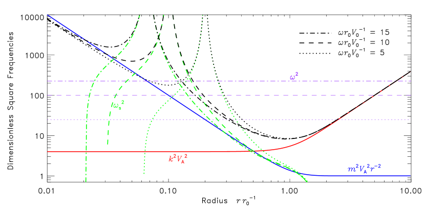
Figure 2: A propagation diagram that illustrates the radial cavity for the fast modes. The wave cavity exists wherever the waves are radial propagating, which corresponds to the range of radii where the wave frequency exceeds a critical frequency constructed by adding three special frequencies in quadrature $\omega^{2}>k^{2}V_{\rm A}^{2}+m^{2}V_{\rm A}^{2}\,r^{-2}+\omega_{s}^{2}$. The red curve corresponds to $k^{2}V_{\rm A}^{2}$ and the blue curve indicates $m^{2}V_{\rm A}^{2}\,r^{-2}$. The green curves show the square of the singular cut-off frequency, $\omega_{s}^{2}$, for the three dimensionless frequencies, $\omega r_{0}V_{0}^{-1}=5$, 10, and 15. See equation (3.15) for a definition of the cut-off frequency. The line style used for each frequency is indicated in the upper-right of the figure. The black curves indicate the critical frequencies obtained by adding the red, blue and green curves together. The squares of the three frequencies used to generate the cut-offs are indicated with the horizontal violet lines. All frequencies are generated for unit azimuthal order, $m=1$.

Figure 2 illustrates the special frequencies that define the wave cavity. All frequencies are nondimensionalized by $V_{0}r_{0}^{-1}$ and plotted in the form of their squares. The red curve corresponds to the quantity $k^{2}V_{\rm A}^{2}$ for an axial wavenumber of $kr_{0}=2$. The blue curve shows the square of the local Alfvén frequency $\omega_{A}^{2}=m^{2}V_{\rm A}^{2}/r^{2}$, which in these equations arises from the azimuthal wavenumber $m/r$ (and not from the Alfvén singularity). The three green curves represent the singular cut-off frequency for three different dimensionless frequencies, $\omega r_{0}V_{0}^{-1}=[5,10,15]$. The lowest frequency is shown by the dotted curve, the intermediate frequency by the dashed curve, and the highest frequency by the dot-dashed curve. The squares of the three wave frequencies are indicated with the horizontal violet lines using the same line styles. Finally, the critical frequency given by the sum of all three special frequencies, $\omega_{s}^{2}+\omega_{A}^{2}+k^{2}V_{\rm A}^{2}$, is shown using black curves. The cavity exists wherever the wave frequency (violet) exceeds the critical frequency (black).

From Figure 2 one can easily deduce that there is a single fast-wave cavity, bracketed by an inner and outer turning point. The outer turning point, $r_{2}$, is refractive and occurs where $\omega=kV_{\rm A}$. For the relatively high frequencies shown, the Alfvén speed is nearly a linear function of radius at the outer point and the outer turning point is therefore proportional to the axial phase speed of the wave,

$$r_{2}\to\frac{r_{0}}{V_{0}}\,\frac{\omega}{k}\;.$$ (3.16)

From this expression, we obtain the expected result that only waves that propagate at least partially in the axial direction are trapped. Purely radially propagating waves ($k=0$) are not refracted and therefore travel off to infinity.

The behavior of the inner turning point is more complicated. In the absence of the singularity, the fast wave would be excluded from the cylindrical origin by the geometrical effect of the azimuthal wavenumber, $m/r$ (the blue curve). However, in the presence of the singularity, the singular term dominates $\omega_{s}^{2}>>m^{2}V_{\rm A}^{2}/r^{2}$, and the inner turning point is moved outward and is largely dependent on the singularity. This means that the singularity occurs outside the fast-wave cavity, within the inner evanescence zone. Therefore, we should expect that the fast modes are inefficiently coupled to the Alfvén waves and only undergo weak damping. We will find that this expectation holds except for one noted exception.

An estimate for the inner turning point, $r_{1}$, can be obtained in the high-frequency limit by examining the behavior of the singular cut-off near resonance. For high frequencies, the Alfvén singularity approaches the origin. This can be verified by keeping only the first term in the power series expansion of the Lambert $W$-function, $W(x)=x-x^{2}+(3/2)x^{3}+\cdots$ to show that the Alfvén radius approaches

$$r_{A}\to m\,\frac{V_{0}}{\omega}\;.$$ (3.17)

In this limit, near the singularity, the square of the cut-off frequency is divergent and positive,

$$\omega_{s}^{2}\to\frac{1}{4}\frac{V_{0}^{2}}{\left(r-r_{\rm A}\right)^{2}}\;.$$ (3.18)

By combining the previous two equations and setting $\omega=\omega_{s}$, we find that the inner turning point is inversely proportional to frequency for high frequencies,

$$r_{1}\to\left(m+2\right)\frac{V_{0}}{\omega}\;.$$ (3.19)

4 Eigenspectrum

The eigenfunctions of equation (3.11) are those solutions that satisfy boundary conditions of regularity at the coordinate axis ($r=0$) and at infinity ($r\to\infty$). Appendix A provides a detailed discussion of the nature of the solutions at both boundaries. In short, the inner solution $\Phi_{0}$, i.e., the solution that is regular at the origin, behaves like a power law near the axis, $\Phi_{0}\sim r^{m}$. The outer solution, which is regular at infinity, behaves asymptotically like a modified Bessel function of the second kind, $\Phi_{\infty}\sim K_{\nu}(kr)$, with a frequency-dependent order, $\nu^{2}\equiv m^{2}-\omega^{2}r_{0}^{2}V_{0}^{-2}$. The eigenfunctions are the solutions that satisfy both regularity conditions and correspond to those frequencies and wavenumbers where the inner and outer solutions become linearly dependent (i.e., their Wronskian vanishes). After satisfying both boundary conditions, the eigenfunctions lack the necessary free parameters to also satisfy a regularity condition at the internal singularity associated with the Alfvén resonance $r=r_{\rm A}$. Hence, the solution is perforce irregular on the resonant field line.

In Appendix A.3, we present detailed derivations of the two solutions valid near the Alfvén resonances. Here we simply point out that one of the solutions is irregular and possesses a logarithmic singularity. A careful analysis of the irregular solution reveals that $\Phi$ itself is finite at the singularity, but the corresponding velocity field—obtained through equation (3.9)—is discontinuous and singular in both the radial and axial components. This poor behavior should be expected. A fast wave with a purely monochromatic frequency can be treated as if the wave has been resonantly transferring energy to the resonant field line for an infinite duration of time.

The eigenmodes correspond to the subset of frequencies and wavenumbers for which the Wronskian of the inner and outer solution vanishes,

$${\cal W}\left\{\Phi_{0},\Phi_{\infty}\right\}\left(r\right)=\Phi_{0}\frac{d{\Phi_{\infty}}}{d{r}}-\Phi_{\infty}\frac{d{\Phi_{0}}}{d{r}}=0\;.$$ (4.20)

Since our ODE has Sturm-Liouville form (albeit with a singular weight function), a more convenient description of the modal condition involves the dispersion function $D$ which is proportional to the Wronskian,

$$D\left(k,\omega\right)\equiv\frac{\cal{W}}{rK^{2}}=\frac{1}{rK^{2}}\left(\Phi_{0}\,\frac{d{\Phi_{\infty}}}{d{r}}-\frac{d{\Phi_{0}}}{d{r}}\,\Phi_{\infty}\right)=0\;.$$ (4.21)

The dispersion function, $D(k,\omega)$, has the useful property that it is independent of radius. This can be verified through direct differentiation, $dD/dr=0$, and use of the ODE (3.11).

In systems without damping, the modal condition $D(k,\omega)=0$ is rather straightforward. There are often a countable infinity of real zeros and one can consider either the frequency $\omega$ or the axial wavenumber $k$ as a real free parameter. Traditionally, one usually treats the wavenumber $k$ as the free parameter and the eigenvalues are discrete eigenfrequencies $\omega_{mn}(k)$ where the radial order $n$ is an integer that describes the number of nodes in the radial eigenfunction. Note, however, that it is equally valid to consider the frequency as the free parameter and the eigenvalues are eigenwavenumbers, $k_{mn}(\omega)$.

When the modes are damped, the eigenvalues becomes complex. Once again, it is traditional to think in terms of a continuous real wavenumber with a complex eigenfrequency $\omega_{n}(k)=\varpi_{n}(k)+i\gamma_{n}(k)$, where the dependence on the azimuthal order $m$ has been dropped from the notation. The real part of the eigenfrequency is inversely proportional to the wave period $P_{n}=2\pi/\varpi_{n}$, and the imaginary part defines the temporal damping rate $\gamma_{n}$. But as before, it is equally valid to consider real frequencies and complex eigenwavenumbers, $k_{n}(\omega)=\kappa_{n}(\omega)+i\eta_{n}(\omega)$. Here, the real part of the complex wavenumber is related to the wavelength $\lambda_{n}=2\pi/\kappa_{n}$ and the imaginary part is the spatial decay rate, $\eta_{n}$. Usually it does not matter which viewpoint one adopts; however, in this case the perverse nature of the internal singularity actually makes the latter view more fruitful. We discuss this issue in more detail in Appendix B.

4.1 Numerical Solutions

We numerically solve for the inner and outer solutions (and hence the dispersion function) by using a somewhat complicated shooting technique. For the inner solution $\Phi_{0}$ we start our numerical integrations at a small radius, $r_{\rm in}<<\inf(r_{0},r_{\rm A})$, and obtain $\Phi_{0}(r_{\rm in})$ and its derivative by using a power-series expansion that is valid near the origin (see Appendix A.1). Then, using a 5th-order, adaptive-stepsize, Runge-Kutta algorithm, we numerically integrate equation (3.11) from $r_{\rm in}$ to any chosen radius $r=R$. When evaluating the dispersion function the actual value of $R$ that is chosen is immaterial since the dispersion function is independent of radius. If $R<r_{\rm A}$, this desired radius lies inside the Alfvén resonance and we do not need to explicitly worry about the interior singularity. However, if $R>r_{\rm A}$ we need to integrate through the singularity and this, of course, requires some care.

When the singularity lies between the origin and the desired radius $R$, we match the inner solution to a linear combination of the solutions that are regular $\Phi_{\rm reg}$ and irregular $\Phi_{\rm irr}$ at the Alfvén singularity,

$$\Phi=A_{\rm reg}\Phi_{\rm reg}+A_{\rm irr}\Phi_{\rm irr}\;.$$ (4.22)

This is accomplished by exploiting power-series expansions for $\Phi_{\rm reg}$ and $\Phi_{\rm irr}$ that are valid near the interior singular point (see Appendix A.3). Each expansion is evaluated just inside the singularity, i.e., at $r=r_{A}-\delta$ where $\delta$ is positive and small. This provides a starting point for the numerical integrations. Then using the same Runge-Kutta integrator, we numerically integrate both solutions from $r=r_{A}-\delta$ to a point half-way between the origin and the Alfvén singularity, $r=r_{\rm A}/2$. The inner solution $\Phi_{0}$ is then integrated from $r_{\rm in}$ near the origin to the same point. The connection coefficients, $A_{\rm reg}$ and $A_{\rm irr}$, are chosen to ensure that the inner solution $\Phi_{0}$ and the solution initially generated near the singularity match cleanly (their functions and their derivatives match). Once computed these connection coefficients can subsequently be used to generate the inner solution on the far side of the singularity by using the power-series expansions to evaluate $\Phi_{\rm reg}$ and $\Phi_{\rm irr}$ at $r=r_{A}+\delta$. This solution (comprised of the linear combination of regular and irregular solutions) is then numerically integrated to the desired radius $R$. We use a similar procedure to numerically evaluate the outer solution. The only difference is that the starting radius is large, $r_{\rm out}>>\sup(r_{0},r_{\rm A})$, and an asymptotic solution that is valid for large radius is used to initiate the numerical integrations (see Appendix A.2).

4.2 Dispersion Function

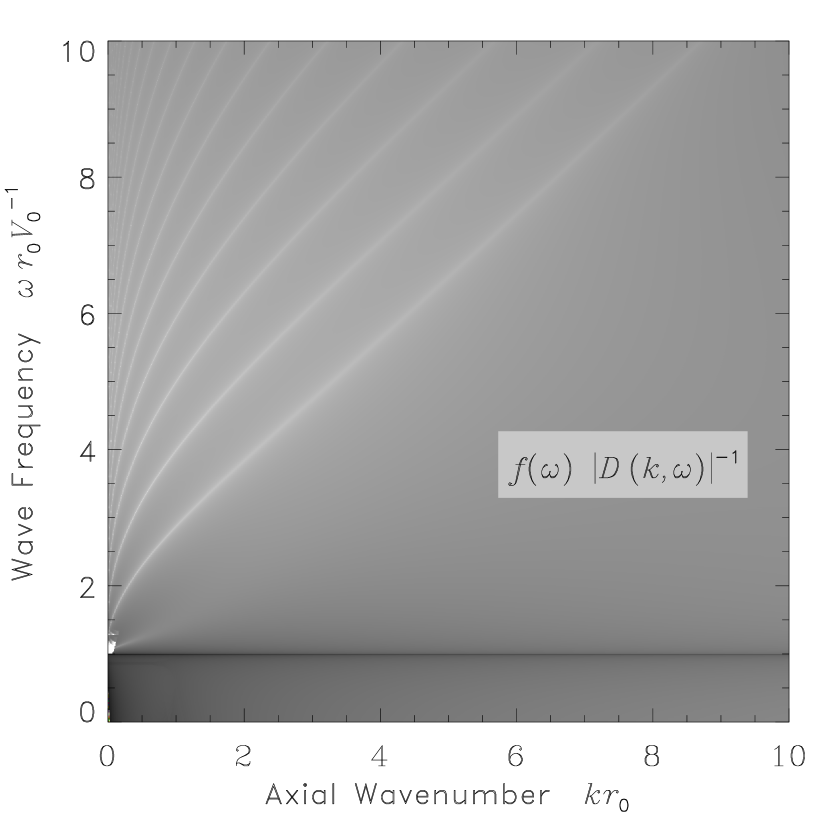
Figure 3: The reciprocal of the modulus of the dispersion function multiplied by a function of frequency, $f(\omega)\,|D(k,\omega)|^{-1}$, is displayed as a function of real dimensionless wavenumber $kr_{0}$ and frequency $\omega r_{0}V_{0}^{-1}$. The azimuthal order is unity, $m=1$. The function of frequency was chosen solely to remove a strong gradient in frequency from the image, $f(\omega)=\exp\left(-0.2\;\omega r_{0}V_{0}^{-1}\right)$. The eigenmodes correspond to the bright ridges where the dispersion function is nearly zero. The dark horizontal band lies at a frequency $\omega=mV_{0}/r_{0}$ which corresponds to the frequency where the Alfvén resonance has moved to an infinite radius. All eigenmodes exist above this frequency bound. The lowest frequency mode (i.e., the ridge with the lowest radial order) is heavily damped and visible only at low wavenumbers ($kr_{0}<1$). At higher wavenumbers, this mode’s line profile becomes sufficiently wide that the mode disappears into the background. The sharp-edged, bright feature near $\omega r_{0}V_{0}^{-1}=m$ at very low wavenumber ($kr_{0}<0.1$) is a numerical artifact caused by the necessity of solving the equations in a finite radial domain.

Figure 3 illustrates the numerically computed dispersion function and its variation with the spectral parameters $k$ and $\omega$ for the fundamental azimuthal order $m=1$. The frequency and wavenumber dependence are characterized with a dimensionless frequency $\omega\,r_{0}V_{0}^{-1}$ and a dimensionless wavenumber $kr_{0}$. A smooth gradient in frequency has been removed from the image for purely illustrative purposes. This has been accomplished by multiplying the reciprocal of the dispersion function by a pure function of frequency, $f(\omega)=\exp\left(-0.2\;\omega\,r_{0}V_{0}^{-1}\right)$. One can clearly recognize the presence of strong fast-mode resonances which appear as bright “ridges” of high power. As we will soon see, each ridge corresponds to resonant fast waves with differing number of peaks in the modulus of their eigenfunctions as a function of radius. The lowest-frequency ridge has one peak in its eigenfunction and we designate its radial order as $n=0$. Each ridge of sequentially higher frequency has one additional peak and a corresponding radial order of one higher, i.e., $n=1$, 2, 3, and so forth. Traditionally, the radial order of a mode (or ridge) specifies the number of radial nodes in its eigenfunction. However, because of resonant absorption, our eigenfunctions are complex and lack nodes where both the real and imaginary part vanish. Therefore, we use the number of maxima in the modulus of the eigenfunction instead. The radial order $n$ is defined to be one less than the number of peaks.

These radial resonances arise from waves trapped between two radial turning points. The outer turning point is caused by refraction from the increasing Alfvén speed with height. The inner turning point is due to the combined effect of reflection from the Alfvén singularity and from the geometrical increase in the azimuthal wavenumber $m/r$ for small radii. For a given radial order, the frequency approaches a nonzero value as the axial wavenumber approaches zero. This is due to the asymptotic form of our Alfvén speed profile for large radius. Refraction requires oblique propagation and waves that propagate purely radially $k=0$ are unrefracted and untrapped. Hence as the axial wavenumber $k$ approaches zero, the outer turning point approaches infinity and the radial wavelength becomes infinity large. Since the cavity extends to large radii, the Alfvén speed is nearly a linear function throughout most of the wave cavity, $V_{\rm A}\approx V_{0}\,r/r_{0}$. Using this asymptotic form, equation (3.14) reveals that the wave’s frequency must approach a finite value as $k$ vanishes, $\omega\to mV_{0}r_{0}^{-1}$.

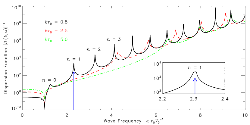
Figure 4: Three cuts at constant wavenumber through the reciprocal of the modulus of the dispersion function shown in Figure 3. The black solid curve illlustrates the dispersion function for a low wavenumber, $kr_{0}=0.5$ and the dashed red and dot-dashed green curves show successively higher wavenumbers, $kr_{0}=2.5$ and $5.0$ respectively. The $n=1$ mode, indicated with the blue arrow, is shown in a zoom-in view in the inset.

All of the modes are damped due to resonant absorption by the Alfvén waves and hence have complex eigenfrequencies or wavenumbers. Thus, for real frequency and real wavenumber (as shown in the figure), the dispersion function is never truly zero. Instead, as the frequency and wavenumber pass near a complex zero in the dispersion function, the power peaks with a Lorentzian profile. The width of the profile is a direct measure of the damping rate. Figure 4 shows cuts through the reciprocal of the dispersion function at three representative values of the axial wavenumber. Each ridge appears as a large amplitude Lorentzian spike. This profile shape is revealed in the inset where the mode marked with the blue arrow is shown over a narrow range of frequency.

The lowest radial-order ridge in the power spectrum illustrated in Figure 3 spans only a short range of wavenumbers before it fades into the background. This ridge appears near a nondimensional frequency of $\omega r_{0}V_{0}^{-1}=m=1$ in the lower-left corner of the power spectra. This short feature of high power corresponds to the fundamental radial order $n=0$. As we will see, this mode is strongly damped by resonant absorption and at higher wavenumbers ($kr_{0}>1$), the ridge widens so much in spectral space that it becomes indistinguishable from the background. When we examine eigenfunctions in detail in the next section, we will find that the energy density of the fundamental radial mode has a single extremum located at the Alfvén singularity. Each ridge of successively higher frequency and radial order ($n=1$, $n=2$, $n=3$, and so forth) adds an additional peak to the energy density as a function of radius. These radial overtones are only weakly damped and thus have narrow ridges and the power varies by orders of magnitude between the inter-ridge background and the ridge peaks (see Figure 4).

Due to the fact that we solve the ODEs by Runge-Kutta integration, we expect that numerical inaccuracies should arise when we must integrate very long distances. The region of spectral space near the low-wavenumber base of the lowest-frequency ridge is a region where such long integrations become necessary. This numerical difficulty arises for two compounding reasons. As the dimensionless frequency approaches $m$ the resonant field line moves infinitely far away in radius. Similarly, the outer refraction point or turning point, $r_{2}$, of the fast wave moves farther and farther away from the axis as the wavenumber becomes small, $r_{2}\approx r_{0}V_{0}^{-1}\,\omega/k$. For both reasons, as the axial wavenumber vanishes and the dimensionless frequency approaches $m$, we must move the outer boundary of our computational domain, $r_{\rm out}$, further and further away. This means that our numerical integrations must cross longer and longer distances and as numerical errors accumulate, these long distance integrations become increasingly inaccurate. In the very small spectral region at the base of the $n=0$ ridge where this inaccuracy becomes unacceptable, we saturate the image with pure white.

4.3 Eigenwavenumbers

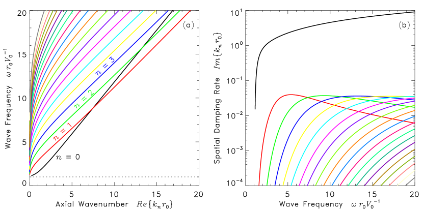
Figure 5: (a) Real and (b) imaginary parts of the eigenwavenumber displayed as a function of frequency for $m=1$. Each color curve corresponds to a different radial order, with black indicating the fundamental radial order, $n=0$. Higher radial orders are illustrated with red ($n=1$), green ($n=2$), blue ($n=3$), and so on. The fundamental radial order has a different asymptotic slope for large wavenumber than the higher radial orders. Further, the spatial damping rate for the fundamental radial order is much larger. Note, even though the dispersion relation (panel a) for the fundamental mode crosses those of higher order, this is not an avoided crossing because the eigenwavenumbers are complex and the modes have distinct imaginary parts. The dotted horizontal line indicates the dimensionless frequency equals $m$.

We find the complex eigenwavenumbers using a complex root finder that utilizes a numerical routine which calculates the dispersion function for any requested frequency and wavenumber. At a given frequency, the root finder starts from an initial guess for the eigenwavenumber and iterates until it converges to a complex zero in the dispersion function. Figure 5 shows the real and imaginary parts of the resulting axial wavenumber as a function of position along each ridge. The black curve corresponds to the fundamental radial mode ($n=0$) and the sequence of colored curves is a sequence of radial order $n$ (red: $n=1$, green: $n=2$, blue: $n=3$, etc.). Figure 5$a$ shows the dispersion relation, i.e., the frequency as a function of the real part of the wavenumber, while Figure 5$b$ shows the spatial damping rate (the imaginary part of the wavenumber) as a function of frequency. Since, the eigenwavenumber, $k_{n}(\omega)$, only appears as its square $k_{n}^{2}$ in the ODE (3.11), for each eigenvalue there are a pair of solutions $\pm\sqrt{k_{n}^{2}}$, one corresponding to forward-propagating waves (i.e., phase moves in the positive $y$-direction) and the other to backward propagating waves. Since the two solutions have the same radial eigenfunction, we only show the forward-propagating wave with a positive real part of its eigenwavenumber.

The radial overtones ($n>0$) all have dispersion relations and spatial damping rates with similar behavior. As the frequency increases, the real part of the wavenumber increases, initially quite quickly, and then approaches a slope common to all overtones. The spatial damping rate of all overtones is quite small and peaks at a frequency that depends on the radial order. Interesting, the dimensionless damping rate for all radial orders peaks at roughly the same value, $\sim 4\times 10^{-2}$. The radial fundamental mode ($n=0$) behaves discordantly. The dispersion relation is convex instead of concave and asymptotically approaches a steeper slope than the overtones. More importantly, the fundamental mode is heavily damped. Resonant absorption produces a spatial decay rate that is orders of magnitude larger than that evinced by the overtones.

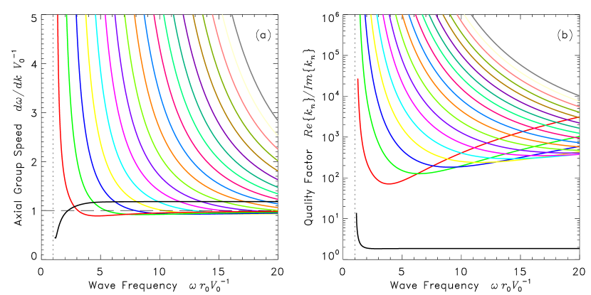
Figure 6: (a) Axial group speed and (b) quality factor for the eigenmodes as a function of dimensionless frequency and radial order. The azimuthal order is unity, $m=1$. The colors have the same meaning as in Figure 5. The group velocity is defined as the slope of the curves in Figure 5a. Asymptotically for high frequency, the group speed approaches a constant. For the radial overtones ($n>0$), this asymptotic value is equal to the Alfvén speed at the axis, $V_{0}$. For the fundamental mode, the asymptotic value is somewhat higher. The quality factor, $Q$, is the ratio of the real to imaginary parts of the eigenwavenumber and signifies the number of wavelengths the wave travels before it is significantly diminished in amplitude. The fundamental mode is heavily damped and travels only a few wavelengths before being absorbed ($Q\sim 2$). The radial overtones are all weakly damped ($Q>100$) and the quality factor achieves a minimum at a frequency that increases as the order increases.

Figure 6a shows the axial group speed, $v_{\rm grp}$, of each radial order as a function of frequency,

$$\frac{1}{v_{\rm grp}}\equiv Re\left\{\frac{\partial{k_{n}}}{\partial{\omega}}\right\}\;.$$ (4.23)

The overtones ($n>0$) behave as one would expect. Waves with low axial wavenumber propagate outward nearly radially and refract back toward the axis at a turning point located at large radius. Such waves sample regions with high Alfvén speed and thus have a high axial group speed. As the frequency and wavenumber increase, the turning point moves inward, confining the mode to the region of low Alfvén speed near the axis. Hence, the group speed asymptotically approaches a value of $V_{0}$ as the frequency increases. The radial fundamental modes defies this trend. Its group speed increases with frequency and approaches a constant value that is larger than $V_{0}$.

The magnitude of the spatial damping rate can be put into context by considering the quality factor $Q$ which is defined as the ratio of the real and imaginary part of the eigenvalue,

$$Q\equiv\frac{Re\left\{k_{n}\right\}}{Im\left\{k_{n}\right\}}\;.$$ (4.24)

The quality factor is a measure of the number of wavelengths that the wave travels before it suffers significant attenuation. The quality factor for each radial order is shown in Figure 6b. The overtones are all weakly damped and travel hundreds of wavelengths before significant amplitude decay occurs. As such, the quality factor for these modes exceeds 100 for all frequencies. On the other hand, the radial fundamental mode has a quality factor of nearly 2 at almost all frequencies. This wave only travels a single wavelength before losing most of its energy through resonant coupling with the Alfvén waves.

4.4 Eigenfunctions

The eigenfunctions can be generated by evaluating the outer solution at the eigenwavenumber,

$$\Phi_{mn}(r\,|\,\omega)=\Phi_{\infty}(r\,|\,k_{n}(\omega),\omega)\;.$$ (4.25)

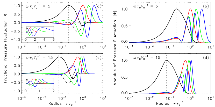
Figure 7: The fractional magnetic-pressure fluctuation, $\Phi_{mn}(r\,|\,\omega)$, as a function of radius, for the eigenfunctions of the first four radial orders and for $m=1$. The different colors of the curves indicate the radial order (black: $n=0$, red: $n=1$, green: $n=2$, and blue: $n=3$). In all panels the vertical dotted line indicates the radius at which the Alfvén singularity occurs for the given frequency. (a) The pressure eigenfunctions for a dimensionless frequency of $\omega r_{0}V_{0}^{-1}=5$. The solid curves display the real part of the complex eigenfunction and the dashed-curve shows the imaginary part for the radial fundamental ($n=0$). The imaginary parts of the other orders have been omitted since their eigenfunctions are nearly real due to weak damping. The inset shows the real part of the eigenfunctions on a linear radius scale. (b) The modulus of the complex eigenfunctions. From this figure one can easily recognize that the radial order indicates the number of peaks appearing in the modulus (e.g., $n=0$ has 1 peak, $n=1$ has 2 peaks and so forth). (c) Pressure fluctuation for eigenfunctions with a dimensionless frequency of $\omega r_{0}V_{0}^{-1}=15$. The eigenfunctions all have the same structure as those at lower frequency, but are compressed towards the origin. (d) The modulus of the eigenfunctions for the higher frequency.

Figures 7a and c illustrate the fractional magnetic-pressure fluctuation for eigenfunctions with radial orders $n\leq 3$ for two different frequencies. The color of the curves indicates the eigenmode’s radial order (see the caption). As the radial order increases, the axial wavelength of the mode increases (see Figure 5) and the wave refracts at a larger radius where the Alfvén speed is larger. Thus, the higher-order overtones have eigenfunctions with larger wave cavities that extend higher in radius. To capture this increase in size of the wave cavity in a common figure, we have plotted the eigenfunctions using a logarithmically scaled radius axis. A linear scaling is also provided in a small inset. All eigenfunctions are complex quantities because of the damping caused by resonant absorption. However, the damping is exceedingly weak for all modes other than the radial fundamental mode. Thus, only the $n=0$ mode has a significant imaginary component. The real part of each eigenfunction is displayed using solid curves and the imaginary part of the fundamental is shown with a dashed curve. Since the eigenfunctions are complex, it is not obvious that the radial order indicates the number of nodes in the eigenfunction. However, if we examine the modulus of the eigenfunctions, as illustrated in figures 7b and d, the trend becomes clear. The modulus of each complex eigenfunction has a number of peaks in radius equal to $n+1$. Thus, even though the radial fundamental mode has an eigenfunction with significant real and imaginary parts, and those parts may separately have nodes, the modulus is singly lobed with one extrema.

From the power series expansions of the two solutions valid at the singularity (see Appendix A.3), one can easily determine that the pressure fluctuation, $\Phi$, remains finite and has vanishing derivative. The regular solution and its derivative both vanish, so the solution is dominated by the irregular solution

$$\Phi\,\propto\,\Phi_{\rm irr} = 1+\frac{k^{2}r_{0}^{2}}{2}\,(r-r_{\rm A})^{2}\ln(r-r_{\rm A})+\cdots\to 1\;,$$ (4.26)

$$\frac{d{\Phi}}{d{r}}\,\propto\,\frac{d{\Phi_{\rm irr}}}{d{r}} = k^{2}r_{0}^{2}\,(r-r_{\rm A})\ln(r-r_{\rm A})+\cdots\to 0\;.$$ (4.27)

From these two expansions, we immediately deduce that the Alfvén radius must be a local peak in the eigenfunction. This prediction is born out in an examination of the numerically calculated eigenfunctions presented in Figure 7. The influence of the Alfvén singularity essentially adds an additional peak to all of the eigenfunctions of the fast modes. This suggests that the $n=0$ mode (with only a single peak at the Alfvén singularity) only exists because of the presence of the singularity. The radial fundamental mode has a different physical origin than the higher radial orders.

While the magnetic-pressure fluctuation remains finite at the singularity, the velocity components of the eigenfunction do not. From the leading-order behavior at the singularity, equation (3.9) indicates that both the axial and radial velocity are singular,

$$u_{y}=\frac{V_{\rm A}^{2}}{\omega^{2}-\omega_{\rm A}^{2}}\;ik\Phi \sim \frac{1}{r-r_{\rm A}}+\cdots\;,$$ (4.28)

$$u_{r}=\frac{V_{\rm A}^{2}}{\omega^{2}-\omega_{\rm A}^{2}}\;\frac{d{\Phi}}{d{r}} \sim k^{2}r_{0}^{2}\,\ln(r-r_{\rm A})+\cdots\;.$$ (4.29)

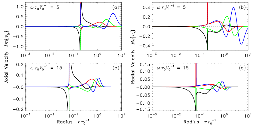
Figure 8: The velocity eigenfunctions for the same modes illustrated in Figure 7. The colors have the same meaning as in that figure. The left-hand panels (a) and (c) display the imaginary part of the axial velocity component and the right-hand panels (b) and (d) present the real part of the radial velocity component. The upper panels show a small frequency and the lower panels show a large frequency. Both velocity components are complex quantities, but for the radial overtones (which have weak damping), the axial component is almost purely imaginary and the radial component is nearly real. All velocity components are singular at the Alfvén radius (which is indicated by the vertical dotted line). The axial velocity component has a hyperbolic divergence, $\sim 1/(r-r_{\rm A})$ while the radial component has a logarithmic divergence $\sim\log(r-r_{\rm A})$.

Figure 8 illustrates both of these velocity components. When the fractional magnetic-pressure fluctuation, $\Phi$, is purely real, the axial velocity is purely imaginary and the radial velocity is purely real. Hence, in Figure 8 we display the imaginary part of the axial velocity and real part of the radial velocity.

5 Discussion

The dispersion relation and spatial damping rate (see Figures 6a,b) clearly demonstrate that radial fundamental mode ($n=0$) has a very different physical nature than all of the higher order radial modes. We reiterate that the radial fundamental only exists because of the singularity. If we were to slowly perturb the Alfvén speed profile to one where the singularity vanished (for example $V_{\rm A}\propto r$), the radial fundamental mode would also disappear, while the overtones would remain.

5.1 Wave Cavities

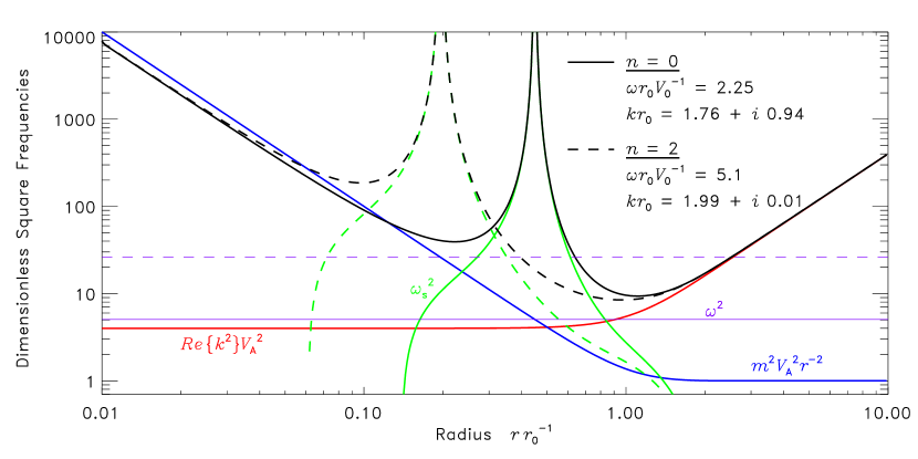
Figure 9: A propagation diagram illustrating that the fundamental radial mode is a fast surface wave, whereas the radial overtones are fast body waves. Two particular modes with $m=1$ are presented. The solid curves are those for a $n=0$ mode with a dimensionless frequency of 2.55 and a complex wavenumber of $kr_{0}=1.76+i\,0.94$. The dashed curves are for a $n=2$ mode with a frequency of 5.1 and wavenumber of $kr_{0}=1.99+i\,0.01$. Both modes have $Re\left\{k^{2}\right\}=4.0$. Thus the solid red and blue curves show common values for the frequencies $kV_{\rm A}$ and $mr^{-1}V_{\rm A}$. The two horizontal violet curves indicate the two mode frequencies. For the $n=2$ mode, it is clear that there exists a range of radii for which the frequency exceeds the critical frequency and there exists a cavity where the wave propagates. The overtone is therefore primarily a body wave. The fundamental radial mode ($n=0$) has a frequency that nowhere exceeds the critical frequency. Hence is must be a surface wave that exists on the only discontinuity present, the Alfvén singularity.

The disparate behavior between the fundamental radial mode and the radial overtones is primary due to the fact that the overtones reside in a fast wave cavity whereas the fundamental is a surface wave that resides on the singularity. All of the overtones ($n>0$) have frequencies that are sufficiently high that they possess a cavity where the wave is propagating as indicated in Figure 2. Thus, the overtones are all primarily fast body waves. Further, the Alfvén singularity lies just inside the inner turning point and thus lies outside of the fast wave cavity. This explains why the the resonant coupling between the overtones and the Alfvén waves is inefficient and the overtones are weakly damped. The singularity lies in the evanescent tail of the overtones where the mode’s amplitude is relatively low. The radial fundamental $n=0$ on the other hand is nowhere propagating and lacks a fast wave cavity. Figure 9 provides a propagation diagram for two modes $n=0$ and $n=2$. Both have eigenvalues $k^{2}$ with identical real parts, $Re\left\{k^{2}\right\}=4.0$. Of course, they have different frequencies and different imaginary parts of their eigenvalues. Nowhere does the fundamental have a frequency that exceeds the critical frequency. Thus, this mode is a surface wave that lives on the only available discontinuity, the Alfvén singularity. Since this mode’s energy density is concentrated at the singularity, resonant absorption is efficient.

5.2 Restoring Forces

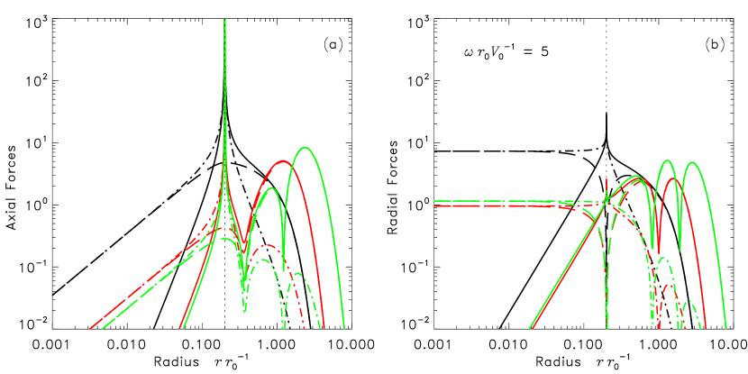
Figure 10: The magnitudes of the two restoring forces, magnetic pressure and magnetic tension, in (a) the axial direction and (b) the radial direction. The black curves indicate the forces for the radial fundamental mode $n=0$, while the red and green curves indicate the first two overtones, $n=1$ and $n=2$ respectively. All forces are for modes with the same nondimensional frequency, $\omega r_{0}V_{0}^{-1}=5$, and azimuthal order, $m=1$. The modulus of the magnetic pressure force is illustrated with the dashed curves and the modulus of the tension with the dot-dashed curves. The modulus of the total restoring force (pressure plus tension) is shown with solid curves. Clearly, the magnetic pressure dominates over most of the wave cavity. The only exceptions are at the Alfvén singularity (indicated with the vertical dotted line) and near the origin. Near the singularity, the magnetic tension dominates. Near the origin the two forces have the same magnitude but are almost 180 degrees out of phase such that they nearly cancel when summed.

Fast waves have two potential restoring forces that usually act in concert, magnetic pressure and magnetic tension. Figure 10 illustrates the magnitudes of these two forces for three modes of different radial order but the same frequency. A careful examination of the restoring forces in both the axial and radial directions reveals that the magnetic pressure dominates everywhere except at the Alfvén singularity and near the origin. At the singularity magnetic tension becomes the most important force. Near the origin, the tension and pressure are of equal magnitude but nearly 180 degrees out of phase such that they nearly cancel each other. Since the overtones have radial cavities that extend well-above the Alfvén singularity, over most of the region where the mode has significant amplitude, the magnetic pressure is the primary restoring force. Hence, the overtones are primarily fast pressure waves with weak contributions from the tension. The radial fundamental mode on the other hand has an eigenfunction that is confined to the immediate vicinity of the singularity. Thus, not only is the fundamental primarily a fast tension wave with weak pressure contributions, its suffers extensive resonant absorption because it is confined to a region of strong coupling.

5.3 Observational Implications

Our assumption that the axial direction is infinite and ignorable is not trivial. The primary effect is that all axial wavenumbers are allowed because of the infinite domain. This allows us to consider the axial wavenumber as a “radial eigenvalue” and the frequency as a free-parameter. On the other hand, if there were boundaries placed along the axial coordinate, the wavenumber would be quantitized and fixed in order to satisfy the axial boundary conditions. This would require that the frequency represent the radial eigenvalue.

For most of the fast modes this is a serious constraint. They have such low damping rate arising from resonant absorption that they can travel very far before having their signal attenuated. For example, if we consider a model arcade with a typical length scale of $r_{0}=100$ Mm, the smallest spatial decay length for the overtones is roughly $r_{0}/(4\times 10^{-2})=2500$ Mm. Assuming a typical arcade whose length is on the order of a solar radius, these waves would sense both boundaries. Thus, they would bounce back and forth multiple times before being dissipated. The low-amplitude “decayless oscillations” may be the result of such fast wave oscillations. One or more excitation events generate a set of radial overtones that interfere with each other and with themselves as they criss-cross the axial cavity.

The radial fundamental mode is different. This mode only travels a few wavelengths before significant decay occurs. Thus, this mode would die before reaching the edges of a long arcade and its axial wavenumber would not be quantitized to an obvious degree. Once excited these waves would dissipate rather quickly into Alfvén waves and would never travel far from where they were generated. Thus, the radial fundamental mode can only be observed as coronal loop oscillations if those oscillations are excited locally.

Loop oscillations have to date only been observed by their motion on the plane of the sky. Thus, what is observed is a linear combination of the two transverse velocity components, and observed polarization depends on the angle between the line of sight and the arcade’s axis. The eigenfunction for either velocity component is singular at the Alfvén radius. Note, however, this singularity should never be observed, as a pure eigenmode is never excited. Instead, all physically realizable wave fields are composed of a linear combination of eigenfunctions represented by an integral over frequency. Each frequency component in the integration has a singularity at a different radius. So, even though the integrand has singularities the integral must remain finite at all radii. For wave packets comprised of a narrow band of frequencies we expect a large, but finite, radial response at the Alfvén radius concomitant with the central frequency of the band. But, the wave packet may also have a significant response at higher radii corresponding to peaks in the amplitude of the velocity eigenfunctions if the packet possesses radial overtones in its makeup. The motion of a single coronal loop, however, will only reveal the motion at a single shell or magnetic surface. It could very well be that the largest field line displacements remain invisible if the radius of the observed loop does not coincide with the Alfvén radius for the dominant frequency of the excited waves.

Appendix A Solutions near the Singular Points

The governing ODE (3.11) has three (or more) singular points in radius: the origin ($r=0$), infinity ($r\to\infty$), and one or more Alfvén resonances ($r=r_{\rm A}$). For monotonic Alfvén frequency profiles, like that which arises from equation (2.2) and illustrated in Figure 1, there is at most a single Alfvén radius for any particular frequency. The solutions that are regular at the origin and at infinity can be obtained through standard expansions and asymptotic analyses. As such, they will be discussed here only briefly. The interior singularity at the Alfvén radius is more unusual and warrants a more detailed examination.

A.1 Solution near the Origin

A power-series solution to equation (3.11) that is valid near the origin can be found by expanding the square of the local wavenumber, $K^{2}$, in an expansion for small radius, $r<<\inf\left(r_{0},\,k^{-1}\right)$, and using the method of Frobenius to build the series solution term by term. To lowest order, the two solutions to equation (3.11) behave like $r^{\pm m}$. We present the first few terms in the power series for the regular, well-behaved solution,

$$\Phi_{0}\left(r\,|\,k,\omega\right) = (r/r_{0})^{m}\left[1+a_{2}(r/r_{0})^{2}+a_{4}(r/r_{0})^{4}+\cdots\right]\;$$ (A1)

$$a_{2} = -\frac{\Omega^{2}-k^{2}r_{0}^{2}+2m\alpha}{4(m+1)}\;$$ (A2)

$$a_{4} = -\frac{\Omega^{2}-k^{2}r_{0}^{2}+2(m+2)\alpha}{8(m+2)}\;a_{2}+2m\alpha\;\frac{(m+4)q_{2}-2\alpha}{16(m+2)}\;,$$ (A3)

$$\Omega \equiv \frac{\omega r_{0}}{V_{0}}\;,\;\;\;\;\alpha\equiv\frac{\Omega^{2}}{m^{2}}\;,\;\;\;\;q_{2}\equiv\frac{r_{0}^{2}}{2!V_{0}^{2}}\left.\frac{d^{2}{V_{A}^{2}}}{d{r}^{2}}\right|_{r=0}\;.$$ (A4)

A.2 Asymptotic Solution for Large Radius

In the limit of large radius, $r>>\sup\left(r_{0},\,k^{-1}\right)$, the outer solution $\Phi_{\infty}$ behaves like a modified Bessel function. This can be verified by recognizing that $V_{\rm A}\to V_{0}(r/r_{0})$ and the ODE (3.11) becomes Bessel’s equation (Hindman & Jain, 2015),

$$\frac{d^{2}{\Phi_{\infty}}}{d{r}^{2}}+\frac{1}{r}\frac{d{\Phi_{\infty}}}{d{r}}-\left(\frac{\nu^{2}}{r^{2}}+k^{2}\right)\Phi_{\infty}=0\;,$$ (A5)

where we define the constant $\nu^{2}\equiv m^{2}-\Omega^{2}$. The solution that is well-behaved for large radius is the $K$ function (modified Bessel function of the second kind),

$$\Phi_{\infty}(r\,|\,k,\omega)\to K_{\nu}(\pm kr)\;,$$ (A6)

where the sign of the argument is chosen to ensure that the real part is positive (otherwise the solution diverges exponentially for large $r$).

In order to use the asymptotic solution to initialize the numerical integrations in our analysis (and hence satisfy the radial boundary condition at infinity), we need to be able to evaluate the $K$ Bessel function for complex frequencies and wavenumbers. Complex frequencies impose complex azimuthal orders, $\nu$, and complex wavenumbers impose complex arguments. Most standard Bessel function algorithms are incapable of dealing with these complications. Hence, we use an asymptotic expansion that is valid for large values of the argument,

$$\Phi_{\infty}(r\,|\,k,\omega)=\sqrt{\frac{\pi}{2kr}}\;e^{-kr}\;\sum_{n=0}^{N-1}\frac{b_{n}}{n!(8kr)^{n}}\;,$$ (A7)

with coefficients given by

$$b_{0} \equiv 1\;,$$ (A8)

$$b_{n} \equiv \left[4\nu^{2}-(2n-1)^{2}\right]\,b_{n-1}\;\;\;{\rm for}\;\;n>0\;.$$ (A9)

The number of terms $N$ is chosen to optimize the accuracy of the expansion and the radius at which to initiate the integration is chosen to ensure a minimal degree of accuracy.

A.3 Solution near the Alfvén Singularity

The Alfvén resonances ($r=r_{\rm A}$) are interior singularities that are logarithmic regular singular points (e.g., Uberoi, 1972; Appert et al., 1974; Goedbloed, 1971), much like the origin in Bessel’s equation. The two solutions are therefore a regular, well-behaved solution $\Phi_{\rm reg}$ and an irregular solution $\Phi_{\rm irr}$ with a logarithmic singularity. Both will be needed. Through a Frobenius expansion around the singularity, one can obtain expansion coefficients. The series are written in terms of a nondimensional local coordinate $\varepsilon=(r-r_{\rm A})/r_{0}$. The first handful of terms are as follows

$$\Phi_{\rm reg}(r\,|\,k,\omega) = \varepsilon^{2}+\frac{2}{3}\,A_{0}\,\varepsilon^{3}+\frac{1}{4}\left(A_{0}^{2}-A_{1}-\frac{k^{2}r_{0}^{2}}{2}\right)\,\varepsilon^{4}+O\left(\varepsilon^{5}\right)\;,$$ (A10)

$$\Phi_{\rm irr}(r\,|\,k,\omega) = \frac{k^{2}r_{0}^{2}}{2}\,\Phi_{\rm reg}\,\ln\left(\varepsilon\right)+1-\frac{1}{6}\left(\frac{5}{6}A_{0}+\Lambda^{\prime}(0)\right)\varepsilon^{3}+O\left(\varepsilon^{4}\right)\;,$$ (A11)

where the primes denote differentiation with respect to $\varepsilon$ and the following definitions have been made,

$$\Lambda(\varepsilon) \equiv r_{0}^{2}\,K^{2}=r_{0}^{2}\;\frac{\omega^{2}-\omega_{A}^{2}}{V_{\rm A}^{2}}\;,$$ (A12)

$$A_{0} \equiv \frac{\Lambda^{\prime\prime}(0)}{2\Lambda^{\prime}(0)}+\frac{r_{0}}{r_{\rm A}}\;,$$ (A13)

$$A_{1} \equiv \frac{\Lambda^{\prime\prime\prime}(0)}{3\Lambda^{\prime}(0)}-\left(\frac{\Lambda^{\prime\prime}(0)}{2\Lambda^{\prime}(0)}\right)^{2}-\left(\frac{r_{0}}{r_{\rm A}}\right)^{2}\;.$$ (A14)

In developing these series expansions, we have assumed that the derivative of the local Alfvén frequency is nonzero at the singularity such that to lowest order $\omega^{2}-\omega_{A}^{2}\sim\varepsilon$ (or equivalently, $\Lambda^{\prime}(0)\neq 0$).

The regular solution, as well as its radial derivative, vanishes at the singularity. From this condition and from a slight rearrangement of equation (3.9),

$${\mbox{{\boldmath$u$}}}=\frac{V_{\rm A}^{2}}{\omega^{2}-\omega_{A}^{2}}{\mbox{{\boldmath$\nabla$}}}_{\perp}\Phi\;,$$ (A15)

we can deduce that all physical variables (i.e., the magnetic pressure and both velocity components) vanish at the singularity. On the other hand the irregular solution possesses a “buried” logarithmic singularity. By buried we mean that the pressure variable and its first derivative remain continuous and finite, whereas its second derivative is singular (i.e., $\Phi_{\rm irr}$ is a $C^{1}$ function). In terms of the physical variables, the magnetic pressure is well-behaved, but both velocity components are divergent,

$$\Phi_{\rm irr} = 1+\frac{k^{2}r_{0}^{2}}{2}\,\varepsilon^{2}\,\ln\varepsilon+\cdots\;,$$ (A16)

$$u_{{\rm irr},r} = \frac{k^{2}r_{0}^{3}}{\Lambda^{\prime}(0)}\;\ln\varepsilon+\cdots\;,$$ (A17)

$$u_{{\rm irr},y} = \frac{ikr_{0}^{2}}{\Lambda^{\prime}(0)}\;\frac{1}{\varepsilon}+\cdots$$ (A18)

The presence of the logarithm in the irregular solution is a clear indication that there are branch cuts in complex radius space. Often clever placement of the branch cut allows one to essentially ignore their existence. That isn’t the case here. The location of the branch points is a function of the frequency and since the frequency can be complex—the resonant absorption naturally leads to a loss of energy from the fast modes through coupling with the Alfvén waves, the branch points can pass through the real radius axis as the imaginary part of the frequency changes sign. This leads to a branch cut that lies on the real frequency axis and spans all frequencies for which a resonant Alfvén radius exists—see chapter 7 of Goedbloed & Poedts (2004). For our specific Alfvén speed profile (2.2), this Alfvén continuum consists of all frequencies, $\left|\omega\right|>mV_{0}r_{0}^{-1}$.

Appendix B Continuous and Discrete Spectra

The Greens function in spectral space for our ODE (3.11) can be written in terms of the inner and outer solutions and the dispersion function,

$$G\left(r;r^{\prime},y^{\prime}\,|\,k,\omega\right)=\frac{\Phi\left(r_{<}\,|\,k,\omega\right)\,\Phi\left(r_{>}\,|\,k,\omega\right)}{D(k,\omega)}\;e^{-iky^{\prime}}\;.$$ (B1)

To obtain the solution in physical space, one needs to invert both the spatial and temporal transforms. Traditionally, one inverts the temporal transform first. In which case, the eigenvalues are complex eigenfrequencies and the axial wavenumber is a real continuous parameter. To adumbrate, however, this choice leads to difficulties. Here we make the opposite choice, inverting the spatial transform first. Thus, the eigenvalues are complex eigenwavenumbers and frequency is a real continuous parameter.

By analytic contour deformation and the use of the residue theorem, one can verify that two types of eigenmode are possible. The poles of the Greens function (arising from the complex zeroes of the dispersion function) correspond to a discrete set of fast-wave eigenmodes. Any branch points in spectral space, with their associated branch cuts, lead to continuous spectra. In MHD wave problems with transverse variation in the Alfvén frequency, it is well-known that the continuum of possible Alfvén wave solutions are represented by such a branch cut (i.e., Uberoi, 1972; Lee & Roberts, 1986; Goedbloed & Poedts, 2004).

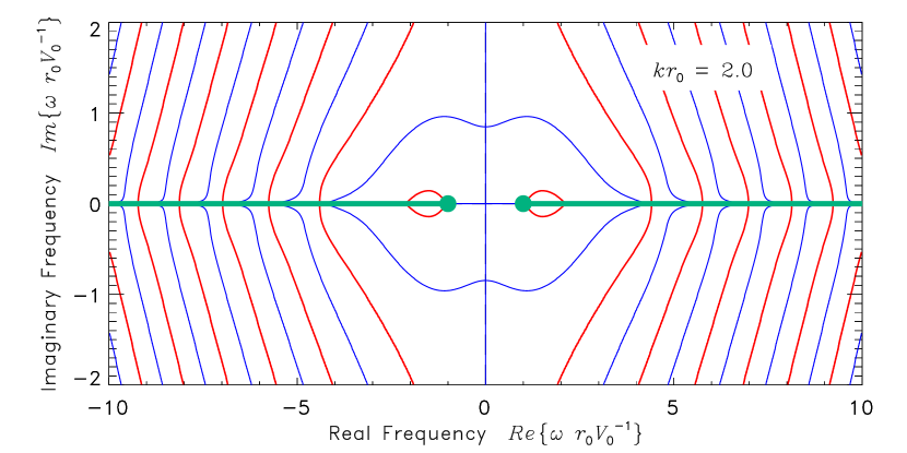
Figure 11: The contours in the complex frequency plane where the real part of the dispersion function $D(k,\omega)$ is zero (red curves) and the imaginary part is zero (blue curves). The wavenumber used in the illustration is purely real, $kr_{0}=2$. The azimuthal order is unity, $m=1$. Wherever a red curve and blue curve cross indicates a complex zero of the dispersion function, and hence the location of an eigenmode. Notice, that no such crossings occur. The teal lines mark branch cuts, locations where the dispersion function is discontinuous. The teal dots indicate the branch points at $\omega=\pm mV_{0}r_{0}^{-1}$. These branch cuts are associated with the continuous spectrum of allowed Alfvén waves. The picture illustrates the dispersion function on only the principle Riemann sheet. The expected fast mode resonances (i.e., zeros of the dispersion function) lie on nearby Riemann sheets that are reached by analytic continuation of the dispersion function through the branch cuts.

In our specific problem, the Alfvén continuum appears as two branch cuts in complex frequency space that lie along the real frequency axis for $\left|\omega\right|>mr_{0}V_{0}^{-1}$. These lines of discontinuity appear because the irregular solution has a logarithmic singularity and hence there are are a countable infinity of potential branches or Riemann sheets. For real frequencies the logarithmic branch point lies on the real radius axis ($r_{\rm A}$ is real). But, if the frequency is complex, the radius of the singularity and branch point is also complex. Further, as the frequency passes across the real axis in the complex frequency plane, the radial branch point also moves across the real radius axis. The inner and outer solutions can be viewed as contour integrals along the real radius axis originating either at the origin or at infinity. Thus, as the radial branch point moves across the integration contour, there is a discontinuity in either the inner or outer solution. A careful consideration of the response of the dispersion function to these discontinuities reveals that there are two branch points on the real frequency axis at $\omega=\pm mV_{0}/r_{0}$ and branch cuts that connect these points to $\pm\infty$ along the real axis. Figure 11 shows contours of the dispersion function $D(k,\omega)$ as a function of complex frequency for a real wavenumber $kr_{0}=2$. The red curves indicate where the real part of the dispersion function is zero and the blue curves are the isocontours where the imaginary part vanishes. The teal dots indicate the two branch points and the teal lines display the branch cuts. Note, nowhere do the red and blue curves cross. Thus, there are no discrete fast eigenmodes that lie on the priniciple Riemann sheet. Thus, the expected set of fast modes are in this case absorbed into the continuous spectrum.

The poles associated with the discrete modes do exist, but they appear on nearby Riemann sheets connected through the branch cuts. It is possible to analytically continue the solutions through the branch cuts to find these poles. Doing so requires that one calculate the inner and outer solutions by integrating off the real radius axis in such a way that the logarithmic singularity never crosses the integration contour. Unfortunately, this requires that the branch cut in radius space crosses the real radius axis for frequencies with a negative imaginary part. Thus, one gains continuity in frequency space at the expense of continuity in radius. Of course for most applications, this is not a useful trade-off.

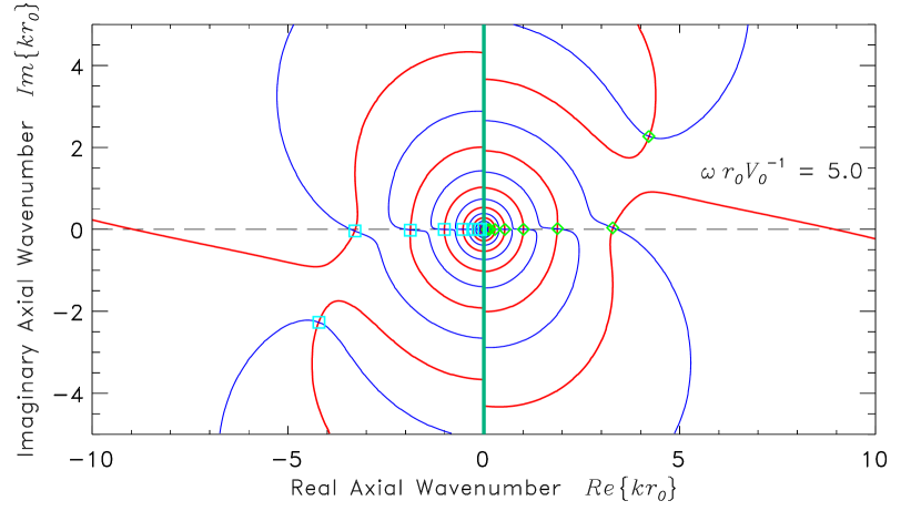
Figure 12: The zero contours of the real part (red) and imaginary part (blue) of the dispersion function in complex wavenumber space. The dispersion function is illustrated for a real dimensionless frequency, $\omega r_{0}V_{0}^{-1}=5.0$ and for a unit azimuthal order, $m=1$. There are many locations where a red curve crosses a blue curve, indicating a fast wave eigenmode of the arcade. There are two families of eigenmodes, those indicated with green diamonds are forward-propagating waves (phase propagates in the positive axial direction), while the aqua squares indicate the symmetric set of counter-propagating waves. There are a countable infinity of each type of mode with an accumulation point at the origin. Only a finite number of modes from each family are indicated in the figure. The imaginary wavenumber axis is a branch cut associated with the behavior of the eigenfunctions at infinite radius. This Riemann sheet, the principle sheet, represents only those solutions which vanish at large radius.

A significantly simpler solution is to invert the spatial transform first and hence consider complex eigenwavenumbers and real frequencies. Since the location of the Alfvén singularity does not depend on the axial wavenumber, the Alfvén continuum does not insert branch points or other singularities in the complex wavenumber plane. Figure 12 illustrates the zero contours of the real and imaginary parts of the dispersion function for a real frequency of $\omega r_{0}V_{0}^{-1}=5$ and for complex wavenumber. There is a branch cut along the imaginary wavenumber axis, but it does not arise from the Alfvén continuum. Instead it corresponds to a continuous spectrum of axially evanescent and radially propagating waves akin to the acoustic jacket modes of helioseismology (see Bogdan & Cally, 1995). Mathematically, this branch cut arises from the behavior of the solution for large radius. In this limit, the solution behaves like a $K$-modified Bessel function, $\Phi\propto K_{\nu}(\sqrt{k^{2}}\,r)$—see Appendix A.2. In order to remain finite at infinite radius, the sign of the square root (i.e., the branch) must change across the imaginary axis, hence, introducing a branch cut. This type of continuous spectrum is well-known and appears in a host of simple problems including the solution in cylindrical coordinates to Poisson’s equation for the electric field generated by a point charge. Note, the red and blue curves cross each other in this case, indicating discrete modes. There are two families of modes, those that propagate in the positive $y$-direction (green diamonds) and those that propagate in the opposite direction (aqua squares). Both families have an accumulation point of modes at the origin (only a finite number of modes have been indicated in the figure). The wavenumbers of the two families are anti-symmetric, with the counter-propagating modes having a wavenumber that is just the negative of the forward-propagating modes. The weakly damped radial overtones ($n>0$) correspond to the countable infinity of poles that lie very near the real wavenumber axis. The strongly damped fundamental mode ($n=0$) appears as two poles (one forward- and one backward-propagating) in a region of complex wavenumber space well away from the real wavenumber axis (near $Im\left\{k\right\}=2.3$). near

Appendix C Energy Flux

The rate at which any given mode loses energy through resonant absorption can be obtained by considering the flux of wave energy. For a magnetically dominated fluid, the energy flux $F$ has two components (Bray & Loughhead, 1974),

$${\mbox{{\boldmath$F$}}}=\left(\frac{{\mbox{{\boldmath$B$}}}\cdot{\mbox{{\boldmath$b$}}}}{4\pi}\right){\mbox{{\boldmath$u$}}}-\frac{{\mbox{{\boldmath$b$}}}\cdot{\mbox{{\boldmath$u$}}}}{4\pi}{\mbox{{\boldmath$B$}}}\;.$$ (C1)

The component of the flux aligned with the background magnetic field arises from the magnetic tension. While this component is in general a nonzero function of azimuth, when integrated over azimuth the term vanishes. This occurs because the transverse components of the perturbed magnetic field $b$ are proportional to $\cos(m\theta)$ whereas the velocity components are proportional to $\sin(m\theta)$—see equations (3.3) and (3.8). Thus, no net energy is lost or gained by fast waves through the action of this flux component. The components of the energy-flux that are transverse to the background field (and result from the magnetic pressure) lack this property.

To ascertain how the energy flux manifests for a single eigenmode, in equation (C1) we must consider only the real parts of the solution and average in time over a wave period. The magnetic pressure fluctuation is directly proportional to $\Phi$—see equation (3.6),

$$\Pi=\frac{{\mbox{{\boldmath$B$}}}\cdot{\mbox{{\boldmath$b$}}}}{4\pi}=\frac{i}{\omega}\,\frac{B^{2}}{4\pi}\Phi\;.$$ (C2)

Therefore denoting the time average by angular brackets, we obtain

$$\left<{\mbox{{\boldmath$F$}}}\right>=\frac{B^{2}}{8\pi\omega}\,Im\left\{\Phi^{*}(r){\mbox{{\boldmath$u$}}}(r)\right\}\,e^{-2\,Im\left\{k\right\}\,y}\,\sin^{2}\left(m\theta\right)\;,$$ (C3)

where we have explicitly included the azimuthal and axial spatial dependences. Note, because of the time averaging (and the real frequencies), the energy flux is independent of time. Further, since the eigenwavenumber is complex, the amplitude of the flux decays in the direction of wave propagation.

The time rate of change of the Alfvén wave energy density is given by the divergence of this energy flux,

$$\frac{\partial{E}}{\partial{t}}=-{\mbox{{\boldmath$\nabla$}}}\cdot\left<{\mbox{{\boldmath$F$}}}\right>$$ (C4)

It can be demonstrated that the divergence of the energy flux vanishes everywhere except at the Alfvén singularity. To do so, apply the chain rule to the product $\Phi^{*}{\mbox{{\boldmath$u$}}}$ and use equations (3.4) and (3.9) to obtain,

$${\mbox{{\boldmath$\nabla$}}}\cdot\left<{\mbox{{\boldmath$F$}}}\right>=\frac{B^{2}}{8\pi\omega}Im\left\{K^{2}\left|{\mbox{{\boldmath$u$}}}(r)\right|^{2}-\left|\Phi(r)\right|^{2}\right\}\,e^{-2\,Im\left\{k\right\}\,y}\,\sin^{2}\left(m\theta\right)=0\;.$$ (C5)

The expression inside the braces is purely real and thus the energy flux is divergenceless.

This is not a surprising result; the waves are ideal MHD waves. The damping of the fast modes occurs purely at the singularity due to a transferral of energy to Alfvén waves. Alfvén waves are not directly described by our ODE (3.11) for a variety of reasons: (1) the Alfvén waves are pure tension waves and thus produce no magnetic-pressure fluctuation, i.e., $\Phi=0$, and (2) the coupled Alfvén waves experience secular growth and therefore do not have exponential time dependence. This latter point can be deduced by carefully examining the rate at which the fast mode pumps energy into the singularity.

As previously stated, the energy flux is divergenceless except at the singularity itself. However, the energy flux can be shown to have a jump discontinuity across the singularity. Hence, the divergence of the flux has a delta function at the singularity. The jump discontinuity arises from the logarithmic singularity in the irregular solution. As shown in Appendix A.3 the irregular solution has the following leading order behavior at the singularity,

$$\Phi_{\rm irr} = 1+\frac{k^{2}}{2}\,(r-r_{\rm A})^{2}\,\ln\left(\frac{r-r_{\rm A}}{r_{0}}\right)+\cdots\;,$$ (C6)

$$u_{{\rm irr},r} = \frac{k^{2}r_{0}^{3}}{\Lambda^{\prime}(0)}\;\ln\left(\frac{r-r_{\rm A}}{r_{0}}\right)+\cdots\;,$$ (C7)

$$\Lambda^{\prime}(0) \equiv r_{0}^{3}\frac{d{}}{d{r}}\left[\frac{\omega^{2}-\omega_{\rm A}^{2}(r)}{V_{\rm A}^{2}(r)}\right]_{r=r_{\rm A}}=-\frac{r_{0}^{3}}{V_{\rm A}^{2}}\left.\frac{d{\omega_{\rm A}^{2}}}{d{r}}\right|_{r=r_{\rm A}}\;.$$ (C8)

Remember that the analytic continuation of the logarithm to negative arguments involves an imaginary component with a Heaviside step function, $H$,

$$\log\left(r-r_{\rm A}\right)=\log\left|r-r_{\rm A}\right|+i\pi H\left(r_{\rm A}-r\right)\;.$$ (C9)

This step function leads to a discontinuous jump in the energy flux across the singularity and energy is continually injected into the singularity. The divergence of the flux has only one term that does not cancel,

$${\mbox{{\boldmath$\nabla$}}}\cdot\left<{\mbox{{\boldmath$F$}}}\right>=\frac{I^{2}\left|A_{\rm irr}\right|^{2}}{2\pi\omega}\,\frac{Re\left\{k^{2}\right\}r_{0}^{3}}{\Lambda^{\prime}(0)}\;Im\left\{\frac{1}{r^{2}}\frac{d{}}{d{r}}\log\left(\frac{r-r_{\rm A}}{r_{0}}\right)\right\}\,e^{-2\,Im\left\{k\right\}\,y}\,\sin^{2}\left(m\theta\right)\;,$$ (C10)

The radial dependence has been made obvious by using equation (2.1) to replace the magnetic field strength with the constant line-current strength, $B=2I/r$. The amplitude of the irregular solution, $A_{\rm irr}$, has units of a frequency and and its amplitude relative to the regular solution, $A_{\rm irr}/A_{\rm reg}$, is fixed by the radial boundary conditions. The energy transfer rate has a delta function for its radial dependence (i.e., arising from the radial derivative of the step function),

$$\frac{\partial{E}}{\partial{t}}=\frac{I^{2}\left|A_{\rm irr}\right|^{2}}{2\omega}\,\frac{Re\left\{k^{2}\right\}r_{0}^{3}}{\Lambda^{\prime}(0)}\;\frac{\delta(r-r_{\rm A})}{r_{\rm A}^{2}}\,e^{-2\,Im\left\{k\right\}\,y}\,\sin^{2}\left(m\theta\right)\;,$$ (C11)

For an Alfvén frequency that is monotonically decreasing with radius (as we have here) the derivative of $\Lambda$ is positive, $\Lambda^{\prime}(0)>0$ (see Figure 1). Thus, the eigensolution injects wave energy into the singularity at a rate that is independent of time.The azimuthally and radially integrated energy in the Alfvén waves grows at a linear rate, $E=E_{0}\left(1+t/\tau\right)$, with $E_{0}$ being the energy at time $t=0$ and $\tau^{-1}$ given by integrating the right-hand side of equation (C11) and divided by $E_{0}$,

$$\tau^{-1}=\frac{\pi I^{2}\left|A_{\rm irr}\right|^{2}}{4\omega E_{0}}\,\frac{Re\left\{k^{2}\right\}r_{0}^{3}}{\Lambda^{\prime}(0)r_{\rm A}}\,e^{-2\,Im\left\{k\right\}\,y}\;.$$ (C12)

This linear growth of the Alfvén wave energy density can be viewed as the root necessity for the Alfvén continuum. The temporal behavior of the Alfvén waves cannot be expressed with a discrete set of exponentials, hence they must be represented as an integral that adds up the contribution of a continuum of exponential forms. This linear combination has the relative phase relations required to build a polynomial in time. This procedure is exactly what continuous spectra from a branch cut often represent.

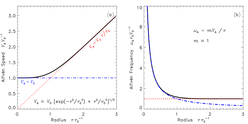
Figure 1: (a) The Alfvén speed, $V_{\rm A}$, given by equation (2.2) shown as a function of cylindrical radius. Near the axis, $r<<r_{0}$, the profile approaches a constant value, $V_{0}$ (shown as the blue dot-dashed line). At large radii, $r>>r_{0}$, the Alfvén speed becomes a linear function of radius (shown as the red dotted line). (b) The Alfvén frequency, $\omega_{\rm A}\equiv mV_{\rm A}/r$, displayed as a function of cylindrical radius for unit azimuthal order, $m=1$. As the radius becomes large the dimensionless Alfvén frequency approaches $m$.

References

- Andries et al. (2009) Andries, J., Van Doorsselaere, T., Roberts, B., Verth, G., Verwichte, E., & Erdélyi, R. 2009, Space Sci. Rev., 149, 3
- Anfinogentov et al. (2013) Anfinogentov, A., Nisticò, G., & Nakariakov, V.M. 2013, A&A, 560, 107
- Appert et al. (1974) Appert, K., Gruber, R., & Vaclivik, J. 1974, Phys. Fluids, 17, 1471
- Arregui et al. (2004) Arregui, I., Oliver, R., & Ballester, J. L. 2004, A&A, 425, 727
- Aschwanden et al. (1999) Aschwanden, M. J., Fletcher, L., Schrijver, C. J., & Alexander, D. 1999, ApJ, 520, 880
- Bogdan & Cally (1995) Bogdan, T. J. & Cally, P. S. 1995, ApJ, 453, 919
- Brady & Arber (2005) Brady, C. S. & Arber, T. D. 2005, A&A, 438, 733
- Bray & Loughhead (1974) Bray, R. J., & Loughhead, R. E. 1974, The Solar Chromosphere (London: Chapman and Hall)
- Chen & Hasegawa (1974a) Chen, L. & Hasegawa, A. 1974a, Phys. Fluids, 17, 1399
- Chen & Hasegawa (1974b) Chen, L. & Hasegawa, A. 1974b, J. Geophys. Res., 79, 1033
- Corless et al. (1996) Corless, R. M., Gonnet, G. H., Hare, D. E. G., Jeffrey, D. J., & Knuth, D. E. 1996, Adv. Comput. Math., 5, 329
- Diáz (2006) Diáz, A. J. 2006, A&A, 456, 737
- Duckenfield et al. (2018) Duckenfield, T., Anfinogentov, S. A., PAscoe, D. J., & Narkariakov, V. M. 2018, ApJ, in press
- Edwin & Roberts (1982) Edwin, P. M. & Roberts, B. 1982, Sol. Phys., 76, 239
- Goddard et al. (2016) Goddard, C. R., Nisticò, G., Nakariakov, V. M., & Zimovets, I. V. 2016, å, 585, A137
- Goedbloed (1971) Goedbloed, J. P. 1971, Physica, 53, 501
- Goedbloed (1975) Goedbloed, J. P. 1975, Phys. Fluids, 18, 1258
- Goedbloed & Poedts (2004) Goedbloed, J.P. & Poedts, S. 2004, Principles of Magnetohydrodynamics, (Cambridge Univ. Press: Cambridge), ISBN 978-0-521-62347-6
- Goosens et al. (1985) Goossens, M., Poedts, S., & Hermans, D. 1985, Sol. Phys., 102, 51
- Goossens et al. (2002) Goossens, M., Andries, J., & Aschwanden, M. J. 2002, A&A, 394, L39
- Goossens et al. (2011) Goossens, M., Erdélyi, R., & Ruderman, M. S. 2011, Space Sci. Rev., 158, 289
- Hain & Lüst (1958) Hain, K. & Lüst, R. 1958, Z. Naturforsch., 13a, 936
- Hindman & Jain (2014) Hindman, B. W. & Jain, R. 2014, ApJ, 784, 103
- Hindman & Jain (2015) Hindman, B. W. & Jain, R. 2015, ApJ, 814, 105
- Hollweg & Yang (1988) Hollweg, J. V. & Yang, G. 1988, J. Geophys. Res., 93, 5423
- Hollweg (1990) Hollweg, J. V. 1990, J. Geophys. Res., 95, 2319
- Kerner et al. (1985) Kerner, W., Lerbinger, K., Gruber, R., & Tsunematsu, T. 1985, Comput. Phys. Commun., 36, 225
- Kerner et al. (1986) Kerner, W., Lerbinger, K., & Riedel, K. 1986, Phys. Fluids, 29, 2975
- Kivelson & Southwood (1985) Kivelson, M. G. & Southwood, D. J. 1985, Geophys. Res. Lett., 12, 49
- Kivelson & Southwood (1986) Kivelson, M. G. & Southwood, D. J. 1986, J. Geophys. Res., 91, 4345
- Lee & Roberts (1986) Lee, M. A. & Roberts, B. 1986, ApJ, 301, 430
- Nakariakov et al. (1999) Nakariakov, V., Ofman, L., DeLuca, E., Roberts, B., & Davila, J. M. 1999, Science, 285, 862
- Nisticò et al. (2013) Nisticò, G., Nakariakov, V.M., & Verwichte, E. 2013, A&A, 552, 57
- Oliver et al. (1998) Oliver, R., Murawski, K., & Ballester, J. L. 1998, A&A, 330, 726
- Pao & Kerner (1985) Pao, Y. P. & Kerner, W. 1985, Phys. Fluids, 28, 287
- Poedts et al. (1985) Poedts, S., Hermans, D., & Goossens, M. 1985, A&A, 151, 16
- Poedts & Goosens (1988) Poedts, S. & Goossens, M. 1988, A&A, 198, 331
- Poedts & Kerner (1991) Poedts, S. & Kerner, W. 1991, Phys. Rev. Lett., 66, 2871
- Rial et al. (2010) Rial, S., Arregui, I., Terradas, J., Oliver, R., & Ballester, J. L. 2010, ApJ, 713, 651
- Rial et al. (2013) Rial, S., Arregui, I., Terradas, J., Oliver, R., & Ballester, J. L. 2013, ApJ, 763, 16
- Ruderman & Roberts (2002) Ruderman, M. S. & Roberts, B. 2002, ApJ, 577, 475
- Selwa et al. (2005) Selwa, M., Murawski, K., Solanki, S. K., Wang, T. J., & Tóth, G. 2005, A&A, 440, 385
- Smith et al. (1997) Smith, J. M., Roberts, B., & Oliver, R. 1997, A&A, 317, 752
- Southwood (1974) Southwood, D. J. 1974, Planet. Space Sci., 12, 483
- Terradas et al. (1999) Terradas, J., Oliver, R., & Ballester, J. L. 1999, ApJ, 517, 488
- Thackray & Jain (2017) Thackray, H. & Jain, R. 2017, A&A, 608, A108
- Uberoi (1972) Uberoi, C. 1972, Phys. Fluids, 15, 1673
- Verwichte et al. (2006a) Verwichte, E., Foullon, C., & Nakariakov, V. M. 2009, A&A, 446, 1139
- Verwichte et al. (2006b) Verwichte, E., Foullon, C., & Nakariakov, V. M. 2009, A&A, 449, 769
- White & Verwichte (2012) White, R. S. & Verwichte, E. 2012, A&A, 537, A49
- Wills-Davey & Thompson (1999) Wills-Davey, M. J. & Thompson, B. J.. 1999, Sol. Phys., 190, 467
- Wright (1992) Wright, A. N. 1992, J. Geophys. Res., 97, 6429