Artificial guide stars for adaptive optics using unmanned aerial vehicles

Abstract

Astronomical adaptive optics systems are used to increase effective telescope resolution. However, they cannot be used to observe the whole sky since one or more natural guide stars of sufficient brightness must be found within the telescope field of view for the AO system to work. Even when laser guide stars are used, natural guide stars are still required to provide a constant position reference. Here, we introduce a technique to overcome this problem by using rotary unmanned aerial vehicles (UAVs) as a platform from which to produce artificial guide stars. We describe the concept, which relies on the UAV being able to measure its precise relative position. We investigate the adaptive optics performance improvements that can be achieved, which in the cases presented here can improve the Strehl ratio by a factor of at least 2 for a 8 m class telescope. We also discuss improvements to this technique, which is relevant to both astronomical and solar adaptive optics systems.

1 Introduction

Unmanned aerial vehicle (UAV) technology has been developing rapidly in recent years, particularly for rotary vehicles (e.g. quadcopters, hexacopters and octocopters). In particular, this has been driven by advances in battery performance, carbon fibre technology, and microcontroller advances. These advances are likely to continue in the foreseeable future, and so here we consider a potential use for UAV technology within astronomy, a field where adoption is relatively new. Biondi et al. (2016) and Chang et al. (2015a) describe UAV based systems that are suitable for calibration of telescopes. Early work by the Pierre Auger Observatory Cosmic Ray Detector took advantage of these advances to characterise the individual pixel sensitivities of their fluorescence telescopes (Bauml, 2013). In particular, an omnidirectional light source was mounted on an octocopter UAV, and positioned 500–1000 m above the telescopes, and individual pixels of these fluorescence telescopes were illuminated. Using the same calibration payload, the sensitivity of other cosmic ray fluorescence detectors were cross-calibrated (Matthews, 2013; Hayashi et al., 2015). Building on this work, the feasibility of using UAVs to calibrate the Cherenkov Telescope Array has also been investigated, including detailed flight characterisation of the UAVs to quantify their contribution to the overall systematic uncertainty of the technique (Brown, 2018; Brown et al., 2016). Other examples of using UAVs to calibrate telescope instrumentation include the characterisation of the far-field beam map of three CROME microwave reflector antennas (Werner, 2013) and the characterisation of the far-field beam map of a single radio dish (Chang et al., 2015b). Fixed wing UAVs have also been proposed as a method of returning astronomical data from a long duration super-pressure balloon airborne telescope, SuperBIT (Romualdez et al., 2016). Here, we explore the potential that this UAV technology has for the field of adaptive optics (AO), including both solar AO and astronomical AO, using UAVs to provide artificial guide stars.

The sky coverage of astronomical AO systems (Babcock, 1953) is limited by the availability of guide stars with sufficient flux close to the astronomical source of interest, even for wide field-of-view Extremely Large Telescope (ELT) instruments (Basden et al., 2014). Even laser guide star (LGS) AO systems (Foy & Labeyrie, 1985) suffer from this since at least one natural guide star (NGS) is required to compensate for the LGS position uncertainty; the true position of the LGS is unknown due to atmospheric turbulence encountered during upward propagation of the laser beam.

For solar AO systems, high spatial resolution observation of the solar limb is difficult, since there are no guide star references with sufficient brightness to be used with a conventional wavefront sensor (Taylor et al., 2015).

Here we present a solution to these problems by introducing a new form of artificial guide star (AGS). For astronomical AO systems, this AGS will provide an absolute position (tip-tilt) signal for a LGS AO system, thereby negating the requirement for NGSs entirely. For solar AO systems, this AGS will provide a high order wavefront sensor target, though without providing low order tip-tilt information. Our proposed techniques use an artificial light source mounted on a UAV platform, as shown schematically in Fig. 1. There are two considerations that are key to this concept. Firstly, the relative position stability of the UAV platform must be sufficient to enable the light source to be maintained within the field of view of a ground-based wavefront sensor (WFS). Secondly, for the astronomical case, the precise relative position of the light source must be known instantaneously, by some means other than optical measurement from the ground.

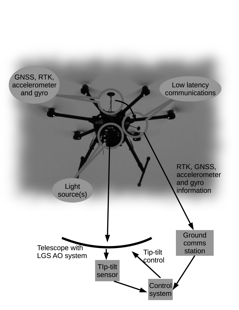
Figure 1: A figure showing the UAV artificial guide star concept: a UAV platform is used to provide support for a light source, low latency communications, and instrumentation with which precise position knowledge can be computed (on the ground). The UAV is observed using a tip-tilt sensor at the telescope, and the raw instrumentation data is sent via a low latency communication link to a ground station. This information is combined with the tip-tilt signal so that actual atmospheric tip-tilt can be computed. Acronym GNSS expands to Global Navigation Satellite System, and RTK expands to Real-Time Kinematic.

The concept that we are proposing will become increasingly feasible as UAV performance increases. Therefore we are attempting to outline a potential future technology for AO, rather than being restricted by currently available UAV models. For example, recent developments with hydrogen fuel cells has led to bespoke UAVs with significantly increased flight times and maximum altitudes.

1.1 Tip-tilt correction for astronomical AO

The concept that we introduce here sees the UAV hovering at a significant altitude (e.g. 1 km or more) above a ground-based telescope, situated along its current line of sight, tracking the telescope motion. The necessary information to compute the precise relative instantaneous position of the UAV (accelerometer, Real-time Kinematic (RTK) and gyroscope measurements) will be relayed to the ground using a low latency wireless communication link, and the relative position of a light source mounted on the UAV as seen by the telescope will be measured by either a tip-tilt wavefront sensor, e.g. a single sub-aperture Shack-Hartmann WFS (for the astronomical case), or a high order wavefront sensor (for the solar case, and possibly the astronomical case). By combining this optical position measurement with the UAV derived instantaneous position estimation, the incident wavefront tilt can be estimated and hence corrected using an active mirror component, for example a deformable mirror (DM).

At good observatory sites typical astronomical seeing is around 0.7 arcseconds. Any tip-tilt correction must lead to an improvement over natural seeing. In this paper, we consider a goal of 0.1 arcsecond precision in tip-tilt correction as a baseline, though we note that this is not an intrinsic limitation of the method described here, but one which would give a definite image quality improvement. For an object (i.e. the UAV) placed at 1 km from a telescope, a 0.1 arcsecond resolution corresponds to a lateral displacement of about 0.5 mm. At least 1 km altitude is necessary for the UAV in order for it to be (a) in the telescope’s far-field limit and (b) above most of the atmospheric turbulence. Our baseline performance therefore requires a relative instantaneous lateral position knowledge of better than 1 mm for a UAV at greater than 1 km distance. We note that as UAV height increases, a less stringent position knowledge is required to meet the same angular accuracy, or alternatively, better tip-tilt estimation can be obtained. In §2.1, we discuss how instantaneous relative UAV positional information can be obtained. We note that the far-field approximation may not be valid if the UAV it stationed close to turbulent layers, and we investigate different propagation models in §3.2.4. However, to avoid this problem, the UAV can be operated at heights that do not correspond to turbulent layers.

Depending on UAV flight stability, it may not be possible to maintain the UAV source position within the WFS field of view. In this case, an array of light sources can be used to ensure that at least one is within the WFS field of view (typically 2–10 arcseconds), with the source closest to the centre of the field then being identified and used by the AO system. These sources can be tracked in the AO system software so that which source is currently within the field of view is known, and when switching between sources (i.e. when the UAV position has changed significantly), the relevant slope offset corresponding to the known change in source position can be subtracted from the wavefront slope measurement. It should be noted that operation of an AGS at low altitudes will mean that only low level turbulence tip-tilt can be measured. We discuss this in section §2.3. A key feature of a UAV AGS is the ability to rapidly reach the desired sky position. For current UAV technology a 1 km altitude can be reached in 2–5 minutes, depending on payload, telescope zenith angle and UAV model.

1.2 Wavefront measurement for solar AO

For solar limb studies using solar AO systems, a high order wavefront sensor reference is required. The UAV will therefore track the solar motion at a distance from the telescope of at least 1 km, maintaining a position along the line of sight to the solar limb. For morning or evening observations, when the sun is low in the sky, this distance could be significantly larger, with the UAV launched some distance from the telescope. We note, of course, that this would not be an attractive option at solar observatories on isolated mountain tops (e.g. Hawaii or La Palma), since a UAV launched far from the observatory would then have to climb a significant height just to reach the observatory altitude. As long as the UAV source position is maintained within the wavefront sensor field of view, and within an isoplanatic patch size (typically 1-10 arcseconds depending on conditions and observation wavelength), the UAV position (from which tip-tilt information is derived) is unimportant, since faint solar structures can be used to obtain the tip-tilt signal, using the whole telescope aperture. Instead, high order wavefront information will be obtained, and used to reconstruct the high order wavefront. The tip-tilt (position) information from the UAV will be discarded, being instead retrieved from a global image of the limb structure. Additionally, in the case where science image acquisition is fast enough (as can sometimes be the case for solar AO), lucky imaging techniques (Law et al., 2006; Basden, 2014b) can be used to shift the images thereby removing the tip-tilt errors.

The wavefront sensor will view a light source on the UAV and this information will be used to reconstruct the incident wavefront. The tip-tilt information will be discarded. We note that this is contrary to the astronomical case, where only the low order information is required. Hence, the solar implementation will be technologically less demanding, since precise position knowledge is not necessary. Fig. 2 demonstrates this concept, and it should be noted that when lower in the sky, the UAV can be launched further from the telescope, thus reducing focal anisoplanatism, assuming some constant maximum altitude can be reached by the UAV. Although the sun is bright, a narrow bandwidth light source can be used so that the UAV signal is above that of the solar background.

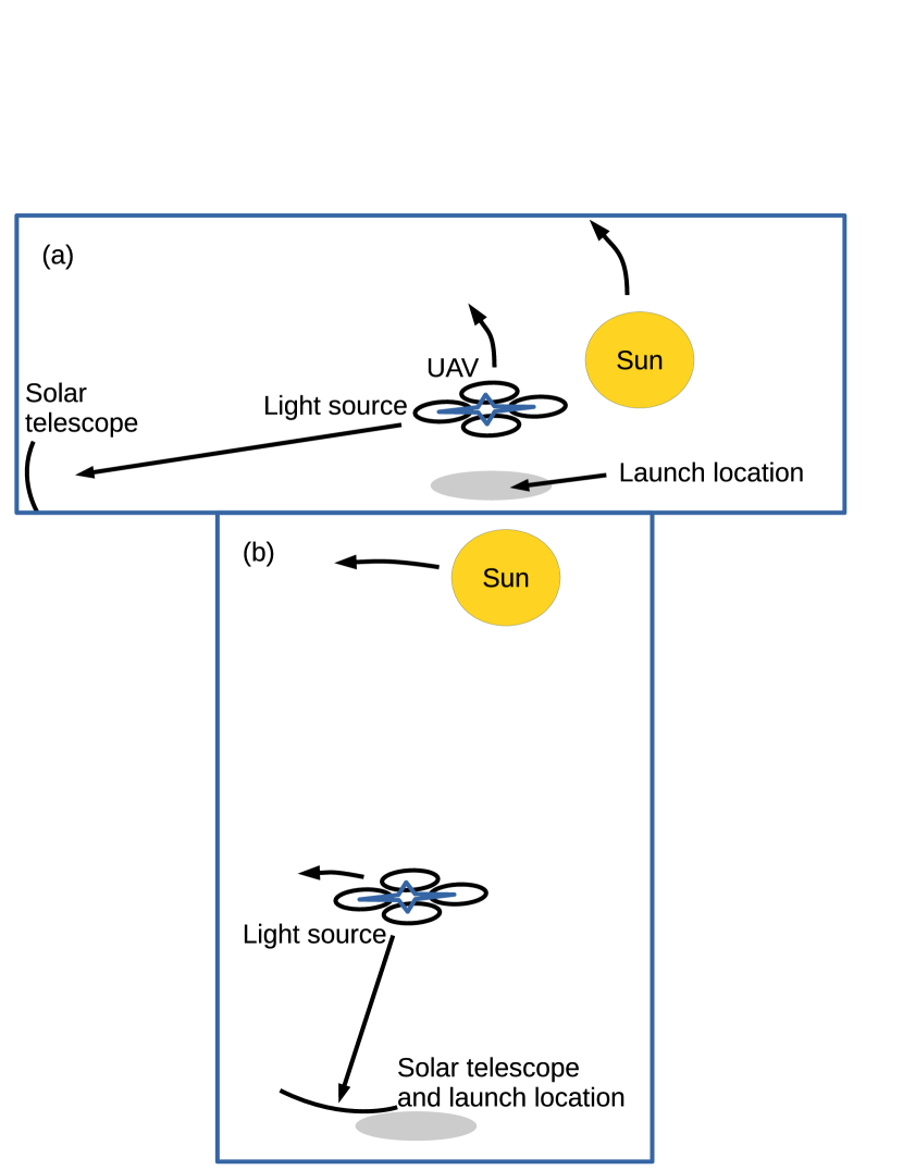
Figure 2: A figure showing the solar UAV technique. The UAV tracks the solar motion as seen by the telescope, and the light source is viewed by a wavefront sensor at the telescope, allowing high order wavefront information to be retrieved. The distance to the UAV can be greater when the sun is lower in the sky, due to the reduced altitude that the UAV has to reach. (a) shows the case when the sun is low, with the UAV launched far (e.g. several km) from the telescope. (b) shows the case when the sun is higher in the sky, with the UAV launched from close to the telescope.

1.3 Overview of current rotary UAV technology

In recent years, the popularity of rotary UAV technology (which we hereafter refer to as simply UAV technology since fixed wing systems are not appropriate for this application) has grown rapidly, driven by the consumer market, in particular the photographic and cinematics industries. Many commercial applications have also become feasible, including within agriculture, the film industry, search and rescue, sports, and infrastructure inspection. This has led to rapid improvements in UAV technology and capability.

Table 1 provides a performance summary for a number of current commercially available systems. With some exceptions, flight time is typically limited to 40 minutes, and payloads of up to 10 kg. We note that in these cases, flight time relates to that achievable by a UAV equipped with standard equipment (battery capacity, propeller type), and therefore should be seen as a minimum achievable. Advances in battery technology means that flight times are likely to extend to one hour for high-end systems within the next few years. The use of hydrogen fuel cells has been shown to extend flight times beyond two hours, and commercial options are becoming more readily available. It should also be noted that UAVs have flown at Mount Everest base camp, at an altitude of about 5,300 m, showing that the thinner atmosphere at these heights does not preclude UAV flight. Optimisation of propeller designs can also further improve performance at higher altitudes.

Model	Type	Payload	Flight time
Yuneec Tornado	Hexa	2 kg	24 min
DJI Matrice 600	Hexa	6 kg	38 min
DJI Agras	Hexa	10 kg	24 min
DJI S1000	Octo	5 kg	15 min
Multirotor Eagle	Octo	2.5 kg	20 min
Multirotor Skycrane	Octo	6.5 kg	12 min
Firefly	Hexa	6.8 kg	15 min
Quarternium Hybrix 2	Quad	2kg	120 min
(petrol)
HyDrone 1550	Hexa	5kg	150 min
(hydrogen fuel cell)

Table 1: A performance summary for a number of commercial UAV systems. Flight times are when hovering, and would not include ascent and descent times. Current UAVs can ascend to 1 km in 2–5 minutes, depending on payload and model, while descent times are usually slightly longer due to downdraught effects, i.e. the UAV descending into the turbulence that it has created.

We present techniques to obtain instantaneous relative UAV position and some conceptual designs for these AGS systems in §2, along with preliminary investigations that we have performed in §3, including Monte-Carlo AO system modelling. Our conclusions are formed in §4.

2 Artificial guide stars using a UAV platform

The concept that we describe here has several key requirements. The UAV would be required to maintain its position for the duration of a science observation, or the ability to pause science integration while UAVs are changed. The UAV must be able to maintain a knowledge of its relative lateral position to high precision (of order 1 mm). Its altitude must also be known, though with a somewhat relaxed precision, such that measurement from the ground is sufficient. The UAV must be able to follow a pre-programmed flight path, and accept minor adjustments to position while in flight. The UAV must also carry a payload with light sources, position sensors, and a low latency communication link to the ground station, with sufficient bandwidth to transfer sensor information (MBit/s) with a latency of 1 ms or lower (below the atmospheric coherence time).

In this section, we discuss requirements and identify techniques that can be used to improve AO capability using the AGS concept.

2.1 UAV-determined position

There are a number of techniques that have the potential to determine UAV instantaneous relative position with the required accuracy. For improved accuracy these techniques could be used in combination. Lateral position is key for this application, however most of these techniques will also be able to determine vertical position with greater precision than is required.

2.1.1 Real-time kinematics

The use of RTK information (Gurusinghe et al., 2002) is a standard approach by which position relative to a base station can be measured with typical accuracy of order one centimetre, though accuracy decreases with distance from the base station. The RTK technique works by using the phase of global navigation satellite systems (GNSS) carrier signals and the base-station link, rather than just the content of these signals. Although this precision is not sufficient to meet the requirements here (approximately 1 mm), future improvements are possible, and it can serve as a baseline measurement since it provides position relative to a fixed ground station.

2.1.2 Accelerometer and gyroscope measurements

Accelerometer measurements can be integrated (twice) to obtain position information (given an initial starting position and velocity). By using a 3-axis accelerometer combined with gyroscopic measurements (to ensure that the correct Cartesian reference frame is used during integration, and to aid gravity subtraction), a 3-d position vector can be obtained (relative to an initial position). Unfortunately, these measurements will contain noise, which when integrated will lead to large position errors rapidly building up, as discussed in §3.1. We therefore propose a solution by which the short-time-period position is obtained using accelerometer and gyroscope measurements, while the long-time-period position is obtained using some other absolute position technique, for example RTK measurements. These measurements can be combined in an optimal way using a Kalman filter (Kalman, 1960; Crassidis, 2006). This is very similar to the SuperBIT telescope pointing system described by Romualdez et al. (2016), where guide star measurements are read out slowly and high frequency gyroscopic data are integrated in between. However, in this case, a Kalman filter is not explicitly used.

The Kalman filter is designed to combine information in the presence of uncertainty, namely the errors associated with accelerometer and RTK sensor information. The uncertainties in absolute position (from the RTK sensor) will be relatively large (of order 1 cm), while accelerometer uncertainty will be much smaller. Fortunately, this concept does not rely on an absolute position, but rather, a position measurement relative to some starting point. Combining the change in position derived from accelerometer measurements (which update rapidly within millisecond timescales) with the direct measurements from the RTK (updating at a few Hz) using a Kalman filter will therefore provide a far more accurate relative position knowledge than using only one of these sensors alone.

2.1.3 Ground base stations

An alternative technique to estimate relative instantaneous UAV position is the use of multiple ground base stations to receive a microwave pulse or amplitude modulated continuous coherent signal from the UAV. The pulse time of arrival, or phase of a continuous signal at these receiver stations can then be used to triangulate the UAV position, relative to a calibrated intial location. Atmospheric effects will lead to uncertainty in these measurements. However, given a sufficient number of receivers, and by operating the UAV at a height away from significant turbulence, we anticipate that these uncertainties can be largely mitigated, leading to a sufficiently accurate position estimation. Fig. 3 illustrates this technique.

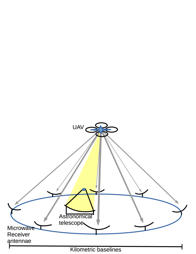
Figure 3: A figure demonstrating the use of multiple ground base stations to triangulate relative UAV position, using time of arrival measurements of a pulse emitted by the UAV. The phase of a continuous signal could also be used. In this figure, the grey arrows represent the microwave pulses, while the yellow beam is the AGS signal. Microwave receiver telescopes are spread over a large area to improve triangulation accuracy.

The microwave pulse can be produced using a Rapid Automatic Cascode Exchange (RACE) generator (Libove et al., 2008), giving a well defined pulse shape and time. Femto-second level timing accuracy will be required to measure pulse arrival times with 1 mm positional accuracy.

Since the complexity of these triangulation approaches is high, requiring multiple ground stations and high precision timing, it will not be cost effective compared with the on-board sensor approach outlined previously. We therefore do not consider it further here.

2.1.4 Optical measurements

We note here that the use of direct optical measurements to determine UAV position, e.g. processing of images of the ground taken by the UAV, does not provide a position estimation with sufficient accuracy since these measurements will be affected by the atmospheric turbulence that is to be corrected. However, rotational information can be obtained by direct optical measurement, supplementing gyroscopic measurements. A camera on-board the UAV, facing the ground (or at night time, the sky), can be used to estimate the instantaneous pitch, roll and yaw of the UAV, by correlating image frames with a reference.

By combining the use of RTK, accelerometer and gyroscope information with imaging, and triangulation using multiple ground base stations, improved position estimates can be obtained. However, for simplicity, we do not consider this further here, rather concentrating on the accelerometer based approach.

2.2 Multiple guide stars for tomographic tip-tilt determination

The AGS technique described here does not allow the full volume of atmospheric turbulence to be probed, since the UAV is not at an infinite distance from the telescope, as shown in Fig. 4. This therefore results an a rather extreme “cone effect”, or focal anisoplanatism (Tallon & Foy, 1990). This is less pronounced in the solar AO case when observing at low zenith angles (morning or evening) since the UAV can be further from the telescope, i.e. it can be launched from a more suitable location (Fig. 2).

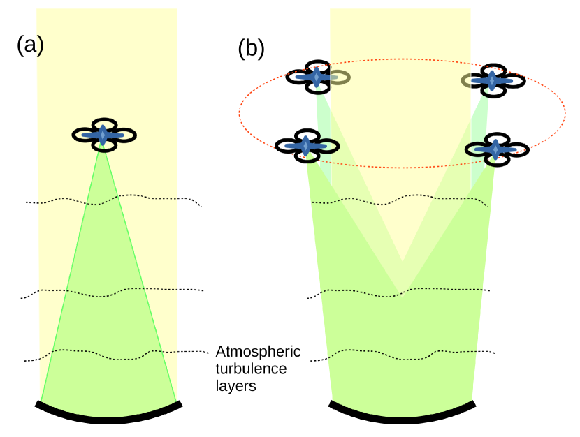
Figure 4: (a) Showing focal anisoplanatism due to the finite altitude of the UAV AGS light source. (b) Mitigation of focal anisoplanatism using multiple AGS, which allow a larger volume of turbulence to be sampled. Only turbulence within the green area will be measured by the wavefront sensor.

A partial solution to this focal anisoplanatism is to use multiple AGS and compute a tomographic wavefront reconstruction of the turbulence (Ellerbroek, 2004; Ellerbroek & Rigaut, 2000; Rigaut, 2002; Beckers, 2002; Tokovinin et al., 2001; Ragazzoni et al., 1999; Morris et al., 2013). This will allow the identification of turbulent wavefronts as a function of height across a wider field of view, and therefore projection along the telescope line of sight to obtain the integrated wavefront in this direction. The tip-tilt information can be obtained with greater accuracy, and in particular, the tip-tilt signal introduced by the strong atmospheric ground layer can be isolated.

For solar AO, where high order wavefront sensor information is required, the use of multiple AGS will yield improved AO performance, due to the reduction in focal anisoplanatism, and in particular, improved determination of wavefront perturbations introduced by the typically strong ground layer.

2.3 Turbulence above the UAV

Since the AGS is at a finite altitude within the Earth’s atmosphere, there will usually be atmospheric turbulence above the UAV, which will then be unsensed by the wavefront sensor. This will therefore degrade the AO system performance. This can be somewhat mitigated by operating the UAV at a higher altitude, though physical restrictions (limited flight times, ability to operate in the thinner atmosphere) currently mean that the UAV cannot reach an arbitrary height.

Fortunately, at many astronomical sites, e.g. the Roque de los Muchachos on La Palma, ground layer turbulence is responsible for the majority of introduced wavefront phase perturbations.

During day time observations, Townson et al. (2015) find that the vast majority of turbulence is at the ground, as high as 95% in some cases.

During night time observations, using the CANARY instrument on the William Herschel Telescope at the Roque de los Muchachos observatory on La Palma, Martin et al. (2017) find that median seeing of the ground layer (up to 1 km) is 0.59 arcsec, while the combined seeing of higher altitudes is 0.21 arcsec with a standard deviation of 0.09 arcsec.

Likewise, García-Lorenzo & Fuensalida (2011a) find that between 67-76% of turbulence during median conditions is situated in the boundary layer, with more than 95% of this below 500 m, at this site.

At the Cerro Paranal site, Masciadri et al. (2012) find that for median conditions, the atmosphere below 1 km contributes to a seeing of 0.9 arcsec, while above this introduces about 0.45 arcsec.

At Teide observatory, García-Lorenzo & Fuensalida (2011b) find that 60% of turbulence is within the boundary layer (up to 1 km) for the average profile, increasing to 72% for the median profile, with 85% of optical turbulence in the lower layers (below 5 km).

On Mauna Kea, Tokovinin et al. (2005) find that optical turbulence in the first 700 m above ground contribute to typically half of the total integrated seeing.

It should also be noted that these seeing estimates generally do not include dome seeing, which can be a large contribution to observed seeing at a telescope (though varies depending on dome structure, site and wind direction). Therefore, the ground layer turbulence as seen by an AO system will usually constitute a greater fraction of overall turbulence than is reported from external seeing monitors. Therefore, significant improvement in optical quality will be possible by just correcting for these ground layers. For the astronomical case, only higher layer tip-tilt would remain uncorrected. For the solar case, higher order information above the UAV height would remain uncorrected.

2.4 Optical leverage of turbulence close to the UAV

If the UAV light source is located close to a turbulent layer, then the patch of this turbulence viewed by the telescope will be small due to focal anisoplanatism. A small tilted region of phase can therefore impart a larger shift in observed source position (Ragazzoni et al., 1997). However, by operating the UAV at heights away from strong turbulence layers, this effect can be largely mitigated, particularly for smaller telescopes. Increasing the altitude of the UAV also reduces the strength of this effect, as focal anisoplanatism is less severe. The simulations which we present in §3 implicitly include this effect.

2.4.1 UAV signals combined with LGS uplink tomography

It has been shown that for tomographic AO systems, some LGS tip-tilt information can be obtained for higher layer turbulence (Reeves, 2015). Therefore, by combining this information with tomographic UAV tip-tilt information (which includes lower layer atmospheric tip-tilt information), improved tip-tilt information can be retrieved, and hence AO correction improved.

2.5 Science field obscuration

Placing a UAV within a telescope’s field of view has the potential to block light and obstruct the point spread functions of the science images. Downdraught produced by the UAV may also introduce some wavefront perturbations. However this can largely be mitigated by operating the UAV at an altitude away from inversion layers, i.e. where the atmosphere is at a constant temperature. In this case, although the downdraught will be turbulent, changes in refractive index (caused by temperature changes) will largely not be present. The typical turbulent cell size produced by a UAV, and dynamics of these, is currently under investigation. Additionally, if the UAV is kept downwind of the telescope, any UAV-produced turbulence will not be seen in the science image. Unlike a laser guide star, a waveband filter cannot be used because the UAV is physically present at the guide star location, i.e. the UAV will block some light to the science detector, and modify the instrumental point spread function (PSF). This will obviously have an impact on the astronomical science, and therefore should be minimised for science cases where accurate PSF shape is important.

There are several possible solutions. First is the possibility of stationing the UAV behind the telescope central obscuration. Since the wavefront sensor for the AGS is not focused at infinity, it will therefore see the UAV, while the science path will not be affected. This is particularly appropriate for larger telescopes, where the central obscuration is larger, as shown in Fig. 5. We note that as the telescope field of view or UAV height increases, the area over which the UAV can remain hidden decreases for a non-zero science field of view.

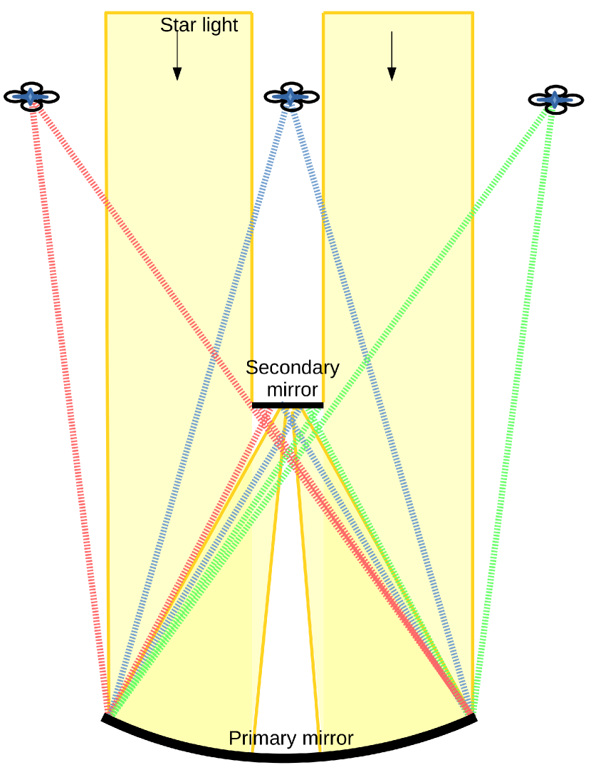
Figure 5: A figure showing UAV locations that would not interfere with science measurements, behind the central obscuration (with the AGS light path shown in blue), or beyond the field of view (with the AGS light path shown in green and red). Star light is represented by the column of yellow, coming from a source at infinity.

The second possibility is to station multiple UAVs outside the telescope scientific field of view, and perform a tomographic wavefront reconstruction. This introduces additional complexity, but has the advantage that the focal anisoplanatism can be mitigated (as discussed previously), and performance across the field of view increased.

In both of these cases, care must be taken to ensure that the UAV does not drift into the science field (e.g. due to a gust of wind). It is possible that mitigation steps can be taken, i.e. if the UAV moves too far from its expected position, the light source could be turned off to avoid polluting science images (though this would result in the loss of tip-tilt information, particularly if only one UAV is in use), or a narrow band filter could be used on the science path to block the UAV signal (though obscuration would still occur).

Stray light from the UAV source due to multiple Rayleigh scattering may also be present, and so it may be desirable to have a narrow band filter present to stop this. However, if the UAV is faint this is unlikely to be a problem: since the UAV used for a tip-tilt signal only (not higher orders) on a large telescope aperture, a signal of 15–16 th Magnitude may be usable, and therefore Rayleigh scattering will be negligible.

For an 8 m telescope with a UAV at 1 km at the edge of the on-axis science field (i.e. the cylindrical observation beam) the UAV would appear about 13 arcmin off axis. This is a large field of view for an astronomical AO system, and it is highly likely that a suitable NGS could be found within this field, particularly within the galactic plane, meaning that sky coverage would approach 100%: the UAV would not be necessary. However, for a UAV at 4 km, this field narrows to 3.5 arcmin, and at 10 km, to 1.4 arcmin, at which point, NGS sky coverage becomes more severely restricted, particularly outside the galactic plane. For a 4 m telescope, a 10 km UAV could be placed about 40 arcsec off-axis without obscuring the on-axis science field. Therefore, the higher the UAV can operate, the larger the gain in achievable sky coverage, though this does not affect an on-axis UAV behind the telescope central obscuration. Here, we have considered only the geometrical shadow of the UAV in the optical beam, rather than the Fresnel effect. However, if the light source was suspended at the side of the UAV, rather than centrally mounted, the Fresnel effect would be small.

2.6 UAV flight time limitations

Flight time of current UAVs is currently restricted to less than one hour by limitations in battery technology. Hydrogen fuel cell developments have shown that flight time can be increased to more than 2 hours. However, even though battery and fuel cell technology is rapidly improving, short flight times will still be the reality (compared with night-long science observations), particularly since time required to reach altitude and return safely must be included. This can therefore be problematic when long astronomical science exposures are required, and there are two possible solutions that we have identified.

2.6.1 In-observation swapping of UAVs

The first solution is to perform in-flight swapping of UAVs, such that a fully charged replacement is scheduled to take the position of a UAV that needs to return for recharging. During this operation, the new UAV would manoeuvre to the required altitude, just beyond the telescope field of view. This operation would occur in between science integrations, which are typically split into individual exposure of not more than 30 minutes each. The AO loop would be disengaged, and the UAVs would swap position. The new UAV would then be acquired by the wavefront sensor and the AO loop engaged, and once stabilised, the next science exposure started. With full automation, this procedure could be expected to have negligible impact on most science observations, and would be expected to result in less than one minute of down-time.

2.6.2 In flight recharging

A second solution for limited flight time is to develop in-flight recharging capabilities, based on wireless energy transmission (Angrisani et al., 2015). This has previously been demonstrated with a helicopter using microwave energy transfer (Brown, 1965). This would require a ground-based high power microwave transmitter, which would send a directed beam to a receiver on the UAV, where the energy would be collected and stored. We note however that we have not investigated the practicality of this scheme.

2.7 Autonomous operation

The UAV application proposed here would operate autonomously, to remove the possibility of pilot error. A fully automated system would enable the UAVs to depart from the base station, manoeuvre to the correct position on-sky ahead of telescope acquisition, and then automatically follow the course of the position change due to telescope tracking. Position offsets derived from the wavefront sensor signals by the AO system can be sent to the UAV to perform a slow guiding offload.

At the end of operation, the UAV would return to the base station, and automatically begin recharging. Therefore once such a system has been commissioned, minimal operator intervention would be required beyond routine maintenance.

2.8 In-flight safety

2.8.1 UAV component failure risk

The largest contribution to risk associated with UAV operation comes from pilot error, which is largely mitigated by having a fully autonomous system. However, the introduction of redundancy and fail-safe operation should also be considered. Should a UAV component fail during operation (e.g. a motor), it must be possible for the UAV to return safely to the ground. For this reason, we recommend the use of hexa and octocopters, which are able to fly and land safely in the event of motor failure.

Communication failure is also a possibility, in which case, the UAV should be programmed to return automatically to its launch location, based on a GNSS signal.

Battery failure should be considered, and an auxiliary power supply included.

2.8.2 Collision risk

The risk of a collision of a UAV with the telescope should be considered. However, since telescopes do not usually operate at zenith, a failed UAV is unlikely to fall onto the telescope, though other telescopes on-site might be affected. The UAV would be expected to carry a parachute and a fail-safe mechanism to stop the rotors, to lessen impact velocity and reduce collateral damage to people, other buildings and infrastructure (and the UAV itself).

When multiple UAVs are in operation, there is the risk of in-flight collision. However, this will be largely mitigated by having all flight under computer control, with algorithms to explicitly avoid this scenario, in addition to onboard proximity sensors. Collisions with other aircraft is also possible. The airspace above some observatories is a designated no-fly zone, and therefore these observatories could operate a UAV without collision risk. At other observatories, aircraft spotter systems would be required, as is already the case for LGS systems. A mode S transponder would be carried by all UAVs so that they are uniquely identifiable. The UAVs would also carry proximity sensors to aid collision avoidance with rogue UAV operators. If a collision with a larger aircraft was predicted, it would be the responsibility of the UAV to take avoidance action. Collisions with birds should also be considered.

3 Modelling investigations

Key to the success of this UAV-aided AO technique is the ability to derive the instantaneous relative position from accelerometer measurements. Unfortunately, the double integral required to obtain the position from acceleration data can lead to a rapid (1.5 power) build up of error. We therefore investigate the necessary accelerometer specification required to meet the position knowledge accuracy. Here, we consider only accelerometer measurements, and do not consider the integration with absolute position estimates (RTK), since it has previously been shown that a Kalman filter can be used to optimally combine these measurements. Rather, we concentrate on determining the accelerometer specifications (polling rate and uncertainty) that would be required to meet position estimates for a given period of time.

3.1 Accelerometer position accuracy

We have investigated the accelerometer parameters needed to maintain a position knowledge to within a specified error over a specified time period. In our modelling we include a random thermal (Gaussian) noise uncertainty on the accelerometer output, and also the effect of digitisation of the accelerometer signal. For simplicity, we consider a one dimensional system, and include cases where the accelerometer is at rest, moving with a sinusoidal motion, and undergoing constant acceleration.

3.1.1 Accelerometer at rest or under constant acceleration

We first consider the case of an accelerometer at rest, and input different noise levels into the accelerometer readout process. Using a readout (sampling) rate of 100 Hz (time period of 10 ms), we measure the accelerometer-predicted position over 100 s. We repeat the measurements 100 times.

Fig. 6 shows how the position error grows as a function of time for different accelerometer noise levels, given in ms^-2. When the noise is low, accelerometer position remains accurate to less than 1 mm for 100 seconds. However, in all cases, the position error grows faster than linearly. Thong et al. (2004) show that position error due to accelerometer uncertainty grows as

$$ERR(t)=\frac{1}{\sqrt{3}}\frac{\sigma}{\sqrt{f}}t^{1.5}$$ (1)

where $t$ is the time, $\sigma$ is the rms accelerometer uncertainty and $f$ is the sampling frequency. We find that our modelling is in good agreement with this.

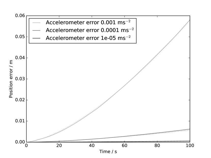
Figure 6: Accelerometer-derived position error as a function of time for different accelerometer noise levels as given in the legend, in ms^-2. Solid curves are Monte-Carlo measurements, while dotted curves show Eq. 1.

Fig. 7 shows how the sampling period affects position error. Here, we use an accelerometer uncertainty of 0.0001 ms^-2 at every sample point. Easily obtainable commercial accelerometers offer sampling rates above 300 Hz, with error (uncertainty) lower than 0.0001 ms^-2 (Beitia et al., 2015). We can therefore see that accelerometer measurements will be able to estimate position with the required accuracy for significant periods of time, beyond which the 1.5 power growth in error can be constrained by RTK measurements using a Kalman filter.

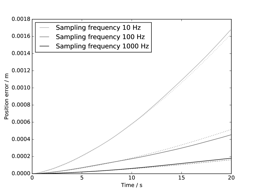
Figure 7: Accelerometer-derived position error as a function of time for different accelerometer sampling rates as given in the legend, in ms^-2. Solid curves are Monte-Carlo measurements, while dotted curves show Eq. 1.

Digitisation (quantisation) of accelerometer signals will occur when the analogue current or voltage generated by the accelerometer is converted to a digital form. If the accelerometer is stationary (or moving with no acceleration), then it can be expected that digitisation of the signal will actually improve performance: if digitisation is taken to the extreme, then all measurements would be exactly zero, and thus, the derived position would also remain zero. This is verified in Fig. 8. However, since the purpose of an accelerometer is to detect changes in motion, study of a static accelerometer is an academic exercise only.

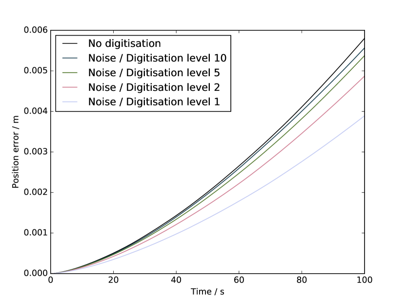
Figure 8: Accelerometer-derived position error as a function of time for different accelerometer digitisation levels as given in the legend, in ms^-2. The value of digitisation given here is the number of times larger than the digitisation level one standard deviation of noise is. Therefore, coarser digitisation is given by a lower number. In this case, sampling rate is 100 Hz, and accelerometer noise is 0.0001 ms^-2.

3.1.2 Accelerometer with sinusoidal motion

Since the UAV will not be stationary, it is important to model an accelerometer-derived position with non-uniform acceleration. To this end, we consider an accelerometer undergoing sinusoidal motion with 10 cm amplitude and 7 s period. This amplitude is chosen as representative (though pessimistic) of UAV stability in conditions of light wind. Accelerometers do not measure instantaneous acceleration, but rather that integrated over a period of time. We therefore include this in our model, using a high resolution time step to generate actual position, while integrating the acceleration over this period. Fig. 9 shows position error as a function of time for a 100 Hz accelerometer sampling rate, with 0.0001 ms^-2 noise. Different digitisation levels are shown, and it is clear here that coarser digitisation gives worse performance. However, the accelerometer-derived relative position estimate is accurate to within 1 mm for about 40 s, which again, is sufficient.

Figure 9: Accelerometer-derived position error as a function of time for different accelerometer digitisation levels as given in the legend, in ms^-2. The value of digitisation given here is the number of times larger than the digitisation level one standard deviation of noise is. Therefore, coarser digitisation is given by a lower number. In this case, sampling rate is 100 Hz, and accelerometer noise is 0.0001 ms^-2. The accelerometer is undergoing sinusoidal motion with a 10 cm amplitude and 7 s period.

3.2 Monte-carlo modelling of AO performance

To investigate the AO system performance gain that a UAV AGS can deliver, we use the Durham AO simulation platform (DASP) (Basden et al., 2007). This Monte-Carlo modelling software has been widely used for AO system modelling (Jia & Zhang, 2013; Basden et al., 2010; Bitenc et al., 2013; Basden, 2014a; Morris et al., 2010; Basden et al., 2014; Jia et al., 2015; Basden, 2015), and includes an end-to-end model of the atmosphere, telescope and AO system.

3.2.1 Model parameters

We investigate the performance of a laser tomographic AO (LTAO) system on a 8 m telescope, using 4 LGSs. No NGSs are used, and the LGS tip-tilt signal is assumed invalid. We assume a sodium layer centred at 90 km with a 10 km full-width at half-maximum (FWHM), and explore two different LGS asterisms, with diameter of 20 arcsec and 60 arcsec (the 4 LGSs are equally spaced on a circle with this diameter). We use $16\times 16$ sub-apertures for each LGS WFS, and assume the use of low noise electron multiplying CCDs (EMCCDs) and high photon return from the sodium layer. The height of the UAV is investigated, and we use a single sub-aperture Shack-Hartmann sensor for measurement of the UAV tip-tilt signal. Each WFS operates at 589 nm. The DM has $17\times 17$ actuators, controlled using the LGS signals, and a separate tip-tilt mirror is used, controlled using the UAV AGS signal.

We use a standard European Southern Observatory (ESO) 35 layer atmospheric profile (Sarazin et al., 2013), with a Fried’s parameter of 15.7 cm and a 30 m outer scale. The AO system performance is measured on-axis at H-band (1650 nm). We use an AO system update rate of 250 Hz, and integrate for 20 s, by which time the AO corrected PSF is well averaged. A 1.2 m telescope central obscuration is assumed. The AO system loop gain is set to 0.5.

The UAV is modelled as a point source. We first assume perfect position knowledge, and then also model Gaussian uncertainty in the measured position of the UAV with rms position uncertainties of 0.5, 1 and 2 mm. In this case, at each simulation time-step, a Gaussian random variable is added to the AGS tip-tilt measurements with a standard deviation equal to the uncertainty in arcseconds (i.e. approximately the arctangent of the position uncertainty divided by UAV height). We use this position uncertainty to model the imperfect position measurement system on the UAV. We note that assuming a Gaussian distribution for position uncertainty is pessimistic: this error will grow non-linearly with time between RTK measurements, and therefore is not well approximated by a Gaussian distribution.

3.2.2 Modelling results

Fig. 10 shows the increase in H-band Strehl as a function of UAV altitude, along with performance without AO, performance using only LGSs (i.e. no tip-tilt correction), and performance using full LGS and NGS AO (with an on-axis NGS tip-tilt sensor instead of a UAV, assumed to be bright, i.e. negligible noise, with the same pixel scale as the UAV tip-tilt sensor). This clearly shows that the use of a UAV AGS can have a significant AO performance benefit. Increasing UAV altitude is beneficial, but even at 1 km, the improvement in AO performance can be significant if position uncertainty is small, compared to the use of LGSs alone. We see that at high altitudes, when accelerometer error is low, performance levels are significantly better than those without the UAV, though remain slightly short of the LGS and NGS combined case, dominated by focal anisoplanatism.

It is evident, as would be expected, that the uncertainty in the UAV position estimate can have a significant impact on performance. In the particular case that we model here, if UAV position uncertainty is 1 mm, then the UAV must be at an altitude greater than 1 km before AO performance improvement is seen. If the position uncertainty is reduced to 0.5 mm, the UAV can operate at a lower height (above 500 m) to achieve some performance benefit. It should be noted that there is always a benefit in operating the UAV at a greater altitude, regardless of the position uncertainty level. We note that these results will be dependent on atmospheric parameters, and that a higher altitude is always desirable.

(a) (b)

Figure 10: (a) AO system performance (H-band Strehl) as a function of UAV height. The uncertainty in UAV position is given in the legend. A comparison with no AO, LGS-only AO, and full NGS+LGS AO is also shown. The LGS asterism diameter is 20 arcsec. The grey regions show the measurement uncertainty. (b) As for (a), but showing residual wavefront error instead of Strehl ratio.

Fig. 11 compares AO performance with two different LGS asterism diameters, and it is evident that a single UAV AGS is able to improve AO performance in both cases.

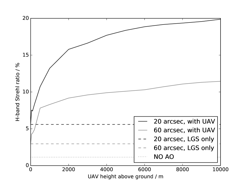
Figure 11: AO system performance (H-band Strehl) as a function of UAV height, for a LGS asterism diameter of 20 and 60 arcsec, as given in the legend. Relative UAV position estimation is assumed to be accurate.

We note that the modelling presented here should not be taken as an absolute performance reference, since this is highly dependent on the atmospheric profile and turbulence strength, which vary from night to night, and from observatory to observatory. Rather, these results should be taken as showing that the concept is valid, and that a UAV AGS can be used to improve LGS-only AO system performance.

3.2.3 Impact of outer scale

Within the literature, there is much debate about the range of values for the atmospheric outer scale. In our modelling we have selected 30 m as the default value. However, we also investigate the AO performance as a function of outer scale from 5–100 m, as shown in Fig. 12. Here, it can be seen that for a UAV at 2 km, performance is always improved, regardless of the outer scale.

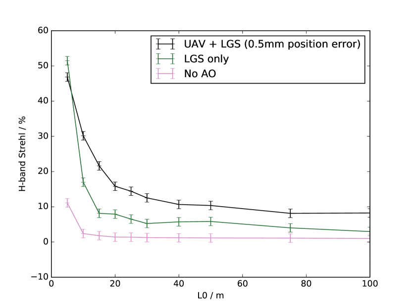
(a) (b)

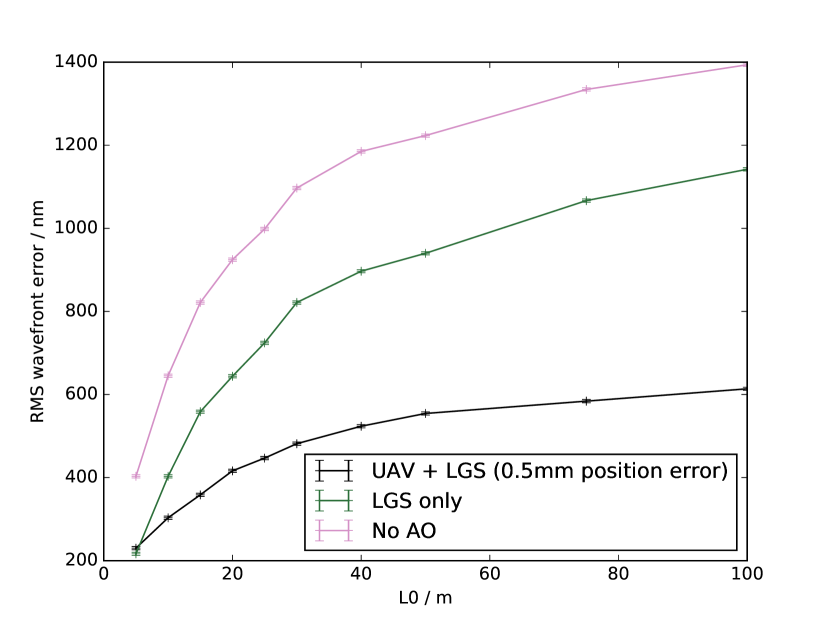
Figure 12: (a) A figure showing AO performance (H-band Strehl) as a function of atmospheric outer scale, for a UAV at 2 km with 0.5 mm position uncertainty for the UAV. (b) As for (a), but showing residual wavefront error instead of Strehl ratio.

3.2.4 Physical propagation models

The Monte-Carlo results presented within this paper use Fourier propagation of the optical wavefront, i.e. converting between far-field (pupil plane) to focal plane. However, we also investigate the use of Fresnel propagation for the AGS source, since this source can be close to the perturbing layers. Fig. 13 shows that the difference between Fresnel and Fourier propagation results is small. At the largest outer scales, Fresnel propagation seems to be slightly pessimistic compared with Fourier propagation, though the difference is typically small (25 nm rms error). We have therefore used Fourier propagation for the rest of this paper, due to reduced computational complexity.

(a)
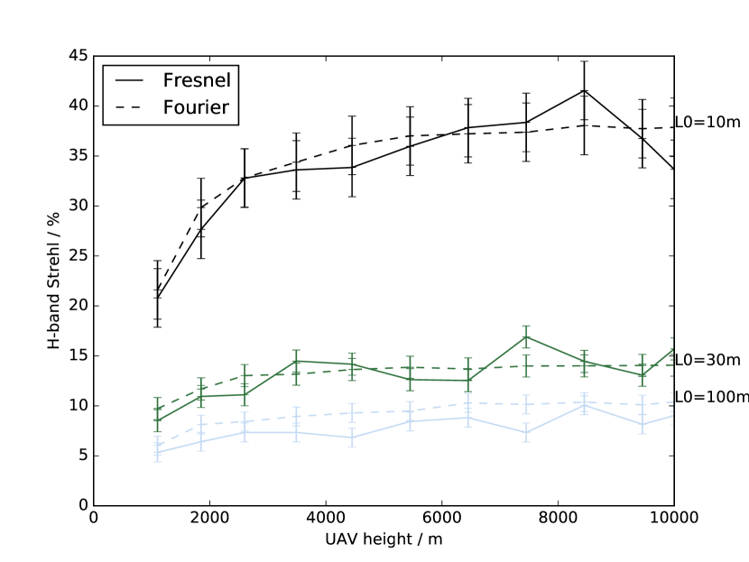
(b)

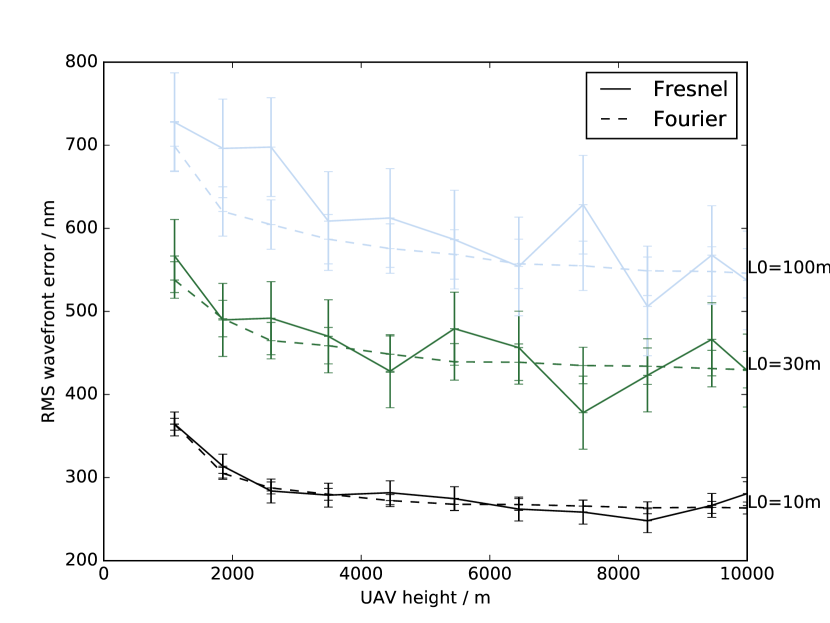
Figure 13: (a) AO system performance (H-band Strehl) as a function of UAV height for different atmospheric outer scale values, using Fresnel propagation models. (b) As for (a), but showing residual wavefront error instead of Strehl ratio.

3.3 Future work

This UAV AGS concept is in its infancy, and therefore much future work is required. Laboratory demonstration of RTK and accelerometer position estimation are under investigation. UAV characterisation is also required, and we are not assuming that the UAV is a ready-made platform, but rather considering how the stability and aerodynamic aspects of the UAV will affect performance. Investigation of UAV turbulence is also being carried out. These investigations will be followed by on-sky testing and verification of this concept, in particular of the ability to provide an AGS reference.

We have also not measured the performance gain achievable with this UAV technique when applied to ELT-scale telescopes. Here, due to the larger telescope diameter, more precise position knowledge is likely to be required for the same gain in Strehl ratio (though other performance metrics such as ensquared energy may perform better): the telescope diffraction limit scales inversely proportional to telescope diameter.

4 Conclusions

We have presented a novel concept using UAVs to provide an AGS signal for adaptive optics systems, allowing full sky coverage to be achieved for AO corrected observations. For astronomical AO, this concept uses a UAV system to provide tip-tilt signals, with higher order correction being performed using LGSs. This enables full sky coverage, as NGSs are no longer required. For solar AO, this concept uses the UAV AGS to provide a high order WFS signal for solar limb observations, where the solar structure itself cannot be used for AO correction. We propose a system using RTK, accelerometers and gyroscopes to provide an accurate instantaneous UAV relative position estimate. Modelling for 8 m class telescopes shows that the UAV should operate in excess of 1 km (with higher altitudes being more favourable), and we note that this is within the range of current UAV technology. We find that Strehl ratio can be increased by a factor greater than two compared to the case of LGS-only AO for the cases studied here. As UAV altitude increases, AO performance improves, and a UAV at 10 km is able to mitigate the vast majority of wavefront tip-tilt, though performance does not quite reach that achieved using a NGS.

References

- Angrisani et al. (2015) Angrisani L., d’Alessandro G., D’Arco M., Paciello V., Pietrosanto A., 2015, in 2015 IEEE International Workshop on Measurements Networking (M N) Autonomous recharge of drones through an induction based power transfer system. pp 1–6
- Babcock (1953) Babcock H. W., 1953, Pub. Astron. Soc. Pacific, 65, 229
- Basden (2014a) Basden A. G., 2014a, MNRAS, 440, 577
- Basden (2014b) Basden A. G., 2014b, MNRAS, 442, 1142
- Basden (2015) Basden A. G., 2015, MNRAS, 453, 3035
- Basden et al. (2007) Basden A. G., Butterley T., Myers R. M., Wilson R. W., 2007, Appl. Optics, 46, 1089
- Basden et al. (2014) Basden A. G., Evans C. J., Morris T. J., 2014, MNRAS, 445, 4008
- Basden et al. (2010) Basden A. G., Myers R., Butterley T., 2010, Appl. Optics, 49, G1
- Bauml (2013) Bauml J., 2013, in Proc. of the 33rd International Cosmic Ray Conference Measurement of the Optical Properties of the Auger Fluorescence Telescopes. pp 806–807
- Beckers (2002) Beckers J., 2002, in Vernin J., Benkhaldoun Z., Muñoz-Tuñón C., eds, Astronomical Site Evaluation in the Visible and Radio Range Vol. 266 of Astronomical Society of the Pacific Conference Series, Multi-conjugate Adaptive Optics: Experiment in Atmospheric Tomography. p. 562
-
Beitia
et al. (2015)
Beitia J., Clifford A., Fell C., Loisel P., 2015, Technical report,
Quartz Pendulous Accelerometers for Navigation and Tactical Grade Systems,
http://www.innalabs.com/download-attachment/872. Innalabs Ltd - Biondi et al. (2016) Biondi F., Magrin D., Ragazzoni R., Farinato J., Greggio D., Dima M., Gullieuszik M., Bergomi M., Carolo E., Marafatto L., Portaluri E., 2016, in Advances in Optical and Mechanical Technologies for Telescopes and Instrumentation II Vol. 9912 of Society of Photo-Optical Instrumentation Engineers (SPIE) Conference Series, Unmanned aerial vehicles in astronomy. p. 991210
- Bitenc et al. (2013) Bitenc U., Rosensteiner R., Bharmal N. A., Basden A. G., Morris T. J., Obereder A., Dipper N. A., Gendron E., Vidal F., Rousset G., Gratadour D., Martin O., Hubert Z., Myers R., 2013, in Proc. Conf. Adaptative Optics for Extremely Large Telescopes 3 Tests of novel wavefront reconstructors on sky with CANARY
- Brown (2018) Brown A. M., 2018, Astroparticle Physics, 97, 69
- Brown et al. (2016) Brown A. M., Chadwick P. M., Frizzelle M., Gaug M., Clark P., Graham J., Armstrong T., 2016, in Ground-based and Airborne Telescopes VI Vol. 9906 of Society of Photo-Optical Instrumentation Engineers (SPIE) Conference Series, Feasibility study of airborne calibration of the Cherenkov Telescope Array. p. 99061W
- Brown (1965) Brown W. C., , 1965, Experimental Airborne Microwave Supported Platform
- Chang et al. (2015a) Chang C., Monstein C., Refregier A., Amara A., Glauser A., Casura S., 2015a, Pub. Astron. Soc. Pacific, 127, 1131
- Chang et al. (2015b) Chang C., Monstein C., Refregier A., Amara A., Glauser A., Casura S., 2015b, Pub. Astron. Soc. Pacific, 127, 1131
- Crassidis (2006) Crassidis J. L., 2006, IEEE Transactions on Aerospace and Electronic Systems, 42, 750
- Ellerbroek & Rigaut (2000) Ellerbroek B., Rigaut F., 2000, Nature, 403, 25
- Ellerbroek (2004) Ellerbroek B. L., 2004, in Ardeberg A. L., Andersen T., eds, Second Backaskog Workshop on Extremely Large Telescopes Vol. 5382 of Society of Photo-Optical Instrumentation Engineers (SPIE) Conference Series, Wavefront reconstruction algorithms and simulation results for multiconjugate adaptive optics on giant telescopes. pp 478–489
- Foy & Labeyrie (1985) Foy R., Labeyrie A., 1985, A&A, 152, L29
- García-Lorenzo & Fuensalida (2011a) García-Lorenzo B., Fuensalida J. J., 2011a, MNRAS, 416, 2123
- García-Lorenzo & Fuensalida (2011b) García-Lorenzo B., Fuensalida J. J., 2011b, MNRAS, 410, 934
- Gurusinghe et al. (2002) Gurusinghe G., Nakatsuji T., Azuta Y., Ranjitkar P., Tanaboriboon Y., 2002, Transportation Research Record: Journal of the Transportation Resear ch Board, 1802, 166
- Hayashi et al. (2015) Hayashi M., Tameda Y., Tsunesada Y., Tomida T., Telescope Array Collaboration 2015, in Borisov A. S., Denisova V. G., Guseva Z. M., Kanevskaya E. A., Kogan M. G., Morozov A. E., Puchkov V. S., Pyatovsky S. E., Shoziyoev G. P., Smirnova M. D., Vargasov A. V., Galkin V. I., Nazarov S. I., Mukhamedshin R. A., eds, 34th International Cosmic Ray Conference (ICRC2015) Vol. 34 of International Cosmic Ray Conference, Calibration of a fluorescence detector using a flying standard light source for the Telescope Array observatory. p. 692
- Jia et al. (2015) Jia P., Cai D., Wang D., Basden A., 2015, MNRAS, 450, 38
- Jia & Zhang (2013) Jia P., Zhang S., 2013, Research in Astronomy and Astrophysics, 13, 875
- Kalman (1960) Kalman R. E., 1960, Boletin de la Sociedad Matematica Mexicana, 5, 102
- Law et al. (2006) Law N. M., Mackay C. D., Baldwin J. E., 2006, A&A, 446, 739
- Libove et al. (2008) Libove J. M., Illingworth B. R., Chacko S. J., 2008, Microwave Journal, 51, 86
- Martin et al. (2017) Martin O. A., Gendron É., Rousset G., Gratadour D., Vidal F., Morris T. J., Basden A. G., Myers R. M., Correia C. M., Henry D., 2017, A&A, 598, A37
- Masciadri et al. (2012) Masciadri E., Lascaux F., Fuensalida J. J., Lombardi G., Vázquez-Ramió H., 2012, MNRAS, 420, 2399
- Matthews (2013) Matthews J. N., 2013, in Proc. of the 33rd International Cosmic Ray Conference Progress Towards a Cross-Calibration of the Auger and Telescope Array Fluorescence Telescopes via an Air-borne Light Source. pp 1218–1225
- Morris et al. (2013) Morris T., Gendron E., Basden A. G., Martin O., Osborn J., Henry D., Hubert Z., Sivo G., 2013, in Proc. Conf. Adaptive Optics for Extremely Large Telescopes 3 Multiple object adaptive optics: Mixed ngs/lgs tomography
- Morris et al. (2010) Morris T., Hubert Z., Myers R., Gendron E., Longmore A., Rousset G., et al 2010, in Adaptative Optics for Extremely Large Telescopes CANARY: The NGS/LGS MOAO demonstrator for EAGLE. p. 08003
- Ragazzoni et al. (1997) Ragazzoni R., Marchetti E., Brusa G., 1997, A&AS, 121, 569
- Ragazzoni et al. (1999) Ragazzoni R., Marchetti E., Rigaut F., 1999, A&A, 342, L53
- Reeves (2015) Reeves A. P., 2015, PhD thesis, Durham University
- Rigaut (2002) Rigaut F., 2002, in Vernet E., Ragazzoni R., Esposito S., Hubin N., eds, European Southern Observatory Conference and Workshop Proceedings Vol. 58 of European Southern Observatory Conference and Workshop Proceedings, Ground Conjugate Wide Field Adaptive Optics for the ELTs. p. 11
- Romualdez et al. (2016) Romualdez J. L., Benton J. S., Clark P., Damaren C., Eifler T., Fraisse A., Galloway N. M. ., Hartley W. J., Jones W., Li L., Lipton L., Luu . V., Massey R. J., Netterfield C. B., Padilla I., Rhodes J., Schmoll J., 2016, J. Aerospace Eng.
- Sarazin et al. (2013) Sarazin M., Le Louarn M., Ascenso J., Lombardi G., Navarrete J., 2013, in Esposito S., Fini L., eds, Proceedings of the Third AO4ELT Conference Defining reference turbulence profiles for E-ELT AO performance simulations. p. 89
- Tallon & Foy (1990) Tallon M., Foy R., 1990, A&A, 235, 549
- Taylor et al. (2015) Taylor G. E., Schmidt D., Marino J., Rimmele T. R., McAteer R. T. J., 2015, Solar Physics, 290, 1871
- Thong et al. (2004) Thong Y., Woolfson M., Crowe J., Hayes-Gill B., Jones D. A., 2004, Measurement, 36, 73
- Tokovinin et al. (2001) Tokovinin A., Le Louarn M., Viard E., Hubin N., Conan R., 2001, A&A, 378, 710
- Tokovinin et al. (2005) Tokovinin A., Vernin J., Ziad A., Chun M., 2005, Pub. Astron. Soc. Pacific, 117, 395
- Townson et al. (2015) Townson M. J., Kellerer A., Osborn J., Butterley T., Morris T., Wilson R. W., 2015, in Journal of Physics Conference Series Vol. 595 of Journal of Physics Conference Series, Characterising daytime atmospheric conditions on La Palma. p. 012035
- Werner (2013) Werner F., 2013, PhD thesis, Karlsruhe Institute of Technology